Lévy Flight Superdiffusion: An Introduction

Abstract

After a short excursion from discovery of Brownian motion to the Richardson ”law of four thirds” in turbulent diffusion, the article introduces the Lévy flight superdiffusion as a self-similar Lévy process. The condition of self-similarity converts the infinitely divisible characteristic function of the Lévy process into a stable characteristic function of the Lévy motion. The Lévy motion generalizes the Brownian motion on the base of the $\alpha$-stable distributions theory and fractional order derivatives. The further development of the idea lies on the generalization of the Langevin equation with a non-Gaussian white noise source and the use of functional approach. This leads to the Kolmogorov’s equation for arbitrary Markovian processes. As particular case we obtain the fractional Fokker-Planck equation for Lévy flights. Some results concerning stationary probability distributions of Lévy motion in symmetric smooth monostable potentials, and a general expression to calculate the nonlinear relaxation time in barrier crossing problems are derived. Finally we discuss results on the same characteristics and barrier crossing problems with Lévy flights, recently obtained with different approaches.

I Introduction

Two kinds of motions can easily be observed in Nature: smooth, regular motion, like Newtonian motion of planets, and random, highly irregular motion, like Brownian motion of small specks of dust in the air. The first kind of motion can be predicted and consequently can be described in the frame of deterministic approach. The second one demands the statistical approach.
The first man who noted the Brownian motion was the Dutch physician, Jan Ingen–Housz in 1794, who, while in the Austrian court of Empress Maria Theresa, observed that finely powdered charcoal floating on an alcohol surface executed a highly erratic random motion. A similar observation was made by the Scottish botanist Robert Brown [Brown, 1828]. He observed under a microscope the continuous irregular motion of small particles (sized in some micrometers and less). The particles moved by disordered trajectories, their motion did not weaken, did not depend on chemical properties of a medium, strengthened with increasing medium temperature, with a diminution of its viscosity and sizes of particles. But R. Brown considered the motion of the particles (not being atoms of course) as their own property and said nothing about atoms or molecules.
It should pass almost 8 decades before two physicists Albert Einstein [Einstein, 1905] and Marian von Smoluchowski  [Smoluchovski, 1906] found the physical explanation of Brownian motion. It was based on consideration of thermal motion of molecules surrounding the Brownian particle. The history of the further study of Brownian motion is associated with names of Langevin [Langevin, 1908], Perrin [Perrin, 1908], Fokker [Fokker, 1914], Planck [Planck, 1917], Uhlenbeck, Ornstein [Uhlenbeck & Ornstein, 1930], Chandrasekhar [Chandrasekhar, 1943] and other well-known physicists. However, for the first time the diffusion equation appeared in the thesis of Louis Bachelier [Bachelier, 1900], a student of A. Poincaré. His thesis, entitled ”The theory of speculations”, was devoted to the study of random processes in market prices evolution.
It is astonishing, how the same diffusion equation can describe the behavior of neutrons in a nuclear reactor, the light in atmosphere, the stock market values rate on financial exchange, particles of flower dust suspended in a fluid and so on. The fact that completely different by nature phenomena are described by identical equations is a direct indication that the matter concerns not the concrete mechanism of the phenomenon, but rather the same common quality of whole class of similar phenomena. The statement of this quality in terms of physical laws and mathematical postulates or definitions allows to liberate a given pattern from details, which are not influencing essentially the physical process, and to explore the obtained model through general laws. This is a typical situation for statistical physics and applied mathematics. The new approaches proposed by Einstein, Smoluchowski and Langevin to describe the Brownian motion, in fact, open the door to model a great variety of natural phenomena. At the same time for mathematicians, whose achievements built the theory of random processes, the first object of its application became the Brownian motion. The major contribution to the mathematical theory of Brownian motion has been brought by N. Wiener [Wiener, 1930], who has proved that the trajectories of Brownian process almost everywhere are continuous but are not differentiable anywhere. Along with Wiener the mathematical aspects of Brownian motion were treated by Markov, Doob, Kaç, Feller, Bernstein, Lévy, Kolmogorov, Stratonovich, Itô and others [Doob, 1953; Kaç, 1957; Feller, 1971; Lévy, 1925, 1965; Kolmogorov, 1941; Stratonovich, 1963, 1967, 1992; Itô, 1944, 1946, 1965].
Two important properties are intrinsic to the homogeneous Brownian motion: the diffusion packet initially concentrated at a point takes later the Gaussian form, whose width grows in time as $t^{1/2}$. This kind of diffusion was called the normal diffusion.
Twenty years later Einstein, Smoluchowski and Langevin works, L. Richardson published the article [Richardson, 1926] where he presented empirical data being in contradiction with the normal diffusion: the size $\Delta$ of an admixture cloud in a turbulent atmosphere grows in time proportionally to $t^{3/2}$, that is much faster then in the normal case $(t^{1/2})$. This turbulent diffusion was the first example of superdiffusion processes, when $\Delta\propto t^{\gamma}$ with $\gamma>1/2$.
The phenomenon has been interpreted as a diffusion process with a variable diffusivity $D(r)\propto r^{4/3}$. This Richardson’s ”law of four thirds” was grounded theoretically by Russian mathematicians A. N. Kolmogorov [Kolmogorov, 1941] and A. M. Obukhov [Obukhov, 1941] as a consequence of the self-similarity hypothesis of locally isotropic turbulence. However, the fact that the diffusivity should depend not on the coordinates (turbulent medium is supposed to be homogeneous in average), but on the scale or distance $l$ between a pair of diffusing particles, creates essential difficulties both to find a solution to the equation and for its interpretation.
As Monin showed in Ref. [Monin, 1955], the same law of the diffusive packet widening with time can be obtained in the framework of the homogeneous Markovian processes family, when the characteristic function of the spatial distribution of the diffusive substance

$$\widetilde{P}(k,t)=\left\langle e^{ikX(t)}\right\rangle=\int_{-\infty}^{+\infty}e^{ikx}P(x,t)dx$$ (1)

obeys the equation

$$\frac{\partial\widetilde{P}(k,t)}{\partial t}=-C|k|^{\alpha}\widetilde{P}(k,t)$$ (2)

with $C$ being a positive constant. Under initial condition $P(x,0)=\delta(x)$ we obtain from Eq. (2)

$$\widetilde{P}(k,t)=\exp\{-C|k|^{\alpha}t\},$$ (3)

where $\alpha=2/3$. This is nothing but the characteristic function of the $\alpha$-stable Lévy distribution, and the random process itself is the Lévy motion (Lévy flights). Later, anomalous diffusion in the form of Lévy flights has been discovered in many other physical, chemical, biological, and financial systems [Shlesinger et al., 1993; Metzler & Klafter, 2000, 2004; Metzler et al., 2007; Brockmann & Sokolov, 2002; Eliazar & Klafter, 2003; Barkai, 2004; Chechkin et al., 2006; Mandelbrot, 1997; Mantegna, 1991].
Lévy flights are stochastic processes characterized by the occurrence of extremely long jumps, so that their trajectories are not continuous anymore. The length of these jumps is distributed according to a Lévy stable statistics with a power law tail and divergence of the second moment. This peculiar property strongly contradicts the ordinary Brownian motion, for which all the moments of the particle coordinate are finite. The presence of anomalous diffusion can be explained as a deviation of the real statistics of fluctuations from the Gaussian law, giving rise to the generalization of the central limit theorem by Lévy and Gnedenko [Lévy, 1925, 1937; Gnedenko & Kolmogorov, 1954]. The divergence of the Lévy flights variance poses some problems as regards to the physical meaning of these processes. However, recently the relevance of the Lévy motion appeared in many physical, natural and social complex systems. The Lévy type statistics, in fact, is observed in various scientific areas, where scale invariance phenomena take place or can be suspected. Among many interesting examples we cite here chaotic dynamics of complex systems [Zaslavsky, 2005; Solomon et al., 1993, 1994], diffusion and annihilation reactions of Lévy flights with bounded long-range hoppings [Albano, 1991], front dynamics in reaction-diffusion systems with Lévy flights [del-Castillo-Negrete et al., 2003], fractional diffusion  [West et al., 1997; Chaves, 1998], thermodynamics of anomalous diffusion [Zanette & Alemany, 1995], dynamical foundation on noncanonical equilibrium [Annunziato et al., 2001], quantum fractional kinetics [Kusnezov et al., 1999], trapping diffusion [Vázquez et al., 1999] , Lévy diffusion processes as a macroscopic manifestation of randomness [Grigolini et al., 1999; Bologna et al., 1999], diffusion by flows in porous media [Painter, 1996], two-dimensional Lévy flights [Desbois, 1992], persistent Lévy motion [Chechkin & Gonchar, 2000], self-avoiding Lévy flights [Grassberger, 1985], Lévy flights with quenched noise amplitudes [Kutner & Maass, 1998], cooling down Lévy flights [Pavlyukevich, 2007], branching annihilating Lévy flights [Albano, 1996], random Lévy flights in the kinetic Ising and spherical models [Bergersen & Rácz, 1991; Xu et al., 1993], plane rotator in presence of a Lévy random torque [Cáceres, 1999], fluctuations and transport in plasmas [Chechkin et al., 2002b; Lynch et al., 2003], transport in stochastic magnetic fields [Zimbardo & Veltri, 1995], Lévy flights in the Landau-Teller model of molecular collisions [Carati et al., 2003], subrecoil laser cooling [Bardou et al., 1994, 2002; Reichel et al., 1995; Schaufler et al., 1997, 1999], scintillations and Lévy flights through the interstellar medium [Boldyrev & Gwinn, 2003], Lévy flights in cosmic rays [Wilk & Wlodarczyk, 1999], anomalous diffusion in the stratosphere [Seo & Bowman, 2000], long paleoclimatic time series of the Greenland ice core measurements [Ditlevsen, 1999a], seismic series and earthquakes [Posadas et al., 2002; Sotolongo-Costa et al., 2000], signal processing [Nikias & Shao, 1995], time series statistical analysis of DNA [Scafetta et al., 2002], primary sequences of proteinlike copolymers [Govorun et al., 2001], spatial gazing patterns of bacteria [Levandowsky et al., 1997], Lévy-flight spreading of epidemic processes [Janssen et al., 1999], contaminant migration by bioturbation [Reible & Mohanty, 2002], flights of an albatross [Viswanathan et al., 1996; Edwards et al., 2007], fractal time in animal behaviour of Drosophila and animal locomotion [Cole, 1995, Seuront et al., 2007], financial time series [Mandelbrot, 1963; Bouchaud & Sornette, 1994; Mantegna & Stanley, 1996, 1998; Chowdhury & Stauffer, 1999], human stick balancing and Lévy flights [Cabrera & Milton, 2004] and human memory retrieval as Lévy foraging [Rhodes & Turvey, 2007]. Experimental evidence of Lévy processes was also observed in the motion of single ion in one-dimensional optical lattice [Katori et al., 1997] and in the particle evolution along polymer chains [Sokolov et al., 1997; Lomholt et al., 2005], and in self–diffusion in systems of polymerlike breakable micelles [Ott et al., 1990].
Lévy flights are a special class of Markovian processes, therefore the powerful methods of the Markovian analysis are in force in this case. We mean a possibility to investigate the stationary probability distributions of superdiffusion, the first passage time and the residence time characteristics, the spectral characteristics of stationary motion, etc. Of course, this type of diffusion has a lot of peculiarities different from those observed in normal Brownian motion. The main difference from ordinary diffusion consists in replacing the white Gaussian noise source in the underlying Langevin equation with a Lévy stable noise.
In the first part of the present paper, we give a short introduction to the Lévy motion. Being a generalization of the Brownian diffusion, it takes an intermediate place between Brownian motion and Lévy processes (i.e. infinitely divisible processes, see [Bertoin, 1996]) in the random process hierarchy system. The Lévy motion is introduced as a self-similar Lévy process.
The second part of this paper is devoted to the stationary probabilistic characteristics and the problem of barrier crossing for Lévy flights. We use functional approach to derive the generalized Kolmogorov equation directly from Langevin equation with the Lévy process [Dubkov & Spagnolo, 2005]. In particular case of Lévy stable noise source we obtain the Fokker-Planck equation with fractional space derivative. Starting from this equation we find the exact stationary probability distribution (SPD) of fast diffusion in symmetric smooth monostable potentials for the case of Cauchy stable noise. Specifically, we consider potential profiles $U(x)=\gamma x^{2m}/(2m)$, with odd and even $m$, useful to describe the dynamics of overdamped anharmonic oscillator driven by Lévy noise. We find that for Lévy flights in steep potential well, with potential exponent $2m$ greater or equal to four, the variance of the particle coordinate is finite [Dubkov & Spagnolo, 2007]. This gives rise to a confined superdiffused motion, characterized by a bimodal stationary probability density, as previously reported in Refs. [Chechkin et al., 2002a, 2003a, 2004, 2006]. Here we analyze the SPD as a function of a dimensionless parameter $\beta$, which is the ratio between the noise intensity $D$ and the steepness $\gamma$ of the potential profile. We find that the SPDs remain bimodal with increasing $\beta$ parameter, that is with decreasing the steepness $\gamma$ of the potential profile, or by increasing the noise intensity $D$.
The particle escape from a metastable state, and the first passage time density have been recently analyzed for Lévy flights in Refs. [Ditlevsen, 1999b; Rangarajan & Ding, 2000a, 2000b; Buldyrev et al., 2001; Chechkin et al., 2003b, 2005, 2006, 2007; Dybiec & Gudowska-Nowak, 2004; Dybiec et al., 2006, 2007; Bao et al., 2005; Ferraro & Zaninetti, 2006; Imkeller & Pavlyukevich, 2006; Imkeller et al., 2007; Koren et al., 2007]. The main focus in these papers is to understand how the barrier crossing behavior, according to the Kramers law [Kramers, 1940], is modified by the presence of the Lévy noise. Finally we discuss briefly some results on the barrier crossing events with Lévy flights, recently obtained with different approaches.

II Lévy processes

To see better a place of the diffusion processes under consideration among other random processes we shall remind some definitions. We restrict ourselves to the one-dimensional case when $X,x\in(-\infty,\infty)$ and $t\geq 0$.
A random process $\left\{{X(t),t\geq 0}\right\}$ is a set of random variables $X\left({t}\right)$, given on the same probability space and corresponding to any possible time $t\geq 0$.
A random process $\left\{{X(t),t\geq 0}\right\}$ is called a Markovian process, if for any $n\geq 1$ and $t_{1}<t_{2}<\dots<t_{n}<t$ ${\textsf{P}}(X(t)<x\ |X(t_{1})=x_{1},\dots,X(t_{n})=x_{n})={\textsf{P}}(X(t)<x|X(t_{n})=x_{n})$. The Markovian property is interpreted as independence of future from the past for the known present. P. Lévy states this property by the sentence ”the past influences the future only through the present” and underlines analogy to Huygens’ principle (”it is possible to say, that it is Huygens’ principle in calculation of probabilities” [Lévy, 1965]).
A random process $\left\{X(t),t\in T\right\}$ is called the process with independent increments if for any $n\geq 1$ and $t_{1}<t_{2}<\dots<t_{n}<t$ random variables $X\left({0}\right),\;X\left({t_{1}}\right)-X\left({0}\right),\dots,X\left({t_{n}}\right)-X\left({t_{n-1}}\right)$ are mutually independent. The random variable $X\left({0}\right)$ is called the initial state (value) of the process, and its probability distribution is called initial distribution of the process. P. Lévy named such processes additive. Obviously, they belong to the class of Markovian processes.
A random process with independent increments is called homogeneous or stationary, if the random variables $X\left({t+\tau}\right)-X\left({t}\right)$ have distributions which are independent on $t$:

$$\textsf{P}\left\{{X\left({t+\tau}\right)-X\left({t}\right)<x}\right\}=F\left({x,\tau}\right).$$ (4)

P. Lévy named such processes linear, remarking that among them ”there are also processes distinct from Brownian”. Now, Bertoin [Bertoin, 1996] and Sato [Sato, 1999] use the term Lévy processes for the processes with stationary independent increments.
One can paraphrase the definition by saying that $\{X(t),t\geq 0\}$ is a Lévy process if, for every $t,\tau\geq 0$, the increment $X(t+\tau)-X(t)$ is independent on the process $\{X(t^{\prime}),0\leq t^{\prime}<t\}$ and has the same law as $X(\tau)$. In particular, $X(0)=0$.
We will denote the Lévy process $L(t)$. As it follows from the evident decomposition

$$L(t) = L\left(\frac{t}{n}\right)+\left[L\left(\frac{2t}{n}\right)-L\left(\frac{t}{n}\right)\right]$$

$$+ \dots+\left[L\left(\frac{nt}{n}\right)-L\left(\frac{(n-1)t}{n}\right)\right],$$

the random variable $L(t)$ can be divided into the sum of an arbitrary number of independent and identically distributed random variables. In other words, the probability distribution of $L(t)$ belongs to the class of infinitely divisible distributions [de Finetti, 1929, 1975; Khintchine, 1938; Khintchine & Lévy, 1936; Lévy, 1937; Gnedenko & Kolmogorov, 1954; Feller, 1971; Mainardi & Rogosin, 2006]. Hence, we can express the second characteristics, i.e. the logarithm of characteristic function of the random variable $L(t)$ in the Lévy–Khinchine form [Feller, 1971]

$$\phi\left(k,t\right)\equiv\ln\widetilde{P}(k,t)=\ln\left\langle e^{ikL(t)}\right\rangle$$

$$=\int_{-\infty}^{+\infty}\left(e^{ikx}-1-ik\sin x\right)\frac{\rho(x,t)}{x^{2}}dx,$$ (6)

where $\rho(x,t)$ is the canonical measure density (with respect to the first argument).
For two consecutive non-overlapping time intervals $t_{1}$ and $t_{2}$ we have

$$L(t_{1}+t_{2})\stackrel{{\scriptstyle d}}{{=}}L(t_{1})+L(t_{2}),$$ (7)

where $L(t_{1})$ and $L(t_{2})$ are mutually independent random variables and the symbol $\mathop{=}\limits^{d}$ means the equality of distributions of the corresponding random variables. Therefore,

$$\widetilde{P}\left(k,t_{1}+t_{2}\right)=\widetilde{P}(k,t_{1})\widetilde{P}(k,t_{2})$$ (8)

or

$$\phi(k,t_{1}+t_{2})=\phi(k,t_{1})+\phi(k,t_{2}).$$ (9)

According to Eqs. (6) and (9) we have

$$\rho(x,t_{1}+t_{2})=\rho(x,t_{1})+\rho(x,t_{2}).$$ (10)

The differentiable solution of Eq. (10), regarding $t$, is only linear one

$$\rho\left(x,t\right)=t\rho\left(x\right).$$ (11)

So, from Eq. (6) we obtain

$$\phi\left(k,t\right)=t\int_{-\infty}^{+\infty}\left(e^{ikx}-1-ik\sin x\right)\frac{\rho(x)}{x^{2}}dx,$$ (12)

where the kernel $\rho\left(x\right)\geq 0$. Note that the last term in the bracket, $-ik\sin x$, serves to ensure the convergence of the integral and can be omitted if the integral converges itself. Choosing

$$\rho(x)=\delta(x),$$ (13)

and taking into account that

$$e^{ikx}-1-ik\sin x=-k^{2}x^{2}/2+o(x^{2}),\ x\to 0,$$ (14)

we arrive at the normalized Brownian motion $B(t)$ (Wiener process) with characteristic function

$$\widetilde{P}(k,t)=\exp\{-tk^{2}/2\}.$$ (15)

III Self-similarity (scaling)

The self-similarity (scaling is a synonym of self-similarity) is a special symmetry of a system (process) revealing that the modification of the scales of one variable can be compensated by the homothetic transformation of the others. For example, if the state of a system is characterized by function $u\left({x,t}\right)$, where $x$ is the coordinate, $t$ is the time, the requirement of invariance with respect to scale transformations $x\to x^{\prime}=kx$ and $t\to t^{\prime}=lt$, looks like

$$u\left({x,t}\right)=k^{\alpha}l^{\delta}u\left({kx,lt}\right),$$ (16)

where $k$ and $l$ are positive, and $\alpha$ and $\delta$ are arbitrary numbers. By choosing $k^{\alpha}=l=m/t$, where $m>0$ is a parameter of similarity, we obtain a self-similar form for the function $u(x,t)$

$$u\left({x,t}\right)=\left({{{m}\mathord{\left/{\vphantom{{m}{t}}}\right.\kern-1.2pt}{t}}}\right)^{1+\delta}u\left({\left({{{m}\mathord{\left/{\vphantom{{m}{t}}}\right.\kern-1.2pt}{t}}}\right)^{1/\alpha}x,m}\right).$$ (17)

In our case such a function is the probability density function $P(x,t)$. The normalization condition

$$\int_{-\infty}^{+\infty}{P\left({x,t}\right)dx=1}$$ (18)

and the principle of self-similarity (17) give $1+\delta=1/\alpha$ and lead to the representation ($m=1$)

$$P\left({x,t}\right)=t^{-1/\alpha}g^{(\alpha)}\left({xt^{-1/\alpha}}\right),$$ (19)

where

$$g^{(\alpha)}\left({x}\right)=P\left({x,1}\right).$$ (20)

It must be emphasized that we can define the self–similarity of a random process $X(t)$ with stationary increments as usually (see, for example, Ref. [Chechkin et al., 2002c])

$$X\left(t+\kappa\tau\right)-X\left(t\right)\mathop{=}\limits^{d}\kappa^{H}\left[X\left(t+\tau\right)-X\left(t\right)\right].$$

In such a case $H=1/\alpha$. In terms of characteristic functions we have

$$\tilde{P}\left({k,t}\right)=\tilde{g}^{\left({\alpha}\right)}\left({kt^{1/\alpha}}\right),$$ (21)

with $\tilde{g}^{\left({\alpha}\right)}$ obeying the equation

$$\tilde{g}^{\left({\alpha}\right)}\left({k\left({t_{1}+t_{2}}\right)^{1/\alpha}}\right)=\tilde{g}^{\left({\alpha}\right)}\left({kt_{1}^{1/\alpha}}\right)\tilde{g}^{\left({\alpha}\right)}\left({kt_{2}^{1/\alpha}}\right)$$ (22)

which follows from Eq. (8).
Let $Y^{\left({\alpha}\right)}$ be a random variable described by the characteristic function

$$\tilde{g}^{\left({\alpha}\right)}\left({k}\right)=\left\langle\exp\left\{ikY^{(\alpha)}\right\}\right\rangle.$$ (23)

Obviously,

$$\tilde{g}^{\left({\alpha}\right)}\left({kt^{1/\alpha}}\right)=\left\langle\exp\left\{{ikY^{\left({\alpha}\right)}t^{1/\alpha}}\right\}\right\rangle$$ (24)

determines the random variable $t^{1/\alpha}Y^{\left({\alpha}\right)}$ satisfying the relation

$$\left({t_{1}+t_{2}}\right)^{1/\alpha}Y^{\left({\alpha}\right)}\mathop{=}\limits^{d}t_{1}^{1/\alpha}Y_{1}^{\left({\alpha}\right)}+t_{2}^{1/\alpha}Y_{2}^{\left({\alpha}\right)},$$ (25)

where $Y_{1}^{\left({\alpha}\right)}$ and $Y_{2}^{\left({\alpha}\right)}$ are independent copies of random variable $Y^{\left({\alpha}\right)}$. This relation is a definition property of strictly stable random variables with a characteristic index $\alpha$. We arrive, therefore, at the very important subfamily of the Lévy processes called the Lévy motion (often, the term ”Lévy flights” is used as a synonym).

IV Stable random variables

To find an explicit expression for the stable characteristic functions, we can proceed by two equivalent ways: (i) using the general representation of infinitely divisible characteristic functions (12) or (ii) using the stability property (22). We choose the latter way.
Let us introduce the second characteristic

$$\psi^{\left({\alpha}\right)}\left({k}\right)=\ln\tilde{g}^{\left({\alpha}\right)}\left({k}\right),$$ (26)

so the property (22) of a strict stability takes the form

$$\psi^{\left({\alpha}\right)}\left({\lambda_{1}k}\right)+\psi^{\left({\alpha}\right)}\left({\lambda_{2}k}\right)=\psi^{\left({\alpha}\right)}\left({\lambda k}\right),$$ (27)

where

$$\lambda=\left({\lambda_{1}^{\alpha}+\lambda_{2}^{\alpha}}\right)^{1/\alpha}.$$ (28)

Extending this relation to the sum of arbitrary number $n$ of identically distributed ($\lambda_{1}=\lambda_{2}=\dots=\lambda_{n}=1$) terms, we obtain

$$n\psi^{\left({\alpha}\right)}\left({k}\right)=\psi^{\left({\alpha}\right)}\left({n^{1/\alpha}k}\right).$$ (29)

According to the property

$$\psi^{\left({\alpha}\right)}\left({-k}\right)=\left[{\psi^{\left({\alpha}\right)}\left({k}\right)}\right]^{\ast}$$ (30)

it is enough to determine the function $\psi^{\left({\alpha}\right)}\left({k}\right)$ for positive arguments $k>0$. Taking into account its continuity in a neighborhood of the origin and the initial condition of the characteristic function

$$\psi^{\left({\alpha}\right)}\left({0}\right)=0,$$ (31)

we obtain that

$$\left|{\psi^{\left({\alpha}\right)}\left({k}\right)}\right|={\rm const}\cdot k^{\alpha}\quad\left({k>0,\;\alpha>0}\right)$$ (32)

and

$$\psi^{\left({\alpha}\right)}\left({k}\right)=-k^{\alpha}\left(c_{0}-ic_{1}\right),$$ (33)

where $c_{0}$ and $c_{1}$ are arbitrary real constants. Since the characteristic function satisfies the requirement

$$\left|{\tilde{g}^{(\alpha)}(k)}\right|\leq 1,$$ (34)

then

$${\rm Re}\left\{\psi^{(\alpha)}(k)\right\}\leq 0$$ (35)

and the real constant $c_{0}$ should be positive. On the other hand, from Eqs. (23) and (26) we have

$$\tilde{g}^{(\alpha)}{{}^{\prime}}(0)=i\langle Y^{(\alpha)}\rangle,\;\;\;\tilde{g}^{(\alpha)}{{}^{\prime\prime}}(0)=-\langle[Y^{(\alpha)}]^{2}\rangle\vspace{0.001cm}$$ (36)

and

$$\psi^{(\alpha)}{{}^{\prime\prime}}(0) = -\langle[Y^{(\alpha)}]^{2}\rangle+\langle Y^{(\alpha)}\rangle^{2}$$ (37)

$$\equiv -\textsf{Var}\left\{Y^{(\alpha)}\right\}\leq 0.$$

Calculating the second derivative from Eq. (33), we obtain

$$\psi^{(\alpha)}{{}^{\prime\prime}}(k)=-(c_{0}-ic_{1})\alpha(\alpha-1)k^{\alpha-2}.$$ (38)

As one can see from Eq. (38), we have: (i) for $\alpha=2$ the variance is finite (thus the constant $c_{1}$ should be equal to zero since the variance is real); (ii) for $\alpha<2$ and $k\to 0$ we obtain the infinite variance (in this case $c_{1}$ does not play any role), and (iii) for $\alpha>2$ and $k\to 0$ the derivative gives zero. This means that in the expression for the second moment

$$\langle[x^{(\alpha)}]^{2}\rangle=\int_{-\infty}^{+\infty}x^{2}g^{(\alpha)}(x)dx,$$

the function $g^{(\alpha)}(x)$ ceases to be a probability density, when the characteristic index exceeds the boundary value $\alpha=2$. We come to the conclusion that a range of values of the characteristic index $\alpha$ is the interval $\left({0,2}\right]$ closed on the right. Because of $c_{0}>0$ and $-\infty<c_{1}<+\infty$, the constants of Eq. (33) can be put in the form

$$c_{0}=1,\;\;\ c_{1}=\beta\;{\rm tg}\ \left({\alpha\pi/2}\right),\quad-1\leq\beta\leq 1.$$ (39)

Therefore, the characteristic function $\tilde{g}^{(\alpha,\beta)}(k)$ of the strictly stable probability distribution $g^{(\alpha,\beta)}(x)$, with parameters $\alpha$ and $\beta$, is given by the formula

$$\tilde{g}^{(\alpha,\beta)}(k)=\exp\left\{-|{k}|^{\alpha}\left[1-i\beta\;\tan\left(\frac{\alpha\pi}{2}\right){\rm sgn}~{}k\right]\right\},$$ (40)

where sgn $x$ is the sign function. The characteristic index $\alpha$ (with $\alpha<2$) determines the decreasing rate of the large values probability for stable distributions

$$\textsf{P}\left\{\left|Y^{(\alpha,\beta)}\right|\geq\Delta\right\}\propto\Delta^{-\alpha},\quad\quad\Delta\to\infty.$$ (41)

The parameter $\beta$ characterizes the asymmetry of the distributions: for $\beta=0$ the stable distribution is symmetric. The class of the symmetric stable distributions, besides the above-mentioned Gaussian distribution, includes also the Cauchy distribution

$$g^{\left({1,0}\right)}\left({x}\right)=\frac{1}{\pi\left(1+x^{2}\right)}$$ (42)

with the characteristic function

$$\tilde{g}^{\left({1,0}\right)}\left({k}\right)=\exp\left\{-\left|k\right|\right\}.$$ (43)

For $\alpha<1$ the distributions with extreme values of asymmetry $\beta$ are located on a semi-axes only: positive if ${\beta=1}$ or negative if ${\beta=-1}$. One of these well-known one-side distribution is the Lévy - Smirnov distribution

$$g^{\left({1/2,1}\right)}\left({x}\right)=\frac{{1}}{{\sqrt{2\pi}}}x^{-3/2}\exp\left({-\frac{{1}}{{2x}}}\right){\kern 1.0pt},\quad x\geq 0.$$ (44)

The detailed exposition of properties of stable random variables and their distributions can be found in the books [Khintchine, 1938; Lévy, 1965; Gnedenko & Kolmogorov, 1954; Feller, 1971; Bertoin, 1996; Sato, 1999; Uchaikin & Zolotarev, 1999b]. We shall underline here only the fact that all members of the set of stable distributions are characterized by presence of ”heavy” (power-type) tails and, as a consequence, of infinite variance, and that concerns all of them, except the Gaussian (normal) distribution. From the point of view of the whole ”noble family”, the Gaussian distribution should be looking defiantly abnormal, monstrous, ugly duckling among white swans. For us (at least, for many of us) the infinite variance associates with an infinite error (what is not the truth), with an infinite energy or with something else what does obviously not have any physical sense.
Professional physicists will recognize in Cauchy density a natural profile of a radiation line or the cross-section formula for resonances in nuclear reactions, and they will remember the Holtzmark distribution describing fluctuations of electric field strength created by Poisson ensemble of point-like ions in plasma and the fluctuations of the gravitation field of stellar systems. But at this stage their acquaintance with the stable laws usually comes to the end. This should be caused by the circumstance that the stable densities, as a rule, are not expressed in terms of elementary functions: the above mentioned formulas fully exhaust a set of ”convenient” distributions. There are some more distributions which are expressed through the known special functions, like the following one (see Ref. [Garoni & Frankel, 2002])

$$g^{\left({2/3,0}\right)}\left({x}\right)=\frac{{1}}{{2\sqrt{3\pi}}}\left|{x}\right|^{-1}\exp\left({\frac{{2}}{{27}}x^{-2}}\right)W_{-1/2,1/6}\left({\frac{{4}}{{27}}x^{-2}}\right){\kern 1.0pt},$$ (45)

where $W_{\mu,\nu}\left({x}\right)$ is the hypergeometric Whittaker function. However, in the age of computers the lack of simple formulas has no so strong importance. In fact, if simple or complex formulas can be processed by a computer, never mind, it computes fast and very well, provided that we check the full process.
The properties of ”anomalous” stable distributions are really remarkable. If we shall sum up $n$ independent random variables, distributed under the same stable law, the breadth of this new distribution will grow proportionally to $n^{1/\alpha}$, and the breadth of distribution of arithmetic mean will grow as $n^{1/\alpha-1}$. For $\alpha=1$, when not only the variance diverges, but also the expectation value does not exist, the width of arithmetic mean distribution remains constant! And if the results of your measuring are distributed by the Cauchy law, the repetition of measuring cannot decrease the ”statistical error” in no way. If $\alpha<1$, increasing the number of terms in the sum of results in widening of ”sample mean” distribution! Clearly, the law of large numbers does not work here because the expectation value does not exist.

In summary we remark that the whole set of stable laws appear as limiting distributions in the generalized central limiting theorem: any other laws cannot be limiting ones. This is, certainly, their most important advantage.

V Stable processes and Lévy motion

Having designated the random realization of the processes under consideration as $L^{(\alpha,\beta)}(t)$, we write the condition of self-similarity as

$$L^{(\alpha,\beta)}(t)=t^{1/\alpha}Y^{(\alpha,\beta)},$$ (46)

where $Y^{(\alpha,\beta)}$ is the strictly stable random variable, with parameters $\alpha$ and $\beta$. The set of such processes is sometimes called stable processes.

The random process $\left\{{X\left({t}\right),t\in T}\right\}$ is called stable (strictly stable), if all its finite-dimensional distributions are stable (strictly stable). This definition generalizes the concept of Gaussian process, not restricted by the requirements of homogeneity and independence of increments. Thus, however, it is necessary to introduce the concept of multivariate stable distribution or multivariate stable vector.

The random vector ${\bf Y}=\left(Y_{1},\dots,Y_{m}\right)$ is called stable random vector in $\Re^{m}$, if for any positive numbers $\lambda_{1},\lambda_{2}$ there are positive number $\lambda$ and vector ${\bf c}\in\Re^{m}$, such that

$$\lambda_{1}{\bf Y}^{\prime}+\lambda_{2}{\bf Y}^{\prime\prime}\mathop{=}\limits^{d}\lambda{\bf Y}+\textbf{c},$$ (47)

where ${\bf Y}^{\prime},{\bf Y}{{}^{\prime\prime}}$ are independent copies of the random vector ${\bf Y}$.

The stable random vector ${\bf Y}$ is called strictly stable if the last equality, with ${\bf c}=0$, holds true for any $\lambda_{1}$ and $\lambda_{2}$.

The stable random vector ${\bf Y}$ is called symmetric stable random vector, if it satisfies the relation

$$\textsf{P}\{{\bf Y}\in A\}=\textsf{P}\{-{\bf Y}\in A\}$$ (48)

for any Borel set $A\subset\Re^{m}$. Similarly to the one-dimensional case, the symmetric vector is strictly stable (the inverse statement, certainly, is not true).

Recall the standard definition. The random process $\{L^{(\alpha,\beta)}(t),t\geq 0\}$ is called (standard) $\alpha$ -stable Levy-motion with parameters $0<\alpha\leq 2$, $-1\leq\beta\leq 1$, if

1. $L^{(\alpha,\beta)}\left(0\right)$ = 0 almost certainly;

2. $\left\{{L^{(\alpha,\beta)}\left({t}\right),t\geq 0}\right\}$ is a process with independent increments;

3. $L^{(\alpha,\beta)}\left({t+\tau}\right)-L^{(\alpha,\beta)}\left({t}\right)\mathop{=}\limits^{d}\tau^{1/\alpha}Y^{\left({\alpha,\beta}\right)}\\$ at any $t$ and $\tau$.

For the sake of brevity we shall call it $L^{\left({\alpha,\beta}\right)}$–process, then the Wiener process will be designated as $L^{\left({2,0}\right)}$-process.
For better understanding of the principal difference between $L$-processes with $\alpha=2$ and $\alpha<2$, consider the third property for the Wiener process, namely, the Lindeberg condition which reflects the continuity of its trajectories. According to the continuity criterion of a random process [Loève, 1963], for $\alpha=2$ and $\tau\rightarrow 0$ we have

$$\frac{\textsf{P}\left\{{\left|{L^{(2,0)}\left({t+\tau}\right)-L^{(2,0)}\left({t}\right)}\right|\geq\Delta}\right\}}{\tau}=\frac{{\textsf{P}}\left\{\left|Y^{\left(2,0\right)}\right|\geq\Delta/\sqrt{\tau}\right\}}{\tau}=\frac{{1}}{{\sqrt{\pi}\tau}}\int\limits_{\Delta/\sqrt{\tau}}^{\infty}{e^{-z^{2}/4}dz}.$$ (49)

Evaluating the indeterminate form by l’Hopital’s rule, we obtain for $\tau\to 0$

$$\frac{1}{\sqrt{\pi}}\;\frac{d}{d\tau}\int_{\Delta/\sqrt{\tau}}^{\infty}{e^{-z^{2}/4}dz}=\frac{\Delta}{2\sqrt{\pi}}\tau^{-3/2}e^{-\Delta^{2}/4\tau}\to 0.$$ (50)

From Eq. (41) and using the property $3$, for $\alpha<2$ and $\tau\to 0$, we have

$$\frac{{\textsf{P}}\left\{\left|L^{(\alpha,\beta)}\left(t+\tau\right)-L^{(\alpha,\beta)}\left(t\right)\right|\geq\Delta\right\}}{\tau} = \frac{{\textsf{P}}\left\{\tau^{1/\alpha}\left|Y^{\left(\alpha,\beta\right)}\right|\geq\Delta\right\}}{\tau}$$ (51)

$$= \frac{{\textsf{P}}\left\{\left|Y^{\left(\alpha,\beta\right)}\right|\geq\Delta\tau^{-1/\alpha}\right\}}{\tau}\propto\Delta^{-\alpha}>0.$$

Thus, $L^{(2,0)}$ is the only $L^{(\alpha,\beta)}$ process possessing continuous trajectories. As it was shown in Ref. [Seshadri & West, 1982], Lévy index $\alpha$ is the fractal dimensionality of the Lévy process trajectories.
The size of a diffusion package for $\alpha<2$ grows with time faster than $\sqrt{t}$, namely, proportionally to $t^{1/\alpha}$, and its shape differs from the Gaussian law. The variance is infinite, but nothing interferes in using any other measure of width, for example, the width on the half of peak height, or the width of the interval containing some fixed probability. For example, if we consider the fractal moment of Lévy process increments

$$\left\langle\left|L^{(\alpha,\beta)}\left(t\right)-L^{(\alpha,\beta)}\left(0\right)\right|^{\delta}\right\rangle=\int_{-\infty}^{+\infty}P(x,t)|x|^{\delta}dx,$$

which is finite for $0<\delta<\alpha$, we immediately obtain from Eq. (19)

$$\left\langle\left|L^{(\alpha,\beta)}\left(t\right)-L^{(\alpha,\beta)}\left(0\right)\right|^{\delta}\right\rangle\sim t^{\delta/\alpha},$$

and, as a result (see Ref. [Chechkin et al., 2002c])

$$\left\langle\left|L^{(\alpha,\beta)}\left(t\right)-L^{(\alpha,\beta)}\left(0\right)\right|^{\delta}\right\rangle^{1/\delta}\sim t^{1/\alpha}.$$

We consider now the stochastic model of Lévy flight superdiffusion.

VI Fractional equation for Lévy flight superdiffusion

If $\alpha=2$, the Lévy motion becomes the Brownian motion with characteristic function

$$\widetilde{P}^{(2,0)}(k,t)=e^{-tk^{2}},$$ (52)

obeying the differential equation

$$\frac{\partial\widetilde{P}^{(2,0)}(k,t)}{\partial t}=-k^{2}\widetilde{P}^{(2,0)}(k,t),$$ (53)

under initial condition

$$\widetilde{P}^{(2,0)}(k,0)=1.$$ (54)

Factor $-k^{2}$ is the Fourier image of the one-dimensional Laplace operator $\triangle_{1}=\partial^{2}/\partial x^{2}$. The inverse transformation yields the partial differential equation

$$\frac{\partial P^{(2,0)}(x,t)}{\partial t}=\frac{\partial^{2}P^{(2,0)}(x,t)}{\partial x^{2}},$$ (55)

with initial condition

$$P^{(2,0)}(x,0)=\delta(x).$$ (56)

For the symmetric Lévy motion with an arbitrary $\alpha$, the corresponding expression of the characteristic function reads

$$\widetilde{P}^{(\alpha,0)}(k,t)=e^{-t|k|^{\alpha}},$$ (57)

and

$$\frac{\partial\widetilde{P}^{(\alpha,0)}(k,t)}{\partial t}=-|k|^{\alpha}\widetilde{P}^{(\alpha,0)}(k,t).$$ (58)

Taking into account that $-|k|^{\alpha}$ is the Fourier image of the Riesz fractional operator $\triangle_{1}^{\alpha/2}=\partial^{\alpha}/\partial|x|^{\alpha}$, we arrive at the fractional differential equation

$$\frac{\partial P^{(\alpha,0)}(x,t)}{\partial t}=\frac{\partial^{\alpha}P^{(\alpha,0)}(x,t)}{\partial|x|^{\alpha}}.$$ (59)

By means of the direct Fourier transformation, one can be convinced of the validity of two following integral representations of the Riesz derivative

$$\frac{\partial^{\alpha}f(x)}{\partial|x|^{\alpha}}=-\frac{1}{K(\alpha)}\int_{-\infty}^{+\infty}\frac{f(x)-f(\xi)}{|x-\xi|^{1+\alpha}}d\xi=-\frac{1}{K(\alpha)}\int_{0}^{+\infty}\frac{2f(x)-f(x-\xi)-f(x+\xi)}{\xi^{1+\alpha}}d\xi.$$ (60)

Here

$$K(\alpha)=\frac{\pi}{\Gamma(\alpha+1)\sin(\pi\alpha/2)}\,.$$ (61)

Finally, in the case of the asymmetric Lévy motion, the equation for probability distribution becomes

$$\frac{\partial P^{(\alpha,\beta)}(x,t)}{\partial t}=D_{x}^{(\alpha,\beta)}P^{(\alpha,\beta)}(x,t).$$ (62)

This equation contains the Feller fractional space derivative $D_{x}^{(\alpha,\beta)}$, which is determined by the relation

$$D_{x}^{(\alpha,\beta)}f(x) = -\frac{A(\alpha,\beta)}{K(\alpha)}\int_{-\infty}^{+\infty}\frac{1+\beta~{}{\rm sgn}~{}(x-\xi)}{|x-\xi|^{1+\alpha}}[f(x)-f(\xi)]d\xi$$ (63)

$$= -\frac{A(\alpha,\beta)}{K(\alpha)}\int_{0}^{+\infty}\frac{2f(x)-(1+\beta)f(x-\xi)-(1-\beta)f(x+\xi)}{\xi^{1+\alpha}}d\xi\,,$$

where

$$A(\alpha,\beta)=1+\beta^{2}{\rm tg}(\alpha\pi/2).$$ (64)

A more detailed consideration of fractional differential equation for description of Lévy motion can be found in Refs. [Saichev & Zaslavsky, 1997; Uchaikin, 1999, 2000, 2002, 2003a, 2003b; Uchaikin & Zolotarev, 1999; Metzler & Klafter, 2000; Mainardi et al., 2001; Metzler & Nonnenmacher, 2002; Lenzi et al., 2003; Gorenflo & Mainardi, 2005; Sokolov & Chechkin, 2005; Zaslavsky, 2005].

VII Lévy white noise

Let us come back to the Lévy processes. The time derivative of the Lévy process

$$\xi\left(t\right)=dL(t)/dt\equiv\dot{L}(t)$$ (65)

is a stationary random process and has analogy to the Gaussian white noise, which is the time derivative of the Wiener process. The Lévy process, in fact, is a generalized Wiener process.

Now we derive the characteristic functional $\Theta_{t}[u]$ of this Lévy delta-correlated noise. By definition, we have

$$\Theta_{t}[u] = \left\langle\exp\left\{i\int_{0}^{t}u\left(\tau\right)\xi\left(\tau\right)d\tau\right\}\right\rangle=\left\langle\exp\left\{i\int_{0}^{t}u\left(\tau\right)dL\left(\tau\right)\right\}\right\rangle$$

$$= \left\langle\exp\left\{i\lim\limits_{\delta_{\tau}\rightarrow 0}\sum\limits_{k=1}^{n}u\left(\vartheta_{k}\right)\left[L\left(\tau_{k}\right)-L\left(\tau_{k-1}\right)\right]\right\}\right\rangle$$

$$= \lim\limits_{\delta_{\tau}\rightarrow 0}\left\langle\prod\limits_{k=1}^{n}\exp\left\{iu\left(\vartheta_{k}\right)\left[L\left(\tau_{k}\right)-L\left(\tau_{k-1}\right)\right]\right\}\right\rangle=\lim\limits_{\delta_{\tau}\rightarrow 0}\prod\limits_{k=1}^{n}\tilde{P}(u(\vartheta_{k}),\Delta\tau_{k}),$$

where $\vartheta_{k}$ is some internal point of time interval $\left(\tau_{k-1},\tau_{k}\right)\,$, $\delta_{\tau}=\max\limits_{k}\Delta\tau_{k}$, $\Delta\tau_{k}=\tau_{k}-\tau_{k-1}$ ($\tau_{0}=0$, $\tau_{n}=t$), and $\tilde{P}(u(\vartheta_{k}),\Delta\tau_{k})$ is the characteristic function of increments. To obtain Eq. (VII) we used the statistical independence of increments of Lévy process $L\left(t\right)$. Further from Eqs. (12) and (VII) we obtain

$$\Theta_{t}[u] = \lim\limits_{\delta_{\tau}\rightarrow 0}\prod\limits_{k=1}^{n}\exp\left\{\Delta\tau_{k}\int_{-\infty}^{+\infty}\frac{e^{iu\left(\vartheta_{k}\right)x}-1-iu\left(\vartheta_{k}\right)\sin x}{x^{2}}\,\rho\left(x\right)dx\right\}$$ (67)

$$= \exp\left\{\lim\limits_{\delta_{\tau}\rightarrow 0}\sum\limits_{k=1}^{n}\Delta\tau_{k}\int_{-\infty}^{+\infty}\frac{e^{iu\left(\vartheta_{k}\right)x}-1-iu\left(\vartheta_{k}\right)\sin x}{x^{2}}\,\rho\left(x\right)dx\right\}$$

$$= \exp\left\{\int_{0}^{t}d\tau\int_{-\infty}^{+\infty}\frac{e^{iu\left(\tau\right)x}-1-iu\left(\tau\right)\sin x}{x^{2}}\,\rho\left(x\right)dx\right\}.$$

Now we are going to derive a useful functional formula for the Lévy white noise. The formula to split the correlation between a Gaussian random vector field $\mathbf{\xi}\left(\mathbf{r},t\right)$ and its arbitrary functional $R[\mathbf{\xi}]$ was for the first time obtained by Furutsu [Furutsu, 1963] and Novikov [Novikov, 1965]. For Gaussian random process $\xi\left(t\right)$ with zero mean it reads

$$\left\langle\xi\left(t\right)R\left[\xi\right]\right\rangle=\int K\left(t,\tau\right)\left\langle\frac{\delta R\left[\xi\right]}{\delta\xi\left(\tau\right)}\right\rangle d\tau,$$ (68)

where $K\left(t,\tau\right)=\left\langle\xi\left(t\right)\xi\left(\tau\right)\right\rangle$ is the correlation function of Gaussian noise $\xi\left(t\right)$. We use the generalization of Furutsu–Novikov formula (68), obtained by Klyatskin [Klyatskin, 1974], for arbitrary functional $R_{t}[\xi]$ of a non-Gaussian random process $\xi\left(\tau\right)$, defined on the observation interval $\tau\in\left(0,t\right)$,

$$\left\langle\xi\left(t\right)R_{t}[\xi+z]\right\rangle=\left.\frac{\dot{\Phi}_{t}\left[u\right]}{iu\left(t\right)}\right|_{\,u=\frac{\delta}{i\delta z}}\left\langle R_{t}\left[\xi+z\right]\right\rangle.$$ (69)

Here $z\left(t\right)$ is arbitrary deterministic function, and $\Phi_{t}\left[u\right]=\ln\Theta_{t}\left[u\right]$. From Eq. (67) we obtain the following expression for variational operator in Eq. (69)

$$\frac{\dot{\Phi}_{t}\left[u\right]}{iu\left(t\right)}=\int_{-\infty}^{+\infty}\frac{e^{iu\left(t\right)x}-1-iu\left(t\right)\sin x}{iu\left(t\right)x^{2}}\,\rho\left(x\right)dx=\int_{-\infty}^{+\infty}\frac{\rho\left(x\right)}{x^{2}}\,dx\int_{0}^{x}[e^{iu\left(t\right)y}-\cos y]dy.$$ (70)

Substituting this equation in Eq. (69) we arrive at

$$\left\langle\xi\left(t\right)R_{t}\left[\xi+z\right]\right\rangle=\int_{-\infty}^{+\infty}\frac{\rho\left(x\right)}{x^{2}}\,\,dx\int_{0}^{x}\left[\exp\left\{y\frac{\delta}{\delta z\left(t\right)}\right\}-\cos y\right]\left\langle R_{t}\left[\xi+z\right]\right\rangle dy\,.$$ (71)

By inserting the operator of functional differentiation into the average in Eq. (71) and by putting $z=0$, we get finally

$$\left\langle\xi\left(t\right)R_{t}\left[\xi\right]\right\rangle=\int_{-\infty}^{+\infty}\frac{\rho\left(x\right)}{x^{2}}\,dx\int_{0}^{x}\left[\left\langle\exp\left\{y\frac{\delta}{\delta\xi\left(t\right)}\right\}R_{t}\left[\xi\right]\right\rangle-\left\langle R_{t}\left[\xi\right]\right\rangle\cos y\right]dy\,.$$ (72)

VIII Derivation of Kolmogorov’s equation

Let us consider now the Langevin equation with the Lévy white noise source $\xi(t)$

$$\dot{X}=f\left(X,t\right)+g\left(X,t\right)\xi\left(t\right).$$ (73)

By differentiating with respect to time the well-known expression for probability density of the random process $X(t)$

$$P\left(x,t\right)=\left\langle\delta\left(x-X\left(t\right)\right)\right\rangle,$$ (74)

and taking into account Eq. (73), we obtain

$$\frac{\partial P}{\partial t}=-\frac{\partial}{\partial x}\,\left(f(x,t)P\right)-\frac{\partial}{\partial x}\,\,g(x,t)\left\langle\xi\left(t\right)\delta\left(x-X\left(t\right)\right)\right\rangle.$$ (75)

By using functional differentiation rules and following the same procedure used in Ref. [Hänggi, 1978], from Eq. (73) we get

$$\frac{\delta}{\delta\xi\left(t\right)}\,\,\delta\left(x-X\left(t\right)\right)=-\frac{\partial}{\partial x}\,\,g\left(x,t\right)\delta\left(x-X\left(t\right)\right).$$ (76)

Thus, the variational operator $\delta/\delta\xi\left(t\right)$ with respect to the function $\delta\left(x-X\left(t\right)\right)$ is equivalent to the ordinary differential operator $-\partial/\partial x\left(g\left(x,t\right)\,\right)$. Taking into account Eqs. (72), (75), and (76), we obtain, after integration, the following Kolmogorov’s equation for nonlinear system (73) driven by Lévy white noise [Dubkov & Spagnolo, 2005]

$$\frac{\partial P}{\partial t}=-\frac{\partial\left[f(x,t)P\right]}{\partial x}+\int_{-\infty}^{+\infty}\frac{\rho\left(z\right)}{z^{2}}\left[\exp\left\{-z\frac{\partial}{\partial x}g\left(x,t\right)\right\}-1+\sin z\frac{\partial}{\partial x}g\left(x,t\right)\right]dz\,P.$$ (77)

We analyze further some different kernel functions $\rho\left(x\right)$ to obtain particular cases of Kolmogorov’s equation (77), related to different non-Gaussian white noise sources.
(a) As a first simple case we consider a Gaussian white noise $\xi(t)$. The corresponding kernel function is $\rho\left(x\right)=2D\delta\left(x\right)$, where $D$ is the noise intensity. After substituting this kernel in Eq. (77), we obtain the ordinary Fokker-Planck equation

$$\frac{\partial P}{\partial t}=-\frac{\partial}{\partial x}\,\left(fP\right)+D\frac{\partial}{\partial x}\,\,g\frac{\partial}{\partial x}\,\,\left(gP\right).$$ (78)

(b) For additive driving noise $\xi\left(t\right)$, $g\left(X,t\right)=1$ in Eq. (73), and the exponential operator in Eq. (77) reduces to the space shift operator. As a result, we find

$$\frac{\partial P}{\partial t}=-\frac{\partial}{\partial x}\left[f\left(x,t\right)P\right]+\int_{-\infty}^{+\infty}\frac{\rho\left(z\right)}{z^{2}}\left[P\left(x-z,t\right)-P\left(x,t\right)+\sin z\frac{\partial P\left(x,t\right)}{\partial x}\right]dz.$$ (79)

Equation (79) is similar to the Kolmogorov-Feller equation for purely discontinuous Markovian processes [Saichev & Zaslavsky, 1997; Kamińska & Srokowski, 2004; Dubkov & Spagnolo, 2005]

$$\frac{\partial P}{\partial t}=\nu\int_{-\infty}^{+\infty}w\left(x-z\right)P\left(z,t\right)dz-\nu P\left(x,t\right),$$ (80)

where $w\left(x\right)$ is the probability density of jumps step, and $\nu$ is the constant mean rate of jumps. By putting $f\left(X,t\right)=0$, omitting the term with $sinz$, and comparing Eq. (79) with Eq. (80) we find the kernel function for such a case

$$\rho\left(x\right)=\nu x^{2}w\left(x\right).$$ (81)

For non–Gaussian additive driving force $\xi^{(\alpha)}\left(t\right)$, with symmetric $\alpha$-stable Lévy distribution, the kernel function reads $\rho\left(x\right)=Q\left|x\right|^{1-\alpha}$. As a result, Eq. (79) takes the following form

$$\frac{\partial P}{\partial t}=-\frac{\partial}{\partial x}\,\left[f\left(x,t\right)P\right]+Q\int_{-\infty}^{+\infty}\frac{P\left(z,t\right)-P\left(x,t\right)}{\left|x-z\right|^{\alpha+1}}\,\,dz$$ (82)

and describes the anomalous diffusion in form of symmetric Lévy flights.
In accordance with the definition of Riesz derivative (60), Eq. (82) can be written as

$$\frac{\partial P}{\partial t}=-\frac{\partial}{\partial x}\left[f\left(x,t\right)P\right]+D\frac{\partial^{\alpha}P}{\partial\left|x\right|^{\alpha}}$$ (83)

where (see Eq. (61))

$$D=K\left(\alpha\right)Q=\frac{\pi Q}{\Gamma(\alpha+1)\sin{(\pi\alpha/2)}}\,.$$ (84)

For the first time, the fractional Fokker-Planck equation (83) for Lévy flights in the potential profile $U\left(x\right)$ (with $-U^{\prime}=f(x,t)$ was obtained directly from Langevin equation

$$\dot{X}=-U^{\prime}\left(X\right)+\xi^{(\alpha)}\left(t\right)\,,$$ (85)

by replacing the white Gaussian noise $\xi\left(t\right)\equiv\xi^{(2)}\left(t\right)$ with the symmetric Lévy $\alpha$-stable noise $\xi^{(\alpha)}\left(t\right)$, in Refs. [Ditlevsen, 1999b; Yanovsky et al., 2000; Garbaczewski & Olkiewicz, 2000] (see also [Schertzer et al., 2001]). However, some attempts were undertaken before in Refs. [Fogedby, 1994a, 1994b, 1998; Jespersen et al., 1999]. Recently using a different approach it was derived in [Dubkov & Spagnolo, 2005].

IX Stationary probability distributions for Lévy flights

First of all, we can try to evaluate the stationary probability distribution $P_{st}\left(x\right)$ of Lévy flights in the potential profile $U(x)$ from Eq. (83). Of course, this evaluation is impossible for any potential profile, but the potential $U(x)$ should satisfy some constraints. It is better to apply Fourier transform to the integro-differential equation (83) and to write the equation for the characteristic function

$$\tilde{P}\left(k,t\right)=\left\langle e^{ikX\left(t\right)}\right\rangle=\int_{-\infty}^{+\infty}e^{ikx}P\left(x,t\right)dx.$$ (86)

After simple manipulations we find (see Eq (58))

$$\frac{\partial\tilde{P}}{\partial t}=-ik\int_{-\infty}^{+\infty}e^{ikx}U^{\prime}(x)P\left(x,t\right)dx-D\left|k\right|^{\alpha}\tilde{P}.\,$$

For smooth potential profiles $U\left(x\right)$, expanding in power series in a neighborhood of the point $x=0$, we can rewrite Eq. (87) in the operator form

$$\frac{\partial\tilde{P}}{\partial t}=-ikU^{\prime}\left(-i\frac{\partial}{\partial k}\right)\tilde{P}-D\left|k\right|^{\alpha}\tilde{P}\,.$$ (87)

In particular, for stationary characteristic function, from Eq. (87) we get

$$U^{\prime}\left(-i\frac{d}{dk}\right)\tilde{P}_{st}-iD\left|k\right|^{\alpha-1}\mathrm{sgn}\,k\cdot\tilde{P}_{st}=0\,,$$ (88)

where $\mathrm{sgn}\,k$ is the sign function. Unfortunately, one cannot solve analytically Eq. (88) for arbitrary potential $U\left(x\right)$ and arbitrary Lévy exponent $\alpha$.
Let us consider, as in Ref. [Chechkin et al., 2002a], the symmetric smooth monostable potential $U\left(x\right)=\gamma x^{2m}/\left(2m\right)$ $\left(m=1,2,\ldots\right)$. The Eq. (88), therefore, transforms into the following differential equation of $\left(2m-1\right)$-order

$$\tilde{P}_{st}^{(2m-1)}+\left(-1\right)^{m+1}\beta^{2m-1}\left|k\right|^{\alpha-1}\mathrm{sgn}\,k\cdot\tilde{P}_{st}=0\,,$$ (89)

where $\beta=\sqrt[2m-1]{D/\gamma}$. As it was proved by analysis of Eq. (89) for small arguments $k$ in Ref. [Chechkin et al., 2002a], the stationary probability distribution $P_{st}\left(x\right)$ has non-unimodal shape and power tails

$$P_{st}\left(x\right)\sim\frac{1}{\left|x\right|^{2m+\alpha-1}}\,,\qquad\left|x\right|\rightarrow\infty\,.$$ (90)

According to Eq. (90), we have a confinement of Lévy flights (finite variance of particle’s coordinate) in the case when

$$2m>4-\alpha.$$ (91)

Because of the Lévy index $\alpha\in(0,2]$, a confinement takes place for all values of $\alpha$, starting from quartic potential $(m=2)$. Exact solution of Eq. (89) can be only obtained for the case of Cauchy noise source $\xi^{(1)}\left(t\right)$ $(\alpha=1)$. Due to the symmetry of the characteristic function $\tilde{P}_{st}\left(-k\right)=\tilde{P}_{st}\left(k\right)$, we can reduce Eq. (89) to a linear differential equation with constant parameters

$$\tilde{P}_{st}^{(2m-1)}-\left(-1\right)^{m}\beta^{2m-1}\tilde{P}_{st}=0\qquad\left(k>0\right).$$ (92)

From the corresponding characteristic equation

$$\lambda^{2m-1}=\left(-1\right)^{m}\beta^{2m-1},$$ (93)

we select the roots with negative real part, which are meaningful from physical point of view. The general solution of Eq. (92), therefore, reads

$$\tilde{P}_{st}\left(k\right)=\sum_{l=0}^{\left[\left(m-1\right)/2\right]}A_{l}\exp\left\{-\beta\left|k\right|\cos\frac{\pi\left(m-2l-1\right)}{2m-1}\right\}\cdot\\ \cos\left(\beta\left|k\right|\sin\frac{\pi\left(m-2l-1\right)}{2m-1}-\varphi_{l}\right),$$

where the quadratic brackets in the upper limit of the sum $[(m-1)/2]$ denote the integer part of the enclosed expression. The unknown constants $A_{l}$ and $\varphi_{l}$ can be calculated from the conditions

$$\tilde{P}_{st}\left(0\right)=1,\quad\tilde{P}_{st}^{\left(2j-1\right)}\left(+0\right)=0,$$ (94)

where $j=1,2,\ldots,m-1$. Now substituting Eq. (IX) in Eq. (94) we obtain

$$\sum_{l=0}^{\left[\left(m-1\right)/2\right]}A_{l}\cos\varphi_{l}=1,\;\sum_{l=0}^{\left[\left(m-1\right)/2\right]}A_{l}\cos\left[\frac{\pi\left(2j-1\right)\left(m+2l\right)}{2m-1}-\varphi_{l}\right]=0\quad(j=1,2,\ldots,m-1).$$ (95)

Making the reverse Fourier transform in Eq. (IX) we find the stationary probability distribution (SPD) of the particle coordinate

$$P_{st}\left(x\right)=\frac{\beta}{\pi}\sum_{l=0}^{\left[\left(m-1\right)/2\right]}A_{l}\frac{x^{2}\cos\left[\frac{\pi\left(m-2l-1\right)}{2m-1}+\varphi_{l}\right]+\beta^{2}\cos\left[\frac{\pi\left(m-2l-1\right)}{2m-1}-\varphi_{l}\right]}{x^{4}-2x^{2}\beta^{2}\cos\frac{\pi\left(4l+1\right)}{2m-1}+\beta^{4}}\,.$$ (96)

The parabolic potential profile $U\left(x\right)=\gamma x^{2}/2$ corresponds to a linear system (73). In this situation, from Eqs. (95) and (96) we easily obtain the following obvious result

$$P_{st}\left(x\right)=\frac{\beta}{\pi\left(x^{2}+\beta^{2}\right)}\,,$$ (97)

that is due to the stability of the Cauchy distribution (97), the probabilistic characteristics of driving noise increments (see Eq. (42)) and Markovian process $X\left(t\right)$ are similar (see also Ref. [West & Seshadri, 1982]).
For quartic potential $\left(m=2\right)$, from the set of equations (95), we find $A_{0}=2/\sqrt{3}$ and $\varphi_{0}=\pi/6$. Substituting these parameters in Eq. (96) we obtain

$$P_{st}\left(x\right)=\frac{\beta^{3}}{\pi\left(x^{4}-x^{2}\beta^{2}+\beta^{4}\right)}\,,$$ (98)

which coincides, for $\beta=1$, with the result obtained in Refs. [Chechkin et al., 2002a, 2006]. The plots of stationary probability distributions (98) for Lévy flights in symmetric quartic potential, for different values of the parameter $\beta$, are shown in Fig. 1.

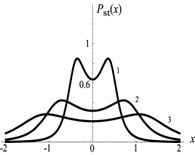
Figure 1: Stationary probability distributions for Lévy flights in symmetric quartic potential $U(x)=\gamma x^{4}/4$ for different values of dimensionless parameter $\beta$: $(1)~{}\beta=0.5$, $(2)~{}\beta=1$, $(3)~{}\beta=1.5$.

The superdiffusion in the form of Lévy flight gives rise to a bimodal stationary probability distribution, when the particle moves in a monostable potential. This bimodal distribution is a peculiarity of Lévy flights. In fact the ordinary diffusion of the Brownian motion is characterized by unimodal SPD. The SPD of superdiffusion has two maxima at the points $x=\pm\beta/\sqrt{2}$, with the value $\left(P_{st}\right)_{max}=4/\left(3\pi\beta\right)$. Since the value of the minimum is $P_{st}\left(0\right)=1/\left(\pi\beta\right)$, the ratio between maximum and minimum value is constant and equal to $4/3$. The variance of the particle coordinate, obtained from Eq. (1) is finite: $\langle X^{2}\rangle_{st}=\beta^{2}$. As a result, the probability distribution becomes more wide with increasing parameter $\beta=\sqrt[3]{D/\gamma}$, that is with decreasing the steepness $\gamma$ of the quartic potential profile, or with increasing the noise intensity $D$.

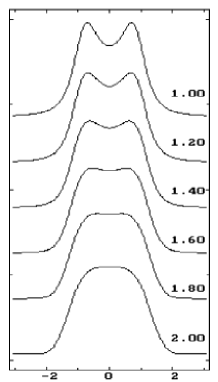
Figure 2: Forms of stationary probability distribution in the symmetric quartic potential for different Lévy indices, from $\alpha=1$ till $\alpha=2$. From Ref. [Chechkin et al., 2002a].

A detailed analysis of the solution of the differential equation (89), for arbitrary Lévy index $\alpha$ and quartic potential $(m=2)$ was performed in Refs. [Chechkin et al., 2002a, 2004]. In Fig. 2 the profiles of SPD (obtained by an inverse Fourier transformation) in symmetric quartic potential are shown for the different Lévy indices from $\alpha=1$, at the top of the figure, up to $\alpha=2$ at the bottom [Chechkin et al., 2002a]. It is seen that the bimodality is most strongly expressed for $\alpha=1$ (Cauchy stable noise source). By increasing the Lévy index, the bimodal profile smoothes out, and, finally, it turns into a unimodal one at $\alpha=2$, recovering the Boltzmann distribution.
Carrying out analogous procedure we obtain the stationary probability distributions for the cases $m=3,4,5$ [Dubkov & Spagnolo, 2007]

$$P_{st}\left(x\right) = \frac{\beta^{5}}{\pi\left(x^{2}+\beta^{2}\right)\left(x^{4}-2\beta^{2}x^{2}\cos\pi/5+\beta^{4}\right)}\,,$$

$$P_{st}\left(x\right) = \frac{\beta^{7}}{\pi\left(x^{4}-2\beta^{2}x^{2}\cos\pi/7+\beta^{4}\right)\left(x^{4}+2\beta^{2}x^{2}\cos 2\pi/7+\beta^{4}\right)}\,,$$ (99)

$$P_{st}\left(x\right) = \frac{\beta^{9}}{\pi\left(x^{2}+\beta^{2}\right)\left(x^{4}-2\beta^{2}x^{2}\cos\pi/9+\beta^{4}\right)\left(x^{4}+2\beta^{2}x^{2}\cos 4\pi/9+\beta^{4}\right)}\,.$$

The plots of distributions (99), for different values of parameter $\beta$, are respectively shown in Figs. 3–5.
It must be emphasized that according to Figs. 3–5, these distributions remain bimodal and have the same tendency with increasing $\beta$, but the ratio between maximum and minimum increases with increasing $m$. From Eqs. (98) and (99) we see that the second moment of the particle coordinate is finite for $m\geq 2$, which confirms the inequality (91). This means that there is a confinement of the particle motion due to the steep potential profile, even if the particle moves according to a superdiffusion in the form of Lévy flights. The presence of two maxima is a peculiarity of the superdiffusion motion. Because of the fast diffusion due to Lévy flights, the particle reaches very quickly regions near the potential walls on the left or on the right with respect to the origin $x=0$. Then the particle diffuses around this position, until a

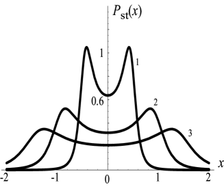
Figure 3: Stationary probability distributions for Lévy flights in symmetric potential $U(x)=\gamma x^{6}/6$ for different values of dimensionless parameter $\beta$: $(1)~{}\beta=0.5$, $(2)~{}\beta=1$, $(3)~{}\beta=1.5$.

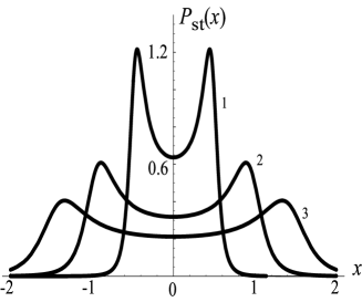
Figure 4: Stationary probability distributions for Lévy flights in symmetric potential $U(x)=\gamma x^{8}/8$ for different values of dimensionless parameter $\beta$: $(1)~{}\beta=0.5$, $(2)~{}\beta=1$, $(3)~{}\beta=1.5$.

new flight moves it in the opposite direction to reach the other potential wall. As a result, the particle spends a large time in some

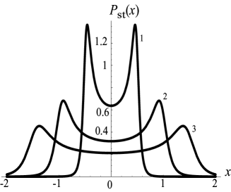
Figure 5: Stationary probability distributions for Lévy flights in symmetric potential $U(x)=\gamma x^{10}/10$ for different values of dimensionless parameter $\beta$: $(1)~{}\beta=0.5$, $(2)~{}\beta=1$, $(3)~{}\beta=1.5$.

symmetric areas with respect to the point $x=0$, differently from the Brownian diffusion in monostable potential profiles. These symmetric areas lie near the maxima of the bimodal SPD. For fixed $D$ and $m$, these maxima are closer or far away the point $x=0$ depending on the greater or smaller steepness $\gamma$ of the potential profile. This corresponds to a greater or smaller confinement of the particle motion. Of course, such confinement is more pronounced for greater $m$, that is for steeper potential profiles.
On the basis of Eqs. (97)–(99) and the known behavior of density tails (90), we can write the general expressions for stationary probability distribution in the case of potential $U\left(x\right)=\gamma x^{2m}/\left(2m\right)$ with odd $m=2n+1$ [Dubkov & Spagnolo, 2007]

$$P_{st}\left(x\right)=\frac{\beta^{4n+1}}{\pi\left(x^{2}+\beta^{2}\right)}\prod\limits_{l=0}^{n-1}\frac{1}{x^{4}-2\beta^{2}x^{2}\cos\left[\pi\left(4l+1\right)/\left(4n+1\right)\right]+\beta^{4}}\,,$$ (100)

and even $m=2n$

$$P_{st}\left(x\right)=\frac{\beta^{4n-1}}{\pi}\prod\limits_{l=0}^{n-1}\frac{1}{x^{4}-2\beta^{2}x^{2}\cos\left[\pi\left(4l+1\right)/\left(4n-1\right)\right]+\beta^{4}}\,.$$ (101)

The strong proof of non-unimodality of the SPD for symmetric monostable potential $U\left(x\right)=\left|x\right|^{c}/c$ in the case $c>2$ was given in Ref. [Chechkin et al., 2004]. Indeed, from Eq. (83) we have for SPD

$$\frac{d}{dx}\left[\left|x\right|^{c-1}\mathrm{sgn}~{}x\cdot P_{st}\right]+D\frac{d^{\alpha}P_{st}}{d\left|x\right|^{\alpha}}=0.$$ (102)

As a result, from Eqs. (102) and (60) at the point $x=0$ we obtain

$$\left.\frac{d^{\alpha}P_{st}}{d\left|x\right|^{\alpha}}\right|_{x=0}=\int_{-\infty}^{+\infty}\frac{P_{st}\left(-z\right)-P_{st}\left(0\right)}{\left|z\right|^{\alpha+1}}=0.$$ (103)

Because of the symmetry of the SPD $P_{st}\left(x\right)$, Eq. (103) gives

$$\int_{0}^{\infty}\frac{P_{st}\left(z\right)-P_{st}\left(0\right)}{z^{\alpha+1}}=0.$$ (104)

For unimodal probability distribution with the maximum at the origin, the integral in the left side of Eq. (104) should be negative, which contradicts Eq. (104).
The estimation of bifurcation time for transition from unimodal initial distribution to bimodal stationary one for the quartic potential $(c=4)$ was done in Refs. [Chechkin et al., 2004, 2006]. The dependence of this bufurcation time $t_{12}$ from Lévy index $\alpha$ is plotted in Fig. 6.

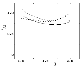
Figure 6: Bifurcation time $t_{12}$ versus Lévy index $\alpha$ for quartic potential. Black dots: bifurcation time deduced from the numerical solution of the fractional Fokker -Planck equation. Dashed and solid lines: two subsequent approximations. From Refs. [Chechkin et al., 2004, 2006].

Also authors proved an existence of a transient trimodal state between initial unimodal and final bimodal ones. This evolution, shown in Fig. 7, can be only observed for monostable potential with $c>4$ and for fixed values of the Lévy index $\alpha$.

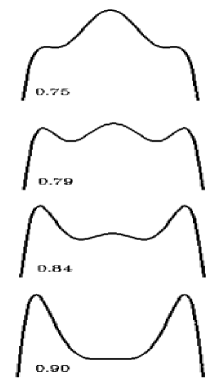
Figure 7: The evolution of the probability distribution for $\alpha=1.2$ and $c=5.5$ from unimodal through trimodal to bimodal. From Refs. [Chechkin et al., 2004, 2006].

The corresponding bifurcation times of transitions $t_{13}$ (unimodal $\rightarrow$ trimodal) and $t_{32}$ (trimodal $\rightarrow$ bimodal) versus Lévy index $\alpha$, with potential exponent $c=5.5$, are plotted in Fig. 8.

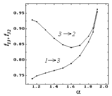
Figure 8: Bifurcation times $t_{13}$ and $t_{32}$ versus Lévy index $\alpha$ for the power potential with the exponent $c=5.5$. From Ref. [Chechkin et al., 2004].

X Barrier crossing

The problem of escape from metastable states investigated by Kramers [Kramers, 1940] is ubiquitous in almost all scientific areas [Hänggi et al., 1990; Spagnolo et al., 2007]. Since many stochastic processes do not obey the Central Limit Theorem, the corresponding Kramers escape behavior will differ. An interesting example is given by the $\alpha$-stable noise-induced barrier crossing in long paleoclimatic time series [Ditlevsen, 1999a]. Another new application is the escape from traps in optical or plasma systems [Fajans & Schmidt, 2004].
The main tools to investigate the barrier crossing problem for Lévy flights are the first passage times, crossing times, arrival time and residence times. We should emphasize that the problem of mean first passage time (MFPT) meets with some difficulties because free Lévy flights represent a special class of discontinuous Markovian processes with infinite mean squared displacement. First of all, the fractional Fokker-Planck equation (83) is integro-differential, and the conditions at absorbing and reflecting boundaries differ from the usual conditions for ordinary diffusion. Superdiffusion motion is characterized by the presence of jumps, and, as a result, a particle can reach instantaneously the boundary from arbitrary position. One can mention some erroneous results for Lévy flights obtained in Ref. [Gitterman, 2000], because author used the traditional conditions at two absorbing boundaries (see the related correspondence [Yuste & Lindenberg, 2004; Gitterman, 2004]). The numerical results for the first passage time of free Lévy flights confined in a finite interval were presented in Ref. [Dybiec et al., 2006]. The complexity of the first passage time statistics (mean first passage time, cumulative first passage time distribution) was elucidated together with a discussion of the proper setup of corresponding boundary conditions, that correctly yield the statistics of first passages for these non-Gaussian noises. In particular, it has been demonstrated by numerical studies that the use of the local boundary condition of vanishing probability flux in the case of reflection, and vanishing probability in the case of absorbtion, valid for normal Brownian motion, no longer apply for Lévy flights. This in turn requires the use of nonlocal boundary conditions. Dybiec with co-authors found a nonmonotonic behavior of the MFPT for two absorbing boundaries, with the maximum being assumed for $\alpha=1$ (see Fig. 9), in contrast with a monotonic increase for reflecting and absorbing boundaries.

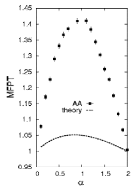
Figure 9: Mean first passage time versus Lévy index $\alpha$ of confined motion between two absorbing boundaries driven by stable symmetric Lévy white noise. From Ref. [Dybiec et al., 2006].

According to the Kramers law, the probability distribution of the escape time from a potential well with the barrier of height $U_{0}$, has the exponential form

$$p\left(t\right)=\frac{1}{T_{c}}\exp\left\{-\frac{t}{T_{c}}\right\}$$ (105)

with mean crossing time

$$T_{c}=C\exp\left\{\frac{U_{0}}{D}\right\},$$ (106)

where $C$ is some positive prefactor and $D$ is the noise intensity. The problem how the stable nature of Lévy flight processes generalizes the barrier crossing behavior of the classical Kramers problem was investigated, both numerically and analytically, in Ref. [Chechkin et al., 2003b, 2005, 2006, 2007]. Authors considered Lévy flights in a bistable potential $U\left(x\right)$ by numerical solution of Eq. (85). It was shown that although the survival probability decays again exponentially as in Eq. (105), the mean escape time $T_{c}$ has a power-law dependence on the noise intensity $D$

$$T_{c}\simeq\frac{C(\alpha)}{D^{\mu(\alpha)}}\,,$$ (107)

where the prefactor $C$ and the exponent $\mu$ depend on the Lévy index $\alpha$. Using the Fourier transform, i.e. Eq. (87), the mean escape rate was found for large values of $1/D$ in the case of Cauchy stable noise $\left(\alpha=1\right)$ in the framework of the constant flux approximation across the barrier. The probability law and the mean value of escape time from a potential well for all values of the stability index $\alpha\in(0,2)$, in the limit of small Lévy driving noise, were also determined in the paper [Imkeller & Pavlyukevich, 2006] by purely probabilistic methods. Escape times had the same exponential distribution (105), and the mean value depends on the noise intensity $D$ in accordance with Eq. (107) with $\mu(\alpha)=1$ and pre-factor $C$ depending on $\alpha$ and the distance between the local extrema of the potential.
The barrier crossing of a particle driven by symmetric Lévy noise of index $\alpha$ and intensity $D$ for three different generic types of potentials was numerically investigated in Ref. [Chechkin et al., 2007]. Specifically: (i) a bistable potential, (ii) a metastable potential, and (iii) a truncated harmonic potential, were considered. For the low noise intensity regime, the result of Eq. (107) was recovered. As it was shown, the exponent $\mu(\alpha)$ remains approximately constant, $\mu\approx 1$ for $0<\alpha<2$; at $\alpha=2$ the power-law form of $T_{c}$ changes into the exponential dependence (106). It exhibits a divergence-like behavior as $\alpha$ approaches $2$. In this regime a monotonous increase of the escape time $T_{c}$ with increasing $\alpha$ (keeping the noise intensity $D$ constant) was observed. For low noise intensities the escape times correspond to barrier crossing by multiple Lévy steps. For high noise intensities, the escape time curves collapse for all values of $\alpha$. At intermediate noise intensities, the escape time exhibits non-monotonic dependence on the index $\alpha$ as in Fig. 9, while still retains the exponential form of the escape time density.
The first arrival time is an appropriate parameter to analyze the barrier crossing problem for Lévy flights. If we insert in fractional Fokker-Planck equation (83) a $\delta$-sink of strength $q\left(t\right)$ in the origin, we obtain the following equation for the non-normalized probability density function $P\left(x,t\right)$

$$\frac{\partial P}{\partial t}=\frac{\partial}{\partial x}\left[U^{\prime}\left(x\right)P\right]+D\frac{\partial^{\alpha}P}{\partial\left|x\right|^{\alpha}}-q\left(t\right)\delta\left(x\right),$$ (108)

from which by integration over all space we may define the quantity

$$q\left(t\right)=-\frac{d}{dt}\int_{-\infty}^{+\infty}P\left(x,t\right)dx,$$ (109)

which is the negative time derivative of the survival probability. According to definition (109), $q\left(t\right)$ represents the probability density function of the first arrival time: once a random walker arrives at the sink it is annihilated. As it was shown in the paper [Chechkin et al., 2003b] for free Lévy flights $\left(U\left(x\right)=0\right)$, the first arrival time distribution has a heavy tail

$$q\left(t\right)\sim t^{1/\alpha-2}$$ (110)

with exponent depending on Lévy index $\alpha$ $\left(1<\alpha<2\right)$ and differing from universal Sparre Andersen result [Sparre Andersen, 1953, 1954] for the probability density function of first passage time for arbitrary Markovian process

$$p\left(t\right)\sim t^{-3/2}.$$ (111)

In the Gaussian case $\left(\alpha=2\right)$, the quantity (110) is equivalent to the first passage time probability density (111). From a random walk perspective, this is due to the fact that individual steps are of the same increment, and the jump length statistics therefore ensures that the walker cannot hop across the sink in a long jump without actually hitting the sink and being absorbed. This behavior becomes drastically different for Lévy jump length statistics: there, the particle can easily cross the sink in a long jump. Thus, before eventually being absorbed, it can pass by the sink location numerous times, and therefore the statistics of the first arrival will be different from that of the first passage. The result (111) for Lévy flights was also confirmed numerically in the paper [Koren et al., 2007].
At last, the nonlinear relaxation time technique is also suitable for investigations of Lévy flights temporal characteristics. According to definition, the mean residence time in the interval $\left(L_{1},L_{2}\right)$ reads

$$T\left(x_{0}\right)=\int_{0}^{\infty}dt\int_{L_{1}}^{L_{2}}P\left(\left.x,t\right|x_{0},0\right)dx,$$ (112)

where $x_{0}$ is the initial position of all particles $\left(x_{0}\in\left(L_{1},L_{2}\right)\right)$ and $P\left(\left.x,t\right|x_{0},0\right)$ is the probability density of transitions. We do not need to think about the boundary conditions in this case because we are concerned with the overall time spent by the particle in the fixed interval. Changing the order of integration in Eq. (112) we obtain

$$T\left(x_{0}\right)=\int_{L_{1}}^{L_{2}}Y\left(x,x_{0},0\right)dx,$$ (113)

where $Y\left(x,x_{0},s\right)$ is the Laplace transform of the transient probability density $P\left(\left.x,t\right|x_{0},0\right)$

$$Y\left(x,x_{0},s\right)=\int_{0}^{\infty}P\left(\left.x,t\right|x_{0},0\right)e^{-st}dt.$$ (114)

Making the Laplace transform in the fractional Fokker-Planck equation (83) and taking into account the initial condition $P\left(\left.x,0\right|x_{0},0\right)=\delta\left(x-x_{0}\right)$, we get

$$\frac{d}{dx}\left[U^{\prime}\left(x\right)Y\right]+D\frac{d^{\alpha}Y}{d\left|x\right|^{\alpha}}-sY=-\delta\left(x-x_{0}\right).$$ (115)

If we put $s=0$ in Eq. (115) and make the Fourier transform we obtain

$$U^{\prime}\left(-i\frac{d}{dk}\right)\widetilde{Y}-iD\left|k\right|^{\alpha-1}\mathrm{sgn}\left(k\right)\widetilde{Y}=\frac{e^{ikx_{0}}}{ik},$$ (116)

where

$$\widetilde{Y}\left(k,x_{0}\right)=\int_{-\infty}^{+\infty}Y\left(x,x_{0},0\right)e^{+ikx}dx.$$ (117)

After solving Eq. (116) we can calculate the mean residence time as (see Eqs. (113) and (117))

$$T\left(x_{0}\right)=\frac{1}{2\pi i}\int_{-\infty}^{+\infty}\frac{e^{-ikL_{1}}-e^{-ikL_{2}}}{k}\widetilde{Y}\left(k,x_{0}\right)dk.$$ (118)

Equations (116) and (118) are useful tools to analyze the temporal characteristics of Lévy flights in different potential profiles $U\left(x\right)$.

XI Conclusions

In this tutorial paper, after some short historical notes on normal diffusion and superdiffusion, we introduce the Lévy flights as self-similar Lévy processes. After the definition of the strictly stable random variables, the subfamily of the Lévy motion is introduced with the fractional differential equation for Lévy flight superdiffusion. We used then functional analysis approach to derive the fractional Fokker-Planck equation directly from Langevin equation with symmetric $\alpha$-stable Lévy noise. This approach allows to describe anomalous diffusion in the form of Lévy flights. We obtained the general formula for stationary probability distribution of superdiffusion in symmetric smooth monostable potential for Cauchy driving noise. All distributions have bimodal shape and become more narrow with increasing steepness of the potential or with decreasing noise intensity. We found that the variance of the particle coordinate is finite for quartic potential profile and for steeper potential profiles, that is a confinement of the particle in a superdiffusion motion in the form of Lévy flights. As a result, we can evaluate the power spectral density of a stationary motion. We have also discussed recently obtained analytical and numerical results for time characteristics of Lévy flights. Special attention was given for some difficulties with formulation of the correct boundary conditions for mean first passage time problem. As it was shown, the arrival and residence times are more appropriate characteristics for investigations of Lévy flights in different potential profiles.

Acknowledgments

This work has been supported by MIUR, CNISM, and by Russian Foundation for Basic Research (projects 07-01-00517 and 08-02-01259).

References

- (1) Albano, E. V. [1991] ”Diffusion and annihilation reactions of Lévy flights with bounded long-range hoppings,” J. Phys. A: Math. Gen. 24, 3351–3358.
- (2) Albano, E. V. [1996] ”Branching annihilating Lévy flights: Irreversible phase transitions with long-range exchanges,” Europhys. Lett. 34, 97–102.
- (3) Annunziato, M., Grigolini, P. & West, B. J. [2001] ”Canonical and noncanonical equilibriu distribution,” Phys. Rev. E 64, 011107-1–011107-13.
- (4) Bachelier, L. [1900] ”Théorie de la spéculation,” (Thèse) Annales Scientifiques de l’École Normale Supérieure 3, 21–86.
- (5) Bao, J-D., Wang, H-Y., Jia, Y. & Zhuo, Y-Zh. [2005] ”Cancellation phenomenon of barrier escape driven by a non-Gaussian noise,” Phys. Rev. E 72, 051105-1–051015-4.
- (6) Bardou, F., Bouchaud, J. P., Emile, O., Aspect, A. & Cohen-Tannoudji, C. [1994] ”Subrecoil laser cooling and Lévy flights,” Phys. Rev. Lett. 72, 203–206.
- (7) Bardou, F., Bouchaud, J. P., Aspect, A. & Cohen–Tannoudji, C. [2002] Lévy Statistics and Laser Cooling (Cambridge University Press, Cambridge)
- (8) Barkai, E. [2004] ”Stable Equilibrium Based on Lévy Statistics: A Linear Boltzmann Equation Approach,” J. Stat. Phys. 115, 1537–1565.
- (9) Bergersen, B. & Rácz, Z. [1991] ”Dynamical Generation of Long-Range Interactions: Random Lévy Flights in the Kinetic Ising and Spherical Models,” Phys. Rev. Lett. 67, 3047–3050.
- (10) Bertoin, J. [1996] Lévy processes (Cambridge University Press, Cambridge).
- (11) Boldyrev, S. & Gwinn, C. [2003] ”Scintillations and Lévy flights through the interstellar medium,” Astrophys. J. 584, 791–796.
- (12) Bologna, M., Grigolini, P. & Riccardi, J. [1999] ”Lévy diffusion as an effect of sporadic randomness,” Phys. Rev. E 60, 6435–6442.
- (13) Bouchaud, J.-B. & Sornette, D. [1994] ”The Black-Scholes option pricing problem in mathematical finance: Generalization and extensions for a large class of stochastic processes,” J. Phys. I (Paris) 4, 863–881.
- (14) Brockmann, D. & Sokolov, I. M. [2002] ”Lévy flights in external force fields: from models to equations,” Chem. Phys. 284, 409–421.
- (15) Brown, R. [1828] ”A brief account of microscopical observations made in the months of June, July, and August, 1827, on the particles contained in the pollen of plants; and on the general existence of active molecules in organic and inorganic bodies,” Philos. Mag. 4, 161–173.
- (16) Buldyrev, S. V., Havlin, S., Kazakov, A. Ya., da Luz, M. G. E., Raposo, E. P., Stanley, H. E. & Viswanathan, G. M. [2001] ”Average time spent by Lévy flights and walks on an interval with absorbing boundaries,” Phys. Rev. E 64, 041108-1–041108-11.
- (17) Cabrera, J. L. & Milton, J. G. [2004] ”Human stick balancing: Tuning Lévy flights to improve balance control,” Chaos 14, 691–698.
- (18) Cáceres, M. O. [1999] ”Lévy noise, Lévy flights, Lévy fluctuations,” J. Phys. A: Math. Gen. 32, 6009 -6019.
- (19) Carati, A., Galgani, L. & Pozzi, B. [2003] ”Lévy Flights in the Landau-Teller Model of Molecular Collisions,” Phys. Rev. Lett. 90, 010601-1–010601-4.
- (20) Chandrasekhar, S. [1943] ”Stochastic Problems in Physics and Astronomy,” Rev. Mod. Phys. 15, 1–89.
- (21) Chaves, A. S. [1998] ”A fractional diffusion equation to describe Lévy flights,” Phys. Lett. A 239, 13–16.
- (22) Chechkin, A. V. & Gonchar, V. Yu. [2000] ”A model for persistent Lévy motion,” Physica A 277, 312–326.
- (23) Chechkin, A. V., Gonchar, V., Klafter, J., Metzler, R. & Tanatarov, L. [2002a] ”Stationary states of non-linear oscillators driven by Lévy noise,” Chem. Phys. 284, 233–251.
- (24) Chechkin, A. V., Gonchar, V. Y. & Szydlowsky, M. [2002b] ”Fractional kinetics for relaxation and superdiffusion in a magnetic field,” Phys. Plasma 9, 78–88.
- (25) Chechkin, A. V., Gorenflo, R. & Sokolov, I. M. [2002c] ”Retarding sub– and accelerating super–diffusion governed by distributed order fractional diffusion equations,” Phys. Rev. E 66, 046129-1–046129-7.
- (26) Chechkin, A. V., Klafter, J., Gonchar, V. Yu., Metzler, R. & Tanatarov, L. V. [2003a] ”Bifurcation, bimodality, and finite variance in confined Lévy flights,” Phys. Rev. E 67, 010102-1–010102-4.
- (27) Chechkin, A. V., Metzler, R., Gonchar, V. Yu., Klafter, J. & Tanatarov, L. V. [2003b] ”First passage and arrival time densities for Lévy flights and the failure of the method of images,” J. Phys. A: Math. Gen. 36, L537–L544.
- (28) Chechkin, A. V., Gonchar, V. Yu., Klafter, J., Metzler, R. & Tanatarov, L. V. [2004] ”Lévy flights in a steep potential well,” J. Stat. Phys. 115, 1505–1535.
- (29) Chechkin, A. V., Gonchar, V. Yu., Klafter, J. & Metzler, R. [2005] ”Barrier crossing of a Lévy flight,” Europhys. Lett. 72, 348–354.
- (30) Chechkin, A. V., Gonchar, V. Yu., Klafter, J. & Metzler, R. [2006] ”Fundamentals of L evy flight processes,” Adv. Chem. Phys. 133, 439–496.
- (31) Chechkin, A. V., Sliusarenko, O. Yu., Metzler, R. & Klafter, J. [2007] ”Barrier crossing driven by Lévy noise: Universality and the role of noise intensity,” Phys. Rev. E 75, 041101-1–041101-11.
- (32) Chowdhury, D. & Stauffer, D. [1999] ”A generalized spin model of financial markets,” Eur. Phys. J. B 8, 477–482.
- (33) Cole, B. J. [1995] ”Fractal time in animal behaviour: the movement activity of Drosophila,” Anim. Behav. 50, 1317–1324.
- (34) de Finetti, B. [1929] ”Sulle funzioni ad incremento aleatorio,” Rendiconti della R. Accademia Nazionale dei Lincei (Ser VI) 10, 325–329.
- (35) de Finetti, B. [1975] Theory of probability, Vol. 1,2 (Wiley, New York).
- (36) del-Castillo-Negrete, D., Carreras, B. A. & LynchCole V. E. [2003] ”Front Dynamics in Reaction-Diffusion Systems with Lévy Flights: A Fractional Diffusion Approach,” Phys. Rev. Lett. 91, 018302-1–018302-4.
- (37) Desbois, J. [1992] ”Asymptotic winding angle distributions for two-dimensional Lévy flights,” J. Phys. A: Math. Gen. 25, L195–Ll99.
- (38) Ditlevsen, P. D. [1999a] ”Observation of alpha–stable noise and a bistable climate potential in an ice–core record,” Geophys. Res. Lett. 26, 1441–1444.
- (39) Ditlevsen, P. D. [1999b] ”Anomalous jumping in a double–well potential,” Phys. Rev. E 60, 172–179.
- (40) Doob, J. L. [1953] Stochastic Processes (Wiley, New York).
- (41) Dubkov, A. & Spagnolo, B. [2005] ”Generalized Wiener process and Kolmogorov’s equation for diffusion induced by non–Gaussian noise source,” Fluct. Noise Lett. 5, L267–L274.
- (42) Dubkov, A. & Spagnolo, B. [2007] ”Langevin Approach to Lévy Flights in Fixed Potentials: Exact Results for Stationary Probability Distributions,” Acta Phys. Pol. B 38, 1745–1758.
- (43) Dybiec, B. & Gudowska-Nowak, E. [2004] ”Resonant activation in the presence of nonequilibrated baths,” Phys. Rev. E 69, 016105-1–016105-7.
- (44) Dybiec, B., Gudowska-Nowak, E. & Hänggi, P. [2006] ”Lévy–Brownian motion on finite intervals: Mean first passage time analysis,” Phys. Rev. E 73, 046104-1–046104-9.
- (45) Dybiec, B., Gudowska-Nowak, E. & Hänggi, P. [2007] ”Escape driven by alpha–stable white noises,” Phys. Rev. E 75, 021109-1–021109-8.
- (46) Edwards, A. M., Phillips, R. A., Watkins, N. W., Freeman, M. P., Murphy, E. J., Afanasyev, V., Buldyrev, S. V., da Luz, M. G. E., Raposo, E. P., Stanley, H. E. & Viswanathan, G. M. [2007] ”Revisiting Lévy flight search patterns of wandering albatrosses, bumblebees and deer,” Nature 449, 1044–1048.
- (47) Einstein, A. [1905] ”Uber die von der molekularkinetischen Theorie der Warme geforderte Bewegung von in ruhenden Flussigkeiten suspendierten Teilchen,” (Concerning the motion, as required by the molecular-kinetic theory of heat, of particles suspended in liquid at rest), Ann. Phys. (Leipzig) 17, 549–556.
- (48) Eliazar, I. & Klafter, J. [2003] ”Lévy–Driven Langevin Systems: Targeted Stochasticity,” J. Stat. Phys. 111, 739–768.
- (49) Fajans, J. & Schmidt, A. [2004] ”Malmberg -Penning and Minimum-B trap compatibility: the advantages of higher-order multipole traps,” Nucl. Instrum. & Methods in Phys. Res. A 521, 318–325.
- (50) Feller, W. [1971] An Introduction to Probability Theory and its Applications, Vol. 2 (John Wiley & Sons, Inc., New York).
- (51) Ferraro, M. & Zaninetti, L. [2006] ”Mean number of visits to sites in Lévy flights,” Phys. Rev. E 73, 057102-1–057102-4.
- (52) Fogedby, H. C. [1994a] ”Lévy Flights in Random Environments,” Phys. Rev. Lett. 73, 2517–2520.
- (53) Fogedby, H. C. [1994b] ”Langevin equations for continuous time Lévy flights,” Phys. Rev. E 50, 1657–1660.
- (54) Fogedby, H. C. [1998] ”Lévy flights in quenched random force fields,” Phys. Rev. E 58, 1690–1712.
- (55) Fokker, A. D. [1914] ”Die mittlere Energie rotierender elektrischer Dipole im Strahlungsfeld,” (The average energy of a rotating electric dipoles in a radiation field.) Ann. Phys. (Leipzig) 43, 810–820.
- (56) Furutsu, K. [1963] ”On the statistical theory of electromagnetic waves in a fluctuating medium,” J. Res. Natl. Bur. Stand. D 67, 303–323.
- (57) Garbaczewski, P. & Olkiewicz, R. [2000] ”Ornstein–Uhlenbeck–Cauchy Process,” J. Math. Phys. 41, 6843–6860.
- (58) Garoni, T. M. & Frankel, N. E. [2002] ”Lévy flights: Exact results and asymptotics beyond all orders,” J. Math. Phys. 43 2670–2689.
- (59) Gitterman, M. [2000] ”Mean first passage time for anomalous diffusion,” Phys. Rev. E 62, 6065–6070.
- (60) Gitterman, M. [2004] ”Reply to ”Comment on ’Mean first passage time for anomalous diffusion’”,” Phys. Rev. E 69, 033102-1–033102-2.
- (61) Gnedenko, B. V. & Kolmogorov, A. N. [1954] Limit Distributions for Sums of Independent Random Variables (Addison–Wesley, Cambridge) [English translation from the Russian edition, GITTL, Moscow (1949)].
- (62) Gorenflo, R. & Mainardi, F. [2005] ”Simply and multiply scaled diffusion limits for continuous time random walks,” J. Phys., Conference series (JPCS) 7 1–16.
- (63) Govorun, E. N., Ivanov, V. A., Khokhlov, A. R., Khalatur, P. G., Borovinsky, A. L. & Grosberg, A. Yu. [2001] ”Primary sequences of proteinlike copolymers: Lévy–flight -type long-range correlations,” Phys. Rev. E 64, 040903-1–040903-4(R).
- (64) Grassberger, P. [1985] ”Critical exponents of self-avoiding Lévy flights,” J. Phys. A: Math. Gen. 18, L463–L467.
- (65) Grigolini, P., Rocco, A. & West, B. J. [1999] ”Fractional calculus as a macroscopic manifestation of randomness,” Phys. Rev. E 59, 2603–2613.
- (66) Hänggi, P. [1978] ”Correlation Functions and Master Equations of Generalized (Non-Markovian) Langevin Equations,” Z. Physik B 31, 407–416.
- (67) Hänggi, P., Talkner, P. & Borkovec, M. [1990] ”Reaction-rate theory: fifty years after Kramers,” Rev. Mod. Phys. 62, 251–341.
- (68) Imkeller, P. & Pavlyukevich, I. [2006] ”Lévy flights: transitions and meta–stability,” J. Phys. A: Math. Gen. 39, L237–L246.
- (69) Imkeller, P., Pavlyukevich, I. & Wetzel, T. [2007] ”First exit times for Lévy-driven diffusions with exponentially light jumps,” arXiv:0711.0982v1 [math.PR], 6 Nov 2007, pp 1–30.
- (70) Itô, K. [1944] ”Stochastic Integral,” Proc. Imp. Acad. 20, 519–524.
- (71) Itô, K. [1946] ”On a stochastic differential equation,” Proc. Japan Acad. 22, 32–35.
- (72) Itô, K. & McKean, H. [1965] Diffusion Processes and Their Sample Paths (Springer-Verlag, Berlin).
- (73) Janssen, H. K., Oerding, K., van Wijland, F. & Hilhorst, H. J. [1999] ”Lévy-flight spreading of epidemic processes leading to percolating clusters,” Eur. Phys. J. B 7, 137–145.
- (74) Jespersen, S., Metzler, R. & Fogedby, H. C. [1999] ”Lévy flights in external force fields: Langevin and fractional Fokker–Planck equations and their solutions,” Phys. Rev. E 59, 2736–2745.
- (75) Kaç, M. [1957] Probability and Related Topics in Physical Science (Lectures in Applied Mathematics, Vol. 1a, American Mathematical Society).
- (76) Kamińska, A. & Srokowski, T. [2004] ”Simple jumping process with memory: Transport equation and diffusion,” Phys. Rev. E 69, 062103-1–062103-4.
- (77) Katori, H., Schlipf, S. & Walther, H. [1997] ”Anomalous Dynamics of a Single Ion in an Optical Lattice,” Phys. Rev. Lett. 79, 2221–2224.
- (78) Khintchine, A. & Lévy, P. [1936] ”Sur les lois stables,” Comptes Rendus 202, 374–376.
- (79) Khintchine, A. Ya. [1938] Limit distributions for the sum of independent random variables (O.N.T.I., Moscow) [in Russian].
- (80) Klyatskin, V. I. [1974] ”Statistical theory of light reflection in randomly inhomogeneous medium,” Sov. Phys. JETP 38, 27–34.
- (81) Kolmogorov, A. N. [1941] ”The local structure of turbulence in an incompressible fluid for very large Reynolds numbers,” C.R. Acad. Sci. USSR 30, 301–305.
- (82) Koren, T., Chechkin, A. V. & Klafter, J. [2007] ”On the first passage time and leapover properties of Lévy motions,” Physica A 379, 10–22.
- (83) Kramers, H. A. [1940] ”Brownian motion in a field of force and the diffusion model of chemical reactions,” Physica 7, 284–304.
- (84) Kusnezov, D., Bulgac, A. & Dang, G. D. [1999] ”Quantum Lévy Processes and Fractional Kinetics,” Phys. Rev. Lett. 82 1136–1139.
- (85) Kutner, R. & Maass, P. [1998] ”Lévy flights with quenched noise amplitudes,” J. Phys. A: Math. Gen. 31, 2603 -2609.
- (86) Langevin, P. [1908] ”Sur la théorie du mouvement brownien,” Comptes Rendus 146, 530–533.
- (87) Lenzi, E. K., Mendes, R. S., Fa, K. S., Malacarne, L. C. & da Silva, L. R. [2003] ”Anomalous diffusion: Fractional Fokker–Planck equation and its solutions,” J. Math. Phys. 44 2179–2185.
- (88) Levandowsky, M., White, B. S. & Schuster, F. L. [1997] ”Random movements of soil amoebas,” Acta Protozool. 36, 237–248.
- (89) Lévy, P. [1925] Calcul des Probabilités (Gauthier–Villars, Paris).
- (90) Lévy, P. [1937] Theory de l’addition des variables Aléatoires (Gauthier–Villars, Paris).
- (91) Lévy, P. [1965] Processus stochastiques et mouvement brownien (Gauthier–Villars, Paris).
- (92) Loève, M. [1963] Probability Theory, 3rd ed. (Van Nostrand, Princeton)
- (93) Lomholt, M. A., Ambjörnsson, T. & Metzler, R. [2005] ”Optimal Target Search on a Fast–Folding Polymer Chain with Volume Exchange,” Phys. Rev. Lett. 95, 260603-1–260603-4.
- (94) Lynch, V. E., Carreras, B. A., del-Castillo-Negrete, D., Ferreira-Mejias, K. M. & Hicks H. R. [2003] ”Numerical methods for the solution of partial differential equations of fractional order,” J. Comput. Phys. 192, 406 -421.
- (95) Mainardi, F., Luchko, Yu. & Pagnini, G. [2001] ”The fundamental solution of the space–time fractional diffusion equation,” Fractional Calculus and Applied Analysis 4, 153–192.
- (96) Mainardi, F. & Rogosin, S. [2006] ”The origin of infinitely divisible distributions: from de Finetti s problem to Lévy–Khintchine formula,” Mathematical Methods in Economics and Finance 1, 37–55.
- (97) Mandelbrot, B. B. [1963] ”The Variation of Certain Speculative Prices,” J. Bus. 36, 394–419.
- (98) Mandelbrot, B. B. [1997] Fractals and Scaling in Finance (Springer, New York).
- (99) Mantegna, R. N. [1991] ”Lévy walks and enhanced diffusion in Milan stock exchange,” Physica A 179, 232–242.
- (100) Mantegna, R. N. & Stanley, H. E. [1996] ”Turbulence and financial markets,” Nature 383, 587–588.
- (101) Mantegna, R. N. & Stanley, H. E. [1998] ”Modeling of financial data: Comparison of the truncated Lévy flight and the ARCH(1) and GARCH(1,1) processes,” Physica A 254, 77–84.
- (102) Metzler, R. & Klafter, J. [2000] ”The random walk’s guide to anomalous diffusion: a fractional dynamics approach,” Phys. Rep. 339, 1–77.
- (103) Metzler, R. & Nonnenmacherc T. F. [2002] ”Space- and time-fractional diffusion and wave equations, fractional Fokker Planck equations, and physical motivation,” Chemical Physics 284, 67 -90.
- (104) Metzler, R. & Klafter, J. [2004] ”The restaurant at the end of the random walk: recent developments in the description of anomalous transport by fractional dynamics,” J. Phys. A: Math. Gen. 37, R161 -R208.
- (105) Metzler, R., Chechkin, A. V. & Klafter, J. [2007] ”Lévy Statistics and Anomalous Transport: Lévy flights and Subdiffusions,” arXiv:0706.3553v1 [cond-mat.stat-mech], 25 Jun 2007, pp 1–36.
- (106) Monin, A. S. [1955] ”Equation of turbulent diffusion,” Dokl. Akad. Nauk SSSR 105, 256–259.
- (107) Nikias, C. L. & Shao, M. [1995] Signal Processing with Alpha-Stable Distributions and Applications (John Wiley & Sons, N.Y.)
- (108) Novikov, E. A. [1965] ”Functionals and the random–force method in turbulence theory,” Sov. Phys. JETP 20, 1290–1294.
- (109) Obukhov, A. M. [1941] ”On the distribution of energy in the spectrum of a turbulent flow,” Dokl. Akad. Nauk SSSR 32, 22–24.
- (110) Ott, A., Bouchaud, J. P., Langevin, D. & Urbach, W. [1990] ”Anomalous Diffusion in ”Living Polymers”: A Genuine Lévy Flight?,” Phys. Rev. Lett. 65 2201–2204.
- (111) Painter, S. [1996] ”Evidence of non–Gaussian scaling behaviour in heterogeneous sedimentary formations,” Water Resources Research 32, 1183–1195.
- (112) Pavlyukevich I. [2007] ”Cooling down Lévy flights,” J. Phys. A: Math. Theor. 40, 12299–12313.
- (113) Perrin, J. [1908] ”L’agitation moléculaire et le mouvement brownien,” Comptes Rendus 146, 967–970.
- (114) Planck, M. [1917] ”An essay on statistical dynamics and its amplification in the quantum theory,” Sitz. Ber. Preuss. Akad. Wiss. 325, 324–341.
- (115) Posadas, A., Morales, J., Vidal, F., Sotolongo-Costa, O. & Antoranz, J. C. [2002] ”Continuous time random walks and south Spain seismic series,” J. Seismol. 6, 61–67.
- (116) Rangarajan, G. & Ding, M. [2000a] ”Anomalous diffusion and the first passage time problem,” Phys. Rev. E 62, 120–133.
- (117) Rangarajan, G. & Ding, M. [2000b] ”First passage time distribution for anomalous diffusion,” Phys. Lett. A 273, 322–330.
- (118) Reible, D. & Mohanty, S. [2002] ”A Lévy flight-random walk model for bioturbation,” Envir. Toxicol. Chem. 21, 875 -881.
- (119) Reichel, J., Bardou, F., Ben Dahan, M., Peik, E., Rand, S., Salomon, C. & Cohen–Tannoudji, C. [1995] ”Raman Cooling of Cesium below 3 nK: New Approach Inspired by Lévy Flight Statistics,” Phys. Rev. Lett. 75, 4575–4578.
- (120) Rhodes, T. & Turvey, M. T. [2007] ”Human memory retrieval as Lévy foraging,” Physica A 385, 255 260.
- (121) Richardson, L. [1926] ”Atmospheric diffusion shown on a distance neighbour graph,” Proc. Roy. Soc. A 110, 709–737.
- (122) Saichev, A. I. & Zaslavsky, G. M. [1997] ”Fractional kinetic equations: solutions and applications,” Chaos 7, 753–764.
- (123) Sato, K. I. [1999] Lévy Processes and Infinitely Divisible Distributions (Cambridge University Press, Cambridge).
- (124) Scafetta, N., Latora, V. & Grigolini, P. [2002] ”Lévy scaling: The diffusion entropy analysis applied to DNA sequences,” Phys. Rev. E 66, 031906-1–031906-15.
- (125) Schaufler, S., Schleich, W. P. & Yakovlev, V. P. [1997] ”Scaling and asymptotic laws in subrecoil laser cooling,” Europhys. Lett. 39, 383–388.
- (126) Schaufler, S., Schleich, W. P. & Yakovlev, V. P. [1999] ”Keyhole Look at Lévy Flights in Subrecoil Laser Cooling,” Phys. Rev. Lett. 83, 3162–3165.
- (127) Schertzer, D., Larchevêque, M., Duan, J., Yanovsky, V. V. & Lovejoy, S. [2001] ”Fractional Fokker -Planck equation for nonlinear stochastic differential equations driven by non–Gaussian Lévy stable noises,” J. Math. Phys. 42, 200–212.
- (128) Seo, K-H. & Bowman, K. P. [2000] ”Lévy flights and anomalous diffusion in the stratosphere,” J. Geophys. Research 105, 12295–12302.
- (129) Seshadri, V. & West, B. J. [1982] ”Fractal dimensionality of Lévy processes,” Proc. Natl. Acad. Sci. USA 79, 4501–4505.
- (130) Seuront, L., Duponche, A-C. & Chapperon, C. [2007] ”Heavy-tailed distributions in the intermittent motion behaviour of the intertidal gastropod Littorina littorea,” Physica A 385, 573 -582.
- (131) Shlesinger, M. F., Zaslavsky, G. M. and & Klafter, J. [1993] ”Strange Kinetics,” Nature 363, 31–37.
- (132) Sokolov, I. M., Mai, J. & Blumen, A. [1997] ”Paradoxal Diffusion in Chemical Space for Nearest–Neighbor Walks over Polymer Chains,” Phys. Rev. Lett. 79, 857–860.
- (133) Sokolov, I. M. & Chechkin, A. V. [2005] ”Anomalous Diffusion and Generalized Diffusion Equations,” Fluct. Noise Lett. 5, L275–L282.
- (134) Solomon, T. H., Weeks, E. R. & Swinney, H. L. [1993] ”Observation of Anomalous Diffusion and Lévy Flights in a Two-Dimensional Rotating Flow,” Phys. Rev. Lett. 71, 3975–3978.
- (135) Solomon, T. H., Weeks, E. R. & Swinney, H. L. [1994] ”Chaotic advection in a two-dimensional flow: Lévy flights and anomalous diffusion,” Physica D 76, 70–84.
- (136) Sotolongo-Costa, O., Antoranz, J. C., Posadas, A., Vidal, F. & Vázquez, A. [2000] ”Lévy Flights and Earthquakes,” Geophys. Research Lett. 27, 1965 -1968.
- (137) Spagnolo, B. , Dubkov, A. A., Pankratov, A. L., Pankratova, E. V., Fiasconaro, A. & Ochab-Marcinek, A. [2007] ”Lifetime of metastable states and suppression of noise in Interdisciplinary Physical Models,” Acta Physica Polonica B 38 (5), 1925–1950.
- (138) Sparre Andersen, E. [1953] ”On the fluctuations of sums of random variables I,” Math. Scand. 1, 263–285.
- (139) Sparre Andersen, E. [1954] ”On the fluctuations of sums of random variables II,” Math. Scand. 2, 195–223.
- (140) Stratonovich, R. L. [1963] Topics in the Theory of Random Noise, Vol. I (Gordon & Breach, New York).
- (141) Stratonovich, R. L. [1967] Topics in the Theory of Random Noise, Vol. II (Gordon & Breach, New York).
- (142) Stratonovich, R. L. [1992] Nonlinear Nonequilibrium Thermodynamics I (Springer–Verlag, Berlin).
- (143) Uchaikin, V. V. [1999] ”Evolution Equations for Lévy Stable Processes,” Int. J. Theor. Phys. 38, 2377–2388.
- (144) Uchaikin, V. V. & Zolotarev, V. M. [1999] Chance and Stability. Stable Distributions and their Applications (Utrecht, Netherlands, VSP).
- (145) Uchaikin, V. V. [2000] ”Montroll -Weiss Problem, Fractional Equations, and Stable Distributions,” Int. J. Theor. Phys. 39, 2087–2105.
- (146) Uchaikin, V. V. [2002] ”Subordinated Lévy -Feldheim motion as a model of anomalous self–similar diffusion,” Physica A 305, 205–208.
- (147) Uchaikin, V. V. [2003a] ”Self–similar anomalous diffusion and Lévy–stable laws,” Physics-Uspekhi 46, 821–849.
- (148) Uchaikin, V. V. [2003b] ”Anomalous diffusion and fractional stable distributions,” J. Exp. Theor. Phys. 97, 810–825.
- (149) Uhlenbeck, G. E. & Ornstein L. S. [1930] ”On the theory of Brownian motion,” Phys. Rev. 36, 823–841.
- (150) Vázquez, A., Sotolongo-Costa, O. & Brouers, F. [1999] ”Diffusion regimes in Lévy flights with trapping,” Physica A 264, 424–431.
- (151) Viswanathan, G. M., Afanasyev, V., Buldyrev, S. V., Murphey, E. J., Prince, P. A. & Stanley, H. E. [1996] ”Lévy flight search patterns of wandering albatrosses,” Nature 381, 413–415.
- (152) von Smoluchowski, M. [1906] ”Zur kinetischen Theorie der Brownschen Molekularbewegung und der Suspensionen,” Ann. Phys. (Leipzig) 21, 756–780.
- (153) West, B. J. & Seshadri, V. [1982] ”Linear systems with Lévy fluctuations,” Physica A 113, 203–216.
- (154) West, B. J., Grigolini, P., Metzler, R. & Nonnenmacher, T. F. [1997] ”Fractional diffusion and Lévy stable processes,” Phys. Rev. E 55, 99–106.
- (155) Wiener, N. [1930] ”Generalized harmonic analysis,” Acta Math. 55, 117–258.
- (156) Wilk, G. & Wlodarczyk, Z. [1999] ”Do we observe Lévy flights in cosmic rays?” Nucl. Phys. B – Proc. Suppl. 75, 191–193.
- (157) Xu, H-J., Bergersen, B. & Rácz, Z. [1993] ”Long-range interactions generated by random Lévy flights: Spin-flip and spin-exchange kinetic Ising model in two dimensions,” Phys. Rev. E 47, 1520–1524.
- (158) Yanovsky, V. V., Chechkin, A. V., Schertzer, D. & Tur, A. V. [2000] ”Lévy anomalous diffusion and fractional Fokker–Planck equation,” Physica A 282, 13–34.
- (159) Yuste, S. B. & Lindenberg, K. [2004] ”Comment on ’Mean first passage time for anomalous diffusion’,” Phys. Rev. E 69, 033101-1–033101-2.
- (160) Zanette, D. H. & Alemany, P. A. [1995] ”Thermodynamics of Anomalous Diffusion,” Phys. Rev. Lett. 75, 366–369.
- (161) Zaslavsky, G. M. [2005] Hamiltonian Chaos and Fractional Dynamics (Oxford University Press).
- (162) Zimbardo, G. & Veltri, P. [1995] ”Field-line transport in stochastic magnetic fields: Percolation, Lévy flights, and non-Gaussian dynamics,” Phys. Rev. E 51, 1412–1415.