Quantum Hall Effect in Bilayer Graphene: Disorder Effect and Quantum Phase Transition

Abstract

We numerically study the quantum Hall effect (QHE) in bilayer graphene based on tight-binding model in the presence of disorder. Two distinct QHE regimes are identified in the full energy band separated by a critical region with non-quantized Hall Effect. The Hall conductivity around the band center (Dirac point) shows an anomalous quantization proportional to the valley degeneracy, but the $\nu=0$ plateau is markedly absent, which is in agreement with experimental observation. In the presence of disorder, the Hall plateaus can be destroyed through the float-up of extended levels toward the band center and higher plateaus disappear first. The central two plateaus around the band center are most robust against disorder scattering, which is separated by a small critical region in between near the Dirac point. The longitudinal conductance around the Dirac point is shown to be nearly a constant in a range of disorder strength, till the last two QHE plateaus completely collapse.

I I. Introduction

Since the experimental discovery of an unusual half-integer quantum Hall effect (QHE) K. S. Novoselov1 ; Y. Zhang in monolayer graphene, the electronic transport properties of graphene related materials have been extensively studied J.Nilsson1 ; E. McCann ; J. Nilsson2 ; K. S. Novoselov2 ; J. G. Checkelsky ; Y. Hasegawa ; D. A. Abanin ; E. V. Gorbar ; H. Min ; E. V. Castro ; Sheng . Recently, bilayer graphene is found to show an anomalous behavior in its spectral and transport properties, which has attracted much experimental and theoretical interest. Theoretical studies E. McCann ; J. Nilsson2 show that interlayer coupling modifies the intralayer relativistic spectrum to yield a quasiparticle spectrum with a parabolic energy dispersion, which implies that the quasiparticles in bilayer graphene cannot be treated as massless but have a finite mass. Experiments have shown that bilayer graphene exhibits an unconventional integer QHE K. S. Novoselov2 . The Landau level (LL) quantization results in plateaus of Hall conductivity at integer positions proportional to the valley degeneracy, but the plateau at zero energy is markedly absent. The unconventional QHE behavior derives from the coupling between the two graphene layers. The quasiparticles in bilayer graphene are chiral and carry a Berry phase 2$\pi$, which strongly affects their quantum dynamics. However, a detailed theoretical understanding of the unconventional properties of the QHE in bilayer graphene taking into account of the full band structure and disorder effect is still lacking. As established for a single layer graphene Sheng and conventional quantum Hall systems Sheng0 , the QHE phase diagram in such a system is crucially depending on the topological properties of the full energy band, and thus can be naturally determined in the band model calculations.

In this work, we carry out a numerical study of the QHE in bilayer graphene in the presence of disorder based upon a tight-binding model. We reveal that the experimentally observed unconventional QHE plateaus emerge near the band center, while the conventional QHE plateaus appear near the band edges. The unconventional ones are found to be much more stable to disorder scattering than the conventional ones near the band edges. We further investigate the quantum phase transition and obtain the phase boundaries $W_{c}$ for different QHE states to insulator transition by calculating the Thouless number J.T.Edwards . Our results show that the unconventional QHE plateaus can be destroyed at strong disorder (or weak magnetic field) through the float-up of extended levels toward the band center and higher plateaus always disappear first. While the $\nu=\pm 2$ QHE states are most stable, the Dirac point at the band center separating these two QHE states remains critical with a nearly constant longitudinal conductance.

This paper is organized as follows. In Sec. II, we introduce the model Hamiltonian. In Sec. III, numerical results based on exact diagonalization and transport calculations are presented. The final section contains a summary.

II II. The tight-binding model of bilayer graphene

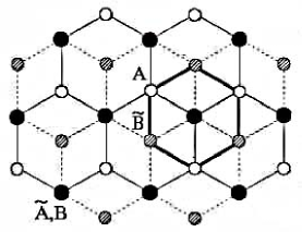
Figure 1: (Color online) Schematic of bilayer graphene lattice with AB (Bernal) stacking. Bonds in the bottom layer (A, B) are indicated by solid lines and in the top layer ($\widetilde{A}$, $\widetilde{B}$) by dash lines. A unit cell contains four atoms: A (white circles), $\widetilde{B}$ (gray), $\widetilde{A}$B dimer (solid).

We consider the bilayer graphene composed of two coupled hexagonal lattice including inequivalent sublattices $A$, $B$ on the bottom layer and $\widetilde{A}$, $\widetilde{B}$ on the top layer. The two layers are arranged in the AB (Bernal) stacking S. B. Trickey ; K. Yoshizawa , as shown in Fig. 1, where $B$ atoms are located directly below $\widetilde{A}$ atoms, and $A$ atoms are the centers of the hexagons in the other layer. The unit cell contains four atoms $A$, $B$, $\widetilde{A}$, and $\widetilde{B}$, and the Brillouin zone is identical with that of monolayer graphene. Here, the in-plane nearest-neighbor hopping integral between $A$ and $B$ atoms or between $\widetilde{A}$ and $\widetilde{B}$ atoms is denoted by $\gamma_{AB}=\gamma_{\widetilde{A}\widetilde{B}}=\gamma_{0}$. For the interlayer coupling, we take into account the largest hopping integral between $B$ and $\widetilde{A}$ atoms $\gamma_{\widetilde{A}B}=\gamma_{1}$, and the smaller hopping integral between $A$ and $\widetilde{B}$ atoms $\gamma_{A\widetilde{B}}=\gamma_{3}$. The values of these hopping integrals are estimated to be $\gamma_{0}=3.16$ eV W. W. Toy , $\gamma_{1}=0.39$ eV A. Misu , and $\gamma_{3}=0.315$ eV R. E. Doezema .

We assume that each monolayer graphene has totally $L_{y}$ zigzag chains with $L_{x}$ atomic sites on each chain Sheng . The size of the sample will be denoted as $N=L_{x}\times L_{y}\times L_{z}$, where $L_{z}=2$ is the number of monolayer graphene planes along the $z$ direction. In the presence of an applied magnetic field perpendicular to the plane of the bilayer graphene, the lattice model in real space can be written in the tight-binding form:

$$H = -\gamma_{0}\sum\limits_{\langle ij\rangle}e^{ia_{ij}}(c_{i}^{\dagger}c_{j}+\widetilde{c}_{i}^{\dagger}\widetilde{c}_{j})+(-\gamma_{1}\sum\limits_{\langle ij\rangle_{1}}e^{ia_{ij}}c_{jB}^{\dagger}\widetilde{c}_{i\widetilde{A}}$$ (1)

$$- \gamma_{3}\sum\limits_{\langle ij\rangle_{3}}e^{ia_{ij}}c_{iA}^{\dagger}\widetilde{c}_{j\widetilde{B}}+h.c.)+\sum\limits_{i}w_{i}(c_{i}^{\dagger}c_{i}+\widetilde{c}_{i}^{\dagger}\widetilde{c}_{i}),$$

where $c_{i}^{\dagger}$($c_{iA}^{\dagger}$), $c_{j}^{\dagger}$($c_{jB}^{\dagger}$) are creating operators on $A$ and $B$ sublattices in the bottom layer, and $\widetilde{c}_{i}^{\dagger}$($\widetilde{c}_{i\widetilde{A}}^{\dagger}$), $\widetilde{c}_{j}^{\dagger}$($\widetilde{c}_{j\widetilde{B}}^{\dagger}$) are creating operators on $\widetilde{A}$ and $\widetilde{B}$ sublattices in the top layer. The sum $\sum_{\langle ij\rangle}$ denotes the intralayer nearest-neighbor hopping in both layers, $\sum_{\langle ij\rangle_{1}}$ stands for interlayer hopping between the $B$ sublattice in the bottom layer and the $\widetilde{A}$ sublattice in the top layer, and $\sum_{\langle ij\rangle_{3}}$ stands for the interlayer hopping between the $A$ sublattice in the bottom layer and the $\widetilde{B}$ sublattice in the top layer, as described above. $w_{i}$ is a random disorder potential uniformly distributed in the interval $w_{i}\in[-W/2,W/2]\gamma_{0}$. The magnetic flux per hexagon $\phi=\sum_{{\small{\mbox{\hexagon}}}}a_{ij}=\frac{2\pi}{M}$, with $M$ an integer. The total flux through the sample is $N\frac{\phi}{2\pi}$, where $N=L_{x}L_{y}/M$ is taken to be an integer. When $M$ is commensurate with $L_{x}$ or $L_{y}$, the magnetic periodic boundary conditions are reduced to the ordinary periodic boundary conditions.

III III. Results and Discussion

The eigenstates $|\alpha\rangle$ and eigenenergies $\epsilon_{\alpha}$ of the system are obtained through exact diagonalization of the Hamiltonian Eq. (1), and the Hall conductivity $\sigma_{xy}$ is calculated by using the Kubo formula

$$\sigma_{xy}=\frac{ie^{2}\hbar}{S}\sum_{\alpha,\beta}\frac{\langle\alpha\mid V_{x}\mid\beta\rangle\langle\beta\mid V_{y}\mid\alpha\rangle-h.c.}{(\epsilon_{\alpha}-\epsilon_{\beta})^{2}},$$

where $S$ is the area of the sample, $V_{x}$ and $V_{y}$ are the velocity operators. In Fig. 2a, the Hall conductivity $\sigma_{xy}$ and electron density of states are plotted as functions of electron Fermi energy $E_{f}$ for a clean sample ($W=0$) at system size $N=96\times 24\times 2$ with magnetic flux $\phi=\frac{2\pi}{48}$, which illustrates the overall picture of the QHE in the full energy band. From the electron density of states, we can see the discrete LLs. We will call central LL at $E_{f}=0$ the $n=0$ LL, the one just above (below) it the $n=1$ ($n=-1$) LL, and so on. According to the behavior of $\sigma_{xy}$, the energy band is naturally divided into three different regimes. Around the band center, the Hall conductivity is quantized as $\sigma_{xy}=\nu\frac{e^{2}}{h}$, where $\nu=kg_{s}$ with $k$ an integer and $g_{s}=2$ for each LL due to double-valley degeneracy E. McCann ; Sheng (the spin degeneracy will contribute an additional factor $2$, which is omitted here). With each additional LL being occupied, the total Hall conductivity is increased by $g_{s}\frac{e^{2}}{h}$. This is an invariant as long as the states between the $n$-th and $(n-1)$-th LL are localized. $\sigma_{xy}=0$ at the particle-hole symmetric point $E_{f}=0$, which corresponds to the half-filling of the central LL. However, there is no $\sigma_{xy}=0$ quantized Hall plateau. These anomalously quantized Hall plateaus agree with the results observed experimentally in bilayer graphene K. S. Novoselov2 .

The Hall conductivity near the band edges, however, is quantized as $\sigma_{xy}=k\frac{e^{2}}{h}$ with $k$ an integer, as in the conventional QHE systems. Remarkably, around $E_{f}=\pm\gamma_{0}$ (within a narrow energy region $\Delta E\sim 0.4\gamma_{0}$), there are two critical regions which separate the unconventional and conventional QHE states, where the Hall conductance quantization is lost. These crossover regions also correspond to a novel transport regime, where the Hall resistance changes sign and the longitudinal conductivity exhibits metallic behavior. The singular behavior of the Hall conductivity in the crossover regions is likely to originate from the Van Hove singularity in the electron density of states at $B=0$ limit. In Fig. 2b, the quantization rule of the Hall conductivity in this unconventional region for three different strengths of magnetic flux is shown. With decreasing magnetic flux from $\phi=\frac{2\pi}{12}$ to $\frac{2\pi}{48}$, more quantized Hall plateaus emerge following the same quantization rule as the gap between the LLs is reduced.

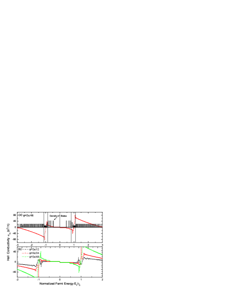
Figure 2: (Color online) (a) Calculated Hall conductivity and electron density of states in the full energy band for magnetic flux $\phi=\frac{2\pi}{48}$ or M=48, and (b) the Hall conductivity near the band center for $\phi=\frac{2\pi}{12}$, $\frac{2\pi}{24}$ and $\frac{2\pi}{48}$. The disorder strength is set to $W=0$ and $N=96\times 24\times 2$ in all cases. Inset: Hall conductivity at the band center. Here, the spin degrees of freedom are omitted, so $g_{s}=2$ and $g_{s}=1$ for the unconventional and conventional regions, respectively.

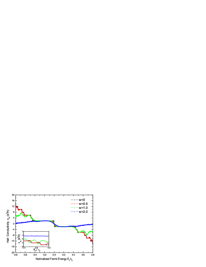
Figure 3: (Color online) Unconventional Hall conductivity as a function of electron Fermi energy near the band center for four different disorder strengths each averaged over $400$ disorder configurations. Inset: conventional Hall conductivity near the lower band edge. Here, $\phi=\frac{2\pi}{48}$ and the sample size is $N=96\times 24\times 2$.

Now we study the effect of random disorder on the unconventional QHE in bilayer graphene. In Fig. 3, the Hall conductivity around the band center is shown as a function of $E_{f}$ for four different disorder strengths at system size $N=96\times 24\times 2$ with magnetic flux $\phi=\frac{2\pi}{48}$. We can see that the plateaus with $\nu=\pm 10,\pm 6$ and $\pm 2$ remain well quantized at $W=0.5$. We mention that the $\nu=\pm 4,\pm 8$ plateaus are unclear at this relatively weak disorder strength because of very small plateau widths and relatively large localization lengths (the critical $W_{c}$ for each plateau will be obtained based on our larger size calculations of the Thouless number as presented later). With increasing $W$, higher Hall plateaus (with larger $|\nu|$) are destroyed first. At $W=2.0$, only the $\nu=\pm 2$ QHE remain robust. The last two plateaus $\nu=\pm 2$ eventually disappear around $W\sim 3.2$. For comparison, the QHE near the lower band edge is shown in the inset, where all plateaus disappear at a much weaker disorder strength $W\geq 1.0$. This clearly indicates that under the same conditions, the unconventional QHE around the band center is much more stable than the conventional QHE near the band edges. Clearly, after the destruction of the conventional QHE states near the band edge, these states become localized. Then the topological Chern numbers initially carried by these states will move towards band center in a similar manner to the single-layer graphene case Sheng . Thus we observe that the destruction of the unconventional QHE states near the band center is due to the float-up of extended levels.

Figure 4: (Color online) Calculated Hall conductivity with weaker magnetic flux $\phi=\frac{2\pi}{96}$, $\frac{2\pi}{192}$ and $\frac{2\pi}{288}$ for four different disorder strengths each averaged over $400$ disorder configurations. Here, the sample size is $N=96\times 24\times 2$.

To study the fate of the IQHE at weak magnetic field limit, we reduce the strength of magnetic field. In Fig. 4, the Hall conductivities around the band center with weaker magnetic flux $\phi=\frac{2\pi}{96}$, $\frac{2\pi}{192}$ and $\frac{2\pi}{288}$ are shown for different disorder strengths and system size $N=96\times 24\times 2$. In Fig. 4a, a lot more well quantized Hall plateaus emerge for a clean sample($W=0$), if we compare them with the results in Fig. 2b. In Fig. 4b, 4c and 4d, we can see that with the increasing of the disorder strength $W$, Hall plateaus are destroyed faster for the system with weaker magnetic flux $\phi$. At $W=2.0$, the most robust Hall plateaus at $\nu=\pm 2$ remain well quantized for magnetic flux $\phi=\frac{2\pi}{96}$ and $\frac{2\pi}{192}$, however, they already disappear for weaker magnetic flux $\phi=\frac{2\pi}{288}$. Our flux $2\pi/M$ in each hexagon the magnetic field is $B\sim 1.3\times 10^{5}/M$ Teslaweakb . Thus the weakest $B$ we used is about $451$ Tesla. This is a very large magnetic field comparing to the experimental ones around $B\sim 40$ Tesla. However, the topology of the QHE and how they disappear with the increase of the disorder strength $W$ remain to be the same as the stronger $B$ cases as demonstrated in Fig. 4a-4d. Thus, we establish that the obtained behavior of QHE for bilayer graphene will survive at weak $B$ limit.

We further investigate the quantum phase transition of the bilayer graphene electron system. In order to determine the critical disorder strength $W_{c}$ for the different QHE states, the Thouless number $g$ is calculated by using the following formula J.T.Edwards ,

$$g=\frac{\Delta E}{dE/dN}\ .$$

Here, $\Delta E$ is the geometric mean of the shift in the energy levels of the system caused by replacing periodic by antiperiodic boundary conditions, and $dE/dN$ is the mean spacing of the energy levels. The Thouless number $g$ is proportional to the longitudinal conductance $G$. In Fig. 5, we show some examples of calculated Thouless number for a relatively weak flux $\phi=\frac{2\pi}{48}$ and some different disorder strengths to explain how quantum phase transitions and the related phase boundaries $W_{c}$ are determined. In Fig. 5a, the calculated Thouless number $g$ and Hall conductivity $\sigma_{xy}$ as a function of $E_{f}$ at a weak disorder strength $W=0.2$ are plotted. Clearly, each valley in Thouless number corresponds to a Hall plateau and each peak corresponds to a critical point between two neighboring Hall plateaus. We can also call the first valley just above (below) $E_{f}=0$ the $\nu=-2$ ($\nu=2$) QHE state, the second one the $\nu=-4$ ($\nu=4$) state, and so on, as same as the Hall plateaus. In Fig. 5b-5d, we see that with increasing $W$, higher QHE states (valleys) are destroyed first. At $W=W_{c}=1.0$ (see Fig. 5b), the valleys with $\nu=\pm 12$ disappear, which correspond to the destruction of the $\nu=\pm 12$ Hall plateau states. Therefore, $W_{c}=1.0$ is the critical disorder strength, at which the $\nu=\pm 12$ plateau states change to an insulating phase. At $W=W_{c}=1.3$ (see Fig. 5c), the valleys with $\nu=\pm 8$ disappear, which indicates the destruction of the $\nu=\pm 8$ QHE states and their transition into the insulating phase. When $W=W_{c}=3.2$ (see Fig. 5d), the most stable QHE states with $\nu=\pm 2$ eventually disappear, which indicates all QHE phases are destroyed by disorder. All the phase boundaries $W_{c}$ between the different QHE states are determined in the same manner and tabulated in Table 1.

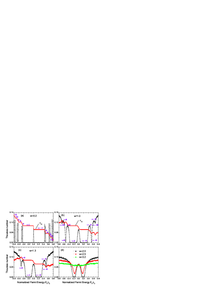
Figure 5: (Color online) (a)-(c) Calculated Thouless number and Hall conductivity for three different disorder strengths, and (d) Thouless number for other three disorder strengths, each data point being averaged over $400$ disorder configurations. Here, $\phi=\frac{2\pi}{48}$ and the sample size are taken to be $N=96\times 48\times 2$ and $N=96\times 24\times 2$ in the calculations of Thouless number and Hall conductivity, respectively.

We now focus on the region around $E_{f}=0$. In Fig. 6, we show the Thouless number for some different disorder strengths at system size $N=96\times 24\times 2$ and magnetic flux $\phi=\frac{2\pi}{48}$. We can see that the Thouless number shows a central peak at $E_{f}=0$. With increasing the disorder strength, the width of the peak increases and its height remains nearly unchanged. This behavior may suggest an interesting effect that the extended states originally sited at the critical point $E_{f}=0$ splits in the presence of disorder. However, the splitting is too small to induce two separated peaks in the Thouless number for the present sample sizes we can approach. Instead, it leads to a widened peak of unreduced height. This behavior also indicates that the critical longitudinal conductance in a small finite region near $E_{f}=0$ is almost constant about $2e^{2}/h$ according to the proportionality of Thouless number to longitudinal conductance. We have also confirmed this conclusion by direct Kubo formula calculation, in which the system size that can be approached is however much smaller.

Hall plateaus index	critical point $W_{c}$
$\nu=\pm 12$	1.0
$\nu=\pm 10$	1.2$\pm 0.1$
$\nu=\pm 8$	1.3$\pm 0.1$
$\nu=\pm 6$	1.6$\pm 0.1$
$\nu=\pm 4$	1.7$\pm 0.1$
$\nu=\pm 2$	3.2

Table 1: The phase boundaries $W_{c}$ for the different Hall plateaus.

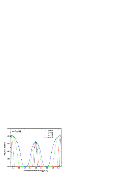
Figure 6: (Color online) (a) Thouless number for five different disorder strength, each point being averaged over $400$ disorder configurations. Here, $\phi=\frac{2\pi}{48}$ and the sample size is $N=96\times 48\times 2$.

IV IV. Summary

In summary, we have numerically investigated the QHE in bilayer graphene based on tight-binding model in the presence of disorder. The experimentally observed unconventional QHE is reproduced near the band center. The unconventional QHE plateaus around the band center are found to be much more stable than the conventional ones near the band edges. Our results of quantum phase transition indicate that with increasing disorder strength, the Hall plateaus can be destroyed through the float-up of extended levels toward the band center and higher plateaus always disappear first. At $W=W_{c}=3.2$, the most stable QHE states with $\nu=\pm 2$ eventually disappear, which indicates transition of all QHE phases into the insulating phase. A small critical region is observed between the $\nu=\pm 2$ plateaus, where the longitudinal conductance remains almost constant about $2e^{2}/h$ in the presence of moderate disorder, possibly due to the splitting of the critical point originally sited at $E_{f}=0$. We mention that in our numerical calculations, the magnetic field is much stronger than the ones one can realize in the experimental situation, as limited by current computational ability. However, the phase diagram we obtained is robust and applicable to weak field limit since it is determined by the topological property of the energy band as clearly established for single layer graphene Sheng and conventional quantum Hall systems Sheng0 . We further point out that the continuum model can not be used to address the fate of the quantum Hall effect in strong disorder or weak magnetic field limit. Because in such a model, both the band bottom and band edge are pushed to infinite energy limit, and thus one will not be able to see the important physics of opposite Chern numbers annihilating each other to destroy the IQHESheng .

Acknowledgment: This work is supported by the US DOE grant DE-FG02-06ER46305 (RS, DNS) and the NSF grant DMR-0605696 (RM, DNS). We thank the KITP for partial support through the NSF grant PHY05-51164. We also thank the partial support from the State Scholarship Fund from the China Scholarship Council, the Scientific Research Foundation of Graduate School of Southeast University of China (RM), the National Basic Research Program of China under grant Nos.: 2007CB925104 and 2009CB929504 (LS), and the NSF of China grant Nos.: 10874066 (LS), 10504011 (RS), 10574021 (ML), the doctoral foundation of Chinese Universities under grant No. 20060286044(ML).

References

- (1) K. S. Novoselov, A. K. Geim, S.V. Morozov, D. Jiang, M. I. Katsnelson, I.V. Grigorieva, S.V. Dubonos, and A. A. Firsov, Nature (London) 438, 197 (2005).
- (2) Y. Zhang, Y.-W. Tan, H. L.Stormer, and P. Kim, Nature (London) 438, 201 (2005).
- (3) J. Nilsson, A. H. Castro Neto, F. Guinea, and N. M. R. Peres, Phys. Rev. B 76, 165416 (2007).
- (4) E. McCann and V. I. Fal’ko, Phys. Rev. Lett. 96, 086805 (2006).
- (5) J. Nilsson, A. H. Castro Neto, N. M. R. Peres, and F. Guinea, Phys. Rev. B 73, 214418 (2006).
- (6) K. S. Novoselov, E. McCann, S. V. Morozov, V. I. Fal’ko, M. I. Katsnelson, U. Zeitler, D. Jiang, F. Schedin and A. K. Geim, Nature Phys. 2, 177 (2006).
- (7) J. G. Checkelsky, L. Li and N. P. Ong, Phys. Rev. Lett. 100, 206801 (2008).
- (8) Y. Hasegawa and M. Kohmoto, Phys. Rev. B 74, 155415 (2006).
- (9) D. A. Abanin, K. S. Novoselov, U. Zeitler, P. A. Lee, A. K. Geim and L. S. Levitov, Phys. Rev. Lett. 98, 196806 (2007).
- (10) E. V. Gorbar, V. P. Gusynin, V. A. Miransky and I. A. Shovkovy, Phys. Rev. B 78, 085437 (2008).
- (11) H. Min and A.H. MacDonald, Phys. Rev. B 77, 155416 (2008).
- (12) E. V. Castro, K. S. Novoselov, S. V. Morozov, N. M. R. Peres, J. M. B. Lopes dos Santos, J. Nilsson, F. Guinea, A. K. Geim, and A.H. Castro Neto, con-mat/08073348.
- (13) D. N. Sheng, L. Sheng, and Z. Y. Weng, Phys. Rev. B 73, 233406 (2006).
- (14) Y. Huo and R. N. Bhatt, Phys. Rev. Lett 68, 1375 (1992); D. N. Sheng, and Z. Y. Weng, ibid. 78, 318 (1997).
- (15) J. T. Edwards and D. J. Thouless, J. Phys. C 5, 807(1972); D. J. Thouless, Phys. Rep. 13C, 93 (1974).
- (16) S. B. Trickey, F. M .. u ller-Plathe, and G. H. F. Diercksen, Phys. Rev. B 45, 4460 (1992).
- (17) K. Yoshizawa, T. Kato, and T. Yamabe, J. Chem. Phys. 105, 2099 (1996); T. Yumura and K. Yoshizawa, Chem. Phys. 279, 111 (2002).
- (18) W. W. Toy, M. S. Dresselhaus, and G. Dresselhaus, Phys. Rev. B 15, 4077 (1977).
- (19) A. Misu, E. Mendez, and M. S. Dresselhaus, J. Phys. Soc. Jpn. 47, 199 (1979).
- (20) R. E. Doezema, W. R. Datars, H. Schaber, and A. Van Schyndel, Phys. Rev. B 19, 4224 (1979).
- (21) B. Bernevig, T. L. Hughes, H. Chen, C. Wu, S. C. Zhang, Inter. Jour. of Modern Phys. B 20, 3257 (2006).