Flavor Twisted Boundary Conditions and the Nucleon Vector Current

Abstract

Using flavor twisted boundary conditions, we study nucleon matrix elements of the vector current. We twist only the active quarks that couple to the current. Finite volume corrections due to twisted boundary conditions are determined using partially twisted, partially quenched, heavy baryon chiral perturbation theory, which we develop for the graded group $SU(7|5)$. Asymptotically these corrections are exponentially small in the volume, but can become pronounced for small twist angles. Utilizing the Breit frame does not mitigate volume corrections to nucleon vector current matrix elements. The derived expressions will allow for better controlled extractions of the isovector magnetic moment and the electromagnetic radii from simulations at zero lattice momentum. Our formalism, moreover, can be applied to any nucleon matrix elements.

I Introduction

Understanding QCD in the strongly interacting regime remains a challenging problem in physics. Simulations of QCD on Euclidean spacetime lattices are making progress towards a quantitative understanding of the non-perturbative dynamics in QCD DeGrand and DeTar (2006). Lattice QCD simulations usually employ periodic boundary conditions for the quark and gluon fields. Consequently the available hadron momenta are limited to periodic momentum modes of the lattice, $\bm{k}=2\pi\bm{n}/L$, where $\bm{n}$ is a triplet of integers and $L$ is the lattice size in each of the three spatial directions. On typical lattices, the smallest available lattice momentum is about $400-500\,\texttt{MeV}$. This presents a severe limitation for the study of observables appearing in matrix elements at low momentum, and low momentum-transfer. At present, such observables cannot be investigated directly using periodic boundary conditions, and models are used to perform momentum extrapolations.

For large enough volume, the physics should be independent of the choice of boundary conditions. There is freedom in choosing boundary conditions for fields; however, the action must be single valued so that observables are well-defined. For a generic matter field $\phi$, we can impose a twisted boundary condition in the $i$-th direction of the form, see e.g. Zinn-Justin (2002),

$$\phi(x_{i}+L)=U\,\phi(x_{i}),$$

where $U$ is a symmetry of the action and $U^{\dagger}U=1$. For the quark flavors in QCD, the diagonal flavor rotations can be used to implement what are called flavor-twisted boundary conditions. With $U$ of the form $U=\exp(i\theta_{i})$, the matter field $\phi$ has kinematic momentum $\bm{k}=(2\pi\bm{n}+\bm{\theta})/L$ which can be varied continuously by choosing different values for $\bm{\theta}$. The ability to produce continuous hadron momentum has made flavor-twisted boundary conditions attractive to lattice QCD Bedaque (2004); de Divitiis et al. (2004); Sachrajda and Villadoro (2005); Bedaque and Chen (2005); Tiburzi (2005a); Mehen and Tiburzi (2005); Flynn et al. (2005); Guadagnoli et al. (2006); Aarts et al. (2007); Tiburzi (2006); Jiang and Tiburzi (2007); Boyle et al. (2007); Simula (2007); Boyle et al. (2008); Jiang and Tiburzi (2008); Aoki et al. (2008).

In this work, we detail the finite volume modifications to nucleon form factors of the vector current. We use twisted boundary conditions on the active quarks in the current insertion, and, of course, are limited to only connected contributions from the current. Heavy baryon chiral perturbation theory is utilized to estimate the volume dependence of nucleon current matrix elements. Let us summarize our main findings.

• Finite volume modifications can be sizable especially for the magnetic contribution, and for small twist angles.

• The use of Breit frame kinematics does not dramatically reduce or simplify the finite volume corrections. The volume effect for magnetic observables in the Breit frame roughly doubles compared to the rest frame. This situation is unlike the meson vector current Jiang and Tiburzi (2008).

• With twisted boundary conditions on only the active quarks, the finite volume corrections depend on an unphysical and unknown parameter, $g_{1}$. This dependence arises as an artifact of the enlarged valence flavor group, and a lattice determination of $g_{1}$ would help in accounting for volume corrections.

• Results obtained here are qualitatively similar to those obtained from isospin-twisted boundary conditions for the nucleon isovector form factors Tiburzi (2006). In that method, valence $u$-quarks are twisted differently than the valence $d$-quarks without introducing extra fictitious flavors. We show, moreover, the flavor symmetry employed by that method can be used to eliminate the dependence on $g_{1}$. Consequently finite volume corrections can be reliably estimated for that case in terms of known low-energy constants.

Our presentation has the following organization. First in Section II, we detail the flavor twisted boundary conditions, and incorporate them into heavy baryon chiral perturbation theory. We show how the graded group $SU(7|5)$ accommodates twisting of the active valence quarks in the baryon sector. In Section III, we compute finite volume corrections to the nucleon mass, and derive the induced mass splittings due to flavor twisted boundary conditions. Numerically these splittings are estimated to be at the percent level or less on current lattices. Finite volume corrections to the vector form factors of the proton and neutron are determined in Section IV (complete expressions are given in Appendix A). These results apply to the connected contributions allowing access to isovector quantities, but not isoscalar. We show that terms arising from broken cubic invariance can lead to non-negligible volume effects in the region of small twist angles. Results for rest frame and Breit frame kinematics are compared. The Breit frame does not offer any substantial advantages with respect to volume effects. Complete results for isovector current matrix elements at finite volume using the method of isospin twisted boundary conditions are displayed in Appendix B. For rest frame kinematics, these results are shown to be independent of the unphysical parameter $g_{1}$. Appendix C collects functions and identities useful for the evaluation of finite volume effects. Finally a brief summary concludes our work.

II Flavor twisted boundary conditions and baryon chiral perturbation theory

To address the consequences of twisted boundary conditions in lattice calculations of baryon properties, we describe the underlying effective theory in the baryon sector. First we detail the partially twisted boundary conditions employed. Next we include these effects in chiral perturbation theory, and then heavy baryon chiral perturbation theory.

The quark part of the partially quenched QCD Lagrangian is given by

$$\mathcal{L}=\sum_{j,k=1}^{12}{\overline{\hat{Q}}}\,{}^{j}\left(D\hskip-6.49994pt/+m_{Q}\right)_{j}{}^{k}\,\hat{Q}_{k}.$$ (1)

The twelve quark fields transform in the fundamental representation of the graded group $SU(7|5)$, and appear in the vector $\hat{Q}^{\text{T}}=(\hat{u}_{0},\hat{u}_{1},\hat{u}_{2},\hat{d}_{1},\hat{d}_{2},\hat{j},\hat{l},\hat{\tilde{u}}_{0},\hat{\tilde{u}}_{1},\hat{\tilde{u}}_{2},\hat{\tilde{d}}_{1},\hat{\tilde{d}}_{2})$. In addition to the valence $\hat{u}_{0}$, $\hat{u}_{1}$, $\hat{u}_{2}$, $\hat{d}_{1}$, and $\hat{d}_{2}$ quarks, we have added their ghost quark counterparts $\hat{\tilde{u}}_{0}$, $\hat{\tilde{u}}_{1}$, $\hat{\tilde{u}}_{2}$, $\hat{\tilde{d}}_{1}$ and $\hat{\tilde{d}}_{2}$, which cancel the closed valence loops, and two sea quarks $\hat{j}$ and $\hat{l}$. In the isospin limit, the quark mass matrix of $SU(7|5)$ reads $m_{Q}=\text{diag}(m_{u}\bm{1}_{5\times 5},m_{j}\bm{1}_{2\times 2},m_{u}\bm{1}_{5\times 5})$ in block diagonal form, where the blocks correspond to valence, sea and ghost sectors. QCD quantities can be recovered in the limit $m_{j}\rightarrow m_{u}$. The additional up and down quarks are fictitious flavors differing only by their boundary conditions. There is one more up-type quark than down-type quark because we focus on a theory that will yield proton matrix elements. Neutron matrix elements can always be derived trivially by interchanging up and down charges in the final result.

The hats denote fields satisfying twisted boundary conditions. We require that the quark fields satisfy boundary conditions of the form

$$\hat{Q}(x+L\bm{e}_{r})=\exp\left(i\theta^{a}_{r}\,{\overline{T}}{}^{a}\right)\hat{Q}(x),$$ (2)

where $\bm{e}_{r}$ is a unit vector in the $r^{\text{th}}$ spatial direction, $L$ is the spatial size of the lattice, and the block diagonal form of the supermatrices ${\overline{T}}{}^{a}$ is

$${\overline{T}}{}^{a}=\text{diag}\left(T^{a},0,T^{a}\right).$$ (3)

Here we choose $T^{a}$ to be generators of the $U(5)$ Cartan subalgebra. Notice that by Eq. (3), the sea quarks remain periodic at the boundary. This reflects a partially twisted scenario. Twist angles can be changed without necessitating the generation of new gauge configurations, because the fermionic determinant, which arises solely from the sea sector, is not affected by the twisting.

Redefining the quark fields as $Q^{\text{T}}=(u_{0},u_{1},u_{2},d_{1},d_{2},j,l,\tilde{u}_{0},\tilde{u}_{1},\tilde{u}_{2},\tilde{d}_{1},\tilde{d}_{2})$, with $Q(x)=V^{\dagger}(x)\hat{Q}(x)$, where $V(x)=\exp(i\bm{{\theta}}^{a}\cdot\bm{x}\,{\overline{T}}{}^{a}/L)$, we can write the partially quenched QCD Lagrangian as

$${\mathcal{L}}=\sum_{j,k=1}^{12}{\overline{Q}}\,{}^{j}\left(\hat{D\hskip-6.49994pt/}+m_{Q}\right)_{j}{}^{k}\,Q_{k},$$ (4)

where all $Q$ fields satisfy periodic boundary conditions, and the effect of twisting has the form of a uniform gauge field: $\hat{D}_{\mu}=D_{\mu}+iB_{\mu}$, where $B_{\mu}=(\bm{{\theta}}^{a}\,{\overline{T}}{}^{a}/L,0)$. It will be easier to treat the twisting in the flavor basis of the valence and ghost sectors rather than in the generator basis, thus we write $\bm{{\theta}}^{a}\,T{}^{a}=\text{diag}(\bm{0},\bm{{\theta}}^{u},\bm{{\theta}^{\prime}}{}^{u},\bm{{\theta}}^{d},\bm{{\theta}^{\prime}}{}^{d})$, and similarly for $B_{\mu}$, which appears as $B_{\mu}=\text{diag}(B_{\mu}^{\text{val}},0,B_{\mu}^{\text{val}})$ in block diagonal form, with $B_{\mu}^{\text{val}}=\text{diag}(0,B^{u}_{\mu},B^{{}^{\prime}u}_{\mu},B^{d}_{\mu},B^{{}^{\prime}d}_{\mu})$. Momentum transfer will be generated using flavor changing currents from $u_{1}$ to $u_{2}$, or from $d_{1}$ to $d_{2}$. Notice we keep the $u_{0}$ quark periodic; it will play the role of spectator.

The low-energy effective theory of QCD is chiral perturbation theory, which describes the dynamics of pseudoscalar mesons emerging from spontaneous chiral symmetry breaking. The mesons of partially quenched chiral perturbation theory Bernard and Golterman (1994); Sharpe (1997); Golterman and Leung (1998); Sharpe and Shoresh (2000, 2001) are described by the coset field $\hat{\Sigma}$, which satisfies twisted boundary conditions. This field can be traded in for ${\Sigma}$, defined by ${\Sigma}(x)=V^{\dagger}(x)\hat{{\Sigma}}(x)V(x)$, which is periodic at the boundary Sachrajda and Villadoro (2005). In terms of this field, the Lagrangian of partially quenched chiral perturbation theory appears as

$${\mathcal{L}}=\frac{f^{2}}{8}\text{str}\left(\hat{D}_{\mu}{\Sigma}\hat{D}_{\mu}{\Sigma}^{\dagger}\right)-{\lambda}\,\text{str}\left(m_{Q}^{\dagger}{\Sigma}+{\Sigma}^{\dagger}m_{Q}\right)+\mu_{0}^{2}\Phi_{0}^{2}.$$ (5)

The action of the covariant derivative $\hat{D}^{\mu}$ is specified by $\hat{D}_{\mu}{\Sigma}=D_{\mu}{\Sigma}+i[B_{\mu},{\Sigma}]$. The parameter $f$ is the chiral limit value of the pion decay constant, and in our normalization, $f=0.13\,\texttt{GeV}$. The above Lagrangian contains only the lowest-order terms in an expansion in quark mass $m_{Q}$, and meson momentum $k^{2}$. The periodic meson fields contained in the twelve-by-twelve matrix $\phi$ are realized nonlinearly, ${\Sigma}=\exp(2i\phi/f)$. The matrix $\phi$ has the form

$$\phi=\begin{pmatrix}M_{vv}&M_{vs}&\chi^{\dagger}_{gv}\\ M_{sv}&M_{ss}&\chi^{\dagger}_{gs}\\ \chi_{gv}&\chi_{gs}&M_{gg}\end{pmatrix}.$$ (6)

The mesons of $M_{vv}$ ($M_{gg}$) are bosonic and are formed from a valence (ghost) quark-antiquark pair. These matrices have the form

$$M_{vv}=\begin{pmatrix}\eta^{u}_{00}&\eta^{u}_{01}&\eta^{u}_{02}&\pi^{+}_{01}&\pi^{+}_{02}\\ \eta^{u}_{10}&\eta^{u}_{11}&\eta^{u}_{12}&\pi^{+}_{11}&\pi^{+}_{12}\\ \eta^{u}_{20}&\eta^{u}_{21}&\eta^{u}_{22}&\pi^{+}_{21}&\pi^{+}_{22}\\ \pi^{-}_{10}&\pi^{-}_{11}&\pi^{-}_{12}&\eta^{d}_{11}&\eta^{d}_{12}\\ \pi^{-}_{20}&\pi^{-}_{21}&\pi^{-}_{22}&\eta^{d}_{21}&\eta^{d}_{22}\end{pmatrix},\,\,\text{and}\quad M_{gg}=\begin{pmatrix}\tilde{\eta}^{u}_{00}&\tilde{\eta}^{u}_{01}&\tilde{\eta}^{u}_{02}&\tilde{\pi}^{+}_{01}&\tilde{\pi}^{+}_{02}\\ \tilde{\eta}^{u}_{10}&\tilde{\eta}^{u}_{11}&\tilde{\eta}^{u}_{12}&\tilde{\pi}^{+}_{11}&\tilde{\pi}^{+}_{12}\\ \tilde{\eta}^{u}_{20}&\tilde{\eta}^{u}_{21}&\tilde{\eta}^{u}_{22}&\tilde{\pi}^{+}_{21}&\tilde{\pi}^{+}_{22}\\ \tilde{\pi}^{-}_{10}&\tilde{\pi}^{-}_{11}&\tilde{\pi}^{-}_{12}&\tilde{\eta}^{d}_{11}&\tilde{\eta}^{d}_{12}\\ \tilde{\pi}^{-}_{20}&\tilde{\pi}^{-}_{21}&\tilde{\pi}^{-}_{22}&\tilde{\eta}^{d}_{21}&\tilde{\eta}^{d}_{22}\end{pmatrix}.$$

The $\eta^{q}_{ij}$ ($\tilde{\eta}^{q}_{ij}$) mesons have quark content $\eta^{q}_{ij}\sim q_{i}{\overline{q}}_{j}$ ($\tilde{\eta}^{q}_{ij}\sim\tilde{q}_{i}\overline{\tilde{q}}_{j}$), while the $\pi^{+}_{ij}$ ($\tilde{\pi}^{+}_{ij}$) mesons have quark content $\pi^{+}_{ij}\sim u_{i}{\overline{d}}_{j}$ ($\tilde{\pi}^{+}_{ij}\sim\tilde{u}_{i}\overline{\tilde{d}}_{j}$ ). The valence-sea (sea-sea) mesons are bosonic and contained in $M_{vs}$ ($M_{ss}$) as

$$M_{sv}=\begin{pmatrix}\phi_{ju_{0}}&\phi_{ju_{1}}&\phi_{ju_{2}}&\phi_{jd_{1}}&\phi_{jd_{2}}\\ \phi_{lu_{0}}&\phi_{lu_{1}}&\phi_{lu_{2}}&\phi_{ld_{1}}&\phi_{ld_{2}}\end{pmatrix},\,\,\text{and}\quad M_{ss}=\begin{pmatrix}\eta_{j}&\pi_{jl}\\ \pi_{lj}&\eta_{l}\end{pmatrix}.$$

Mesons contained in $\chi_{gv}$ ($\chi_{gs}$) are built from ghost quark, valence antiquark (sea antiquark) pairs and are thus fermionic. These states appear as

$$\chi_{gv}=\begin{pmatrix}\phi_{\tilde{u}_{0}u_{0}}&\phi_{\tilde{u}_{0}u_{1}}&\phi_{\tilde{u}_{0}u_{2}}&\phi_{\tilde{u}_{0}d_{1}}&\phi_{\tilde{u}_{0}d_{2}}\\ \phi_{\tilde{u}_{1}u_{0}}&\phi_{\tilde{u}_{1}u_{1}}&\phi_{\tilde{u}_{1}u_{2}}&\phi_{\tilde{u}_{1}d_{1}}&\phi_{\tilde{u}_{1}d_{2}}\\ \phi_{\tilde{u}_{2}u_{0}}&\phi_{\tilde{u}_{2}u_{1}}&\phi_{\tilde{u}_{2}u_{2}}&\phi_{\tilde{u}_{2}d_{1}}&\phi_{\tilde{u}_{2}d_{2}}\\ \phi_{\tilde{d}_{1}u_{0}}&\phi_{\tilde{d}_{1}u_{1}}&\phi_{\tilde{d}_{1}u_{2}}&\phi_{\tilde{d}_{1}d_{1}}&\phi_{\tilde{d}_{1}d_{2}}\\ \phi_{\tilde{d}_{2}u_{0}}&\phi_{\tilde{d}_{2}u_{1}}&\phi_{\tilde{d}_{2}u_{2}}&\phi_{\tilde{d}_{2}d_{1}}&\phi_{\tilde{d}_{1}d_{2}}\end{pmatrix},\,\,\text{and}\quad\chi_{gs}=\begin{pmatrix}\phi_{\tilde{u}_{0}j}&\phi_{\tilde{u}_{0}l}\\ \phi_{\tilde{u}_{1}j}&\phi_{\tilde{u}_{1}l}\\ \phi_{\tilde{u}_{2}j}&\phi_{\tilde{u}_{2}l}\\ \phi_{\tilde{d}_{1}j}&\phi_{\tilde{d}_{1}l}\\ \phi_{\tilde{d}_{2}j}&\phi_{\tilde{d}_{2}l}\end{pmatrix}.$$

Expanding the Lagrangian in Eq. (5) to lowest order, one finds that mesons with quark content $Q\bar{Q^{\prime}}$ have mass

$$m_{QQ^{\prime}}^{2}=\frac{4{\lambda}}{f^{2}}(m_{Q}+m_{Q^{\prime}}).$$ (7)

Thus in infinite volume all mesons fall into one of three groups of mass degenerate states: valence-valence pions $m_{\pi}^{2}=8{\lambda}m_{u}/f^{2}$, valence-sea mesons $m_{ju}^{2}=4{\lambda}(m_{u}+m_{j})/f^{2}$, and sea-sea pions $m_{jj}^{2}=8{\lambda}m_{j}/f^{2}$. In partially quenched simulations, one measures the valence-valence and sea-sea pion masses. The valence-sea mass is given by the average of the other two, up to possible discretization errors that arise in hybrid actions.

The flavor singlet field, $\Phi_{0}=\frac{1}{\sqrt{2}}\text{str}\,\phi$, additionally acquires a mass $\mu_{0}$ which arises as a consequence of the $U(1)_{A}$ anomaly. Taking this mass to be large, the flavor singlet field is then integrated out of partially quenched chiral perturbation theory, however, the propagators of the flavor-neutral fields deviate from simple pole forms Sharpe and Shoresh (2000, 2001). There are two useful simplifications to note: twisted boundary conditions have no effect on the flavor neutral sector, and all valence-valence flavor neutral states are degenerate with mass $m_{\pi}$. For $a$,$b=u_{0}$, $u_{1}$, $u_{2}$, $d_{1}$, or $d_{2}$, the leading-order $\eta_{a}\eta_{b}$ propagator is thus given by

$${\cal G}_{\eta_{a}\eta_{b}}=\delta_{ab}\frac{1}{k^{2}+m_{\pi}^{2}}-\frac{1}{2}\frac{k^{2}+m^{2}_{jj}}{(k^{2}+m^{2}_{\pi})^{2}}.$$ (8)

The flavor neutral propagator can be conveniently rewritten as

$${\cal G}_{\eta_{a}\eta_{b}}=\frac{{\delta}_{ab}}{k^{2}+m_{\pi}^{2}}+{\cal H}_{ab}\left(\frac{1}{k^{2}+m_{\pi}^{2}}\right),$$ (9)

where

$${\cal H}_{ab}\left(A\right) = -\frac{1}{2}\left[1+(m_{\pi}^{2}-m_{jj}^{2})\frac{\partial}{\partial m_{\pi}^{2}}\right]A\,.$$ (10)

To include baryons into partially quenched chiral perturbation theory, one uses rank three flavor tensors Labrenz and Sharpe (1996); Savage (2002); Chen and Savage (2002); Beane and Savage (2002). In $SU(7|5)$, the spin-$\frac{1}{2}$ baryons are described by the $\bm{572}$-dimensional supermultiplet $\hat{{\mathcal{B}}}^{ijk}$, while the spin-$\frac{3}{2}$ baryons are described by the $\bm{300}$-dimensional supermultiplet $\hat{{\mathcal{T}}}_{\mu}^{ijk}$ Tiburzi (2005b). The baryon flavor tensors are twisted at the boundary of the lattice. In the $r^{\text{th}}$ spatial direction, both tensors satisfy boundary conditions of the form Tiburzi (2005a)

$$\hat{{\mathcal{B}}}_{ijk}(x+\hat{\bm{e}_{r}}L) = \left(e^{i\theta^{a}_{r}\,{\overline{T}}{}^{a}}\right)_{ii}\left(e^{i\theta^{a}_{r}\,{\overline{T}}{}^{a}}\right)_{jj}\left(e^{i\theta^{a}_{r}\,{\overline{T}}{}^{a}}\right)_{kk}\hat{{\mathcal{B}}}_{ijk}(x).$$ (11)

Thus we define new tensors ${\mathcal{B}}^{ijk}$ and ${\mathcal{T}}_{\mu}^{ijk}$ both having the form

$${\mathcal{B}}_{ijk}(x)=V^{\dagger}_{ii}(x)V^{\dagger}_{jj}(x)V^{\dagger}_{kk}(x)\hat{{\mathcal{B}}}_{ijk}(x).$$ (12)

These baryon fields satisfy periodic boundary conditions, and their free Lagrangian has the form

$${\mathcal{L}} = -i\left({\overline{{\mathcal{B}}}}v_{\mu}\hat{{\mathcal{D}}}_{\mu}{\mathcal{B}}\right)-2{\alpha}_{M}^{(PQ)}\left({\overline{{\mathcal{B}}}}{\mathcal{B}}{\mathcal{M}}_{+}\right)-2{\beta}_{M}^{(PQ)}\left({\overline{{\mathcal{B}}}}{\mathcal{M}}_{+}{\mathcal{B}}\right)-2\sigma_{M}^{(PQ)}\left({\overline{{\mathcal{B}}}}{\mathcal{B}}\right)\text{str}\left({\mathcal{M}}_{+}\right)$$

$$-i\left({\overline{{\mathcal{T}}}}_{\nu}v_{\mu}\hat{{\mathcal{D}}}_{\mu}{\mathcal{T}}_{\nu}\right)+{\Delta}\left({\overline{{\mathcal{T}}}}_{\nu}{\mathcal{T}}_{\nu}\right)+2{\gamma}_{M}^{(PQ)}\left({\overline{{\mathcal{T}}}}_{\nu}{\mathcal{M}}_{+}{\mathcal{T}}_{\nu}\right)+2{\overline{\sigma}}_{M}^{(PQ)}\left({\overline{{\mathcal{T}}}}_{\nu}{\mathcal{T}}_{\nu}\right)\text{str}\left({\mathcal{M}}_{+}\right),$$

where $v_{\mu}=(0,0,0,i)$ is the Euclidean four-velocity in the rest frame. The mass operator ${\mathcal{M}}_{+}$ is defined by ${\mathcal{M}}_{+}=\frac{1}{2}\left(\xi^{\dagger}m_{Q}\xi^{\dagger}+\xi m_{Q}\xi\right)$, with $\xi=\sqrt{{\Sigma}}$, and the covariant derivative acts on ${\mathcal{B}}$ and ${\mathcal{T}}_{\mu}$ fields in the same manner, namely

$$[\hat{{\mathcal{D}}}_{\mu}{\mathcal{B}}(x)]^{ijk}=[{\mathcal{D}}_{\mu}{\mathcal{B}}]^{ijk}(x)+i(B_{\mu}^{i}+B_{\mu}^{j}+B_{\mu}^{k}){\mathcal{B}}^{ijk}(x),$$ (14)

with

$$[{\mathcal{D}}_{\mu}{\mathcal{B}}]^{ijk}=\partial_{\mu}{\mathcal{B}}^{ijk}+(\hat{V}_{\mu})^{il}{\mathcal{B}}^{ljk}+(-)^{\eta_{i}(\eta_{j}+\eta_{l})}(\hat{V}_{\mu})^{jl}{\mathcal{B}}^{ilk}+(-)^{(\eta_{i}+\eta_{j})(\eta_{k}+\eta_{l})}(\hat{V}_{\mu})^{kl}{\mathcal{B}}^{ijl},$$ (15)

where the vector field of mesons $\hat{V}_{\mu}$ is given by $\hat{V}_{\mu}=\frac{1}{2}\left(\xi\hat{D}_{\mu}\xi^{\dagger}+\xi^{\dagger}\hat{D}_{\mu}\xi\right)$. This free Lagrangian contains a number of low-energy constants but has precisely the same form as in the $SU(4|2)$ partially quenched theory. Restricting the baryon multiplets to the sea sector, so that all flavor indices are either $6$ or $7$, we have nucleons and deltas made only of sea quarks. Hence the matching conditions are precisely the same as those used to match $SU(4|2)$ onto $SU(2)$ by restricting the former to the sea sector. The relations between the low-energy constants appearing in Eq. (LABEL:eq:LB) and those of $SU(2)$ chiral perturbation theory will not be needed here, but are given in Beane and Savage (2002).

The leading order partially quenched interaction Lagrangian between the baryons and mesons appears as

$${\mathcal{L}}=2{\alpha}\left({\overline{{\mathcal{B}}}}S_{\mu}{\mathcal{B}}\hat{A}_{\mu}\right)+2{\beta}\left({\overline{{\mathcal{B}}}}S_{\mu}\hat{A}_{\mu}{\mathcal{B}}\right)-2{\mathcal{H}}\left({\overline{{\mathcal{T}}}}_{\nu}S_{\mu}\hat{A}_{\mu}{\mathcal{T}}_{\nu}\right)+\sqrt{\frac{3}{2}}{\mathcal{C}}\left[\left({\overline{{\mathcal{T}}}}_{\nu}\hat{A}_{\nu}{\mathcal{B}}\right)+\left({\overline{{\mathcal{B}}}}\hat{A}_{\nu}{\mathcal{T}}_{\nu}\right)\right],$$ (16)

where the effects of partial twisting show up in the axial-vector field of mesons $\hat{A}_{\mu}=\frac{i}{2}\left(\xi\hat{D}_{\mu}\xi^{\dagger}-\xi^{\dagger}\hat{D}_{\mu}\xi\right)$. The interaction Lagrangian has the same form as the $SU(4|2)$ theory of baryons, hence the matching conditions to $SU(2)$ are identical. The familiar low-energy constants of $SU(2)$ are identified as follows Beane and Savage (2002): $g_{A}=\frac{2}{3}{\alpha}-\frac{1}{3}{\beta}$, $g_{{\Delta}N}=-{\mathcal{C}}$, and $g_{{\Delta}{\Delta}}={\mathcal{H}}$. Notice there is an extra free parameter in the partially quenched interaction Lagrangian compared to that of $SU(2)$ chiral peturbation theory. We shall write our expressions in terms of $g_{A}$ and the combination $g_{1}=\frac{1}{3}{\alpha}+\frac{4}{3}{\beta}$. Dependence on $g_{1}$ must drop out in the QCD limit, which, for the case at hand, requires both $m_{j}\to m_{u}$ and $L\to\infty$.

III Nucleon Mass

To begin, we determine the nucleon mass in the presence of partially twisted boundary conditions. In the isospin limit of $SU(4|2)$, the proton and neutron are degenerate Beane and Savage (2002); Tiburzi and Walker-Loud (2006). Flavor twisted boundary conditions, however, break the valence flavor symmetry, hence the nucleons are no longer degenerate. The nucleon mass splittings arise from finite volume effects induced by the boundary conditions. Effects of this type can be treated using chiral perturbation theory at finite volume. We work in the $p$-regime throughout, where $m_{\pi}L\gg 1$ so that zero modes of the pion field do not become strongly coupled Gasser and Leutwyler (1987); Leutwyler (1987); Gasser and Leutwyler (1988). We estimate the size of the mass splittings on current-sized lattices, and show that their effect can be neglected for the determination of nucleon observables using twisted boundary conditions.

In the infinite volume limit with $B_{\mu}$ held fixed, the nucleon mass is unaffected by the boundary conditions. This follows from a generalization of the argument presented for mesons in Sachrajda and Villadoro (2005). One merely realizes that the nucleon propagators are not boosted in heavy baryon chiral perturbation theory, because $v_{\mu}B_{\mu}=0$. The remaining momenta in a given diagram are mesonic, and are boosted according to flavor. Now since there are no flavor changing interactions, the sum of boosts at each vertex is zero. This, along with $v_{\mu}B_{\mu}=0$, assures us we can always shift loop momenta to cast any diagram into a form where the only $B$-dependence is that from external momenta. These contributions should be thought of as kinematical rather than effects which arise in the loops from chiral dynamics. The mass does not receive dynamical corrections from the boundary conditions, but the energy depends on the external momentum and has a kinematic dependence on the boundary conditions, e.g. for a nucleon with lattice momentum $\bm{k}$

$$E_{N}=M_{N}+\frac{(\bm{k}+\bm{B})^{2}}{2M_{N}}+\ldots,$$ (17)

where $\bm{B}=\bm{\theta}/L$, and $\ldots$ denotes terms that are higher order in $1/M_{N}$. Here only one valence quark in the nucleon has been twisted, and by an angle $\bm{\theta}$. When we try to apply the same reasoning at finite volume, no shifts of the internal momenta are possible because the loop momenta are discrete, while the twisting parameters are continuous. Thus there is a dynamical dependence on the twisting parameters arising from loops, and in finite volume, $M_{N}$ will depend upon $\bm{B}$.

Figure 1: Diagrams contributing to the nucleon mass and wavefunction renormalization in partially quenched chiral perturbation theory. A thin (thick) line denotes a spin-$1/2$ (spin-$3/2$) baryon, while a dashed line denotes a meson. Partially quenched hairpins are depicted by a crossed dashed line.

The mass of the nucleon in the chiral expansion can be written in the form

$$M_{N}=M_{0}(\mu)-M_{N}^{(1)}(\mu)-M_{N}^{(3/2)}(\mu)+\ldots,$$ (18)

where $\mu$ is the renormalization scale, and $M_{N}^{(n)}$ denotes the contribution to the nucleon mass of order $m_{q}^{n}$. The linear quark mass dependence arises from the local operators in Eq. (LABEL:eq:LB) at tree level, while the leading non-analytic contribution ${\mathcal{O}}(m_{q}^{3/2})$ arises from the one-loop diagrams shown in Figure 1. The local interactions do not contribute to finite volume effects, only the meson loops that are shown in the figure. For periodic boundary conditions, the finite volume effects on the nucleon mass have been determined in Beane (2004). To express the finite volume corrections to the nucleon mass with flavor twisted boundary conditions, we require the mode sum

$${\mathcal{K}}(m,\bm{B},{\Delta})=\int_{0}^{\infty}d{\lambda}\left[\frac{1}{L^{3}}\sum_{\bm{n}}\frac{(\bm{k}+\bm{B})^{2}}{[(\bm{k}+\bm{B})^{2}+{\beta}_{\Delta}^{2}]^{3/2}}-\int\frac{d\bm{k}}{(2\pi)^{3}}\frac{\bm{k}^{2}}{[\bm{k}^{2}+{\beta}_{\Delta}^{2}]^{3/2}}\right],$$ (19)

with ${\beta}_{\Delta}^{2}={\lambda}^{2}+2{\Delta}{\lambda}+m^{2}$, and $\bm{k}=2\pi\bm{n}/L$ where $\bm{n}$ is a triplet of integers. Evaluation of this function, as well as other finite volume sums, is discussed in Appendix A.

Consider purely valence nucleon states with exactly one twisted quark. These will be the only nucleons relevant in the computation of matrix elements with twisted boundary conditions. It is easiest to classify these states according to their representations under the valence subgroup of the two degenerate untwisted quarks. In our formulation, we must set the twist angles for these quarks to zero by hand. There is both a singlet, $\bm{1}$, and triplet, $\bm{3}$, representation for singly twisted nucleons under the untwisted valence $SU(2)$. For the mass of a nucleon with one twisted valence quark in the $\bm{3}$ representation, we find the finite volume shift ${\delta}M_{N_{\bm{3}}}(\bm{B})$ is given by

$${\delta}M_{N_{\bm{3}}}(\bm{B}) = -\frac{1}{2f^{2}}\Bigg{\{}g_{\pi N_{\bm{3}}N_{\bm{3}}}^{2}{\mathcal{K}}(m_{\pi},\bm{0},0)+g_{\pi N_{\bm{3}}N_{\bm{3}}}^{\prime\,2}{\mathcal{K}}(m_{\pi},\bm{B},0)+g_{juN_{\bm{3}}N_{\bm{3}}}^{2}{\mathcal{K}}(m_{ju},\bm{0},0)$$

$$\phantom{spacer.}+g_{juN_{\bm{3}}N_{\bm{3}}}^{\prime\,2}{\mathcal{K}}(m_{ju},\bm{B},0)+(g_{A}+g_{1})^{2}{\mathcal{H}}_{uu}\Big{(}{\mathcal{K}}(m_{\pi},\bm{0},0)\Big{)}$$

$$\phantom{}+\frac{1}{9}g_{{\Delta}N}^{2}\Bigg{[}{\mathcal{K}}(m_{\pi},\bm{0},{\Delta})+5{\mathcal{K}}(m_{\pi},\bm{B},{\Delta})+2{\mathcal{K}}(m_{ju},\bm{0},{\Delta})+4{\mathcal{K}}(m_{ju},\bm{B},{\Delta})\Bigg{]}\Bigg{\}}.$$

The effective axial couplings are defined by

$$g_{\pi N_{\bm{3}}N_{\bm{3}}}^{2} = \frac{1}{3}(g_{A}^{2}+2g_{A}g_{1}+g_{1}^{2}/4),$$

$$g_{\pi N_{\bm{3}}N_{\bm{3}}}^{\prime\,2} = \frac{1}{3}(g_{A}^{2}-g_{A}g_{1}-5g_{1}^{2}/4),$$

$$g_{juN_{\bm{3}}N_{\bm{3}}}^{2} = \frac{1}{3}(4g_{A}^{2}+2g_{A}g_{1}+g_{1}^{2}),$$

$$g_{juN_{\bm{3}}N_{\bm{3}}}^{\prime\,2} = \frac{1}{2}g_{1}^{2}.$$ (21)

On the other hand, for a nucleon in the $\bm{1}$ representation, we find the finite volume shift ${\delta}M_{N_{\bm{1}}}(\bm{B})$ given by

$${\delta}M_{N_{\bm{1}}}(\bm{B}) = -\frac{1}{2f^{2}}\Bigg{\{}g_{\pi N_{\bm{1}}N_{\bm{1}}}^{2}{\mathcal{K}}(m_{\pi},\bm{0},0)+g_{\pi N_{\bm{1}}N_{\bm{1}}}^{\prime\,2}{\mathcal{K}}(m_{\pi},\bm{B},0)+g_{juN_{\bm{1}}N_{\bm{1}}}^{2}{\mathcal{K}}(m_{ju},\bm{0},0)$$ (22)

$$\phantom{spacer.}+g_{juN_{\bm{1}}N_{\bm{1}}}^{\prime\,2}{\mathcal{K}}(m_{ju},\bm{B},0)+(g_{A}+g_{1})^{2}{\mathcal{H}}_{uu}\Big{(}{\mathcal{K}}(m_{\pi},\bm{0},0)\Big{)}$$

$$\phantom{sp}+\frac{1}{3}g_{{\Delta}N}^{2}\Bigg{[}{\mathcal{K}}(m_{\pi},\bm{0},{\Delta})+{\mathcal{K}}(m_{\pi},\bm{B},{\Delta})+2{\mathcal{K}}(m_{ju},\bm{0},{\Delta})\Bigg{]}\Bigg{\}}.$$

The effective axial couplings for the singlet nucleon mass are defined by

$$g_{\pi N_{\bm{1}}N_{\bm{1}}}^{2} = \frac{1}{9}(g_{A}^{2}-4g_{A}g_{1}-11g_{1}^{2}/4),$$

$$g_{\pi N_{\bm{1}}N_{\bm{1}}}^{\prime\,2} = \frac{1}{9}(5g_{A}^{2}+7g_{A}g_{1}-g_{1}^{2}/4),$$

$$g_{juN_{\bm{1}}N_{\bm{1}}}^{2} = \frac{1}{9}(4g_{A}^{2}+2g_{A}g_{1}+7g_{1}^{2}),$$

$$g_{juN_{\bm{1}}N_{\bm{1}}}^{\prime\,2} = \frac{1}{9}(8g_{A}^{2}+4g_{A}g_{1}+g_{1}^{2}/2).$$ (23)

In the limit $\bm{B}=\bm{0}$, there is no difference between the representations, and we recover accordingly the finite volume shift of the partially quenched nucleon mass Beane (2004). In the rest of this section, we work for simplicity at the unitary mass point $m_{j}=m_{u}$, so that $m_{ju}^{2}=m_{\pi}^{2}$.

We consider nucleon splittings for two cases that are of interest in current matrix elements: rest frame kinematics, and Breit frame kinematics. In the rest frame kinematics, the initial nucleon is at rest, and hence completely untwisted. The final nucleon has been given a boost by twisting one of the quarks by $\bm{\theta}$. In this case, there are three mass splittings among the various nucleons: that between the $\bm{3}$ and untwisted nucleon, that between the $\bm{1}$ and untwisted nucleon, and that between the $\bm{3}$ and $\bm{1}$ nucleons. The relative change in these splittings is given by

$${\Delta}M_{\bm{3}} \equiv \frac{M_{N_{\bm{3}}}(\bm{B})-M_{N}}{M_{N}}$$ (25)

$$= -\frac{1}{2f^{2}M_{N}}\Bigg{\{}\frac{1}{3}(g_{A}^{2}-g_{A}g_{1}+g_{1}^{2}/4)\Big{[}{\mathcal{K}}(m_{\pi},\bm{B},0)-{\mathcal{K}}(m_{\pi},\bm{0},0)\Big{]}$$

$$\phantom{space}+g_{{\Delta}N}^{2}\Big{[}{\mathcal{K}}(m_{\pi},\bm{B},{\Delta})-{\mathcal{K}}(m_{\pi},\bm{0},{\Delta})\Big{]}\Bigg{\}},$$

$${\Delta}M_{\bm{1}} \equiv \frac{M_{N_{\bm{1}}}(\bm{B})-M_{N}}{M_{N}}$$ (27)

$$= -\frac{1}{2f^{2}M_{N}}\Bigg{\{}\frac{1}{9}(13g_{A}^{2}+11g_{A}g_{1}+g_{1}^{2}/4)\Big{[}{\mathcal{K}}(m_{\pi},\bm{B},0)-{\mathcal{K}}(m_{\pi},\bm{0},0)\Big{]}$$

$$\phantom{space}+\frac{1}{3}g_{{\Delta}N}^{2}\Big{[}{\mathcal{K}}(m_{\pi},\bm{B},{\Delta})-{\mathcal{K}}(m_{\pi},\bm{0},{\Delta})\Big{]}\Bigg{\}},$$

and

$${\Delta}M_{\bm{3}-\bm{1}} \equiv \frac{M_{N_{\bm{3}}}(\bm{B})-M_{N_{\bm{1}}}(\bm{B})}{M_{N}}$$ (29)

$$= -\frac{1}{2f^{2}M_{N}}\Bigg{\{}-\frac{1}{9}(10g_{A}^{2}+14g_{A}g_{1}-g_{1}^{2}/2)\Big{[}{\mathcal{K}}(m_{\pi},\bm{B},0)-{\mathcal{K}}(m_{\pi},\bm{0},0)\Big{]}$$

$$\phantom{space}+\frac{2}{3}g_{{\Delta}N}^{2}\Big{[}{\mathcal{K}}(m_{\pi},\bm{B},{\Delta})-{\mathcal{K}}(m_{\pi},\bm{0},{\Delta})\Big{]}\Bigg{\}},$$

respectively.

On the other hand, for the Breit frame kinematics the initial state nucleon has one quark twisted by $\bm{\theta}$, while the final state nucleon has one quark twisted by $-\bm{\theta}$. The finite volume modification given by the function ${\mathcal{K}}(m,\bm{B},{\Delta})$ in Eq. (19) is even with respect to $\bm{B}$. Thus initial and final state nucleons in the same representation of the untwisted $SU(2)$ are degenerate. The only non-vanishing splitting is between the different representations, but on account of evenness in $\bm{B}$, this splitting is identical to ${\Delta}M_{\bm{3}-\bm{1}}$ given above in Eq. (29).

             

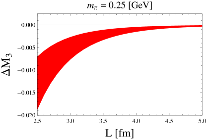
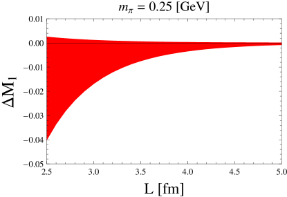
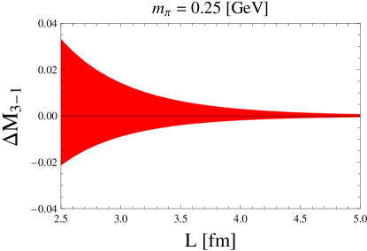
Figure 2: Numerical estimates for the maximal nucleon splittings at finite volume, ${\Delta}M_{\bm{3}}$, ${\Delta}M_{\bm{1}}$, and ${\Delta}M_{\bm{3}-\bm{1}}$ given in Eqs. (25), (27), and (29), respectively. We plot each relative splitting as a function of $L$ with the lattice pion mass fixed at $m_{\pi}=0.25\,\texttt{GeV}$. The twist angles are fixed at $\bm{\theta}=\pi(1,1,1)$ to give the maximal splittings. The bands arise from variation of the parameter $g_{1}$ assuming naturalness.

Numerically we can estimate the nucleon splittings by using phenomenological input for the low-energy constants: $g_{A}=1.25$, $g_{{\Delta}N}=1.5$, ${\Delta}=0.29\,\texttt{GeV}$, $M_{N}=0.94\,\texttt{GeV}$, and $f=0.13\,\texttt{GeV}$. For the unknown partially quenched axial coupling $g_{1}$, we assume it is of natural size and vary it within the rage $-2\leq g_{1}\leq 2$. Each of the mass splittings ${\Delta}M_{\bm{3}}$, ${\Delta}M_{\bm{1}}$, and ${\Delta}M_{\bm{3}-\bm{1}}$ is a maximum when $\bm{\theta}=\pi(1,1,1)$. We choose this value for $\bm{\theta}$ to investigate the worst case scenario. In Figure 2, we investigate the relative mass splittings’ dependence on $L$ for a fixed value of $m_{\pi}$, which is chosen to be $0.25\,\texttt{GeV}$. Values shown for the maximal splittings are all less than five percent. We will thus neglect the nucleon splittings in our analysis below.

IV Nucleon isovector form factors

Electromagnetic form factors appear in vector current matrix elements of the nucleon. In terms of Dirac and Pauli form factors denoted by $F_{1}^{N}(\bm{Q}^{2})$ and $F_{2}^{N}(\bm{Q}^{2})$, respectively, the nucleon current matrix element has the decomposition

$$\langle N(\bm{P}^{\prime})|J^{\text{em}}_{\mu}|N(\bm{P})\rangle={\overline{u}}(\bm{P}^{\prime})\left[\gamma_{\mu}F^{N}_{1}(\bm{Q}^{2})-\frac{\sigma_{\mu\nu}Q_{\nu}}{2M_{N}}F^{N}_{2}(\bm{Q}^{2})\right]u(\bm{P}),$$ (30)

where $Q_{\mu}=(P^{\prime}-P)_{\mu}$ is the momentum transfer. In QCD, the electromagnetic current is given as $J^{\text{em}}_{\mu}=q_{u}\,{\overline{u}}\gamma_{\mu}u+q_{d}\,{\overline{d}}\gamma_{\mu}d$. In heavy baryon chiral perturbation theory, the decomposition of the current appears in terms of the Sachs electric and magnetic form factors, $G_{E}^{N}(\bm{Q}^{2})$ and $G_{M}^{N}(\bm{Q}^{2})$, i.e. one has

$$\langle N_{v}(\bm{P}^{\prime})|J^{\text{em}}_{\mu}|N_{v}(\bm{P})\rangle={\overline{u}}_{v}\left[v_{\mu}G^{N}_{E}(\bm{Q}^{2})-\frac{[S_{\mu},S_{\nu}]Q_{\nu}}{M_{N}}G^{N}_{M}(\bm{Q}^{2})\right]u_{v},$$ (31)

with the relations

$$G_{E}^{N}(\bm{Q}^{2}) = F_{1}^{N}(\bm{Q}^{2})+\frac{Q^{2}}{4M_{N}^{2}}F_{2}^{N}(\bm{Q}^{2})$$ (32)

$$G_{M}^{N}(\bm{Q}^{2}) = F_{1}^{N}(\bm{Q}^{2})+F^{N}_{2}(\bm{Q}^{2}).$$ (33)

We have appended velocity subscripts in Eq. (31) for clarity. The $u_{v}$ are two-component Pauli spinors.

To calculate these form factors with twisted boundary conditions on the lattice, one writes the current matrix element in terms of the various quark contractions with the electromagnetic current. The propagators coupling to the current in each contraction we call the active quark propagators. These are the propagators determined with twisted boundary conditions. Omitted from this calculation are the current insertions on quark lines that are self-contracted. These disconnected contributions are notoriously difficult to calculate using lattice QCD. This difficulty notwithstanding, their contributions cannot be modified to produce continuous momentum transfer between the initial and final state hadron. As with present-day lattice calculations, we too will omit these contributions but with the caveat that their eventual inclusion will be limited to hadrons with Fourier momentum modes of the lattice.

Now we discuss precisely how to calculate the connected part of the nucleon form factors in the effective theory. To specialize to the application of twisted boundary conditions on the active quarks, we must separate the current into two pieces,

$$J_{\mu}^{1} = q_{u}\,{\overline{u}}_{2}\gamma_{\mu}u_{1}$$ (34)

$$J_{\mu}^{2} = q_{d}\,{\overline{d}}_{2}\gamma_{\mu}d_{1}.$$ (35)

By evaluating matrix elements of $J_{\mu}^{1}$ with $\bm{\theta}^{u}=\bm{\theta}$, $\bm{\theta^{\prime}}^{u}=\bm{\theta^{\prime}}$, and $J_{\mu}^{2}$ with $\bm{\theta}^{d}=\bm{\theta}$, $\bm{\theta^{\prime}}^{d}=\bm{\theta^{\prime}}$, both currents induce momentum transfer from $\bm{P}=\bm{\theta}/L$ to $\bm{P}^{\prime}=\bm{\theta^{\prime}}/L$. First let us consider proton matrix elements. Considering the quark-level contractions, we find

$$\frac{3}{2}\big{\langle}N_{\bm{1}}(uu_{2}d_{1})\big{|}J_{\mu}^{1}\big{|}N_{\bm{1}}(uu_{1}d_{1})\big{\rangle}\Bigg{|}_{\bm{\theta}^{d}=\bm{0}}+\frac{1}{2}\big{\langle}N_{\bm{3}}(uu_{2}d_{1})\big{|}J_{\mu}^{1}\big{|}N_{\bm{3}}(uu_{1}d_{1})\big{\rangle}\Bigg{|}_{\bm{\theta}^{d}=\bm{0}}\\ +\big{\langle}N_{\bm{3}}(uud_{2})\big{|}J_{\mu}^{2}\big{|}N_{\bm{3}}(uud_{1})\big{\rangle}\overset{L\to\infty}{\longrightarrow}\langle p(\bm{P}^{\prime})|J_{\mu}^{\text{em}}|p(\bm{P})\rangle_{\text{connected}}.$$ (36)

The subscripts on $N$ refer to the representation under untwisted isospin, and parenthetically we list the quark content. We treat the active quark twists as implicit: each is from an initial quark, $u_{1}$ or $d_{1}$, with twist $\bm{\theta}$ to a final quark, $u_{2}$ or $d_{2}$, with twist $\bm{\theta^{\prime}}$. We stress that Eq. (36) provides the recipe for calculating in the effective theory what is implemented on the lattice by twisting the active quarks. For the neutron there is a similar construction, however, it is easiest to appeal to charge symmetry (isospin rotation by $\pi/2$) from which follows the relation

$$\langle n(\bm{P}^{\prime})|J_{\mu}^{\text{em}}|n(\bm{P})\rangle=\langle p(\bm{P}^{\prime})|J_{\mu}^{\text{em}}|p(\bm{P})\rangle\Bigg{|}_{q_{u}\leftrightarrow q_{d}}.$$ (37)

In partially quenched QCD, the current is defined by $J^{a}_{\mu}={\overline{Q}}\gamma_{\mu}{\overline{{\mathcal{Q}}}}{}^{a}Q$. The choice of supermatrices ${\overline{{\mathcal{Q}}}}{}^{a}$ used to extend the charges is not unique Golterman and Pallante (2001). One should choose a form of the supermatrices that maintains the cancellation of valence and ghost quark loops with an operator insertion Tiburzi (2005c). For the flavor changing currents we consider, the simplest choice $({\overline{{\mathcal{Q}}}}{}^{1})_{ij}=q_{u}\,\delta_{i3}\,\delta_{j2}$ and $({\overline{{\mathcal{Q}}}}{}^{2})_{ij}=q_{d}\,\delta_{i5}\,\delta_{j4}$ results in the correct physics. This is because operator self-contractions automatically vanish; thus, any non-zero charges in the ghost sector must ultimately yield zero, and consequently would be superfluous. Charges in the sea, while not superfluous, are absent due to restricting to the connected part of three-point functions.

Operators that contribute at tree-level to the electromagnetic currents in $SU(2)$ chiral perturbation theory are contained in the Lagrangian

$${\mathcal{L}} = -\frac{i\mu_{0}}{2M_{N}}\left({\overline{N}}[S_{\mu},S_{\nu}]N\right)\text{tr}({\mathcal{Q}})F_{\mu\nu}-\frac{i\mu_{I}}{2M_{N}}\left({\overline{N}}[S_{\mu},S_{\nu}]{\mathcal{Q}}N\right)F_{\mu\nu}$$ (38)

$$-\frac{c_{0}}{{\Lambda}_{\chi}^{2}}\left({\overline{N}}N\right)\text{tr}({\mathcal{Q}})v_{\mu}\partial_{\nu}F_{\mu\nu}-\frac{c_{I}}{{\Lambda}_{\chi}^{2}}\left({\overline{N}}{\mathcal{Q}}N\right)v_{\mu}\partial_{\nu}F_{\mu\nu},$$

where ${\mathcal{Q}}=\text{diag}(q_{u},q_{d})$ is the electric charge matrix. The operators with coefficients $\mu_{0}$ and $\mu_{I}$ give the leading local contributions to the magnetic moments, while the operators with coefficients $c_{0}$ and $c_{I}$ give the leading local contributions to the electric charge radii. Operators for the magnetic radii occur at one higher order than the leading loop contributions. The combination $\frac{2}{3}\mu_{0}+\frac{1}{3}\mu_{I}$ is isoscalar, while $\mu_{I}$ is isovector. Analogous linear combinations of $c_{0}$ and $c_{I}$ form isoscalar and isovector contributions to the charge radius. In writing down the analogous terms in the partially quenched chiral Lagrangian, ${\mathcal{Q}}\to{\overline{{\mathcal{Q}}}}{}^{a}$. Because of the condition $\text{str}({\overline{{\mathcal{Q}}}}{}^{a})=0$, we see that there will be missing information in the partially quenched theory: there will only be operators where ${\overline{{\mathcal{Q}}}}{}^{a}$ transforms under the adjoint, because of the lack of singlet component. This is the effective theory manifestation of neglecting the disconnected contributions. Consequently we will not be sensitive to the isoscalar combination low-energy constants.

To consider the baryon current in partially twisted, partially quenched chiral perturbation theory, we promote ${\overline{{\mathcal{Q}}}}{}^{a}$ from the specific form used in our calculations to the most general form transforming under both the adjoint and singlet of $SU(7|5)$. The baryon current has the form

$${\delta}J^{a}_{\mu} = -\frac{i}{2M_{N}}\left\{\mu_{\alpha}\hat{D}_{\nu}\left({\overline{{\mathcal{B}}}}[S_{\mu},S_{\nu}]{\mathcal{B}}{\overline{{\mathcal{Q}}}}{}^{a}\right)+\mu_{\beta}\hat{D}_{\nu}\left({\overline{{\mathcal{B}}}}[S_{\mu},S_{\nu}]{\overline{{\mathcal{Q}}}}{}^{a}{\mathcal{B}}\right)+\mu_{\gamma}\hat{D}_{\nu}\left({\overline{{\mathcal{B}}}}[S_{\mu},S_{\nu}]{\mathcal{B}}\right)\,\text{str}({\overline{{\mathcal{Q}}}}{}^{a})\right\}$$ (39)

$$-\frac{1}{{\Lambda}_{\chi}^{2}}\Bigg{\{}c_{\alpha}\left[\hat{D}_{\mu}\hat{D}_{\nu}\left({\overline{{\mathcal{B}}}}v_{\nu}{\mathcal{B}}{\overline{{\mathcal{Q}}}}{}^{a}\right)-\hat{D}^{2}\left({\overline{{\mathcal{B}}}}v_{\nu}{\mathcal{B}}{\overline{{\mathcal{Q}}}}{}^{a}\right)\right]+c_{\beta}\left[\hat{D}_{\mu}\hat{D}_{\nu}\left({\overline{{\mathcal{B}}}}v_{\nu}{\overline{{\mathcal{Q}}}}{}^{a}{\mathcal{B}}\right)-\hat{D}^{2}\left({\overline{{\mathcal{B}}}}v_{\nu}{\overline{{\mathcal{Q}}}}{}^{a}{\mathcal{B}}\right)\right]$$

$$\phantom{spacers}+c_{\gamma}\left[\hat{D}_{\mu}\hat{D}_{\nu}\left({\overline{{\mathcal{B}}}}v_{\nu}{\mathcal{B}}\right)-\hat{D}^{2}\left({\overline{{\mathcal{B}}}}v_{\nu}{\mathcal{B}}\right)\right]\,\text{str}({\overline{{\mathcal{Q}}}}{}^{a})\Bigg{\}}.$$

Restricting all quark indices in Eq. (39) to the sea sector, we can match onto the nucleon current of two-flavor chiral perturbation theory in Eq. (38). Matching with the physical light quark charges yields the relations

$$\mu_{0}=\frac{1}{6}\mu_{\alpha}+\frac{2}{3}\mu_{\beta}+\mu_{\gamma}, \mu_{I}=\frac{2}{3}\mu_{\alpha}-\frac{1}{3}\mu_{\beta},$$ (40)

$$c_{0}=\frac{1}{6}c_{\alpha}+\frac{2}{3}c_{\beta}+c_{\gamma}, c_{I}=\frac{2}{3}c_{\alpha}-\frac{1}{3}c_{\beta},$$ (41)

between the partially quenched low-energy constants and the physical parameters of chiral perturbation theory. Because our current lacks a flavor singlet component, $\text{str}({\overline{{\mathcal{Q}}}}{}^{a})=0$, the constants $\mu_{\gamma}$ and $c_{\gamma}$ will always be absent from our expressions for nucleon current matrix elements. Consequently only the isovector combinations will be expressible in terms of physical parameters, specifically $\mu_{I}$ and $c_{I}$. The isoscalar combinations will always contain unphysical low-energy constants even at the unitary mass point $m_{j}=m_{u}$.

IV.1 Infinite Volume

A useful check on our formulation of current matrix elements for partially twisted boundary conditions is the infinite volume limit. In this limit, we must recover the connected parts of the proton and neutron form factors. These results, moreover, show the consequences of vanishing sea quark charges, and are of use to lattice practitioners beyond the use of twisted boundary conditions.

The calculation of the current matrix elements in Eq. (36) can be split into two parts. There are local contributions and loop contributions. The local terms are easiest: there are Born level charge couplings contained in the free Lagrangian (LABEL:eq:LB), and there are additional local contributions from higher-order operators appearing in the baryon current (39). The loop contributions are generated from the pion-nucleon-nucleon and pion-nucleon-delta interactions contained in the Lagrangian Eq. (16). The relevant diagrams are depicted in Figure 3. Additionally at this order, we need to multiply the Born-level couplings by the wavefunction renormalization which arises from the diagrams in Figure 1.

Figure 3: Diagrams contributing to the nucleon vector current in partially quenched chiral perturbation theory. A thin (thick) line denotes a spin-$1/2$ (spin-$3/2$) baryon, while a dashed line denotes a meson. Partially quenched hairpins are depicted by a crossed dashed line and the wiggly line represents the vector current.

To express the form factors, we define the three momentum transfer $\bm{Q}=\bm{q}+\bm{B}^{\prime}-\bm{B}$, and the quantity

$$P_{\phi}=\sqrt{1+\frac{x(1-x)\bm{Q}^{2}}{m_{\phi}^{2}}}.$$ (42)

Here we are additionally considering the nucleon with Fourier momentum transfer $\bm{q}=2\pi\bm{n}/L$, where $\bm{n}$ is a triplet of integers. Expressing the form factors in terms of $\bm{Q}$, we can easily generalize between the untwisted case $\bm{B}=\bm{B}^{\prime}=\bm{0}$, and the case of zero lattice momentum $\bm{q}=\bm{0}$. In infinite volume, all results can be expressed as a function of $\bm{Q}$.

For the proton, the local and loop contributions produce the connected part of the electric form factor

$$G_{E}^{p}(\bm{Q}^{2}) = 2q_{u}+q_{d}+\frac{\bm{Q}^{2}}{6{\Lambda}_{\chi}^{2}}\left[\ q_{u}(5c_{\alpha}+2c_{\beta})+q_{d}(c_{\alpha}+4c_{\beta})\right]$$

$$+\frac{2}{(4\pi f)^{2}}\int_{0}^{1}dx\,(2q_{u}+q_{d})\left\{\frac{1}{6}\bm{Q}^{2}\log\frac{m^{2}_{ju}}{\mu^{2}}+m_{ju}^{2}P_{ju}^{2}\log P_{ju}^{2}\right\}$$

$$+\frac{1}{(4\pi f)^{2}}\int_{0}^{1}dx\Bigg{\{}{\beta}_{\pi}\left[-\frac{5}{6}\bm{Q}^{2}\log\frac{m_{\pi}^{2}}{\mu^{2}}+m_{\pi}^{2}(2-5P_{\pi}^{2})\log P_{\pi}^{2}\right]$$

$$\phantom{phantomspac}+{\beta}_{ju}\left[-\frac{5}{6}\bm{Q}^{2}\log\frac{m_{ju}^{2}}{\mu^{2}}+m_{ju}^{2}(2-5P_{ju}^{2})\log P_{ju}^{2}\right]\Bigg{\}}$$

$$+\frac{6g_{{\Delta}N}^{2}}{(4\pi f)^{2}}\int_{0}^{1}dx\Bigg{\{}{\beta}^{\prime}_{\pi}\left[J(m_{\pi}P_{\pi},{\Delta},\mu)-J(m_{\pi},{\Delta},\mu)+\frac{2}{3}x(1-x)\bm{Q}^{2}G(m_{\pi}P_{\pi},{\Delta})\right]$$

$$\phantom{space}+{\beta}^{\prime}_{ju}\left[J(m_{ju}P_{ju},{\Delta},\mu)-J(m_{ju},{\Delta},\mu)+\frac{2}{3}x(1-x)\bm{Q}^{2}G(m_{ju}P_{ju},{\Delta})\right]\Bigg{\}}.$$

The coefficients from contributing loop mesons are given by

$${\beta}_{\pi} = -\frac{1}{3}(g_{A}^{2}-g_{A}g_{1}+g_{1}^{2}/4)(q_{u}-q_{d}),$$

$${\beta}_{ju} = -\frac{1}{3}\left(4g_{A}^{2}+2g_{A}g_{1}+g_{1}^{2}\right)q_{u}-\frac{1}{2}g_{1}^{2}q_{d},$$ (44)

for loops containing spin-$1/2$ intermediate state baryons, and

$${\beta}^{\prime}_{\pi} = -\frac{1}{6}(q_{u}-q_{d}),$$

$${\beta}^{\prime}_{ju} = \frac{1}{9}(q_{u}+2q_{d}),$$ (45)

for loop containing spin-$3/2$ intermediate state baryons. From the pion coefficients, one can clearly see the photon’s coupling to the total charge of the pion, $q_{u}-q_{d}$. The valence-sea meson coefficients, however, reflect that the photon couples to only the valence quarks. The connected part of the proton magnetic form factor is given by

$$G_{M}^{p}(\bm{Q}^{2}) = \frac{1}{6}\left[\ q_{u}(5\mu_{\alpha}+2\mu_{\beta})+q_{d}(\mu_{\alpha}+4\mu_{\beta})\right]+\frac{M_{B}}{4\pi f^{2}}\int_{0}^{1}dx\Bigg{[}{\beta}_{\pi}m_{\pi}P_{\pi}+{\beta}_{ju}m_{ju}P_{ju}\Bigg{]}$$ (46)

$$+\frac{M_{B}g_{{\Delta}N}^{2}}{4\pi^{2}f^{2}}\int_{0}^{1}dx\left[{\beta}^{\prime}_{\pi}F(m_{\pi}P_{\pi},{\Delta})+{\beta}^{\prime}_{ju}F(m_{ju}P_{ju},{\Delta})\right].$$

In writing the above expressions we have made use of abreviations for the non-analytic functions encountered from loop graphs. These functions are

$$F(m,{\delta}) = -{\delta}\log\frac{m^{2}}{4{\delta}^{2}}+\sqrt{{\delta}^{2}-m^{2}}\log\frac{{\delta}-\sqrt{{\delta}^{2}-m^{2}+i\varepsilon}}{{\delta}+\sqrt{{\delta}^{2}-m^{2}+i\varepsilon}},$$ (47)

$$G(m,{\delta}) = \log\frac{m^{2}}{4{\delta}^{2}}-\frac{{\delta}}{\sqrt{{\delta}^{2}-m^{2}}}\log\frac{{\delta}-\sqrt{{\delta}^{2}-m^{2}+i\varepsilon}}{{\delta}+\sqrt{{\delta}^{2}-m^{2}+i\varepsilon}},$$ (48)

$$J(m,{\delta},\mu) = m^{2}\log\frac{m^{2}}{\mu^{2}}-2{\delta}^{2}\log\frac{m^{2}}{4{\delta}^{2}}+2{\delta}\sqrt{{\delta}^{2}-m^{2}}\log\frac{{\delta}-\sqrt{{\delta}^{2}-m^{2}+i\varepsilon}}{{\delta}+\sqrt{{\delta}^{2}-m^{2}+i\varepsilon}},$$ (49)

and have been renormalized to vanish in the chiral limit. The neutron electric and magnetic form factors can be deduced from the above expressions by swapping the electric charges

$$G_{E}^{n}(\bm{Q}^{2})=G_{E}^{p}(\bm{Q}^{2})\Bigg{|}_{q_{u}\leftrightarrow q_{d}},\quad\text{and}\quad G_{M}^{n}(\bm{Q}^{2})=G_{M}^{p}(\bm{Q}^{2})\Bigg{|}_{q_{u}\leftrightarrow q_{d}}.$$ (50)

Let us focus first on the connected proton form factors at the unitary mass point $m_{j}=m_{u}$. Using the physical valence quark charges, we have the connected proton electric form factor

$$G_{E}^{p}(\bm{Q}^{2}) = 1+\frac{c_{\alpha}\bm{Q}^{2}}{2{\Lambda}_{\chi}^{2}}+\frac{2}{(4\pi f)^{2}}\int_{0}^{1}dx\,\left\{\frac{1}{6}\bm{Q}^{2}\log\frac{m^{2}_{\pi}}{\mu^{2}}+m_{\pi}^{2}P_{\pi}^{2}\log P_{\pi}^{2}\right\}$$

$$-\frac{1}{9(4\pi f)^{2}}(11g_{A}^{2}+g_{A}g_{1}+5g_{1}^{2}/4)\int_{0}^{1}dx\left[-\frac{5}{6}\bm{Q}^{2}\log\frac{m_{\pi}^{2}}{\mu^{2}}+m_{\pi}^{2}(2-5P_{\pi}^{2})\log P_{\pi}^{2}\right]$$

$$-\frac{g_{{\Delta}N}^{2}}{(4\pi f)^{2}}\int_{0}^{1}dx\left[J(m_{\pi}P_{\pi},{\Delta},\mu)-J(m_{\pi},{\Delta},\mu)+\frac{2}{3}x(1-x)\bm{Q}^{2}G(m_{\pi}P_{\pi},{\Delta})\right].$$

Compared to full electric form factor, the connected contribution has the wrong coefficients for the tadpole and delta loop contributions. It depends, moreover, on the unphysical low-energy constants $c_{\alpha}$ and $g_{1}$, which survive as artifacts of quenching the sea quark charges. The situation is similar with respect to the connected contribution to the proton magnetic form factor

$$G_{M}^{p}(\bm{Q}^{2}) = \frac{1}{2}\mu_{\alpha}-\frac{M_{B}}{36\pi f^{2}}(11g_{A}^{2}+g_{A}g_{1}+5g_{1}^{2}/4)\int_{0}^{1}dx\,m_{\pi}P_{\pi}-\frac{M_{B}g_{{\Delta}N}^{2}}{24\pi^{2}f^{2}}\int_{0}^{1}dx\,F(m_{\pi}P_{\pi},{\Delta}).$$

Compared to the full magnetic form factor the delta contribution does not have the correct numerical factor, and the result depends on unphysical parameters $\mu_{\alpha}$ and $g_{1}$.

Connected neutron form factors suffer analogous maladies as the reader can easily verify. By contrast, the isovector form factors have the correct form. These form factors are defined as the difference between proton and neutron form factors

$$G_{E}^{v}(\bm{Q}^{2}) = G_{E}^{p}(\bm{Q}^{2})-G_{E}^{n}(\bm{Q}^{2}),$$ (53)

$$G_{M}^{v}(\bm{Q}^{2}) = G_{M}^{p}(\bm{Q}^{2})-G_{M}^{n}(\bm{Q}^{2}).$$ (54)

In the isospin limit, the disconnected operator insertion must cancel out of the isovector combinations. Using the connected form factors for the proton and neutron, we find

$$G_{E}^{v}(\bm{Q}^{2}) = 1+c_{I}\frac{\bm{Q}^{2}}{{\Lambda}_{\chi}^{2}}+\frac{2}{(4\pi f)^{2}}\int_{0}^{1}dx\,\left\{\frac{1}{6}\bm{Q}^{2}\log\frac{m^{2}_{ju}}{\mu^{2}}+m_{ju}^{2}P_{ju}^{2}\log P_{ju}^{2}\right\}$$

$$-\frac{1}{6(4\pi f)^{2}}\int_{0}^{1}dx\Bigg{\{}g_{\pi NN}^{2}\left[-\frac{5}{6}\bm{Q}^{2}\log\frac{m_{\pi}^{2}}{\mu^{2}}+m_{\pi}^{2}(2-5P_{\pi}^{2})\log P_{\pi}^{2}\right]$$

$$\phantom{phantomspac}+g_{juNN}^{2}\left[-\frac{5}{6}\bm{Q}^{2}\log\frac{m_{ju}^{2}}{\mu^{2}}+m_{ju}^{2}(2-5P_{ju}^{2})\log P_{ju}^{2}\right]\Bigg{\}}$$

$$-\frac{2g_{{\Delta}N}^{2}}{(4\pi f)^{2}}\int_{0}^{1}dx\Bigg{\{}J(m_{\pi}P_{\pi},{\Delta},\mu)-J(m_{\pi},{\Delta},\mu)+\frac{2}{3}x(1-x)\bm{Q}^{2}G(m_{\pi}P_{\pi},{\Delta})$$

$$\phantom{space}+\frac{1}{3}\left[J(m_{ju}P_{ju},{\Delta},\mu)-J(m_{ju},{\Delta},\mu)+\frac{2}{3}x(1-x)\bm{Q}^{2}G(m_{ju}P_{ju},{\Delta})\right]\Bigg{\}},$$

where we have abbreviated the combination of couplings

$$g_{\pi NN}^{2} = 4g_{A}^{2}-4g_{A}g_{1}+g_{1}^{2},$$

$$g_{juNN}^{2} = 8g_{A}^{2}+4g_{A}g_{1}-g_{1}^{2}.$$ (56)

These appear as effective axial couplings squared for pion and valence-sea meson loops in partially quenched chiral perturbation theory after summing over degenerate mesons. The partially quenched isovector magnetic form factor is

$$G_{M}^{v}(\bm{Q}^{2}) = \mu_{I}-\frac{M_{B}}{24\pi f^{2}}\int_{0}^{1}dx\Bigg{[}g_{\pi NN}^{2}m_{\pi}P_{\pi}+g_{juNN}^{2}m_{ju}P_{ju}\Bigg{]}$$ (57)

$$-\frac{M_{B}g_{{\Delta}N}^{2}}{12\pi^{2}f^{2}}\int_{0}^{1}dx\left[F(m_{\pi}P_{\pi},{\Delta})+\frac{1}{3}F(m_{ju}P_{ju},{\Delta})\right].$$

These partially quenched form factors agree with those determined in $SU(4|2)$ partially quenched chiral perturbation theory Beane and Savage (2002); Arndt and Tiburzi (2003). The local contributions are now proportional to $\mu_{I}$ and $c_{I}$, which are physical parameters. Both of these partially quenched form factors, however, depend on the unphysical coupling $g_{1}$. Taking the valence-sea meson to be degenerate with the pion, $m_{ju}^{2}=m_{\pi}^{2}$, this dependence disappears because $g_{\pi NN}^{2}+g_{juNN}^{2}=12g_{A}^{2}$. It is only in this limit that the isovector form factors reproduce the correct QCD physics. For completeness, the nucleon isovector form factors resulting from taking $m_{ju}^{2}=m_{\pi}^{2}$ are

$$G_{E}^{v}(\bm{Q}^{2}) = 1+c_{I}\frac{\bm{Q}^{2}}{{\Lambda}_{\chi}^{2}}+\frac{2}{(4\pi f)^{2}}\int_{0}^{1}dx\,\left[\frac{1}{6}\bm{Q}^{2}\log\frac{m^{2}_{\pi}}{\mu^{2}}+m_{\pi}^{2}P_{\pi}^{2}\log P_{\pi}^{2}\right]$$

$$-\frac{2g_{A}^{2}}{(4\pi f)^{2}}\int_{0}^{1}dx\left[-\frac{5}{6}\bm{Q}^{2}\log\frac{m_{\pi}^{2}}{\mu^{2}}+m_{\pi}^{2}(2-5P_{\pi}^{2})\log P_{\pi}^{2}\right]$$

$$-\frac{8g_{{\Delta}N}^{2}}{3(4\pi f)^{2}}\int_{0}^{1}dx\Bigg{[}J(m_{\pi}P_{\pi},{\Delta},\mu)-J(m_{\pi},{\Delta},\mu)+\frac{2}{3}x(1-x)\bm{Q}^{2}G(m_{\pi}P_{\pi},{\Delta})\Bigg{]},$$

for the isovector electric, and

$$G_{M}^{v}(\bm{Q}^{2}) = \mu_{I}-\frac{g_{A}^{2}M_{B}}{2\pi f^{2}}\int_{0}^{1}dx\,m_{\pi}P_{\pi}-\frac{M_{B}g_{{\Delta}N}^{2}}{9\pi^{2}f^{2}}\int_{0}^{1}dx\,F(m_{\pi}P_{\pi},{\Delta}),$$ (59)

for the isovector magnetic form factor. These results agree with the standard two-flavor chiral perturbation theory calculations in the literature Bernard et al. (1992, 1998).

IV.2 Finite Volume

We now evaluate the matrix elements contributing to the connected part of the proton current in Eq. (36) in finite volume. This requires us to revisit the computation of the wavefunction renormalization diagrams shown in Figure 1, and the form factor diagrams shown in Figure 3. Additionally there are new contributing diagrams which are displayed in Figure 4. These diagrams ordinarily vanish in infinite volume by Lorentz invariance. Furthermore at finite volume with periodic boundary conditions, these diagrams also vanish but by the remnant discrete rotational symmetry (cubic invariance). With continuous twist angles, however, these diagrams do not vanish and are required in our computation of current matrix elements.

Figure 4: Additional diagrams contributing to the nucleon vector current in finite volume PQ$\chi$PT. Diagram elements are the same as those in Figure 3. In the infinite volume limit, these diagrams vanish by Lorentz invariance.

Resulting expressions for the temporal and spatial components of the current are quite lengthy and are displayed in their entirety in Appendix A. For ease, the expressions given in this section will employ various simplifications. Firstly we work at the unitary mass point, $m_{ju}^{2}=m_{\pi}^{2}$. We will focus on the connected proton result, as well as the isovector combination of finite volume matrix elements. Additionally as Lorentz symmetry is not respected at finite volume, the form factor decomposition in infinite volume is no longer valid, see Tiburzi (2008), for example. With twisted boundary conditions, we find the temporal component of the current acquires spin dependence at finite volume. Similarly the spatial components of the current acquire spin diagonal terms. These terms are displayed in Appendix A, while the expressions presented here will either be unpolarized for the temporal component, or the difference of polarized matrix elements in the case of the spatial components. Lastly the results in Appendix A are for a general frame of reference in which the initial state moves with momentum $\bm{\theta}/L$, and the final state moves with $\bm{\theta^{\prime}}/L$. The expressions given in this section will be specific to either the rest frame, in which $\bm{\theta}=\bm{0}$, or the Breit frame, in which $\bm{\theta}=-\bm{\theta^{\prime}}$.

IV.2.1 Rest Frame

In the rest frame, the momentum transfer is given by $\bm{Q}=\bm{q}+\bm{B}^{\prime}$. The finite volume modifications to proton current matrix elements are given by

$$\frac{1}{2}\sum_{m=\pm}\langle p,m|{\delta}J_{4}|p,m\rangle = \frac{1}{f^{2}}\int_{0}^{1}dx\left[{\mathcal{I}}_{1/2}(m_{\pi}P_{\pi},x\bm{Q})-\frac{1}{2}{\mathcal{I}}_{1/2}(m_{\pi},\bm{0})-\frac{1}{2}{\mathcal{I}}_{1/2}(m_{\pi},\bm{B}^{\prime})\right]$$ (60)

$$-\frac{1}{12f^{2}}\Bigg{\{}(11g_{A}^{2}+g_{A}g_{1}+5g_{1}^{2}/4)\left[{\overline{{\mathcal{J}}}}(m_{\pi},\bm{0},0)+{\overline{{\mathcal{J}}}}(m_{\pi},\bm{B}^{\prime},0)\Big{)}\right]$$

$$\phantom{spaspa}-3g_{{\Delta}N}^{2}\left[{\overline{{\mathcal{J}}}}(m_{\pi},\bm{0},{\Delta})+{\overline{{\mathcal{J}}}}(m_{\pi},\bm{B}^{\prime},{\Delta})\right]\Bigg{\}}$$

$$+\frac{1}{6f^{2}}\int_{0}^{1}dx\Big{[}(11g_{A}^{2}+g_{A}g_{1}+5g_{1}^{2}/4){\mathcal{J}}(m_{\pi}P_{\pi},\bm{0},\bm{Q},x\bm{Q},0)$$

$$\phantom{space}-3g_{{\Delta}N}^{2}{\mathcal{J}}(m_{\pi}P_{\pi},\bm{0},\bm{Q},x\bm{Q},{\Delta})\Big{]},$$

for the unpolarized time component of the current; and,

$$\langle p,\pm|{\delta}J_{i}|p,\mp\rangle = \frac{1}{f^{2}}\langle\pm|\,[S_{k},S_{j}]\,|\mp\rangle\Bigg{\{}\delta_{ki}\frac{1}{9}(13g_{A}^{2}+11g_{A}g_{1}+g_{1}^{2}/4){\mathcal{K}}^{j}(m_{\pi},\bm{B}^{\prime},0)$$ (61)

$$\phantom{space}-\delta_{ki}\frac{g_{{\Delta}N}^{2}}{6}{\mathcal{K}}^{j}(m_{\pi},\bm{B}^{\prime},{\Delta})$$

$$+\frac{1}{6}\bm{Q}_{k}\int_{0}^{1}dx\Big{[}(11g_{A}^{2}+g_{A}g_{1}+5g_{1}^{2}/4){\mathcal{L}}^{ji}(m_{\pi}P_{\pi},\bm{0},\bm{Q},x\bm{Q},0)$$

$$\phantom{space}+\frac{3}{2}g_{{\Delta}N}^{2}{\mathcal{L}}^{ji}(m_{\pi}P_{\pi},\bm{0},\bm{Q},x\bm{Q},{\Delta})\Big{]}\Bigg{\}},$$

for the spatial components. We have chosen spin-flip matrix elements; these are simply related to differences of spin polarized matrix elements.

The finite volume corrections to isovector matrix elements, we write out similarly.

$$\frac{1}{2}\sum_{m=\pm}\langle p,m|{\delta}J^{+}_{4}|n,m\rangle = \frac{1}{f^{2}}\int_{0}^{1}dx\left[{\mathcal{I}}_{1/2}(m_{\pi}P_{\pi},x\bm{Q})-\frac{1}{2}{\mathcal{I}}_{1/2}(m_{\pi},\bm{0})-\frac{1}{2}{\mathcal{I}}_{1/2}(m_{\pi},\bm{B}^{\prime})\right]$$

$$-\frac{3}{2f^{2}}\Bigg{\{}g_{A}^{2}\left[{\overline{{\mathcal{J}}}}(m_{\pi},\bm{0},0)+{\overline{{\mathcal{J}}}}(m_{\pi},\bm{B}^{\prime},0)\Big{)}\right]$$

$$\phantom{space}-\frac{4}{9}g_{{\Delta}N}^{2}\left[{\overline{{\mathcal{J}}}}(m_{\pi},\bm{0},{\Delta})+{\overline{{\mathcal{J}}}}(m_{\pi},\bm{B}^{\prime},{\Delta})\right]\Bigg{\}}$$

$$+\frac{3}{f^{2}}\int_{0}^{1}dx\Big{[}g_{A}^{2}{\mathcal{J}}(m_{\pi}P_{\pi},\bm{0},\bm{Q},x\bm{Q},0)-\frac{4}{9}g_{{\Delta}N}^{2}{\mathcal{J}}(m_{\pi}P_{\pi},\bm{0},\bm{Q},x\bm{Q},{\Delta})\Big{]},$$

for the unpolarized time component of the current; and,

$$\langle p,\pm|{\delta}J^{+}_{i}|n,\mp\rangle = \frac{1}{f^{2}}\langle\pm|\,[S_{k},S_{j}]\,|\mp\rangle\Bigg{\{}2\delta_{ki}(g_{A}^{2}+g_{A}g_{1}){\mathcal{K}}^{j}(m_{\pi},\bm{B}^{\prime},0)$$

$$+3\bm{Q}_{k}\int_{0}^{1}dx\left[g_{A}^{2}{\mathcal{L}}^{ji}(m_{\pi}P_{\pi},\bm{0},\bm{Q},x\bm{Q},0)+\frac{2}{9}g_{{\Delta}N}^{2}{\mathcal{L}}^{ji}(m_{\pi}P_{\pi},\bm{0},\bm{Q},x\bm{Q},{\Delta})\right]\Bigg{\}},$$

for the spin-flip spatial current.

IV.2.2 Breit Frame

In the Breit frame, we choose $\bm{B}^{\prime}=-\bm{B}$ and the the momentum transfer is thus given by $\bm{Q}=\bm{q}-2\bm{B}$. The finite volume modifications to proton current matrix elements are given by

$$\frac{1}{2}\sum_{m=\pm}\langle p,m|{\delta}J_{4}|p,m\rangle = \frac{1}{f^{2}}\int_{0}^{1}dx\left[{\mathcal{I}}_{1/2}(m_{\pi}P_{\pi},x\bm{Q}+\bm{B})-{\mathcal{I}}_{1/2}(m_{\pi},\bm{B})\right]$$ (64)

$$-\frac{1}{6f^{2}}\Big{[}(11g_{A}^{2}+g_{A}g_{1}+5g_{1}^{2}/4){\overline{{\mathcal{J}}}}(m_{\pi},\bm{B},0)-3g_{{\Delta}N}^{2}{\overline{{\mathcal{J}}}}(m_{\pi},\bm{B},{\Delta})\Big{]}$$

$$+\frac{1}{6f^{2}}\int_{0}^{1}dx\Big{[}(11g_{A}^{2}+g_{A}g_{1}+5g_{1}^{2}/4){\mathcal{J}}(m_{\pi}P_{\pi},\bm{B},\bm{Q}+\bm{B},x\bm{Q}+\bm{B},0)$$

$$\phantom{spaspaspa}-3g_{{\Delta}N}^{2}{\mathcal{J}}(m_{\pi}P_{\pi},\bm{B},\bm{Q}+\bm{B},x\bm{Q}+\bm{B},{\Delta})\Big{]},$$

for the unpolarized time component of the current; and,

$$\langle p,\pm|{\delta}J_{i}|p,\mp\rangle = \frac{1}{f^{2}}\langle\pm|\,[S_{k},S_{j}]\,|\mp\rangle\Bigg{\{}-\delta_{ki}\frac{2}{9}(13g_{A}^{2}+11g_{A}g_{1}+g_{1}^{2}/4){\mathcal{K}}^{j}(m_{\pi},\bm{B},0)$$ (65)

$$\phantom{spacespacespace}+\delta_{ki}\frac{g_{{\Delta}N}^{2}}{3}{\mathcal{K}}^{j}(m_{\pi},\bm{B},{\Delta})$$

$$+\frac{1}{6}\bm{Q}_{k}\int_{0}^{1}dx\Big{[}(11g_{A}^{2}+g_{A}g_{1}+5g_{1}^{2}/4){\mathcal{L}}^{ji}(m_{\pi}P_{\pi},\bm{B},\bm{Q}+\bm{B},x\bm{Q}+\bm{B},0)$$

$$\phantom{spaspaspa}+\frac{3}{2}g_{{\Delta}N}^{2}{\mathcal{L}}^{ji}(m_{\pi}P_{\pi},\bm{B},\bm{Q}+\bm{B},x\bm{Q}+\bm{B},{\Delta})\Big{]}\Bigg{\}},$$

for the spatial components.

The isovector current matrix elements can similarly be derived in the Breit frame. For the time component of the current, we have

$$\frac{1}{2}\sum_{m=\pm}\langle p,m|{\delta}J^{+}_{4}|n,m\rangle = \frac{1}{f^{2}}\int_{0}^{1}dx\left[{\mathcal{I}}_{1/2}(m_{\pi}P_{\pi},x\bm{Q}+\bm{B})-{\mathcal{I}}_{1/2}(m_{\pi},\bm{B})\right]$$ (66)

$$-\frac{3}{f^{2}}\Big{[}g_{A}^{2}{\overline{{\mathcal{J}}}}(m_{\pi},\bm{B},0)-\frac{4}{9}g_{{\Delta}N}^{2}{\overline{{\mathcal{J}}}}(m_{\pi},\bm{B},{\Delta})\Big{]}$$

$$+\frac{3}{f^{2}}\int_{0}^{1}dx\Big{[}g_{A}^{2}{\mathcal{J}}(m_{\pi}P_{\pi},\bm{B},\bm{Q}+\bm{B},x\bm{Q}+\bm{B},0)$$

$$\phantom{spaspaspa}-\frac{4}{9}g_{{\Delta}N}^{2}{\mathcal{J}}(m_{\pi}P_{\pi},\bm{B},\bm{Q}+\bm{B},x\bm{Q}+\bm{B},{\Delta})\Big{]}.$$

Finally, the spatial isovector current has the spin-flip finite volume corrections given by

$$\langle p,\pm|{\delta}J^{+}_{i}|n,\mp\rangle = \frac{1}{f^{2}}\langle\pm|\,[S_{k},S_{j}]\,|\mp\rangle\Bigg{\{}-4\delta_{ki}(g_{A}^{2}+g_{A}g_{1}){\mathcal{K}}^{j}(m_{\pi},\bm{B},0)$$ (67)

$$+3\bm{Q}_{k}\int_{0}^{1}dx\Big{[}g_{A}^{2}{\mathcal{L}}^{ji}(m_{\pi}P_{\pi},\bm{B},\bm{Q}+\bm{B},x\bm{Q}+\bm{B},0)$$

$$\phantom{spaspaspa}+\frac{2}{9}g_{{\Delta}N}^{2}{\mathcal{L}}^{ji}(m_{\pi}P_{\pi},\bm{B},\bm{Q}+\bm{B},x\bm{Q}+\bm{B},{\Delta})\Big{]}\Bigg{\}}.$$

IV.3 Numerical Estimates

To estimate the effect of finite volume corrections, we use phenomenological input for the various coupling constants. The values we use have been listed above in Section III. We restrict our attention to isovector quantities and numerically evaluate the corrections in the rest frame. We will comment on the qualitative behavior of volume corrections in Breit frame.

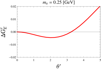
Figure 5: Relative change in the isovector electric form factor due to twisted boundary conditions in the rest frame. Plotted versus the twisting angle $\theta^{\prime}$ is ${\Delta}G_{E}^{v}(\bm{Q}^{2},L)$ given in Eq. (69). The lattice size $L$ is fixed at $2.75\,\texttt{fm}$, and the momentum transfer is $|\bm{Q}|=\theta^{\prime}/L=\theta^{\prime}\times 0.072\,\texttt{GeV}$.

Consider first the finite volume corrections to the isovector electric form factor $G_{E}^{v}(\bm{Q}^{2})$. To access this form factor, we use unpolarized matrix elements of the time component of the current. We find

$$G_{E}^{v}(\bm{Q}^{2},L)=G^{v}_{E}(\bm{Q}^{2})+{\delta}_{L}[G_{E}^{v}(\bm{Q}^{2})],$$ (68)

where $G_{E}^{v}(\bm{Q}^{2})$ is the infinite volume form factor given by Eq. (LABEL:eq:GEv), and ${\delta}_{L}[G_{E}^{v}(\bm{Q}^{2})]$ is the finite volume correction which is identical to the unpolarized matrix element in Eq. (LABEL:eq:GEvRest). Here we work with the momentum transfer entirely due to twisting $\bm{Q}=\bm{B}^{\prime}=\bm{\theta^{\prime}}/L$, and take $\bm{\theta^{\prime}}$ to lie along one spatial direction. Notice the finite volume correction to the isovector electric form factor is independent of any unphysical parameters, in particular the coupling $g_{1}$. The infinite volume isovector electric form factor depends on the parameter $c_{I}(\mu)$, the value of which can be inferred from the charge radii of the proton and neutron. Using the Particle Data Group averages Amsler et al. (2008), we find $c_{I}(\mu=1\,\texttt{GeV})=-0.393$. In Figure 5, we plot the relative change in the isovector electric form factor due to volume effects ${\Delta}G^{v}_{E}$ defined by

$${\Delta}G^{v}_{E}(\bm{Q}^{2},L)=\frac{G_{E}^{v}(\bm{Q}^{2},L)-G^{v}_{E}(\bm{Q}^{2})}{G^{v}_{E}(\bm{Q}^{2})}.$$ (69)

Here we keep the box size fixed at $2.75\,\texttt{fm}$, and plot versus the twisting angle $\theta^{\prime}$. Qualitatively the finite volume effect oscillates about the infinite volume form factor as $\theta^{\prime}$ is increased. The oscillations are damped, but this behavior is apparent at momentum transfers too large to trust the effective theory. There are no finite size effects at $\theta^{\prime}=0$ because of charge non-renormalization (which holds due to treating the time direction as infinite). The results are shown for $m_{\pi}=0.25\,\texttt{GeV}$ with the finite volume effect generally at the percent level or less. The effect of finite volume is of course smaller for larger pion masses.

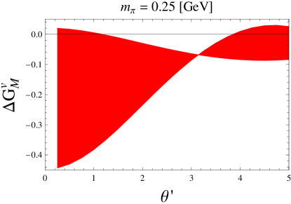
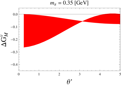
Figure 6: Relative change in the isovector magnetic form factor due to twisted boundary conditions in the rest frame. Plotted versus the twisting angle $\theta^{\prime}$ is ${\Delta}G_{M}^{v}(\bm{Q}^{2},L)$ given in Eq. (72). The lattice size $L$ is fixed at $2.75\,\texttt{fm}$, and the momentum transfer is $|\bm{Q}|=\theta^{\prime}/L=\theta^{\prime}\times 0.072\,\texttt{GeV}$. The bands arise from uncertainty in the low-energy constant $g_{1}$, which we vary assuming it is of natural size.

Considering the spatial components of the current, we can determine the magnetic form factor. Additionally there are volume corrections to the spatial current, and the net effect has the form

$$G_{M}^{v}(\bm{Q}^{2},L)=G^{v}_{M}(\bm{Q}^{2})+{\delta}_{L}[G_{M}^{v}(\bm{Q}^{2})],$$ (70)

where $G_{M}^{v}(\bm{Q}^{2})$ is the infinite volume form factor given by Eq. (59) and ${\delta}_{L}[G_{M}^{v}(\bm{Q}^{2})]$ is the finite volume correction, which follows from Eq. (LABEL:eq:GMvRest). Choosing for simplicity $\bm{B}^{\prime}=B^{\prime}\hat{\bm{y}}$, and utilizing the $\hat{\bm{z}}$ component of the current between an initial state spin-up and final state spin-down, we have

$${\delta}_{L}[G_{M}^{v}(\bm{Q}^{2})] = \frac{-2M_{N}}{B^{\prime}f^{2}}(g_{A}^{2}+g_{A}g_{1}){\mathcal{K}}^{2}(m_{\pi},B^{\prime}\bm{\hat{y}},0)$$ (71)

$$+\frac{3M_{N}}{f^{2}}\int_{0}^{1}dx\Big{[}g_{A}^{2}{\mathcal{L}}^{33}(m_{\pi}P_{\pi},\bm{0},B^{\prime}\bm{\hat{y}},xB^{\prime}\bm{\hat{y}},0)$$

$$\phantom{spacespace}+\frac{2}{9}g_{{\Delta}N}^{2}{\mathcal{L}}^{33}(m_{\pi}P_{\pi},\bm{0},B^{\prime}\bm{\hat{y}},xB^{\prime}\bm{\hat{y}},{\Delta})\Big{]}.$$

Notice this volume correction depends on the unphysical coupling $g_{1}$ which arises as a consequence of having enlarged the valence flavor group. The infinite volume isovector magnetic form factor depends upon the parameter $\mu_{I}$ which we can estimate using the known values of the proton and neutron magnetic moments. We find $\mu_{I}=6.77$. In Figure 6, we plot the relative change in the isovector magnetic form factor due to volume effects ${\Delta}G^{v}_{M}$ defined by

$${\Delta}G^{v}_{M}(\bm{Q}^{2},L)=\frac{G_{M}^{v}(\bm{Q}^{2},L)-G^{v}_{M}(\bm{Q}^{2})}{G^{v}_{M}(\bm{Q}^{2})}.$$ (72)

Again we keep the box size fixed at $2.75\,\texttt{fm}$, and plot versus the twisting angle $\theta^{\prime}$. Because the effect is non-negligible, we choose a few values of the pion mass. The result, moreover, is sensitive to the value of $g_{1}$ which has been varied assuming natural size, $-2\leq g_{1}\leq 2$. In Figure 7, we compare the extracted form factor at finite volume $G_{M}^{v}(\bm{Q}^{2},L)$ with the infinite volume form factor $G_{M}^{v}(\bm{Q}^{2})$ as a function of $\bm{Q}^{2}=\theta^{\prime}{}^{2}/L^{2}$. In this figure, we keep the lattice size at $2.75\,\texttt{fm}$, and fix the pion mass to be $0.25\,\texttt{GeV}$. Furthermore, we choose the value of $g_{1}$ favored by comparing with $SU(3)$ chiral perturbation theory, namely $g_{1}=2(F-D)\approx-0.5$.

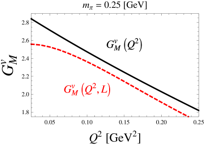
Figure 7: Comparison of finite volume and infinite volume isovector magnetic form factors. Plotted as functions of $\bm{Q}^{2}$ are the infinite volume form factor $G_{M}^{v}(\bm{Q}^{2})$, and finite volume form factor $G_{M}^{v}(\bm{Q}^{2},L)$. The lattice size is $2.75\,\texttt{fm}$, and the value of the unknown axial coupling has been fixed to $g_{1}=-0.5$.

Lastly we comment on the size of volume corrections in the Breit frame. Comparing the expressions for the isovector electric form factor in the rest frame Eq. (LABEL:eq:GEvRest), and the Breit frame Eq. (66), we see that all factors depending on $\bm{B}$ but not $\bm{Q}$ are doubled in the Breit frame. This is due to the symmetry under the exchange of the initial and final state twists: the finite volume functions are even. Because there is some cancellation among the contributions to the finite volume electric form factor in the rest frame, we can anticipate that the finite volume corrections in the Breit frame will generally be of the same size. For the magnetic form factor, comparing Eq. (LABEL:eq:GMvRest) and Eq. (67) shows similarly that the effect from the ${\mathcal{K}}^{j}$ terms doubles. While this function is odd with respect to argument, terms from the initial and final states add coherently because there is a relative sign from the spin algebra. Because empirically we observe the dominant volume correction arises from the ${\mathcal{K}}^{j}$ term, the volume effect for the magnetic form factor will roughly double in magnitude in the Breit frame. Given that the coefficient of this term depends upon the unphysical and unknown parameter $g_{1}$, the Breit frame does not offer an advantage over the rest frame. A lattice calculation of $g_{1}$ is necessary to control the systematic uncertainty from volume effects in this approach. This is not the case for isospin twisted boundary conditions Tiburzi (2006), see Appendix B.

V Summary

In this work, we compute finite volume modifications induced by partially twisted boundary conditions. We utilize heavy baryon chiral perturbation theory in finite volume. Baryons are embedded into representations of $SU(7|5)$, where the extra flavors are fictitious, and differ only in their boundary conditions. The nucleon mass splittings are determined, and demonstrated to be negligible on current-sized lattices. The main focus of our work is the derivation of finite volume corrections to the vector current matrix elements of the nucleon. Continuous momentum is inserted on the active valence quark lines using flavor changing currents in the enlarged flavor group. Disconnected operator insertions cannot be accessed at continuous momentum using this technique, and our calculation is therefore restricted to connected current insertions. Isospin breaking and cubic symmetry breaking lead to various structures not encountered in infinite volume. We give complete expressions for finite volume current matrix elements using general kinematics. To estimate the size of these corrections, we choose rest frame kinematics, and consider both the spatial and temporal components of the current. Generally the volume corrections lead to oscillatory behavior about the infinite volume answer. In the region of small twist angles, the volume effects can become rather pronounced due to terms that break cubic symmetry. To extract the isovector magnetic moment and electromagnetic radii from lattice data at zero Fourier momentum, careful determination of volume effects will be required. This is complicated by the dependence on an unphysical and unknown axial coupling $g_{1}$. As shown in Appendix B, a different implementation of twisted boundary conditions can eliminate this dependence. In this implementation, there are no fictitious flavors, rather the isospin transition is simulated directly. Compared to the meson sector, the baryon sector appears more susceptible to volume corrections due to partial twisting. The Breit frame kinematics do not simplify or reduce the volume corrections. Partial twisting provides a novel way to probe any isovector nucleon matrix element at continuous values of momentum transfer. The formalism developed here allows one to compute finite volume modifications to these observables, and thereby control the extraction of moments, radii, etc, from lattice QCD data.

Appendix A Finite Volume Current Matrix Elements

In this Appendix, we list the finite volume corrections to current matrix elements. For ease of presentation, we remove the Pauli spinors. Here we work in a general frame where the initial-state nucleon has momentum $\bm{B}=\bm{\theta}/L$, and the final-state nucleon has momentum $\bm{B}^{\prime}+\bm{q}$, where $\bm{q}$ is a Fourier momentum mode of the lattice and $\bm{B}^{\prime}=\bm{\theta^{\prime}}/L$. Here we list only the proton matrix elements as a function of $q_{u}$ and $q_{d}$. One can use charge symmetry, $q_{u}\leftrightarrow q_{d}$, to deduce the neutron matrix elements. As explained in the main text, each result includes only connected part of the matrix elements.

The finite volume modification to the time-component of the current matrix element in Eq. (36) reads

$${\delta}J_{4} = \frac{1}{f^{2}}\int_{0}^{1}dx(2q_{u}+q_{d})\left[{\mathcal{I}}_{1/2}(m_{ju}P_{ju},x\bm{Q}+\bm{B})-\frac{1}{2}{\mathcal{I}}_{1/2}(m_{ju},\bm{B})-\frac{1}{2}{\mathcal{I}}_{1/2}(m_{ju},\bm{B}^{\prime})\right]$$ (73)

$$-\frac{3}{2f^{2}}\Bigg{\{}\left(q_{d}+\frac{1}{2}q_{u}\right)\Bigg{[}g_{\pi N_{\bm{3}}N_{\bm{3}}}^{2}{\overline{{\mathcal{J}}}}(m_{\pi},\bm{0},0)+g_{juN_{\bm{3}}N_{\bm{3}}}^{2}{\overline{{\mathcal{J}}}}(m_{ju},\bm{0},0)+\frac{1}{2}g_{\pi N_{\bm{3}}N_{\bm{3}}}^{\prime\,2}\Big{(}{\overline{{\mathcal{J}}}}(m_{\pi},\bm{B},0)+{\overline{{\mathcal{J}}}}(m_{\pi},\bm{B}^{\prime},0)\Big{)}$$

$$\phantom{spaspaspa}+\frac{1}{2}g_{juN_{\bm{3}}N_{\bm{3}}}^{\prime\,2}\Big{(}{\overline{{\mathcal{J}}}}(m_{ju},\bm{B},0)+{\overline{{\mathcal{J}}}}(m_{ju},\bm{B}^{\prime},0)\Big{)}\Bigg{]}$$

$$\phantom{spa}+\frac{3}{2}q_{u}\Bigg{[}g_{\pi N_{\bm{1}}N_{\bm{1}}}^{2}{\overline{{\mathcal{J}}}}(m_{\pi},\bm{0},0)+g_{juN_{\bm{1}}N_{\bm{1}}}^{2}{\overline{{\mathcal{J}}}}(m_{ju},\bm{0},0)+\frac{1}{2}g_{\pi N_{\bm{1}}N_{\bm{1}}}^{\prime\,2}\Big{(}{\overline{{\mathcal{J}}}}(m_{\pi},\bm{B},0)+{\overline{{\mathcal{J}}}}(m_{\pi},\bm{B}^{\prime},0)\Big{)}$$

$$\phantom{spaspaspa}+\frac{1}{2}g_{juN_{\bm{1}}N_{\bm{1}}}^{\prime\,2}\Big{(}{\overline{{\mathcal{J}}}}(m_{ju},\bm{B},0)+{\overline{{\mathcal{J}}}}(m_{ju},\bm{B}^{\prime},0)\Big{)}\Bigg{]}$$

$$\phantom{spaspa}+\left(q_{d}+\frac{1}{2}q_{u}\right)\frac{g_{{\Delta}N}^{2}}{9}\Bigg{[}{\overline{{\mathcal{J}}}}(m_{\pi},\bm{0},{\Delta})+2{\overline{{\mathcal{J}}}}(m_{ju},\bm{0},{\Delta})+\frac{5}{2}\Big{(}{\overline{{\mathcal{J}}}}(m_{\pi},\bm{B},{\Delta})+{\overline{{\mathcal{J}}}}(m_{\pi},\bm{B}^{\prime},{\Delta})\Big{)}$$

$$\phantom{spaspaspa}+2\Big{(}{\overline{{\mathcal{J}}}}(m_{ju},\bm{B},{\Delta})+{\overline{{\mathcal{J}}}}(m_{ju},\bm{B}^{\prime},{\Delta})\Big{)}\Bigg{]}$$

$$\phantom{spa}+\left(\frac{3}{2}q_{u}\right)\frac{g_{{\Delta}N}^{2}}{3}\Bigg{[}{\overline{{\mathcal{J}}}}(m_{\pi},\bm{0},{\Delta})+2{\overline{{\mathcal{J}}}}(m_{ju},\bm{0},{\Delta})+\frac{1}{2}\Big{(}{\overline{{\mathcal{J}}}}(m_{\pi},\bm{B},{\Delta})+{\overline{{\mathcal{J}}}}(m_{\pi},\bm{B}^{\prime},{\Delta})\Big{)}\Bigg{]}\Bigg{\}}$$

$$+\frac{3}{2f^{2}}\Bigg{\{}\left(q_{d}+\frac{1}{2}q_{u}\right)\left[g_{\pi N_{\bm{3}}N_{\bm{3}}}^{2}{\overline{{\mathcal{J}}}}(m_{\pi},\bm{0},0)+\frac{1}{3}(g_{A}^{2}-g_{A}g_{1}-g_{1}^{2}/2)\Big{(}{\overline{{\mathcal{J}}}}(m_{\pi},\bm{B},0)+{\overline{{\mathcal{J}}}}(m_{\pi},\bm{B}^{\prime},0)\Big{)}+g_{juN_{\bm{3}}N_{\bm{3}}}^{2}{\overline{{\mathcal{J}}}}(m_{ju},\bm{0},0)\right]$$

$$\phantom{spaspaspa}+\frac{3}{2}q_{u}\left[g_{\pi N_{\bm{1}}N_{\bm{1}}}^{2}{\overline{{\mathcal{J}}}}(m_{\pi},\bm{0},0)+\frac{1}{9}(g_{A}^{2}+5g_{A}g_{1}-g_{1}^{2}/2)\Big{(}{\overline{{\mathcal{J}}}}(m_{\pi},\bm{B},0)+{\overline{{\mathcal{J}}}}(m_{\pi},\bm{B}^{\prime},0)\Big{)}+g_{juN_{\bm{1}}N_{\bm{1}}}^{2}{\overline{{\mathcal{J}}}}(m_{ju},\bm{0},0)\right]$$

$$\phantom{spaspa}+g_{{\Delta}N}^{2}\Bigg{[}\left(q_{d}+\frac{1}{2}q_{u}\right)\left(\frac{1}{9}{\overline{{\mathcal{J}}}}(m_{\pi},\bm{0},{\Delta})+\frac{1}{9}\Big{(}{\overline{{\mathcal{J}}}}(m_{\pi},\bm{B},{\Delta})+{\overline{{\mathcal{J}}}}(m_{\pi},\bm{B}^{\prime},{\Delta})\Big{)}+\frac{2}{9}{\overline{{\mathcal{J}}}}(m_{ju},\bm{0},{\Delta})\right)$$

$$\phantom{spaspaspa}+\frac{3}{2}q_{u}\left(\frac{1}{3}{\overline{{\mathcal{J}}}}(m_{\pi},\bm{0},{\Delta})+\frac{1}{3}\Big{(}{\overline{{\mathcal{J}}}}(m_{\pi},\bm{B},{\Delta})+{\overline{{\mathcal{J}}}}(m_{\pi},\bm{B}^{\prime},{\Delta})\Big{)}+\frac{2}{3}{\overline{{\mathcal{J}}}}(m_{ju},\bm{0},{\Delta})\right)\Bigg{]}\Bigg{\}}$$

$$-\frac{3}{f^{2}}[\bm{S}\cdot\bm{Q},S_{j}]\int_{0}^{1}dx\left[{\beta}_{\pi}{\mathcal{J}}^{j}(m_{\pi}P_{\pi},\bm{B},x\bm{Q}+\bm{B},0)+{\beta}_{ju}{\mathcal{J}}^{j}(m_{ju}P_{ju},\bm{B},x\bm{Q}+\bm{B},0)\right]$$

$$-\frac{3g_{{\Delta}N}^{2}}{f^{2}}[\bm{S}\cdot\bm{Q},S_{j}]\int_{0}^{1}dx\left[{\beta}^{\prime}_{\pi}{\mathcal{J}}^{j}(m_{\pi}P_{\pi},\bm{B},x\bm{Q}+\bm{B},{\Delta})+{\beta}^{\prime}_{ju}{\mathcal{J}}^{j}(m_{ju}P_{ju},\bm{B},x\bm{Q}+\bm{B},{\Delta})\right]$$

$$-\frac{3}{2f^{2}}\int_{0}^{1}dx\left[{\beta}_{\pi}{\mathcal{J}}(m_{\pi}P_{\pi},\bm{B},\bm{Q}+\bm{B},x\bm{Q}+\bm{B},0)+{\beta}_{ju}{\mathcal{J}}(m_{ju}P_{ju},\bm{B},\bm{Q}+\bm{B},x\bm{Q}+\bm{B},0)\right]$$

$$+\frac{3g_{{\Delta}N}^{2}}{f^{2}}\int_{0}^{1}dx\left[{\beta}_{\pi}^{\prime}{\mathcal{J}}(m_{\pi}P_{\pi},\bm{B},\bm{Q}+\bm{B},x\bm{Q}+\bm{B},{\Delta})+{\beta}_{ju}^{\prime}{\mathcal{J}}(m_{ju}P_{ju},\bm{B},\bm{Q}+\bm{B},x\bm{Q}+\bm{B},{\Delta})\right].$$

The effective axial couplings have been given above in Eqs. (21) and (23), while the loop coefficients appear in Eqs. (44) and (45). The spatial components of the current matrix element in Eq. (36) receive the finite volume modification

$${\delta}J_{i} = -\frac{1}{2f^{2}}\Bigg{\{}\left(q_{d}+\frac{1}{2}q_{u}\right)\Big{[}g^{\prime\,2}_{\pi N_{\bm{3}}N_{\bm{3}}}\Big{(}{\mathcal{K}}^{i}(m_{\pi},\bm{B},0)+{\mathcal{K}}^{i}(m_{\pi},\bm{B}^{\prime},0)\Big{)}+g^{\prime\,2}_{juN_{\bm{3}}N_{\bm{3}}}\Big{(}{\mathcal{K}}^{i}(m_{ju},\bm{B},0)+{\mathcal{K}}^{i}(m_{ju},\bm{B}^{\prime},0)\Big{)}\Big{]}$$ (74)

$$\phantom{space}+\frac{3}{2}q_{u}\Big{[}g^{\prime\,2}_{\pi N_{\bm{1}}N_{\bm{1}}}\Big{(}{\mathcal{K}}^{i}(m_{\pi},\bm{B},0)+{\mathcal{K}}^{i}(m_{\pi},\bm{B}^{\prime},0)\Big{)}+g^{\prime\,2}_{juN_{\bm{1}}N_{\bm{1}}}\Big{(}{\mathcal{K}}^{i}(m_{ju},\bm{B},0)+{\mathcal{K}}^{i}(m_{ju},\bm{B}^{\prime},0)\Big{)}\Big{]}\Bigg{\}}$$

$$-\frac{[S_{i},S_{j}]}{f^{2}}\Bigg{\{}\left(q_{d}+\frac{1}{2}q_{u}\right)\Big{[}g^{\prime\,2}_{\pi N_{\bm{3}}N_{\bm{3}}}\Big{(}{\mathcal{K}}^{j}(m_{\pi},\bm{B},0)-{\mathcal{K}}^{j}(m_{\pi},\bm{B}^{\prime},0)\Big{)}+g^{\prime\,2}_{juN_{\bm{3}}N_{\bm{3}}}\Big{(}{\mathcal{K}}^{j}(m_{ju},\bm{B},0)-{\mathcal{K}}^{j}(m_{ju},\bm{B}^{\prime},0)\Big{)}\Big{]}$$

$$\phantom{space}+\frac{3}{2}q_{u}\Big{[}g^{\prime\,2}_{\pi N_{\bm{1}}N_{\bm{1}}}\Big{(}{\mathcal{K}}^{j}(m_{\pi},\bm{B},0)-{\mathcal{K}}^{j}(m_{\pi},\bm{B}^{\prime},0)\Big{)}+g^{\prime\,2}_{juN_{\bm{1}}N_{\bm{1}}}\Big{(}{\mathcal{K}}^{j}(m_{ju},\bm{B},0)-{\mathcal{K}}^{j}(m_{ju},\bm{B}^{\prime},0)\Big{)}\Big{]}\Bigg{\}}$$

$$-\frac{g_{{\Delta}N}^{2}}{3f^{2}}\Bigg{\{}\left(q_{d}+\frac{1}{2}q_{u}\right)\Big{[}\frac{5}{6}\Big{(}{\mathcal{K}}^{i}(m_{\pi},\bm{B},{\Delta})+{\mathcal{K}}^{i}(m_{\pi},\bm{B}^{\prime},{\Delta})\Big{)}+\frac{2}{3}\Big{(}{\mathcal{K}}^{i}(m_{ju},\bm{B},{\Delta})+{\mathcal{K}}^{i}(m_{ju},\bm{B}^{\prime},{\Delta})\Big{)}\Big{]}$$

$$\phantom{space}+\left(\frac{3}{2}q_{u}\right)\frac{1}{2}\Big{(}{\mathcal{K}}^{i}(m_{\pi},\bm{B},{\Delta})+{\mathcal{K}}^{i}(m_{\pi},\bm{B}^{\prime},{\Delta})\Big{)}\Bigg{\}}$$

$$+g_{{\Delta}N}^{2}\frac{[S_{i},S_{j}]}{3f^{2}}\Bigg{\{}\left(q_{d}+\frac{1}{2}q_{u}\right)\Big{[}\frac{5}{6}\Big{(}{\mathcal{K}}^{j}(m_{\pi},\bm{B},{\Delta})-{\mathcal{K}}^{j}(m_{\pi},\bm{B}^{\prime},{\Delta})\Big{)}+\frac{2}{3}\Big{(}{\mathcal{K}}^{j}(m_{ju},\bm{B},{\Delta})-{\mathcal{K}}^{j}(m_{ju},\bm{B}^{\prime},{\Delta})\Big{)}\Big{]}$$

$$\phantom{space}+\left(\frac{3}{2}q_{u}\right)\frac{1}{2}\Big{(}{\mathcal{K}}^{j}(m_{\pi},\bm{B},{\Delta})-{\mathcal{K}}^{j}(m_{\pi},\bm{B}^{\prime},{\Delta})\Big{)}\Bigg{\}}$$

$$-\frac{3}{4f^{2}}\int_{0}^{1}dx\left[{\beta}_{\pi}{\mathcal{L}}^{i}(m_{\pi}P_{\pi},\bm{B},\bm{Q}+\bm{B},x\bm{Q}+\bm{B},0)+{\beta}_{ju}{\mathcal{L}}^{i}(m_{ju}P_{ju},\bm{B},\bm{Q}+\bm{B},x\bm{Q}+\bm{B},0)\right]$$

$$+\frac{3g_{{\Delta}N}^{2}}{2f^{2}}\int_{0}^{1}dx\left[{\beta}^{\prime}_{\pi}{\mathcal{L}}^{i}(m_{\pi}P_{\pi},\bm{B},\bm{Q}+\bm{B},x\bm{Q}+\bm{B},{\Delta})+{\beta}^{\prime}_{ju}{\mathcal{L}}^{i}(m_{ju}P_{ju},\bm{B},\bm{Q}+\bm{B},x\bm{Q}+\bm{B},{\Delta})\right]$$

$$-\frac{3}{2f^{2}}[\bm{Q}\cdot\bm{S},S_{j}]\int_{0}^{1}dx\left[\beta_{\pi}{\mathcal{L}}^{ji}(m_{\pi}P_{\pi},\bm{B},\bm{Q}+\bm{B},x\bm{Q}+\bm{B},0)+\beta_{ju}{\mathcal{L}}^{ji}(m_{ju}P_{ju},\bm{B},\bm{Q}+\bm{B},x\bm{Q}+\bm{B},0)\right]$$

$$-\frac{3g_{{\Delta}N}^{2}}{2f^{2}}[\bm{Q}\cdot\bm{S},S_{j}]\int_{0}^{1}dx\left[\beta^{\prime}_{\pi}{\mathcal{L}}^{ji}(m_{\pi}P_{\pi},\bm{B},\bm{Q}+\bm{B},x\bm{Q}+\bm{B},{\Delta})+\beta^{\prime}_{ju}{\mathcal{L}}^{ji}(m_{ju}P_{ju},\bm{B},\bm{Q}+\bm{B},x\bm{Q}+\bm{B},{\Delta})\right].$$

Appearing in the above expressions for finite volume modifications are functions depending on the difference of finite volume mode sums and infinite volume momentum integrals. The various definitions are as follows:

$${\mathcal{I}}_{1/2}(m,\bm{A}) = \frac{1}{L^{3}}\sum_{\bm{n}}\frac{1}{[(\bm{k}+\bm{A})^{2}+m^{2}]^{1/2}}-\int\frac{d\bm{k}}{(2\pi)^{3}}\frac{1}{[\bm{k}^{2}+M^{2}]^{1/2}},$$ (75)

$${\mathcal{J}}(m,\bm{A},\bm{B},\bm{C},{\Delta})=\int_{0}^{\infty}d{\lambda}\,{\lambda}\left[\frac{1}{L^{3}}\sum_{\bm{n}}\frac{(\bm{k}+\bm{A})\cdot(\bm{k}+\bm{B})}{[(\bm{k}+\bm{C})^{2}+{\beta}_{\Delta}^{2}]^{5/2}}-\int\frac{d\bm{k}}{(2\pi)^{3}}\frac{(\bm{k}+\bm{A})\cdot(\bm{k}+\bm{B})}{[(\bm{k}+\bm{C})^{2}+{\beta}_{\Delta}^{2}]^{5/2}}\right],$$ (76)

$${\mathcal{J}}{}^{j}(m,\bm{A},\bm{B},{\Delta})=\int_{0}^{\infty}d{\lambda}\,{\lambda}\left[\frac{1}{L^{3}}\sum_{\bm{n}}\frac{(\bm{k}+\bm{A})^{j}}{[(\bm{k}+\bm{B})^{2}+{\beta}_{\Delta}^{2}]^{5/2}}-\int\frac{d\bm{k}}{(2\pi)^{3}}\frac{(\bm{k}+\bm{A})^{j}}{[(\bm{k}+\bm{B})^{2}+{\beta}_{\Delta}^{2}]^{5/2}}\right],$$ (77)

$${\mathcal{K}}^{j}(m,\bm{B},{\Delta})=\int_{0}^{\infty}d{\lambda}\frac{1}{L^{3}}\sum_{\bm{n}}\frac{(\bm{k}+\bm{B})^{j}}{[(\bm{k}+\bm{B})^{2}+{\beta}_{\Delta}^{2}]^{3/2}},$$ (78)

$${\mathcal{L}}^{j}(m,\bm{A},\bm{B},\bm{C},{\Delta}) = \int_{0}^{\infty}d{\lambda}\Bigg{[}\frac{1}{L^{3}}\sum_{\bm{n}}\frac{(\bm{k}+\bm{A})\cdot(\bm{k}+\bm{B})(2\bm{k}+\bm{A}+\bm{B})^{j}}{[(\bm{k}+\bm{C})^{2}+{\beta}_{\Delta}^{2}]^{5/2}}$$ (79)

$$\phantom{spacespace}-\int\frac{d\bm{k}}{(2\pi)^{3}}\frac{(\bm{k}+\bm{A})\cdot(\bm{k}+\bm{B})(2\bm{k}+\bm{A}+\bm{B})^{j}}{[(\bm{k}+\bm{C})^{2}+{\beta}_{\Delta}^{2}]^{5/2}}\Bigg{]},$$

and

$${\mathcal{L}}^{ij}(m,\bm{A},\bm{B},\bm{C},{\Delta})=\int_{0}^{\infty}d{\lambda}\left[\frac{1}{L^{3}}\sum_{\bm{n}}\frac{(\bm{k}+\bm{A})^{i}(2\bm{k}+\bm{A}+\bm{B})^{j}}{[(\bm{k}+\bm{C})^{2}+{\beta}_{\Delta}^{2}]^{5/2}}-\int\frac{d\bm{k}}{(2\pi)^{3}}\frac{(\bm{k}+\bm{A})^{i}(2\bm{k}+\bm{A}+\bm{B})^{j}}{[(\bm{k}+\bm{C})^{2}+{\beta}_{\Delta}^{2}]^{5/2}}\right].$$ (80)

We also use the short hand ${\overline{{\mathcal{J}}}}(m,\bm{A},{\Delta})\equiv{\mathcal{J}}(m,\bm{A},\bm{A},\bm{A},{\Delta})$. We show how to evaluate these functions numerically in Appendix C.

Appendix B Finite Volume Isovector Current Matrix Elements from $SU(4|2)$

In this Appendix, we detail the finite volume corrections to current matrix elements using the alternate implementation of partially twisted boundary conditions proposed in Tiburzi (2005a, 2006). This method does not rely on fictitious flavors of valence quarks. Instead, one directly confronts the isospin changing operators whose matrix elements give rise to isovector form factors. From the outset, one is aware that disconnected contributions cannot be accessed. The flavor structure, moreover, only requires a simple modification of existing partially quenched theories to include twisted boundary conditions. Results for the finite volume isovector magnetic form factor under simplifying kinematics were given in Tiburzi (2006); however, as complete expressions for finite volume current matrix elements were not presented, we give the complete expressions here.

Let us briefly summarize the setup used in Tiburzi (2006). We restrict our attention to an $SU(4|2)$ theory with quarks contained in a field $Q$, which is given by $Q=(u,d,j,l,\tilde{u},\tilde{d})^{T}$. Each quark is periodic but coupled to a uniform Abelian gauge potential $B_{\mu}$ of the form $B_{\mu}=\text{diag}(B_{\mu}^{u},B_{\mu}^{d},0,0,B_{\mu}^{u},B_{\mu}^{d})$, with $B_{\mu}^{u}=(\bm{\theta}^{u}/L,0)$ and $B_{\mu}^{d}=(\bm{\theta}^{d}/L,0)$. In this formulation, momentum is injected by isospin changing operators provided $B_{\mu}^{d}\neq B_{\mu}^{d}$. Keeping these twists different introduces isospin breaking via finite volume effects. The partially quenched isospin splittings for the pion were numerically demonstrated to be quite small on current lattices Jiang and Tiburzi (2007). To calculate the nucleon isospin splitting, we evaluate the sunset diagrams shown in Figure 1 in the partially twisted $SU(4|2)$ theory. The nucleon isospin splitting is given by

$$M_{n}-M_{p} = -\frac{1}{2f^{2}}\Bigg{\{}\frac{1}{6}g_{juNN}^{2}\big{[}{\mathcal{K}}(m_{ju},\bm{B}_{d},0)-{\mathcal{K}}(m_{ju},\bm{B}_{u},0)\big{]}$$ (81)

$$\phantom{space}-\frac{2}{9}g_{{\Delta}N}^{2}\big{[}{\mathcal{K}}(m_{ju},\bm{B}_{d},{\Delta})-{\mathcal{K}}(m_{ju},\bm{B}_{u},{\Delta})\big{]}\Bigg{\}}.$$

The effective axial coupling $g_{juNN}^{2}$ has been given in Eq. (56). When the twists are isospin symmetric, the nucleon mass splitting accordingly vanishes. The maximal isospin splitting is occurs when $\bm{B}=\pi(1,1,1)$ for one flavor, and $\bm{B}=\bm{0}$ for the other. On current lattices this maximal splitting is at the percent level and can practically be ignored.

For the operator $J^{+}_{\mu}={\overline{u}}\gamma_{\mu}d$, continuous three-momentum of the form $\bm{B}_{\pi}=\bm{B}^{u}-\bm{B}^{d}$ is induced in flavor changing matrix elements. Thus we consider the isovector-vector current matrix elements between nucleons

$$\langle p(\bm{q})|J^{+}_{\mu}|n(\bm{0})\rangle\overset{L\to\infty}{\longrightarrow}\langle p(\bm{P^{\prime}})|J^{+}_{\mu}|n(\bm{P})\rangle=\langle p(\bm{P^{\prime}})|J^{\text{em}}_{\mu}|p(\bm{P})\rangle-\langle n(\bm{P^{\prime}})|J^{\text{em}}_{\mu}|n(\bm{P})\rangle.$$ (82)

On the left, we have denoted only the Fourier momentum. On the right, the momentum of the initial-state nucleon due to twisting is $\bm{P}=\bm{B}^{u}+2\bm{B}^{d}$, while the final-state nucleon has momentum $\bm{P^{\prime}}=\bm{q}+2\bm{B}^{u}+\bm{B}^{d}$. The momentum transfer we denote by $\bm{Q}$ and is given here by $\bm{Q}=\bm{q}+\bm{B}_{\pi}$. The equality between the isovector-vector current and differences of the electromagnetic current matrix elements follows from the $SU(2)_{\text{valence}}$ symmetry subgroup of the full $SU(4|2)$ group. At finite volume, this symmetry is broken and one must address the volume corrections to the matrix element on the right-hand side. To determine these corrections, we evaluate the one-loop diagrams for the isospin transition matrix element using the partially twisted $SU(4|2)$ theory. The relevant diagrams are shown in Figures 3 and 4.

The finite volume modification to the time-component of the isovector current matrix element in Eq. (82) reads

$${\delta}J^{+}_{4} = \frac{1}{f^{2}}\int_{0}^{1}dx\left[{\mathcal{I}}_{1/2}(m_{ju}P_{ju},x\bm{Q}+\bm{B}_{d})-\frac{1}{2}{\mathcal{I}}_{1/2}(m_{ju},\bm{B}_{u})-\frac{1}{2}{\mathcal{I}}_{1/2}(m_{ju},\bm{B}_{d})\right]$$ (83)

$$-\frac{1}{8f^{2}}\Bigg{\{}g_{\pi NN}^{2}\Big{[}{\overline{{\mathcal{J}}}}(m_{\pi},\bm{0},0)+{\overline{{\mathcal{J}}}}(m_{\pi},\bm{B}_{\pi},0)\Big{]}+g_{juNN}^{2}\Big{[}{\overline{{\mathcal{J}}}}(m_{ju},\bm{B}_{u},0)+{\overline{{\mathcal{J}}}}(m_{ju},\bm{B}_{d},0)\Big{]}\Bigg{\}}$$

$$+\frac{g_{{\Delta}N}^{2}}{6f^{2}}\Big{[}3{\overline{{\mathcal{J}}}}(m_{\pi},\bm{0},{\Delta})+3{\overline{{\mathcal{J}}}}(m_{\pi},\bm{B}_{\pi},{\Delta})+{\overline{{\mathcal{J}}}}(m_{ju},\bm{B}_{u},{\Delta})+{\overline{{\mathcal{J}}}}(m_{ju},\bm{B}_{d},{\Delta})\Big{]}$$

$$+\frac{1}{2f^{2}}[\bm{Q}\cdot\bm{S},S_{j}]\int_{0}^{1}dx\left[g_{\pi NN}^{2}{\mathcal{J}}^{j}(m_{\pi}P_{\pi},\bm{0},x\bm{Q},0)+g_{juNN}^{2}{\mathcal{J}}^{j}(m_{ju}P_{ju},\bm{B}_{d},x\bm{Q}+\bm{B}_{d},0)\right]$$

$$+\frac{g_{{\Delta}N}^{2}}{f^{2}}[\bm{Q}\cdot\bm{S},S_{j}]\int_{0}^{1}dx\left[{\mathcal{J}}^{j}(m_{\pi}P_{\pi},\bm{0},x\bm{Q},{\Delta})+\frac{1}{3}{\mathcal{J}}^{j}(m_{ju}P_{ju},\bm{B}_{d},x\bm{Q}+\bm{B}_{d},{\Delta})\right]$$

$$+\frac{1}{4f^{2}}\int_{0}^{1}dx\left[g_{\pi NN}^{2}{\mathcal{J}}(m_{\pi}P_{\pi},\bm{0},\bm{Q},x\bm{Q},0)+g_{juNN}^{2}{\mathcal{J}}(m_{ju}P_{ju},\bm{B}_{d},\bm{Q}+\bm{B}_{d},x\bm{Q}+\bm{B}_{d},0)\right]$$

$$-\frac{g_{{\Delta}N}^{2}}{f^{2}}\int_{0}^{1}dx\left[{\mathcal{J}}(m_{\pi}P_{\pi},\bm{0},\bm{Q},x\bm{Q},{\Delta})+\frac{1}{3}{\mathcal{J}}(m_{ju}P_{ju},\bm{B}_{d},\bm{Q}+\bm{B}_{d},x\bm{Q}+\bm{B}_{d},{\Delta})\right].$$

We have omitted writing the Pauli spinors here and below. The effective axial couplings, $g_{\pi NN}^{2}$ and $g_{juNN}^{2}$, have been given above, Eq. (56). The spatial components of the current matrix element in Eq. (36) receive the finite volume modification

$${\delta}J^{+}_{i} = -\frac{1}{2f^{2}}\Bigg{\{}\frac{1}{6}g_{juNN}^{2}\Big{[}{\mathcal{K}}^{i}(m_{ju},\bm{B}_{u},0)+{\mathcal{K}}^{i}(m_{ju},\bm{B}_{d},0)\Big{]}-\frac{2}{9}g_{{\Delta}N}^{2}\Big{[}{\mathcal{K}}^{i}(m_{ju},\bm{B}_{u},{\Delta})+{\mathcal{K}}^{i}(m_{ju},\bm{B}_{d},{\Delta})\Big{]}\Bigg{\}}$$

$$+\frac{[S_{i},S_{j}]}{6f^{2}}\Bigg{\{}g_{\pi NN}^{2}{\mathcal{K}}^{j}(m_{\pi},\bm{B}_{\pi},0)+g_{juNN}^{2}\Big{[}{\mathcal{K}}^{j}(m_{ju},\bm{B}_{u},0)-{\mathcal{K}}^{j}(m_{ju},\bm{B}_{d},0)\Big{]}\Bigg{\}}$$

$$+\frac{g_{{\Delta}N}^{2}\,[S_{i},S_{j}]}{3f^{2}}\Bigg{\{}{\mathcal{K}}^{j}(m_{\pi},\bm{B}_{\pi},{\Delta})+\frac{1}{3}\Big{[}{\mathcal{K}}^{j}(m_{ju},\bm{B}_{u},{\Delta})-{\mathcal{K}}^{j}(m_{ju},\bm{B}_{d},{\Delta})\Big{]}\Bigg{\}}$$

$$+\frac{1}{8f^{2}}\int_{0}^{1}dx\left[g_{\pi NN}^{2}{\mathcal{L}}^{i}(m_{\pi}P_{\pi},\bm{0},\bm{Q},x\bm{Q},0)+g_{juNN}^{2}{\mathcal{L}}^{i}(m_{ju}P_{ju},\bm{B}_{d},\bm{Q}+\bm{B}_{d},x\bm{Q}+\bm{B}_{d},0)\right]$$

$$-\frac{g_{{\Delta}N}^{2}}{2f^{2}}\int_{0}^{1}dx\left[{\mathcal{L}}^{i}(m_{\pi}P_{\pi},\bm{0},\bm{Q},x\bm{Q},{\Delta})+\frac{1}{3}{\mathcal{L}}^{i}(m_{ju}P_{ju},\bm{B}_{d},\bm{Q}+\bm{B}_{d},x\bm{Q}+\bm{B}_{d},{\Delta})\right]$$

$$+\frac{1}{4f^{2}}[\bm{Q}\cdot\bm{S},S_{j}]\int_{0}^{1}dx\left[g_{\pi NN}^{2}{\mathcal{L}}^{ji}(m_{\pi}P_{\pi},\bm{0},\bm{Q},x\bm{Q},0)+g_{juNN}^{2}{\mathcal{L}}^{ji}(m_{ju}P_{ju},\bm{B}_{d},\bm{Q}+\bm{B}_{d},x\bm{Q}+\bm{B}_{d},0)\right]$$

$$+\frac{g_{{\Delta}N}^{2}}{2f^{2}}[\bm{Q}\cdot\bm{S},S_{j}]\int_{0}^{1}dx\left[{\mathcal{L}}^{ji}(m_{\pi}P_{\pi},\bm{0},\bm{Q},x\bm{Q},{\Delta})+\frac{1}{3}{\mathcal{L}}^{ji}(m_{ju}P_{ju},\bm{B}_{d},\bm{Q}+\bm{B}_{d},x\bm{Q}+\bm{B}_{d},{\Delta})\right].$$

From these expressions, we can simplify things by forming unpolarized (polarized) matrix elements for the temporal (spatial) part of the current. Furthermore, we restrict our attention to the unitary mass point, where $m_{ju}^{2}=m_{\pi}^{2}$, and choose the twist parameters such that $\bm{\theta}^{d}=\bm{0}$ and $\bm{\theta}^{u}=\bm{\theta}$, which corresponds to rest frame kinematics. The time component of the current becomes

$$\frac{1}{2}\sum_{m=\pm}\langle m|{\delta}J^{+}_{4}|m\rangle = \frac{1}{f^{2}}\int_{0}^{1}dx\left[{\mathcal{I}}_{1/2}(m_{\pi}P_{\pi},x\bm{Q})-\frac{1}{2}{\mathcal{I}}_{1/2}(m_{\pi},\bm{0})-\frac{1}{2}{\mathcal{I}}_{1/2}(m_{\pi},\bm{B})\right]$$ (85)

$$-\frac{3}{2f^{2}}\Bigg{\{}g_{A}^{2}\Big{[}{\overline{{\mathcal{J}}}}(m_{\pi},\bm{0},0)+{\overline{{\mathcal{J}}}}(m_{\pi},\bm{B},0)\Big{]}-\frac{4}{9}g_{{\Delta}N}^{2}\Big{[}{\overline{{\mathcal{J}}}}(m_{\pi},\bm{0},{\Delta})+{\overline{{\mathcal{J}}}}(m_{\pi},\bm{B},{\Delta})\Big{]}\Bigg{\}}$$

$$+\frac{3}{f^{2}}\int_{0}^{1}dx\Bigg{[}g_{A}^{2}\,{\mathcal{J}}(m_{\pi}P_{\pi},\bm{0},\bm{Q},x\bm{Q},0)-\frac{4}{9}g_{{\Delta}N}^{2}\,{\mathcal{J}}(m_{\pi}P_{\pi},\bm{0},\bm{Q},x\bm{Q},{\Delta})\Bigg{]},$$

with $\bm{Q}=\bm{q}+\bm{B}$. The spatial current reads

$$\langle\pm|{\delta}J^{+}_{i}|\mp\rangle = \frac{1}{f^{2}}\langle\pm|\,[S_{k},S_{j}]\,|\mp\rangle\Bigg{\{}2\delta_{ki}\left[g_{A}^{2}\,{\mathcal{K}}^{j}(m_{\pi},\bm{B},0)+\frac{2}{9}g_{{\Delta}N}^{2}\,{\mathcal{K}}^{j}(m_{\pi},\bm{B},{\Delta})\right]$$ (86)

$$+3\bm{Q}_{k}\int_{0}^{1}dx\left[g_{A}^{2}\,{\mathcal{L}}^{ji}(m_{\pi}P_{\pi},\bm{0},\bm{Q},x\bm{Q},0)+\frac{2}{9}g_{{\Delta}N}^{2}\,{\mathcal{L}}^{ji}(m_{\pi}P_{\pi},\bm{0},\bm{Q},x\bm{Q},{\Delta})\right]\Bigg{\}}.$$

We have chosen spin flip matrix elements; these are simply related to differences of spin polarized matrix elements. Because the the finite volume modifications proportional to ${\mathcal{K}}^{j}$ are non-vanishing only in the directions with non-vanishing twist, the spin and momentum transfer structure of these terms are identical to the magnetic part of the current matrix element. Consequently one cannot be sensitive to the magnetic form factor without additionally acquiring finite volume modifications from ${\mathcal{K}}^{j}$ terms. These terms are seen to be numerically larger than ${\mathcal{L}}^{ji}$, especially for small twists Tiburzi (2006). Finally, notice these results are independent of the unphysical parameter $g_{1}$.

Appendix C Finite Volume Sums

In this Appendix we describe the evaluation of the mode sums required for the finite volume corrections to the nucleon mass and isovector form factors above. In the main text, we have used various functions entering in the computation of loop graphs in finite volume. Here we evaluate each function systematically in terms of Jacobi elliptic functions and error functions.

The basic sums required are of the form

$${\mathcal{I}}_{{\beta}}(\bm{q},{\mathcal{M}}) = \frac{1}{L^{3}}\sum_{\bm{n}}\frac{1}{[(\bm{k}+\bm{q})^{2}+{\mathcal{M}}^{2}]^{\beta}}-\int\frac{d\bm{k}}{(2\pi)^{3}}\frac{1}{[\bm{k}^{2}+{\mathcal{M}}^{2}]^{\beta}},$$

$${\mathcal{I}}^{i}_{{\beta}}(\bm{q},{\mathcal{M}}) = \frac{1}{L^{3}}\sum_{\bm{n}}\frac{\bm{k}^{i}}{[(\bm{k}+\bm{q})^{2}+{\mathcal{M}}^{2}]^{\beta}}-\int\frac{d\bm{k}}{(2\pi)^{3}}\frac{\bm{k}^{i}}{[(\bm{k}+\bm{q})^{2}+{\mathcal{M}}^{2}]^{\beta}},$$

$${\mathcal{I}}^{ij}_{{\beta}}(\bm{q},{\mathcal{M}}) = \frac{1}{L^{3}}\sum_{\bm{n}}\frac{\bm{k}^{i}\bm{k}^{j}}{[(\bm{k}+\bm{q})^{2}+{\mathcal{M}}^{2}]^{\beta}}-\int\frac{d\bm{k}}{(2\pi)^{3}}\frac{\bm{k}^{i}\bm{k}^{j}}{[(\bm{k}+\bm{q})^{2}+{\mathcal{M}}^{2}]^{\beta}}.$$ (87)

The latter two functions can be derived from the first via differentiation, explicitly the relations are

$${\mathcal{I}}_{\beta}^{i}(\bm{q},{\mathcal{M}})=-\frac{1}{2({\beta}-1)}\frac{d}{d\bm{q}^{i}}{\mathcal{I}}_{{\beta}-1}(\bm{q},{\mathcal{M}})-\bm{q}^{i}{\mathcal{I}}_{\beta}(\bm{q},{\mathcal{M}}),$$ (88)

and

$${\mathcal{I}}_{\beta}^{ij}(\bm{q},{\mathcal{M}}) = \frac{1}{4({\beta}-1)({\beta}-2)}\frac{d^{2}}{d\bm{q}^{i}d\bm{q}^{j}}{\mathcal{I}}_{{\beta}-2}(\bm{q},{\mathcal{M}})$$ (89)

$$+\frac{1}{2({\beta}-1)}\left({\delta}^{ij}+\bm{q}^{i}\frac{d}{d\bm{q}^{j}}+\bm{q}^{j}\frac{d}{d\bm{q}^{i}}\right){\mathcal{I}}_{{\beta}-1}(\bm{q},{\mathcal{M}})+\bm{q}^{i}\bm{q}^{j}{\mathcal{I}}_{\beta}(\bm{q},{\mathcal{M}}).$$

Evaluating the first function in Eq. (87) for arbitrary ${\beta}$, we find

$${\mathcal{I}}_{\beta}(\bm{q},{\mathcal{M}})=\frac{1}{8\pi^{3/2}\Gamma({\beta})}\int_{0}^{\infty}d\tau\,\tau^{{\beta}-\frac{5}{2}}e^{-\tau{\mathcal{M}}^{2}}\left[\prod_{j=1}^{3}\vartheta_{3}\left(\bm{q}_{j}L/2,e^{-\frac{L^{2}}{4\tau}}\right)-1\right],$$ (90)

where $\vartheta_{3}(q,z)$ is a Jacobi elliptic function.

In the main text, we utilized several different mode sums in the evaluation of finite volume effects. We now write them out in terms of the basic finite volume functions ${\mathcal{I}}_{\beta}(\bm{q},{\mathcal{M}})$, ${\mathcal{I}}^{i}_{\beta}(\bm{q},{\mathcal{M}})$, and ${\mathcal{I}}^{ij}_{\beta}(\bm{q},{\mathcal{M}})$. With the abbreviation ${\beta}_{\Delta}^{2}=m^{2}+2{\lambda}{\Delta}+{\lambda}^{2}$, specifically we have

$${\mathcal{J}}(m,\bm{A},\bm{B},\bm{C},{\Delta}) = \int_{0}^{\infty}d{\lambda}\,{\lambda}\left[\delta^{ij}{\mathcal{I}}^{ij}_{5/2}(\bm{C},{\beta}_{\Delta})+(\bm{A}+\bm{B})^{i}{\mathcal{I}}^{i}_{5/2}(\bm{C},{\beta}_{\Delta})+\bm{A}\cdot\bm{B}\,{\mathcal{I}}_{5/2}(\bm{C},{\beta}_{\Delta})\right],$$

$${\mathcal{J}}^{j}(m,\bm{A},\bm{B},{\Delta}) = \int_{0}^{\infty}d{\lambda}\,{\lambda}\left[{\mathcal{I}}^{j}_{5/2}(\bm{B},{\beta}_{\Delta})+\bm{A}^{j}{\mathcal{I}}_{5/2}(\bm{B},{\beta}_{\Delta})\right],$$ (92)

$${\mathcal{K}}(m,\bm{A},{\Delta}) = \int_{0}^{\infty}d{\lambda}\left[\delta^{ij}{\mathcal{I}}^{ij}_{3/2}(\bm{A},{\beta}_{\Delta})+2\bm{A}^{i}{\mathcal{I}}^{i}_{3/2}(\bm{A},{\beta}_{\Delta})+\bm{A}^{2}{\mathcal{I}}_{3/2}(\bm{A},{\beta}_{\Delta})\right],$$ (93)

$${\mathcal{K}}^{j}(m,\bm{A},{\Delta}) = \int_{0}^{\infty}d{\lambda}\left[{\mathcal{I}}^{j}_{3/2}(\bm{A},{\beta}_{\Delta})+\bm{A}^{j}{\mathcal{I}}_{3/2}(\bm{A},{\beta}_{\Delta})\right],$$ (94)

$${\mathcal{L}}^{ij}(m,\bm{A},\bm{B},\bm{C},{\Delta}) = \int_{0}^{\infty}d{\lambda}\Big{[}2{\mathcal{I}}^{ij}_{5/2}(\bm{C},{\beta}_{\Delta})+2\bm{A}^{i}{\mathcal{I}}^{j}_{5/2}(\bm{C},{\beta}_{\Delta})$$ (95)

$$\phantom{space}+(\bm{A}+\bm{B})^{j}{\mathcal{I}}^{i}_{5/2}(\bm{C},{\beta}_{\Delta})+\bm{A}^{i}(\bm{A}+\bm{B})^{j}\,{\mathcal{I}}_{5/2}(\bm{C},{\beta}_{\Delta})\Big{]}.$$

Lastly the evaluation of the ${\lambda}$-integrals can be done in closed form. For completeness the required ${\lambda}$-parameter integrals are

$$\int_{0}^{\infty}d{\lambda}\,e^{-\tau({\lambda}^{2}+2b{\lambda}+c^{2})} = \frac{1}{2}\sqrt{\frac{\pi}{\tau}}e^{\tau(b^{2}-c^{2})}\operatorname{Erfc}(b\sqrt{\tau}),$$ (96)

$$\int_{0}^{\infty}d{\lambda}\,{\lambda}\,e^{-\tau({\lambda}^{2}+2b{\lambda}+c^{2})} = \frac{1}{2}\sqrt{\frac{\pi}{\tau}}e^{-\tau c^{2}}\left[\frac{1}{\sqrt{\pi\tau}}-be^{\tau b^{2}}\operatorname{Erfc}(b\sqrt{\tau})\right],$$ (97)

where $\operatorname{Erfc}(x)=1-\operatorname{Erf}(x)$, and $\operatorname{Erf}(x)$ is the standard error function.

References

- DeGrand and DeTar (2006) T. DeGrand and C. DeTar, Lattice Methods for QCD (World Scientific, 2006).
- Zinn-Justin (2002) J. Zinn-Justin, Int. Ser. Monogr. Phys. 113, 1 (2002).
- Bedaque (2004) P. F. Bedaque, Phys. Lett. B593, 82 (2004), eprint nucl-th/0402051.
- de Divitiis et al. (2004) G. M. de Divitiis, R. Petronzio, and N. Tantalo, Phys. Lett. B595, 408 (2004), eprint hep-lat/0405002.
- Sachrajda and Villadoro (2005) C. T. Sachrajda and G. Villadoro, Phys. Lett. B609, 73 (2005), eprint hep-lat/0411033.
- Bedaque and Chen (2005) P. F. Bedaque and J.-W. Chen, Phys. Lett. B616, 208 (2005), eprint hep-lat/0412023.
- Tiburzi (2005a) B. C. Tiburzi, Phys. Lett. B617, 40 (2005a), eprint hep-lat/0504002.
- Mehen and Tiburzi (2005) T. Mehen and B. C. Tiburzi, Phys. Rev. D72, 014501 (2005), eprint hep-lat/0505014.
- Flynn et al. (2005) J. M. Flynn, A. Juttner, and C. T. Sachrajda (UKQCD) (2005), eprint hep-lat/0506016.
- Guadagnoli et al. (2006) D. Guadagnoli, F. Mescia, and S. Simula, Phys. Rev. D73, 114504 (2006), eprint hep-lat/0512020.
- Aarts et al. (2007) G. Aarts, C. Allton, J. Foley, S. Hands, and S. Kim, Nucl. Phys. A785, 202 (2007), eprint hep-lat/0607012.
- Tiburzi (2006) B. C. Tiburzi, Phys. Lett. B641, 342 (2006), eprint hep-lat/0607019.
- Jiang and Tiburzi (2007) F. J. Jiang and B. C. Tiburzi, Phys. Lett. B645, 314 (2007), eprint hep-lat/0610103.
- Boyle et al. (2007) P. A. Boyle, J. M. Flynn, A. Juttner, C. T. Sachrajda, and J. M. Zanotti, JHEP 05, 016 (2007), eprint hep-lat/0703005.
- Simula (2007) S. Simula (ETMC), PoS LAT2007, 371 (2007), eprint 0710.0097.
- Boyle et al. (2008) P. A. Boyle et al., JHEP 07, 112 (2008), eprint 0804.3971.
- Jiang and Tiburzi (2008) F.-J. Jiang and B. C. Tiburzi, Phys. Rev. D78, 037501 (2008), eprint 0806.4371.
- Aoki et al. (2008) S. Aoki et al. (2008), eprint 0808.1428.
- Bernard and Golterman (1994) C. W. Bernard and M. F. L. Golterman, Phys. Rev. D49, 486 (1994), eprint [http://arXiv.org/abs]hep-lat/9306005.
- Sharpe (1997) S. R. Sharpe, Phys. Rev. D56, 7052 (1997), eprint [http://arXiv.org/abs]hep-lat/9707018.
- Golterman and Leung (1998) M. F. L. Golterman and K.-C. Leung, Phys. Rev. D57, 5703 (1998), eprint [http://arXiv.org/abs]hep-lat/9711033.
- Sharpe and Shoresh (2000) S. R. Sharpe and N. Shoresh, Phys. Rev. D62, 094503 (2000), eprint [http://arXiv.org/abs]hep-lat/0006017.
- Sharpe and Shoresh (2001) S. R. Sharpe and N. Shoresh, Phys. Rev. D64, 114510 (2001), eprint [http://arXiv.org/abs]hep-lat/0108003.
- Labrenz and Sharpe (1996) J. N. Labrenz and S. R. Sharpe, Phys. Rev. D54, 4595 (1996), eprint [http://arXiv.org/abs]hep-lat/9605034.
- Savage (2002) M. J. Savage, Nucl. Phys. A700, 359 (2002), eprint nucl-th/0107038.
- Chen and Savage (2002) J.-W. Chen and M. J. Savage, Phys. Rev. D65, 094001 (2002), eprint [http://arXiv.org/abs]hep-lat/0111050.
- Beane and Savage (2002) S. R. Beane and M. J. Savage, Nucl. Phys. A709, 319 (2002), eprint hep-lat/0203003.
- Tiburzi (2005b) B. C. Tiburzi, Phys. Rev. D72, 094501 (2005b), eprint hep-lat/0508019.
- Tiburzi and Walker-Loud (2006) B. C. Tiburzi and A. Walker-Loud, Nucl. Phys. A764, 274 (2006), eprint hep-lat/0501018.
- Gasser and Leutwyler (1987) J. Gasser and H. Leutwyler, Phys. Lett. B188, 477 (1987).
- Leutwyler (1987) H. Leutwyler, Phys. Lett. B189, 197 (1987).
- Gasser and Leutwyler (1988) J. Gasser and H. Leutwyler, Nucl. Phys. B307, 763 (1988).
- Beane (2004) S. R. Beane, Phys. Rev. D70, 034507 (2004), eprint hep-lat/0403015.
- Golterman and Pallante (2001) M. Golterman and E. Pallante, JHEP 10, 037 (2001), eprint hep-lat/0108010.
- Tiburzi (2005c) B. C. Tiburzi, Phys. Rev. D71, 054504 (2005c), eprint hep-lat/0412025.
- Arndt and Tiburzi (2003) D. Arndt and B. C. Tiburzi, Phys. Rev. D68, 094501 (2003), eprint hep-lat/0307003.
- Bernard et al. (1992) V. Bernard, N. Kaiser, J. Kambor, and U. G. Meissner, Nucl. Phys. B388, 315 (1992).
- Bernard et al. (1998) V. Bernard, H. W. Fearing, T. R. Hemmert, and U. G. Meissner, Nucl. Phys. A635, 121 (1998), eprint hep-ph/9801297.
- Tiburzi (2008) B. C. Tiburzi, Phys. Rev. D77, 014510 (2008), eprint 0710.3577.
- Amsler et al. (2008) C. Amsler et al. (Particle Data Group), Phys. Lett. B667, 1 (2008).
- Lin and Orginos (2007) H.-W. Lin and K. Orginos (2007), eprint 0712.1214.