Comment on: “On the characteristic polynomial of an effective Hamiltonian”

Abstract

We show that a method proposed recently, based on the characteristic polynomial of an effective Hamiltonian, had been developed several years earlier by other authors in a clearer and more general way. We outline both implementations of the approach and compare them by means of the calculation of the exceptional point closest to origin for a toy model.

In a recent paper published in this journal Zheng[1] proposed a method for improving the convergence properties of the perturbation series. The approach is based on the characteristic polynomial of an effective Hamiltonian that should not be obtained explicitly. In principle, the method is restricted to a finite vector space that can be separated into a $P$-space and a $Q$-space and one should focus on the former. Zheng applied the method to a trivial problem posed by a tridiagonal matrix of dimension $3$.

Apparently, Zheng was unaware that the same approach was put forward several years earlier by Fried and Ezra[2] with somewhat similar arguments. These authors were interested in nearly resonant molecular vibrations and applied the approach to the Barbanis Hamiltonian. The resummation method of Fried and Ezra, based on the reconstruction of the effective secular equation, is identical to Zheng’s one although the former was introduced in a more general way which does not require that the state space be finite.

In what follows we outline and compare the methods proposed by Zheng[1] and Fried and Ezra[2].

Zheng’s method[1] applies to a quantum-mechanical model defined on a state space of dimension $\tilde{N}=N+M$ spanned by an orthonormal basis set $B=\left\{\psi_{i}^{P},\;i=1,2,\ldots,N,\;\psi_{j}^{Q},\;j=1,2,\ldots,M\right\}$, where $\left\{\psi_{i}^{P}\right\}$ and $\left\{\psi_{j}^{Q}\right\}$ span the so-called $P$ and $Q$ subspaces, respectively. The approach is based on the secular determinant

$$\left|E\mathbf{I}_{\tilde{N}}-\mathbf{H}(\lambda)\right|=E^{\tilde{N}}+\sum_{j=1}^{\tilde{N}}p_{j}(\lambda)E^{\tilde{N}-j},$$ (1)

where $\mathbf{H}(\lambda)$ is the matrix representation of the Hamiltonian operator $H=H_{0}+\lambda H_{I}$ in the basis set $B$ and $\mathbf{I}_{\tilde{N}}$ is the identity matrix of dimension $\tilde{N}$. The operators $H_{0}$ and $H_{I}$ are the diagonal and off-diagonal parts of $H$ in the basis set $B$. It is clear that $p_{j}(\lambda)$ are polynomial functions of $\lambda$.

Zheng[1] took into account that

$$\left|E\mathbf{I}_{\tilde{N}}-\mathbf{H}(\lambda)\right|=\prod_{i=1}^{N}\left[E-E_{i}^{P}(\lambda)\right]\prod_{j=1}^{M}\left[E-E_{j}^{Q}(\lambda)\right],$$ (2)

where $E_{i}^{P}(\lambda)$ and $E_{j}^{Q}(\lambda)$ are determined by the conditions $E_{i}^{P}(\lambda=0)=\left\langle\psi_{i}^{P}\right|H\left|\psi_{i}^{P}\right\rangle$ and $E_{j}^{Q}(\lambda=0)=\left\langle\psi_{j}^{Q}\right|H\left|\psi_{j}^{Q}\right\rangle$ . It is worth noting that any eigenfunction $\psi_{k}$ of $H$ is a linear combination of both $\psi_{i}^{P}$ and $\psi_{j}^{Q}$ because $\left\langle\psi_{i}^{P}\right|H_{I}\left|\psi_{j}^{Q}\right\rangle\neq 0$.

Zheng’s approach is based on the equation

$$\left|E\mathbf{I}_{N}-\mathbf{H}_{\mathrm{eff}}(\lambda)\right|=\prod_{i=1}^{N}\left[E-E_{i}^{P}(\lambda)\right],$$ (3)

where each $E_{i}^{P}(\lambda)$ is a perturbation expansion

$$E_{i}^{P}(\lambda)=\sum_{j=1}^{K}E_{i,j}^{P}\lambda^{j}.$$ (4)

Since the calculation is based on the right-hand-side of equation (3) it is not necessary to find out the effective Hamiltonian operator $H_{\mathrm{eff}}$ explicitly.

Zheng[1] applied the approach just outlined to a simple model with $N=2$ and $M=1$ and showed that the approximate eigenvalues obtained in this way are considerably more accurate than the perturbation series used in the construction of the effective characteristic polynomial (3). However, we may raise the following question: why would anybody resort to this approach since the calculation of the exact eigenvalues as roots of the polynomial (1) is straightforward?.

As stated above, Fried an Ezra[2] put forward essentially the same method in a more general way by means of somewhat similar arguments. Suppose that we want to obtain the solutions to the Schrödinger equation $H\psi_{n}=E_{n}\psi_{n}$, $n=1,2,\ldots$, where $H=H_{0}+\lambda H_{I}$. To this end, we apply perturbation theory and obtain partial sums of the form

$$E_{n}^{[K]}=\sum_{j=0}^{K}E_{n,j}\lambda^{j}.$$ (5)

With them one reconstructs the effective secular equation

$$\left\{\prod_{n=1}^{N}\left[W-E_{n}^{[K]}(\lambda)\right]\right\}^{[K]}=W^{N}+\sum_{j=1}^{N}p_{j}(\lambda)W^{N-j},$$ (6)

where $\left\{...\right\}^{[K]}$ means that we remove any term with $\lambda^{j}$ if $j>K$. The reason is that the accuracy of the results cannot be greater than $\mathcal{O}\left(\lambda^{K}\right)$ determined by the partial sums (5)[2]. The eigenvalues $E_{n}$ used in this reconstruction are related to the so-called model space, which is finite, and we leave aside the complement space that is not necessarily so. The states in the model space are strongly coupled among themselves and weakly coupled to the states in the complement state.

Zheng[1] applied the method to the following tridiagonal matrix of dimension $\tilde{N}=3$:

$$\mathbf{H}(\lambda)=\left(\begin{array}[]{lll}2&\lambda&0\\ \lambda&1.1&\lambda\\ 0&\lambda&1\end{array}\right).$$ (7)

From the roots of the characteristic polynomial

$$cp(E,\lambda)=\left|E\mathbf{I}_{3}-\mathbf{H}\right|=E^{3}-\frac{41}{10}E^{2}+\frac{53-20\lambda^{2}}{10}E+\frac{15\lambda^{2}-11}{5},$$ (8)

we obtain three eigenvalues $E_{1}(\lambda)<E_{2}(\lambda)<E_{3}(\lambda)$ that satisfy $E_{1}(0)=1$, $E_{2}(0)=1.1$ and $E_{3}(0)=2$. We do not show the exact analytical expressions for $E_{i}(\lambda)$ because they are rather cumbersome. These eigenvalues do not cross because $H_{12}=H_{21}\neq 0$ and $H_{23}=H_{32}\neq 0$ (see[3] for a general analysis). Note that $E_{1}(0)$ and $E_{2}(0)$ are nearly degenerate, a fact that commonly leads to perturbation series with poor convergence properties (as discussed by Fried and Ezra[2] and Zheng[1]).

From the discriminant of the characteristic polynomial (8) (see[4] and references therein) we obtain the exceptional points $\lambda_{1}$, $\lambda_{1}^{*}$, $\lambda_{2}$, $\lambda_{2}^{*}$, $-\lambda_{2}$ and $-\lambda_{2}^{*}$, where $\lambda_{1}=0.05139217757i$ and $\lambda_{2}=0.2381164319+0.5028706167i$. This particular distribution of the exceptional points in the complex $\lambda$-plane is due to the fact that $cp(E,-\lambda)=cp(E,\lambda)$ and $cp(E,\lambda)^{*}=cp(E,\lambda)$ for $\lambda$ real. The eigenvalues $E_{1}$ and $E_{2}$ coalesce at $\lambda=\pm\lambda_{1}$ while $E_{2}$ and $E_{3}$ coalesce at $\lambda_{2}$ and its variants. Therefore, following the arguments put forward by Fried and Ezra[2] and Zheng[1], we apply the approach (6) for $N=2$ (that is to say: with perturbation approximations (5) for $E_{1}$ and $E_{2}$).

Since $cp(E,-\lambda)=cp(E,\lambda)$ we have perturbation expansions in terms of the variable $\lambda^{2}$. Figure 1 shows results obtained from equation (6) with perturbation expansions of order $K=6$. These results are similar to those shown by Zheng[1].

A most interesting feature of this approximation is that it enables us to estimate the exceptional point in the complex $\lambda$ plane closest to origin ($\lambda_{1}$ and $\lambda_{1}^{\ast}$ in the present case). This fact was overlooked by Fried and Ezra because the perturbation series for the eigenvalues of the Barbanis Hamiltonian are divergent (zero convergence radius). On the other hand, Zheng estimated the location of the exceptional point by means of the approach, using perturbation series of order $K=2,4,6$. In order to illustrate this fact explicitly, we apply the discriminant approach[4] to equation (6) and obtain the approximate exceptional points for increasing values of $K$. Table  1 shows that the approximate exceptional point $|\lambda_{1}|^{[K]}$ calculated in this way converges, as $K$ increases, towards the actual value of $|\lambda_{1}|$ obtained from the characteristic polynomial (8). Zheng’s result for $K=2$ appears to be incorrect because it agrees with the result for $K=6$ and disagrees with present one. The agreement of present results with those of Zheng for $K=4,6$ clearly reveal that the methods of Fried and Ezra and Zheng are identical; the discrepancy for $K=2$ being, most probably, due to a misprint in Zheng’s paper.

Summarizing: the aim of this Comment is to point out that Zheng[1] did not develop a new method because it was put forward several years earlier by Fried and Ezra[2]. Besides, the latter authors presented their approach in a clearer and more general way. In addition to it Fried and Ezra applied the reconstruction of the effective secular equation to more demanding quantum-mechanical models. As a by-product we verify that the method is suitable for estimating the locations of the exceptional points that determine the radius of convergence of the perturbation series used in the reconstruction of the effective secular equation.

Table 1: Convergence of the estimated exceptional point $|\lambda_{1}^{[K]}|$

$K$	Present	Zheng[1]
2	0.05147186257	0.0513922
4	0.05139244862	0.0513924
6	0.05139217790	0.0513922
8	0.05139217757
10	0.05139217757

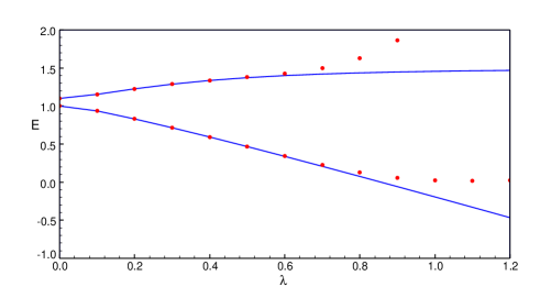
Figure 1: First two eigenvalues $E_{1}(\lambda)$ and $E_{2}(\lambda)$ calculated exactly (blue, continuous line) and by means of the approach (6) based on sixth-order perturbation theory

References

- [1] Y. Zheng, Phys. Lett. A 443 (2022) 128215.
- [2] L. E. Fried and G. S. Ezra, J. Chem. Phys. 90 (1989) 6378-6390.
- [3] F. M. Fernández, J. Math. Chem. 52 (2014) 2322.
- [4] P. Amore and F. M. Fernández, Eur. Phys. J. Plus 136 (2021) 133.