Asynchronous Actor-Critic for Multi-Agent Reinforcement Learning

Abstract

Synchronizing decisions across multiple agents in realistic settings is problematic since it requires agents to wait for other agents to terminate and communicate about termination reliably. Ideally, agents should learn and execute asynchronously instead. Such asynchronous methods also allow temporally extended actions that can take different amounts of time based on the situation and action executed. Unfortunately, current policy gradient methods are not applicable in asynchronous settings, as they assume that agents synchronously reason about action selection at every time step. To allow asynchronous learning and decision-making, we formulate a set of asynchronous multi-agent actor-critic methods that allow agents to directly optimize asynchronous policies in three standard training paradigms: decentralized learning, centralized learning, and centralized training for decentralized execution. Empirical results (in simulation and hardware) in a variety of realistic domains demonstrate the superiority of our approaches in large multi-agent problems and validate the effectiveness of our algorithms for learning high-quality and asynchronous solutions.

1 Introduction

In recent years, multi-agent policy gradient methods using the actor-critic framework have achieved impressive success in solving a variety of cooperative and competitive domains (Baker et al., 2020; Du et al., 2019; Foerster et al., 2018; Du et al., 2021; Iqbal and Sha, 2019; Li et al., 2019; Lowe et al., 2017; Su et al., 2021; Vinyals et al., 2019; Wang et al., 2020a, 2021a; Yang et al., 2020a; Zhou et al., 2020). However, as these methods assume synchronized primitive-action execution over agents, they struggle to solve large-scale real-world multi-agent problems that involve long-term reasoning and asynchronous behavior.

Temporally-extended actions have been widely used in both learning and planning to improve scalability and reduce complexity. For example, they have come in the form of motion primitives (Dalal et al., 2021; Stulp and Schaal, 2011), skills (Konidaris et al., 2011, 2018), spatial action maps (Wu et al., 2020) or macro-actions (He et al., 2010; Hsiao et al., 2010; Lee et al., 2021; Theocharous and Kaelbling, 2004). The idea of temporally-extended actions has also been incorporated into multi-agent approaches. In particular, we consider the Macro-Action Decentralized Partially Observable Markov Decision Process (MacDec-POMDP) (Amato et al., 2014, 2019). The MacDec-POMDP is a general model for cooperative multi-agent problems with partial observability and (potentially) different action durations. As a result, agents can start and end macro-actions at different time steps so decision-making can be asynchronous.

The MacDec-POMDP framework has shown strong scalability with planning-based methods (where the model is given) (Amato et al., 2015a, b; Hoang et al., 2018; Omidshafiei et al., 2016, 2017a). In terms of multi-agent reinforcement learning (MARL), there have been many hierarchical approaches, they don’t typically address asynchronicity since they assume agents’ have high-level decisions with the same duration (de Witt et al., 2019; Han et al., 2019; Nachum et al., 2019; Wang et al., 2020b, 2021b; Xu et al., 2021; Yang et al., 2020b). Only limited studies have considered asynchronicity (Chakravorty et al., 2019; Menda et al., 2019; Xiao et al., 2019), yet, none of them provides a general formulation for multi-agent policy gradients that allows agents to asynchronously learn and execute.

In this paper, we assume a set of macro-actions has been predefined for each domain. This is well-motivated by the fact that, in real-world multi-robot systems, each robot is already equipped with certain controllers (e.g., a navigation controller, and a manipulation controller) that can be modeled as macro-actions (Amato et al., 2015a; Omidshafiei et al., 2017a; Wu et al., 2021a; Xiao et al., 2019). Similarly, as it is common to assume primitive actions are given in a typical RL domain, we assume the macro-actions are given in our case. The focus of the policy gradient methods is then on learning high-level policies over macro-actions.

Our contributions include a set of macro-action-based multi-agent actor-critic methods that generalize their primitive-action counterparts. First, we formulate a macro-action-based independent actor-critic (Mac-IAC) method. Although independent learning suffers from a theoretical curse of environmental non-stationarity, it allows fully online learning and may still work well in certain domains. Second, we introduce a macro-action-based centralized actor-critic (Mac-CAC) method, for the case where full communication is available during execution. We also formulate a centralized training for decentralized execution (CTDE) paradigm (Kraemer and Banerjee, 2016; Oliehoek et al., 2008) variant of our method. CTDE has gained popularity since such methods can learn better decentralized policies by using centralized information during training. Current primitive-action-based multi-agent actor-critic methods typically use a centralized critic to optimize each decentralized actor. However, the asynchronous joint macro-action execution from the centralized perspective could be very different with the completion time being very different from each agent’s decentralized perspective. To this end, we first present a Naive Independent Actor with Centralized Critic (Naive IACC) method that naively uses a joint macro-action-value function as the critic for each actor’s policy gradient estimation; and then propose a novel Independent Actor with Individual Centralized Critic (Mac-IAICC) method that learns individual critics using centralized information to address the above challenge.

We evaluate our proposed methods on diverse macro-action-based multi-agent problems: a benchmark Box Pushing domain (Xiao et al., 2019), a variant of the Overcooked domain (Wu et al., 2021b) and a larger warehouse service domain (Xiao et al., 2019). Experimental results show that our methods are able to learn high-quality solutions while primitive-action-based methods cannot, and show the strength of Mac-IAICC for learning decentralized policies over Naive IAICC and Mac-IAC. Decentralized policies learned by using Mac-IAICC are successfully deployed on real robots to solve a warehouse tool delivery task in an efficient way. To our knowledge, this is the first general formalization of macro-action-based multi-agent actor-critic frameworks for the three state-of-the-art multi-agent training paradigms.

2 Background

2.1 MacDec-POMDPs

The macro-action decentralized partially observable Markov decision process (MacDec-POMDP) (Amato et al., 2014, 2019) incorporates the option framework (Sutton et al., 1999) into the Dec-POMDP by defining a set of macro-actions for each agent. Formally, a MacDec-POMDP is defined by a tuple $\langle I,S,A,M,\Omega,\zeta,T,R,O,Z,\mathbb{H},\gamma\rangle$, where $I$ is a set of agents; $S$ is the environmental state space; $A=\times_{i\in I}A_{i}$ is the joint primitive-action space over each agent’s primitive-action set $A_{i}$; $M=\times_{i\in I}M_{i}$ is the joint macro-action space over each agent’s macro-action space $M_{i}$; $\Omega=\times_{i\in I}\Omega_{i}$ is the joint primitive-observation space over each agent’s primitive-observation set $\Omega_{i}$; $\zeta=\times_{i\in I}\zeta_{i}$ is the joint macro-observation space over each agent’s macro-observation space $\zeta_{i}$; $T(s,\vec{a},s^{\prime})=P(s^{\prime}|s,\vec{a})$ is the environmental transition dynamics; and $R(s,\vec{a})$ is a global reward function. During execution, each agent independently selects a macro-action $m_{i}$ using a high-level policy $\Psi_{i}:H^{M}_{i}\times M_{i}\rightarrow[0,1]$ and captures a macro-observation $z_{i}\in\zeta_{i}$ according to the macro-observation probability function $Z_{i}(z_{i},m_{i},s^{\prime})=P(z_{i}\mid m_{i},s^{\prime})$ when the macro-action terminates in a state $s^{\prime}$. Each macro-action is represented as $m_{i}=\langle I_{m_{i}},\pi_{m_{i}},\beta_{m_{i}}\rangle$, where the initiation set $I_{m_{i}}\subset H^{M}_{i}$ defines how to initiate a macro-action based on macro-observation-action history $H^{M}_{i}$ at the high-level; $\pi_{m_{i}}:H^{A}_{i}\times A_{i}\rightarrow[0,1]$ is the low-level policy for achieving a macro-action, and during the running, the agent receives a primitive-observation $o_{i}\in\Omega_{i}$ based on the observation function $O_{i}(o_{i},a_{i},s)=P(o_{i}|a_{i},s)$ at every time step; $\beta_{m_{i}}:H^{A}_{i}\rightarrow[0,1]$ is a stochastic termination function that determines how to terminate a macro-action based on primitive-observation-action history $H^{A}_{i}$ at the low-level. The objective of solving MacDec-POMDPs with finite horizon is to find a joint high-level policy $\vec{\Psi}=\times_{i\in I}\Psi_{i}$ that maximizes the value, $V^{\vec{\Psi}}(s_{(0)})=\mathbb{E}\Big{[}\sum_{t=0}^{\mathbb{H}-1}\gamma^{t}r\big{(}s_{(t)},\vec{a}_{(t)}\big{)}\mid s_{(0)},\vec{\pi},\vec{\Psi}\Big{]}$, where $\gamma\in[0,1]$ is a discount factor, and $\mathbb{H}$ is the number of (primitive) time steps until the problem terminates (the horizon).

2.2 Single-Agent Actor-Critic

In single-agent reinforcement learning, the policy gradient theorem (Sutton et al., 2000) formulates a principled way to optimize a parameterized policy $\pi_{\theta}$ via gradient ascent on the policy’s performance defined as $J(\theta)=\mathbb{E}_{\pi_{\theta}}\big{[}\sum_{t=0}^{\infty}\gamma^{t}r\big{(}s_{(t)},a_{(t)}\big{)}\big{]}$. In POMDPs, the gradient w.r.t. parameters of a history-based policy $\pi_{\theta}(a\mid h)$ is expressed as: $\nabla_{\theta}J(\theta)=\mathbb{E}_{\pi_{\theta}}\Big{[}\nabla_{\theta}\log\pi_{\theta}(a\mid h)Q^{\pi_{\theta}}(h,a)\Big{]}$, where $h$ is maintained by a recurrent neural network (RNN) (Hausknecht and Stone, 2015). The actor-critic framework (Konda and Tsitsiklis, 2000) learns an on-policy action-value function $Q^{\pi_{\theta}}_{\phi}(h,a)$ (critic) via temporal-difference (TD) learning (Sutton, 1988) to approximate the action-value for the policy (actor) updates. Variance reduction is commonly achieved by training a history-value function $V^{\pi_{\theta}}_{\mathbf{w}}(h)$ and using it as a baseline (Weaver and Tao, 2001) as well as bootstrapping to estimate the action-value. Accordingly, the policy gradient can be written as:

$$\nabla_{\theta}J(\theta)=\mathbb{E}_{\pi_{\theta}}\Big{[}\nabla_{\theta}\log\pi_{\theta}(a\mid h)\big{(}r+\gamma V^{\pi_{\theta}}_{\mathbf{w}}(h^{\prime})-V^{\pi_{\theta}}_{\mathbf{w}}(h)\big{)}\Big{]}$$ (1)

where, $r$ is the immediate reward received by the agent at the corresponding time step.

2.3 Independent Actor-Critic

The single-agent actor-critic algorithm can be adapted to multi-agent problems in a simple way such that each agent independently learns its own actor and critic while treating other agents as part of the world (Foerster et al., 2018). We consider a variance reduction version of independent actor-critic (IAC) with the policy gradient as follows:

$$\nabla_{\theta_{i}}J(\theta_{i})=\mathbb{E}_{\vec{\pi}_{\vec{\theta}}}\Big{[}\nabla_{\theta_{i}}\log\pi_{\theta_{i}}(a_{i}|h_{i})\big{(}r+\gamma V^{\pi_{\theta_{i}}}_{\mathbf{w}_{i}}(h^{\prime}_{i})-V^{\pi_{\theta_{i}}}_{\mathbf{w}_{i}}(h_{i})\big{)}\Big{]}$$ (2)

where, $r$ is a shared reward over agents at every time step. Due to other agents’ policy updating and exploring, from any agent’s local perspective, the environment appears non-stationary which can lead to unstable learning of the critic without convergence guarantees (Lowe et al., 2017). This instability often prevents IAC from learning high-quality cooperative policies.

2.4 Independent Actor with Centralized Critic

To address the above difficulties in independent learning approaches, centralized training for decentralized execution (CTDE) provides agents with access to global information during offline training while allowing agents to rely on only local information during online decentralized execution. Typically, the key idea of exploiting CTDE with actor-critic is to train a joint action-value function, $Q^{\vec{\pi}_{\vec{\theta}}}_{\phi}(\mathbf{x},\vec{a})$, as the centralized critic and use it to compute gradients w.r.t. the parameters of each decentralized policy (Foerster et al., 2018; Lowe et al., 2017). Although the centralized critic can facilitate the update of decentralized policies to optimize global collaborative performance, it also introduces extra variance over other agents’ actions (Lyu et al., 2021; Wang et al., 2021a). Therefore, we consider the version of independent actor with centralized critic (IACC) with a general variance reduction trick (Foerster et al., 2018; Su et al., 2021), the policy gradient of which is:

$$\nabla_{\theta_{i}}J(\theta_{i})=\mathbb{E}_{\vec{\pi}_{\vec{\theta}}}\Big{[}\nabla_{\theta_{i}}\log\pi_{\theta_{i}}(a_{i}\mid h_{i})\big{(}r+\gamma V^{\vec{\pi}_{\vec{\theta}}}_{\mathbf{w}}(\mathbf{x^{\prime}})-V^{\vec{\pi}_{\vec{\theta}}}_{\mathbf{w}}(\mathbf{x})\big{)}\Big{]}$$ (3)

where, $\mathbf{x}$ represents the available centralized information (e.g., joint observation, joint observation-action history, or the true state).

2.5 Learning Macro-Action-Based Deep Q-Nets

Previous MARL methods for Dec-POMDPs cannot work with the asynchronicity of macro-action-based agents, where agents may start and complete their macro-actions at different time steps. Recently, macro-action-based multi-agent DQNs have been proposed for MacDec-POMDPs (Xiao et al., 2019).

For decentralized learning, a new buffer, Macro-Action Concurrent Experience Replay Trajectories (Mac-CERTs), is designed for collecting each agent’s macro-observation, macro-action, and reward information. In this buffer, the transition experience of each agent $i$ is represented as a tuple $\langle z_{i},m_{i},z_{i}^{\prime},r_{i}^{c}\rangle$, where $r_{i}^{c}=\sum_{t=t_{m_{i}}}^{t_{m_{i}}+\tau_{m_{i}}-1}\gamma^{t-t_{m_{i}}}r_{(t)}$ is a cumulative reward of the macro-action taking $\tau_{m_{i}}$ time steps to be completed from its beginning time step $t_{m_{i}}$. During training, a mini-batch of concurrent sequential experiences is sampled from Mac-CERTs. Each agent independently accesses its own sampled experiences and obtains ‘squeezed’ trajectories by removing the transitions in the middle of each macro-action execution, which produces a mini-batch of transitions when the corresponding macro-action terminates (i.e., removing time information). Updates for each macro-action-value function $Q_{\phi_{i}}(h_{i},m_{i})$ take place only when the agent’s macro-action is complete by minimizing a TD loss over the ‘squeezed’ data. In the centralized learning case, the objective is to learn a joint macro-action-value function $Q_{\phi}(\vec{h},\vec{m})$. To this end, another special buffer called Macro-Action Joint Experience Replay Trajectories (Mac-JERTs) is developed for collecting agents’ joint transition experience at every time step and each is represented as a tuple $\langle\vec{z},\vec{m},\vec{z\,}^{\prime},\vec{r\,}^{c}\rangle$, where $\vec{r\,}^{c}=\sum_{t=t_{\vec{m}}}^{t_{\vec{m}}+\vec{\tau}_{\vec{m}}-1}\gamma^{t-t_{\vec{m}}}r_{(t)}$ is a shared joint cumulative reward from the beginning time step $t_{\vec{m}}$ of the joint macro-action $\vec{m}$ to its termination, defined as when any agent finishes its own macro-action, after $\vec{\tau}_{\vec{m}}$ time steps. In each training iteration, the joint macro-action-value function is optimized over a mini-batch of ‘squeezed’ (depending on each joint macro-action termination) sequential joint experiences via TD learning. Other choices for what information to retain are also possible (e.g., the whole sequence of macro-actions or including time to complete) but this squeezing procedure was found to work well. In our macro-action-based actor-critic methods, we extend the above approaches to train critics on-policy, and the trajectory squeezing is changed variously for each method in order to achieve improved asynchronous macro-action-based policy updates via policy gradient.

3 Approach

MARL with asynchronous macro-actions is more challenging as it is difficult to determine when to update each agent’s policy and what information to use. Although the macro-action-based DQN methods (Xiao et al., 2019) (in Section 2.5) give us the base to learn macro-action value functions, they do not directly extend to the policy gradient case, particularly in the case of centralized training for decentralized execution (CTDE). In this section, we propose principled formulations of on-policy macro-action-based multi-agent actor-critic methods for decentralized learning (Section 3.1), centralized learning (Section 3.2), and CTDE (Section 3.3). In each case, we first introduce the version with a Q-value function as the critic and then present the variance reduction version .

3.1 Macro-Action-Based Independent Actor-Critic (Mac-IAC)

Similar to the idea of IAC with primitive-actions (Section 2.3), a straightforward extension is to have each agent independently optimize its own macro-action-based policy (actor) using a local macro-action-value function (critic). Hence, we start with deriving a macro-action-based policy gradient theorem in Appendix B by incorporating the general Bellman equation for the state values of a macro-action-based policy (Sutton et al., 1999) into the policy gradient theorem in MDPs (Sutton et al., 2000), and then extend it to MacDec-POMDPs so that each agent can have the following policy gradient w.r.t. the parameters of its macro-action-based policy $\Psi_{\theta_{i}}(m_{i}|h_{i})$ as: $\nabla_{\theta_{i}}J(\theta_{i})=\mathbb{E}_{\vec{\Psi}_{\vec{\theta}}}\biggr{[}\nabla_{\theta_{i}}\log\Psi_{\theta_{i}}(m_{i}\mid h_{i})Q^{\Psi_{\theta_{i}}}_{\phi_{i}}(h_{i},m_{i})\biggr{]}$. During training, each agent accesses its own trajectories and squeezes them in the same way as the decentralized case mentioned in Section 2.5 to train the critic $Q_{\phi_{i}}^{\Psi_{\theta_{i}}}(h_{i},m_{i})$ via on-policy TD learning and perform gradient ascent to update the policy when the agent’s macro-action terminates. In our case, we train a local history value function $V^{\Psi_{\theta_{i}}}_{\mathbf{w}_{i}}(h_{i})$ as each agent’s critic and use it as a baseline to achieve variance reduction. The corresponding policy gradient is as follows:

$$\nabla_{\theta_{i}}J(\theta_{i})=\mathbb{E}_{\vec{\Psi}_{\vec{\theta}}}\biggr{[}\nabla_{\theta_{i}}\log\Psi_{\theta_{i}}(m_{i}\mid h_{i})\big{(}r^{c}_{i}+\gamma^{\tau_{m_{i}}}V^{\Psi_{\theta_{i}}}_{\mathbf{w}_{i}}(h_{i}^{\prime})-V^{\Psi_{\theta_{i}}}_{\mathbf{w}_{i}}(h_{i})\big{)}\biggr{]}$$ (4)

where, the cumulative reward $r^{c}_{i}$ is w.r.t. the execution of agent $i$’s macro-action $m_{i}$.

3.2 Macro-Action-Based Centralized Actor-Critic (Mac-CAC)

In the fully centralized learning case, we treat all agents as a single joint agent to learn a centralized actor $\Psi_{\theta}(\vec{m}\mid\vec{h})$ with a centralized critic $Q^{\Psi_{\theta}}_{\phi}(\vec{h},\vec{m})$, and the policy gradient can be expressed as: $\nabla_{\theta}J(\theta)=\mathbb{E}_{\Psi_{\theta}}\biggr{[}\nabla_{\theta}\log\Psi_{\theta}(\vec{m}\mid\vec{h})Q^{\Psi_{\theta}}_{\phi}(\vec{h},\vec{m})\biggr{]}$. Similarly, to achieve a lower variance optimization for the actor, we learn a centralized history value function $V^{\Psi_{\theta}}_{\mathbf{w}}(\vec{h})$ by minimizing a TD-error loss over joint trajectories that are squeezed w.r.t. each joint macro-action termination (when any agent terminates its macro-action, defined in the centralized case in Section 2.5). Accordingly, the policy’s updates are performed when each joint macro-action is completed by ascending the following gradient:

$$\nabla_{\theta}J(\theta)=\mathbb{E}_{\Psi_{\theta}}\biggr{[}\nabla_{\theta}\log\Psi_{\theta}(\vec{m}\mid\vec{h})\big{(}\vec{r\,}^{c}+\gamma^{\vec{\tau}_{\vec{m}}}V^{\Psi_{\theta}}_{\mathbf{w}}(\vec{h}^{\prime})-V^{\Psi_{\theta}}_{\mathbf{w}}(\vec{h})\big{)}\biggr{]}$$ (5)

where the cumulative reward $\vec{r\,}^{c}$ is w.r.t. the execution of the joint macro-action $\vec{m}$.

3.3 Macro-Action-Based Independent Actor with Centralized Critic (Mac-IACC)

As mentioned earlier, fully centralized learning requires perfect online communication that is often hard to guarantee, and fully decentralized learning suffers from environmental non-stationarity due to agents’ changing policies. In order to learn better decentralized macro-action-based policies, in this section, we propose two macro-action-based actor-critic algorithms using the CTDE paradigm. The difference between a joint macro-action termination from the centralized perspective and a macro-action termination from each agent’s local perspective gives rise to a new challenge: what kind of centralized critic should be learned and how should it be used to optimize decentralized policies where some have completed and some have not, which we investigate below.

Naive Mac-IACC. A naive way of incorporating macro-actions into a CTDE-based actor-critic framework is to directly adapt the idea of the primitive-action-based IACC (Section 2.4) to have a shared joint macro-action-value function $Q^{\vec{\Psi}_{\vec{\theta}}}_{\phi}(\mathbf{x},\vec{m})$ in each agent’s decentralized macro-action-based policy gradient as: $\nabla_{\theta_{i}}J(\theta_{i})=\mathbb{E}_{\vec{\Psi}_{\vec{\theta}}}\biggr{[}\nabla_{\theta_{i}}\log\Psi_{\theta_{i}}(m_{i}\mid h_{i})Q^{\vec{\Psi}_{\vec{\theta}}}_{\phi}(\mathbf{x},\vec{m})\biggr{]}$. To reduce variance, with a value function $V^{\vec{\Psi}_{\vec{\theta}}}_{\mathbf{w}}(\mathbf{x})$ as the centralized critic, the policy gradient w.r.t. the parameters of each agent’s high-level policy can be rewritten as:

$$\nabla_{\theta_{i}}J(\theta_{i})=\mathbb{E}_{\vec{\Psi}_{\vec{\theta}}}\biggr{[}\nabla_{\theta_{i}}\log\Psi_{\theta_{i}}(m_{i}\mid h_{i})\big{(}\vec{r}^{\,c}+\gamma^{\vec{\tau}_{\vec{m}}}V_{\mathbf{w}}^{\vec{\Psi}_{\vec{\theta}}}(\mathbf{x}^{\prime})-V_{\mathbf{w}}^{\vec{\Psi}_{\vec{\theta}}}(\mathbf{x})\big{)}\biggr{]}$$ (6)

Here, the critic is trained in the fully centralized manner described in Section 3.2 while allowing it to access additional global information (e.g., joint macro-observation-action history, ground truth state or both) represented by the symbol $\mathbf{x}$. However, updates of each agent’s policy $\Psi_{\theta_{i}}(m_{i}\mid h_{i})$ only occur at the agent’s own macro-action termination time steps rather than depending on joint macro-action terminations in the centralized critic training.

Independent Actor with Individual Centralized Critic (Mac-IAICC). Note that naive Mac-IACC is technically incorrect. The cumulative reward $\vec{r\,}^{c}$ in Eq. 6 is based on the corresponding joint macro-action’s termination that is defined as when any agent finishes its own macro-action, which produces two potential issues: a) $\vec{r}^{\,c}+\gamma^{\vec{\tau}_{\vec{m}}}V_{\mathbf{w}}^{\vec{\Psi}_{\vec{\theta}}}(\mathbf{x}^{\prime})$ may not estimate the value of the macro-action $m_{i}$ well as the reward does not depend on $m_{i}$’s termination; b) from agent $i$’s perspective, its policy gradient estimation may involve higher variance associated with the asynchronous macro-action terminations of other agents.

To tackle the aforementioned issues, we propose to learn a separate centralized critic $V_{\mathbf{w}_{i}}^{\vec{\Psi}_{\vec{\theta}}}(\mathbf{x}^{\prime})$ for each agent via TD-learning. In this case, the TD-error for updating $V_{\mathbf{w}_{i}}^{\vec{\Psi}_{\vec{\theta}}}(\mathbf{x}^{\prime})$ is computed by using the reward $r^{c}_{i}$ that is accumulated purely based on the execution of the agent $i$’s macro-action $m_{i}$. With this TD-error estimation, each agent’s decentralized macro-action-based policy gradient becomes:

$$\nabla_{\theta_{i}}J(\theta_{i})=\mathbb{E}_{\vec{\Psi}_{\vec{\theta}}}\biggr{[}\nabla_{\theta_{i}}\log\Psi_{\theta_{i}}(m_{i}\mid h_{i})\big{(}r^{c}_{i}+\gamma^{\tau_{m_{i}}}V_{\mathbf{w}_{i}}^{\vec{\Psi}_{\vec{\theta}}}(\mathbf{x}^{\prime})-V_{\mathbf{w}_{i}}^{\vec{\Psi}_{\vec{\theta}}}(\mathbf{x})\big{)}\biggr{]}$$ (7)

Now, from agent $i$’s perspective, $r^{c}_{i}+\gamma^{\tau_{m_{i}}}V_{\mathbf{w}_{i}}^{\vec{\Psi}_{\vec{\theta}}}(\mathbf{x}^{\prime})$ is able to offer a more accurate value prediction for the macro-action $m_{i}$, since both the reward, $r^{c}_{i}$ and the value function $V_{\mathbf{w}_{i}}^{\vec{\Psi}_{\vec{\theta}}}(\mathbf{x}^{\prime})$ depend on agent $i$’s macro-action termination. Also, unlike the case in Naive Mac-IACC, other agents’ terminations cannot lead to extra noisy estimated rewards w.r.t. $m_{i}$ anymore so that the variance on policy gradient estimation gets reduced. Then, updates for both the critic and the actor occur when the corresponding agent’s macro-action ends and take the advantage of information sharing. The pseudocode and detailed trajectory squeezing process for each proposed method are presented in Appendix C.

4 Simulation Experiments

4.1 Domain Setup

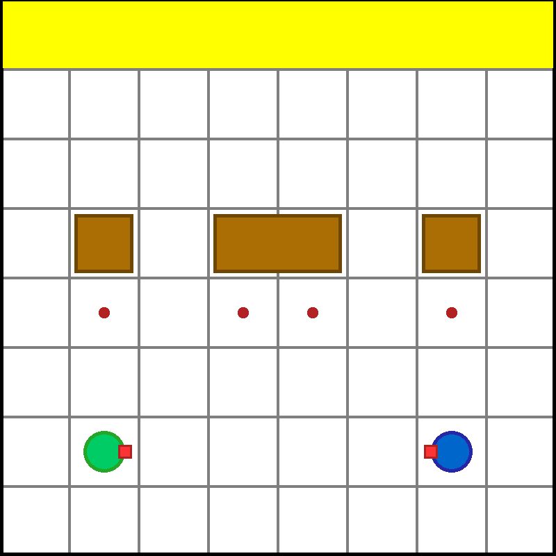
(a) (a) Box Pushing

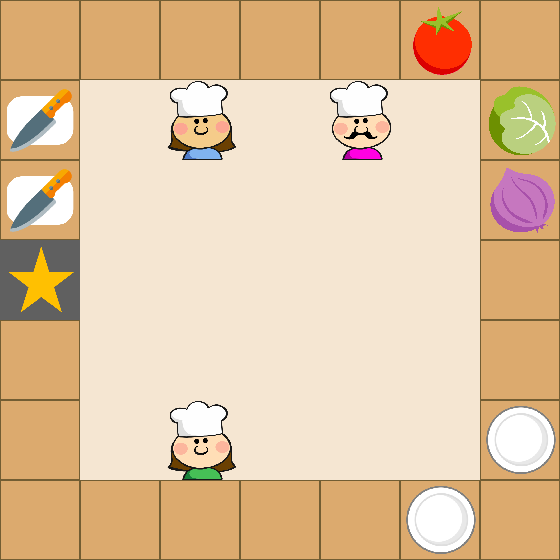
(b) (b) Overcooked-A

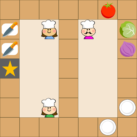
(c) (c) Overcooked-B

(d) (d) Overcooked Salad Recipe

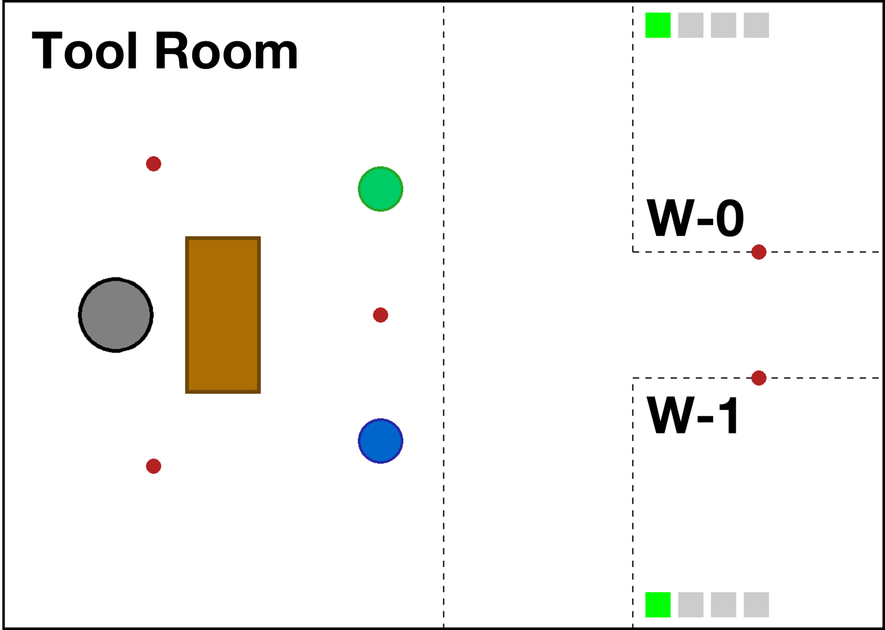
(e) (e) Warehouse-A

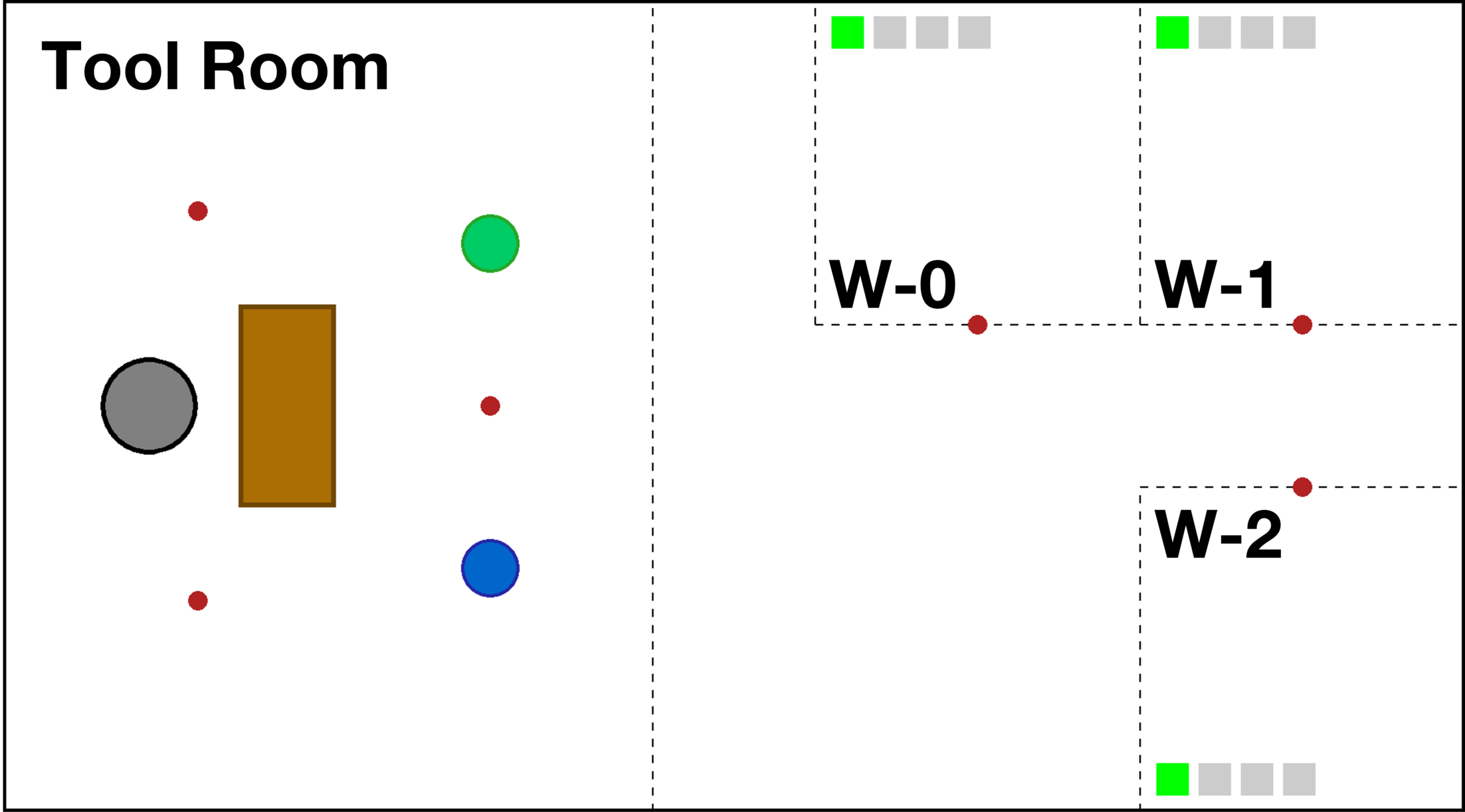
(f) (f) Warehouse-B

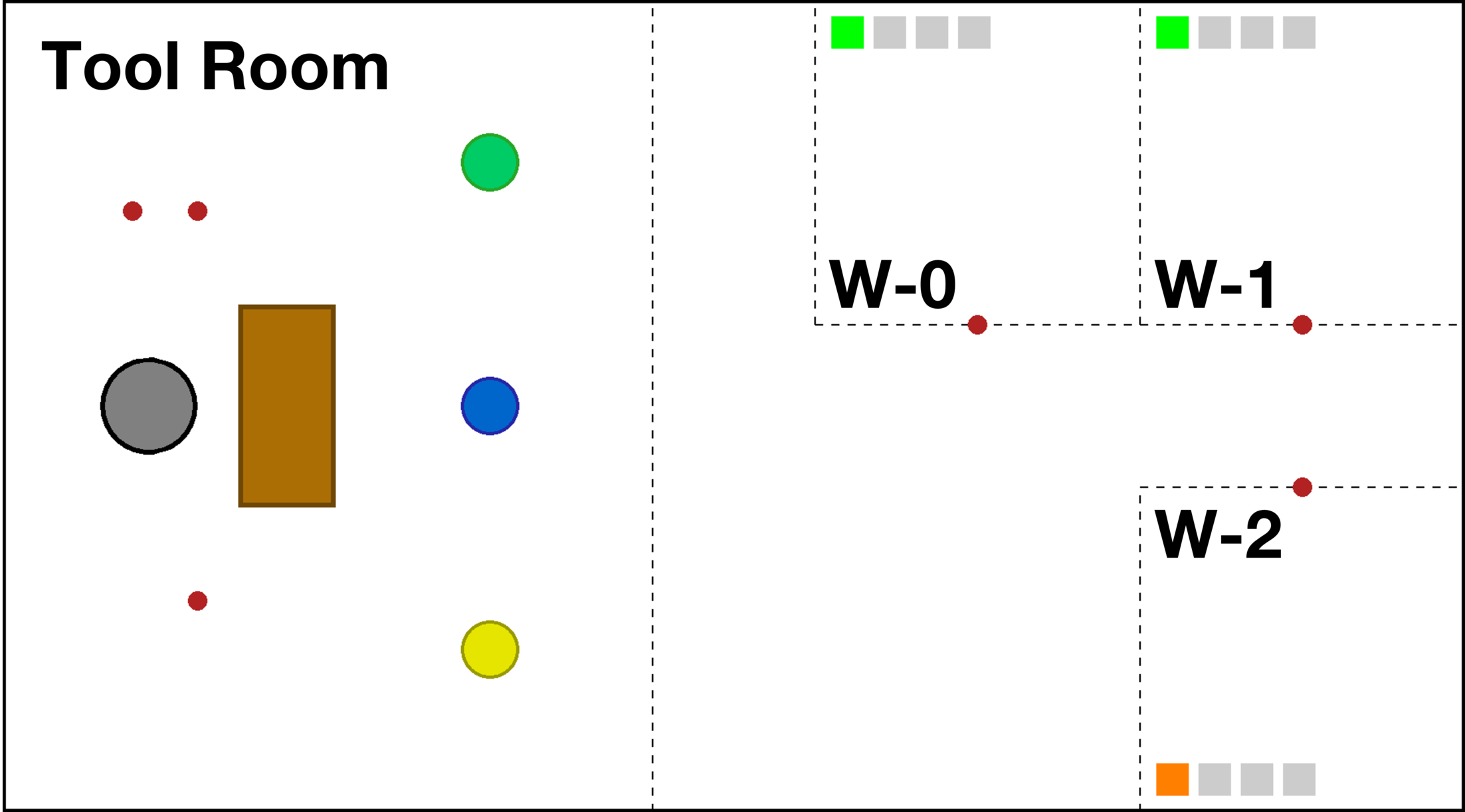
(g) (g) Warehouse-C

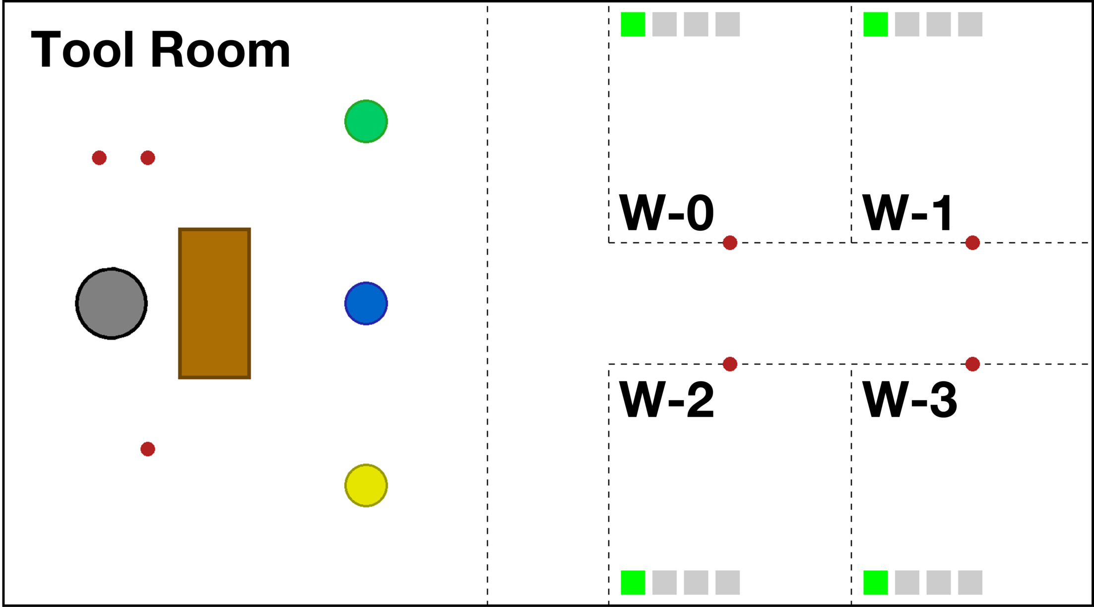
(h) (h) Warehouse-D

Figure 1: Experimental environments.

We investigate the performance of our algorithms over a variety of multi-agent problems with macro-actions (Fig. 1): Box Pushing (Xiao et al., 2019), Overcooked (Wu et al., 2021b), and a larger Warehouse Tool Delivery (Xiao et al., 2019) domain. Macro-actions are defined by using prior domain knowledge as they are straightforward in these tasks. Typically, we also include primitive-actions into macro-action set (as one-step macro-actions), which gives agents the chance to learn more complex policies that use both when it is necessary. We describe the domains’ key properties here and have more details in Appendix D.

Box Pushing (Fig. 1(a)). The optimal solution for the two agents is to cooperatively push the big box to the yellow goal area for a terminal reward, but partial observability makes this difficult. Specifically, robots have four primitive-actions: move forward, turn-left, turn-right and stay. In the macro-action case, each robot has three one-step macro-actions: Turn-left, Turn-right, and Stay, as well as three multi-step macro-actions: Move-to-small-box(i) and Move-to-big-box(i) navigate the robot to the red spot below the corresponding box and terminate with the robot facing the box; Push causes the robot to keep moving forward until arriving at the world’s boundary (potentially pushing the small box or trying to push the big one). The big box only moves if both agents push it together. Each robot can only observe the status (empty, teammate, boundary, small or big box) of the cell in front of it. A penalty is issued when any robot hits the boundary or pushes the big box alone.

Overcooked (Fig. 1(b) - 1(c)). Three agents must learn to cooperatively prepare a lettuce-tomato-onion salad and deliver it to the ‘star’ cell. The challenge is that the salad’s recipe (Fig. 1(d)) is unknown to agents. With primitive-actions (move up, down, left, right, and stay), agents can move around and achieve picking, placing, chopping and delivering by standing next to the corresponding cell and moving against it (e.g., in Fig. 1(b), the pink agent can move right and then move up to pick up the tomato). We describe the major function of macro-actions below and full details (e.g., termination conditions) are included in Appendix D.2. Each agent’s macro-action set consists of: a) five one-step macro-actions that are the same as the primitive ones; b) Chop, cuts a raw vegetable into pieces when the agent stands next to a cutting board and an unchopped vegetable is on the board, otherwise it does nothing; c) long-term navigation macro-actions: Get-Lettuce, Get-Tomato, Get-Onion, Get-Plate-1/2, Go-Cut-Board-1/2 and Deliver, which navigate the agent to the location of the corresponding object with various possible terminal effects (e.g., holding a vegetable in hand, placing a chopped vegetable on a plate, arriving at the cell next to a cutting board, delivering an item to the star cell, or immediately terminating when any property condition does not hold, e.g., no path is found or the vegetable/plate is not found); d) Go-Counter (only available in Overcook-B, Fig. 1(c)), navigates an agent to the center cell in the middle of the map when the cell is not occupied, otherwise, it moves to an adjacent cell. If the agent is holding an object or one is at the cell, the object will be placed or picked up. Each agent only observes the positions and status of the entities within a $5\times 5$ square centered on the robot.

Warehouse Tool Delivery (Fig. 1(e) - 1(h)). In each workshop (e.g., W-0), a human is working on an assembly task (involving 4 sub-tasks that each takes a number of time steps to complete) and requires three different tools for future sub-tasks to continue. A robot arm (grey) must find tools for each human on the table (brown) and pass them to mobile robots (green, blue and yellow) who are responsible for delivering tools to humans. Note that, the correct tools needed by each human are unknown to robots, which has to be learned during training in order to perform efficient delivery. A delayed delivery leads to a penalty. We consider variants with two or three mobile robots and two to four humans to examine the scalability of our methods (Fig. 1(f) - 1(h)). We also consider one faster human (orange) to check if robots can prioritize him (Fig. 1(g)). Mobile robots have the following macro-actions: Go-W(i), moves to the waypoint (red) at workshop $i$; Go-TR, goes to the waypoint at the right side of the tool room (covered by the blue robot in Fig. 1(g) and 1(h)); and Get-Tool, navigates to a pre-allocated waypoint (that is different for each robot to avoid collisions) next to the robot arm and waits there until either receiving a tool or 10 time steps have passed. The robot arm’s applicable macro-actions are: Search-Tool(i), finds tool $i$ and places it in a staging area (containing at most two tools) on the table, and otherwise, it freezes the robot for the amount of time the action would take when the area is fully occupied; Pass-to-M(i), passes the first staged tool to mobile robot $i$; and Wait-M, waits for 1 time step. The robot arm only observes the type of each tool in the staging area and which mobile robot is waiting at the adjacent waypoints. Each mobile robot always knows its position and the type of tool that it is carrying, and can observe the number of tools in the staging area or the sub-task a human is working on only when at the tool room or the workshop respectively.

4.2 Results and Discussions

We evaluate performance of one training trial with a mean discounted return measured by periodically (every 100 episodes) evaluating the learned policies over 10 testing episodes. We plot the average performance of each method over 20 independent trials with one standard error and smooth the curves over 10 neighbors. We also show the optimal expected return in Box Pushing domain as a dash-dot line. More training details are in Appendix E.

Advantages of learning with macro-actions. We first present a comparison of our macro-action-based actor-critic methods against the primitive-action-based methods in fully decentralized and fully centralized cases. We consider various grid world sizes of the Box Pushing domain (top row in Fig. 2 and two Overcooked scenarios (bottom row in Fig. 2). The results show significant performance improvements of using macro-actions over primitive-actions. More concretely, in the Box Pushing domain, reasoning about primitive movements at every time step makes the problem intractable so the robots cannot learn any good behaviors in primitive-action-based approaches other than to keep moving around. Conversely, Mac-CAC reaches near-optimal performance, enabling the robots to push the big box together. Unlike the centralized critic which can access joint information, even in the macro-action case, it is hard for each robot’s decentralized critic to correctly measure the responsibility for a penalty caused by a teammate pushing the big box alone. Mac-IAC thus converges to a local-optima of pushing two small boxes in order to avoid getting the penalty.

In the Overcooked domain, an efficient solution requires the robots to asynchronously work on independent subtasks (e.g., in scenario A, one robot gets a plate while another two robots pick up and chop vegetables; and in scenario B, the right robot transports items while the left two robots prepare the salad). This large amount of independence explains why Mac-IAC can solve the task well. This also indicates that using local information is enough for robots to achieve high-quality behaviors. As a result, Mac-CAC learns slower because it must figure out the redundant part of joint information in much larger joint macro-level history and action spaces than the spaces in the decentralized case. The primitive-action-based methods begin to learn, but perform poorly in such long-horizon tasks.

(a)

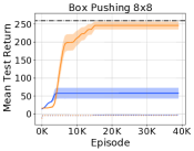
(b)

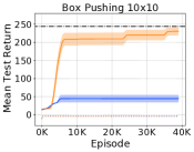
(c)

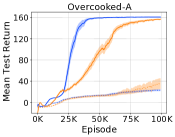
(d)

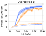
(e)

Figure 2: Decentralized learning and centralized learning with macro-actions vs primitive-actions.

Advantages of having individual centralized critics. Fig. 3 shows the evaluation of our methods in all three domains. As each agent’s observation is extremely limited in Box Pushing, we allow centralized critics in both Mac-IAICC and Naive Mac-IACC to access the state (agents’ poses and boxes’ positions), but use the joint macro-observation-action history in the other two domains.

In the Box Pushing task (the left two in the top row in Fig. 3), Naive Mac-IACC (green) can learn policies almost as good as the ones for Mac-IAICC (red) for the smaller domain, but as the grid world size grows, Naive Mac-IACC performs poorly while Mac-IAICC keeps its performance near the centralized approach. From each agent’s perspective, the bigger the world size is, the more time steps a macro-action could take, and the less accurate the critic of Naive Mac-IACC becomes since it is trained depending on any agent’s macro-action termination. Conversely, Mac-IAICC gives each agent a separate centralized critic trained with the reward associated with its own macro-action execution.

In Overcooked-A (the third one at the top row in Fig. 3), as Mac-IAICC’s performance is determined by the training of three agents’ critics, it learns slower than Naive Mac-IACC in the early stage but converges to a slightly higher value and has better learning stability than Naive Mac-IACC in the end. The result of scenario B (the last one at the top row in Fig. 3) shows that Mac-IAICC outperforms other methods in terms of achieving better sample efficiency, a higher final return and a lower variance. The middle wall in scenario B limits each agent’s moving space and leads to a higher frequency of macro-action terminations. The shared centralized critic in Naive Mac-IACC thus provides more noisy value estimations for each agent’s actions. Because of this, Naive Mac-IACC performs worse with more variance. Mac-IAICC, however, does not get hurt by such environmental dynamics change. Both Mac-CAC and Mac-IAC are not competitive with Mac-IAICC in this domain.

In the Warehouse scenarios (the bottom row in Fig. 3), Mac-IAC (blue) performs the worst due to its natural limitations and the domain’s partial observability. In particular, it is difficult for the gray robot (arm) to learn an efficient way to find the correct tools purely based on local information and very delayed rewards that depend on the mobile robots’ behaviors. In contrast, in the fully centralized Mac-CAC (orange), both the actor and the critic have global information so it can learn faster in the early training stage. However, Mac-CAC eventually gets stuck at a local-optimum in all five scenarios due to the exponential dimensionality of joint history and action spaces over robots. By leveraging the CTDE paradigm, both Mac-IAICC and Naive Mac-IACC perform the best in warehouse A. Yet, the weakness of Naive Mac-IACC is clearly exposed when the problem is scaled up in Warehouse B, C and D. In these larger cases, the robots’ asynchronous macro-action executions (e.g., traveling between rooms) become more complex and cause more mismatching between the termination from each agent’s local perspective and the termination from the centralized perspective, and therefore, Naive Mac-IACC’s performance significantly deteriorates, even getting worse than Mac-IAC in Warehouse-D. In contrast, Mac-IAICC can maintain its outstanding performance, converging to a higher value with much lower variance, compared to other methods. This outcome confirms not only Mac-IAICC’s scalability but also the effectiveness of having an individual critic for each agent to handle variable degrees of asynchronicity in agents’ high-level decision-making.

(a)

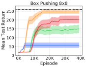
(b)

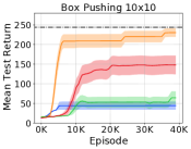
(c)

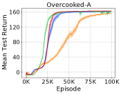
(d)

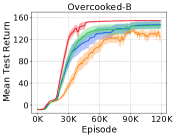
(e)

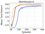
(f)

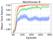
(g)

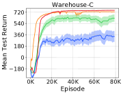
(h)

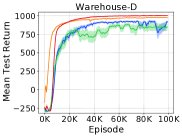
(i)

Figure 3: Comparison of macro-action-based asynchronous actor-critic methods.

(a)

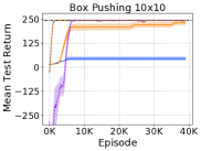
(b)

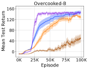
(c)

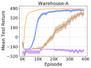
(d)

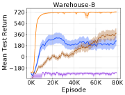
(e)

Figure 4: Comparisons of macro-action-based actor-critic methods and value-based methods.

Comparative analysis between actor-critic and value-based approaches. We also compare our actor-critic methods (Mac-IAC and Mac-CAC) with the current state-of-the-art asynchronous decentralized and centralized MARL methods, the value-based approaches (Mac-Dec-Q and Mac-Cen-Q) (Xiao et al., 2019), shown in Fig. 4. The Box Pushing task requires agents to simultaneously reach the big box and push it together. This consensus is rarely achieved when agents independently sample actions using stochastic policies in Mac-IAC and is hard to learn from pure on-policy data. By having a replay-buffer, value-based approaches show much stronger sample efficiency than on-policy actor-critic approaches in this domain with a small action space (left figure). Such an advantage is sustained by the decentralized value-based method (Mac-Dec-Q) but gets lost in the centralized one (Mac-Cen-Q) in the Overcooked domains due to a huge joint macro-action space ($15^{3}$). On the contrary, our actor-critic methods can scale to large domains and learn high-quality solutions. This is particularly noticeable on Warehouse-A, where the policy gradient methods quickly learn a high-quality policy while the centralized Mac-Cen-Q is slow to learn and the decentralized Mac-Dec-Q is unable to learn. In addition, the stochastic policies in actor-critic methods potentially have better exploration property so that, in Warehouse domains, Mac-IAC can bypass an obvious local-optima that Mac-Dec-Q falls into, where the robot arm greedily chooses Wait-M to avoid more penalties.

5 Hardware Experiments

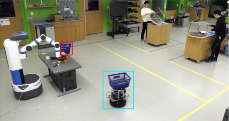
(a) (a)

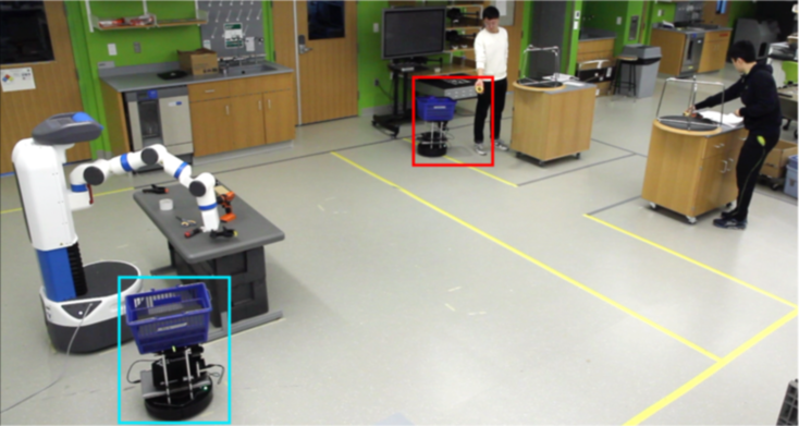
(b) (b)

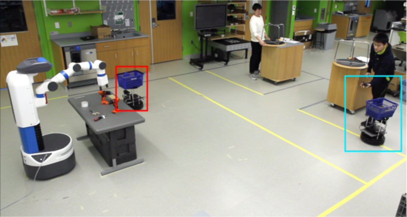
(c) (c)

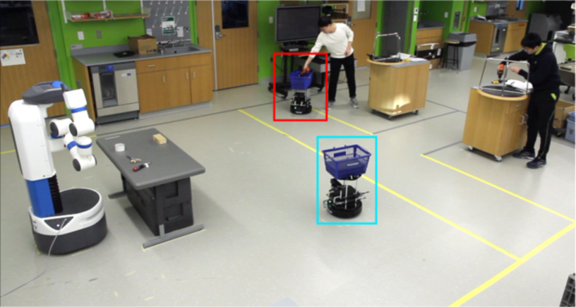
(d) (d)

Figure 5: Collaborative behaviors generated by running the decentralized policies learned by Mac-IAICC where Turtlebot-0 (T-0) is bounded in red and Turtlebot-1 (T-1) is bounded in blue. (a) After staging a tape measure at the left, Fetch looks for the 2nd one while Turtlebots approach the table; (b) T-0 deliveries a tap measure to W-0 and T-1 waits for a clamp from Fetch; (c) T-1 deliveries a clamp to W-1, while T-0 carries the other clamp and goes to W-0, and Fetch searches for an electric drill; (d) T-0 deliveries an electric drill (the last tool) to W-0 and the entire delivery task is completed.

We also extend scenario A of the Warehouse Tool Delivery task to a hardware domain (details of experimental setup are referred to Appendix F). Fig. 5 shows the sequential collaborative behaviors of the robots in one hardware trial. Fetch was able to find tools in parallel such that two tape measures (Fig. 5(a)), two clamps (Fig. 5(b)) and two electric drills, were found instead of finding all three types of tool for one human and then moving on to the other which would result in one of the humans waiting. Fetch’s efficiency is also reflected in the behaviors such that it passed a tool to the Turtelbot who arrived first (Fig. 5(b)) and continued to find the next tool when there was no Turtlebot waiting beside it (Fig. 5(c)). Meanwhile, Turtlebots were clever such that they successfully avoid delayed delivery by sending tools one by one to the nearby workshop (e.g., T-0 focused on W-0 shown in Fig. 5(b) and 5(d), and T-1 focused on W-1 shown in Fig. 5(c)), rather than waiting for all tools before delivering, traveling a longer distance to serve the human at the diagonal, or prioritizing one of the humans altogether.

6 Conclusion

This paper introduces a general formulation for asynchronous multi-agent macro-action-based policy gradients under partial observability along with proposing a decentralized actor-critic method (Mac-IAC), a centralized actor-critic method (Mac-CAC), and two CTDE-based actor-critic methods (Naive Mac-IACC and Mac-IAICC). These are the first approaches to be able to incorporate controllers that may require different amounts of time to complete (macro-actions) in a general asynchronous multi-agent actor-critic framework. Empirically, our methods are able to learn high-quality macro-action-based policies allowing agents to perform asynchronous collaborations in large and long-horizon problems. Importantly, our most advanced method, Mac-IAICC, allows agents to have individual centralized critics tailored to the agent’s own macro-action execution. Additionally, the practicality of our approach is validated in a real-world multi-robot setup based on a warehouse domain. This work provides a foundation for future macro-action-based MARL algorithm development, including other policy gradient-based methods as well as methods which also learn the macro-actions.

Appendix A Related Work

MARL has been used for solving multi-robot problems Alon and Zhou [2020], Khan et al. [2019], Mitchell et al. [2020], Park et al. [2020], Stone et al. [2005], Strickland et al. [2019], Tang [2019] and hierarchy has also been introduced into multi-robot scenarios Chen [2014], Luo et al. [2018], Oliehoek and Visser [2006], Omidshafiei et al. [2017b], Zhang et al. [2017], but hierarchical MARL is still novel for multi-robot systems Nachum et al. [2019], Wang et al. [2020b], Wu et al. [2021a], Xiao et al. [2019].

One line of hierarchical MARL is still focusing on learning primitive-action-based policy for each agent, while leveraging a hierarchical structure to achieve knowledge transfer Yang et al. [2021], credit assignment Ahilan and Dayan [2019] and low-level policy factorization over agents Vezhnevets et al. [2020]. In these works, as the decision-making over agents is still limited at a single low-level, none of them has been evaluated in large-scale realistic domains. Instead, by having macro-actions, our methods equip agents with the potential capability of exploiting abstracted skills, sub-task allocation and problem decomposition via hierarchical decision-making, which is critical for scaling up to real-world multi-robot tasks.

Another line of the research allow agents to learn both a high-level policy and a low-level policy, but the methods either force agents to perform a high-level choice at every time step de Witt et al. [2019], Han et al. [2019] or require all agents’ high-level decisions have the same time duration Nachum et al. [2019], Wang et al. [2020b, 2021b], Xu et al. [2021], Yang et al. [2020b], where agents are actually synchronized at both levels. In contrast, our frameworks are more general and applicable to real-world multi-robot systems because they allow agents to asynchronously execute at a high-level without synchronization or waiting for all agents to terminate.

Recently, some asynchronous hierarchical approaches have been developed. Xiao et al. [2019] and Wu et al. [2021a] extend DQN Mnih et al. [2015] to learn macro-action-value functions and spatial-action-value maps for agents respectively. Our work, however, focuses on policy gradient algorithms that have different theoretical properties than value-based approaches (e.g., our methods are more scalable in the action space). Both classes of methods can co-exit and fit well with different sets of tasks. Menda et al. [2019] frame multi-agent asynchronous decision-making problems as event-driven processes with one assumption on the acceptable of losing the ability to capture low-level interaction between agents within an event duration and the other on homogeneous agents, but our frameworks rely on the time-driven simulator used for general multi-agent and single-agent RL problems and do not have the above assumptions. Chakravorty et al. [2019] adapt a single-agent option-critic framework Bacon et al. [2017] to multi-agent domains to learn all components (e.g., low-level policy, high-level abstraction, high-level policy) from scratch, but learning at both levels is difficult and the proposed method does not perform well even in small TeamGrid Maxime and Julien [2020] scenarios. More important to note is that none of the existing works provides a principled way for directly optimizing parameterized macro-action-based policies via asynchronous policy gradients to solve general multi-agent problems with macro-actions, and our work in this paper seeks to fill this gap.

Appendix B Macro-Action-Based Policy Gradient Theorem

As POMDPs can always be transformed to history-based MDPs, we can directly adapt the general Bellman equation for the state values of a hierarchical policy [Sutton et al., 1999] to a macro-action-based POMDP by replacing the state $s$ with a history $h$ as follows (for keeping the notaion simple, we use $\tau$ to represent the number of timesteps taken by the corresponding macro-action $m$, and we use $h$ to represent macro-observation-action history):

$$V^{\Psi}(h)=\sum_{m}\Psi(m|h)Q^{\Psi}(h,m)$$ (8)

$$Q^{\Psi}(h,m)=r^{c}(h,m)+\sum_{h^{\prime}}P(h^{\prime}|h,m)V^{\Psi}(h^{\prime})$$ (9)

where,

$$r^{c}(h,m)=\mathbb{E}_{\tau\sim\beta_{m},s_{t_{m}}|h}\Big{[}\sum_{t=t_{m}}^{t_{m}+\tau-1}\gamma^{t}r_{t}\Big{]}$$ (10)

$$P(h^{\prime}|h,m)=P(z^{\prime}|h,m) =\sum_{\tau=1}^{\infty}\gamma^{\tau}P(z^{\prime},\tau|h,m)$$ (11)

$$=\sum_{\tau=1}^{\infty}\gamma^{\tau}P(\tau|h,m)P(z^{\prime}|h,m,\tau)$$ (12)

$$=\sum_{\tau=1}^{\infty}\gamma^{\tau}P(\tau|h,m)P(z^{\prime}|h,m,\tau)$$ (13)

$$=\mathbb{E}_{\tau\sim\beta_{m}}\Big{[}\gamma^{\tau}\mathbb{E}_{s|h}\big{[}\mathbb{E}_{s^{\prime}|s,m,\tau}[P(z^{\prime}|m,s^{\prime})]\big{]}\Big{]}$$ (14)

Next, we follow the proof of the policy gradient theorem [Sutton et al., 2000]:

$$\nabla_{\theta}V^{\Psi_{\theta}}(h) =\nabla_{\theta}\Biggr{[}\sum_{m}\Psi_{\theta}(m|h)Q^{\Psi_{\theta}}(h,m)\Biggr{]}$$ (15)

$$=\sum_{m}\Big{[}\nabla_{\theta}\Psi_{\theta}(m|h)Q^{\Psi_{\theta}}(h,m)+\Psi_{\theta}(m|h)\nabla_{\theta}Q^{\Psi_{\theta}}(h,m)\Big{]}$$ (16)

$$=\sum_{m}\Big{[}\nabla_{\theta}\Psi_{\theta}(m|h)Q^{\Psi_{\theta}}(h,m)+\Psi_{\theta}(m|h)\nabla_{\theta}\big{(}r^{c}(h,m)+\sum_{h^{\prime}}P(h^{\prime}|h,m)V^{\Psi_{\theta}}(h^{\prime})\big{)}\Big{]}$$ (17)

$$=\sum_{m}\Big{[}\nabla_{\theta}\Psi_{\theta}(m|h)Q^{\Psi_{\theta}}(h,m)+\Psi_{\theta}(m|h)\sum_{h^{\prime}}P(h^{\prime}|h,m)\nabla_{\theta}V^{\Psi_{\theta}}(h^{\prime})\big{)}\Big{]}$$ (18)

$$=\sum_{\hat{h}\in H}\sum_{k=0}^{\infty}P(h\rightarrow\hat{h},k,\Psi_{\theta})\sum_{m}\nabla_{\theta}\Psi_{\theta}(m|\hat{h})Q^{\Psi_{\theta}}(\hat{h},m)\,\,\,\,(\text{after repeated unrolling})$$ (19)

Then, we can have:

$$\nabla_{\theta}J(\theta) =\nabla_{\theta}V^{\Psi_{\theta}}(h_{0})$$ (20)

$$=\sum_{h\in H}\sum_{k=0}^{\infty}P(h_{0}\rightarrow h,k,\Psi_{\theta})\sum_{m}\nabla_{\theta}\Psi_{\theta}(m|h)Q^{\Psi_{\theta}}(h,m)$$ (21)

$$=\sum_{h}\rho^{\Psi_{\theta}}(h)\sum_{m}\nabla_{\theta}\Psi_{\theta}(m|h)Q^{\Psi_{\theta}}(h,m)$$ (22)

$$=\sum_{h}\rho^{\Psi_{\theta}}(h)\sum_{m}\Psi_{\theta}(m|h)\nabla_{\theta}\log\Psi_{\theta}(m|h)Q^{\Psi_{\theta}}(h,m)$$ (23)

$$=\mathbb{E}_{h\sim\rho^{\Psi_{\theta}},m\sim\Psi_{\theta}}\Big{[}\nabla_{\theta}\log\Psi_{\theta}(m|h)Q^{\Psi_{\theta}}(h,m)\Big{]}$$ (24)

Appendix C Asynchronous Acotr-Critic Algorithms

In this section, we present the pesudo code of each proposed macro-action-based actor-critic algorithm with an example to show how the sequential experiences are squeezed for training the critic and the actor. We describe all methods in the on-policy learning manner while off-policy learning can be achieved by applying importance sampling weights and not resetting the buffer.

Macro-Action-Based Independent Actor-Critic (Mac-IAC):

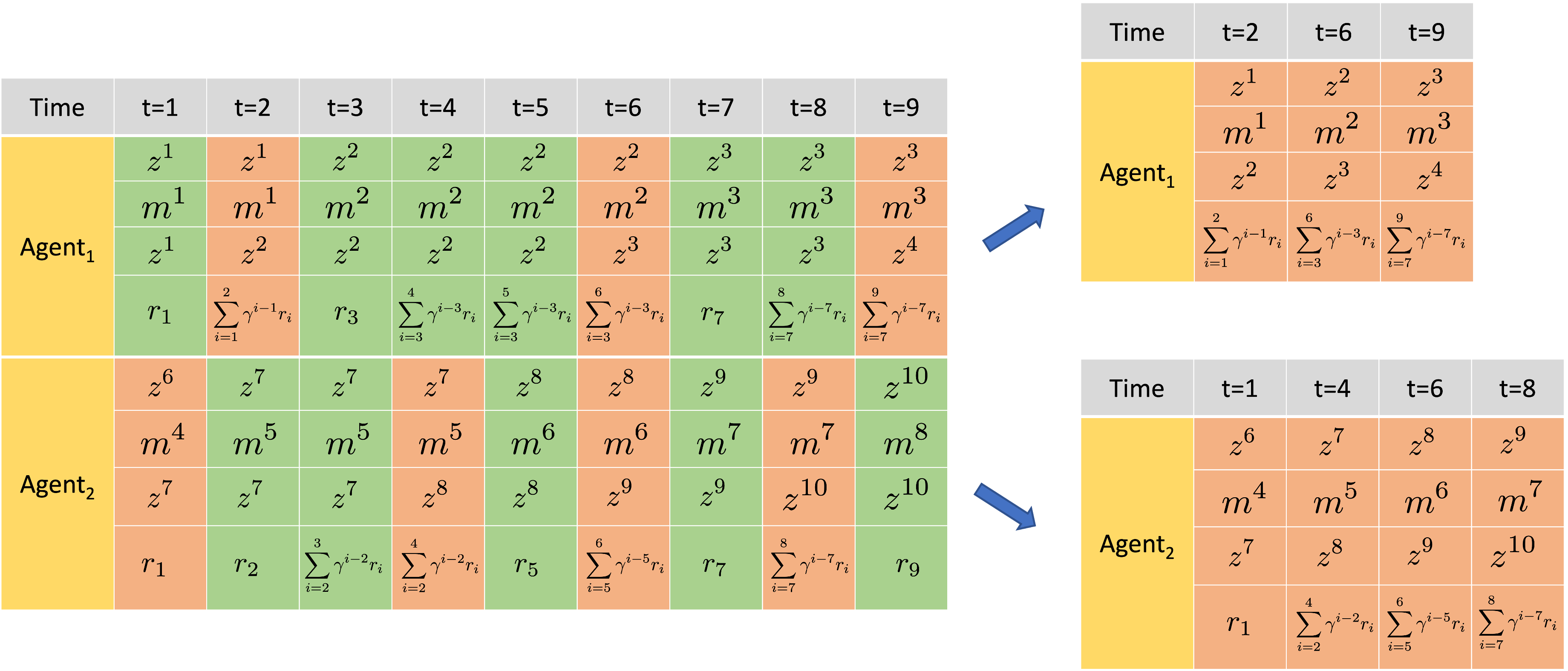
Figure 6: An example of the trajectory squeezing process in Mac-IAC. We collect each agent’s high-level transition tuple at every primitive-step. Each agent is allowed to obtain a new macro-observation if and only if the current macro-action terminates, otherwise, the next macro-observation is set as same as the previous one. Each agent separately squeezes its sequential experiences by picking out the transitions when its macro-action terminates (red cells). Each agent independently train the critic and the policy using the squeezed trajectory.

Algorithm 1 Mac-IAC

1:Initialize a decentralized policy network for each agent $i$: $\Psi_{\theta_{i}}$

2:Initialize decentralized critic networks for each agent $i$: $V_{\mathbf{w}_{i}}^{\Psi_{\theta_{i}}}$, $V_{\mathbf{w}_{i}^{-}}^{\Psi_{\theta_{i}}}$

3:Initialize a buffer $\mathcal{D}$

4:for episode = $1$ to $M$ do

5:    $t=0$

6:    Reset env

7:    while not reaching a terminal state and $t<\mathbb{H}$ do

8:        $t\leftarrow t+1$

9:        for each agent $i$ do

10:           if the macro-action $m_{i}$ is terminated then

11:               $m_{i}\sim\Psi_{\theta_{i}}(\cdot\mid h_{i};\epsilon)$

12:           else

13:               Continue running current macro-action $m_{i}$                    

14:        for each agent $i$ do

15:           Get cumulative reward $r^{c}_{i}$, next macro-observation $z^{\prime}_{i}$

16:           Collect $\langle z_{i},m_{i},z^{\prime}_{i},r^{c}_{i}\rangle$ into the buffer $\mathcal{D}$             

17:    if episode mod $I_{\text{train}}=0$ then

18:        for each agent $i$ do

19:           Squeeze agent $i$’s trajectories in the buffer $\mathcal{D}$

20:           Perform a gradient decent step on $L(\mathbf{w}_{i})=\big{(}y-V^{\Psi_{\theta_{i}}}_{\mathbf{w}_{i}}(h_{i})\big{)}^{2}_{\mathcal{D}}$, where $y=r^{c}_{i}+\gamma^{\tau_{m_{i}}}V^{\Psi_{\theta_{i}}}_{\mathbf{w}_{i}^{-}}(h_{i}^{\prime})$

21:           Perform a gradient ascent on:

22:           $\nabla_{\theta_{i}}J(\theta_{i})=\mathbb{E}_{\vec{\Psi}_{\vec{\theta}}}\Big{[}\nabla_{\theta_{i}}\log\Psi_{\theta_{i}}(m_{i}|h_{i})\big{(}r^{c}_{i}+\gamma^{\tau_{m_{i}}}V^{\Psi_{\theta_{i}}}_{\mathbf{w}_{i}^{-}}(h_{i}^{\prime})-V^{\Psi_{\theta_{i}}}_{\mathbf{w}_{i}}(h_{i})\big{)}\Big{]}$         

23:        Reset buffer $\mathcal{D}$     

24:    if episode mod $I_{\text{TargetUpdate}}=0$ then

25:        for each agent $i$ do

26:           Update the critic target network $\mathbf{w}_{i}^{-}\leftarrow\mathbf{w}_{i}$             

Macro-Action-Based Centralized Actor-Critic (Mac-CAC):

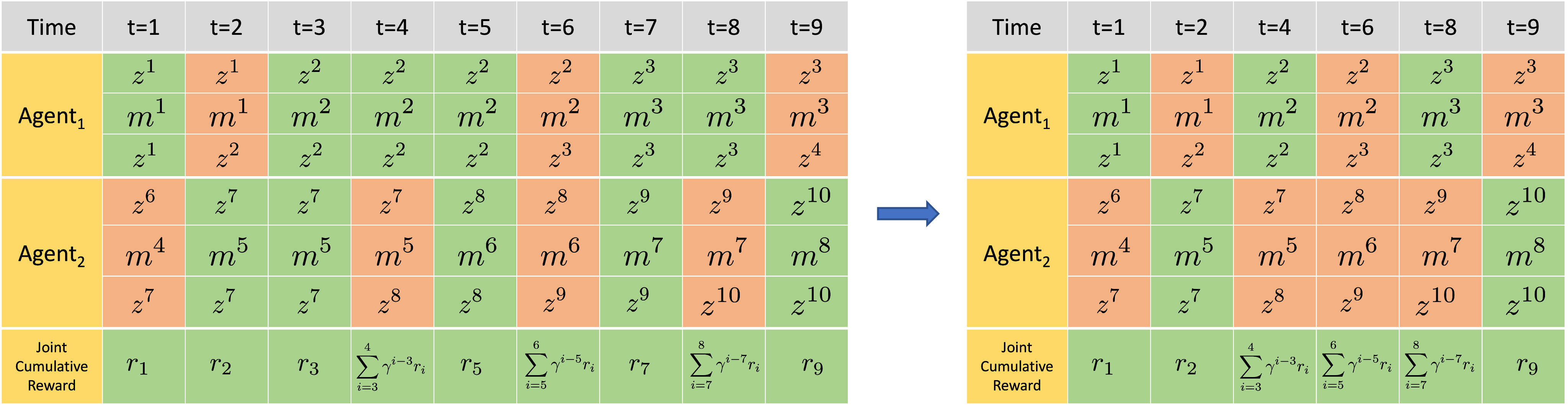
Figure 7: An example of the trajectory squeezing process in Mac-CAC. Joint sequential experiences are squeezed by picking out joint transition tuples when the joint macro-action terminates, in that, $any$ agent’s macro-action termination (marked in red) ends the joint macro-action at the timestep. For example, at $t=1$, agents execute a joint macro-action $\vec{m}=\langle m^{1},m^{4}\rangle$ for one timestep; at $t=2$, the joint macro-action becomes $\langle m^{1},m^{5}\rangle$ as $\text{Agent}_{2}$ finished $m^{4}$ at last step and chooses a new macro-action $m^{5}$; $\text{Agent}_{1}$ finished its macro-action $m_{1}$ at $t=2$ and selects a new macro-action $m^{2}$ at $t=3$ so that the joint macro-action switches to $\langle m^{2},m^{5}\rangle$ which keeps running until the 4th timestep. Therefore, the first two joint macro-actions have two single-step reward respectively, and reward of joint macro-action $\langle m^{2},m^{5}\rangle$ is an accumulative reward over two consecutive timesteps.

Algorithm 2 Mac-CAC

1:Initialize a centralized policy network: $\Psi_{\theta}$

2:Initialize centralized critic networks: $V_{\mathbf{w}}^{\Psi_{\theta}}$, $V_{\mathbf{w}^{-}}^{\Psi_{\theta}}$

3:Initialize a centralized buffer $\mathcal{D}\leftarrow\text{Mac-JERTs}$,

4:for episode = $1$ to $M$ do

5:    $t=0$

6:    Reset env

7:    while not reaching a terminal state and $t<\mathbb{H}$ do

8:        $t\leftarrow t+1$

9:        if the joint macro-action $\vec{m}$ is terminated then

10:           $\vec{m}\sim\Psi_{\theta}(\cdot\mid\vec{h},\vec{m}^{\text{undone}};\epsilon)$

11:        else

12:           Continue running current joint macro-action $\vec{m}$         

13:        Get a joint cumulative reward $\vec{r\,}^{c}$, next joint macro-observation $\vec{z\,}^{\prime}$

14:        Collect $\langle\vec{z},\vec{m},\vec{z\,}^{\prime},\vec{r\,}^{c}\rangle$ into the buffer $\mathcal{D}$     

15:    if episode mod $I_{\text{train}}=0$ then

16:        Squeeze joint macro-level trajectories in the buffer $\mathcal{D}$ according to joint macro-action terminations

17:        Perform a gradient decent step on $L(\mathbf{w})=\big{(}y-V^{\Psi_{\theta}}_{\mathbf{w}}(\vec{h})\big{)}^{2}_{\mathcal{D}}$, where $y=\vec{r\,}^{c}+\gamma^{\vec{\tau}_{\vec{m}}}V^{\Psi_{\theta}}_{\mathbf{w}^{-}}(\vec{h}^{\prime})$

18:        Perform a gradient ascent on $\nabla_{\theta}J(\theta)=\mathbb{E}_{\Psi_{\theta}}\Big{[}\nabla_{\theta}\log\Psi_{\theta}(\vec{m}\mid\vec{h})\big{(}\vec{r\,}^{c}+\gamma^{\vec{\tau}_{\vec{m}}}V^{\Psi_{\theta}}_{\mathbf{w}^{-}}(\vec{h}^{\prime})-V^{\Psi_{\theta}}_{\mathbf{w}}(\vec{h})\big{)}\Big{]}$

19:        Reset buffer $\mathcal{D}$     

20:    if episode mod $I_{\text{TargetUpdate}}=0$ then

21:        Update the critic target network $\mathbf{w}^{-}\leftarrow\mathbf{w}$     

where, $\vec{m}^{\text{undone}}$ is the sub-joint-macro-action over the agents who have not terminated their macro-actions and will continue running.

Naive Mac-IACC:

In the pseudo code of Naive Mac-IACC presented below, we assume the accessible centralized information $\mathbf{x}$ is joint macro-observation-action history in the centralized critic.

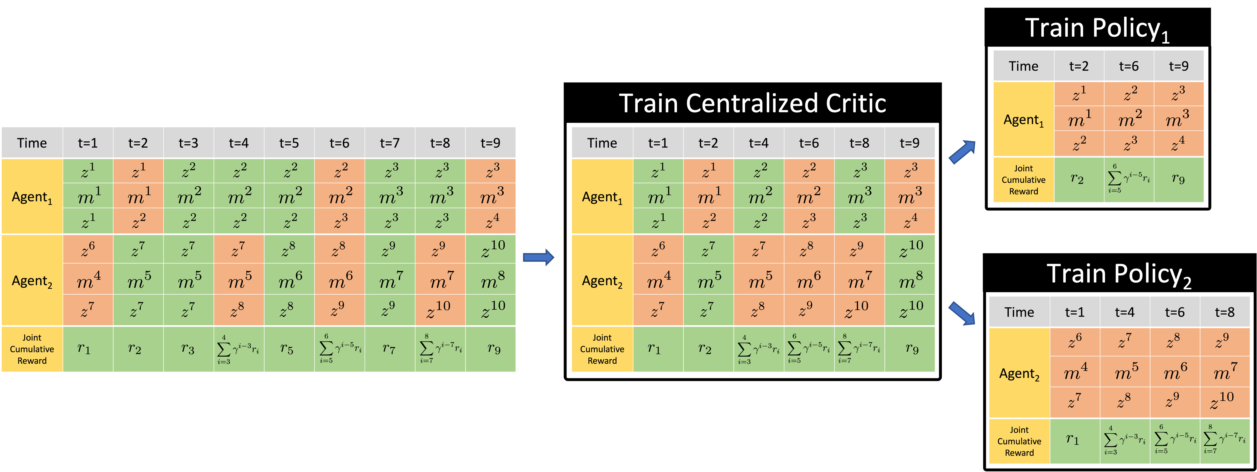
Figure 8: An example of the trajectory squeezing process in Navie Mac-IACC.The joint trajectory is first squeezed depending on joint macro-action termination for training the centralized critic (line 18-19 in Algorithm 3). Then, the trajectory is further squeezed for each agent depending on each agent’s own macro-action termination for training the decentralized policy (line 20-23 in Algorithm 3).

Algorithm 3 Naive Mac-IACC

1:Initialize a decentralized policy network for each agent $i$: $\Psi_{\theta_{i}}$

2:Initialize centralized critic networks: $V_{\mathbf{w}}^{\vec{\Psi}_{\vec{\theta}}}$, $V_{\mathbf{w}^{-}}^{\vec{\Psi}_{\vec{\theta}}}$

3:Initialize a decentralized buffer $\mathcal{D}\leftarrow\text{Mac-JERTs}$,

4:for episode = $1$ to $M$ do

5:    $t=0$

6:    Reset env

7:    while not reaching a terminal state and $t<\mathbb{H}$ do

8:        $t\leftarrow t+1$

9:        for each agent $i$ do

10:           if the macro-action $m_{i}$ is terminated then

11:               $m_{i}\sim\Psi_{\theta_{i}}(\cdot\mid h_{i};\epsilon)$

12:           else

13:               Continue running current macro-action $m_{i}$                    

14:        Get a reward $\vec{r\,}^{c}$ accumulated based on current joint macro-action termination

15:        Get next joint macro-observations $\vec{z\,}^{\prime}$

16:        Collect $\langle\vec{z},\vec{m},\vec{z\,}^{\prime},\vec{r\,}^{c}\rangle$ into the buffer $\mathcal{D}$     

17:    if episode mod $I_{\text{train}}=0$ then

18:        Squeeze joint macro-level trajectories in the buffer $\mathcal{D}$ according to joint macro-action terminations

19:        Perform a gradient decent step on $L(\mathbf{w})=\big{(}y-V^{\vec{\Psi}_{\vec{\theta}}}_{\mathbf{w}}(\vec{h})\big{)}^{2}_{\mathcal{D}}$, where $y=\vec{r\,}^{c}+\gamma^{\vec{\tau}_{\vec{m}}}V^{\vec{\Psi}_{\vec{\theta}}}_{\mathbf{w}^{-}}(\vec{h}^{\prime})$

20:        for each agent $i$ do

21:           Squeeze agent $i$’s trajectories in the buffer $\mathcal{D}$ according to its own macro-action terminations

22:           Perform a gradient ascent on:

23:           $\nabla_{\theta_{i}}J(\theta_{i})=\mathbb{E}_{\vec{\Psi}_{\vec{\theta}}}\Big{[}\nabla_{\theta_{i}}\log\Psi_{\theta_{i}}(m_{i}|h_{i})\big{(}\vec{r\,}^{c}+\gamma^{\vec{\tau}_{\vec{m}}}V^{\vec{\Psi}_{\vec{\theta}}}_{\mathbf{w}^{-}}(\vec{h}^{\prime})-V^{\vec{\Psi}_{\vec{\theta}}}_{\mathbf{w}}(\vec{h})\big{)}\Big{]}$         

24:        Reset buffer $\mathcal{D}$     

25:    if episode mod $I_{\text{TargetUpdate}}=0$ then

26:        Update the critic target network $\mathbf{w}^{-}\leftarrow\mathbf{w}$     

Macro-Action-Based Independent Actor with Individual Centralized Critic (Mac-IAICC):

In the pseudo code of Mac-IAICC presented below, we assume the accessible centralized information $\mathbf{x}$ is joint macro-observation-action history in the centralized critic.

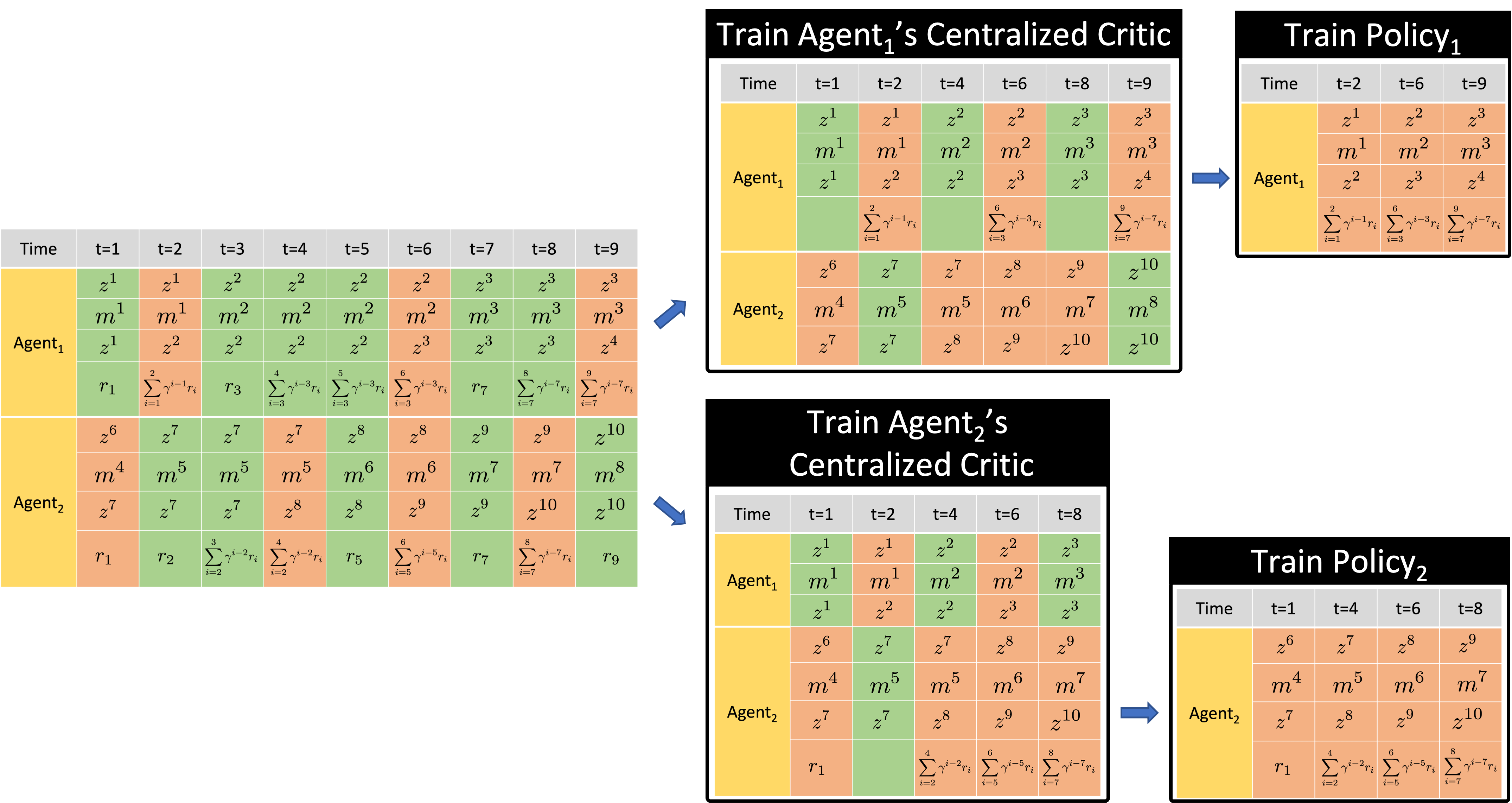
Figure 9: An example of the trajectory squeezing process in Mac-IAICC: each agent learns an individual centralized critic for the decentralized policy optimization. In order to achieve a better use of centralized information, the recurrent layer in each critic’s neural network should receive all the valid joint macro-observation-action information (when $any$ agent terminates its macro-action (line 20-22) and obtain a new joint macro-observation). However, the critic’s TD updates and the policy’s updates still rely on each agent’s individual macro-action termination and the accumulative reward at the corresponding timestep (line 23-26). Hence, the trajectory squeezing process for training each critic still depends on joint-macro-action termination but only retaining the accumulative rewards w.r.t. the corresponding agent’s macro-action termination for computing the TD loss (the middle part in the above picture). Then, each agent’s trajectory is further squeezed depending on its macro-action termination to update the decentralized policy.

Algorithm 4 Mac-IAICC

1:Initialize a decentralized policy network for each agent $i$: $\Psi_{\theta_{i}}$

2:Initialize centralized critic networks for each agent $i$: $V_{\mathbf{w}_{i}}^{\vec{\Psi}_{\vec{\theta}}}$, $V_{\mathbf{w}^{-}_{i}}^{\vec{\Psi}_{\vec{\theta}}}$

3:Initialize a decentralized buffer $\mathcal{D}$

4:for episode = $1$ to $M$ do

5:    $t=0$

6:    Reset env

7:    while not reaching a terminal state and $t<\mathbb{H}$ do

8:        $t\leftarrow t+1$

9:        for each agent $i$ do

10:           if the macro-action $m_{i}$ is terminated then

11:               $m_{i}\sim\Psi_{\theta_{i}}(\cdot\mid h_{i};\epsilon)$

12:           else

13:               Continue running current macro-action $m_{i}$                    

14:        for each agent $i$ do

15:           Get a reward $r^{c}_{i}$ accumulated based on agent $i$’s macro-action termination         

16:        Get next joint macro-observations $\vec{z\,}^{\prime}$

17:        Collect $\langle\vec{z},\vec{m},\vec{z\,}^{\prime},\{r^{c}_{1},\dots,r^{c}_{n}\}\rangle$ into the buffer $\mathcal{D}$     

18:    if episode mod $I_{\text{train}}=0$ then

19:        for each agent $i$ do

20:           Squeeze trajectories in the buffer $\mathcal{D}$ according to joint macro-action terminations

21:           Compute the TD-error of each timestep in the squeezed experiences:

22:           $L(\mathbf{w}_{i})=\big{(}y-V^{\vec{\Psi}_{\vec{\theta}}}_{\mathbf{w}_{i}}(\vec{h})\big{)}^{2}_{\mathcal{D}}$, where $y=r^{c}_{i}+\gamma^{\tau_{m_{i}}}V^{\vec{\Psi}_{\vec{\theta}}}_{\mathbf{w}^{-}_{i}}(\vec{h}^{\prime})$

23:           Perform a gradient descent only over the TD-errors when agent $i$’s macro-action is terminated

24:           Squeeze agent $i$’s trajectories in the buffer $\mathcal{D}$ according to its own macro-action terminations

25:           Perform a gradient ascent on:

26:           $\nabla_{\theta_{i}}J(\theta_{i})=\mathbb{E}_{\vec{\Psi}_{\vec{\theta}}}\Big{[}\nabla_{\theta_{i}}\log\Psi_{\theta_{i}}(m_{i}|h_{i})\big{(}r^{c}_{i}+\gamma^{\tau_{m_{i}}}V^{\vec{\Psi}_{\vec{\theta}}}_{\mathbf{w}^{-}_{i}}(\vec{h}^{\prime})-V^{\vec{\Psi}_{\vec{\theta}}}_{\mathbf{w}_{i}}(\vec{h})\big{)}\Big{]}$         

27:        Reset buffer $\mathcal{D}$     

28:    if episode mod $I_{\text{TargetUpdate}}=0$ then

29:        for each agent $i$ do

30:           Update the critic target network $\mathbf{w}_{i}^{-}\leftarrow\mathbf{w}_{i}$             

Appendix D Domain Descriptions and Results

D.1 Box Pushing

(a) (a) 8x8

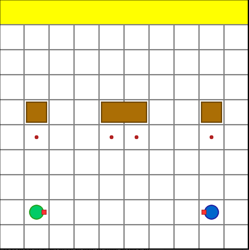
(b) (b) 10x10

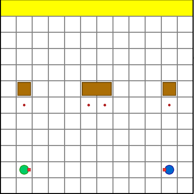
(c) (c) 12x12

Figure 10: Experimental environments.

Goal. The objective of the two robots is to learn collaboratively push the middle big box to the goal area at the top rather than pushing a small box on each own.

State. The global state information consists of the position and orientation of each robot and each box’s position in a grid world.

Primitive-Action Space. move forward, turn-left, turn-right and stay.

Macro-Action Space.

$\bullet$ One-step macro-actions: Turn-left, Turn-right, and Stay.

$\bullet$ Multi-step macro-actions: Move-to-small-box(i) that navigates the robot to the red spot below the corresponding small box and terminate with robot facing the box; Move-to-big-box(i) that navigates the robot to a red spot below the big box and terminate with robot facing the big box; Push that operates the robot to keep moving forward and terminate while arriving the world’s boundary, touching the big box along or pushing a small box to the goal.

Observation Space. In both the primitive-observation and macro-observation, each robot is only allowed to capture one of five states of the cell in front of it: empty, teammate, boundary, small box, big box.

Dynamics. The transition in this task is deterministic. Boxes can only be moved towards the north when the robot faces the box and moves forward. The small box can be moved by a single robot while the big box require two robots to move it together.

Rewards. The team receives $+300$ for pushing big box to the goal area and $+20$ for pushing a small box to the goal area. A penalty $-10$ is issued when any robot hits the boundary or pushes the big box on its own.

Episode Termination. Each episode terminates when any box is pushed to the goal area, or when 100 timesteps has elapsed.

Results.

(a)

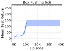
(b)

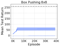
(c)

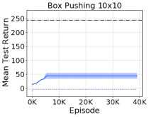
(d)

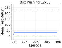
(e)

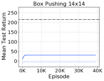
(f)

Figure 11: Decentralized learning with macro-actions vs primitive-actions.

(a)

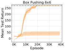
(b)

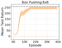
(c)

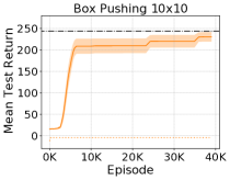
(d)

(e)

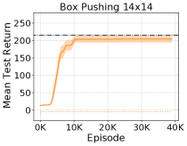
(f)

Figure 12: Centralized learning with macro-actions vs primitive-actions.

(a)

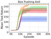
(b)

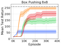
(c)

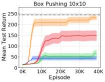
(d)

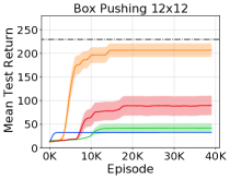
(e)

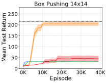
(f)

Figure 13: Comparison of macro-action-based multi-agent actor-critic methods.

(a)

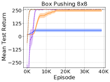
(b)

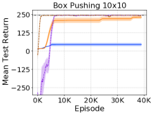
(c)

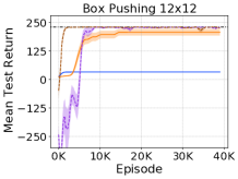
(d)

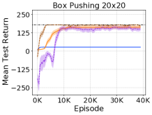
(e)

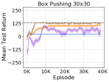
(f)

Figure 14: Comparison of macro-action-based actor-critic methods and value-based methods

D.2 Overcooked

(a) (a) Overcooked-A

(b) (b) Overcooked-B

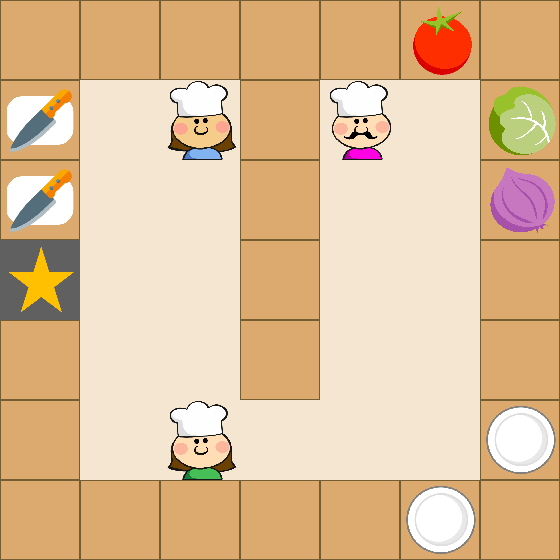
(c) (c) Overcooked-C

(d) (d) Lettuce-Onion-Tomato salad recipe

Figure 15: Experimental environments.

Goal. Three agents need to learn cooperating with each other to prepare a Tomato-Lettuce-Onion salad and deliver it to the ‘star’ counter cell as soon as possible. The challenge is that the recipe of making a tomato-lettuce-onion salad is unknown to agents. Agents have to learn the correct procedure in terms of picking up raw vegetables, chopping, and merging in a plate before delivering.

State Space. The environment is a 7×7 grid world involving three agents, one tomato, one lettuce, one onion, two plates, two cutting boards and one delivery cell. The global state information consists of the positions of each agent and above items, and the status of each vegetable: chopped, unchopped, or the progress under chopping.

Primitive-Action Space. Each agent has five primitive-actions: up, down, left, right and stay. Agents can move around and achieve picking, placing, chopping and delivering by standing next to the corresponding cell and moving against it (e.g., in Fig. 15a, the pink agent can move right and then move up to pick up the tomato).

Macro-Action Space. Here, we first describe the main function of each macro-action and then list the corresponding termination conditions.

• Five one-step macro-actions that are the same as the primitive ones;

• Chop, cuts a raw vegetable into pieces (taking three time steps) when the agent stands next to a cutting board and an unchopped vegetable is on the board, otherwise it does nothing; and it terminates when:

  • The vegetable on the cutting board has been chopped into pieces;

  • The agent is not next to a cutting board;

  • There is no unchopped vegetable on the cutting board;

  • The agent holds something in hand.

• Get-Lettuce, Get-Tomato, and Get-Onion, navigate the agent to the latest observed position of the vegetable, and pick the vegetable up if it is there; otherwise, the agent moves to check the initial position of the vegetable. The corresponding termination conditions are listed below:

  • The agent successfully picks up a chopped or unchopped vegetable;

  • The agent observes the target vegetable is held by another agent or itself;

  • The agent is holding something else in hand;

  • The agent’s path to the vegetable is blocked by another agent;

  • The agent does not find the vegetable either at the latest observed location or the initial location;

  • The agent attempts to enter the same cell with another agent, but has a lower priority than another agent.

• Get-Plate-1/2, navigates the agent to the latest observed position of the plate, and picks the vegetable up if it is there; otherwise, the agent moves to check the initial position of the vegetable. The corresponding termination conditions are listed below:

  • The agent successfully picks up a plate;

  • The agent observes the target plate is held by another agent or itself;

  • The agent is holding something else in hand;

  • The agent’s path to the plate is blocked by another agent;

  • The agent does not find the plate either at the latest observed location or at the initial location;

  • The agent attempts to enter the same cell with another agent but has a lower priority than another agent.

• Go-Cut-Board-1/2, navigates the agent to the corresponding cutting board with the following termination conditions:

  • The agent stops in front of the corresponding cutting board, and places an in-hand item on it if the cutting board is not occupied;

  • If any other agent is using the target cutting board, the agent stops next to the teammate;

  • The agent attempts to enter the same cell with another agent but has a lower priority than another agent.

• Go-Counter (only available in Overcook-B, Fig. 1(c)), navigates the agent to the center cell in the middle of the map when the cell is not occupied, otherwise it moves to an adjacent cell. If the agent is holding an object the object will be placed. If an object is in the cell, the object will be picked up.

• Deliver, navigates the agent to the ‘star’ cell for delivering with several possible termination conditions:

  • The agent places the in-hand item on the cell if it is holding any item;

  • If any other agent is standing in front of the ‘star’ cell, the agent stops next to the teammate;

  • The agent attempts to enter the same cell with another agent, but has a lower priority than another agent.

Observation Space: The macro-observation space for each agent is the same as the primitive observation space. Agents are only allowed to observe the positions and status of the entities within a $5\times 5$ view centered on the agent. The initial position of all the items are known to agents.

Dynamics: The transition in this task is deterministic. If an agent delivers any wrong item, the item will be reset to its initial position. From the low-level perspective, to chop a vegetable into pieces on a cutting board, the agent needs to stand next to the cutting board and executes left three times. Only the chopped vegetable can be put on a plate.

Reward: $+10$ for chopping a vegetable, $+200$ terminal reward for delivering a tomato-lettuce-onion salad, $-5$ for delivering any wrong entity, and $-0.1$ for every timestep.

Episode Termination: Each episode terminates either when agents successfully deliver a tomato-lettuce-onion salad or reaching the maximal time steps, 200.

Results

(a)

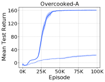
(b)

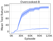
(c)

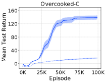
(d)

Figure 16: Decentralized learning with macro-actions vs primitive-actions.

(a)

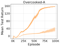
(b)

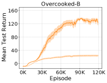
(c)

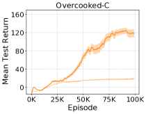
(d)

Figure 17: Centralized learning with macro-actions vs primitive-actions.

(a)

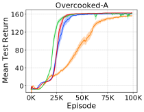
(b)

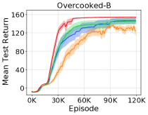
(c)

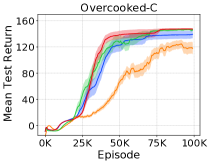
(d)

Figure 18: Comparison of macro-action-based multi-agent actor-critic methods.

(a)

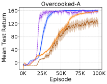
(b)

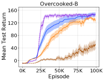
(c)

Figure 19: Comparisons of macro-action-based actor-critic methods and value-based methods.

D.3 Warehouse Tool Delivery

(a) (a) Warehouse-A

(b) (b) Warehouse-B

(c) (c) Warehouse-C

(d) (d) Warehouse-D

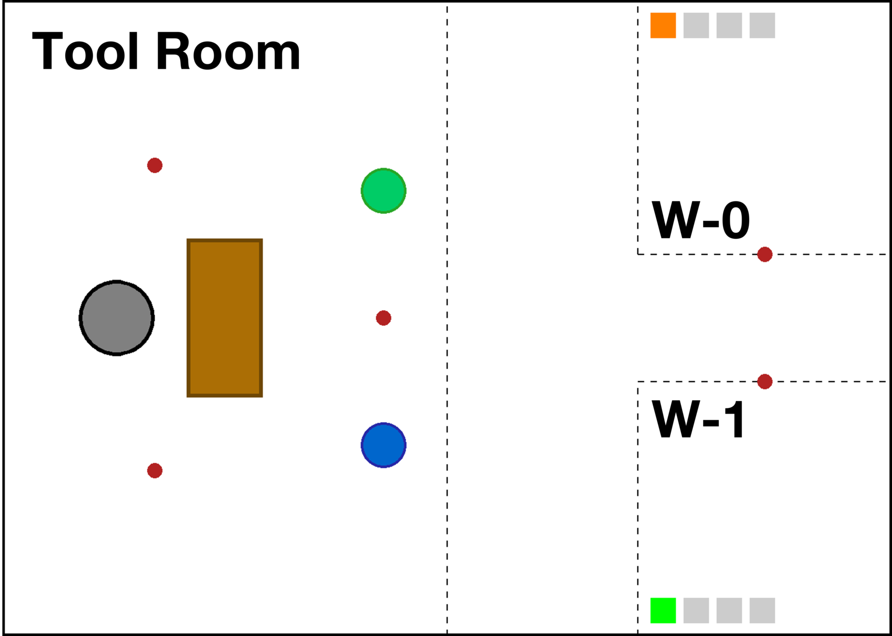
(e) (e) Warehouse-E

Figure 20: Experimental environments.

In this Warehouse Tool Delivery domain, we consider five different scenarios shown in Fig. 20. To further examine the scalability of our methods and the effectiveness of Mac-IAICC on handling more noisy asynchronous terminations over robots, we consider many variants in terms of both the number of robots and the number of humans as well as having faster human(orange) in the environment.

Goal. Under all scenarios, in each workshop, a human is working on an assembly task involving 4 subtasks to be finished (each subtask takes amount of primitive time steps). At the beginning, each human has already got the tool for the first subtask and immediately starts. In order to continue, the human needs a particular tool for each following subtask. In the scenarios, humans either work in the same speed (Fig. 20a, 20b, 20d) or have one of them working faster (the orange one in Fig.20c and 20e). A team of robots includes a robot arm (gray) with the duty of finding tools for each human on the table (brown) and passing them to mobile robots (green, blue and yellow) who are responsible for delivering tools to the humans. The objective of the robots is to assist the humans to finish their assembly tasks as soon as possible by finding and delivering the correct tools in the proper order. To make this problem more challenging, the correct tools needed by each human are unknown to robots, which has to be learned during training in order to perform timely delivery without letting humans wait.

State. The environment is either a $5\times 7$ (Fig. 20a and  20e) or a $5\times 9$ (Fig. 20b - 20d) continuous space. A global state consists of the 2D position of each mobile robots, the execution status of the arm robot’s current macro-action (e.g how munch steps are left for completing the macro-action, but in real-world, this should be the angle and speed of each arm’s joint), the subtask each human is working with a percentage indicating the progress of the subtask, and the position of each tools (either on the brown table or carried by a mobile robot). The initial state of every episode is deterministic as shown in Fig. 20, where humans always start from the first step.

Macro-Action Space.

The available macro-actions for each mobile robot include:

$\bullet$ Go-W(i), navigates to the red waypoint at the corresponding workshop;

$\bullet$ Go-TR, navigates to the red waypoint (covered by the blue robot in Fig. 20c and 20d) at the right side of the tool room;

$\bullet$ Get-Tool, navigates to a pre-allocated waypoint besides the arm robot and waits over there until either 10 timesteps have passed or receiving a tool from the gray robot.

The available macro-actions for the arm robot include:

$\bullet$ Search-Tool(i), takes 6 timesteps to find tool $i$ and place it in a staging area (containing at most two tools) when the area is not fully occupied, otherwise freezes the robot for the same amount of time;

$\bullet$ Pass-to-M(i), takes 4 timesteps to pass the first found tool to a mobile robot from the staging area;

$\bullet$ Wait-M, takes 1 timestep to wait for mobile robots coming.

Macro-Observation Space.

The arm robot’s macro-observation include the information about the type of each tool in the staging area and which mobile robot is waiting beside.

Each mobile robot always observes its own position and the type of each tool carried by itself, while observes the number of tools in the staging area or the subtask a human working on only when locating at the tool room or the workshop respectively.

Dynamics. Transitions are deterministic. Each mobile robot moves in a fixed velocity 0.8 and is only allowed to receive tools from the arm robot rather than from humans. Note that each human is only allowed to possess the tool for the next subtask from a mobile robot when the robot locates at the corresponding workshop and carries the correct tool. Humans are not allowed to pass tool back to mobile robots. There are enough tools for humans on the table in tool room, such that the number of each type of tool exactly matches with the number of humans in the environment. Human cannot start the next subtask without obtaining the correct tool. Humans’ dynamics on their tasks are shown in Table 1.

Table 1: The number of time steps taken by each human on each subtask in scenarios.

Scenarios	Warehouse-A	Warehouse-B	Warehouse-C	Warehouse-D	Warehouse-E
Human-0	$[27,20,20,20]$	$[40,40,40,40]$	$[38,38,38,38]$	$[40,40,40,40]$	$[18,15,15,15]$
Human-1	$[27,20,20,20]$	$[40,40,40,40]$	$[38,38,38,38]$	$[40,40,40,40]$	$[48,18,15,15]$
Human-2	N/A	$[40,40,40,40]$	$[27,27,27,27]$	$[40,40,40,40]$	N/A
Human-3	N/A	N/A	N/A	$[40,40,40,40]$	N/A

Rewards. The team receives a $+100$ reward when a correct tool is delivered to a human in time while getting an extra $-20$ penalty for a delayed delivery such that the human has paused over there. A $-10$ reward occurs when the gray robot does Pass-to-M(i) but the mobile robot $i$ is not next to it, and a $-1$ reward is issued every time step.

Episode Termination. Each episode terminates when all humans obtained all the correct tools for all subtasks, otherwise, the episode will run until the maximal time steps (200 for Warehouse-A and E, 250 for Warehouse-B and C, 300 for Warehous-D).

Results

(a)

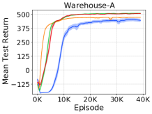
(b)

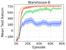
(c)

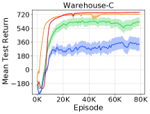
(d)

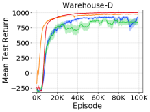
(e)

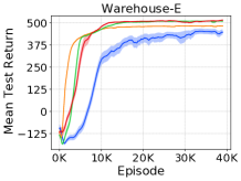
(f)

Figure 21: Comparison of macro-action-based multi-agent actor-critic methods.

Ablation Study

Figure 22: Results of an ablation study.

Scenarios	Ablation Experiment
Human-0	$[18,18,18,18]$
Human-1	$[18,18,18,18]$
Human-2	N/A
Human-3	N/A

Table 2: The number of time steps taken by each human in the ablation study.

We also conducted an ablation experiment in Warehouse-A, where two humans still operate at the same speed on their tasks but faster than the original setting. Such a change makes agents’ learning more difficult, because the probability of having a delayed delivery for each tool grows, especially when agents are exploring. Agents likely receives more penalty during training. Fig. 22 shows the learning quality of Naive Mac-IACC degrades markedly and becomes much less stable with higher variance than its performance in the original domain configuration (shown in Fig. 21). In contrast, Mac-IAICC remains its high-quality performance, which reveals its robustness to noisy penalty signals and further proves the advantage of separately training a centralized critic depending on each agent’s own macro-action terminations. Both Mac-CAC and Mac-IAC still cannot rival Mac-IAICC.

(a)

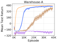
(b)

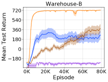
(c)

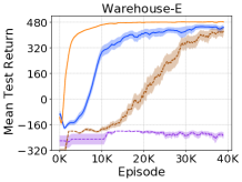
(d)

Figure 23: Comparison of macro-action-based actor-critic methods and value-based methods.

Appendix E Training Details

Our results are generated by running on a cluster of computer nodes under "CentOS Linux" operating system. We use the CPUs including "Dual Intel Xeon E5-2650", "Dual Intel Xeon E5-2680 v2", "Dual Intel Xeon E5-2690 v3".

E.1 Network Architecture

For all domains, all methods apply the same neural network architecture for both actor & critic network and Q-network. Each of them consists of two fully connected (FC) layers with Leaky-Relu activation function, one GRU layer [Cho et al., 2014] and one more FC layer followed by an output layer. The number of neurons in each layer for Decentralized(Dec) or Centralized(Cen) actor, critic or Q-network are shown in Table 3. Empirical experiments show that centralized actor and critic usually need more neurons to deal with larger joint macro-observation and macro-action spaces.

Table 3: Number of neurons on each layer in networks for all methods in domains

Domain	Box Pushing		Overcooked		Warehouse
Actor & Critic & Q-network	Dec	Cen	Dec	Cen	Dec	Cen
MLP-1	32	32	32	128	32	32
MLP-2	32	32	32	128	32	32
GRU	32	64	32	64	32	64
MLP-3	32	32	32	64	32	32

E.2 Hyper-Parameters for macro-action-based actor-critic methods

In following subsections, we first list the hyper-parameter candidates used for tuning each method via grid search in the corresponding domain, and then show the hyper-parameter table with the parameters used by each method achieving the best performance. We choose the best performance of each method depending on its final converged value as the first priority and the sample efficiency as the second.

$\bullet$ Box Pushing:

Table 4: Hyper-parameter candidates for grid search tuning.

Learning rate pair (actor,critic)	(1e-3,3e-3), (1e-3,1e-3) (5e-4,3e-3), (5e-4,1e-3)
	(5e-4,5e-4), (3e-4,3e-3)
Episodes per train	8, 16, 32
Target-net update freq (episode)	32, 64, 128
N-step TD	0, 3, 5

Table 5: Hyper-parameter candidates for grid search tuning.

Learning rate pair (actor,critic)	(1e-3,3e-3), (1e-3,1e-3) (5e-4,3e-3), (5e-4,1e-3)
	(5e-4,5e-4), (3e-4,3e-3)
Episodes per train	48
Target-net update freq (episode)	48, 96, 144
N-step TD	0, 3, 5

Table 6: Hyper-parameters used for methods in Box Pushing $6\times 6$.

Parameter	IAC	CAC	Mac-IAC	Mac-CAC	Mac-NIACC	Mac-IAICC
Training Episodes	40K	40K	40K	40K	40K	40K
Actor Learning rate	0.001	0.0005	0.0005	0.0003	0.0005	0.0003
Critic Learning rate	0.003	0.0005	0.001	0.003	0.001	0.003
Episodes per train	8	8	48	48	48	48
Target-net update freq	32	64	48	144	144	96
(episode)
N-step TD	5	5	5	5	0	0
$\epsilon_{\text{start}}$	1	1	1	1	1	1
$\epsilon_{\text{end}}$	0.01	0.01	0.01	0.01	0.01	0.01
$\epsilon_{\text{decay}}$ (episode)	4K	4K	4K	4K	4K	4K

Table 7: Hyper-parameters used for methods in Box Pushing $8\times 8$.

Parameter	IAC	CAC	Mac-IAC	Mac-CAC	Mac-NIACC	Mac-IAICC
Training Episodes	40K	40K	40K	40K	40K	40K
Actor Learning rate	0.001	0.001	0.001	0.0005	0.0005	0.0003
Critic Learning rate	0.003	0.003	0.003	0.003	0.001	0.003
Episodes per train	8	8	16	48	48	48
Target-net update freq	32	32	32	48	144	144
(episode)
N-step TD	3	0	5	3	0	0
$\epsilon_{\text{start}}$	1	1	1	1	1	1
$\epsilon_{\text{end}}$	0.01	0.01	0.01	0.01	0.01	0.01
$\epsilon_{\text{decay}}$ (episode)	4K	4K	4K	4K	4K	4K

Table 8: Hyper-parameters used for methods in Box Pushing $10\times 10$.

Parameter	IAC	CAC	Mac-IAC	Mac-CAC	Mac-NIACC	Mac-IAICC
Training Episodes	40K	40K	40K	40K	40K	40K
Actor Learning rate	0.001	0.001	0.001	0.001	0.0005	0.0003
Critic Learning rate	0.003	0.003	0.001	0.003	0.001	0.003
Episodes per train	8	8	32	48	48	32
Target-net update freq	64	32	32	96	144	64
(episode)
N-step TD	0	0	5	3	0	0
$\epsilon_{\text{start}}$	1	1	1	1	1	1
$\epsilon_{\text{end}}$	0.01	0.01	0.01	0.01	0.01	0.01
$\epsilon_{\text{decay}}$ (episode)	6K	6K	6K	6K	6K	6K

Table 9: Hyper-parameters used for methods in Box Pushing $12\times 12$.

Parameter	IAC	CAC	Mac-IAC	Mac-CAC	Mac-NIACC	Mac-IAICC
Training Episodes	40K	40K	40K	40K	40K	40K
Actor Learning rate	0.001	0.001	0.001	0.0005	0.0005	0.0003
Critic Learning rate	0.003	0.003	0.003	0.0005	0.001	0.003
Episodes per train	8	8	8	32	48	32
Target-net update freq	128	128	64	64	96	128
(episode)
N-step TD	0	0	5	3	0	0
$\epsilon_{\text{start}}$	1	1	1	1	1	1
$\epsilon_{\text{end}}$	0.01	0.01	0.01	0.01	0.01	0.01
$\epsilon_{\text{decay}}$ (episode)	6K	6K	6K	6K	6K	6K

Table 10: Hyper-parameters used for methods in Box Pushing $14\times 14$.

Parameter	IAC	CAC	Mac-IAC	Mac-CAC	Mac-NIACC	Mac-IAICC
Training Episodes	40K	40K	40K	40K	40K	40K
Actor Learning rate	0.001	0.001	0.001	0.001	0.001	0.0003
Critic Learning rate	0.003	0.003	0.003	0.001	0.003	0.003
Episodes per train	8	8	8	48	16	32
Target-net update freq	128	64	32	96	32	64
(episode)
N-step TD	0	0	3	3	5	0
$\epsilon_{\text{start}}$	1	1	1	1	1	1
$\epsilon_{\text{end}}$	0.01	0.01	0.01	0.01	0.01	0.01
$\epsilon_{\text{decay}}$ (episode)	8K	8K	8K	8K	8K	8K

$\bullet$ Overcooked:

Table 11: Hyper-parameter candidates for grid search tuning.

Learning rate pair (actor,critic)	(1e-4, 3e-3) (3e-4,3e-3)
Episodes per train	4
Target-net update freq (episode)	8, 16, 32
N-step TD	3, 5

Table 12: Hyper-parameter candidates for grid search tuning.

Learning rate pair (actor,critic)	(1e-4, 3e-3) (3e-4,3e-3)
Episodes per train	8, 16
Target-net update freq (episode)	16, 32, 64
N-step TD	3, 5

Table 13: Hyper-parameters used for methods in Overcooked-A.

Parameter	IAC	CAC	Mac-IAC	Mac-CAC	Mac-NIACC	Mac-IAICC
Training Episodes	100K	100K	100K	100K	100K	100K
Actor Learning rate	0.0003	0.0003	0.0003	0.0001	0.0003	0.0003
Critic Learning rate	0.003	0.003	0.003	0.003	0.003	0.003
Episodes per train	4	8	4	8	4	8
Target-net update freq	8	16	8	32	16	32
(episode)
N-step TD	5	5	5	5	5	5
$\epsilon_{\text{start}}$	1	1	1	1	1	1
$\epsilon_{\text{end}}$	0.05	0.05	0.05	0.05	0.05	0.05
$\epsilon_{\text{decay}}$ (episode)	20K	20K	20K	20K	20K	20K

Table 14: Hyper-parameters used for methods in Overcooked-B.

Parameter	IAC	CAC	Mac-IAC	Mac-CAC	Mac-NIACC	Mac-IAICC
Training Episodes	120K	120K	120K	120K	120K	120K
Actor Learning rate	0.0003	0.0003	0.0003	0.0001	0.0003	0.0003
Critic Learning rate	0.003	0.003	0.003	0.003	0.003	0.003
Episodes per train	4	4	4	4	8	4
Target-net update freq	8	16	8	16	16	32
(episode)
N-step TD	5	5	5	3	5	5
$\epsilon_{\text{start}}$	1	1	1	1	1	1
$\epsilon_{\text{end}}$	0.05	0.05	0.05	0.05	0.05	0.05
$\epsilon_{\text{decay}}$ (episode)	20K	20K	20K	20K	20K	20K

Table 15: Hyper-parameters used for methods in Overcooked-C.

Parameter	IAC	CAC	Mac-IAC	Mac-CAC	Mac-NIACC	Mac-IAICC
Training Episodes	100K	100K	100K	100K	100K	100K
Actor Learning rate	0.0003	0.0003	0.0003	0.0001	0.0003	0.0003
Critic Learning rate	0.003	0.003	0.003	0.003	0.003	0.003
Episodes per train	8	8	8	8	8	8
Target-net update freq	32	32	32	32	16	32
(episode)
N-step TD	5	5	5	3	5	5
$\epsilon_{\text{start}}$	1	1	1	1	1	1
$\epsilon_{\text{end}}$	0.05	0.05	0.05	0.05	0.05	0.05
$\epsilon_{\text{decay}}$ (episode)	20K	20K	20K	20K	20K	20K

$\bullet$ Warehouse Tool Delivery:

Table 16: Hyper-parameter candidates for grid search tuning.

Learning rate pair (actor,critic)	(1e-3,1e-3), (5e-4,1e-3) (5e-4,5e-4) (3e-4,3e-3)
Episodes per train	4, 8
Target-net update freq (episode)	8, 16, 32, 64
N-step TD	0, 3, 5

Table 17: Hyper-parameter candidates for grid search tuning.

Learning rate pair (actor,critic)	(1e-3,1e-3), (5e-4,1e-3) (5e-4,5e-4) (3e-4,3e-3)
Episodes per train	16
Target-net update freq (episode)	16, 32, 64
N-step TD	0, 3, 5

Table 18: Hyper-parameters used for methods in Warehouse-A.

Parameter	Mac-IAC	Mac-CAC	Mac-NIACC	Mac-IAICC
Training Episodes	40K	40K	40K	40K
Actor Learning rate	0.0003	0.0003	0.0003	0.0005
Critic Learning rate	0.003	0.003	0.003	0.0005
Episodes per train	4	4	4	4
Target-net update freq	32	32	32	32
(episode)
N-step TD	5	5	3	5
$\epsilon_{\text{start}}$	1	1	1	1
$\epsilon_{\text{end}}$	0.01	0.01	0.01	0.01
$\epsilon_{\text{decay}}$ (episode)	10K	10K	10K	10K

Table 19: Hyper-parameters used for methods in Warehouse-A for ablation.

Parameter	Mac-IAC	Mac-CAC	Mac-NIACC	Mac-IAICC
Training Episodes	40K	40K	40K	40K
Actor Learning rate	0.0005	0.0005	0.0003	0.0005
Critic Learning rate	0.0005	0.001	0.003	0.0005
Episodes per train	16	8	8	4
Target-net update freq	16	64	64	64
(episode)
N-step TD	5	5	5	5
$\epsilon_{\text{start}}$	1	1	1	1
$\epsilon_{\text{end}}$	0.05	0.05	0.05	0.05
$\epsilon_{\text{decay}}$ (episode)	10K	10K	10K	10K

Table 20: Hyper-parameters used for methods in Warehouse-B.

Parameter	Mac-IAC	Mac-CAC	Mac-NIACC	Mac-IAICC
Training Episodes	40K	40K	40K	40K
Actor Learning rate	0.0005	0.0005	0.0003	0.0003
Critic Learning rate	0.0005	0.001	0.003	0.003
Episodes per train	8	4	16	4
Target-net update freq	64	64	64	32
(episode)
N-step TD	5	5	5	5
$\epsilon_{\text{start}}$	1	1	1	1
$\epsilon_{\text{end}}$	0.01	0.01	0.01	0.01
$\epsilon_{\text{decay}}$ (episode)	10K	10K	10K	10K

Table 21: Hyper-parameters used for methods in Warehouse-C.

Parameter	Mac-IAC	Mac-CAC	Mac-NIACC	Mac-IAICC
Training Episodes	80K	80K	80K	80K
Actor Learning rate	0.0005	0.0003	0.0003	0.0003
Critic Learning rate	0.001	0.003	0.003	0.003
Episodes per train	8	8	8	8
Target-net update freq	64	64	64	64
(episode)
N-step TD	5	5	5	5
$\epsilon_{\text{start}}$	1	1	1	1
$\epsilon_{\text{end}}$	0.01	0.01	0.01	0.01
$\epsilon_{\text{decay}}$ (episode)	10K	10K	10K	10K

Table 22: Hyper-parameters used for methods in Warehouse-D.

Parameter	Mac-IAC	Mac-CAC	Mac-NIACC	Mac-IAICC
Training Episodes	80K	80K	80K	80K
Actor Learning rate	0.0003	0.0003	0.0005	0.0003
Critic Learning rate	0.003	0.003	0.005	0.003
Episodes per train	4	8	4	8
Target-net update freq	16	64	32	64
(episode)
N-step TD	5	5	5	5
$\epsilon_{\text{start}}$	1	1	1	1
$\epsilon_{\text{end}}$	0.01	0.01	0.01	0.01
$\epsilon_{\text{decay}}$ (episode)	10K	10K	10K	10K

Table 23: Hyper-parameters used for methods in Warehouse-E.

Parameter	Mac-IAC	Mac-CAC	Mac-NIACC	Mac-IAICC
Training Episodes	100K	100K	100K	100K
Actor Learning rate	0.0005	0.0003	0.0003	0.0005
Critic Learning rate	0.001	0.003	0.003	0.0005
Episodes per train	4	4	4	4
Target-net update freq	32	16	32	32
(episode)
N-step TD	5	5	5	5
$\epsilon_{\text{start}}$	1	1	1	1
$\epsilon_{\text{end}}$	0.05	0.05	0.05	0.05
$\epsilon_{\text{decay}}$ (episode)	10K	10K	10K	10K

E.3 Hyper-Parameters for macro-action-based value-based methods

$\bullet$ Box Pushing:

Table 24: Hyper-parameter candidates for grid search tuning.

Learning rate	5e-4, 1e-3
batch size	32, 64, 128

Table 25: Hyper-parameters used in Box Pushing $8\times 8$.

Parameter	Mac-Dec-Q	Mac-Cen-Q
Training Episodes	40K	40K
Learning rate	0.001	0.001
Batch size	64	64
Replay-buffer size (step)	100K	100K
Train freq (step)	10	10
Trace length	10	10
Target-net update freq (step)	5K	5K
$\epsilon_{\text{start}}$	1	1
$\epsilon_{\text{end}}$	0.05	0.05
$\epsilon_{\text{decay}}$ (episode)	4K	4K

Table 26: Hyper-parameters used in Box Pushing $10\times 10$.

Parameter	Mac-Dec-Q	Mac-Cen-Q
Training Episodes	40K	40K
Learning rate	0.001	0.001
Batch size	32	128
Replay-buffer size (step)	100K	100K
Train freq (step)	14	14
Trace length	14	14
Target-net update freq (step)	5K	5K
$\epsilon_{\text{start}}$	1	1
$\epsilon_{\text{end}}$	0.05	0.05
$\epsilon_{\text{decay}}$ (episode)	6K	6K

Table 27: Hyper-parameters used in Box Pushing $12\times 12$.

Parameter	Mac-Dec-Q	Mac-Cen-Q
Training Episodes	40K	40K
Learning rate	0.001	0.001
Batch size	32	128
Replay-buffer size (step)	100K	100K
Train freq (step)	20	20
Trace length	20	20
Target-net update freq (step)	5K	5K
$\epsilon_{\text{start}}$	1	1
$\epsilon_{\text{end}}$	0.05	0.05
$\epsilon_{\text{decay}}$ (episode)	6K	6K

Table 28: Hyper-parameters used in Box Pushing $20\times 20$.

Parameter	Mac-Dec-Q	Mac-Cen-Q
Training Episodes	40K	40K
Learning rate	0.001	0.001
Batch size	32	64
Replay-buffer size (step)	100K	100K
Train freq (step)	35	35
Trace length	35	35
Target-net update freq (step)	5K	5K
$\epsilon_{\text{start}}$	1	1
$\epsilon_{\text{end}}$	0.05	0.05
$\epsilon_{\text{decay}}$ (episode)	8K	8K

Table 29: Hyper-parameters used in Box Pushing $30\times 30$.

Parameter	Mac-Dec-Q	Mac-Cen-Q
Training Episodes	40K	40K
Learning rate	0.0005	0.001
Batch size	32	32
Replay-buffer size (step)	100K	100K
Train freq (step)	45	45
Trace length	45	45
Target-net update freq (step)	5K	5K
$\epsilon_{\text{start}}$	1	1
$\epsilon_{\text{end}}$	0.05	0.05
$\epsilon_{\text{decay}}$ (episode)	8K	8K

$\bullet$ Overcooked:

Table 30: Hyper-parameter candidates for grid search tuning.

Learning rate	3e-5, 5e-5, 1e-4, 3e-4, 5e-4
batch size	32, 64
Train freq (step)	64, 128
Replay-buffer size (episode)	500, 1K, 2K, 3K

Table 31: Hyper-parameters used in Overcooked-A.

Parameter	Mac-Dec-Q	Mac-Cen-Q
Training Episodes	100K	100K
Learning rate	0.0005	0.00003
Batch size	64	64
Replay-buffer size (episode)	1K	1K
Train freq (step)	64	64
Target-net update freq (step)	5K	5K
$\epsilon_{\text{start}}$	1	1
$\epsilon_{\text{end}}$	0.05	0.05
$\epsilon_{\text{decay}}$ (episode)	20K	20K

Table 32: Hyper-parameters used in Overcooked-B.

Parameter	Mac-Dec-Q	Mac-Cen-Q
Training Episodes	100K	100K
Learning rate	0.0005	0.0001
Batch size	32	32
Replay-buffer size (episode)	3K	500
Train freq (step)	64	64
Target-net update freq (step)	5K	5K
$\epsilon_{\text{start}}$	1	1
$\epsilon_{\text{end}}$	0.05	0.05
$\epsilon_{\text{decay}}$ (episode)	20K	20K

$\bullet$ Warehouse Tool Delivery:

Table 33: Hyper-parameter candidates for grid search tuning.

Learning rate	5e-5, 1e-4
batch size	32, 64
Train freq (step)	64, 128
Replay-buffer size (episode)	1K, 2K

Table 34: Hyper-parameters used in Warehouse-A.

Parameter	Mac-Dec-Q	Mac-Cen-Q
Training Episodes	40K	40K
Learning rate	0.0001	0.0001
Batch size	64	64
Replay-buffer size (episode)	2K	2K
Train freq (step)	128	128
Target-net update freq (step)	5K	5K
$\epsilon_{\text{start}}$	1	1
$\epsilon_{\text{end}}$	0.05	0.05
$\epsilon_{\text{decay}}$ (episode)	10K	10K

Table 35: Hyper-parameters used in Warehouse-B.

Parameter	Mac-Dec-Q	Mac-Cen-Q
Training Episodes	40K	40K
Learning rate	0.00005	0.00005
Batch size	64	64
Replay-buffer size (episode)	2K	2K
Train freq (step)	128	128
Target-net update freq (step)	5K	5K
$\epsilon_{\text{start}}$	1	1
$\epsilon_{\text{end}}$	0.05	0.05
$\epsilon_{\text{decay}}$ (episode)	10K	10K

Table 36: Hyper-parameters used in Warehouse-E.

Parameter	Mac-Dec-Q	Mac-Cen-Q
Training Episodes	100K	100K
Learning rate	0.0001	0.0001
Batch size	64	64
Replay-buffer size (episode)	2K	2K
Train freq (step)	128	128
Target-net update freq (step)	5K	5K
$\epsilon_{\text{start}}$	1	1
$\epsilon_{\text{end}}$	0.05	0.05
$\epsilon_{\text{decay}}$ (episode)	10K	10K

Appendix F Hardware Experiments

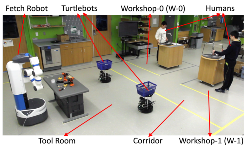
Figure 24: Overview of Warehouse-A hardware domain.

While simulation results validate that the proposed Mac-IAICC approach achieves the best performance for learning decentralized policies in various macro-action-based domains, we also extend scenario A of the Warehouse Tool Delivery task to a hardware domain. Fig. 24 provides an overview of the real-world experimental setup. An open area is divided into regions, a tool room, a corridor, and two workshops, to resemble the configuration shown in Fig. 1(e). This mission involves one Fetch Robot Wise et al. [2016] and two Turtlebots Koubaa et al. [2016] to cooperatively find and deliver three YCB tools Calli et al. [2015], in the order: a tape measure, a clamp and an electric drill, required by each human in order to assemble an IKEA table.

The Turtlebot’s navigation macro-actions were executed by using the ROS navigation stack Marder-Eppstein et al. [2010]. For Fetch’s manipulation macro-actions, we combined PCL bindings for Python Gualtieri et al. [2018], MoveIt Coleman et al. and the OpenRave simulator Diankov and Kuffner [2008] with an OMPL Şucan et al. [2012] plugin to achieve picking and placing of tools. The information about the number of tools in staging areas and each human’s working status was tracked and broadcast by ROS services but were only observable in the tool room and the corresponding workshop area respectively (to simulate possible visual information).

For the visualization of the real-robot experiment, please check the video in our supplementary.

Appendix G Behavior Visualization in Simulation

In this section, we display the decentralized behaviors learned by using Mac-IAICC under all considered domains.

G.1 Box Pushing

We show the behaviors learned under the grid world size $14\times 14$ in Fig. 25. Although the averaged performance of the training is not near-optimal (Fig. 13), several runs can learn the optimal behavior.

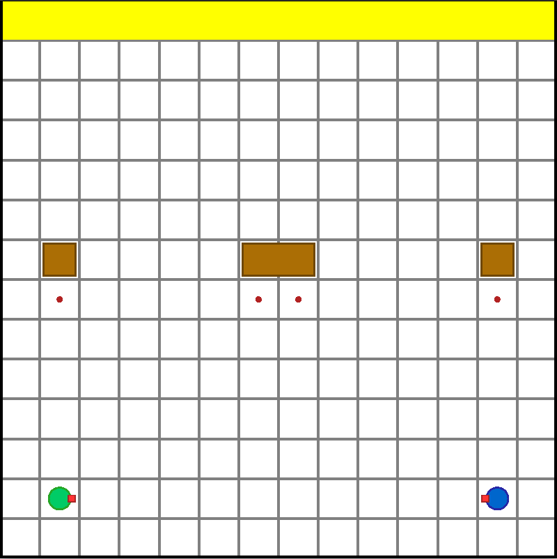
(a) (a) Green robot executes Move-to-big-box(1) to move to the left waypoint below the big box while the blue robot runs Move-to-big-box(2) to move to the right waypoint below the big box.

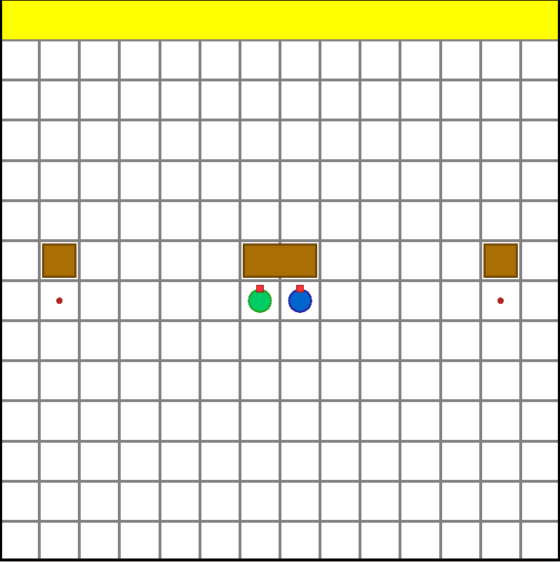
(b) (b) After completing the previous macro-actions, robots choose Push to move the big box towards the goal together.

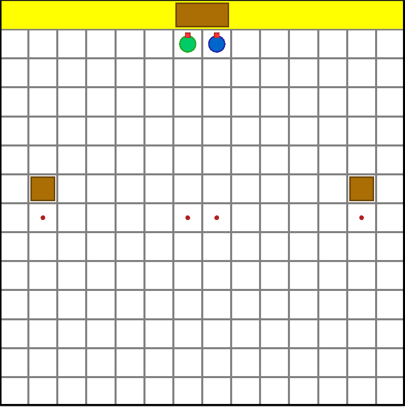
(c) (c) Robots finish the task by pushing the big box to the goal area.

Figure 25: Visualization of the optimal macro-action-based behaviors learned using Mac-IAICC in the Box Pushing domain under a $14\times 14$ grid world.

G.2 Overcooked

Map A: In this map, our method learns an efficient collaboration such as three agents separately get three different vegetables, and then go to the cutting board and chop them respectively. Especially, the pink agent leans to take away the chopped lettuce in order to make room for the incoming green agent to chop the onion (Fig. 27h - 27i). Details are shown below.

(a) (a) The blue agent executes Get-Lettuce. The pink agent executes Get-Tomato. The green agent executes Get-Onion.

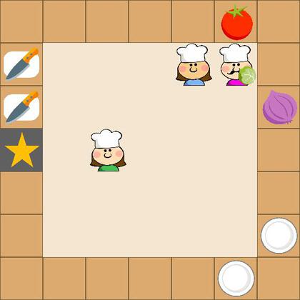
(b) (b) After getting the lettuce, the pink agent executes Go-Cut-Board-2.

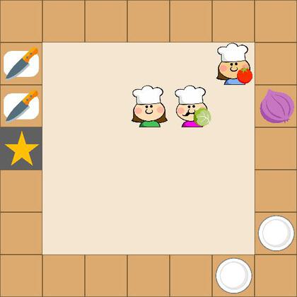
(c) (c) After getting the tomato, the blue agent executes Go-Cut-Board-1.

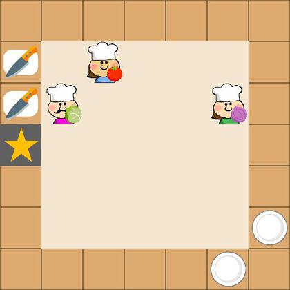
(d) (d) After getting the onion, the green agent executes Go-Cut-Board-2.

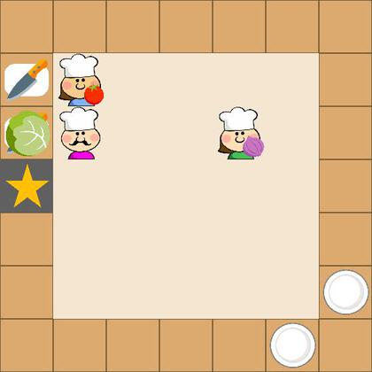
(e) (e) After placing the lettuce on the cutting board, the pink agent executes Chop.

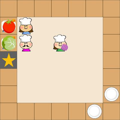
(f) (f) After placing the tomato on the cutting board, the blue agent executes Chop.

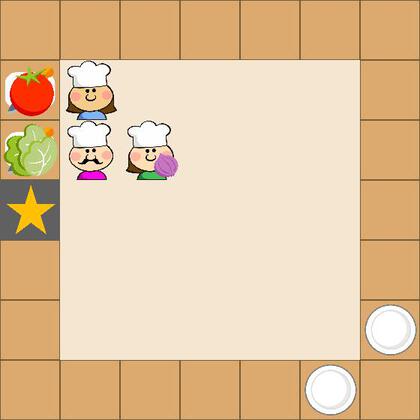
(g) (g) After finishing chopping the lettuce, the pink agent executes Get-Lettuce to pick it up.

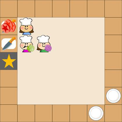
(h) (h) With the lettuce in hand, the pink agent executes Get-Plate-1.

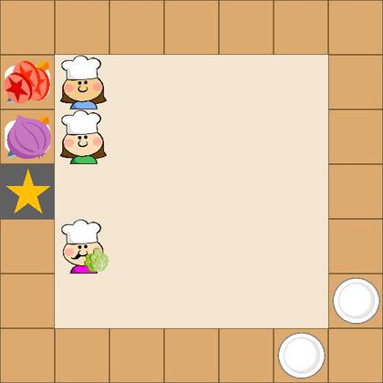
(i) (i) After placing the onion on the cutting board, the green agent executes Chop.

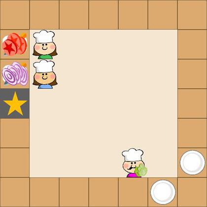
(j) (j) The green agent executes Get-Plate-2, and the blue agent keep running Move-Down to make room for the pink agent to merge the chopped vegetables later on.

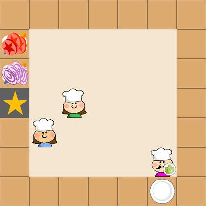
(k) (k) The pink agent reaches the plate and it is going to put the lettuce on the plate.

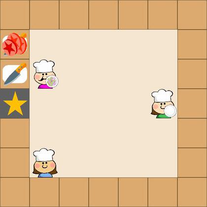
(l) (l) After putting the lettuce on the plate, the pink agent merges the onion in the plate by executing executes Get-Onion.

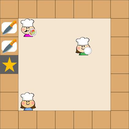
(a) (m) The pink agent gets the chopped tomato into the plate by executing Get-Tomato.

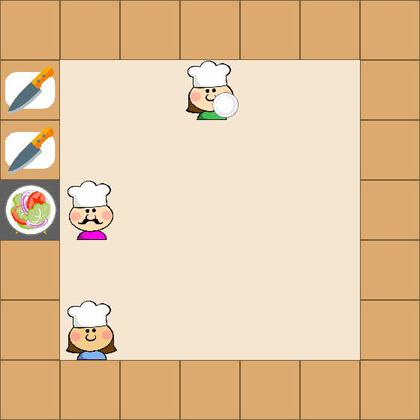
(b) (n) The pink agent successfully delivers the tomato-lettuce-onion salad by running Deliver.

Figure 27: Visualization of running decentralized policies learned by Mac-IAICC in Overcooked-A.

Map B: In this map, the decentralized policies trained by our method learns the collaboration such that the pink agent focuses on transporting items from right to left, while the other two agents cooperatively prepare the salad.

(a) (a) The blue agent executes Go-Cut-board-1. The green agent executes Go-Cut-board-2. The pink agent executes Get-Lettuce.

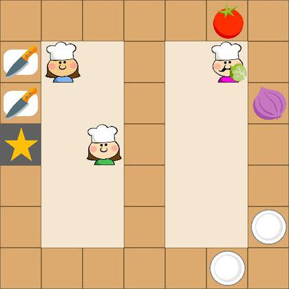
(b) (b) After getting the lettuce, the pink agent executes Go-Counter.

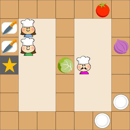
(c) (c) After putting the lettuce on the counter, the pink agent executes Get-Onion.

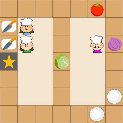
(d) (d) The green agent executes Get-Lettuce.

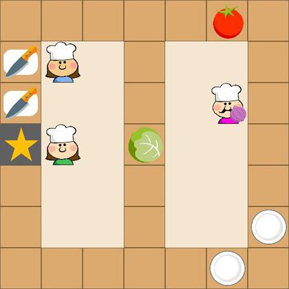
(e) (e) After getting the onion, the pink agent executes Go-Counter.

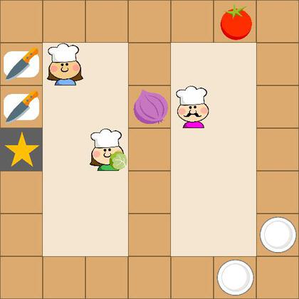
(f) (f) After getting the lettuce, the green agent executes Go-Cut-Board-2. Meanwhile the pink agent puts the onion on the counter, and then executes Get-Tomato. The blue agent executes Get-Onion.

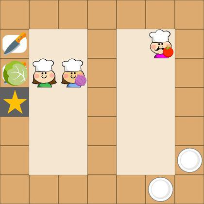
(g) (g) After putting the lettuce on the cutting board, the green executes Chop. Blue agent executes Go-Cut-Board-1 with onion in hand.

(h) (h) The blue agent executes Chop to cut the onion to pieces.

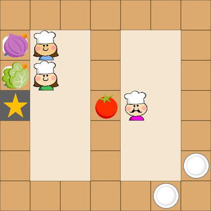
(a) (i) After putting the tomato on the counter, the pink agent executes Get-Plate-2. The green agent executes Get-Tomato.

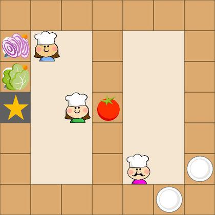
(b) (j) The blue agent finishes chopping the onion, and then picks it up by executing Get-Onion again.

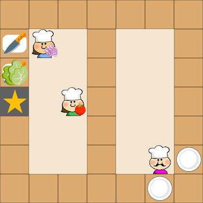
(c) (k) The blue agent keeps executing Moving-Down to make room for the green agent to chop tomato later on. Meanwhile the green agent moves towards the upper cutting board by executing Go-Cut-Board-1.

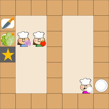
(d) (l) After getting the plate, the pink agent executes Go-Counter.

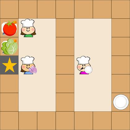
(e) (m) After putting the tomato on the cutting board, the green agent executes Chop.

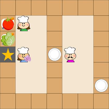
(f) (n) The pink agent puts the plate on the counter. The blue agent executes Go-Counter to get the plate.

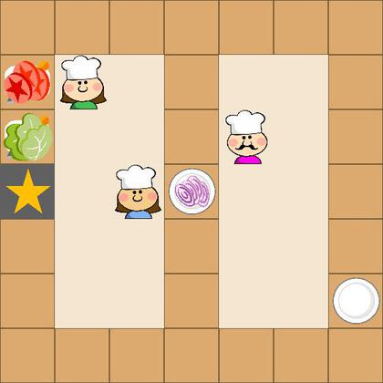
(g) (o) The green agent finishes chopping the tomato, while the blue agent puts chopped onion on the plate.

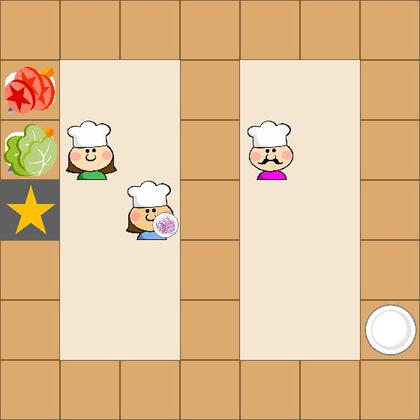
(h) (p) The green agent executes Go-Cut-Board-2 to make room for the blue agent to merge the tomato in to the plate.

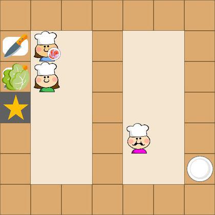
(i) (q) The blue agent executes Get-Lettuce. The green agent executes Go-Cut-Board-1.

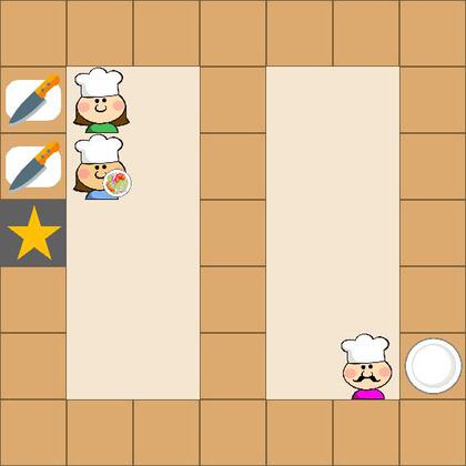
(j) (r) After putting the lettuce on the plate, the blue agent executes Deliver.

(k) (s) The blue agent successfully delivers the tomato-lettuce-onion salad.

Figure 29: Visualization of running decentralized policies learned by Mac-IAICC in Overcooked-B.

Map C: In this map, the best strategy is that the pink agent should take the advantage of the middle counters to pass vegetables to the other agent. Our method learns a sub-optimal policy such that the blue agent still crosses the narrow passage to get the vegetable at the right side of the map.

(a) (a) The blue agent executes Get-Lettuce. The pink agent executes Get-Onion. The green agent executes Get-Tomato.

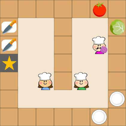
(b) (b) After getting the onion, the pink agent executes Go-Cut-Board-2.

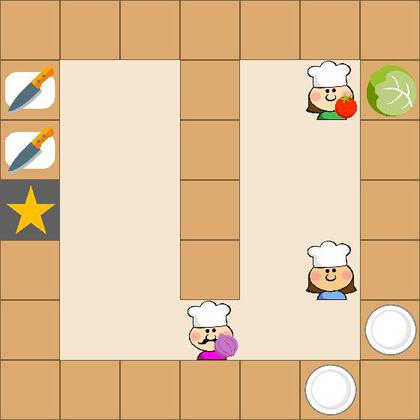
(c) (c) The green agent gets the tomato, and it executes Go-Cut-Board-2.

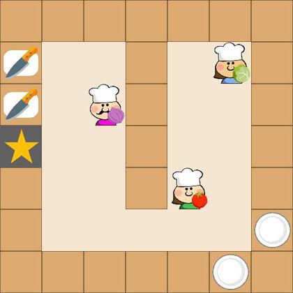
(d) (d) The blue agent gets the lettuce, and it executes Go-Cut-Board-1.

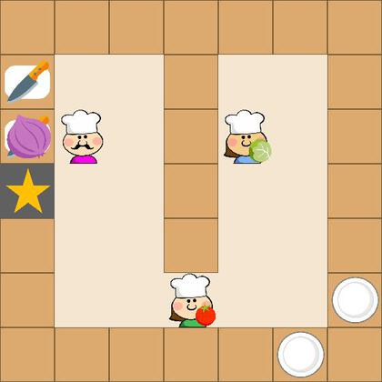
(e) (e) After putting the onion on the cutting board, the pink agent executes Chop.

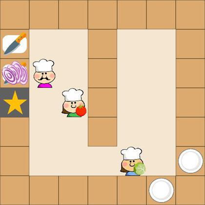
(f) (f) The pink agent finishes chopping the onion, and then it executes Get-Onion to pick it up.

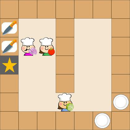
(g) (g) After picking up the onion, the pink agent executes Get-Plate-1.

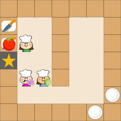
(h) (h) After putting the tomato on the cutting board, the green agent executes Chop.

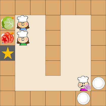
(i) (i) After putting the lettuce on the cutting board, the blue agent executes Chop.

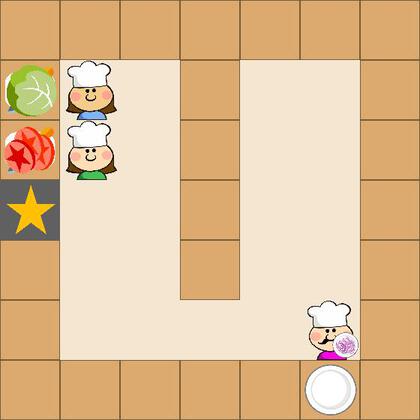
(j) (j) The pink agent puts the onion on the plate, and then executes Go-Cut-Board-2. The blue agent executes Go-Cut-Board-2. The green agent executes Go-Cut-Board-1.

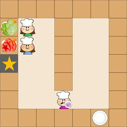
(k) (k) The green agent executes Get-Lettuce.

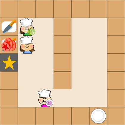
(l) (l) After picking up the lettuce, the green agent executes Go-Counter.

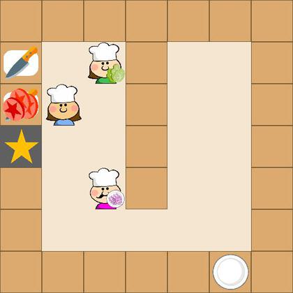
(a) (m) The blue agent executes Go-Cut-Board-1 to make room for the pink agent.

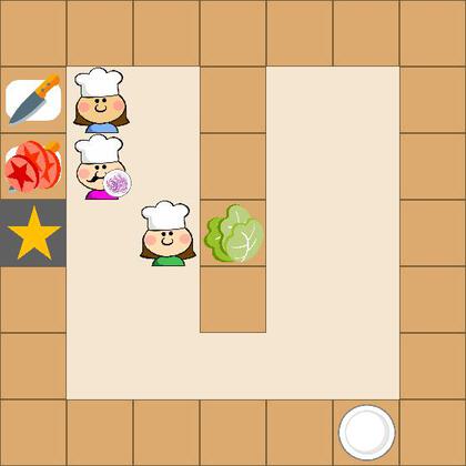
(b) (n) The green agent puts the lettuce on the counter

(c) (o) After merging the tomato into the plate, the pink agent executes Get-Lettuce. Meanwhile the green agent steps away to make room for the pink agent.

(d) (p) After getting the lettuce, the pink agent executes Deliver.

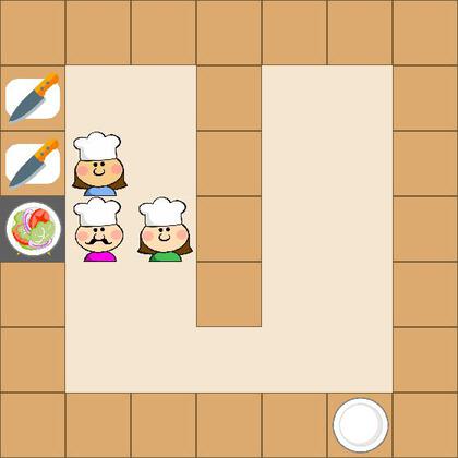
(e) (q) The pink agent successfully delivers the tomato-lettuce-onion salad.

Figure 31: Visualization of running decentralized policies learned by Mac-IAICC in Overcooked-C.

G.3 Warehouse Tool Delivery

Warehouse A:

(a) (a) Initial State.

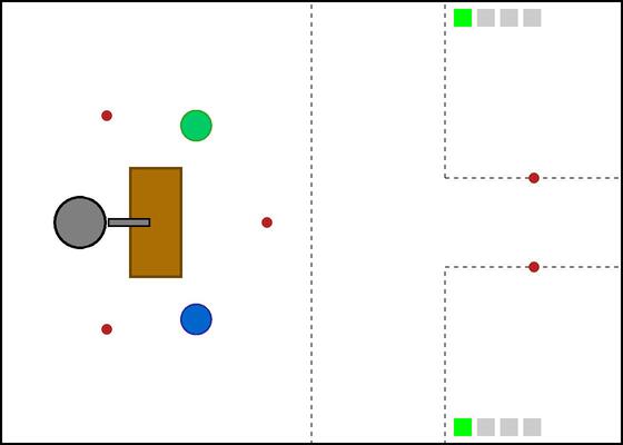
(b) (b) Mobile robots moves towards the table by running Get-Tool, and arm robot runs Search-Tool(0) to find Tool-0.

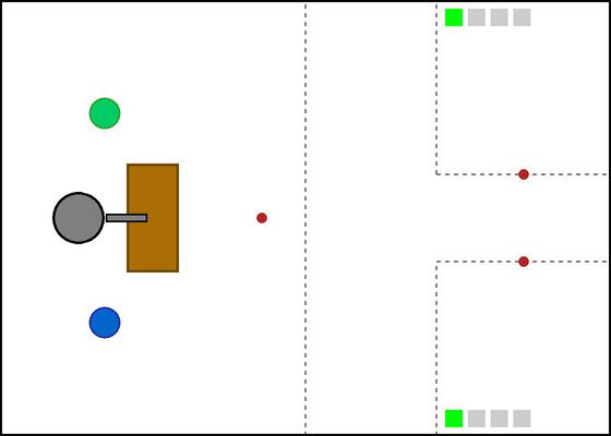
(c) (c) Mobile robots wait there and arm robot keeps looking for Tool-0.

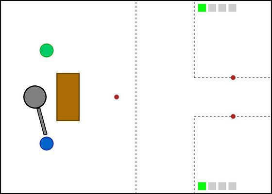
(d) (d) Arm robot executes Pass-to-M(1) to pass Tool-0 to the blue robot.

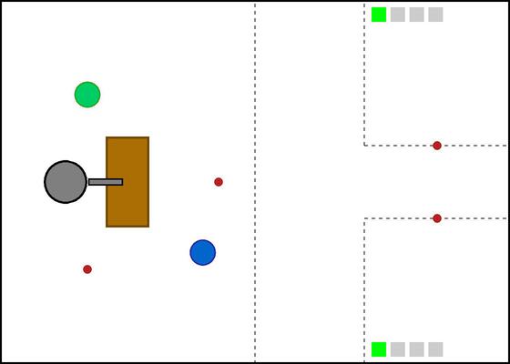
(e) (e) Arm robot executes Search-Tool(0) to find Tool-0, and blue robot moves to workshop-1 by executing Go-W(1).

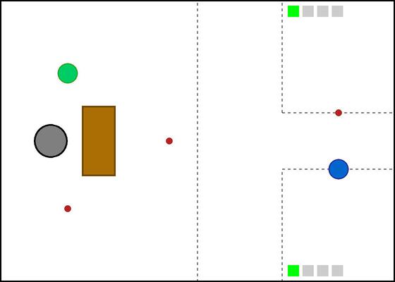
(f) (f) Blue robot successfully delivers Tool-0 to workshop-1.

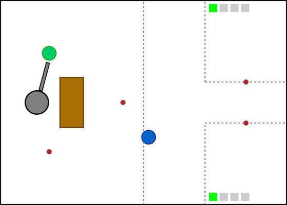
(g) (g) Blue robot runs Get-Tool to go back table, and arm robot executes Pass-to-M(0) to pass Tool-0 to green robot.

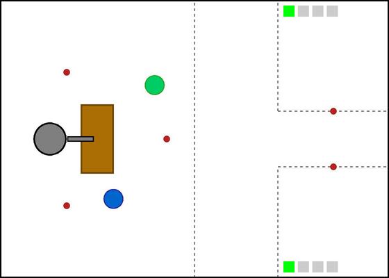
(h) (h) Green robot executes Go-W(0) and arm robot runs Search-Tool(1).

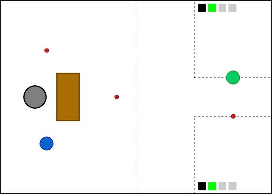
(i) (i) Green robot successfully delivers Tool-0 to workshop-0. Human-0 and human-1 finish subtask-0 and start to do subtask-1 with delivered Tool-0.

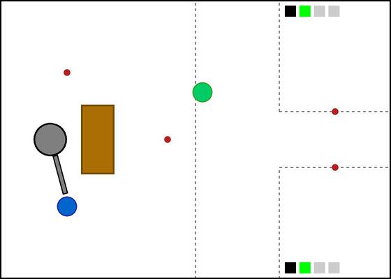
(j) (j) Green robot runs Get-Tool to go back table, and arm robot executes Pass-to-M(1) to pass a Tool-1 to blue robot.

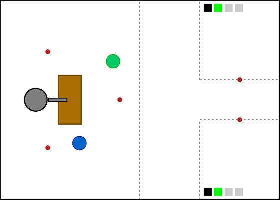
(k) (k) Blue robot executes Go-W(1) and arm robot runs Search-Tool(1).

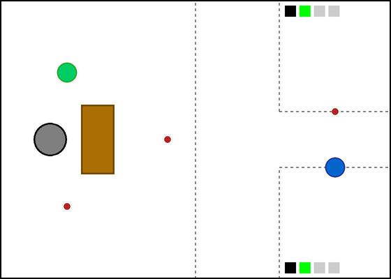
(l) (l) Blue robot successfully delivers a Tool-1 to workshop-1.

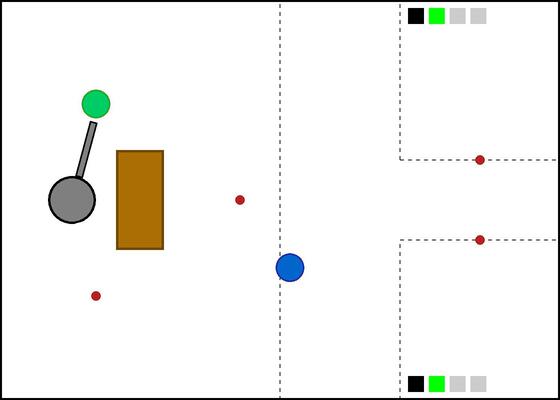
(a) (m) Arm robot executes Pass-to-M(0) to pass Tool-1 to green robot. Blue robot runs Get-Tool to go back table.

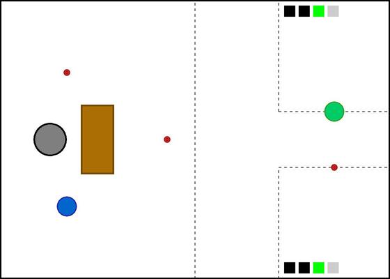
(b) (n) Green robot successfully delivers Tool-1 to workshop-0. Human-0 and human-1 finish subtask-1 and start to do subtask-2 with delivered Tool-1.

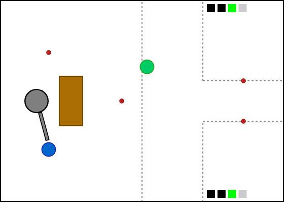
(c) (o) Arm robot executes Pass-to-M(1) to pass Tool-2 to blue robot. Green robot runs Get-Tool to go back table.

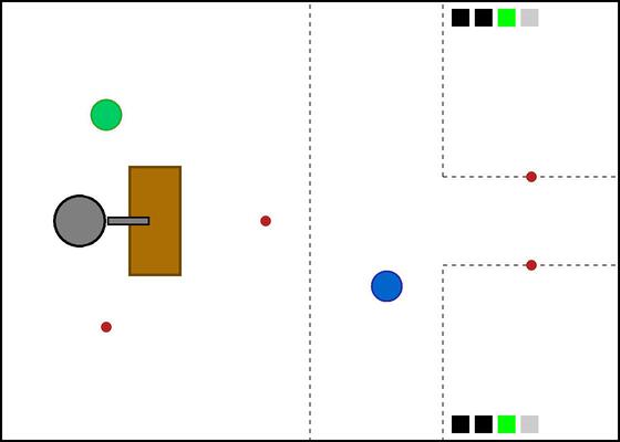
(d) (p) Blue robot executes Go-W(1). Arm robot runs Search-Tool(2).

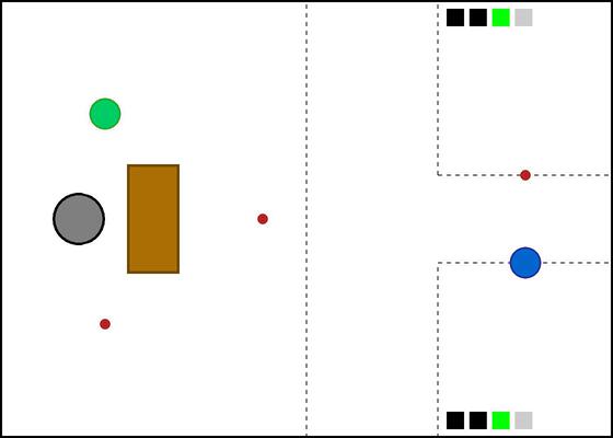
(e) (q) Blue robot successfully delivers Tool-2 to human-0.

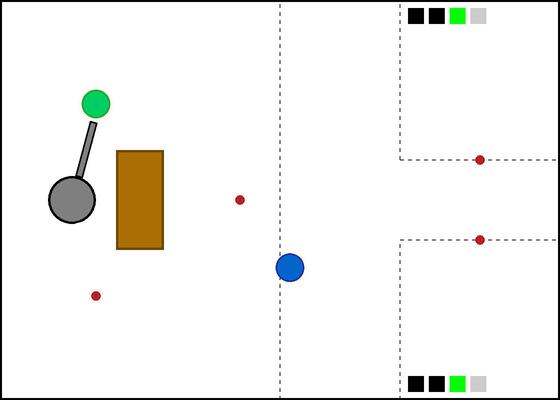
(f) (r) Arm robot executes Pass-to-M(0) to pass Tool-2 to green robot. Blue robot runs Get-Tool to go back table.

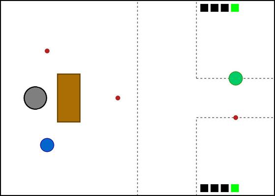
(g) (s) Green robot directly goes to workshop-0 by running Go-W(0) and finishes the last tool delivery for human-0. The entire task is done.

Warehouse-B:.

(a) (a) Initial State.

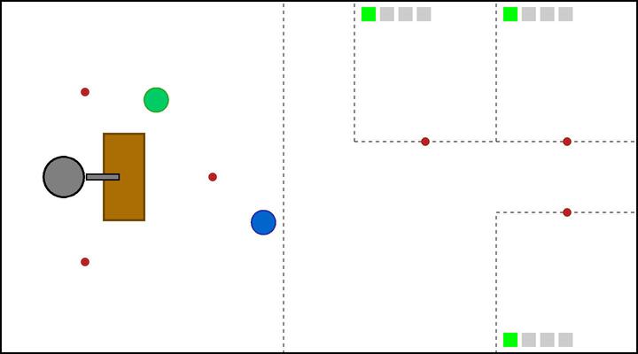
(b) (b) Green robot moves towards the table by running Get-Tool. Blue robot moves to workshop-0 by executing Go-W(0). Arm robot runs Search-Tool(0) to find Tool-0.

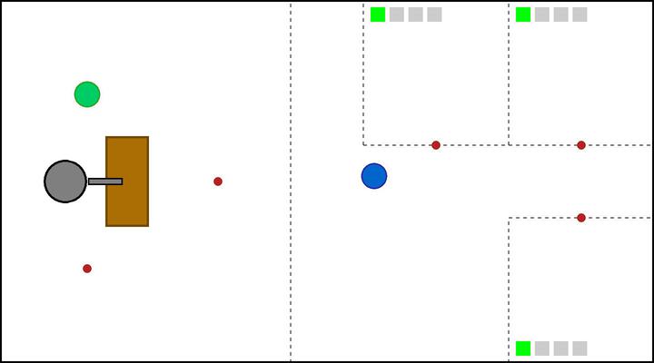
(c) (c) Green robot waits there and arm robot keeps looking for Tool-0.

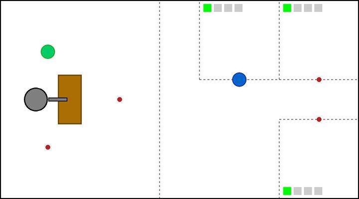
(d) (d) Blue robot reaches workshop-0.

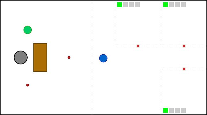
(e) (e) Blue robot runs Get-Tool to go back table.

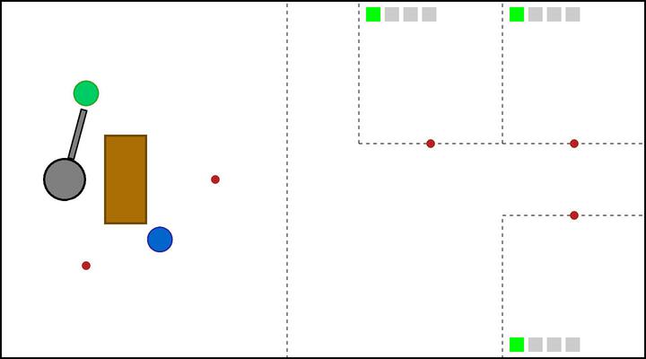
(f) (f) Arm robot executes Pass-to-M(0) to pass Tool-0 to green robot.

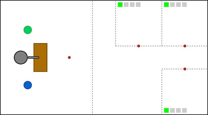
(g) (g) Arm robot runs Search-Tool(0) to find the 2nd Tool-0.

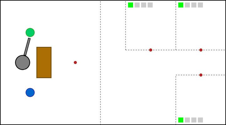
(h) (h) Arm robot executes Pass-to-M(0) to pass the 2nd Tool-0 to green robot.

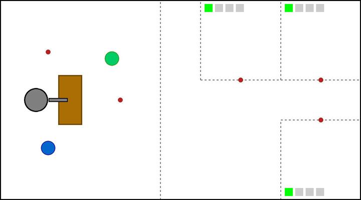
(i) (i) Arm robot runs Search-Tool(0) to find the the 3rd Tool-0. Green robot moves to workshop-1 by executing Go-W(1).

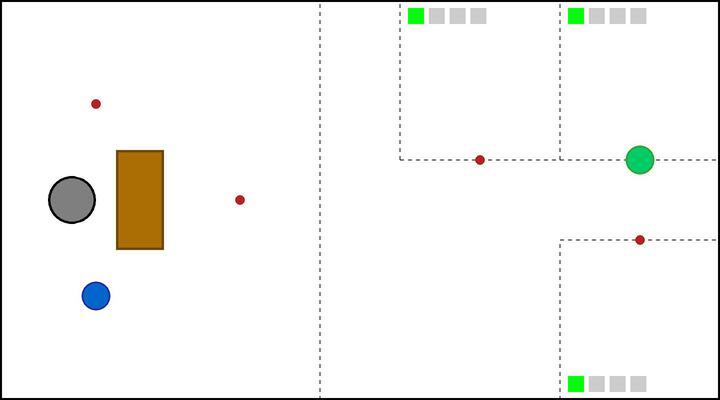
(j) (j) Green robot successfully delivers Tool-0 to workshop-1.

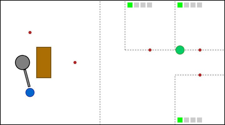
(k) (k) Arm robot executes Pass-to-M(1) to pass the 3rd Tool-0 to blue robot. Green robot moves to workshop-0 by executing Go-W(0).

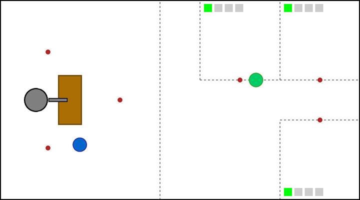
(l) (l) Arm robot runs Search-Tool(1) to find Tool-1. Blue robot moves to workshop-2 by executing Go-W(2).

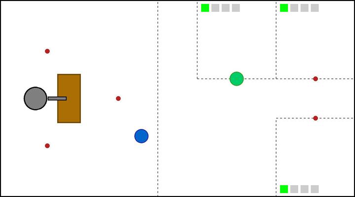
(a) (m) Green robot successfully delivers a Tool-0 to workshop-0.

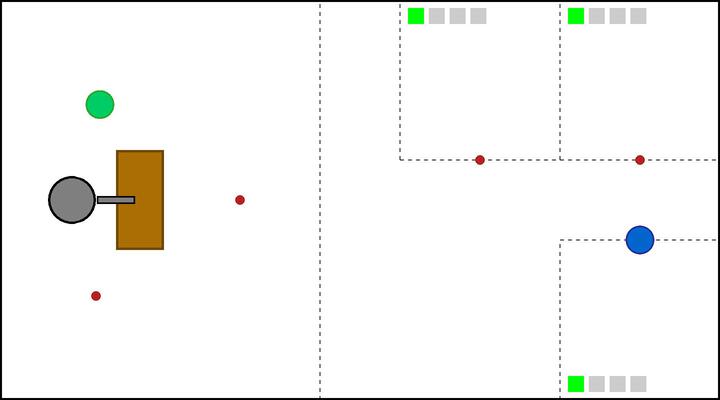
(b) (n) Blue robot successfully delivers a Tool-0 to workshop-2. Arm robot runs Search-Tool(1) to find another Tool-1.

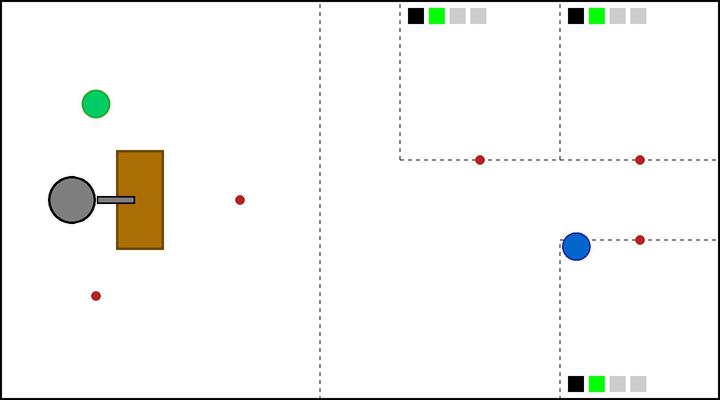
(c) (o) Blue robot runs Get-Tool to go back table. All humans finish subtask-0 and start to do subtask-1.

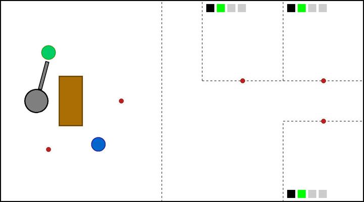
(d) (p)Arm robot executes Pass-to-M(0) to pass a Tool-1 to green robot.

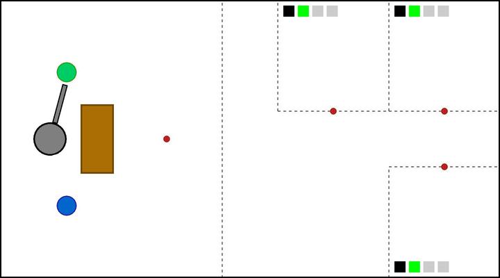
(e) (q) Arm robot executes Pass-to-M(0) to pass another Tool-1 to green robot.

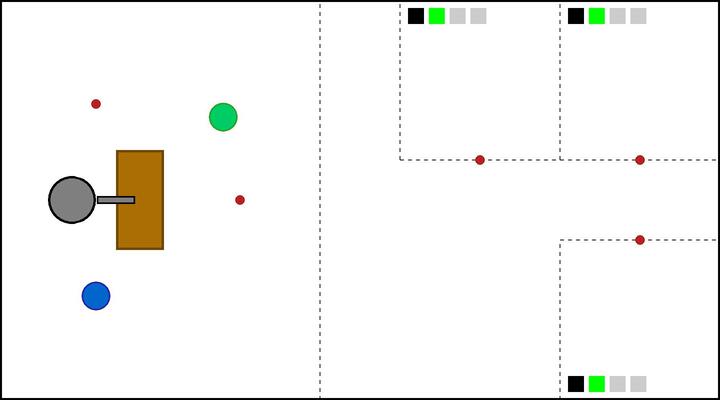
(f) (r) Green robot moves to workshop-1 by executing Go-W(1). Arm robot runs Search-Tool(1) to find the 3rd Tool-1.

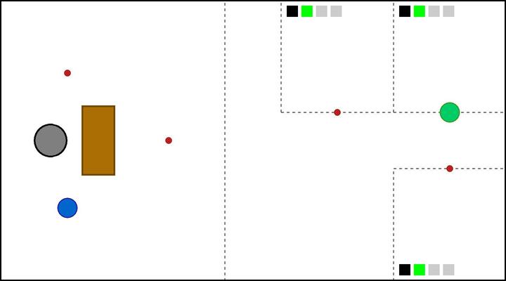
(g) (s) Green robot successfully delivers a Tool-0 to workshop-0.

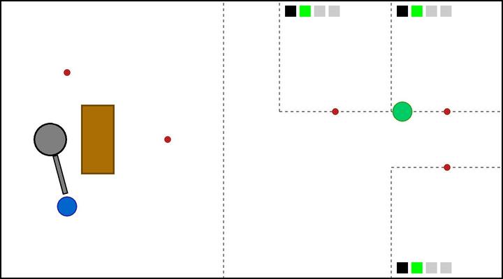
(h) (t) Green robot moves to workshop-0 by executing Go-W(0). Arm robot executes Pass-to-M(1) to pass the 3rd Tool-1 to blue robot.

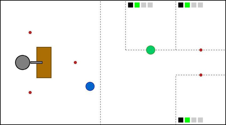
(i) (u) Arm robot runs Search-Tool(2) to find Tool-2. Green robot successfully delivers a Tool-1 to workshop-0. Blue robot moves to workshop-2 by executing Go-W(2).

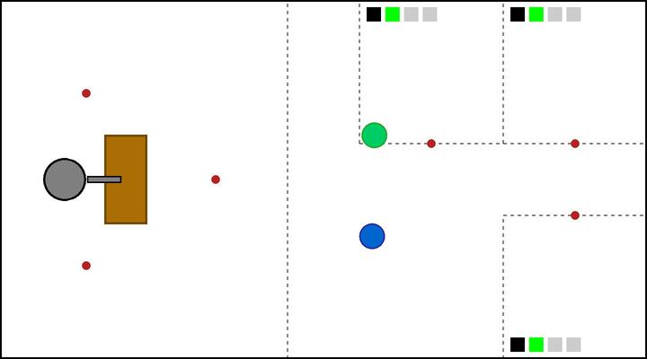
(j) (v) Green robot runs Get-Tool to go back table.

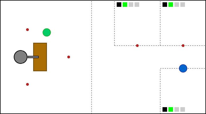
(k) (w) Arm robot runs Search-Tool(2) to find another Tool-2. Blue robot successfully delivers a Tool-1 to workshop-2.

(l) (x) Blue robot runs Get-Tool to go back table.

(m) (y) Arm robot executes Pass-to-M(0) to pass a Tool-2 to green robot.

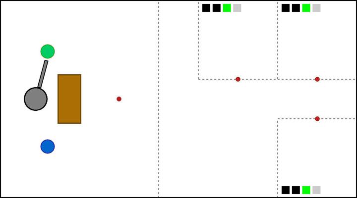
(n) (z) Arm robot executes Pass-to-M(0) to pass another Tool-2 to green robot. All humans finish subtask-1 and start to do subtask-2.

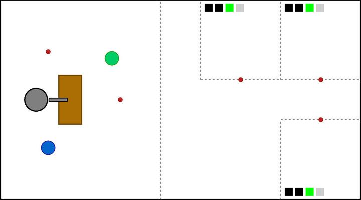
(o) (A) Arm robot runs Search-Tool(2) to find the 3rd Tool-2. Green robot moves to workshop-1 by executing Go-W(1).

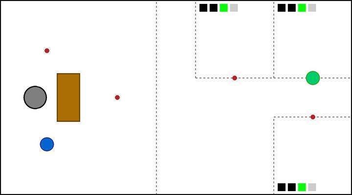
(a) (B) Green robot successfully delivers a Tool-2 to workshop-1.

(b) (C) Arm robot executes Pass-to-M(1) to pass the 3rd Tool-2 to blue robot.

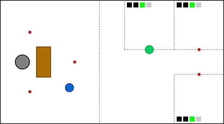
(c) (D) Green robot successfully delivers a Tool-2 to workshop-0. Blue robot moves to workshop-2 by executing Go-W(2).

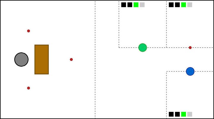
(d) (E) Blue robot successfully delivers a Tool-2 to workshop-2. Humans have received all tools, and for robots, the task is done.

Warehouse-C:

(a) (a) Initial State.

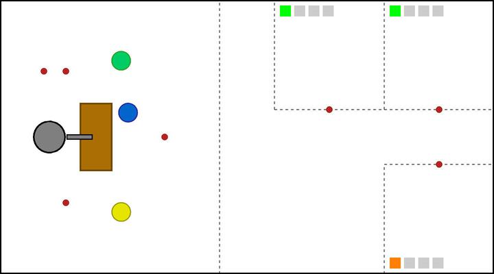
(b) (b) Mobile robots move towards the table by running Get-Tool. Arm robot runs Search-Tool(0) to find the 1st Tool-0.

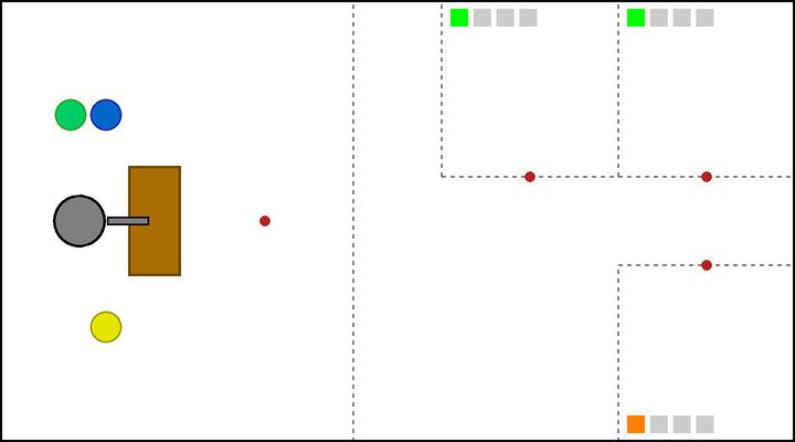
(c) (c) Mobile robots wait there and arm robot keeps looking for the 1st Tool-0.

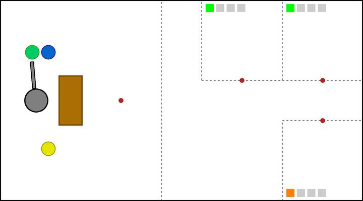
(d) (d) Arm robot executes Pass-to-M(0) to pass a Tool-0 to green robot.

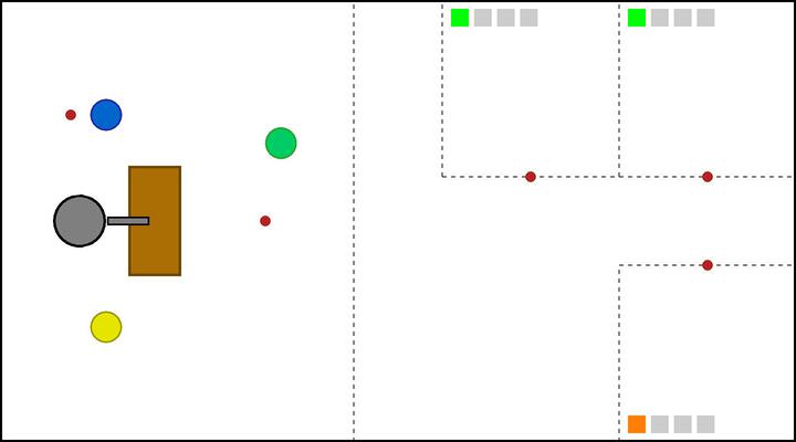
(e) (e) Arm robot runs Search-Tool(0) to find the 2nd Tool-0. Green robot moves to workshop-0 by executing Go-W(0).

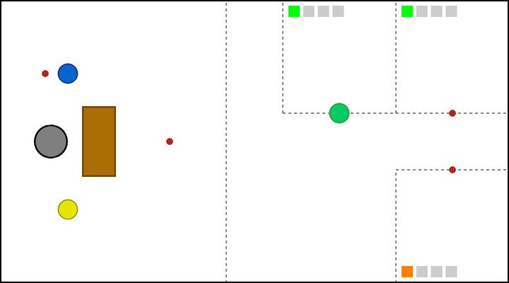
(f) (f) Green robot successfully delivers the a Tool-0 to workshop-0.

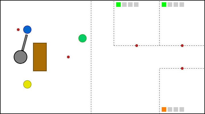
(g) (g) Green robot runs Get-Tool to go back table. Arm robot executes Pass-to-M(1) to pass a Tool-0 to blue robot.

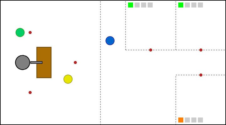
(h) (h) Arm robot runs Search-Tool(0) to find the 3rd Tool-0. Blue robot moves to workshop-1 by executing Go-W(1). Yellow robot moves to workshop-0 by executing Go-W(0).

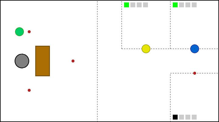
(i) (i) Blue robot successfully delivers the a Tool-0 to workshop-1. Yellow robot reaches workshop-0 and observes that human-0 has got Tool-0. Human-2 finishes subtask-0 and waits for Tool-0.

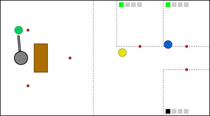
(j) (j) Arm robot executes Pass-to-M(0) to pass a Tool-0 to green robot. Yellow and blue robots run Get-Tool to go back table.

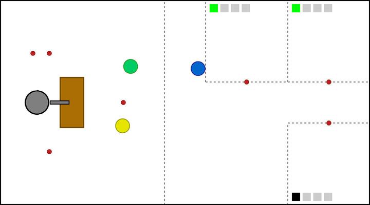
(k) (k) Arm robot runs Search-Tool(1) to find the 1st Tool-1. Green robot moves to workshop-0 by executing Go-W(0).

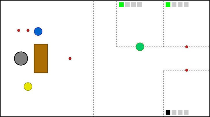
(l) (l) Green robot reaches workshop-0 and observes that human-0 does not need Tool-0.

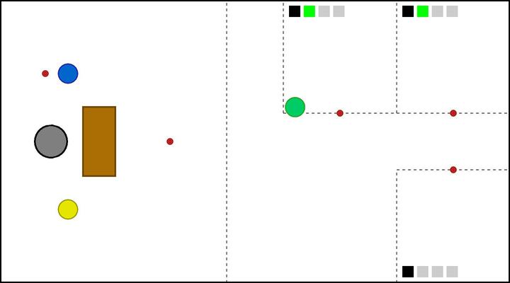
(a) (m) Green robot runs Get-Tool to go back table.

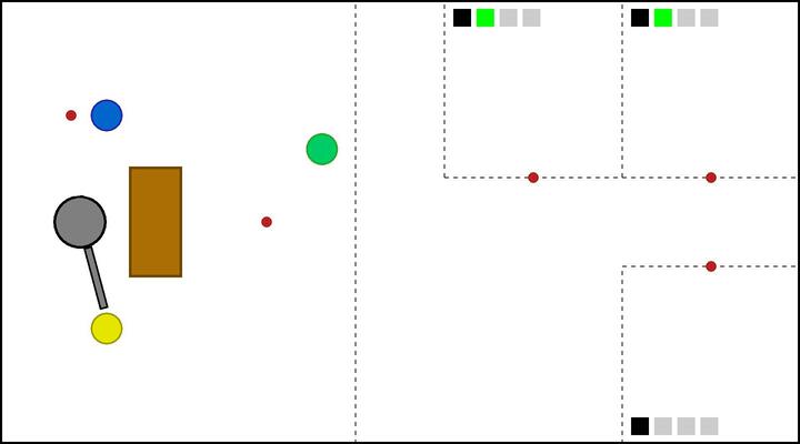
(b) (n) Arm robot executes Pass-to-M(2) to pass a Tool-1 to yellow robot.

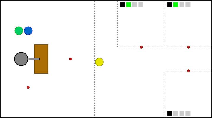
(c) (o) Arm robot runs Search-Tool(1) to find the 2nd Tool-1. Yellow robot moves to workshop-0 by executing Go-W(0).

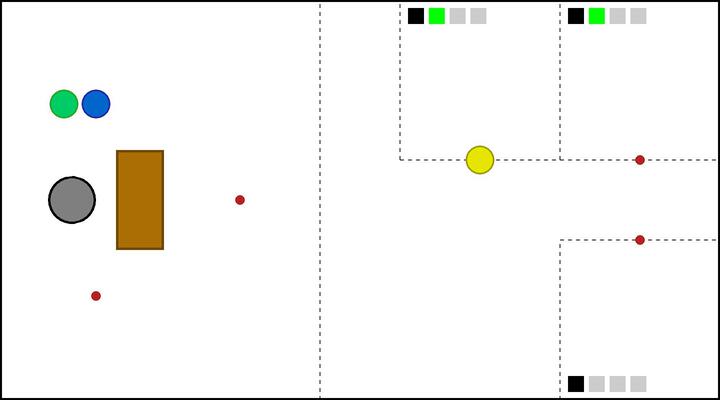
(d) (p) Yellow robot successfully delivers the a Tool-1 to workshop-0.

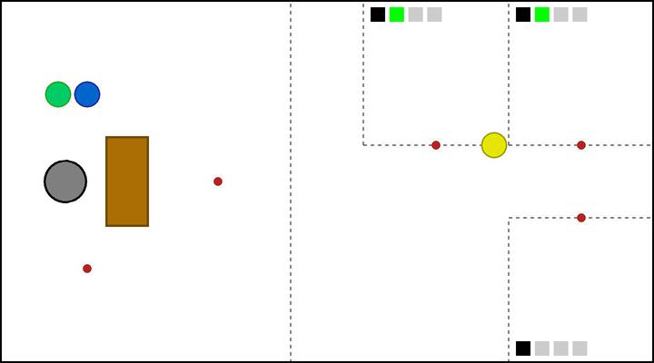
(e) (q) Yellow robot moves to workshop-1 by executing Go-W(1).

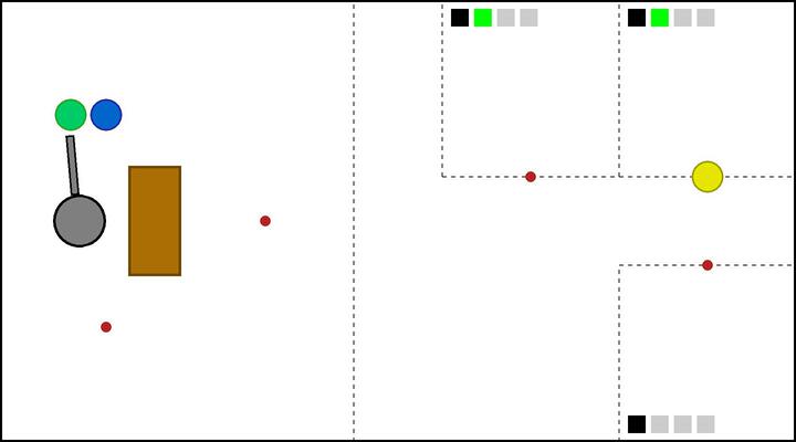
(f) (r) Arm robot executes Pass-to-M(0) to pass a Tool-1 to green robot.

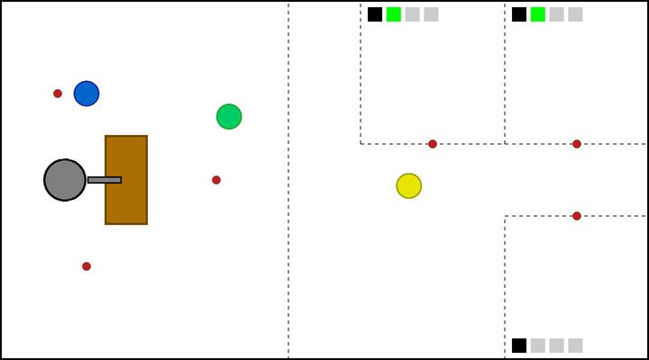
(g) (s) Arm robot runs Search-Tool(1) to find 3st Tool-1. Yellow robot runs Get-Tool to go back table. Green robot moves to workshop-0 by executing Go-W(0).

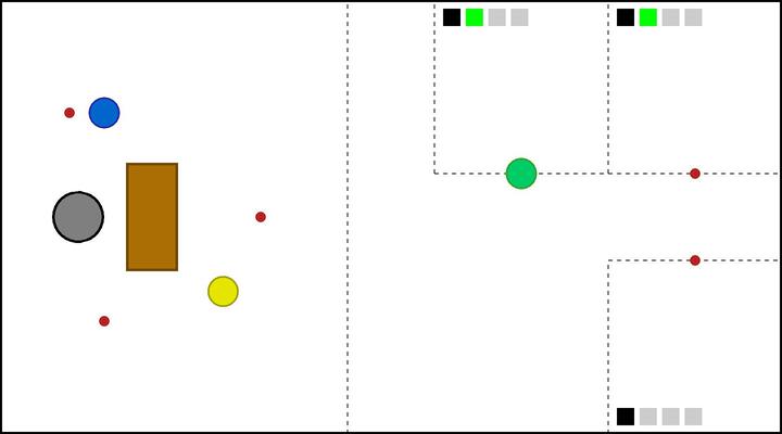
(h) (t) Green robot successfully delivers a Tool-1 to workshop-0.

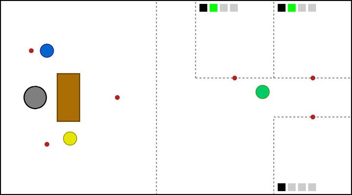
(i) (u) Green robot moves to workshop-2 by executing Go-W(2).

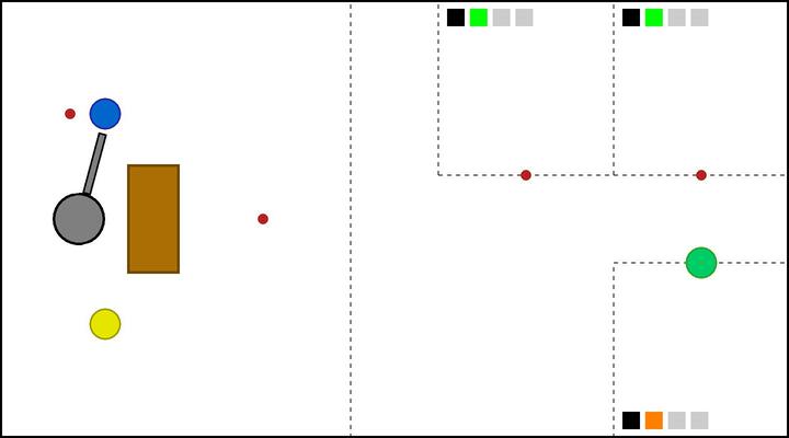
(j) (v) Green robot successfully delivers the a Tool-0 to workshop-2. Human-2 finishes subtask-0 and starts to do subtask-1. Arm robot executes Pass-to-M(1) to pass a Tool-1 to blue robot.

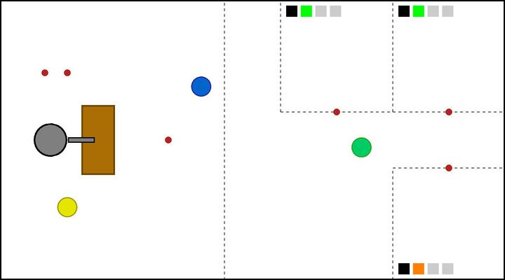
(k) (w) Green robot runs Get-Tool to go back table. Arm robot runs Search-Tool(2) to find the 1st Tool-2. Blue robot moves to workshop-1 by executing Go-W(1).

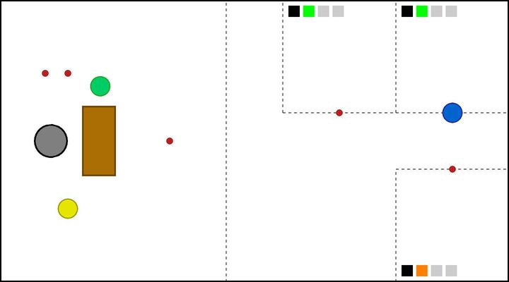
(l) (x) Blue robot successfully delivers a Tool-1 to workshop-1.

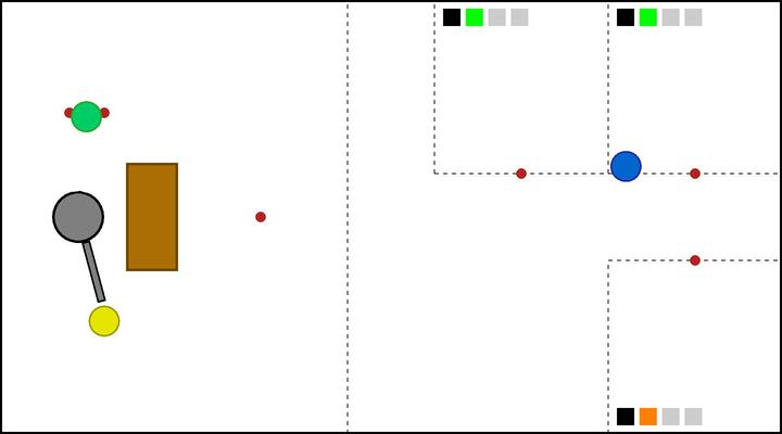
(m) (y) Blue robot runs Get-Tool to go back table. Arm robot executes Pass-to-M(2) to pass a Tool-2 to yellow robot.

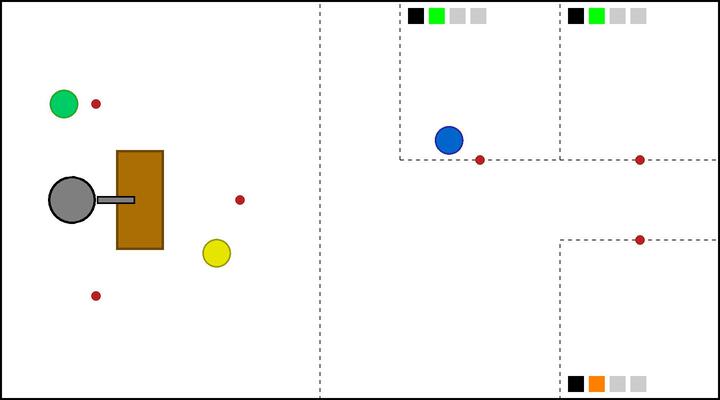
(n) (z) Arm robot runs Search-Tool(2) to find the 2nd Tool-2. Yellow robot moves to workshop-1 by executing Go-W(1).

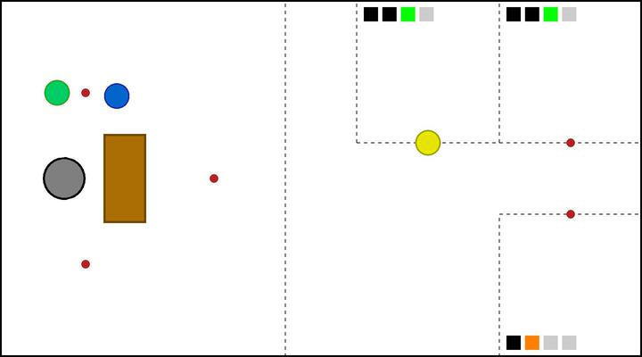
(o) (A) Yellow robot successfully delivers a Tool-2 to workshop-0. Human-0 and human-1 finish subtask-1 and start to do subtask-2.

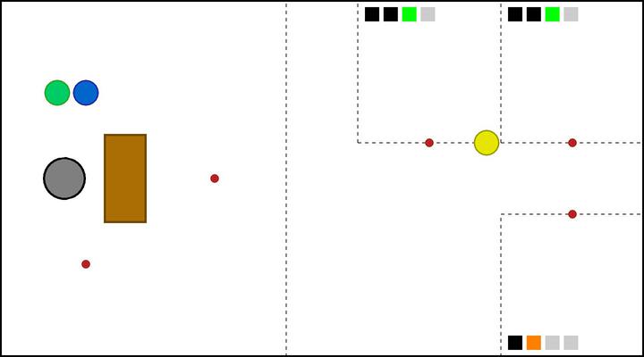
(a) (B) Yellow robot moves to workshop-1 by executing Go-W(1).

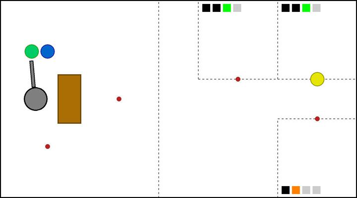
(b) (C) Arm robot executes Pass-to-M(0) to pass a Tool-2 to green robot. Yellow robot reaches workshop-1 but it does not have any tool.

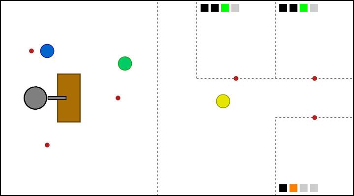
(c) (D) Arm robot runs Search-Tool(2) to find the 3rd Tool-2. Green robot moves to workshop-0 by executing Go-W(0). Yellow robot runs Get-Tool to go back table.

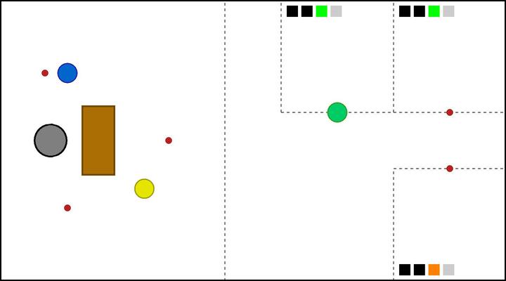
(d) (E) Green robot reaches workshop-0 and observes that human-0 does not need Tool-2. Human-2 finishes subtask-1 and starts to do subtask-2.

(e) (F) Green robot moves to workshop-2 by executing Go-W(2).

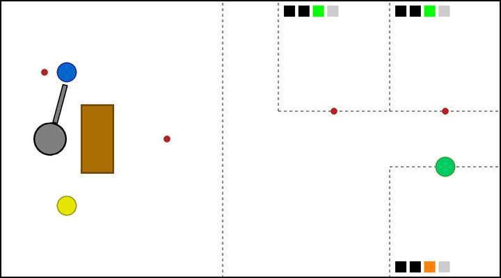
(f) (G) Green robot successfully delivers a Tool-2 to workshop-2. Arm robot executes Pass-to-M(1) to pass a Tool-2 to blue robot.

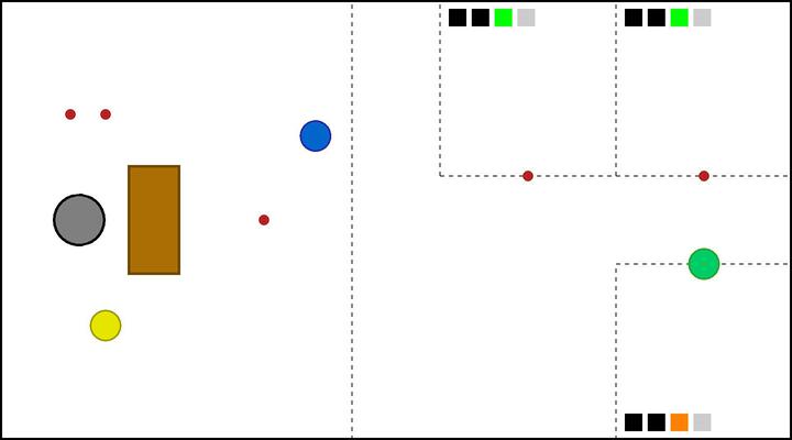
(g) (H) Blue robot moves to workshop-1 by executing Go-W(1).

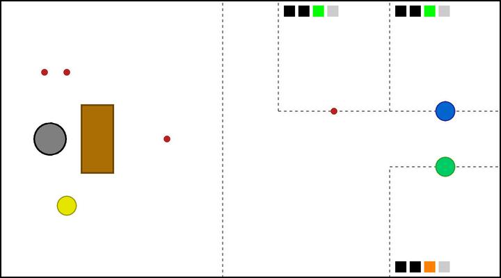
(h) (I) Blue robot successfully delivers a Tool-2 to workshop-1. Humans have received all tools, and for robots, the task is done.

Warehouse-D:

(a) (a) Initial State.

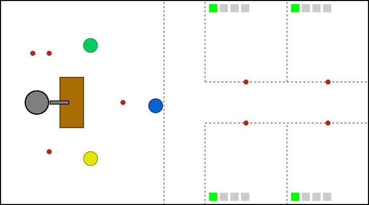
(b) (b) Green and yellow robots move towards the table by running Get-Tool. Blue robot moves to workshop-3 by executing Go-W(3). Arm robot runs Search-Tool(0) to find the 1st Tool-0.

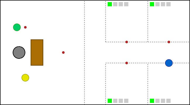
(c) (c) Blue robot reaches workshop-3.

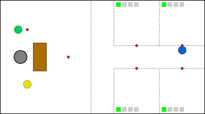
(d) (d) Blue robot moves to workshop-1 by executing Go-W(1).

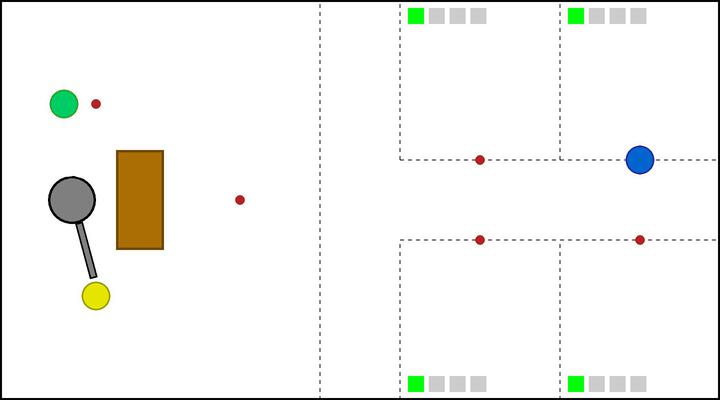
(e) (e) Blue robot reaches workshop-1. Arm robot executes Pass-to-M(2) to pass a Tool-0 to yellow robot.

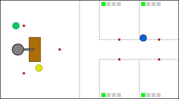
(f) (f) Arm robot runs Search-Tool(0) to find the 2nd Tool-0. Blue robot runs Get-Tool to go back table. Yellow robot moves to workshop-1 by executing Go-W(1).

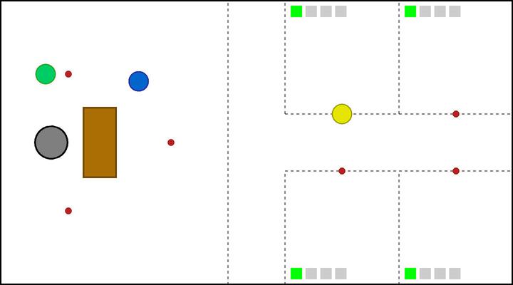
(g) (g) Yellow robot successfully delivers a Tool-0 to workshop-0.

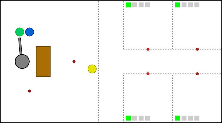
(h) (h) Arm robot executes Pass-to-M(0) to pass a Tool-0 to green robot. Yellow robot runs Get-Tool to go back table.

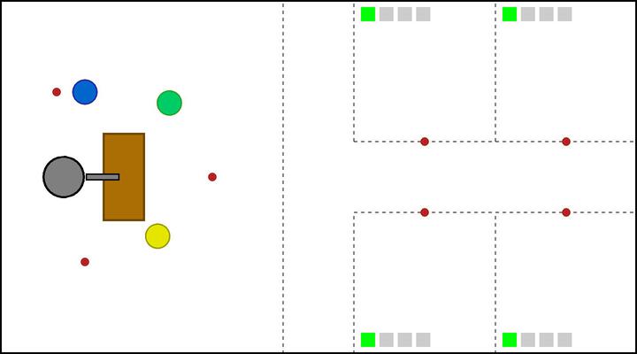
(i) (i) Arm robot runs Search-Tool(0) to find the 3rd Tool-0. Green robot moves to workshop-1 by executing Go-W(1).

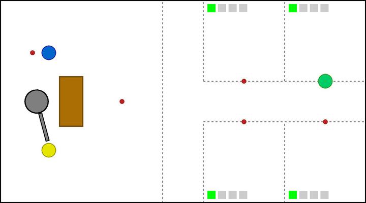
(j) (j) Green robot successfully delivers the a Tool-0 to workshop-1. Arm robot executes Pass-to-M(2) to pass a Tool-0 to yellow robot.

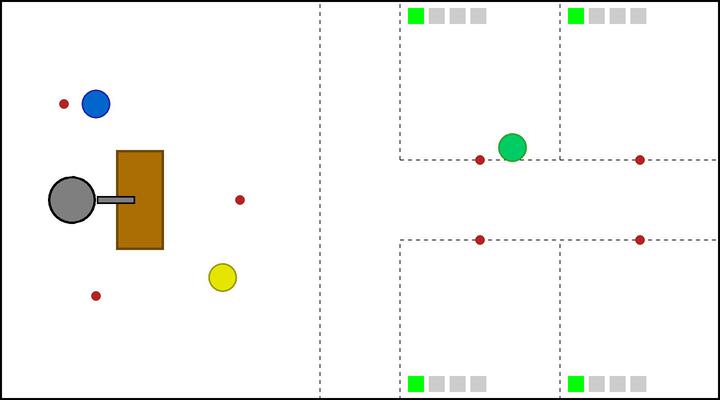
(k) (k) Arm robot runs Search-Tool(1) to find the 1st Tool-1. Yellow robot moves to workshop-2 by executing Go-W(2). Green robot runs Get-Tool to go back table.

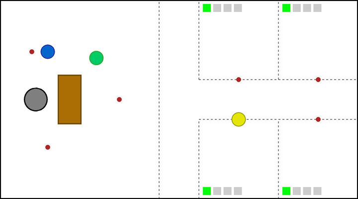
(l) (l) Yellow robot successfully delivers a Tool-0 to workshop-2.

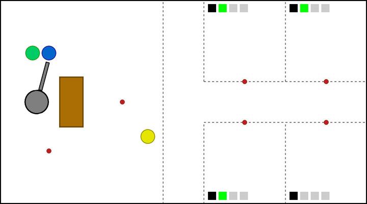
(a) (m) Yellow robot runs Get-Tool to go back table. Arm robot executes Pass-to-M(1) to pass the a Tool-1 to blue robot. Human-0, human-1 and human-2 finish subtask-0 and start to do subtask-1.

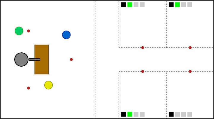
(b) (n) Arm robot runs Search-Tool(1) to find the 2nd Tool-1. Blue robot moves to workshop-1 by executing Go-W(1).

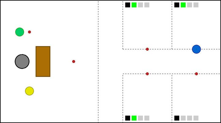
(c) (o) Blue robot successfully delivers a Tool-1 to workshop-1.

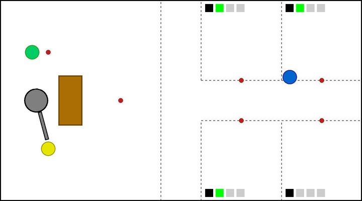
(d) (p)Arm robot executes Pass-to-M(2) to pass a Tool-1 to yellow robot. Blue robot runs Get-Tool to go back table.

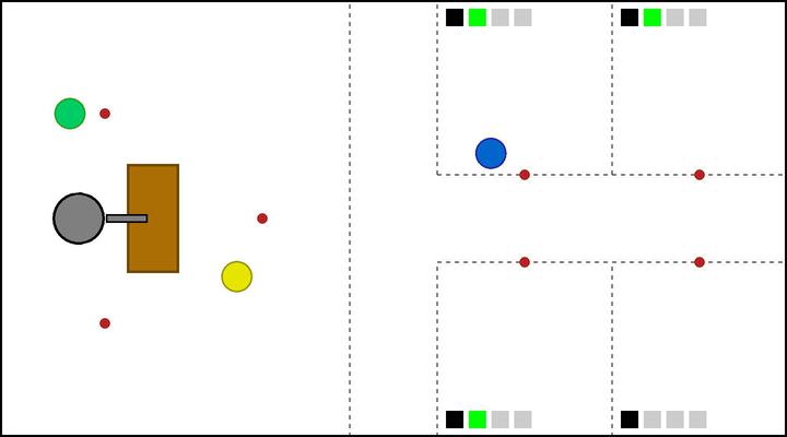
(e) (q) Arm robot runs Search-Tool(0) to find 4th Tool-0. Yellow robot moves to workshop-0 by executing Go-W(0).

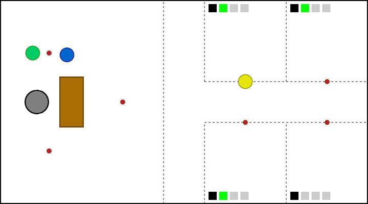
(f) (r) Yellow robot successfully delivers a Tool-1 to workshop-0.

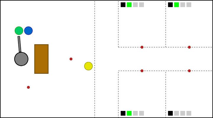
(g) (s) Yellow robot runs Get-Tool to go back table. Arm robot executes Pass-to-M(0) to pass a Tool-0 to green robot.

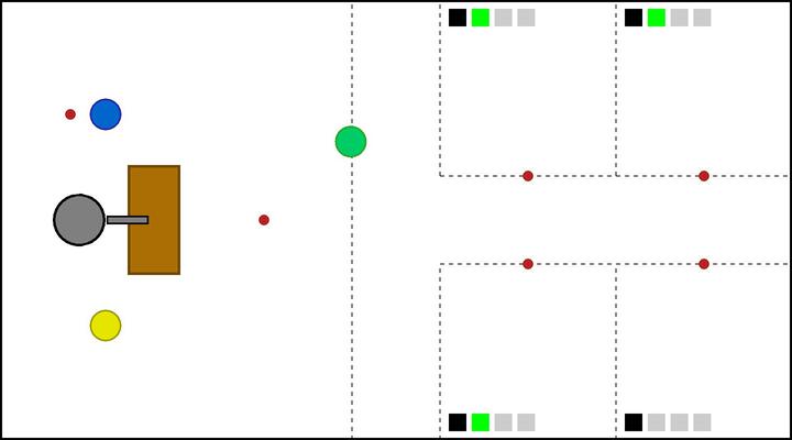
(h) (t) Arm robot runs Search-Tool(1) to find the 3rd Tool-1. Green robot moves to workshop-1 by executing Go-W(1).

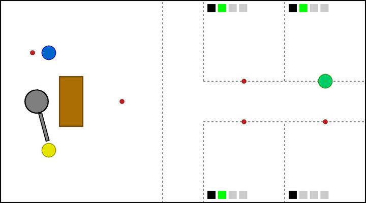
(i) (u) Green robot reaches workshop-1 and observes that human-1 does not need Tool-0 and it moves to workshop-3 by executing Go-W(3). Arm robot executes Pass-to-M(2) to pass a Tool-1 to yellow robot.

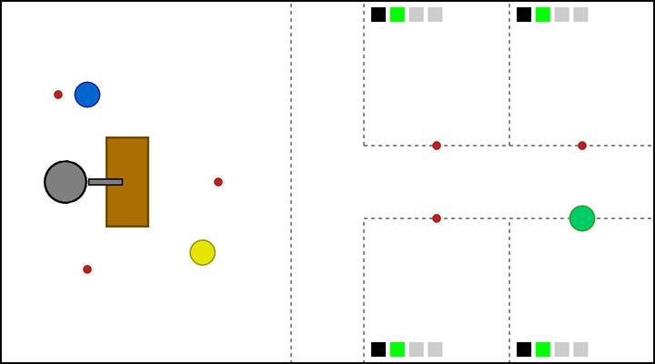
(j) (v) Arm robot runs Search-Tool(1) to find the 4th Tool-1. Green robot successfully delivers a Tool-0 to workshop-3. Human-3 finishes subtask-0 and starts to do subtask-1. Yellow robot moves to workshop-2 by executing Go-W(2).

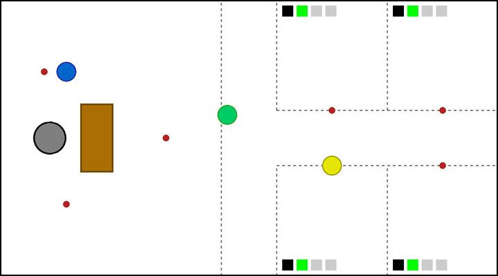
(k) (w) Yellow robot successfully delivers a Tool-1 to workshop-2. Green robot runs Get-Tool to go back table.

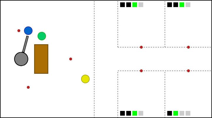
(l) (x) Arm robot executes Pass-to-M(1) to pass a Tool-1 to blue robot. Yellow robot runs Get-Tool to go back table.

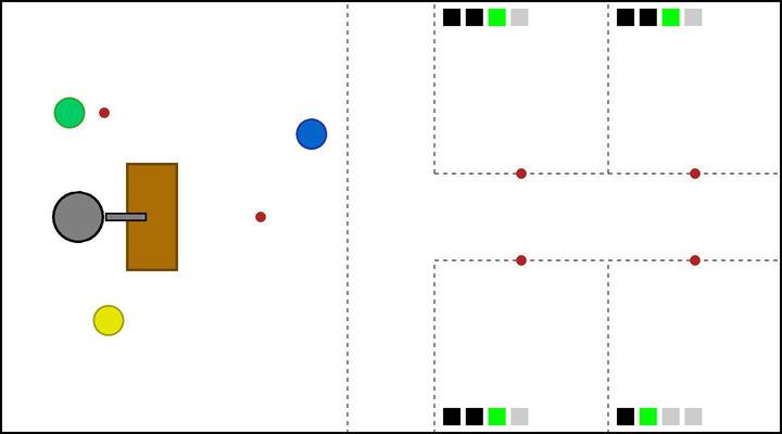
(a) (y) Arm robot runs Search-Tool(2) to find the 1st Tool-2. Blue robot moves to workshop-1 by executing Go-W(1).

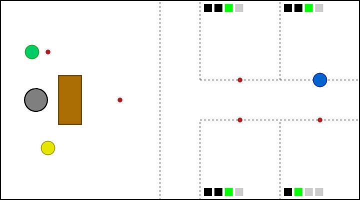
(b) (z) Blue robot reaches workshop-1 and observes that human-1 does not need Tool-1.

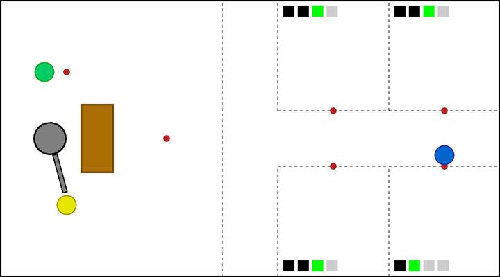
(c) (A) Arm robot executes Pass-to-M(2) to pass a Tool-2 to yellow robot. Blue robot moves to workshop-3 by executing Go-W(3).

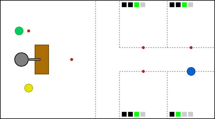
(d) (B) Arm robot runs Search-Tool(2) to find the 2nd Tool-2. Blue robot successfully delivers a Tool-1 to workshop-3.

(e) (C) Blue robot moves to workshop-1 by executing Go-W(1).

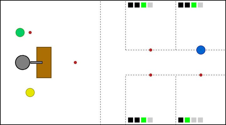
(f) (D) Blue robot reaches workshop-1.

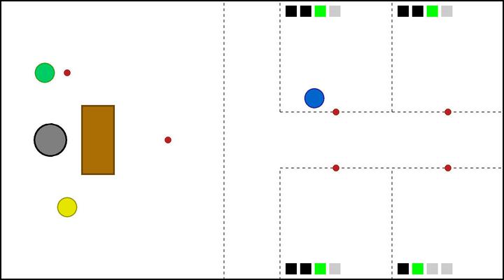
(g) (E) Blue robot runs Get-Tool to go back table.

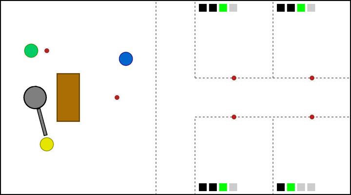
(h) (F) Arm robot executes Pass-to-M(2) to pass the a Tool-2 to yellow robot.

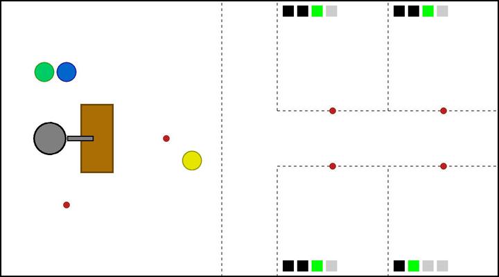
(i) (G) Arm robot runs Search-Tool(2) to find the 3rd Tool-2. Yellow robot moves to workshop-1 by executing Go-W(1).

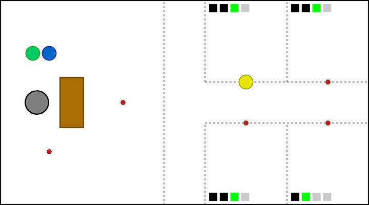
(j) (H) Yellow robot reaches workshop-0 and observes that human-0 has got a Tool-2.

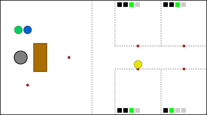
(k) (I) Yellow robot moves to workshop-2 by executing Go-W(2).

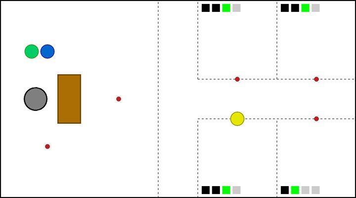
(l) (J) Yellow robot successfully delivers a Tool-2 to workshop-2.

(m) (K) Arm robot executes Pass-to-M(0) to pass a Tool-2 to green robot. Yellow robot runs Get-Tool to go back table.

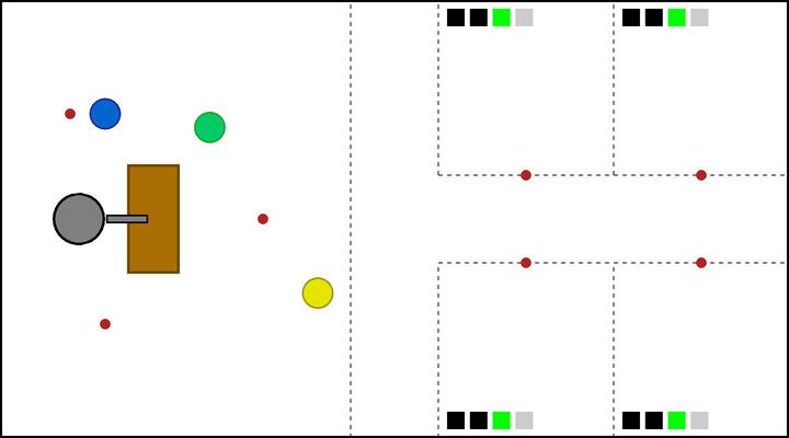
(n) (L) Arm robot runs Search-Tool(2) to find the 4th Tool-2. Green robot moves to workshop-1 by executing Go-W(1).

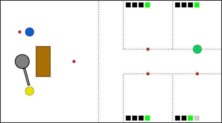
(o) (M) Arm robot executes Pass-to-M(2) to pass a Tool-2 to yellow robot. Green robot successfully delivers a Tool-2 to workshop-1. Human-0, human-1 and human-2 finish subtask-2 and starts to do subtask-3.

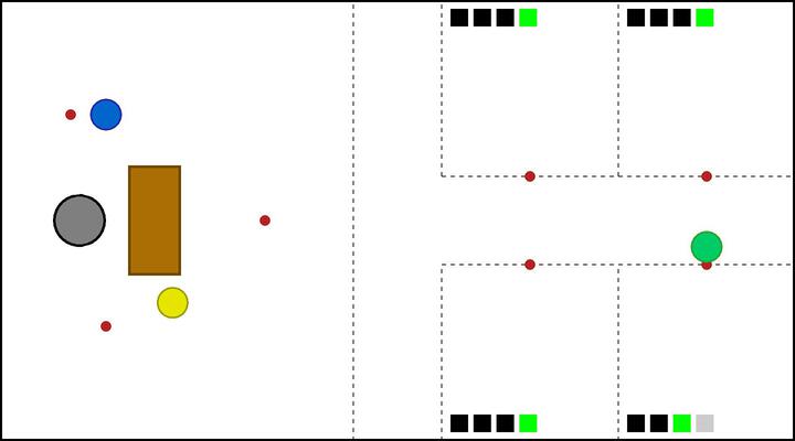
(a) (N) Yellow robot moves to workshop-0 by executing Go-W(0). Green robot moves to workshop-3 by executing Go-W(3).

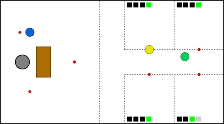
(b) (O) Yellow robot reaches workshop-0 and observes that human-0 does not need Tool-2.

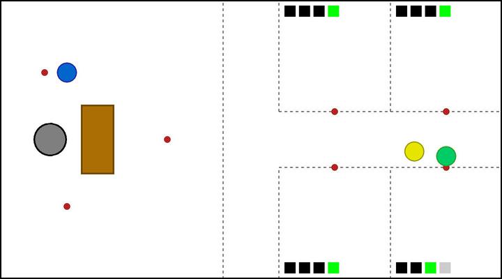
(c) (P) Yellow and green robot move to workshop-3 by executing Go-W(3).

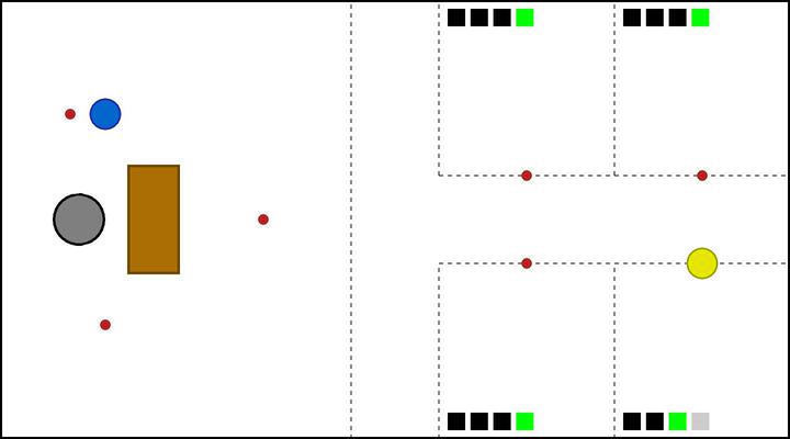
(d) (Q) Yellow robot successfully delivers a Tool-2 to workshop-3. Humans have received all tools, and for robots, the task is done.

Warehouse-E:

(a) (a) Initial State.

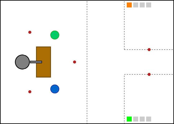
(b) (b) Mobile robots moves towards the table by running Get-Tool, and arm robot runs Search-Tool(0) to find Tool-0.

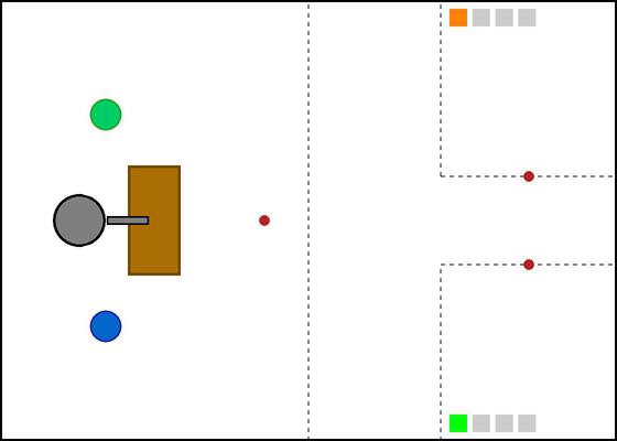
(c) (c) Mobile robots wait there and arm robot keeps looking for Tool-0.

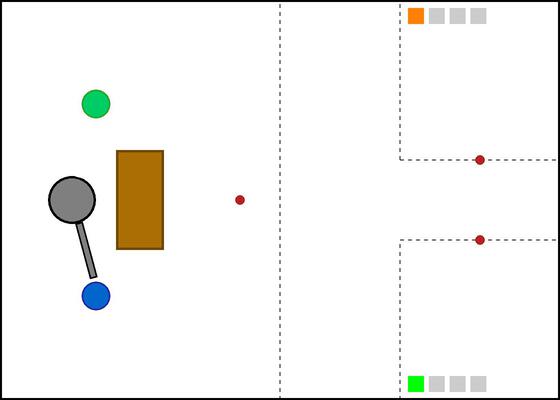
(d) (d) Arm robot executes Pass-to-M(1) to pass Tool-0 to the blue robot.

(e) (e) Arm robot runs Search-Tool(1) to find Tool-1. Blue robot executes Go-W(0) to go to workshop-0.

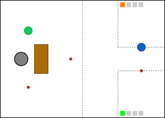
(f) (f) Blue robot successfully delivers Tool-0 to workshop-0.

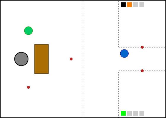
(g) (g) Blue robot runs Get-Tool to go back table. Human-0 finishes subtask-0 and starts to do subtask-1.

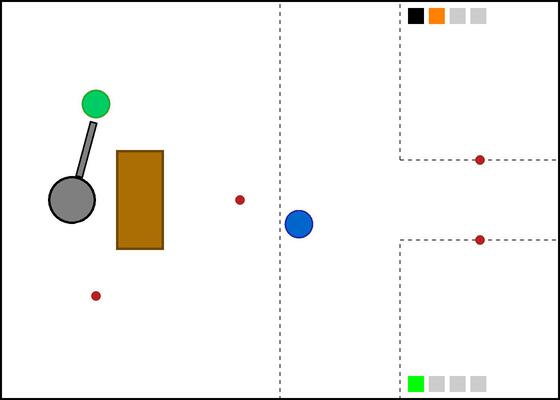
(h) (h) Arm robot executes Pass-to-M(0) to pass Tool-1 to green robot.

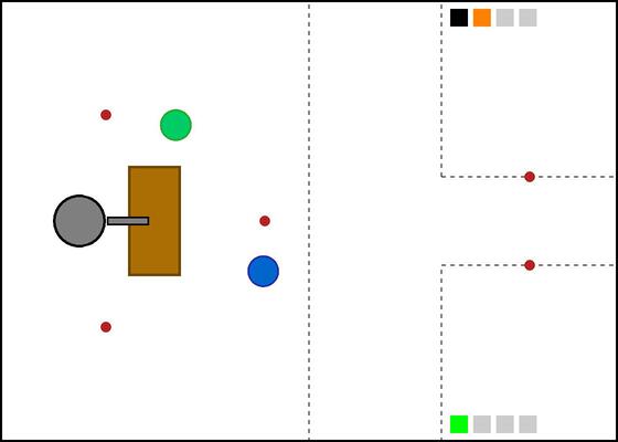
(i) (i) Arm robot runs Search-Tool(0) to find Tool-0. Green robot moves to workshop-0 by executing Go-W(0).

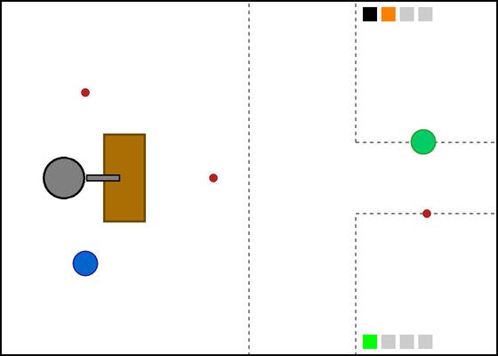
(j) (j) Green robot successfully delivers Tool-1 to workshop-0.

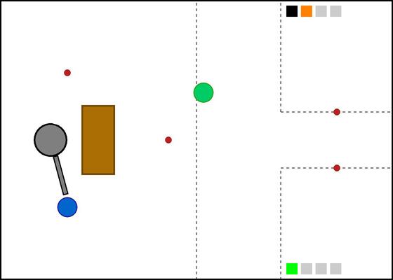
(k) (k) Arm robot executes Pass-to-M(1) to pass Tool-0 to blue robot. Green robot runs Get-Tool to go back table.

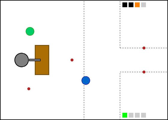
(l) (l) Arm robot runs Search-Tool(2) to find Tool-2. Blue robot moves to workshop-1 by executing Go-W(1). Human-0 finishes subtask-1 and starts to do subtask-2.

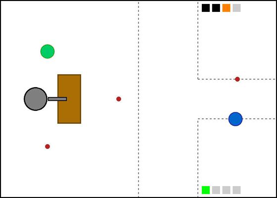
(a) (m) Blue robot successfully delivers Tool-0 to workshop-1.

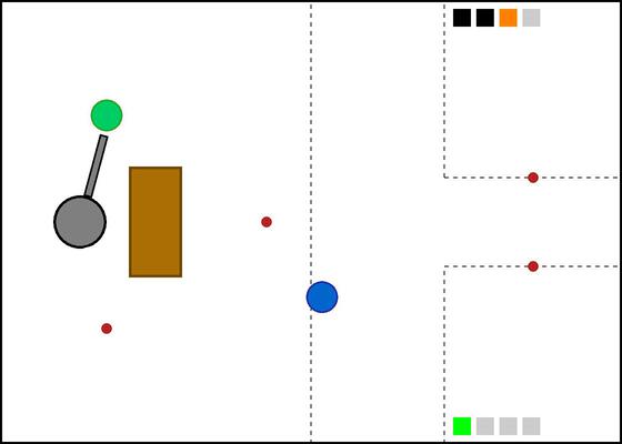
(b) (n) Arm robot executes Pass-to-M(0) to pass Tool-2 to green robot. Blue robot runs Get-Tool to go back table.

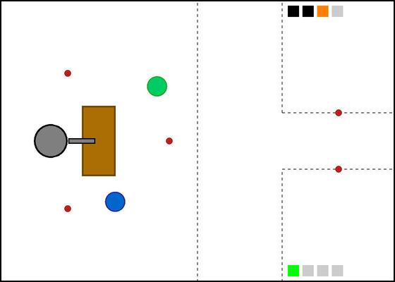
(c) (o) Arm robot runs Search-Tool(1) to find Tool-1. Green robot moves to workshop-0 by executing Go-W(0).

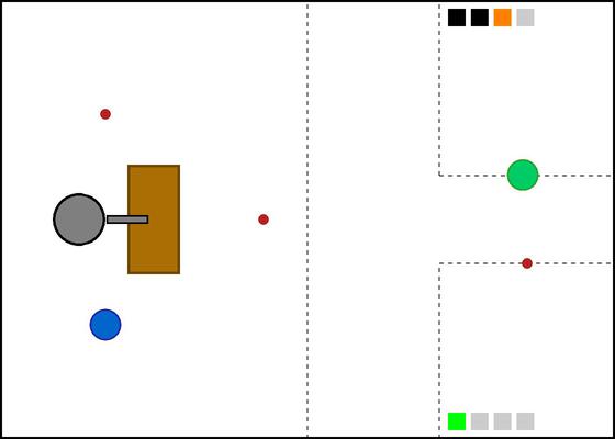
(d) (p) Green robot successfully delivers Tool-2 to workshop-0.

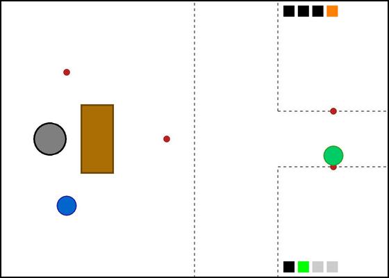
(e) (q) Green robot moves to workshop-1 by executing Go-W(1) to observe human-1’s status. Human-0 finishes subtask-2 and starts to do subtask-3.

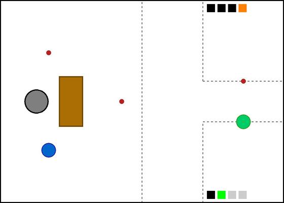
(f) (r) Green robot reaches workshop-1.

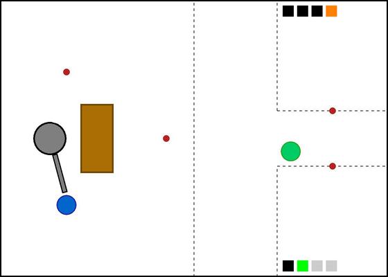
(g) (s) Arm robot executes Pass-to-M(1) to pass Tool-1 to blue robot. Green robot runs Get-Tool to go back table.

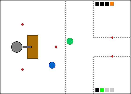
(h) (t) Arm robot runs Search-Tool(2) to find Tool-2. Blue robot moves to workshop-1 by executing Go-W(1).

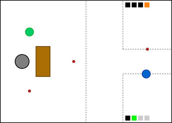
(i) (u) Blue robot successfully delivers Tool-1 to workshop-1.

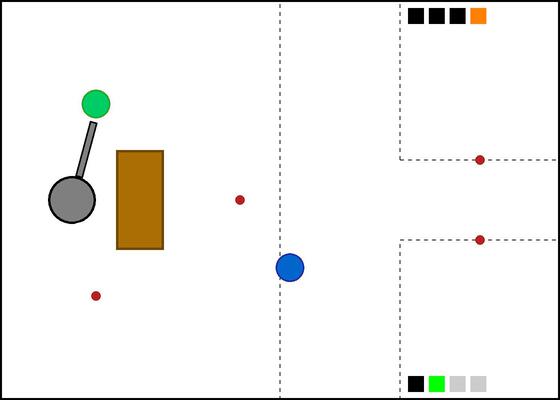
(j) (v) Blue robot runs Get-Tool to go back table. Arm robot executes Pass-to-M(0) to pass Tool-2 to green robot. Blue robot runs Get-Tool to go back table.

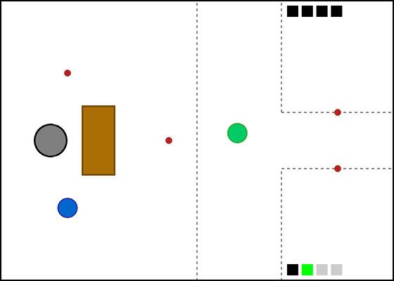
(k) (w) Green robot moves to workshop-1 by executing Go-W(1).

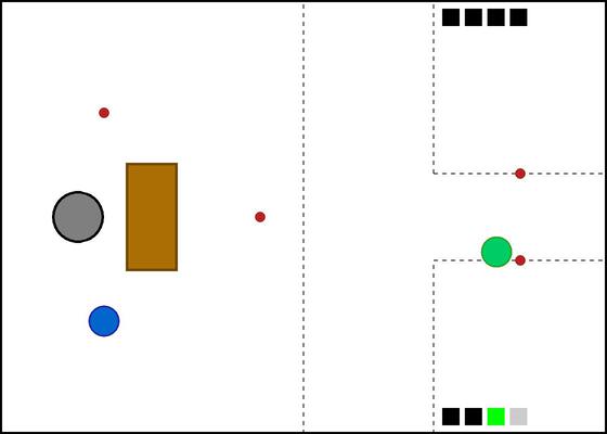
(l) (x) Human-1 finishes subtask-1 and start to do subtask-2.

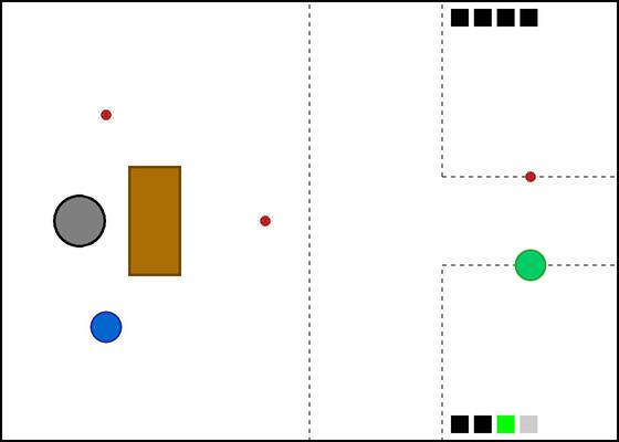
(m) (y) Green robot successfully delivers Tool-2 to workshop-1. Humans have received all tools, and for robots, the task is done.

References

- Baker et al. [2020] Bowen Baker, Ingmar Kanitscheider, Todor Markov, Yi Wu, Glenn Powell, Bob McGrew, and Igor Mordatch. Emergent tool use from multi-agent autocurricula. In Proceedings of the International Conference on Learning Representations, 2020.
- Du et al. [2019] Yali Du, Lei Han, Meng Fang, Tianhong Dai, Ji Liu, and Dacheng Tao. Liir: Learning individual intrinsic reward in multi-agent reinforcement learning. In Proceedings of the Conference on Neural Information Processing Systems, 2019.
- Foerster et al. [2018] Jakob Foerster, Gregory Farquhar, Triantafyllos Afouras, Nantas Nardelli, and Shimon Whiteson. Counterfactual multi-agent policy gradients. In Proceedings of the AAAI Conference on Artificial Intelligence, February 2018.
- Du et al. [2021] Yali Du, Bo Liu, Vincent Moens, Ziqi Liu, Zhicheng Ren, Jun Wang, Xu Chen, and Haifeng Zhang. Learning correlated communication topology in multi-agent reinforcement learning. In Proceedings of the International Conference on Autonomous Agents and Multiagent Systems, pages 456–464, 2021.
- Iqbal and Sha [2019] Shariq Iqbal and Fei Sha. Actor-attention-critic for multi-agent reinforcement learning. In Proceedings of the International Conference on Machine Learning, volume 97, pages 2961–2970, 2019.
- Li et al. [2019] Shihui Li, Yi Wu, Xinyue Cui, Honghua Dong, Fei Fang, and Stuart Russell. Robust multi-agent reinforcement learning via minimax deep deterministic policy gradient. Proceedings of the AAAI Conference on Artificial Intelligence, 33:4213–4220, 07 2019.
- Lowe et al. [2017] Ryan Lowe, Yi Wu, Aviv Tamar, Jean Harb, Pieter Abbeel, and Igor Mordatch. Multi-agent actor-critic for mixed cooperative-competitive environments. Proceedings of the Conference on Neural Information Processing Systems, 2017.
- Su et al. [2021] Jianyu Su, Stephen Adams, and Peter A Beling. Value-decomposition multi-agent actor-critics. In Proceedings of the AAAI Conference on Artificial Intelligence, 2021.
- Vinyals et al. [2019] Oriol Vinyals, Igor Babuschkin, Wojciech M. Czarnecki, Michaël Mathieu, Andrew Dudzik, Junyoung Chung, David H. Choi, Richard Powell, Timo Ewalds, Petko Georgiev, Junhyuk Oh, Dan Horgan, Manuel Kroiss, Ivo Danihelka, Aja Huang, Laurent Sifre, Trevor Cai, John P. Agapiou, Max Jaderberg, Alexander Sasha Vezhnevets, Rémi Leblond, Tobias Pohlen, Valentin Dalibard, David Budden, Yury Sulsky, James Molloy, Tom Le Paine, Çaglar Gülçehre, Ziyu Wang, Tobias Pfaff, Yuhuai Wu, Roman Ring, Dani Yogatama, Dario Wünsch, Katrina McKinney, Oliver Smith, Tom Schaul, Timothy P. Lillicrap, Koray Kavukcuoglu, Demis Hassabis, Chris Apps, and David Silver. Grandmaster level in starcraft II using multi-agent reinforcement learning. Nature., 575(7782):350–354, 2019.
- Wang et al. [2020a] Jianhong Wang, Yuan Zhang, Tae-Kyun Kim, and Yunjie Gu. Shapley q-value: A local reward approach to solve global reward games. In Proceedings of the AAAI Conference on Artificial Intelligence, 2020a.
- Wang et al. [2021a] Yihan Wang, Beining Han, Tonghan Wang, Heng Dong, and Chongjie Zhang. DOP: Off-policy multi-agent decomposed policy gradients. In Proceedings of the International Conference on Learning Representations, 2021a.
- Yang et al. [2020a] Jiachen Yang, Alireza Nakhaei, David Isele, Kikuo Fujimura, and Hongyuan Zha. Cm3: Cooperative multi-goal multi-stage multi-agent reinforcement learning. In Proceedings of the International Conference on Learning Representations, 2020a.
- Zhou et al. [2020] Meng Zhou, Ziyu Liu, Pengwei Sui, Yixuan Li, and Yuk Ying Chung. Learning implicit credit assignment for cooperative multi-agent reinforcement learning. In Proceedings of the Conference on Neural Information Processing Systems, 2020.
- Dalal et al. [2021] Murtaza Dalal, Deepak Pathak, and Ruslan Salakhutdinov. Accelerating robotic reinforcement learning via parameterized action primitives. In Proceedings of the Conference on Neural Information Processing Systems, 2021.
- Stulp and Schaal [2011] Freek Stulp and Stefan Schaal. Hierarchical reinforcement learning with movement primitives. In 11th IEEE-RAS International Conference on Humanoid Robots, 2011.
- Konidaris et al. [2011] George Dimitri Konidaris, Scott Kuindersma, Roderic A. Grupen, and Andrew G. Barto. Autonomous skill acquisition on a mobile manipulator. In Wolfram Burgard and Dan Roth, editors, Proceedings of the AAAI Conference on Artificial Intelligence, 2011.
- Konidaris et al. [2018] George Dimitri Konidaris, Leslie Pack Kaelbling, and Tomás Lozano-Pérez. From skills to symbols: Learning symbolic representations for abstract high-level planning. Journal of Artificial Intelligence Research, 61:215–289, 2018.
- Wu et al. [2020] Jimmy Wu, Xingyuan Sun, Andy Zeng, Shuran Song, Johnny Lee, Szymon Rusinkiewicz, and Thomas Funkhouser. Spatial action maps for mobile manipulation. In Proceedings of the Robotics: Science and Systems Conference, 2020.
- He et al. [2010] Ruijie He, Abraham Bachrach, and Nicholas Roy. Efficient planning under uncertainty for a target-tracking micro-aerial vehicle. In Proceedings of the International Conference on Robotics and Automation, 2010.
- Hsiao et al. [2010] Kaijen Hsiao, Leslie Pack Kaelbling, and Tomas Lozano-Perez. Task-driven tactile exploration. In Proceedings of the Robotics: Science and Systems Conference, 2010.
- Lee et al. [2021] Yiyuan Lee, Panpan Cai, and David Hsu. MAGIC: learning macro-actions for online POMDP planning. In Proceedings of the Robotics: Science and Systems Conference, 2021.
- Theocharous and Kaelbling [2004] Georgios Theocharous and Leslie Kaelbling. Approximate planning in pomdps with macro-actions. In Advances in Neural Information Processing Systems, 2004.
- Amato et al. [2014] Christopher Amato, George D. Konidaris, and Leslie P. Kaelbling. Planning with macro-actions in decentralized POMDPs. In Proceedings of the International Conference on Autonomous Agents and Multiagent Systems, 2014.
- Amato et al. [2019] Christopher Amato, George Konidaris, Leslie Pack Kaelbling, and Jonathan P. How. Modeling and planning with macro-actions in decentralized pomdps. Journal of Artificial Intelligence Research, 64:817–859, 2019.
- Amato et al. [2015a] Christopher Amato, George D. Konidaris, Ariel Anders, Gabriel Cruz, Jonathan P. How, and Leslie P. Kaelbling. Policy search for multi-robot coordination under uncertainty. In Proceedings of the Robotics: Science and Systems Conference, 2015a.
- Amato et al. [2015b] Christopher Amato, George D. Konidaris, Gabriel Cruz, Christopher A. Maynor, Jonathan P. How, and Leslie P. Kaelbling. Planning for decentralized control of multiple robots under uncertainty. In Proceedings of the International Conference on Robotics and Automation, pages 1241–1248, 2015b.
- Hoang et al. [2018] Trong Nghia Hoang, Yuchen Xiao, Kavinayan Sivakumar, Christopher Amato, and Jonathan How. Near-optimal adversarial policy switching for decentralized asynchronous multi-agent systems. In Proceedings of the International Conference on Robotics and Automation, 2018.
- Omidshafiei et al. [2016] Shayegan Omidshafiei, Ali-akbar Agha-mohammadi, Christopher Amato, Shih-Yuan Liu, Jonathan P. How, and John Vian. Graph-based cross entropy method for solving multi-robot decentralized POMDPs. In Proceedings of the International Conference on Robotics and Automation, 2016.
- Omidshafiei et al. [2017a] Shayegan Omidshafiei, Ali-akbar Agha-mohammadi, Christopher Amato, and Jonathan P. How. Decentralized control of multi-robot partially observable markov decision processes using belief space macro-actions. The International Journal of Robotics Research, 36(2):231–258, 2017a.
- de Witt et al. [2019] Christian Schroeder de Witt, Jakob Foerster, Gregory Farquhar, Philip H. S. Torr, Wendelin Boehmer, and Shimon Whiteson. Multi-agent common knowledge reinforcement learning. In Proceedings of the Conference on Neural Information Processing Systems, 2019.
- Han et al. [2019] Dongge Han, Wendelin Böhmer, Michael J. Wooldridge, and Alex Rogers. Multi-agent hierarchical reinforcement learning with dynamic termination. In PRICAI (2), volume 11671 of Lecture Notes in Computer Science, pages 80–92. Springer, 2019.
- Nachum et al. [2019] Ofir Nachum, Michael Ahn, Hugo Ponte, Shixiang Shane Gu, and Vikash Kumar. Multi-agent manipulation via locomotion using hierarchical sim2real. In Proceedings of the Conference on Robot Learning, 2019.
- Wang et al. [2020b] Rose E. Wang, J. Chase Kew, Dennis Lee, Tsang-Wei Edward Lee, Tingnan Zhang, Brian Ichter, Jie Tan, and Aleksandra Faust. Model-based reinforcement learning for decentralized multiagent rendezvous. In Proceedings of the Conference on Robot Learning, 2020b.
- Wang et al. [2021b] Tonghan Wang, Tarun Gupta, Anuj Mahajan, Bei Peng, Shimon Whiteson, and Chongjie Zhang. Rode: Learning roles to decompose multi-agent tasks. In Proceedings of the International Conference on Learning Representations, 2021b.
- Xu et al. [2021] Zhiwei Xu, Yunpeng Bai, Bin Zhang, Dapeng Li, and Guoliang Fan. HAVEN: hierarchical cooperative multi-agent reinforcement learning with dual coordination mechanism. arXiv preprint, abs/2110.07246, 2021.
- Yang et al. [2020b] Jiachen Yang, Igor Borovikov, and Hongyuan Zha. Hierarchical cooperative multi-agent reinforcement learning with skill discovery. In Proceedings of the International Conference on Autonomous Agents and Multiagent Systems, 2020b.
- Chakravorty et al. [2019] Jhelum Chakravorty, Patrick Nadeem Ward, Julien Roy, Maxime Chevalier-Boisvert, Sumana Basu, Andrei Lupu, and Doina Precup. Option-critic in cooperative multi-agent systems. arXiv preprint, arXiv:1911.12825, 2019.
- Menda et al. [2019] Kunal Menda, Yi-Chun Chen, Justin Grana, James W. Bono, Brendan D. Tracey, Mykel J. Kochenderfer, and David H. Wolpert. Deep reinforcement learning for event-driven multi-agent decision processes. IEEE Trans. Intell. Transp. Syst., 20(4):1259–1268, 2019.
- Xiao et al. [2019] Yuchen Xiao, Joshua Hoffman, and Christopher Amato. Macro-action-based deep multi-agent reinforcement learning. In Proceedings of the Conference on Robot Learning, 2019.
- Wu et al. [2021a] Jimmy Wu, Xingyuan Sun, Andy Zeng, Shuran Song, Szymon Rusinkiewicz, and Thomas Funkhouser. Spatial intention maps for multi-agent mobile manipulation. In Proceedings of the International Conference on Robotics and Automation, 2021a.
- Kraemer and Banerjee [2016] Landon Kraemer and Bikramjit Banerjee. Multi-agent reinforcement learning as a rehearsal for decentralized planning. Neurocomputing, 190:82–94, 2016.
- Oliehoek et al. [2008] Frans A. Oliehoek, Matthijs T. J. Spaan, and Nikos A. Vlassis. Optimal and approximate q-value functions for decentralized pomdps. Journal of Artificial Intelligence Research, 32:289–353, 2008.
- Wu et al. [2021b] Sarah A. Wu, Rose E. Wang, James A. Evans, Joshua B. Tenenbaum, David C. Parkes, and Max Kleiman-Weiner. Too many cooks: Coordinating multi-agent collaboration through inverse planning. Topics in Cognitive Science, 2021b.
- Sutton et al. [1999] R.S. Sutton, D. Precup, and S. Singh. Between MDPs and semi-MDPs: A framework for temporal abstraction in reinforcement learning. Artificial Intelligence, 112:181–211, 1999.
- Sutton et al. [2000] Richard S Sutton, David A McAllester, Satinder P Singh, and Yishay Mansour. Policy gradient methods for reinforcement learning with function approximation. In Advances in neural information processing systems, pages 1057–1063, 2000.
- Hausknecht and Stone [2015] Matthew Hausknecht and Peter Stone. Deep recurrent q-learning for partially observable mdps. In AAAI Fall Symposium on Sequential Decision Making for Intelligent Agents (AAAI-SDMIA15), 2015.
- Konda and Tsitsiklis [2000] Vijay R Konda and John N Tsitsiklis. Actor-critic algorithms. In Proceedings of the Conference on Neural Information Processing Systems, pages 1008–1014, 2000.
- Sutton [1988] Richard S. Sutton. Learning to predict by the methods of temporal differences. Mach. Learn., 3:9–44, 1988.
- Weaver and Tao [2001] Lex Weaver and Nigel Tao. The optimal reward baseline for gradient-based reinforcement learning. In Proceedings of the Conference on Uncertainty in Artificial Intelligence, pages 538–545. Morgan Kaufmann, 2001.
- Lyu et al. [2021] Xueguang Lyu, Yuchen Xiao, Brett Daley, and Christopher Amato. Contrasting centralized and decentralized critics in multi-agent reinforcement learning. In Proceedings of the International Conference on Autonomous Agents and Multiagent Systems, 2021.
- Alon and Zhou [2020] Yoav Alon and Huiyu Zhou. Multi-agent reinforcement learning for unmanned aerial vehicle coordination by multi-critic policy gradient optimization. IEEE Transactions on Robotics, 2020.
- Khan et al. [2019] Arbaaz Khan, Ekaterina I. Tolstaya, Alejandro Ribeiro, and Vijay Kumar. Graph policy gradients for large scale robot control. 2019.
- Mitchell et al. [2020] Rupert Mitchell, Jenny Fletcher, Jacopo Panerati, and Amanda Prorok. Multi-vehicle mixed reality reinforcement learning for autonomous multi-lane driving. In Proceedings of the International Conference on Autonomous Agents and Multiagent Systems, 2020.
- Park et al. [2020] Jin-Soo Park, Brian Tsang, Harel Yedidsion, Garrett Warnell, Daehyun Kyoung, and Peter Stone. Learning to improve multi-robot hallway navigation. In Proceedings of the Conference on Robot Learning, November 2020.
- Stone et al. [2005] Peter Stone, Richard S. Sutton, and Gregory Kuhlmann. Reinforcement learning for RoboCup-soccer keepaway. Adaptive Behavior, 2005.
- Strickland et al. [2019] Caroline Strickland, David Churchill, and Andrew Vardy. A reinforcement learning approach to multi-robot planar construction. In Proceedings of IEEE International Symposium on Multi-Robot and Multi-Agent Systems, 2019.
- Tang [2019] Yichuan Charlie Tang. Towards learning multi-agent negotiations via self-play. In Autonomous Driving Workshop, IEEE International Conference on Computer Vision, 2019.
- Chen [2014] Yu Fan Chen. Hierarchical decomposition of multi-agent markov decision processes with application to health aware planning. Master’s thesis, Massachusetts Institute of Technology, 2014.
- Luo et al. [2018] S. Luo, J. Kim, R. Parasuraman, J. H. Bae, E. T. Matson, and B. C. Min. Multi-robot rendezvous based on bearing-aided hierarchical tracking of network topology. Ad Hoc Networks, 2018.
- Oliehoek and Visser [2006] Frans A. Oliehoek and Arnoud Visser. A hierarchical model for decentralized fighting of large scale urban fires. In Proceedings of the AAMAS Workshop on Hierarchical Autonomous Agents and Multi-Agent Systems, 2006.
- Omidshafiei et al. [2017b] Shayegan Omidshafiei, Shih-Yuan Liu, Michael Everett, Brett T Lopez, Christopher Amato, Miao Liu, Jonathan P How, and John Vian. Semantic-level decentralized multi-robot decision-making using probabilistic macro-observations. In Proceedings of the International Conference on Robotics and Automation, pages 871–878, 2017b.
- Zhang et al. [2017] Shiqi Zhang, Yuqian Jiang, Guni Sharon, and Peter Stone. Multirobot symbolic planning under temporal uncertainty. In Proceedings of the 16th International Conference on Autonomous Agents and Multiagent Sytems (AAMAS), 2017.
- Yang et al. [2021] Tianpei Yang, Weixun Wang, Hongyao Tang, Jianye Hao, Zhaopeng Meng, Hangyu Mao, Dong Li, Wulong Liu, Chengwei Zhang, Yujing Hu, Yingfeng Chen, and Changjie Fan. An efficient transfer learining framework for multiagent reinforcement learining. In Proceedings of the Conference on Neural Information Processing Systems, 2021.
- Ahilan and Dayan [2019] Sanjeevan Ahilan and Peter Dayan. Feudal multi-agent hierarchies for cooperative reinforcement learning. arXiv preprint, abs/1901.08492, 2019.
- Vezhnevets et al. [2020] Alexander Sasha Vezhnevets, Yuhuai Wu, Remi Leblond, and Joel Z. Leibo. Options as responses: Grounding behavioural hierarchies in multi-agent rl. In Proceedings of the International Conference on Machine Learning, 2020.
- Mnih et al. [2015] Volodymyr Mnih, Koray Kavukcuoglu, David Silver, Andrei A. Rusu, Joel Veness, Marc G. Bellemare, Alex Graves, Martin Riedmiller, Andreas K. Fidjeland, Georg Ostrovski, Stig Petersen, Charles Beattie, Amir Sadik, Ioannis Antonoglou, Helen King, Dharshan Kumaran, Daan Wierstra, Shane Legg, and Demis Hassabis. Human-level control through deep reinforcement learning. Nature, 518:529–533, 2015.
- Bacon et al. [2017] Pierre-Luc Bacon, Jean Harb, and OPTdoina Precup. The option-critic architecture. In Proceedings of the AAAI Conference on Artificial Intelligence, pages 1726–1734, 2017.
- Maxime and Julien [2020] Chevalier-Boisvert Maxime and Roy Julien. Teamgrid, 2020. URL https://github.com/mila-iqia/teamgrid.
- Cho et al. [2014] Kyunghyun Cho, Bart van Merrienboer, Çaglar Gülçehre, Dzmitry Bahdanau, Fethi Bougares, Holger Schwenk, and Yoshua Bengio. Learning phrase representations using RNN encoder-decoder for statistical machine translation. In Empirical Methods in Natural Language Processing EMNLP, pages 1724–1734, 2014.
- Wise et al. [2016] Melonee Wise, Michael Ferguson, Derek King, Eric Diehr, and David Dymesich. Fetch & freight : Standard platforms for service robot applications. In Workshop on Autonomous Mobile Service Robots, International Joint Conference on Artificial Intelligence, 2016.
- Koubaa et al. [2016] Anis Koubaa, Mohamed-Foued Sriti, Yasir Javed, Maram Alajlan, Basit Qureshi, Fatma Ellouze, and Abdelrahman Mahmoud. Turtlebot at office: A service-oriented software architecture for personal assistant robots using ros. 2016 International Conference on Autonomous Robot Systems and Competitions (ICARSC), pages 270–276, 2016.
- Calli et al. [2015] B. Calli, A. Walsman, A. Singh, S. Srinivasa, P. Abbeel, and A. M. Dollar. Benchmarking in manipulation research: Using the Yale-CMU-Berkeley object and model set. IEEE Robotics Automation Magazine, 22(3):36–52, 2015.
- Marder-Eppstein et al. [2010] Eitan Marder-Eppstein, Eric Berger, Tully Foote, Brian Gerkey, and Kurt Konolige. The office marathon: Robust navigation in an indoor office environment. In Proceedings of the International Conference on Robotics and Automation, 2010.
- Gualtieri et al. [2018] Marcus Gualtieri, Andreas ten Pas, and Ondrej Biza. Pointcloudspython, 2018. URL https://github.com/mgualti/PointCloudsPython.
- [75] David Coleman, Ioan A. \textcommabelowSucan, Sachin Chitta, and Nikolaus Correll. Reducing the barrier to entry of complex robotic software: a moveit! case study. Journal of Software Engineering for Robotics.
- Diankov and Kuffner [2008] Rosen Diankov and James Kuffner. Openrave: A planning architecture for autonomous robotics. Technical report, 2008.
- Şucan et al. [2012] Ioan A. Şucan, Mark Moll, and Lydia E. Kavraki. The Open Motion Planning Library. IEEE Robotics & Automation Magazine, 19(4):72–82, December 2012.