Probing the non-standard neutrino interactions using quantum statistics

Abstract

Using the well established principles of Lorentz invariance, CP and CPT symmetry, and quantum statistics we do a model-independent study of effects of possible non-standard couplings of (Dirac and Majorana) neutrinos. The study is sensitive to the different quantum statistical properties of the Dirac and Majorana neutrinos which, contrary to neutrino-mediated processes of lepton number violation, could lead to observable effects not suppressed by the small ratios of neutrino and heavier particle masses. For processes with a neutrino-antineutrino pair of the same flavor in the final state, we formulate the “Dirac Majorana confusion theorem (DMCT)” showing why it is normally very difficult to observe the different behaviour of both kinds of neutrinos in experiments if they have only the standard model (SM)-like left-handed vector couplings to gauge bosons. We discuss deviations from the confusion theorem in the presence of non-standard neutrino interactions, allowing to discover or constrain such novel couplings. We illustrate the general results with two chosen examples of neutral current processes, $Z\to\nu\,\overline{\nu}$ and $\mathcal{P}_{i}\to\mathcal{P}_{f}\,\nu\,\overline{\nu}$ (with $\mathcal{P}_{i,f}$ denoting pseudoscalar mesons, such as $B,K,\pi$). Our analysis shows that using 3-body decays the presence of non-standard interactions can not only be constrained but one can also distinguish between Dirac and Majorana neutrino possibilities.

1 Introduction

Observations of neutrino oscillation Fukuda:1998mi ; Ahmad:2002jz have established the fact that neutrinos have non-zero but tiny masses and the flavor neutrinos ($\nu_{\ell}$ with $\ell=e,\mu,\tau$), which only participate in the weak interactions, are linear combinations of mass eigenstates ($\nu_{i}$ with $i=1,2,3$ having masses $m_{i}$),

$$\left\lvert\nu_{\ell}\right\rangle=\sum_{i}U_{\ell i}^{*}\left\lvert\nu_{i}\right\rangle,$$ (1)

where $U$ denotes the unitary $3\times 3$ lepton mixing matrix, also called the PMNS matrix Maki:1962mu ; Pontecorvo:1967fh . At present ParticleDataGroup:2020ssz , we know neither the values of the individual masses of the neutrinos nor the mechanism that gives rise to these tiny masses (see Refs. deGouvea:2016qpx ; Cai:2017jrq for recent reviews of various neutrino mass models). In the Standard Model of particle physics (SM) neutrinos are massless and get produced via weak interaction such that all neutrinos are left-handed and all antineutrinos are right-handed. However, as the neutrinos are not massless, handedness is not a good quantum number for neutrinos, i.e. in a frame moving faster than the neutrino (or antineutrino) the handedness will be reversed. Nevertheless, direct production of right-handed neutrinos and left-handed antineutrinos has not yet been observed in any experiment, consistent with the SM allowed $V-A$ interactions. Therefore, it is currently unknown whether the right-handed neutrinos have the same mass as the left-handed neutrinos or not. Most certainly, detection of the right-handed neutrinos and the left-handed antineutrinos would require invoking some sort of new physics (NP) which we currently do not know. To complicate the matter further, neutrinos being devoid of any electric or colour charge are the only known fermions which can possibly be their own antiparticles, i.e. they can be Majorana fermions Majorana:1937vz ; Racah:1937qq ; Furry:1938zz unlike all the others which are Dirac fermions. In most of the interesting mass models for neutrinos, all of which involve different NP setups, the Majorana nature is assumed. Like with many other aspects of neutrinos, this is yet to be decisively decided by experiments.

Various methodologies that have been proposed to probe the Majorana nature of neutrinos can be broadly grouped into the following two categories, depending on the type of process being considered.

1. Propagator probes or neutrino mediated probes: Well known examples of such processes are neutrinoless double-beta decay ($0\nu\beta\beta$) Avignone:2007fu , neutrinoless double-electron capture Blaum:2020ogl , neutrinoless muon ($\mu^{-}$) to positron ($e^{+}$) conversion Pontecorvo:1967fh ; Lee:2021hnx , $\nu$ exchange force ($\nu$ Casimir force) Grifols:1996fk ; Ferrer:1998ju ; Segarra:2020rah ; Costantino:2020bei ; Ghosh:2019dmi ; Bolton:2020xsm ; Xu:2021daf ; Ghosh:2022nzo or lepton number violating massive sterile neutrino exchange Cvetic:2010rw , which involve one or more neutrino(s) and/or antineutrino(s) as propagator(s). The lepton number violating processes involve helicity flip and are, therefore, always proportional to the unknown mass of the propagating Majorana neutrino. In addition, all the nuclear processes explored as propagator probes to infer the nature of sub-eV active neutrinos suffer from large theoretical uncertainty in the nuclear matrix elements. Although $0\nu\beta\beta$ searches have thus far not yielded any signal CUORE:2021mvw , the experimental searches for it are going on. Nevertheless, the associated issues mentioned above underline the importance of alternative methods.

2. Initial / final state probes: These involve one (or more) neutrino(s) and/or antineutrino(s) in the initial state or the final state. Some previously explored processes under this category are the neutrino-electron elastic scattering Kayser:1981nw ; Rosen:1982pj ; Dass:1984qc ; Rodejohann:2017vup , neutrino-nucleon scattering Kayser:1981nw , neutrino-nuclei scattering Millar:2018hkv , 2-body processes $\gamma^{*}\to\nu\,\overline{\nu}$ Kayser:1982br that try to explore the electromagnetic properties of neutrinos Schechter:1981hw , $Z\to\nu\,\overline{\nu}$ Shrock:1982jh , $e^{+}\,e^{-}\to\nu\,\overline{\nu}$ Ma:1989jpa , 3-body processes $K^{+}\to\pi^{+}\,\nu\,\overline{\nu}$ Nieves:1985ir , $e^{+}\,e^{-}\to\gamma\,\nu\,\overline{\nu}$ Chhabra:1992be , $e\,\gamma\to e\,\nu\,\overline{\nu}$ Berryman:2018qxn , radiative emission of neutrino pair Yoshimura:2013wva , and 4-body $B$ meson decay $B^{0}\to\mu^{+}\,\mu^{-}\,\nu_{\mu}\,\overline{\nu}_{\mu}$ Kim:2021dyj . In contrast with the propagator probes which essentially directly test the Majorana mass term, the initial/final state probes try to examine the quantum mechanical identicalness of Majorana neutrino and antineutrino via quantum statistics.

   Unlike the neutrino mass suppressed processes for propagator probes, the initial/final state probes involve SM allowed processes and therefore can be produced relatively easily in experiments. The challenge in probing the Dirac or Majorana nature of neutrinos using such probes is to infer the momenta or energies of the missing neutrinos which is always experimentally challenging.

The quantum statistics of Majorana neutrino and antineutrino stems from their quantum mechanical identical nature, and it is an intrinsic property of the Majorana neutrino just like its spin and charge. For a final state containing a pair of Majorana neutrino and antineutrino of the same flavor, the Fermi-Dirac statistics asserts that the corresponding transition amplitude is always anti-symmetrized with respect to their exchange. This anti-symmetrization does not depend on the size of the mass of neutrino ($m_{\nu}$). Therefore, there is no reason a priori to think that the difference between Dirac and Majorana neutrinos via such initial/final state probes would necessarily be dependent on $m_{\nu}$, a result that apparently (but not necessarily) contradicts the “practical Dirac Majorana confusion theorem” (DMCT) Kayser:1981nw ; Kayser:1982br . A brief overview of the literature, in this context, comparing two-body decays, three-body decays as well as four-body decays is given in Ref. Kim:2021dyj .

The various initial/final state probes can, in general, be related to one another via crossing symmetry Rosen:1982pj . For ease of discussion and without loosing any generality we concentrate in this paper on providing a generalised framework for final state probes, i.e. using processes in which a pair of neutrino and antineutrino would appear in the final state. Furthermore, we relax the helicity considerations, i.e. we do not confine ourselves to left-handed neutrinos and right-handed antineutrinos alone, since the involved interactions will take care of the helicities by default. Unlike considering only SM allowed interactions as done in Ref. Kim:2021dyj here we consider NP effects in a model-independent manner and point out their effects as well.

Before providing the layout of our paper, we would like to emphasise that the active neutrinos and antineutrinos in all the final states considered in this paper are invisible. In many NP models it is possible to have other invisible particles such as the heavy sterile neutrinos, dark matter particles or some long-lived light particles (e.g. axion-like) that decays outside the detector volume. Therefore, observation of decays into invisible states with rates modified comparing to the SM predictions usually is not sufficient by itself to determine the source of the modification, being it different types of neutrinos or entirely novel particles. The analysis we present in this paper is limited by the assumptions that neutrinos are only invisible final state but it is still useful for several reasons.

• If new invisible particles are massive (even relatively light but with masses significantly exceeding neutrino masses), they could have noticeable effects such as significant reduction in phase space, or presence of some resonance peaks corresponding to on-shell production of the long-lived particles. Corresponding modifications of visible final state particle spectra could help in distinguishing such cases from the neutrino production. Such possibilities are well explored in the literature, see e.g. Goudzovski:2022vbt for a recent detailed review of invisible $K$ meson decays in various SM extensions such as the 2-body decay $K\to\pi\,X_{\textrm{inv}}$ where the invisible particle $X_{\textrm{inv}}$ could be a Higgs mixed scalar, dark photon, or axion-like particle.

• Current experiments are in general in agreement with the SM predictions, therefore the bounds on non-standard neutrino couplings which we discuss in the paper come from comparing their effects with the size of experimental errors of relevant observables. If there are more invisible states in a given NP model, even very light ones, barring fine tuning they compete with neutrino interactions in saturating the errors, tightening the bounds. Thus the limits on NP neutrino couplings which we discuss can be considered as (again barring fine tuning and potential cancellations) being on the conservative side.

• Finally, in many SM extensions neutrinos remain the only ultra-light and weakly interacting (thus “invisible”) particles. In such cases methodology proposed in the paper can be directly used to constrain NP neutrino couplings for a chosen BSM model.

Our paper is organised as follows. Following Introduction, in section 2 we present a model-independent general formalism for processes involving a neutrino and antineutrino pair of the same flavor in the final state and we provide a generalised statement of DMCT in context of these processes. In section 3 we discuss how the effects of quantum statistics and symmetry properties of transition amplitudes can be utilised to probe NP interactions in neutrino sector and potentially lead to substantial difference between Dirac and Majorana neutrinos. In the following section 4 we illustrate the general results with two suitably chosen two-body and three-body neutral current decays, showing how the bounds on the NP couplings depend on the assumed neutrino nature. The possibility of distinguishing the Dirac and Majorana neutrinos by measuring the visible particles energy spectrum in the three-body decays is discussed in section 5. Finally we conclude in section 6 highlighting the various salient aspects of our study.

2 Model-independent formalism for processes containing $\boldsymbol{\nu\,\overline{\nu}}$ in the final state

2.1 Choice of process

Let us consider a general process with a neutrino and an antineutrino of the same flavor in the final state, say

$$X(p_{X})\to Y(p_{Y})\,\nu(p_{1})\,\overline{\nu}(p_{2}),$$

where $X,Y$ can be single or multi-particle states, $Y$ can also be null, the contents of $X$ and $Y$ (if it exists) can only be any visible particle and the 4-momenta $p_{X},p_{Y}$ are assumed to be well measured so that one can unambiguously infer the total missing 4-momentum of $\nu\,\overline{\nu}$, $p_{\textrm{miss}}=p_{1}+p_{2}$. So the 4-momentum of $X$ must either be fixed by design of the experiment (e.g. $X$ might be a particle produced at rest in the laboratory or be the constituent of a collimated beam of known energy or it could consist of two colliding particles of known 4-momenta) or the 4-momentum of $X$ be inferred from the fully-tagged partner particle with which it is pair-produced. The final state $Y$ should not contain any additional neutrinos or antineutrinos. The process could be a decay or scattering depending on whether $X$ is a single particle state or two particle state. Some actual processes that satisfy such criteria are $e^{+}\,e^{-}\to\nu\,\overline{\nu}$, $Z\to\nu\,\overline{\nu}$, $e^{+}\,e^{-}\to\gamma\,\nu\,\overline{\nu}$, $K\to\pi\,\nu\,\overline{\nu}$, $B\to K\,\nu\,\overline{\nu}$, $B^{0}\to\mu^{+}\,\mu^{-}\,\nu_{\mu}\,\overline{\nu}_{\mu}$, $J/\psi\to\mu^{+}\,\mu^{-}\,\nu_{\mu}\,\overline{\nu}_{\mu}$, $H\to\tau^{+}\,\tau^{-}\,\nu_{\tau}\,\overline{\nu}_{\tau}$ etc.

Schematically the process $X\to Y\,\nu\,\overline{\nu}$ is drawn in Fig. 1. Since Majorana neutrino and antineutrino are quantum mechanically identical, there is an additional diagram with exchanged 4-momenta $p_{1}\leftrightarrow p_{2}$ in the Majorana case as shown in Fig. 1. The effect of this exchange diagram in Majorana case can, in many instances but not always, be absorbed into a single diagram like the one for the Dirac case but with a different effective vertex. In section 4 we shall encounter a few examples where the effective vertex for Majorana case is different from Dirac case. An example process where we can not absorb the direct and exchange diagram contributions to the effective vertex factor is $B^{0}\to\mu^{+}\,\mu^{-}\,\nu_{\mu}\,\overline{\nu}_{\mu}$ as discussed in Ref. Kim:2021dyj .

Additionally, it should be noted that in this work we assume that in any of the processes under our consideration, the effect of measurements should not destroy the identical nature of Majorana neutrino and antineutrino. This is akin to putting the constrain that in a double-slit experiment meant to observe the interference of light, no measurement should identify through which slit the photon has passed.

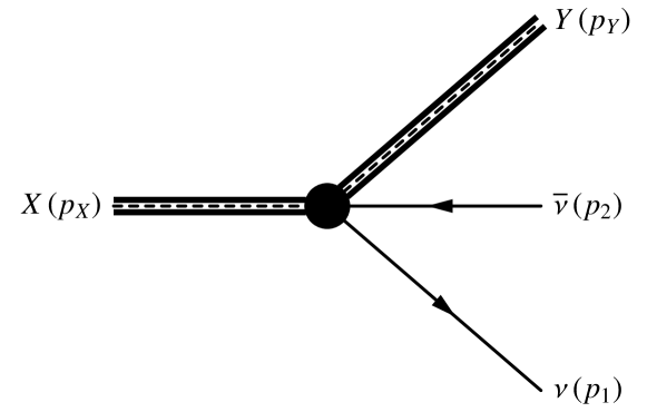
(a) Dirac neutrinos

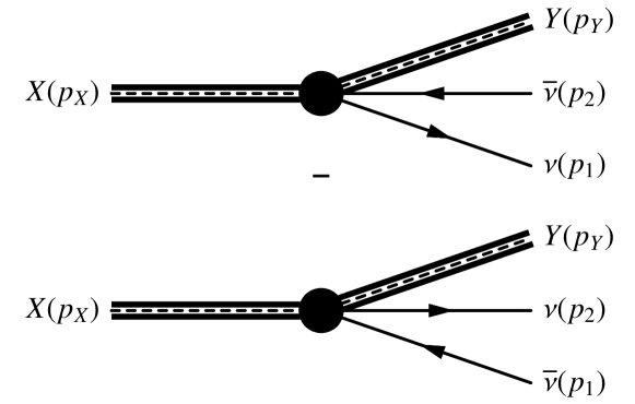
(b) Majorana neutrinos (with exchange diagram)

Figure 1: A cartoon (pseudo-Feynman diagrams) for the processes $X\to Y\,\nu\,\overline{\nu}$, with both Dirac and Majorana neutrino possibilities. The blob in these diagrams represents the effective vertex and it includes both SM and NP contributions. Although Majorana antineutrino is indistinguishable from Majorana neutrino, we keep using the notation of $\overline{\nu}$ for antineutrino and $\nu$ for neutrino simply as a book-keeping device.

2.2 Origin of observable difference between Dirac and Majorana neutrinos

The transition amplitude is, in general, dependent on all the 4-momenta of participating particles. For brevity of expression and without loss of generality, we denote the transition amplitude by only mentioning the $p_{1}$, $p_{2}$ dependence. For Dirac neutrinos, the transition amplitude can be written as,

$$\mathscr{M}^{D}=\mathscr{M}(p_{1},p_{2}),$$ (2)

while for Majorana case the amplitude is anti-symmetrized with respect to the exchange of the Majorana neutrino and antineutrino which are quantum mechanically identical fermions,

$$\mathscr{M}^{M}=\dfrac{1}{\sqrt{2}}\Big{(}\underbrace{\mathscr{M}(p_{1},p_{2})}_{\textrm{Direct amplitude}}-\underbrace{\mathscr{M}(p_{2},p_{1})}_{\textrm{Exchange amplitude}}\Big{)},$$ (3)

where $1/\sqrt{2}$ takes care of the symmetry factor. Note that the amplitudes of Eqs. (2) and (3) do not necessarily assume SM interactions, they can involve NP effects as well, and hence they include the most general structures of the amplitude that are allowed by Lorentz invariance. A general analysis that specifically exploits the symmetry properties of the amplitude in context of generic NP possibilities is given in Sec. 3.

The difference between Dirac and Majorana cases that can possibly be probed is obtained after squaring the amplitudes and taking their difference, which is given by,

$$\left|\mathscr{M}^{D}\right|^{2}-\left|\mathscr{M}^{M}\right|^{2} =\frac{1}{2}\Bigg{(}\underbrace{\left|\mathscr{M}(p_{1},p_{2})\right|^{2}}_{\textrm{Direct term}}-\underbrace{\left|\mathscr{M}(p_{2},p_{1})\right|^{2}}_{\textrm{Exchange term}}\Bigg{)}$$

$$\quad+\underbrace{\textrm{Re}\left(\mathscr{M}(p_{1},p_{2})^{*}\,\mathscr{M}(p_{2},p_{1})\right)}_{\textrm{Interference term}}.$$ (4)

From Eq. (4) it is easy to conclude that there are essentially two sources of difference between Dirac and Majorana cases,

1. unequal contributions from “Direct term” and “Exchange term”, i.e.

   $$\underbrace{\left|\mathscr{M}(p_{1},p_{2})\right|^{2}}_{\textrm{Direct term}}\neq\underbrace{\left|\mathscr{M}(p_{2},p_{1})\right|^{2}}_{\textrm{Exchange term}},$$ (5)

2. non-zero contribution from the “Interference term”, i.e.

   $$\underbrace{\textrm{Re}\left(\mathscr{M}(p_{1},p_{2})^{*}\,\mathscr{M}(p_{2},p_{1})\right)}_{\textrm{Interference term}}\neq 0.$$ (6)

However, note that in the case when no individual information about $\nu\,\overline{\nu}$ are either known or deducible, the only difference between Dirac and Majorana cases that can be experimentally accessed is obtained after full integration over $p_{1}$ and $p_{2}$ which gives,

$$\iint\left(\left|\mathscr{M}^{D}\right|^{2}-\left|\mathscr{M}^{M}\right|^{2}\right)\mathrm{d}^{4}p_{1}\,\mathrm{d}^{4}p_{2}$$

$$=\iint\underbrace{\textrm{Re}\left(\mathscr{M}(p_{1},p_{2})^{*}\,\mathscr{M}(p_{2},p_{1})\right)}_{\textrm{Interference term}}\mathrm{d}^{4}p_{1}\,\mathrm{d}^{4}p_{2},$$ (7)

where we have used the fact that although, in general, the “Direct” and “Exchange” terms may differ, when we fully integrate over the 4-momenta of neutrino and antineutrino we do get

$$\iint\underbrace{\left|\mathscr{M}(p_{1},p_{2})\right|^{2}}_{\textrm{Direct term}}\mathrm{d}^{4}p_{1}\,\mathrm{d}^{4}p_{2}=\iint\underbrace{\left|\mathscr{M}(p_{2},p_{1})\right|^{2}}_{\textrm{Exchange term}}\mathrm{d}^{4}p_{1}\,\mathrm{d}^{4}p_{2},$$ (8)

as $p_{1}$ and $p_{2}$ act as dummy variables in this case.

2.3 “Dirac-Majorana Confusion Theorem” for the neutrino interactions in the SM

In most of the experimental scenarios, especially true for processes of the form $X\to Y\,\nu\,\overline{\nu}$, information about individual neutrino momenta is not available. In such a case the difference between the Dirac and the Majorana neutrinos is given only by the integrated interference term in Eq. (7). If we further consider only SM interactions without any NP contributions, then the $V-A$ interaction of SM would always produce left-handed neutrino and right-handed antineutrino, even if the mass of the neutrino and antineutrino is considered to be non-zero. In such a case the evaluation of the squared Feynman diagram for the “Interference term” would, in general, necessarily involve two helicity flips which would make it proportional to $m_{\nu}^{2}$, i.e.

$$\underbrace{\textrm{Re}\left(\mathscr{M}^{\textrm{SM}}(p_{1},p_{2})^{*}\,\mathscr{M}^{\textrm{SM}}(p_{2},p_{1})\right)}_{\textrm{Interference term in the SM}}\propto m_{\nu}^{2}.$$

Thus, if only SM interactions are considered and one fully integrates over the neutrino and antineutrino 4-momenta, the difference between Dirac and Majorana cases would be proportional to $m_{\nu}^{2}$. This can be considered as a generalised statement of the “practical Dirac Majorana confusion theorem” (DMCT).

The above statement still holds taking into account that in many cases experiments can measure the total 4-momentum of the neutrino and antineutrino pair in the final state, $p_{1}+p_{2}$, equal to the difference between initial and final 4-momenta of the visible particles. The knowledge of $p_{1}+p_{2}$ only (not $p_{1}$ and $p_{2}$ individually), gives access to that part of the full phase space for the neutrino pair which is obviously symmetric under the exchange $p_{1}\leftrightarrow p_{2}$. Thus argument about symmetric integration and corresponding cancellation between “Direct” and “Exchange” terms in Eq. (8) still holds, even if the phase space integral is not done over the full range of $p_{1},p_{2}$. In such a scenario, all the cross sections or decay rate distributions expressed in terms of parameters related to the 4-momenta of visible particles will always be identical if pure SM interactions are assumed (up to the neutrino mass suppressed effects). However, as we will show in the following sections, the distributions of visible particles may differ if one also allows non-standard neutrino interactions.

The remaining possibility of experimental observation of the difference between the Dirac and Majorana neutrinos in the SM is to reconstruct or at least constrain the neutrino 4-momenta or some of their components such as the energies, so that full integration over the neutrino and antineutrino 4-momenta is not necessary and one can directly use Eq. (4), without worrying about the cancellation in Eq. (8). This, in general, is difficult as neutrinos are invisible in detectors and their 4-momenta can be only inferred from the kinematics of visible particles. Still, it may be possible for some particular configuration(s) of them, however occurring only for a small fraction of all kinematically allowed final states.

Relevant example of such “special” kinematic scenario has been proposed in Ref. Kim:2021dyj , where authors consider the 4-body decay of the form $X\to y_{1}\,y_{2}\,\nu\,\overline{\nu}$ with $y_{1}$ and $y_{2}$ flying away back-to-back with equal magnitudes of 3-momenta in the rest frame of $X$. In such case, the $\nu$ and $\overline{\nu}$ also fly away back-to-back with equal energies $E_{\nu}=(m_{X}-E_{y_{1}}-E_{y_{2}})/2$, where $E_{y_{1}}$, $E_{y_{2}}$ denote the energies of $y_{1}$ and $y_{2}$ respectively and $m_{X}$ is the mass of parent particle $X$. This is discussed in detail in Ref. Kim:2021dyj taking the example of $B^{0}\to\mu^{-}\,\mu^{+}\,\nu_{\mu}\,\overline{\nu}_{\mu}$. As the authors point out, other meson decays such as those of neutral $K$, or $D$, or $J/\psi$, or $\Upsilon(n\textrm{S})$ decays as well as Higgs decays might also be useful for such studies. The difference between Dirac and Majorana cases does not necessarily depend on the size of the neutrino mass, and hence might be feasible to discover in future experiments.

3 New Physics scenarios and practical DMCT

There is no reason a priori for the “practical DMCT” to hold, if NP contributions in the neutrino interactions are allowed, as in this case Eq. (4) “Direct” and “Exchange” terms in general do not need to cancel each other. To illustrate it more clearly using symmetry properties of the transition amplitude, let us assume that some (yet unknown) NP at high energy modifies the low energy effective neutrino interactions we want to explore in processes of the form $X\to Y\,\nu\,\overline{\nu}$, and the SM singlet right-handed neutrinos and left-handed antineutrinos might as well participate in such interactions.

3.1 DMCT from the perspective of exchange symmetry

Although process specific analysis using exchange symmetry is found in the literature, a process-independent general analysis highlighting the difference between Dirac and Majorana neutrinos would be useful in context of NP interactions. Below we provide such an analysis.

The amplitude for $X(p_{X})\to Y(p_{Y})\,\nu(p_{1})\,\overline{\nu}(p_{2})$ for Majorana neutrinos must be still anti-symmetric with respect to the 4-momentum exchange $p_{1}\leftrightarrow p_{2}$, as was noted in Eq. (3). The Dirac amplitude of Eq. (2) could, in principle, be split into two parts, one symmetric and the other anti-symmetric under the exchange $p_{1}\leftrightarrow p_{2}$, i.e.

$$\mathscr{M}^{D}=\mathscr{M}(p_{1},p_{2})=\mathscr{M}_{\textrm{symm}}(p_{1},p_{2})+\mathscr{M}_{\textrm{anti-symm}}(p_{1},p_{2}),$$ (9)

where by definition we have

$$\mathscr{M}_{\textrm{symm}}(p_{1},p_{2}) =\frac{1}{2}\Big{(}\mathscr{M}(p_{1},p_{2})+\mathscr{M}(p_{2},p_{1})\Big{)}$$

$$=\mathscr{M}_{\textrm{symm}}(p_{2},p_{1}),$$ (10a)

$$\mathscr{M}_{\textrm{anti-symm}}(p_{1},p_{2}) =\frac{1}{2}\Big{(}\mathscr{M}(p_{1},p_{2})-\mathscr{M}(p_{2},p_{1})\Big{)}$$

$$=-\,\mathscr{M}_{\textrm{anti-symm}}(p_{2},p_{1}),$$ (10b)

so that the Majorana amplitude of Eq. (3) is automatically given by,

$$\mathscr{M}^{M}=\sqrt{2}\,\mathscr{M}_{\textrm{anti-symm}}(p_{1},p_{2}).$$ (11)

With the decomposition of amplitudes as shown in Eqs. (9) and (11), the difference between Dirac and Majorana neutrinos is given by,

$$\left|\mathscr{M}^{D}\right|^{2}-\left|\mathscr{M}^{M}\right|^{2} =\left|\mathscr{M}_{\textrm{symm}}(p_{1},p_{2})+\mathscr{M}_{\textrm{anti-symm}}(p_{1},p_{2})\right|^{2}$$

$$\quad-2\left|\mathscr{M}_{\textrm{anti-symm}}(p_{1},p_{2})\right|^{2}\,,$$

$$=\left|\mathscr{M}_{\textrm{symm}}(p_{1},p_{2})\right|^{2}-\left|\mathscr{M}_{\textrm{anti-symm}}(p_{1},p_{2})\right|^{2}$$

$$\quad+2\,\textrm{Re}\left(\mathscr{M}_{\textrm{symm}}(p_{1},p_{2})^{*}\,\mathscr{M}_{\textrm{anti-symm}}(p_{1},p_{2})\right)\,.$$ (12)

If one were to do full integration over the neutrino and antineutrino 4-momenta, the interference term in Eq. (12) vanishes as it is anti-symmetric under the $p_{1}\leftrightarrow p_{2}$ exchange and one is left with

$$\iint\left(\left|\mathscr{M}^{D}\right|^{2}-\left|\mathscr{M}^{M}\right|^{2}\right)\mathrm{d}^{4}p_{1}\,\mathrm{d}^{4}p_{2}$$

$$= \iint\left(\left|\mathscr{M}_{\textrm{symm}}(p_{1},p_{2})\right|^{2}-\left|\mathscr{M}_{\textrm{anti-symm}}(p_{1},p_{2})\right|^{2}\right)\mathrm{d}^{4}p_{1}\,\mathrm{d}^{4}p_{2},$$ (13)

which does not necessarily vanish in presence of NP interactions. Note that Eqs. (7) and (13) are equivalent to one another, but Eq. (13) highlights the symmetry properties that were not explicitly evident in Eq. (7).

3.2 Processes with $\boldsymbol{\nu\,\overline{\nu}}$ produced via neutral current interactions

As an example, let us consider NP effects on neutrino-antineutrino neutral current interactions. In such a case, the amplitude would have the generic form,

$$\mathscr{M}(p_{1},p_{2})=\sum_{i}\mathcal{S}_{i}\,\Big{[}\overline{u}(p_{1})\,\Gamma_{i}\,\varv(p_{2})\Big{]},$$

where $\mathcal{S}_{i}$ denotes the parts of the amplitude which do not depend on $p_{1}$ and $p_{2}$ or contain algebraic expressions such as $(p_{1}+p_{2})^{2}$ which are symmetric under $p_{1}\leftrightarrow p_{2}$ exchange, and $\Gamma_{i}$ could be $\mathbf{1}$, $\gamma^{5}$, $\gamma^{\alpha}$, $\gamma^{\alpha}\,\gamma^{5}$, $\sigma^{\alpha\beta}$ or $\sigma^{\alpha\beta}\,\gamma^{5}$, which respectively correspond to scalar, pseudo-scalar, vector, axial-vector, tensor and axial-tensor interactions. For Majorana neutrinos it is well known that $\overline{u}(p_{1})\,\Gamma\,\varv(p_{2})=-\,\overline{u}(p_{2})\,C\,\Gamma^{T}\,C^{-1}\,\varv(p_{1})$ Denner:1992vza where $C$ denotes the charge conjugation operator. Using this it is easy to show that $\mathscr{M}_{\textrm{symm}}(p_{1},p_{2})$ gets contributions only from vector, tensor and axial-tensor interactions while $\mathscr{M}_{\textrm{anti-symm}}(p_{1},p_{2})$ gets contributions from scalar, pseudo-scalar and axial-vector interactions alone, i.e.

$$\mathscr{M}(p_{1},p_{2}) =\sum_{i}\mathcal{S}_{i}\,\Big{[}\overline{u}(p_{1})\,\Gamma_{i}\,\varv(p_{2})\Big{]}$$

$$=\begin{cases}\mathscr{M}_{\textrm{symm}}(p_{1},p_{2})&\text{ for }\Gamma_{i}=\gamma^{\alpha},\,\sigma^{\alpha\beta},\,\sigma^{\alpha\beta}\,\gamma^{5},\\ \mathscr{M}_{\textrm{anti-symm}}(p_{1},p_{2})&\text{ for }\Gamma_{i}=\mathbf{1},\,\gamma^{5},\,\gamma^{\alpha}\,\gamma^{5}.\end{cases}$$

Therefore, the NP effects could lead to observable differences between the Dirac and Majorana neutrino interactions, even after integrating over the unknown neutrino and antineutrino 4-momenta, if the symmetric and anti-symmetric parts of the amplitude do not cancel either due to some imposed symmetry (like in the case of vector $V-A$ interactions in the SM) or due to some accidental fine-tuning and numerical cancellation between different types of couplings. In section 4 we illustrate the general considerations presented above discussing a chosen physical process of the form $X\to Y\,\nu\,\overline{\nu}$.

4 Example 2-body and 3-body neutral current decays with $\boldsymbol{\nu\,\overline{\nu}}$ in the final state

To illustrate the results arising from the general formalism presented in previous sections, we study here in detail two example processes, in both cases assuming the non-vanishing NP effects, namely the 2-body decay of $Z^{0}$ boson, $Z\to\nu_{\ell}\,\overline{\nu}_{\ell}$ and the 3-body decay of an initial pseudo-scalar meson to a final pseudo-scalar meson and $\nu\,\overline{\nu}$. A recent model-independent analysis of 3-body leptonic decays, but in context of heavy sterile neutrinos and facilitated by charged current interaction, can be found in Ref. Marquez:2022bpg .

4.1 2-body decay of $\boldsymbol{Z\to\nu_{\ell}\,\overline{\nu}_{\ell}}$

Considering Lorentz invariance alone, it is possible to write down the most general $Z(p)\to\nu(p_{1})\,\overline{\nu}(p_{2})$ decay amplitude as follows (for Dirac neutrinos),

$$\mathscr{M}^{D} =-i\,\epsilon_{\alpha}(p)\,\overline{u}(p_{1})\,\Big{[}\Big{(}g_{S}^{+}+g_{P}^{+}\,\gamma^{5}\Big{)}\,p^{\alpha}+\Big{(}g_{S}^{-}+g_{P}^{-}\,\gamma^{5}\Big{)}\,q^{\alpha}$$

$$\hskip 65.44133pt+\gamma^{\alpha}\Big{(}g_{V}+g_{A}\,\gamma^{5}\Big{)}+\sigma^{\alpha\beta}\Big{(}g_{T_{\textrm{md}}}^{+}+g_{T_{\textrm{ed}}}^{+}\gamma^{5}\Big{)}\,p_{\beta}$$

$$\hskip 65.44133pt+\sigma^{\alpha\beta}\Big{(}g_{T_{\textrm{md}}}^{-}+g_{T_{\textrm{ed}}}^{-}\gamma^{5}\Big{)}\,q_{\beta}\Big{]}\,\varv(p_{2}),$$ (14)

where $\epsilon_{\alpha}(p)$ denotes the polarisation 4-vector of $Z$, $q=p_{1}-p_{2}$, $p=p_{1}+p_{2}$, $g_{X}^{(\pm)}$ with $X=S,P,V,A,T_{\textrm{md}},T_{\textrm{ed}}$ denote the various possible coupling constants corresponding to scalar, pseudo-scalar, vector, axial-vector, tensor (magnetic dipole) and axial-tensor (electric dipole) kind of interactions. In the SM, $g_{S}^{\pm}=g_{P}^{\pm}=g_{T_{\textrm{md}}}^{\pm}=g_{T_{\textrm{ed}}}^{\pm}=0$ and $g_{V}=-g_{A}=\dfrac{g_{Z}}{4}$ where $g_{Z}=e/(\sin\theta_{W}\,\cos\theta_{W})$ with $\theta_{W}$ being the weak mixing angle and $e$ being the electric charge of positron. In presence of NP all the above coupling constants could, in principle, differ from the SM values. Noting that all terms proportional to $p^{\alpha}$ vanish since $p^{\alpha}\,\epsilon_{\alpha}(p)=0$, and utilising Gordon identities as well as neglecting terms proportional to $m_{\nu}$, the tensorial components get eliminated to yield,

$$\mathscr{M}^{D}=-i\,\epsilon_{\alpha}(p)\,\overline{u}(p_{1})\,\Big{[}\Big{(}g_{S}+g_{P}\,\gamma^{5}\Big{)}\,q^{\alpha}+\gamma^{\alpha}\Big{(}g_{V}+g_{A}\,\gamma^{5}\Big{)}\Big{]}\,\varv(p_{2}),$$ (15)

where $g_{S}=g_{S}^{-}+i\,g_{T_{\textrm{md}}}^{+}$ and $g_{P}=g_{P}^{-}+i\,g_{T_{\textrm{ed}}}^{+}$. Further, if we consider CP and CPT conservation in the decay $Z\to\nu_{\ell}\,\overline{\nu}_{\ell}$, $g_{S}=0$ and $g_{P}=0$ ought to be satisfied respectively. This implies, only vector and axial-vector couplings are allowed. The most general expression for the decay amplitude for $Z\to\nu_{\ell}\,\overline{\nu}_{\ell}$ with Dirac neutrinos is given by,

$$\mathscr{M}^{D}=\mathscr{M}(p_{1},p_{2})=-\frac{i\,g_{Z}}{2}\upepsilon_{\alpha}(p)\,\left[\overline{u}(p_{1})\,\gamma^{\alpha}\left(C_{V}^{\ell}-C_{A}^{\ell}\,\gamma^{5}\right)\,\varv(p_{2})\right],$$ (16)

where, to keep our analysis more general, we have elevated the parameters $g_{V}$ and $g_{A}$ to possibly be different for every the lepton family by adding the superscript $\ell=e,\mu,\tau$ such that the vector and axial-vector couplings are expressed as $g_{V}^{\ell}=\dfrac{g_{Z}}{2}C_{V}^{\ell}$ and $g_{A}^{\ell}=-\dfrac{g_{Z}}{2}C_{A}^{\ell}$ respectively, with

$$C_{V,A}^{\ell}=\frac{1}{2}+\varepsilon_{V,A}^{\ell},$$ (17)

where $\varepsilon_{V}^{\ell}$, $\varepsilon_{A}^{\ell}$ parameterise the NP effects, vanishing in the SM case. The amplitude for Majorana case is given by

$$\mathscr{M}^{M} =\dfrac{1}{\sqrt{2}}\Big{(}\mathscr{M}(p_{1},p_{2})-\mathscr{M}(p_{2},p_{1})\Big{)}$$

$$=\frac{i\,g_{Z}\,C_{A}^{\ell}}{\sqrt{2}}\upepsilon_{\alpha}(p)\,\left[\overline{u}(p_{1})\,\gamma^{\alpha}\,\gamma^{5}\,\varv(p_{2})\right].$$ (18)

It is clear that we can combine the direct and exchange amplitudes in this case and effectively redefine the vertex structure for $Z\to\nu_{\ell}\,\overline{\nu}_{\ell}$ when Majorana neutrinos are considered.

Keeping neutrino mass dependent terms in the amplitude squares, we get different results for Dirac and Majorana neutrinos:

$$\left|\mathscr{M}^{D}\right|^{2} =\frac{g_{Z}^{2}}{3}\Bigg{(}\left((C_{V}^{\ell})^{2}+(C_{A}^{\ell})^{2}\right)\left(m_{Z}^{2}-m_{\nu}^{2}\right)$$

$$\hskip 56.9055pt+3\left((C_{V}^{\ell})^{2}-(C_{A}^{\ell})^{2}\right)m_{\nu}^{2}\Bigg{)},$$ (19)

$$\left|\mathscr{M}^{M}\right|^{2} =\frac{2\,g_{Z}^{2}\,(C_{A}^{\ell})^{2}}{3}\left(m_{Z}^{2}-4\,m_{\nu}^{2}\right),$$ (20)

such that

$$\left|\mathscr{M}^{D}\right|^{2}-\left|\mathscr{M}^{M}\right|^{2} =\frac{g_{Z}^{2}}{3}\bigg{(}\left((C_{V}^{\ell})^{2}-(C_{A}^{\ell})^{2}\right)\left(m_{Z}^{2}+2\,m_{\nu}^{2}\right)$$

$$\hskip 28.45274pt+6\,(C_{A}^{\ell})^{2}\,m_{\nu}^{2}\bigg{)}$$

$$=\begin{cases}\dfrac{g_{Z}^{2}}{2}m_{\nu}^{2},&\left(\parbox[c]{56.9055pt}{\centering for SM alone\@add@centering}\right)\\[14.22636pt] \dfrac{g_{Z}^{2}}{3}\left(\varepsilon_{V}^{\ell}-\varepsilon_{A}^{\ell}\right)m_{Z}^{2},&\left(\parbox[c]{56.9055pt}{\centering with NP but neglecting $m_{\nu}$\@add@centering}\right)\end{cases}$$ (21)

where we have kept only the leading order contributions of $\varepsilon_{V,A}^{\ell}$ while considering NP effects. It is clear that the SM result is fully in agreement with “practical Dirac Majorana confusion theorem”. However, the difference between Dirac and Majorana neutrinos appears in context of NP contributions even when one neglects $m_{\nu}$ dependent terms (unless, of course, $\varepsilon_{V}^{\ell}=\varepsilon_{A}^{\ell}$ in which case the additional NP contributions effectively rescale the SM allowed $V-A$ coupling). Possible example of NP effects in this $Z$ boson decay could arise from kinetic mixing of $Z$ with the neutral gauge bosons from extra gauge groups like additional $U(1)$ or $SU(2)_{R}$. In this paper we are not concerned with any specific model of NP to keep our results very general.

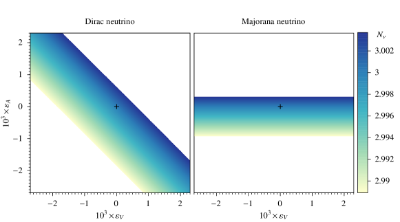
Figure 2: Constraints on the NP parameters $\varepsilon_{V}$ and $\varepsilon_{A}$ from the experimentally measured number of light neutrino species $N_{\nu}$. The point denoted by ‘$+$’ corresponds to the SM values $\varepsilon_{V}=0=\varepsilon_{A}$. In the plots here $\varepsilon_{V,A}^{2}$ contributions have not been neglected.

The decay width of $Z$ boson into invisible final states is well measured and can constrain NP contributions to neutrino couplings. Neglecting small neutrino masses, the decay rates for $Z\to\nu_{\ell}\,\overline{\nu}_{\ell}$ for Dirac and Majorana neutrino possibilities are given by

$$\Gamma^{D}(Z\to\nu_{\ell}\,\overline{\nu}_{\ell}) =\Gamma_{Z}^{0}\left(1+2\,\varepsilon_{V}^{\ell}+2\,\varepsilon_{A}^{\ell}\right),$$ (22a)

$$\Gamma^{M}(Z\to\nu_{\ell}\,\overline{\nu}_{\ell}) =\Gamma_{Z}^{0}\left(1+4\,\varepsilon_{A}^{\ell}\right),$$ (22b)

where $\Gamma_{Z}^{0}$ denotes the SM decay rate for $m_{\nu}=0$,

$$\Gamma_{Z}^{0}=\dfrac{G_{F}\,m_{Z}^{3}}{12\sqrt{2}\,\pi},$$ (23)

with $G_{F}$ being the Fermi constant. Thus, in presence of NP effects and neglecting $m_{\nu}$ dependent terms, the total invisible width of $Z$ boson is given by,

$$\Gamma_{Z,\textrm{inv}}=\begin{cases}\displaystyle\Gamma_{Z}^{0}\,\Bigg{(}3+2\sum_{\ell=e,\mu,\tau}\left(\varepsilon_{V}^{\ell}+\varepsilon_{A}^{\ell}\right)\Bigg{)},&\left(\parbox[c]{56.9055pt}{\centering for Dirac neutrinos\@add@centering}\right)\\[14.22636pt] \displaystyle\Gamma_{Z}^{0}\,\Bigg{(}3+4\sum_{\ell=e,\mu,\tau}\varepsilon_{A}^{\ell}\Bigg{)}.&\left(\parbox[c]{56.9055pt}{\centering for Majorana neutrinos\@add@centering}\right)\end{cases}$$ (24)

The ratio $\Gamma_{Z,\textrm{inv}}/\Gamma_{Z}^{0}$ is a measure of the number of light neutrino species $N_{\nu}$ and its experimental estimate is ParticleDataGroup:2020ssz ; Janot:2019oyi ,

$$N_{\nu}=\Gamma_{Z,\textrm{inv}}/\Gamma_{Z}^{0}=2.9963\pm 0.0074.$$ (25)

Using Eq. (24) in Eq. (25) we get the following constraints on the NP parameters,

$$\sum_{\ell=e,\mu,\tau}\left(\varepsilon_{V}^{\ell}+\varepsilon_{A}^{\ell}\right) =-0.0018\pm 0.0037, \left(\parbox[c]{56.9055pt}{\centering for Dirac neutrinos\@add@centering}\right)$$ (26a)

$$\sum_{\ell=e,\mu,\tau}\varepsilon_{A}^{\ell} =-0.0009\pm 0.0018, \left(\parbox[c]{56.9055pt}{\centering for Majorana neutrinos\@add@centering}\right)$$ (26b)

which are perfectly consistent with zero, however obviously different for Majorana and Dirac neutrinos. In the latter case, it is in principle even possible that deviations from the SM $V-A$-type couplings are individually larger but cancel between the vector and axial contributions.

Assuming that the NP contributions do not depend on the flavor of the neutrino, i.e. $\varepsilon_{V,A}^{e}=\varepsilon_{V,A}^{\mu}=\varepsilon_{V,A}^{\tau}\equiv\varepsilon_{V,A}$ (say), and keeping the contributions from $\varepsilon_{V,A}^{2}$ terms as well, we find that $\varepsilon_{V}$ and $\varepsilon_{A}$ get constrained by Eq. (25) as shown in Fig. 2. It is clear from Fig. 2 that the SM values $\varepsilon_{V}=0=\varepsilon_{A}$ (corresponding to the point indicated by ‘$+$’) are within the allowed $1\sigma$ region.

The results above can be interpreted in two-fold way. First, one can assume some specific NP model that affects the weak neutral current processes involving neutrinos, with well defined Lagrangian and field interactions. In this case nature of the neutrinos follows from the model construction. As always, to predict the phenomenological consequences of the given SM extension, one needs first to estimate the experimentally allowed size of NP couplings. An example above illustrates how such bounds differ for a particular decay depending on the type of neutrinos in a model. Obviously, the realistic NP models usually contain a number of new parameters and constraining them requires combining bounds from various measurements, often not only from the neutrino sector. The invisible $Z$ boson decay discussed in this section, as a quantity known to a good accuracy, should always be one of observables contributing to such more general analysis and fitting NP model to data.

Second, it may be not known in advance what is the nature of the neutrino fields, apart from the assumption that they can have interactions going beyond the SM-like $V-A$ couplings. In this case single measurement like the invisible $Z$ boson decay cannot help distinguish the type of neutrino fields if some deviations from the SM predictions are observed (or even if neutrinos are responsible for such deviations). However, again when more measurements are combined (especially for the final states with more than 2 particles, which allow to construct additional observables like shown in the next section) it may be possible to constrain individual couplings and, in an optimistic scenario, understand the nature of “invisible” sector of the theory. Again, reconstructing the model couplings must take into account the fact that it depends on the nature of neutrino fields.

Finally, apart from specific decay discussed in this section, the general formalism presented before can be applied to other 2-body neutrino decays which can be considered in searches for various channels of decays of BSM particles, e.g. new neutral heavy gauge bosons or scalars (here possible example are the sneutrino decays in R-parity violating MSSM).

4.2 3-body decay of an initial pseudo-scalar meson to a final pseudo-scalar meson and $\boldsymbol{\nu\,\overline{\nu}}$

As a second example let us consider the general decay $\mathcal{P}_{i}\to\mathcal{P}_{f}\,\nu_{\ell}\,\overline{\nu}_{\ell}$ where $\mathcal{P}_{i}$ is the parent pseudo-scalar meson with mass $M_{i}$ and $\mathcal{P}_{f}$ is the daughter pseudo-scalar meson with mass $M_{f}$. For example, $\mathcal{P}_{i}$ could be $B$ or $K$ meson, then $\mathcal{P}_{f}$ would be either $K$ or $\pi$ meson respectively.

Considering Lorentz invariance, the effective Lagrangian for $\mathcal{P}_{i}\to\mathcal{P}_{f}\,\nu_{\ell}\,\overline{\nu}_{\ell}$ decay can be written as follows,

$$\mathscr{L} =J_{SL}^{\ell}\Big{(}\overline{\psi}_{\nu}\,P_{L}\,\psi_{\overline{\nu}}\Big{)}+J_{SR}^{\ell}\Big{(}\overline{\psi}_{\nu}\,P_{R}\,\psi_{\overline{\nu}}\Big{)}$$

$$\quad+\left(J_{VL}^{\ell}\right)_{\alpha}\Big{(}\overline{\psi}_{\nu}\,\gamma^{\alpha}P_{L}\,\psi_{\overline{\nu}}\Big{)}+\left(J_{VR}^{\ell}\right)_{\alpha}\Big{(}\overline{\psi}_{\nu}\,\gamma^{\alpha}\,P_{R}\,\psi_{\overline{\nu}}\Big{)}$$

$$\quad+\left(J_{TL}^{\ell}\right)_{\alpha\beta}\Big{(}\overline{\psi}_{\nu}\,P_{L}\,\sigma^{\alpha\beta}\,\psi_{\overline{\nu}}\Big{)}+\left(J_{TR}^{\ell}\right)_{\alpha\beta}\Big{(}\overline{\psi}_{\nu}\,\sigma^{\alpha\beta}\,P_{R}\,\psi_{\overline{\nu}}\Big{)}+\textrm{h.c.},$$ (27)

where $\psi_{j}$ denotes the fermionic field of $j=\nu_{\ell},\overline{\nu}_{\ell}$ and $J_{SL}^{\ell}$, $J_{SR}^{\ell}$, $\left(J_{VL}^{\ell}\right)_{\alpha}$, $\left(J_{VR}^{\ell}\right)_{\alpha}$, $\left(J_{TL}^{\ell}\right)_{\alpha\beta}$ $\left(J_{TR}^{\ell}\right)_{\alpha\beta}$ denote the different hadronic currents describing the quark level transitions from $\mathcal{P}_{i}$ to $\mathcal{P}_{f}$ meson. We have used the superscript $\ell$ to accommodate any possible differences in the effective Lagrangian when different neutrino flavors are considered. The subscripts $S$, $V$ and $T$ in the hadronic currents denote the fact that the associated external leptonic currents are scalar, vector and tensor type, respectively, and in addition they carry also the chirality index. In the SM, at tree-level, only the $V-A$ interaction is present, while the scalar and tensor interactions involving left-handed neutrinos might be generated from quantum loops and are hence expected to be suppressed. Additionally, in the SM the right-handed neutrinos do not take part in any interaction. In this analysis we do not consider any specific NP model to keep our results general, thus in Eq. (27) we have included all possible interactions disregarding the helicity of neutrino.

The decay amplitude for $\mathcal{P}_{i}(p_{i})\to\mathcal{P}_{f}(p_{f})\,\nu_{\ell}(p_{1})\,\overline{\nu}_{\ell}(p_{2})$, considering the neutrino and the antineutrino to be Dirac fermions, is given by,

$$\mathscr{M}^{D}=\mathscr{M}(p_{1},p_{2}) =\overline{u}(p_{1})\Big{[}F_{SL}^{\ell}\,P_{L}\,+F_{SR}^{\ell}\,P_{R}$$

$$\hskip 42.67912pt+\left(F_{VL}^{\ell+}\,p_{\alpha}+F_{VL}^{\ell-}q_{\alpha}\right)\,\gamma^{\alpha}\,P_{L}$$

$$\hskip 42.67912pt+\left(F_{VR}^{\ell+}\,p_{\alpha}+F_{VR}^{\ell-}q_{\alpha}\right)\,\gamma^{\alpha}\,P_{R}\,$$

$$\hskip 42.67912pt+F_{TL}^{\ell}\,p_{\alpha}\,q_{\beta}\,\sigma^{\alpha\beta}\,P_{L}$$

$$\hskip 42.67912pt+F_{TR}^{\ell}\,p_{\alpha}\,q_{\beta}\,\sigma^{\alpha\beta}\,P_{R}\Big{]}\varv(p_{2}),$$ (28)

where $p=p_{i}+p_{f}$, $q=p_{i}-p_{f}=p_{1}+p_{2}$ and the various form factors $F_{SX}^{\ell}$, $F_{VX}^{\ell\pm}$, $F_{TX}^{\ell}$ are defined as follows,

$$\left\langle\mathcal{P}_{f}\Big{\lvert}J_{SX}^{\ell}\Big{\rvert}\mathcal{P}_{i}\right\rangle =F_{SX}^{\ell},$$ (29a)

$$\left\langle\mathcal{P}_{f}\Big{\lvert}\left(J_{VX}^{\ell}\right)_{\alpha}\Big{\rvert}\mathcal{P}_{i}\right\rangle =F_{VX}^{\ell+}\,p_{\alpha}+F_{VX}^{\ell-}\,q_{\alpha},$$ (29b)

$$\left\langle\mathcal{P}_{f}\Big{\lvert}\left(J_{TX}^{\ell}\right)_{\alpha\beta}\Big{\rvert}\mathcal{P}_{i}\right\rangle =F_{TX}^{\ell}\,p_{\alpha}\,q_{\beta},$$ (29c)

where by $X$ we denote the chirality index, $X=L,R$.

The form factors defined in Eq. (29) are complex and, in general, functions of the square of the momentum transferred, i.e. $q^{2}\equiv s$. Here the form factors also include the CKM matrix elements and their mass dimensions are different since the explicit dependencies on quark/meson masses are hidden for simplicity of expressions.

The decay amplitude for Majorana neutrinos is obtained by anti-symmetrization with respect to exchange of $p_{1}$ and $p_{2}$ and is given by,

$$\mathscr{M}^{M} =\frac{1}{\sqrt{2}}\Big{(}\mathscr{M}(p_{1},p_{2})-\mathscr{M}(p_{2},p_{1})\Big{)}$$

$$=\sqrt{2}\,\overline{u}(p_{1})\,\Bigg{[}F_{SL}^{\ell}\,P_{L}+F_{SR}^{\ell}\,P_{R}$$

$$\hskip 45.5244pt+\bigg{(}\frac{F_{VR}^{\ell+}-F_{VL}^{\ell+}}{2}\,p_{\alpha}+\frac{F_{VR}^{\ell-}-F_{VL}^{\ell-}}{2}q_{\alpha}\bigg{)}\,\gamma^{\alpha}\,\gamma^{5}\Bigg{]}\,\varv(p_{2}).$$ (30)

Once again we find that the direct and exchange amplitudes in this case can be combined to effectively redefine the vertex factors for each possible interaction. Notably, for Majorana neutrinos no vector or tensor neutral currents are possible.

Since the scalar products that appear in the amplitude squares are Lorentz invariant, they can be evaluated in any chosen frame of reference. It is well known that any 3-body decay can be fully described by two independent parameters. For simplicity we choose them as $s=\big{(}p_{1}+p_{2}\big{)}^{2}$ and the angle $\theta$ between the 3-momenta of the neutrino and the final state meson in the center-of-momentum frame of the $\nu\,\overline{\nu}$ pair, as shown in Fig. 3.

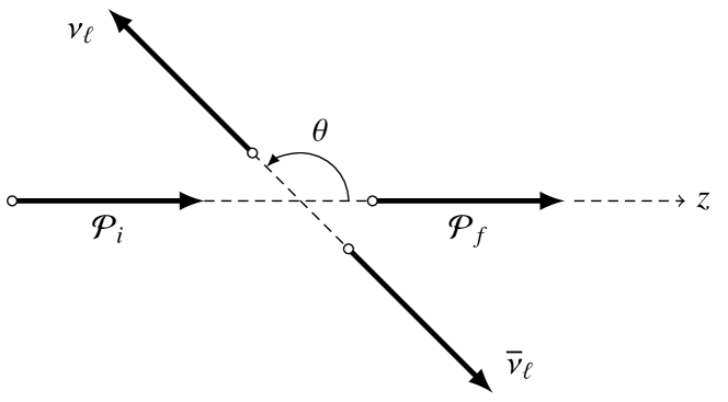
Figure 3: Kinematic configuration of the decay $\mathcal{P}_{i}\to\mathcal{P}_{f}\,\nu\,\overline{\nu}$ in center-of-momentum frame of the $\nu\,\overline{\nu}$ pair.

The amplitude squares for both Dirac and Majorana cases can be written in the following form in terms of the variables $s$ and $\cos\theta$,

$$\left\lvert\mathscr{M}^{D/M}\right\rvert^{2}=C_{0}^{D/M}+C_{1}^{D/M}\,\cos\theta+C_{2}^{D/M}\,\cos^{2}\theta,$$ (31)

where, neglecting the small terms proportional to neutrino mass $m_{\nu}$ we have,

$$C_{0}^{D} =s\,\Big{(}\left|F_{SL}^{\ell}\right|^{2}+\left|F_{SR}^{\ell}\right|^{2}\Big{)}+\lambda\,\Big{(}\left|F_{VL}^{\ell+}\right|^{2}+\left|F_{VR}^{\ell+}\right|^{2}\Big{)},$$ (32a)

$$C_{1}^{D} =2\,s\,\sqrt{\lambda}\,\left(\textrm{Im}\left(F_{SL}^{\ell}F_{TL}^{\ell*}\right)+\textrm{Im}\left(F_{SR}^{\ell}F_{TR}^{\ell*}\right)\right),$$ (32b)

$$C_{2}^{D} =-\lambda\,\Big{(}\left|F_{VL}^{\ell+}\right|^{2}+\left|F_{VR}^{\ell+}\right|^{2}-s\,\left(\left|F_{TL}^{\ell}\right|^{2}+\left|F_{TR}^{\ell}\right|^{2}\right)\Big{)},$$ (32c)

$$C_{0}^{M} =2\,s\,\Big{(}\left|F_{SL}^{\ell}\right|^{2}+\left|F_{SR}^{\ell}\right|^{2}\Big{)}+\lambda\,\left|F_{VL}^{\ell+}-F_{VR}^{\ell+}\right|^{2},$$ (32d)

$$C_{1}^{M} =0,$$ (32e)

$$C_{2}^{M} =-\lambda\,\left|F_{VL}^{\ell+}-F_{VR}^{\ell+}\right|^{2},$$ (32f)

with

$$\lambda=M_{i}^{4}+M_{f}^{4}+s^{2}-2\left(M_{i}^{2}\,M_{f}^{2}+s\,M_{i}^{2}+s\,M_{f}^{2}\right).$$ (33)

The Dirac amplitude square may contain a term odd in $\cos\theta$, while it is always absent in Majorana case. This, in principle, could be probed if the angle $\theta$ could be measured experimentally. However, at present the angle $\theta$ can not be observed as both the neutrino and antineutrino remain undetected in the detector near their point of production. In addition, such a term also requires simultaneously existence of both tensor and scalar NP interactions (in addition, with complex couplings) and is likely to be small.

The differential decay rate in the rest frame of the parent meson $\mathcal{P}_{i}$ after integration over the unobservable $\cos\theta$ is given by,

$$\frac{\mathrm{d}\Gamma^{D/M}}{\mathrm{d}s}=\frac{1}{(2\,\pi)^{3}}\frac{b}{16\,M_{i}^{3}}\left(C_{0}^{D/M}+\frac{1}{3}C_{2}^{D/M}\right),$$ (34)

where

$$b=\frac{\sqrt{\lambda}}{2}\,\sqrt{1-\frac{4\,m_{\nu}^{2}}{s}}.$$ (35)

In terms of the form factors, we get

$$\frac{\mathrm{d}\Gamma^{D}}{\mathrm{d}s} =\frac{1}{(2\,\pi)^{3}}\frac{\lambda\,b}{24\,M_{i}^{3}}\Bigg{(}\left|F_{VL}^{\ell+}\right|^{2}+\left|F_{VR}^{\ell+}\right|^{2}$$

$$\hskip 71.13188pt+\frac{3s}{2\lambda}\,\left(\left|F_{SL}^{\ell}\right|^{2}+\left|F_{SR}^{\ell}\right|^{2}\right)$$

$$\hskip 71.13188pt+\frac{s}{2}\,\left(\left|F_{TL}^{\ell}\right|^{2}+\left|F_{TR}^{\ell}\right|^{2}\right)\Bigg{)}\,,$$ (36a)

$$\frac{\mathrm{d}\Gamma^{M}}{\mathrm{d}s} =\frac{1}{(2\,\pi)^{3}}\frac{\lambda\,b}{24\,M_{i}^{3}}\Bigg{(}\left|F_{VL}^{\ell+}-F_{VR}^{\ell+}\right|^{2}+\frac{3s}{\lambda}\,\left(\left|F_{SL}^{\ell}\right|^{2}+\left|F_{SR}^{\ell}\right|^{2}\right)\Bigg{)}.$$ (36b)

From Eqs. (36a) and (36b) it is clear that the presence of additional forms of NP interactions on top of the usual SM allowed $V-A$ interaction can lead to observable differences between the Dirac and Majorana neutrinos.

To show the impact of presence of such additional non-standard interactions we consider a simple effective parametrization of NP effects (using again the chirality index $X=L,R$),

$$F_{SX}^{\ell} =M_{i}\,F_{\textrm{SM}}\,\varepsilon_{SX}^{\ell},$$ (37a)

$$F_{VL}^{\ell+} =F_{\textrm{SM}}\,\Big{(}1+\varepsilon_{VL}^{\ell}\Big{)},$$ (37b)

$$F_{VR}^{\ell+} =F_{\textrm{SM}}\,\varepsilon_{VR}^{\ell},$$ (37c)

$$F_{TX}^{\ell} =\frac{1}{M_{i}}\,F_{\textrm{SM}}\,\varepsilon_{TX}^{\ell},$$ (37d)

where $\varepsilon_{QX}^{\ell}$, $Q=S,V,T$, denote the relative size of the NP contributions with respect to the SM contribution and are assumed to be small, $\left|\varepsilon_{QX}^{\ell}\right|\ll 1$. We include $M_{i}$ factors in Eq. (37) to accommodate for the difference in mass dimensions of various form factors so as to keep the NP parameters $\varepsilon_{QX}^{\ell}$ dimensionless. Substituting Eq. (37) in Eq. (36) we obtain,

$$\frac{\mathrm{d}\Gamma^{D}}{\mathrm{d}s} =\frac{\mathrm{d}\Gamma^{\textrm{SM}}}{\mathrm{d}s}\Bigg{(}1+2\,\textrm{Re}\,\varepsilon_{VL}^{\ell}+\left|\varepsilon_{VL}^{\ell}\right|^{2}+\left|\varepsilon_{VR}^{\ell}\right|^{2}$$

$$\hskip 45.5244pt+\frac{3sM_{i}^{2}}{2\lambda}\,\left(\left|\varepsilon_{SL}^{\ell}\right|^{2}+\left|\varepsilon_{SR}^{\ell}\right|^{2}\right)$$

$$\hskip 45.5244pt+\frac{s}{2M_{i}^{2}}\,\left(\left|\varepsilon_{TL}^{\ell}\right|^{2}+\left|\varepsilon_{TR}^{\ell}\right|^{2}\right)\Bigg{)}$$

$$\approx\frac{\mathrm{d}\Gamma^{\textrm{SM}}}{\mathrm{d}s}\Bigg{(}1+2\,\textrm{Re}\,\varepsilon_{VL}^{\ell}\Bigg{)}\,,$$ (38a)

$$\frac{\mathrm{d}\Gamma^{M}}{\mathrm{d}s} =\frac{\mathrm{d}\Gamma^{\textrm{SM}}}{\mathrm{d}s}\Bigg{(}1+2\,\textrm{Re}\,\varepsilon_{VL}^{\ell}-2\,\textrm{Re}\,\varepsilon_{VR}^{\ell}+\left|\varepsilon_{VL}^{\ell}-\varepsilon_{VR}^{\ell}\right|^{2}$$

$$\hskip 45.5244pt+\frac{3sM_{i}^{2}}{\lambda}\,\left(\left|\varepsilon_{SL}^{\ell}\right|^{2}+\left|\varepsilon_{SR}^{\ell}\right|^{2}\right)\Bigg{)}$$

$$\approx\frac{\mathrm{d}\Gamma^{\textrm{SM}}}{\mathrm{d}s}\Bigg{(}1+2\,\textrm{Re}\,\varepsilon_{VL}^{\ell}-2\,\textrm{Re}\,\varepsilon_{VR}^{\ell}\Bigg{)},$$ (38b)

where we defined the SM decay rate as

$$\frac{\mathrm{d}\Gamma^{\textrm{SM}}}{\mathrm{d}s}=\frac{1}{(2\,\pi)^{3}}\frac{\lambda\,b\,\left|F_{\textrm{SM}}\right|^{2}}{24\,M_{i}^{3}}\,.$$ (39)

Therefore, the difference between Dirac and Majorana cases, to the leading order in the NP parameters, is given by,

$$\frac{\mathrm{d}\Gamma^{D}}{\mathrm{d}s}-\frac{\mathrm{d}\Gamma^{M}}{\mathrm{d}s}\approx 2\,\frac{\mathrm{d}\Gamma^{\textrm{SM}}}{\mathrm{d}s}\,\textrm{Re}\,\varepsilon_{VR}^{\ell},$$ (40)

which implies that non-zero difference can, in principle, arise only if $\textrm{Re}\,\varepsilon_{VR}^{\ell}\neq 0$.

Similar to the case of $Z\to\nu\,\overline{\nu}$ decay, only the NP contributions to the vector currents contribute to both decay rates in the lowest linear order. In addition, presence of only $\varepsilon_{VL}$, i.e. change of normalisation of the SM $V-A$ interaction, modifies the decay into Dirac neutrinos, while both $\varepsilon_{VL}$ and $\varepsilon_{VR}$ affect the expression for the Majorana neutrino decay. Scalar and tensor interactions lead to higher order corrections, quadratic in NP effects, and are likely to be small and difficult to observe taking into experimental accuracy of corresponding measurement, both current and in foreseeable future. Moreover, if only constant vector or scalar NP contributions are present, the shape of the decay spectrum $\mathrm{d}\Gamma^{D/M}/\mathrm{d}s$ is identical for Majorana and Dirac neutrinos and, therefore, when used alone it can not distinguish between the two possibilities (unless in some specific NP model both $\varepsilon_{VL}$ and $\varepsilon_{VR}$ are known and thus the difference in normalisation of the spectrum is also known). However, it is interesting to note that if tensor NP contributions are substantial enough to be observed, it would point out to the Dirac nature of neutrino, since tensor interactions do not affect the $s$ distribution for Majorana neutrinos at all. We elaborate on these aspects in Sec. 5 where we study the $s$ distributions while considering each of the possible interactions one at a time.

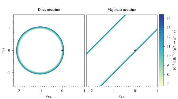
Figure 4: Constraints on the NP parameters $\varepsilon_{VL}$ and $\varepsilon_{VR}$ (assuming them to be real and including quadratic term contributions) using experimentally measured branching ratio of $K^{+}\to\pi^{+}\,\nu\,\overline{\nu}$ as given in Eq. (41). The point denoted by ‘$+$’ corresponds to the SM values $\varepsilon_{VL}=0=\varepsilon_{VR}$.

As an example of experimental constraints which can be imposed on the NP neutrino couplings by the three-body decays, let us consider the decay $K^{+}\to\pi^{+}\,\nu\,\overline{\nu}$ whose branching ratio as reported by NA62 Collaboration NA62:2021zjw is,

$$\textrm{Br}^{\textrm{Exp}}\left(K^{+}\to\pi^{+}\,\nu\,\overline{\nu}\right)=\left(\left.10.6^{+4.0}_{-3.4}\right|_{\textrm{stat}}\pm 0.9_{\textrm{syst}}\right)\times 10^{-11},$$ (41)

which is consistent with the SM prediction Buras:2015qea ,

$$\textrm{Br}^{\textrm{SM}}\left(K^{+}\to\pi^{+}\,\nu\,\overline{\nu}\right)=\left(9.11\pm 0.72\right)\times 10^{-11}.$$ (42)

Neglecting the terms quadratic in NP contributions and assuming that terms that are linear in the parameters $\varepsilon_{QX}$ are approximately constant with respect to $q^{2}\equiv s$ (which could affect the integration of $\mathrm{d}\Gamma/\mathrm{d}s$ to the total branching ratio), we get the following constraints from the above mentioned experimental measurement,

$$\sum_{\ell=e,\mu,\tau}\textrm{Re}\,\varepsilon_{VL}^{\ell} =0.082\pm 0.214,\quad\left(\parbox[c]{56.9055pt}{\centering for Dirac neutrinos\@add@centering}\right)$$ (43a)

$$\sum_{\ell=e,\mu,\tau}\left(\textrm{Re}\,\varepsilon_{VL}^{\ell}-\textrm{Re}\,\varepsilon_{VR}^{\ell}\right) =0.082\pm 0.214,\quad\left(\parbox[c]{56.9055pt}{\centering for Majorana neutrinos\@add@centering}\right)$$ (43b)

which are consistent with zero.

If we assume that only vector NP contributions are dominant and $\varepsilon_{VL}^{\ell}$, $\varepsilon_{VR}^{\ell}$ are both real and identical for all neutrino flavors, i.e. $\varepsilon_{VX}^{e}=\varepsilon_{VX}^{\mu}=\varepsilon_{VX}^{\tau}\equiv\varepsilon_{VX}$ (with $X=L,R$), then the experimental measurement of Eq. (41) constrains the NP parameters $\varepsilon_{VL}$ and $\varepsilon_{VR}$ as shown in Fig. 4 (there we have kept the quadratic terms in $\varepsilon_{VL}$, $\varepsilon_{VR}$ as well, assuming that in principle they can be large compared to the SM terms but cancel out due to some kind of accidental or symmetry-related fine-tuning). It is clear from Fig. 4 that if we allow for some amount of fine tuning and cancellations, large NP contributions are still possible in both Dirac and Majorana neutrino possibilities. One can also note that the contributions from scalar and tensor form factors are always positive, so even if they are also non-negligible, they can only tighten the bounds on $\varepsilon_{VL}$ and $\varepsilon_{VR}$ plotted in Fig. 4.

With more precise experimental decays data in future, the estimate of NP contribution will also improve. Another interesting decay in the same category as $K^{+}\to\pi^{+}\,\nu\,\overline{\nu}$ is the decay $B^{+}\to K^{+}\,\nu\,\overline{\nu}$ which is being pursued at Belle II and awaiting its branching ratio measurement. The SM prediction for the branching ratio for this decay Blake:2016olu is,

$$\textrm{Br}^{\textrm{SM}}\left(B^{+}\to K^{+}\,\nu\,\overline{\nu}\right)=\left(4.6\pm 0.5\right)\times 10^{-6},$$ (44)

while the current experimental upper limit by Belle II Belle-II:2021rof is $4.1\times 10^{-5}$ at $90\%$ confidence level.

Again, as already discussed in the previous section, constraining individual parameters of the NP model (or in the best case scenario even determining the nature of invisible sector of the theory, including distinguishing the Dirac and Majorana character of neutrinos) requires combining bounds from many measurements, in addition to the example discussed above.

5 Distinguishing Dirac and Majorana neutrinos via NP effects

Although experimentally measured branching ratios of the two- and three-body decays can only constrain the probable NP couplings of neutrinos, from Eq. (36) and the non-approximated part of Eq. (38) it seems that by analysing observed $s$ (missing mass-square) distribution in the three-body decays one can also distinguish between Dirac and Majorana neutrino possibilities, provided it can be measured with sufficient accuracy. This could be very challenging and may not possible in the near future as meson decays into neutrino pair are rare and current experimental statistics are not sufficient to probe the energy spectra of the visible final state particles (equivalent to the $s$ distribution). However, it might eventually be possible when more data get accumulated. Alternatively, similar analysis could be applied to collision experiments with the neutrino antineutrino pair in the final state, where statistics are much higher but one has to deal with significant backgrounds and related uncertainties.

As mentioned in the Introduction, one should note that modification of the spectra of the visible particle in the final state of the decay can also be caused if some invisible particles other than neutrinos are present in the final state. For distinguishing such NP possibilities, i.e. the presence of other invisible particles, we encourage the reader to follow other existing proposals such as the ones discussed in Refs. Goudzovski:2022vbt ; Kim:2018hlp . Specifically, in context of 3-body semi-hadronic decays of mesons such as $K\to\pi\,f\,\overline{f}$ where $f$ could be fermionic dark matter, heavy neutral lepton or some long-lived fermion in addition to the usual active neutrino possibility, the methods proposed in Ref. Kim:2018hlp using angular distributions and Dalitz plot asymmetries could be useful in distinguishing these NP possibilities, without worrying about hadronic uncertainties. In the discussion below, we focus only on active neutrinos as the invisible particles and study the effect of NP interactions over the experimentally observable distribution.

Before proceeding further we note that in Eq. (38), $\varepsilon_{SL}$ and $\varepsilon_{SR}$ as well as $\varepsilon_{TL}$ and $\varepsilon_{TR}$ contribute in a similar manner. Therefore, we can discuss their impact in terms of two effective NP parameters $\varepsilon_{S}$ and $\varepsilon_{T}$, defined as follows,

$$\varepsilon_{S} =\sqrt{|\varepsilon_{SL}|^{2}+|\varepsilon_{SR}|^{2}},$$ (45a)

$$\varepsilon_{T} =\sqrt{|\varepsilon_{TL}|^{2}+|\varepsilon_{TR}|^{2}}.$$ (45b)

Further we also consider, for simplicity, that all the NP parameters are real quantities and agnostic to the flavor of the neutrino in the final state. Below we shall first look at the generic trends in the various $s$ distributions for various NP possibilities without considering any specific decay, and then we show how these generic features can affect the spectrum of a specific decay, on an example chosen to be $B\to K\,\nu\,\overline{\nu}$.

5.1 The generic trends in $\boldsymbol{s}$ (missing mass-square) distributions

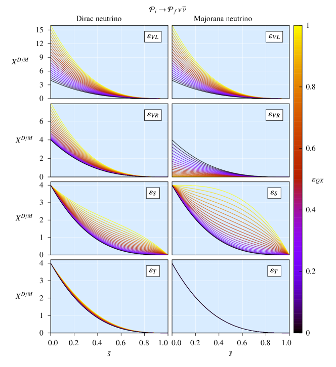
Figure 5: Comparison of various generic NP contributions in $\mathcal{P}_{i}\to\mathcal{P}_{f}\,\nu_{\ell}\,\overline{\nu}_{\ell}$ decay assuming that the mass of the final meson $\mathcal{P}_{f}$ can be neglected in comparison with the mass of the initial meson $\mathcal{P}_{i}$ and assuming constant form factors. As noted in the main text, all NP possibilities, except the left-handed vector NP contribution, can in principle distinguish between Dirac and Majorana neutrinos.

It is possible to infer the overall trends and order of magnitude effects of the NP contributions in the $s$ or missing mass-square distributions, without considering any specific $\mathcal{P}_{i}\to\mathcal{P}_{f}\,\nu\,\overline{\nu}$ decay, and by imposing the following simplifying assumptions in Eqs. (38a) and (38b):

1. the form factor $F_{\textrm{SM}}$ has no $s$ dependence,

2. neglect $\mathcal{O}\left(M_{f}^{2}/M_{i}^{2}\right)$ terms, and

3. neglect the $m_{\nu}$ dependent term.

It is clear that except the last assumption, the other two need not even be good approximations in a real world example. We will relax these assumptions later while considering a specific decay. For the time being, we note that the above assumptions simplify the analysis of Eq. (38) which can now be cast into the discussion of the dimensionless and normalised distributions $X^{D/M}$ defined as,

$$X^{D/M}=\frac{M_{i}^{2}}{\Gamma^{\textrm{SM}}}\frac{\mathrm{d}\Gamma^{D/M}}{\mathrm{d}s}=\frac{1}{\Gamma^{\textrm{SM}}}\frac{\mathrm{d}\Gamma^{D/M}}{\mathrm{d}\tilde{s}},$$ (46)

with,

$$\Gamma^{\textrm{SM}}\approx\frac{1}{(2\,\pi)^{3}}\frac{M_{i}^{5}\,\left|F_{\textrm{SM}}\right|^{2}}{192}\,.$$ (47)

Using the simplifying assumptions, $X^{D/M}$ can be rewritten in the following universal form,

$$X^{D} =4\left(1-\tilde{s}\right)\Bigg{(}\left(1-\tilde{s}\right)^{2}\left(1+2\,\varepsilon_{VL}+\varepsilon_{VL}^{2}+\varepsilon_{VR}^{2}+\frac{\tilde{s}}{2}\,\varepsilon_{T}^{2}\right)$$

$$\hskip 56.9055pt+\frac{3}{2}\tilde{s}\,\varepsilon_{S}^{2}\Bigg{)},$$ (48a)

$$X^{M} =4\left(1-\tilde{s}\right)\Bigg{(}\left(1-\tilde{s}\right)^{2}\left(1+2\,\varepsilon_{VL}-2\,\varepsilon_{VR}+\left(\varepsilon_{VL}-\varepsilon_{VR}\right)^{2}\right)$$

$$\hskip 56.9055pt+3\,\tilde{s}\,\varepsilon_{S}^{2}\Bigg{)},$$ (48b)

where $\tilde{s}=s/M_{i}^{2}$ is a dimensionless quantity which varies in the range $[0,1]$.

To illustrate the order of the expected magnitude of effects of NP neutrino couplings in the decay distributions, let us consider contribution from each of the NP parameters individually and one at a time. In Fig. 5 we plot, in presence of individual NP contributions, the distributions of the quantities $X^{D/M}$. The main features of these distributions are as follows.

1. The effect of left-handed vector NP contributions is identical for both Dirac and Majorana neutrinos. Therefore, such a NP contribution would not lead to any difference between the Dirac and Majorana possibilities.

2. The right-handed vector NP contribution has opposite effects on Dirac and Majorana neutrinos. For Dirac case the differential decay rate is enhanced, while for Majorana case it is reduced. This opposite behaviour can clearly distinguish between the two possibilities.

3. As is also clear from Eqs. (48a) and (48b) (also Eqs. (38a) and (38b)), the effect of scalar NP contributions is enhanced in case of Majorana neutrinos by a factor 2 compared to that in case of Dirac neutrinos.

4. The tensor NP contributions do not contribute to the differential decay rate for Majorana neutrinos, while for Dirac neutrinos such rate gets enhanced. However, from Figs.5 it is clear that such enhancement is not substantial when compared with effects from other NP possibilities. Therefore, tensor NP interaction would be harder to probe than the other NP possibilities.

5.2 Patterns in $\boldsymbol{s}$ distributions of $\boldsymbol{B\to K\,\nu\,\overline{\nu}}$ decay in presence of NP

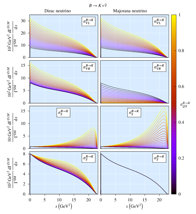
Figure 6: Comparison of various generic NP contributions in $B\to K\,\nu_{\ell}\,\overline{\nu}_{\ell}$ decay. We use the scalar and tensor NP parameters $\varepsilon_{S}$ and $\varepsilon_{T}$ as defined in Eq. (45). $\Gamma_{\textrm{SM}}$ denotes the partial decay rate of $B\to K\,\nu_{\ell}\,\overline{\nu}_{\ell}$ in the SM. Also note the different overall normalisation factors used to show the distributions more clearly.

The discussion in section 5.1 is applicable to all $\mathcal{P}_{i}\to\mathcal{P}_{f}\,\nu_{\ell}\,\overline{\nu}_{\ell}$ decays but under the set of strong assumptions which may not be satisfied in real processes. In particular, the form factor $F_{\textrm{SM}}$ is known to be in general $s$-dependent, as shown by the QCD lattice calculations. To study the effect of $s$ dependence of $F_{\textrm{SM}}$ on the distinguishing features of Dirac and Majorana neutrinos, let us analyse as an example the decay $B\to K\nu\overline{\nu}$, relaxing the assumptions we had made in Sec. 5.1. In particular, we use here the functional form of $B\to K$ form factors in the SM as given in Ref. Bouchard:2013eph and consider the full form of Eqs. (38a) and (38b) (although we have continued to assume the unknown NP form factors $\varepsilon_{X}^{B\to K}$ to be independent of $s$ for simplicity).

Without the simplifying assumptions of section 5.1, the detailed shape of $s$ distributions changes as shown in Fig. 6, but they remain visibly different for Dirac and Majorana neutrino possibilities. We note the following salient features noticeable in Fig. 6.

1. The general trends noted before in context of Fig. 5 are also clearly seen in Fig. 6. The presence of NP contributions, except the left-handed vector NP contribution, do indeed lead to different and distinguishable distributions for Dirac and Majorana neutrinos.

2. The distributions in Fig. 6 are significantly altered comparing to the ones shown in Fig. 5 for larger values of $s$, in concordance with the enhancement of $F_{\mathrm{\textrm{SM}}}$ with increasing $s$.

3. We note also that if $m_{\nu}$ is not neglected, the distributions plotted in Fig. 6 actually drop to zero at the minimal value of $s=4\,m_{\nu}^{2}$ (when the factor $b$ in the numerator of Eq. (39) vanishes). However, as $m_{\nu}$ is extremely tiny in comparison with other masses, such drop of distributions is very steep and so close to $s=0$ that it is unlikely to be observed experimentally.

We would like to also emphasise the fact that in Figs. 5 and 6, the NP parameters are shown to be positive just for the purpose of illustration. In Eqs. (38) and (48), it is clear that the scalar and tensor NP contributions are insensitive to the sign of the NP parameter. For left-handed vector NP contribution alone, both Dirac and Majorana cases yield identical $s$ distributions, where as for right-handed vector NP contribution alone, the Dirac and Majorana cases would still have opposite behaviour. Therefore, our conclusions regarding distinguishability of Dirac and Majorana nature from observed $s$ distribution still holds true, in general, even for negative NP parameters.

Study of the energy spectra of the decays with neutrino antineutrino pair in the final state is very challenging as such decays have very low branching ratios. Notably also the example considered in this section, $B\to K\nu\overline{\nu}$, has yet to be observed, although current experimental bound for it is already less than order of magnitude worse than the prediction of its SM decay rate Blake:2016olu ; Belle-II:2021rof .

In order to estimate the accuracy of spectra measurement required to see the difference between the Dirac and Majorana neutrinos, let us define the quantity

$$\Delta X=\frac{\left|X^{D}-X^{M}\right|}{X^{D}}.$$ (49)

One can assume two scenarios. First, one can estimate that the maximal size of neutrino NP couplings to be of the order of limit given in Eq. (43), so ${\cal O}(0.1)$. The second scenario assume that there is a fine tuning between NP couplings and they may be large, ${\cal O}(1)$, as shown in Fig. 4. This is possible only for $\varepsilon_{VL}$ and $\varepsilon_{VR}$ as scalar and tensor contributions to total decay branching ratios are always positive and cannot cancel out with other terms. It turns out that the relative modification of spectrum shape, given by $\Delta X$, is of the similar order as the size of the (dimensionless) coupling $\varepsilon_{X}$ themselves. This can be e.g. seen assuming that only $\varepsilon_{VR}$ does not vanish. Then one has for every $\tilde{s}$ the fixed ratio

$$\Delta X=\frac{2\left|\varepsilon_{VR}\right|}{1+\varepsilon_{VR}^{2}}.$$ (50)

Given the rarity of considered decays and statistics necessary to obtain its energy spectrum, the first scenario $\varepsilon_{VR}\sim\Delta X\sim{\cal O}(0.1)$ is unlikely to be observed at least in the near future. However, in an (optimistic!) scenario of fine tuned large NP couplings, $\varepsilon_{VR}\sim\Delta X\sim{\cal O}(1)$, the nature of neutrinos can become clear if only the decay spectrum is at all measurable, even with small accuracy. If it happens, it also points out to the type of the neutrino NP interactions, as only the right-handed vector $\varepsilon_{VR}$ couplings can simultaneously be large and lead to difference between the Dirac and Majorana case.

One should also note that Figs. 5 and 6 were plotted by taking individual non-vanishing NP neutrino couplings one at a time. In general, the real shape of spectrum can depend on several parameters and differ from those displayed in Figs. 5 and 6. In any specific NP model the effective shape is calculable and if experiment is able to measure it, fitting procedures can give the information on model parameters. However, as usual just discovery of discrepancy with the SM predictions does not immediately disclose what kind of NP interactions may be involved and further studies with combining more observables are necessary.

As the experimental accuracy of these $s$ distributions gets improved, one could be optimistic that in future with enough of detected events, such a study might become feasible. We hope that the possibility of discovering NP as well as distinguishing the Dirac and Majorana nature of neutrinos based on their different NP behaviours, would lend support to any proposal for further experimental exploration of such rare decays as $B\to K\,\nu\,\overline{\nu}$ and $K\to\pi\,\nu\,\overline{\nu}$.

6 Conclusions

In this paper, we have provided a general framework for analysing the processes containing a neutrino antineutrino pair in the final state, considering neutrinos to be either Dirac or Majorana fermions. We emphasise the fact that the quantum mechanically identical nature of Majorana neutrino and antineutrino does not depend on the size of their mass. Thus, the different statistical properties of the Dirac and Majorana neutrinos can lead, at least in the New Physics models with non-standard neutrino couplings, to significantly different predictions for the decay rates and for the spectra of visible particles. Such differences are (at least in principle) not proportional to the tiny neutrino masses, unlike the huge suppression inherently present in the neutrino-mediated Lepton Number Violating processes.

We argue that within the SM due to the particular structure of the neutrino vector-like left-handed only couplings, such not-suppressed effects of different statistics unfortunately still disappear when integrating over the phase space of final state neutrinos (excluding eventually some special kinematic scenarios where the neutrino momenta can be reconstructed or inferred, see Ref. Kim:2021dyj for more details). However, we point out that, when New Physics effects are taken into consideration, the difference between Dirac and Majorana neutrino possibilities could survive even if one neglects neutrino mass dependent terms and integrates over the phase space of final state neutrinos.

We explicitly illustrate the general analysis by examples of neutral current processes with the 2-body or 3-body final states. Using our example processes $Z\to\nu\,\overline{\nu}$ and $\mathcal{P}_{i}\to\mathcal{P}_{f}\,\nu\,\overline{\nu}$ decays, we show how the experimental bounds on the NP couplings differ between Dirac neutrino and Majorana neutrino possibilities. We also point out that if the NP terms are substantial comparing to SM couplings and the differential decay rate or equivalently the missing mass-square distribution for $\mathcal{P}_{i}\to\mathcal{P}_{f}\,\nu\,\overline{\nu}$ decay can be measured accurately enough, the shape of the spectrum can directly help discern whether neutrinos are Dirac or Majorana fermions, at least in NP models were there are no new light exotic states which could also escape detection.

References

- (1) Y. Fukuda et al. [Super-Kamiokande], “Evidence for oscillation of atmospheric neutrinos, ” Phys. Rev. Lett. 81, 1562-1567 (1998) doi:10.1103/PhysRevLett.81.1562 [arXiv:hep-ex/9807003 [hep-ex]].
- (2) Q. R. Ahmad et al. [SNO], “Direct evidence for neutrino flavor transformation from neutral current interactions in the Sudbury Neutrino Observatory, ” Phys. Rev. Lett. 89, 011301 (2002) doi:10.1103/PhysRevLett.89.011301 [arXiv:nucl-ex/0204008 [nucl-ex]].
- (3) Z. Maki, M. Nakagawa and S. Sakata, “Remarks on the unified model of elementary particles, ” Prog. Theor. Phys. 28, 870-880 (1962) doi:10.1143/PTP.28.870
- (4) B. Pontecorvo, “Neutrino Experiments and the Problem of Conservation of Leptonic Charge, ” Zh. Eksp. Teor. Fiz. 53, 1717-1725 (1967) [Sov. Phys. JETP 26 984-988 (1968)] http://www.jetp.ras.ru/cgi-bin/e/index/e/26/5/p984?a=list
- (5) P. A. Zyla et al. [Particle Data Group], “Review of Particle Physics, ” PTEP 2020, no.8, 083C01 (2020) and 2021 update. doi:10.1093/ptep/ptaa104
- (6) A. de Gouvêa, “Neutrino Mass Models, ” Ann. Rev. Nucl. Part. Sci. 66, 197-217 (2016) doi:10.1146/annurev-nucl-102115-044600
- (7) Y. Cai, J. Herrero-García, M. A. Schmidt, A. Vicente and R. R. Volkas, “From the trees to the forest: a review of radiative neutrino mass models, ” Front. in Phys. 5, 63 (2017) doi:10.3389/fphy.2017.00063 [arXiv:1706.08524 [hep-ph]].
- (8) E. Majorana, “Teoria simmetrica dell’elettrone e del positrone, ” Nuovo Cim. 14, 171-184 (1937) doi:10.1007/BF02961314
- (9) G. Racah, “On the symmetry of particle and antiparticle, ” Nuovo Cim. 14, 322-328 (1937) doi:10.1007/BF02961321
- (10) W. H. Furry, “Note on the Theory of the Neutral Particle, ” Phys. Rev. 54, 56-67 (1938) doi:10.1103/PhysRev.54.56
- (11) F. T. Avignone, III, S. R. Elliott and J. Engel, “Double Beta Decay, Majorana Neutrinos, and Neutrino Mass, ” Rev. Mod. Phys. 80, 481-516 (2008) doi:10.1103/RevModPhys.80.481 [arXiv:0708.1033 [nucl-ex]].
- (12) K. Blaum, S. Eliseev, F. A. Danevich, V. I. Tretyak, S. Kovalenko, M. I. Krivoruchenko, Y. N. Novikov and J. Suhonen, “Neutrinoless Double-Electron Capture, ” Rev. Mod. Phys. 92, 045007 (2020) doi:10.1103/RevModPhys.92.045007 [arXiv:2007.14908 [hep-ph]].
- (13) M. Lee and M. MacKenzie, “Muon to Positron Conversion,” Universe 8, no.4, 227 (2022) doi:10.3390/universe8040227 [arXiv:2110.07093 [hep-ex]].
- (14) J. A. Grifols, E. Masso and R. Toldra, “Majorana neutrinos and long range forces, ” Phys. Lett. B 389, 563-565 (1996) doi:10.1016/S0370-2693(96)01304-4 [arXiv:hep-ph/9606377 [hep-ph]].
- (15) F. Ferrer, J. A. Grifols and M. Nowakowski, “Long range forces induced by neutrinos at finite temperature, ” Phys. Lett. B 446, 111-116 (1999) doi:10.1016/S0370-2693(98)01489-0 [arXiv:hep-ph/9806438 [hep-ph]].
- (16) A. Segarra and J. Bernabéu, “Absolute neutrino mass and the Dirac/Majorana distinction from the weak interaction of aggregate matter, ” Phys. Rev. D 101, no.9, 093004 (2020) doi:10.1103/PhysRevD.101.093004 [arXiv:2001.05900 [hep-ph]].
- (17) A. Costantino and S. Fichet, “The Neutrino Casimir Force, ” JHEP 09, 122 (2020) doi:10.1007/JHEP09(2020)122 [arXiv:2003.11032 [hep-ph]].
- (18) M. Ghosh, Y. Grossman and W. Tangarife, “Probing the two-neutrino exchange force using atomic parity violation, ” Phys. Rev. D 101, no.11, 116006 (2020) doi:10.1103/PhysRevD.101.116006 [arXiv:1912.09444 [hep-ph]].
- (19) P. D. Bolton, F. F. Deppisch and C. Hati, “Probing new physics with long-range neutrino interactions: an effective field theory approach, ” JHEP 07, 013 (2020) doi:10.1007/JHEP07(2020)013 [arXiv:2004.08328 [hep-ph]].
- (20) X. j. Xu and B. Yu, “On the short-range behavior of neutrino forces beyond the Standard Model: from 1/r5 to 1/r4, 1/r2, and 1/r, ” JHEP 02, 008 (2022) doi:10.1007/JHEP02(2022)008 [arXiv:2112.03060 [hep-ph]].
- (21) M. Ghosh, Y. Grossman, W. Tangarife, X. J. Xu and B. Yu, “Neutrino forces in neutrino backgrounds,” [arXiv:2209.07082 [hep-ph]].
- (22) G. Cvetic, C. Dib, S. K. Kang and C. S. Kim, “Probing Majorana neutrinos in rare and meson decays,” Phys. Rev. D 82, 053010 (2010) doi:10.1103/PhysRevD.82.053010 [arXiv:1005.4282 [hep-ph]].
- (23) D. Q. Adams et al. [CUORE], “Search for Majorana neutrinos exploiting millikelvin cryogenics with CUORE,” Nature 604, no.7904, 53-58 (2022) doi:10.1038/s41586-022-04497-4 [arXiv:2104.06906 [nucl-ex]].
- (24) B. Kayser and R. E. Shrock, “Distinguishing Between Dirac and Majorana Neutrinos in Neutral Current Reactions, ” Phys. Lett. B 112, 137-142 (1982) doi:10.1016/0370-2693(82)90314-8
- (25) S. P. Rosen, “Analog of the Michel Parameter for Neutrino - Electron Scattering: A Test for Majorana Neutrinos, ” Phys. Rev. Lett. 48, 842 (1982) doi:10.1103/PhysRevLett.48.842
- (26) G. V. Dass, “Distinguishing between Dirac and Majorana neutrinos in neutrino-electron scattering,” Phys. Rev. D 32, 1239 (1985) doi:10.1103/PhysRevD.32.1239
- (27) W. Rodejohann, X. J. Xu and C. E. Yaguna, “Distinguishing between Dirac and Majorana neutrinos in the presence of general interactions,” JHEP 05, 024 (2017) doi:10.1007/JHEP05(2017)024 [arXiv:1702.05721 [hep-ph]].
- (28) A. Millar, G. Raffelt, L. Stodolsky and E. Vitagliano, “Neutrino mass from bremsstrahlung endpoint in coherent scattering on nuclei,” Phys. Rev. D 98, no.12, 123006 (2018) doi:10.1103/PhysRevD.98.123006 [arXiv:1810.06584 [hep-ph]].
- (29) B. Kayser, “Majorana Neutrinos and their Electromagnetic Properties, ” Phys. Rev. D 26, 1662 (1982) doi:10.1103/PhysRevD.26.1662
- (30) J. Schechter and J. W. F. Valle, “Majorana Neutrinos and Magnetic Fields,” Phys. Rev. D 24, 1883-1889 (1981) [erratum: Phys. Rev. D 25, 283 (1982)] doi:10.1103/PhysRevD.25.283
- (31) R. E. Shrock, “Implications of Neutrino Masses and Mixing for the Mass, Width, and Decays of the ,” eConf C8206282, 261-263 (1982) ITP-SB-82-52.
- (32) E. Ma and J. T. Pantaleone, “Heavy-Majorana-neutrino production,” Phys. Rev. D 40, 2172-2176 (1989) doi:10.1103/PhysRevD.40.2172
- (33) J. F. Nieves and P. B. Pal, “Majorana neutrinos and photinos from kaon decay,” Phys. Rev. D 32, 1849-1852 (1985) doi:10.1103/PhysRevD.32.1849
- (34) T. Chhabra and P. R. Babu, “Way to distinguish between Majorana and Dirac massive neutrinos in neutrino counting reactions,” Phys. Rev. D 46, 903-909 (1992) doi:10.1103/PhysRevD.46.903
- (35) J. M. Berryman, A. de Gouvêa, K. J. Kelly and M. Schmitt, “Shining light on the mass scale and nature of neutrinos with ,” Phys. Rev. D 98, no.1, 016009 (2018) doi:10.1103/PhysRevD.98.016009 [arXiv:1805.10294 [hep-ph]].
- (36) M. Yoshimura and N. Sasao, “Radiative emission of neutrino pair from nucleus and inner core electrons in heavy atoms,” Phys. Rev. D 89, no.5, 053013 (2014) doi:10.1103/PhysRevD.89.053013 [arXiv:1310.6472 [hep-ph]].
- (37) C. S. Kim, M. V. N. Murthy and D. Sahoo, “Inferring the nature of active neutrinos: Dirac or Majorana?,” Phys. Rev. D 105, no.11, 113006 (2022) doi:10.1103/PhysRevD.105.113006 [arXiv:2106.11785 [hep-ph]].
- (38) E. Goudzovski, D. Redigolo, K. Tobioka, J. Zupan, G. Alonso-Álvarez, D. S. M. Alves, S. Bansal, M. Bauer, J. Brod and V. Chobanova, et al. “New Physics Searches at Kaon and Hyperon Factories,” doi:10.1088/1361-6633/ac9cee [arXiv:2201.07805 [hep-ph]].
- (39) A. Denner, H. Eck, O. Hahn and J. Kublbeck, “Feynman rules for fermion number violating interactions,” Nucl. Phys. B 387, 467-481 (1992) doi:10.1016/0550-3213(92)90169-C
- (40) J. M. Márquez, G. L. Castro and P. Roig, “Michel parameters in the presence of massive Dirac and Majorana neutrinos,” [arXiv:2208.01715 [hep-ph]].
- (41) P. Janot and S. Jadach, “Improved Bhabha cross section at LEP and the number of light neutrino species,” Phys. Lett. B 803, 135319 (2020) doi:10.1016/j.physletb.2020.135319 [arXiv:1912.02067 [hep-ph]].
- (42) E. Cortina Gil et al. [NA62], “Measurement of the very rare decay,” JHEP 06, 093 (2021) doi:10.1007/JHEP06(2021)093 [arXiv:2103.15389 [hep-ex]].
- (43) A. J. Buras, D. Buttazzo, J. Girrbach-Noe and R. Knegjens, “ and in the Standard Model: status and perspectives,” JHEP 11, 033 (2015) doi:10.1007/JHEP11(2015)033 [arXiv:1503.02693 [hep-ph]].
- (44) T. Blake, G. Lanfranchi and D. M. Straub, “Rare Decays as Tests of the Standard Model,” Prog. Part. Nucl. Phys. 92, 50-91 (2017) doi:10.1016/j.ppnp.2016.10.001 [arXiv:1606.00916 [hep-ph]].
- (45) F. Abudinén et al. [Belle-II], “Search for Decays Using an Inclusive Tagging Method at Belle II,” Phys. Rev. Lett. 127, no.18, 181802 (2021) doi:10.1103/PhysRevLett.127.181802 [arXiv:2104.12624 [hep-ex]].
- (46) C. S. Kim, S. C. Park and D. Sahoo, “Angular distribution as an effective probe of new physics in semihadronic three-body meson decays,” Phys. Rev. D 100, no.1, 015005 (2019) doi:10.1103/PhysRevD.100.015005 [arXiv:1811.08190 [hep-ph]].
- (47) C. Bouchard et al. [HPQCD], “Rare decay form factors from lattice QCD,” Phys. Rev. D 88, no.5, 054509 (2013) [erratum: Phys. Rev. D 88, no.7, 079901 (2013)] doi:10.1103/PhysRevD.88.054509 [arXiv:1306.2384 [hep-lat]].