A bivariate functional copula joint model for longitudinal measurements and time-to-event data

Abstract

A bivariate functional copula joint model, which models the repeatedly measured longitudinal outcome at each time point with the survival data, jointly by both random effects and bivariate functional copulas, is proposed in this paper. A regular joint model normally supposes there are some subject-specific latent random effects or classes shared by the longitudinal and time-to-event processes and they are assumed to be conditionally independent given these latent random variables. Under this assumption, the joint likelihood of the two processes can be easily derived and the association between them, as well as heterogeneity among population are naturally introduced by the unobservable latent random variables. However, because of the unobservable nature of these latent variables, the conditional independence assumption is difficult to verify. Therefore, a bivariate functional copula is introduced into a regular joint model to account for the cases where there could be extra association between the two processes which cannot be captured by the latent random variables. Our proposed model includes a regular joint model as a special case when the correlation function, which is modelled continuously by B-spline basis functions as a function of time $t,$ is constant at 0 under the bivariate Gaussian copula. Simulation studies and dynamic prediction of survival probabilities are conducted to compare the performance of the proposed model with the regular joint model and a real data application on the Primary biliary cirrhosis (PBC) data is performed.

1 Introduction

Joint modelling of longitudinal measurements and time-to-event data has become increasingly popular in recent decades, as previous studies indicate separately modelling (Tsiatis et al., 1995[40] and Guo and Carlin, 2004[13]) or a two-stage modelling (Wulfsohn and Tsiatis, 1997[42]) of the two processes can result in biased estimations due to not fully considering the association between the two sub-models. The classical joint model in Faucett and Thomas, (1996)[9] and Wulfsohn and Tsiatis (1997)[42] assumes a linear mixed effects model and a proportional hazard model for the longitudinal and survival sub-models, respectively. Thereafter, joint models with non-linear mixed longitudinal process modelled by cubic B-splines or functional principal components have been by proposed Brown et al. (2005)[4], Yao (2007)[43] and Li et al. (2021)[20]. Li and Luo (2017)[21] and (2019)[22] incorporate functional covariates, which is a continuous curve over some domain, into the joint model. A latent class joint model is discussed by Lin et al. (2002)[24], (2004)[23] and Proust-Lima et al. (2009)[29]. Excellent overviews on joint modelling can be found in Tsiatis and Davidian (2004)[39], Ibrahim et al. (2010)[17], Papageorgiou et al. (2019)[28] and Alsefri et al. (2020)[1]. Despite the diverse extension of the joint modelling framework in recent years, conditional independence of the two sub-models given the latent variables is an assumption which has always remained stable. This assumption is tricky to verify as the latent variables are not observable. Roy (2003)[36], Guo et al. (2006)[12] and Jacqmin-Gadda et al. (2010)[19] proposed some tests to assess conditional independence given latent classes via a score test or testing the dependency within each class after randomly allocating the subjects into classes using the estimated posterior class-membership probabilities, but these tests apply only to the latent class joint model.

Emura et al., (2017)[8] pointed out joint analysis of two survival outcomes, such as death and relapse of cancer, by a joint frailty model (Rondeau et al., 2015[35]), where conditional independence between the two survival outcomes is assumed, given a shared study-specific frailty term, may not be sufficient to account for all the dependency between outcomes in a subject level, especially when the covariates information are insufficiently collected. For this reason, they introduced a joint frailty-copula model, which associates the two survival outcomes by both shared frailty terms and copula. It is reasonable to have the same doubts about conditional independence in the joint modelling of longitudinal and time-to-event data when there are only a few covariates or the latent variable structure is too simple. To alleviate this issue, Henderson et al. (2000)[14] replaced the simple shared random effects in the two sub-models by a combination of correlated random effects and a mean-zero bivariate Gaussian stochastic process, representing a long-term trend and local variation at subject-level. However, the infinite dimension of the stochastic process comes with intensive computation and the baseline hazard function is only allowed to be modelled nonparametrically by taking mass at each failure time due to integrability issues. In addition, Hsieh et al. (2006)[16] pointed out the unspecified baseline hazard leads to underestimation of the standard errors for parameters in the EM algorithm. Similar to Henderson et al. (2000)[14], Wang et al. (2001)[41] applied a random intercept and an integrated Ornstein-Uhlenbeck stochastic process for the latent variables. As a compromise, the stochastic process was treated as a piecewise constant function for estimation. In more recent work, Dutta et al. (2021)[7] modelled the joint distribution of log-transformed survival time and the longitudinal measurement, conditional on shared random effects by a multivariate normal distribution. This model introduced dependency between the two processes by both random effects and the covariance matrix of the multivariate normal distribution but the assumption on the event time distribution may be too restrictive.

Associating the longitudinal and survival sub-models by copula (Hofert et al., 2018)[15] has also been considered recently. Rizopoulos et al. (2008a[33], 2008b[34]) and Malehi et al. (2015)[25] applied copulas to model the joint distribution of the latent random effects, which offered greater flexibility of association compared with the traditional shared random effects joint model, by allowing different copulas and marginals distributions. However, conditional independence is still assumed in these models. Applying multivariate copulas directly on marginals of all the longitudinal measurements and event time data for each subject was considered by Ganjali and Baghfalaki (2015)[10] and Zhang et al.(2021a)[44]. The non-linear correlation introduced by the copula between the two sub-models is different to the linear correlation arising from latent random effects, but the lack of random effects in the joint models compromises their capability to capture the longitudinal trajectories at the subject level. Besides, the difficulty of modelling the correlation matrix in the copula increases with the number of longitudinal measurements. Zhang et al.(2021b)[45] further proposed modelling the joint distribution of all the longitudinal and survival outcomes in each subject, given random effects, by multivariate Gaussian copula. This model has two layers of correlation between the two sub-models and a regular joint model of conditional independence becomes a specially case when the correlation matrix in the multivariate Gaussian copula is an identity matrix. However, the modelling of the correlation matrix is still problematic, especially when the correlation matrix is large. The approach of Suresh et al.(2021a)[37] and (2021b)[38] can solve this issue by applying bivariate Gaussian copulas on the conditional joint distribution of survival time and a longitudinal measurement at a single time point given the subject being alive by that time point, since the correlation matrix of a two-dimensional copula is easier to model. But their model still falls under the marginal models as Ganjali and Baghfalaki (2015)[10] and Zhang et al.(2021a)[44] since it does not have latent effects.

In this paper, we propose a functional bivariate copula joint model by modelling the conditional joint distribution of survival time and a single longitudinal measurement, conditional on random effects and that the subject survives beyond the time point of this longitudinal measurement, through a bivariate functional copula. The correlation function in this bivariate copula is modelled by B-splines. The remainder of the paper is organised as followed. Section 2 describes the notations and specification of the proposed model. In Section 3, simulations are conducted to assess the performance of the proposed model in terms of parameter estimation and dynamic prediction of survival probabilities by comparing with a regular joint model which assumes conditional independence. A real data application is carried out in Section 4. The limitations of the proposed model are discussed and some future work is suggested in Section 5.

2 Functional bivariate copula joint model framework

In a clinical study, suppose there are $n$ subjects being followed over a period of time. For the $i$th, $i=1,...,n,$ subject, its longitudinal observations $\bm{y}_{i}=\left\{y_{i1}=y_{i}(s_{i1}),...,y_{in_{i}}=y_{i}(s_{in_{i}})\right\}^{{}^{\prime}}$ are measured intermittently at time points $\bm{s}_{i}=(s_{i1},...,s_{in_{i}})$ and are terminated by the observed event time $T_{i}=\mbox{min}(C_{i},T_{i}^{*})$ with $C_{i}$ and $T_{i}^{*}$ being the right censoring time and true event time, respectively. Thus, observing a longitudinal measurement $y_{ij}$ at $s_{ij},$ $1\leq j\leq n_{i},$ implicitly implies $y_{ij}|T_{i}^{*}>s_{ij}.$ We also denote $\delta_{i}=I(T_{i}^{*}<C_{i})$ as the corresponding event indicator, which takes value 1 if the true event time is observed and 0 otherwise, for subject $i.$ The observation time points $\bm{s}_{i}$ and the censoring process $C_{i}$ are assumed to be uninformative conditional on the baseline covariates.

Suppose the longitudinal process for subject $i$ is specified by the following model:

$$y_{ij}=\bm{x}_{ij}^{{}^{\prime}}\bm{\beta}_{1}+\bm{z}_{ij}^{{}^{\prime}}\bm{b}_{i}+\varepsilon_{ij},\mbox{ }i=1,...,n,\mbox{ }j=1,...,n_{i},$$ (1)

where $\bm{x}_{ij}=x_{i}(s_{ij})$ is a $p\times 1$ baseline covariate vector with fixed effects $\bm{\beta}_{1},$ $\bm{z}_{ij}=z_{i}(s_{ij})$ is a $r\times 1$ covariate vector for random effects $\bm{b}_{i}\sim N_{r}(\bm{0},\bm{D}),$ and the error term $\displaystyle\varepsilon_{ij}=\varepsilon_{i}(s_{ij})\sim N(0,\sigma^{2}).$

The corresponding survival process for this subject is given by a proportional hazard model (Cox, 1972[5]) with frailty terms as:

$$h_{i}(t)=h_{0}(t)\mbox{exp}(\bm{w}_{i}^{{}^{\prime}}\bm{\beta}_{2}+\bm{z}_{i}(t)^{{}^{\prime}}(\bm{\alpha}\circ\bm{b}_{i})),$$ (2)

where $\bm{w}_{i}$ is a $q\times 1$ vector of baseline explanatory variables for the survival process with associated regression parameter vector $\bm{\beta}_{2},$ the $r$-dimensional vector $\bm{\alpha}$ characterises the dependency between the two sub-models and $\circ$ is the Hadamard product. Common covariates are allowed for $\bm{x}_{i}$ and $\bm{w}_{i}$. The baseline hazard function is common for all subjects and assumed to be a piecewise-constant function having $K-1$ equally spaced internal knots as:

$$h_{0}(t)=\sum_{k=1}^{K}\lambda_{k}I(v_{k-1}<t\leq v_{k}),$$

where $0=v_{0}<v_{1}<\cdots<v_{K}=t_{max}=\mbox{max}\left\{t_{i},\mbox{ }i=1,...,n\right\},$ such that $[0,t_{max}]$ is split into $K$ intervals, each with a constant baseline hazard $\lambda_{k}$.

According to the recording time point $\bm{s}_{i}$ of the longitudinal process, the information contributed by subject $i$ can be described in a progressive way as follows:

1. At the origin of the two processes, i.e. at $t=0,$ some baseline covariates are taken. Does the event occur before the first scheduled longitudinal measurement planned at $t=s_{i1}?$ If not, the two processes continue;

2. At $t=s_{ij},$ $j=1,...,n_{i}-1,$ a longitudinal measurement is observed and we monitor if the event is censored or observed before the next scheduled longitudinal measurement planned at $t=s_{i(j+1)}.$ If not, the two processes continue;

3. At $t=s_{in_{i}},$ a longitudinal measurement is observed, then the event is censored or observed at $t=t_{i}$ before the next longitudinal measurement can be recorded. The two processes are terminated at $t=t_{i}$ with an associated event indicator $\delta_{i}.$

The above steps decompose the observed likelihood of subject $i$ as:

$$L_{i} = f_{T_{i}^{*},\bm{y}_{i}}(t_{i},\bm{y}_{i})$$ (3)

$$= f_{T_{i}^{*}}(T_{i}^{*}>s_{i1})\times f_{T_{i}^{*},y_{i1}}(T_{i}^{*}>s_{i2},y_{i1}|T_{i}^{*}>s_{i1})\times f_{T_{i}^{*},y_{i2}}(T_{i}^{*}>s_{i3},y_{i2}|T_{i}^{*}>s_{i2},y_{i1})\times\cdots$$

$$\times f_{T_{i}^{*},y_{i(n_{i}-1)}}(T_{i}^{*}>s_{in_{i}},y_{i(n_{i}-1)}|T_{i}^{*}>s_{i(n_{i}-1)},y_{i1},...,y_{i(n_{i}-2)})$$

$$\times f_{T_{i}^{*},y_{in_{i}}}(T_{i}^{*}>t_{i},y_{in_{i}}|T_{i}^{*}>s_{in_{i}},y_{i1},...,y_{i(n_{i}-1)})^{1-\delta_{i}}$$

$$\times f_{T_{i}^{*},y_{in_{i}}}(T_{i}^{*}=t_{i},y_{in_{i}}|T_{i}^{*}>s_{in_{i}},y_{i1},...,y_{i(n_{i}-1)})^{\delta_{i}}.$$

If the first longitudinal measurement is taken at the origin, i.e., $s_{i1}=0,$ the first two terms in (3) can be merged as $f_{T_{i}^{*},y_{i1}}(T_{i}^{*}>s_{i2},y_{i1}).$ Each term can be interpreted as the information updated between interval $[s_{ij},s_{i(j+1)})$ conditional on the previous information. Suppose the dependency between the information in each interval are introduced by the subject-specific random effects $\bm{b}_{i},$ then we can rewrite (3) as:

$$L_{i}(\bm{\theta}) = f_{T_{i}^{*},\bm{y}_{i}}(t_{i},\bm{y}_{i})$$ (4)

$$= \int_{\bm{b}_{i}}f_{T_{i}^{*}}(T_{i}^{*}>s_{i1}|\bm{b}_{i})\times f_{T_{i}^{*},y_{i1}}(T_{i}^{*}>s_{i2},y_{i1}|T_{i}^{*}>s_{i1},\bm{b}_{i})\times f_{T_{i}^{*},y_{i2}}(T_{i}^{*}>s_{i3},y_{i2}|T_{i}^{*}>s_{i2},\bm{b}_{i})\times\cdots$$

$$\times f_{T_{i}^{*},y_{i(n_{i}-1)}}(T_{i}^{*}>s_{in_{i}},y_{i(n_{i}-1)}|T_{i}^{*}>s_{i(n_{i}-1)},\bm{b}_{i})$$

$$\times f_{T_{i}^{*},y_{in_{i}}}(T_{i}^{*}>t_{i},y_{in_{i}}|T_{i}^{*}>s_{in_{i}},\bm{b}_{i})^{1-\delta_{i}}$$

$$\times f_{T_{i}^{*},y_{in_{i}}}(T_{i}^{*}=t_{i},y_{in_{i}}|T_{i}^{*}>s_{in_{i}},\bm{b}_{i})^{\delta_{i}}\,d\bm{b}_{i}.$$

According to the specification of the two sub-models in (1) and (2), the distribution of the two sub-models conditional on random effects $\bm{b}_{i}$ and subject $i$ has survived up to $t=s_{ij}$ are given by:

$$F_{T_{i}^{*}}(t|\bm{b}_{i},T_{i}^{*}>s_{ij})=1-\mbox{exp}\left(-\int_{s_{ij}}^{t}h_{i}(u)du\right),$$

and

$$F_{y_{ij}}(y_{ij}|\bm{b}_{i},T_{i}^{*}>s_{ij})=\Phi\left(\frac{y_{ij}-\bm{x}_{i}^{{}^{\prime}}\bm{\beta}_{1}-\bm{z}_{ij}^{{}^{\prime}}\bm{b}_{i}}{\sigma}\right).$$

In the remaining paper, we denote $\displaystyle U_{t|\bm{b}_{i},s_{ij}}=F_{T_{i}^{*}}(t|\bm{b}_{i},T_{i}^{*}>s_{ij})$ and $\displaystyle U_{y_{ij}|\bm{b}_{i},s_{ij}}=F_{y_{ij}}(y_{ij}|\bm{b}_{i},T_{i}^{*}>s_{ij})$ for convenience. The joint distribution of $U_{t|\bm{b}_{i},s_{ij}}$ and $U_{y_{ij}|\bm{b}_{i},s_{ij}}$ at each $s_{ij}$ is modelled by bivariate copulas with their Kendall’s correlation being a function of time. The bivariate Gaussian and $t$ copulas are considered here since their Kendall’s tau can range from -1 to 1 while other copulas, such as bivariate Archimedean copulas, do not have this nice property. In addition, under these two copulas, Kendall’s $\tau(t)$ is simply a function of Pearson’s correlation as $\displaystyle\tau(t)=\frac{2}{\pi}\mbox{arcsin}\rho(t).$ This nice property allows us to model Kendall’s $\tau(t)$ between $T_{i}$ and $y_{i}(t)$ continuously through modelling $\rho(t)$, which is easier under the bivariate Gaussian and $t$ copulas. Let $\phi(\cdot),$ $\Phi(\cdot)$ and $\psi(\cdot;\nu),$ $\Psi(\cdot;\nu)$ be the pdfs and cdfs of the standard normal distribution and Student’s $t$ distribution with $\nu$ degrees of freedom, respectively.

2.1 Functional bivariate Gaussian copula joint model

Suppose the bivariate Gaussian copula is applied to characterise the joint distribution of $\displaystyle U_{t|\bm{b}_{i},s_{ij}}$ and $\displaystyle U_{y_{ij}|\bm{b}_{i},s_{ij}}.$ Let $\displaystyle Z_{t|\bm{b}_{i},s_{ij}}=\Phi^{-1}\left(U_{t|\bm{b}_{i},s_{ij}}\right)$ and $\displaystyle Z_{y_{ij}|\bm{b}_{i},s_{ij}}=\Phi^{-1}\left(U_{y_{ij}|\bm{b}_{i},s_{ij}}\right)=\frac{y_{ij}-\bm{x}_{ij}^{{}^{\prime}}\bm{\beta}_{1}-\bm{z}_{ij}^{{}^{\prime}}\bm{b}_{i}}{\sigma}.$ The Pearson’s correlation $\rho(s_{ij})$ between $\displaystyle Z_{t|\bm{b}_{i},s_{ij}}$ and $\displaystyle Z_{y_{ij}|\bm{b}_{i},s_{ij}}$ is treated as a smooth function of time.

Let $\bm{\phi}_{2}(\cdot;\sigma)$ denote the pdf of a bivariate standardised normal random vector with mean $\bm{0}$ and correlation $\rho$. The likelihood contributed by $T_{i}^{*}>t,y_{ij}|T_{i}^{*}>\tau_{ij},\bm{b}_{i},$ $j=1,...,n_{i},$ is given by:

$$\displaystyle f_{T_{i}^{*},y_{ij}}(T_{i}^{*}>t,y_{ij}|\bm{b}_{i},T_{i}^{*}>s_{ij})=\sigma^{-1}\Phi\left(-\frac{Z_{t|\bm{b}_{i},s_{ij}}-\rho(s_{ij})Z_{y_{ij}|\bm{b}_{i},s_{ij}}}{\sqrt{1-\rho(s_{ij})^{2}}}\right)\phi\left(Z_{y_{ij}|\bm{b}_{i},s_{ij}}\right),$$ (5)

while the likelihood contributed by $T_{i}^{*}=t,y_{in_{i}}|T_{i}^{*}>s_{in_{i}},\bm{b}_{i}$ is given by:

$$\displaystyle f_{T_{i}^{*},y_{in_{i}}}(T_{i}^{*}=t,y_{in_{i}}|\bm{b}_{i},T_{i}^{*}>s_{in_{i}})=\sigma^{-1}\bm{\phi}_{2}\left(Z_{t|\bm{b}_{i},s_{in_{i}}},Z_{y_{in_{i}}|\bm{b}_{i},s_{in_{i}}};\rho(s_{in_{i}})\right)\frac{f_{T_{i}^{*}}(t|\bm{b}_{i},T_{i}^{*}>s_{in_{i}})}{\phi\left(Z_{t|\bm{b}_{i},s_{in_{i}}}\right)},$$ (6)

The observed likelihood under the functional bivariate Gaussian copula joint model can be obtained by substituting (5) and (6) back into (4).

2.2 Functional bivariate $t$ copula joint model

Suppose the bivariate $t$ copula is used to characterise the joint distribution of $\displaystyle U_{t|\bm{b}_{i},s_{ij}}$ and $\displaystyle U_{y_{ij}|\bm{b}_{i},s_{ij}}.$ Let $\displaystyle W_{t|\bm{b}_{i},s_{ij}}^{\nu}=\Psi^{-1}\left(U_{t|\bm{b}_{i},s_{ij}};\nu\right)$ and $\displaystyle W_{y_{ij}|\bm{b}_{i},s_{ij}}^{\nu}=\Psi^{-1}\left(U_{y_{ij}|\bm{b}_{i},s_{ij}};\nu\right).$ The correlation $\rho(s_{ij})$ between $\displaystyle W_{t|\bm{b}_{i},s_{ij}}^{\nu}$ and $\displaystyle W_{y_{ij}|\bm{b}_{i},s_{ij}}^{\nu}$ is treated as a smooth function of time and the variance-covariance matrix is given by:

$$\displaystyle\bm{\Sigma}(s_{ij})=\frac{\nu}{\nu-2}\bm{R}(s_{ij})=\frac{\nu}{\nu-2}\left(\begin{array}[]{ll}\displaystyle 1&\rho(s_{ij})\\ \displaystyle\rho(s_{ij})&1\end{array}\right),\mbox{ for }\nu>2.$$

Let $\bm{\psi}_{2}(\cdot;\bm{\Sigma},\nu)$ denote the pdf of a bivariate $t$ random vector with mean $\bm{0},$ scale matrix $\bm{\Sigma}$ and $\nu$ degrees of freedom. The likelihood contributed by $T_{i}^{*}>t,y_{ij}|T_{i}^{*}>s_{ij},\bm{b}_{i},$ $j=1,...,n_{i},$ is given by:

$$\displaystyle f_{T_{i}^{*},y_{ij}}(T_{i}^{*}>t,y_{ij}|\bm{b}_{i},T_{i}^{*}>s_{ij}) = \sigma^{-1}\Psi\left(-\frac{W_{t|\bm{b}_{i},s_{ij}}^{\nu}-\rho(s_{ij})W_{y_{ij}|\bm{b}_{i},s_{ij}}^{\nu}}{\sigma(s_{ij}|\bm{b}_{i},y_{ij})};\nu+1\right)$$ (8)

$$\times\phi\left(\frac{y_{ij}-\bm{x}_{ij}^{{}^{\prime}}\bm{\beta}_{1}-\bm{z}_{ij}^{{}^{\prime}}\bm{b}_{i}}{\sigma}\right),$$

while the likelihood contributed by $T_{i}^{*}=t,y_{in_{i}}|T_{i}^{*}>s_{in_{i}},\bm{b}_{i}$ is given by:

$$\displaystyle f_{T_{i}^{*},y_{in_{i}}}(T_{i}^{*}=t,y_{in_{i}}|\bm{b}_{i},T_{i}^{*}>s_{in_{i}}) = \sigma^{-1}\bm{\psi}_{2}\left(W_{t|\bm{b}_{i},s_{in_{i}}}^{\nu},W_{y_{in_{i}}|\bm{b}_{i},s_{in_{i}}}^{\nu};\bm{R}(s_{in_{i}}),\nu\right)\frac{f_{T_{i}^{*}}(t|\bm{b}_{i},T_{i}^{*}>s_{in_{i}})}{\psi\left(W_{t|\bm{b}_{i},s_{in_{i}}}^{\nu};\nu\right)}$$ (9)

$$\times\frac{\phi\left(\frac{y_{in_{i}}-\bm{x}_{in_{i}}^{{}^{\prime}}\bm{\beta}_{1}-\bm{z}_{in_{i}}^{{}^{\prime}}\bm{b}_{i}}{\sigma}\right)}{\psi\left(W_{y_{in_{i}}|\bm{b}_{i},s_{in_{i}}}^{\nu};\nu\right)},$$

where $\displaystyle\sigma(s_{ij}|\bm{b}_{i},y_{ij})^{2}=\frac{\left[\nu+(W_{y_{ij}|\bm{b}_{i},s_{ij}}^{\nu})^{2}\right]\left[1-\rho(s_{ij})^{2}\right]}{\nu+1}.$ The observed likelihood under the functional bivariate $t$ copula joint model can be obtained by substituting (9) and (8) back into (4).

2.3 Likelihood maximisation

The integrals in terms of random effects in (4) do not have a closed form expression under either the bivariate Gaussian or $t$ copula joint model, thus a multivariate Gaussian quadrature technique (Jäckel, 2005[18]) is applied to approximate the integration. However, the common weighting kernel $f_{\bm{b}_{i}}(\bm{b}_{i})$ and its quadrature points do not consider subject level information, thus they always concentrate around $\bm{0},$ while the main mass of the integrand in (4) is more likely to locate around the subject-specific random effects. The inconsistency of the quadrature points and main mass of the integrand can result in an inaccurate numerical approximation even with a large number of quadrature points. For faster and more accurate calculation, we adopt a similar approach to the adaptive Gauss-Hermite rule in Rizopoulos (2012b)[32] by rearranging (4) as:

$$f_{T_{i},\bm{y}_{i}}(t_{i},\bm{y}_{i})$$ (10)

$$= \int_{\bm{b}_{i}}f_{T_{i},\bm{y}_{i},\bm{b}_{i}}(t_{i},\bm{y}_{i},\bm{b}_{i})\,d\bm{b}_{i}$$

$$= \int_{\bm{b}_{i}}f_{\bm{y}_{i}}(\bm{y}_{i})f_{T_{i}}(t_{i}|\bm{y}_{i},\bm{b}_{i})f_{\bm{b}_{i}}(\bm{b}_{i}|\bm{y}_{i})\,d\bm{b}_{i}$$

$$= f_{\bm{y}_{i}}(\bm{y}_{i})\int_{\bm{b}_{i}}f_{T_{i}}(t_{i}|\bm{y}_{i},\bm{b}_{i})f_{\bm{b}_{i}}(\bm{b}_{i}|\bm{y}_{i})\,d\bm{b}_{i}$$

$$= \bm{\phi}_{n_{i}}\left(y_{i1}-\bm{x}_{i}^{{}^{\prime}}\bm{\beta}_{1},...,y_{in_{i}}-\bm{x}_{i}^{{}^{\prime}}\bm{\beta}_{1};\bm{V}_{\bm{y}_{i}}\right)\int_{\bm{b}_{i}}f_{T_{i}}(t_{i}|\bm{y}_{i},\bm{b}_{i})f_{\bm{b}_{i}}(\bm{b}_{i}|\bm{y}_{i})\,d\bm{b}_{i},$$

where $\displaystyle\bm{V}_{\bm{y}_{i}}=(\bm{z}_{i1}\cdots\bm{z}_{in_{i}})^{{}^{\prime}}\bm{D}(\bm{z}_{i1}\cdots\bm{z}_{in_{i}})+\sigma^{2}\bm{I}_{n_{i}},$ $f_{\bm{b}_{i}}(\bm{b}_{i}|\bm{y}_{i})$ can be derived by the joint normality of $\bm{y}_{i}$ and $\bm{b}_{i},$

$$\displaystyle f_{T_{i}}(t_{i}|\bm{y}_{i},\bm{b}_{i}) = S_{T_{i}^{*}}(s_{i1}|\bm{b}_{i})\left\{\prod_{j=1}^{n_{i}-1}\Phi\left(-\frac{Z_{s_{i(j+1)}|\bm{b}_{i},s_{ij}}-\rho(s_{ij})Z_{y_{ij}|\bm{b}_{i},s_{ij}}}{\sqrt{1-\rho(s_{ij})^{2}}}\right)\right\}^{I(n_{i}\geq 2)}$$

$$\times \left\{\frac{1}{\sqrt{1-\rho(s_{in_{i}})^{2}}}\phi\left(\frac{Z_{t_{i}|\bm{b}_{i},s_{in_{i}}}-\rho(s_{in_{i}})Z_{y_{in_{i}}|\bm{b}_{i},s_{in_{i}}}}{\sqrt{1-\rho(s_{in_{i}})^{2}}}\right)\frac{f_{T_{i}^{*}}(t_{i}|\bm{b}_{i})}{\phi\left(Z_{t_{i}|\bm{b}_{i},s_{in_{i}}}\right)}\right\}^{\delta_{i}}$$

$$\times \Phi\left(-\frac{Z_{t_{i}|\bm{b}_{i},s_{in_{i}}}-\rho(s_{in_{i}})Z_{y_{in_{i}}|\bm{b}_{i},s_{in_{i}}}}{\sqrt{1-\rho(s_{in_{i}})^{2}}}\right)^{(1-\delta_{i})}$$

under the bivariate Gaussian copula and

$$\displaystyle f_{T_{i}}(t_{i}|\bm{y}_{i},\bm{b}_{i}) = S_{T_{i}^{*}}(s_{i1}|\bm{b}_{i})\left\{\prod_{j=1}^{n_{i}-1}\Psi\left(-\frac{W_{s_{i(j+1)}|\bm{b}_{i},t_{ij}}^{\nu}-\rho(s_{ij})W_{y_{ij}|\bm{b}_{i},s_{ij}}^{\nu}}{\sigma(s_{ij}|\bm{b}_{i},y_{ij})};\nu+1\right)\right\}^{I(n_{i}\geq 2)}$$

$$\times \left\{\frac{1}{\sigma(s_{in_{i}}|\bm{b}_{i},y_{ij})}\psi\left(\frac{W_{t_{i}|\bm{b}_{i},s_{in_{i}}}^{\nu}-\rho(s_{in_{i}})W_{y_{in_{i}}|\bm{b}_{i},s_{in_{i}}}^{\nu}}{\sigma(s_{in_{i}}|\bm{b}_{i},y_{ij})};\nu+1\right)\frac{f_{T_{i}^{*}}(t_{i}|\bm{b}_{i})}{\psi\left(W_{t_{i}|\bm{b}_{i},s_{in_{i}}}^{\nu};\nu\right)}\right\}^{\delta_{i}}$$

$$\times \Psi\left(-\frac{W_{t_{i}|\bm{b}_{i},s_{in_{i}}}^{\nu}-\rho(s_{in_{i}})W_{y_{in_{i}}|\bm{b}_{i},s_{in_{i}}}^{\nu}}{\sigma(s_{in_{i}}|\bm{b}_{i},y_{ij})};\nu+1\right)^{(1-\delta_{i})}$$

under the bivariate $t$ copula. The quadrature points of the weighting kernel $f_{\bm{b}_{i}}(\bm{b}_{i}|\bm{y}_{i})$ in (10) are subject adaptive by including the information from the longitudinal process and expected to be closer to the subject-specific random effects as well as the main mass of the integrand $f_{T_{i}}(t_{i}|\bm{y}_{i},\bm{b}_{i}),$ which normally concentrates around subject-specific random effects. Thus higher accuracy of numerical approximation can be achieved by using fewer nodes in (10) compared to the original parameterisation in (4).

Although the Pearson’s correlation function can be modelled continuously by B-spline basis functions, in the estimation process, the direct estimation of $\rho(t)$ is restricted by its range of [-1,1]. Therefore we consider $\displaystyle r(t)=\frac{1}{2}\log\frac{1+\rho(t)}{1-\rho(t)}$ in the estimating process, then transform $\hat{r}(t)$ back to $\hat{\rho}(t)$ or $\hat{\tau}(t)$ if required. The modelling of $r(t)$ is performed by a linear combination of $l$ B-spline basis functions of order $l,$ such as $B_{l}(t)=\left(B_{l1}(t),...,B_{ll}(t)\right)^{{}^{\prime}},$ with $l\times 1$ coefficient vector $\bm{\eta},$ such that $r(t)=\bm{B}_{l}(t)^{{}^{\prime}}\bm{\eta},$ over an interval. Once the estimations of the coefficient vector $\bm{\eta}$ are obtained, the estimation of the $r(t)$ is constructed as $\hat{r}(t)=\bm{B}_{l}(t)^{{}^{\prime}}\hat{\bm{\eta}}.$

The maximisation of (4) can be carried out numerically through a Newton-type algorithm (Dennis, et al, 1983[6]) or the approach in Nelder and Mead (1965)[27], which are implemented by the nlm and optim functions, respectively, in R, and the standard errors can be estimated from the inverse Hessian matrix as a by-product from the two functions. The initial values for the longitudinal and survival sub-models can be obtained by fitting a regular joint model through jointModel or joint functions from JM or joineR packages, respectively, while the correlation parameters in the bivariate copula functions can be initialised as 0s.

3 Simulation studies and dynamic prediction

Two simulation studies are conducted with the data generated under the same sub-models but different copulas: the bivariate Gaussian copula and $t$ copula with 4 degrees of freedom, respectively. In each simulation, $N=500$ Monte Carlo samples with sample size $n=200$ are generated with the longitudinal process having up to 21 measurements scheduled at $t=0,0.5,...,9.5,10.$ Each measurement time point, except origin $t=0,$ are subjected to a uniform distribution error between $[-0.2,0.2]$ and a missing probability of 0.9. While the proposed joint model allows different association parameters for each component of random effects through vector $\bm{\alpha}$, it is assumed to be a constant vector in the simulation studies for simplicity. The longitudinal process are specified as:

$$y_{ij}=\beta_{10}+\beta_{11}s_{ij}+\beta_{12}x_{i1}+\beta_{13}x_{i2}+\beta_{14}x_{i3}+\beta_{15}x_{i4}+b_{i0}+b_{i1}s_{ij}+\varepsilon_{ij},$$ (11)

and the survival process is taken to be:

$$h_{i}(t)=h_{0}(t)\mbox{exp}\left(\beta_{21}x_{i1}+\beta_{22}x_{i2}+\beta_{23}x_{i3}+\beta_{24}x_{i4}+\alpha(b_{i0}+b_{i1}t)\right),$$ (12)

where $x_{i1}$ and $x_{i2}$ have probability 0.5 taking value 1 or 0, while $x_{i3}$, $x_{i4}$ and $x_{i5}$ are factors following a categorical distribution with $p=(0.3,0.5,0.2),$ mimicking variables like treatment, gender and age groups. In each simulation study, two patterns of $r(t)$ functions over $t=[0,10.2],$ namely increasing and decreasing, with $\bm{\eta}=(0,0.75,0.65,1.8)$ and $(0,0.65,0.75,1.8)$ are considered for the copula functions. Figure (1) displays their corresponding Pearson’s and Kendall’s correlation functions. An independent censoring process following an exponential distribution of rate 0.011 is considered with the event process finally terminated at $t=11,$ resulting in around $55\%$ dropout rate and $50\%$ censoring rate for the longitudinal and event processes, respectively.

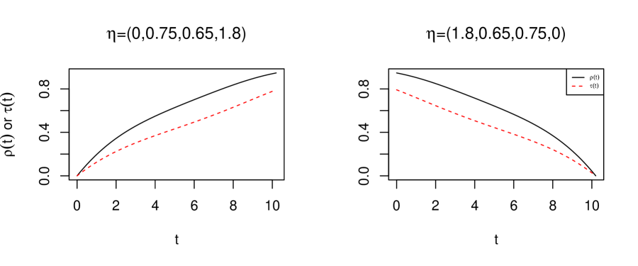
Figure 1: Pearson’s correlation $\rho(t)$ and Kendall’s $\tau(t)$ by the corresponding coefficient vector $\bm{\eta}.$

Three candidate models used for parameters estimation in the two simulation studies are:

• Bivariate Gaussian copula joint model (GJM): the marginals are correctly specified as (11) and (12), while the correlation between the two sub-models after conditioning on the random effects is introduced by the bivariate Gaussian copula function and modelled by 4 order 4 B-spline basis functions over [0,10.2];

• Bivariate $t4$ copula joint model (T4JM): the marginals are correctly specified as (11) and (12), while the correlation between the two sub-models after conditioning on the random effects is introduced by the bivariate $t$ copula function with 4 degrees of freedom and modelled by 4 order 4 B-spline basis functions over [0,10.2];

• Regular joint model (RJM): the marginals are correctly specified and assumed to be conditionally independent given the random effects, which is equivalent to $\rho(t)=0$ or $\tau(t)=0$ under the GJM.

The results of the three fitted models are summarised in Tables (3.1) and (3.2), where SE and SD denote the model-based standard errors from the inverse Hessian matrix and the empirical standard deviations from the $N=500$ Monte Carlo samples, respectively, while CP and ECP represent the coverage probabilities from the model-based and empirical 95% confidence intervals by $\pm 1.96$SE and $\pm 1.96$SD, respectively. The root mean square error of parameter $\theta$ is defined as $RMSE(\theta)=\sqrt{\frac{1}{N}\sum_{i=1}^{N}\left(\hat{\theta}_{i}-\theta\right)^{2}},$ where $\hat{\theta}_{i}$ is the parameter estimate for the $i$th sample.

3.1 Simulation study 1

In simulation study 1, the true datasets are generated by the GJM. Table 3.1 summarises the outputs of simulation study 1. When the model is correctly specified as the GJM, the parameters are generally accurately estimated with low biases. The small discrepancies between RMSE and SD also mean small biases. The values of SE and SD are generally close while the values of CP and ECP are around the nominal value of 0.95. The impact of misspecification of the bivariate Gaussian copula function to the bivariate $t$ copula is very minimal on parameter estimation, observing similar unbiased outputs as in the GJM. However, if the RJM model is fitted, some biases can be observed in $\beta_{11},$ $\alpha$ and the regression parameters in the survival sub-model and this is somehow more obvious under the decreasing correlation pattern. The reason for this may be there are more events in the earlier stages and ignoring the strong correlation from the copula functions at this stage may result in more information loss, compared to the increasing correlation scenario which assumes a weaker correlation at the initial stage. On the other hand, biases for the remaining parameters are quite low. The estimation of $\rho(t)$ can be easily obtained by the approach in Section 2.3, while the confidence band functions can be calculated through the delta method from the variance-covariance matrix of $\hat{\bm{\eta}}$ in the estimating process. However, to make sure the confidence band functions of $\hat{\rho}(t)$ are within $[1,1],$ the confidence band functions of $\hat{r}(t)$ is calculated first and then transformed back to those of $\hat{\rho}(t),$ resulting in asymmetric confidence band functions. Figure 2 depicts the estimated $\rho(t)$ in (red) dashed lines and its corresponding confidence interval functions in (red) dotted lines for the GJM and T4JM under the two correlation patterns. When the copula function is correctly specified as the bivariate Gaussian copula, the estimated $\rho(t)$ functions almost overlap with the true correlation function and the coverage probability functions of the 95% confidence bands are close to the nominal level. When the copula function is misspecified as the bivariate $t$ copula, we observe some departure of the fitted $\rho(t)$ functions from the true correlation function around the range of $2<t<8$ and a deviation of the coverage probability function from the nominal line of 0.95 in the same range. In terms of AIC and BIC, the GJM outperforms the T4JM in 489 and 490 out of the 500 Monte Carlo samples in the increasing and decreasing correlation structure, respectively. Both the GJM and T4JM have better performance than the RJM in all 500 Monte Carlo samples.

Estimation of the parameters by the GJM, T4JM and RJM when the true dataset are generated by the GJM. True $\beta_{10}$ $\beta_{11}$ $\beta_{12}$ $\beta_{13}$ $\beta_{14}$ $\beta_{15}$ $\beta_{21}$ $\beta_{22}$ $\beta_{23}$ $\beta_{24}$ $D_{11}$ $D_{22}$ $D_{12}$ $\sigma$ $\alpha$ value 10 -0.5 1 0.5 0.5 1 -2 -1 -1.5 -2 2 0.2 -0.1 2 -0.5 Increasing correlation with $\bm{\eta}=(0,0.75,0.65,1.8)$ GJM 1-16 Est. 10.022 -0.495 0.993 0.492 0.496 0.979 -2.045 -1.030 -1.532 -2.039 1.920 0.200 -0.097 1.999 -0.510 SE 0.335 0.026 0.236 0.236 0.351 0.323 0.215 0.192 0.272 0.260 0.305 0.030 0.074 0.030 0.035 SD 0.330 0.026 0.245 0.242 0.345 0.328 0.240 0.198 0.293 0.276 0.326 0.029 0.078 0.028 0.040 RMSE 0.331 0.027 0.245 0.242 0.345 0.328 0.244 0.200 0.294 0.278 0.335 0.029 0.078 0.028 0.041 CP 0.954 0.958 0.954 0.946 0.946 0.952 0.918 0.936 0.918 0.930 0.910 0.954 0.934 0.968 0.926 ECP 0.948 0.952 0.958 0.952 0.950 0.956 0.934 0.942 0.948 0.948 0.946 0.958 0.952 0.952 0.938 1-16 T4JM 1-16 Est. 10.024 -0.500 0.993 0.493 0.500 0.983 -2.015 -1.015 -1.509 -2.009 1.928 0.201 -0.099 2.007 -0.502 SE 0.336 0.026 0.237 0.237 0.352 0.324 0.209 0.187 0.266 0.254 0.305 0.030 0.074 0.030 0.034 SD 0.332 0.028 0.247 0.244 0.346 0.329 0.239 0.200 0.295 0.275 0.325 0.029 0.078 0.029 0.039 RMSE 0.333 0.028 0.247 0.244 0.345 0.329 0.239 0.200 0.295 0.275 0.332 0.029 0.078 0.029 0.039 CP 0.944 0.936 0.944 0.942 0.938 0.952 0.920 0.936 0.920 0.926 0.920 0.960 0.936 0.952 0.886 ECP 0.946 0.950 0.952 0.952 0.944 0.952 0.944 0.944 0.948 0.946 0.948 0.956 0.954 0.948 0.938 1-16 RJM 1-16 Est. 10.045 -0.510 0.995 0.494 0.501 0.983 -2.218 -1.112 -1.616 -2.172 1.981 0.227 -0.124 1.992 -0.637 SE 0.336 0.033 0.237 0.236 0.352 0.324 0.297 0.262 0.348 0.333 0.308 0.035 0.079 0.030 0.067 SD 0.330 0.031 0.246 0.241 0.347 0.330 0.312 0.251 0.351 0.322 0.327 0.032 0.082 0.029 0.066 RMSE 0.333 0.033 0.246 0.240 0.346 0.330 0.381 0.274 0.369 0.365 0.327 0.042 0.086 0.030 0.152 CP 0.954 0.948 0.950 0.940 0.944 0.948 0.896 0.942 0.936 0.938 0.938 0.956 0.950 0.944 0.482 ECP 0.948 0.940 0.958 0.956 0.944 0.956 0.888 0.918 0.930 0.926 0.962 0.870 0.952 0.940 0.480 Decreasing correlation with $\bm{\eta}=(1.8,0.65,0.75,0)$ GJM 1-16 Est. 10.000 -0.494 1.001 0.503 0.510 0.980 -2.019 -1.003 -1.527 -2.032 1.930 0.199 -0.100 2.000 -0.506 SE 0.333 0.031 0.236 0.235 0.350 0.323 0.232 0.207 0.279 0.264 0.298 0.030 0.073 0.030 0.048 SD 0.355 0.031 0.252 0.239 0.365 0.342 0.238 0.209 0.293 0.286 0.306 0.031 0.077 0.032 0.049 RMSE 0.355 0.031 0.252 0.239 0.364 0.342 0.238 0.208 0.294 0.288 0.313 0.031 0.077 0.032 0.050 CP 0.930 0.948 0.938 0.952 0.948 0.932 0.948 0.944 0.950 0.934 0.914 0.930 0.942 0.942 0.956 ECP 0.954 0.954 0.950 0.958 0.958 0.946 0.956 0.948 0.950 0.950 0.952 0.964 0.954 0.952 0.956 1-16 T4JM 1-16 Est. 10.004 -0.491 0.996 0.504 0.507 0.977 -1.980 -0.987 -1.506 -2.003 1.936 0.199 -0.101 2.005 -0.492 SE 0.332 0.031 0.236 0.235 0.350 0.323 0.226 0.204 0.277 0.259 0.294 0.030 0.073 0.030 0.046 SD 0.356 0.032 0.255 0.241 0.365 0.343 0.236 0.209 0.290 0.287 0.308 0.031 0.077 0.032 0.050 RMSE 0.356 0.033 0.255 0.240 0.364 0.344 0.237 0.209 0.290 0.287 0.314 0.031 0.077 0.032 0.050 CP 0.924 0.940 0.934 0.944 0.942 0.930 0.946 0.944 0.942 0.932 0.902 0.934 0.946 0.938 0.928 ECP 0.952 0.946 0.952 0.958 0.958 0.940 0.950 0.948 0.958 0.956 0.952 0.962 0.958 0.944 0.948 1-16 RJM 1-16 Est. 9.811 -0.533 1.090 0.544 0.588 1.085 -2.362 -1.165 -1.758 -2.351 2.458 0.247 -0.144 1.976 -0.708 SE 0.361 0.032 0.256 0.255 0.378 0.348 0.320 0.282 0.377 0.362 0.372 0.040 0.096 0.030 0.073 SD 0.377 0.033 0.273 0.262 0.391 0.367 0.325 0.279 0.389 0.376 0.399 0.041 0.102 0.031 0.078 RMSE 0.422 0.047 0.287 0.266 0.400 0.376 0.486 0.324 0.466 0.514 0.607 0.063 0.111 0.040 0.222 CP 0.904 0.806 0.924 0.952 0.952 0.930 0.816 0.914 0.904 0.844 0.794 0.854 0.938 0.846 0.142 ECP 0.914 0.828 0.936 0.952 0.954 0.942 0.800 0.906 0.916 0.852 0.782 0.794 0.926 0.882 0.224

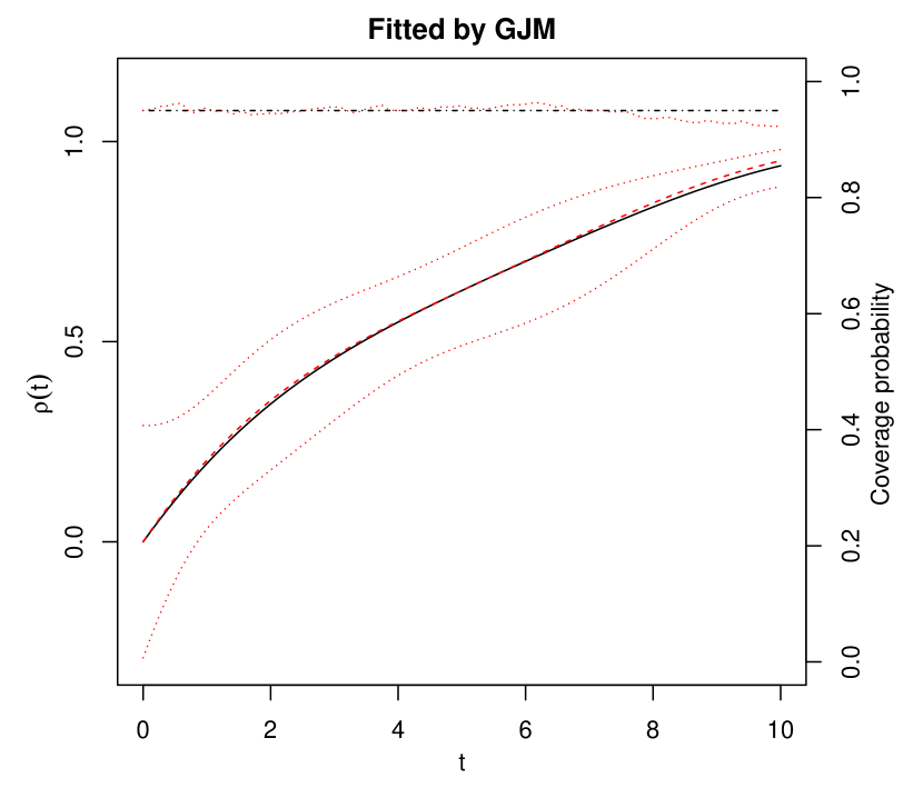
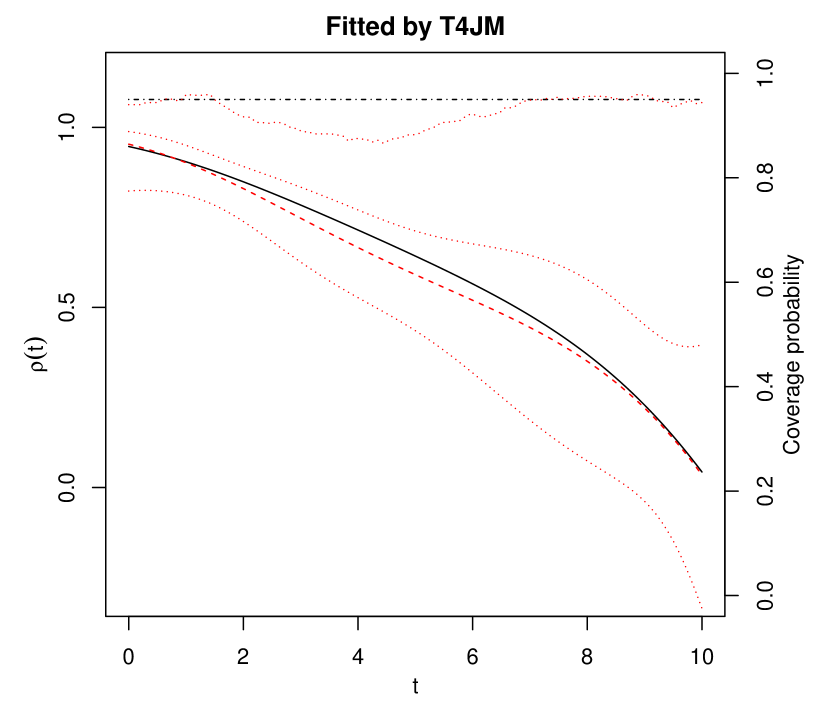
Figure 2: The fitted Pearson’s correlation functions $\hat{\rho}(t)$ (dashed lines) with their corresponding 95% confidence interval functions (dotted lines) by the GJM and T4JM when the true dataset are generated under the GJM. The dotted line at the top of each plot are the coverage probability functions of 95% confidence bands with the nominal reference line at 0.95 in dotted-dash line. The true Pearson’s correlation functions are in solid line.

3.2 Simulation study 2

In simulation study 2, the true datasets are generated by the T4JM. Table 3.2 summarises the outputs of simulation study 2. Similar to the simulation study 1, the correctly specified T4JM and the misspecified GJM both provide quite accurate parameter estimation in terms of bias, SD, SE, RMSE, CP and ECP. However, the misspecified RJM leads to bias in the estimation of $\beta_{11},$ $\alpha$ and the regression parameters in the survival sub-model, similar to the findings in simulation study 1. It is also noticeable that the variance components of the random effects have more significant biases under the decreasing correlation structure in both simulation studies . Figure 3 displays the estimated $\rho(t)$ in (red) dash lines with their corresponding confidence bands in (red) dotted lines, under both the T4JM and GJM. The correctly specified T4JM provides relatively accurate estimation of $\rho(t)$ as expected, however, the estimated $\rho(t)$ provided by the GJM is surprisingly accurate, with low biases and a coverage probability function around the nominal level of 0.95. In fact, T4JM only provides better fitting than GJM in 401 and 444 out of 500 Monte Carlo samples in increasing and decreasing correlation structure in terms of AIC and BIC, respectively, implying a lower power of selecting the correct model compared to simulation study 1. Overall, according to both simulation studies, the GJM provides more robust fitting than the T4JM in parameter estimation, especially for the correlation parameters of the bivariate functional copula, under copula misspecification.

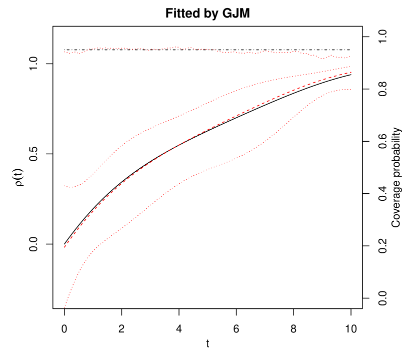
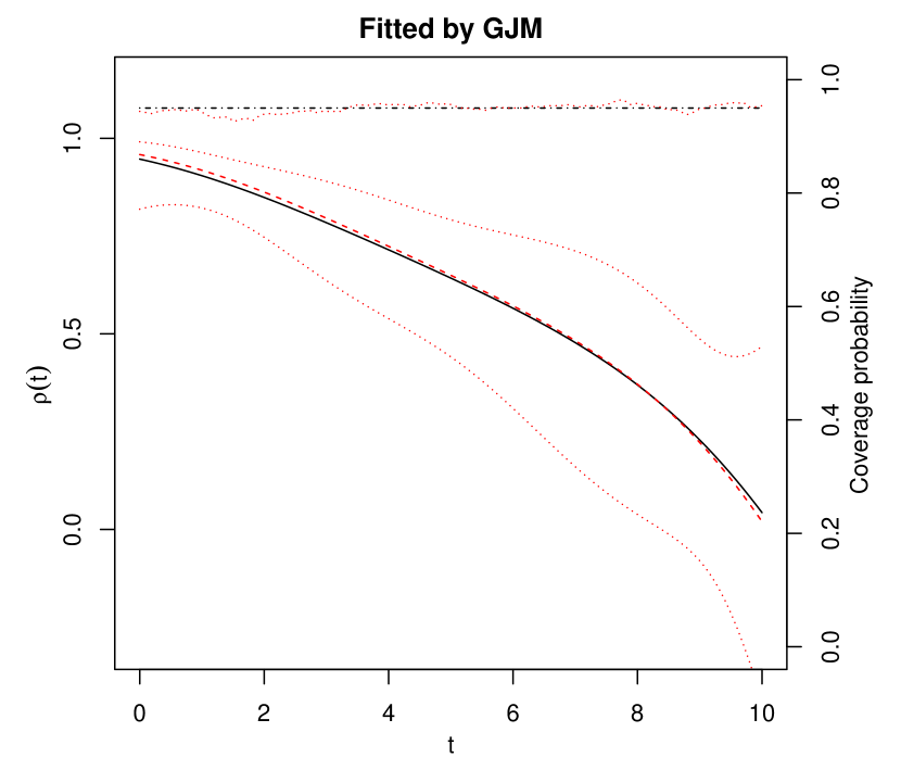
Figure 3: The fitted Pearson’s correlation functions $\hat{\rho}(t)$ (dashed lines) with their corresponding 95% confidence interval functions (dotted lines) by the T4JM and GJM when the true dataset are generated under the T4JM. The dotted line at the top of each plot are the coverage probability functions of 95% confidence bands with the nominal reference line at 0.95 in dotted-dash line. The true Pearson’s correlation functions are in solid line.

Estimation of the parameters by the T4JM, GJM and RJM when the true dataset are generated by the T4JM. True $\beta_{10}$ $\beta_{11}$ $\beta_{12}$ $\beta_{13}$ $\beta_{14}$ $\beta_{15}$ $\beta_{21}$ $\beta_{22}$ $\beta_{23}$ $\beta_{24}$ $D_{11}$ $D_{22}$ $D_{12}$ $\sigma$ $\alpha$ value 10 -0.5 1 0.5 0.5 1 -2 -1 -1.5 -2 2 0.2 -0.1 2 -0.5 Increasing correlation with $\bm{\eta}=(0,0.75,0.65,1.8)$ T4JM 1-16 Est. 9.998 -0.496 0.993 0.500 0.507 0.995 -2.035 -1.016 -1.517 -2.025 1.912 0.200 -0.097 2.003 -0.506 SE 0.335 0.026 0.237 0.236 0.352 0.324 0.208 0.186 0.265 0.253 0.304 0.030 0.073 0.030 0.033 SD 0.345 0.027 0.243 0.255 0.350 0.328 0.226 0.209 0.274 0.248 0.288 0.029 0.070 0.031 0.040 RMSE 0.344 0.027 0.243 0.254 0.350 0.327 0.228 0.210 0.274 0.249 0.300 0.029 0.071 0.031 0.040 CP 0.946 0.946 0.948 0.932 0.956 0.940 0.922 0.928 0.940 0.950 0.934 0.952 0.960 0.944 0.902 ECP 0.950 0.954 0.954 0.946 0.956 0.940 0.944 0.942 0.946 0.944 0.940 0.958 0.958 0.948 0.938 1-16 GJM 1-16 Est. 9.996 -0.496 0.996 0.501 0.504 0.994 -2.041 -1.019 -1.521 -2.032 1.956 0.203 -0.096 1.999 -0.509 SE 0.338 0.027 0.238 0.237 0.355 0.326 0.214 0.191 0.272 0.260 0.311 0.031 0.075 0.030 0.035 SD 0.346 0.027 0.246 0.256 0.354 0.330 0.229 0.213 0.281 0.252 0.296 0.030 0.073 0.031 0.040 RMSE 0.346 0.027 0.246 0.256 0.354 0.330 0.233 0.214 0.281 0.254 0.299 0.030 0.073 0.031 0.041 CP 0.944 0.954 0.952 0.930 0.950 0.940 0.930 0.924 0.938 0.956 0.950 0.962 0.954 0.948 0.920 ECP 0.948 0.960 0.956 0.950 0.954 0.948 0.944 0.950 0.946 0.932 0.954 0.950 0.950 0.954 0.940 1-16 RJM 1-16 Est. 10.022 -0.513 0.996 0.499 0.510 1.001 -2.214 -1.105 -1.615 -2.173 2.009 0.231 -0.122 1.991 -0.639 SE 0.338 0.033 0.239 0.238 0.355 0.327 0.297 0.262 0.350 0.334 0.313 0.036 0.081 0.030 0.068 SD 0.350 0.031 0.247 0.259 0.351 0.331 0.303 0.263 0.340 0.307 0.297 0.034 0.080 0.031 0.066 RMSE 0.350 0.033 0.247 0.259 0.351 0.331 0.371 0.283 0.359 0.352 0.297 0.046 0.083 0.032 0.154 CP 0.946 0.952 0.952 0.928 0.958 0.940 0.900 0.938 0.946 0.960 0.958 0.910 0.950 0.938 0.490 ECP 0.958 0.926 0.962 0.944 0.954 0.950 0.890 0.934 0.926 0.914 0.958 0.844 0.944 0.950 0.482 Decreasing correlation with $\bm{\eta}=(1.8,0.65,0.75,0)$ T4JM 1-16 Est. 9.992 -0.496 1.005 0.494 0.521 1.004 -2.009 -1.010 -1.530 -2.022 1.915 0.199 -0.095 2.002 -0.508 SE 0.331 0.030 0.234 0.233 0.348 0.319 0.225 0.204 0.276 0.259 0.288 0.030 0.072 0.030 0.046 SD 0.365 0.031 0.240 0.244 0.385 0.338 0.241 0.201 0.291 0.261 0.316 0.028 0.076 0.030 0.054 RMSE 0.365 0.032 0.240 0.244 0.385 0.338 0.241 0.201 0.292 0.261 0.327 0.028 0.077 0.030 0.054 CP 0.918 0.946 0.936 0.946 0.924 0.930 0.934 0.960 0.932 0.944 0.928 0.936 0.940 0.956 0.916 ECP 0.954 0.962 0.940 0.954 0.942 0.938 0.946 0.950 0.938 0.940 0.952 0.958 0.946 0.958 0.954 1-16 GJM 1-16 Est. 9.992 -0.497 1.008 0.496 0.517 1.003 -2.023 -1.015 -1.531 -2.027 1.919 0.201 -0.095 2.000 -0.513 SE 0.334 0.030 0.236 0.235 0.350 0.322 0.232 0.208 0.280 0.264 0.295 0.031 0.073 0.030 0.049 SD 0.354 0.032 0.240 0.241 0.370 0.327 0.241 0.207 0.293 0.266 0.316 0.029 0.078 0.030 0.056 RMSE 0.354 0.032 0.240 0.241 0.370 0.326 0.242 0.208 0.295 0.267 0.326 0.029 0.078 0.030 0.057 CP 0.930 0.952 0.940 0.950 0.932 0.940 0.942 0.962 0.930 0.942 0.908 0.940 0.942 0.954 0.924 ECP 0.946 0.958 0.948 0.952 0.948 0.954 0.950 0.948 0.940 0.942 0.958 0.956 0.952 0.956 0.948 1-16 RJM 1-16 Est. 9.811 -0.536 1.098 0.534 0.596 1.098 -2.375 -1.181 -1.783 -2.360 2.446 0.250 -0.135 1.975 -0.723 SE 0.362 0.032 0.256 0.255 0.378 0.348 0.324 0.287 0.384 0.368 0.370 0.041 0.096 0.030 0.074 SD 0.387 0.035 0.261 0.256 0.404 0.366 0.332 0.276 0.390 0.357 0.403 0.039 0.104 0.030 0.088 RMSE 0.430 0.049 0.279 0.258 0.415 0.379 0.500 0.329 0.482 0.507 0.601 0.064 0.109 0.039 0.240 CP 0.906 0.794 0.924 0.962 0.924 0.932 0.818 0.926 0.898 0.856 0.816 0.866 0.940 0.858 0.116 ECP 0.918 0.804 0.930 0.958 0.930 0.948 0.806 0.898 0.876 0.818 0.806 0.766 0.938 0.864 0.298

3.3 Dynamic prediction

After a joint model is fitted, we also focus on predictions of the subject-specific survival probabilities based on some baseline covariates and updated longitudinal information. The quality of the predictions is of interest as well and can be assessed by some metrics like the area under the receiver operating characteristics curve (AUC) and prediction error (PE).

3.3.1 Formula for prediction

Suppose a functional bivariate copula joint model is fitted based on a random sample of $n$ subjects $\mathcal{\bm{D}}_{n}=\left\{T_{i},\delta_{i},\bm{y}_{i};i=1,...,n\right\}.$ Predictions of survival probabilities at time $u>t$ for a new subject $i,$ which has $j,$ $1\leq j\leq n_{i},$ longitudinal measurements $\mathcal{\bm{Y}}_{i}(t)=\left\{y_{i}(s);0\leq s<t\right\}$ up to $t$ and a vector of baseline covariates $\bm{w}_{i},$ can be easily derived from (5) and (8) as:

$$\pi_{i}(u|t) = P(T_{i}^{*}>u|T_{i}^{*}>t,\mathcal{\bm{Y}}_{i}(t),\bm{w}_{i},\mathcal{\bm{D}}_{n};\bm{\theta})=P(T_{i}^{*}>u|T_{i}^{*}>t,\mathcal{\bm{Y}}_{i}(t),\bm{w}_{i};\bm{\theta})$$ (13)

$$= \int_{R^{q}}P(T_{i}^{*}>u|T_{i}^{*}>t,\mathcal{\bm{Y}}_{i}(t),\bm{w}_{i},\bm{b}_{i};\bm{\theta})f_{\bm{b}_{i}}(\bm{b}_{i}|T_{i}^{*}>t,\mathcal{\bm{Y}}_{i}(t),\bm{w}_{i};\bm{\theta})d\bm{b}_{i}$$

$$= \int_{R^{q}}\frac{S_{T_{i}^{*}}\left(u|T_{i}^{*}>s_{ij},\mathcal{\bm{Y}}_{i}(t),\bm{w}_{i},\bm{b}_{i};\bm{\theta}\right)}{S_{T_{i}^{*}}\left(t|T_{i}^{*}>s_{ij},\mathcal{\bm{Y}}_{i}(t),\bm{w}_{i},\bm{b}_{i};\bm{\theta}\right)}f_{\bm{b}_{i}}(\bm{b}_{i}|T_{i}^{*}>t,\mathcal{\bm{Y}}_{i}(t),\bm{w}_{i};\bm{\theta})d\bm{b}_{i}.,$$

The integral in (13) can be approximated by its first-order estimate (Rizopoulos, 2011[31]) using the empirical Bayes estimate for $\bm{b}_{i}:$

$$\hat{\pi}_{i}(u|t)\approx\frac{S_{T_{i}^{*}}\left(u|T_{i}^{*}>s_{ij},\mathcal{\bm{Y}}_{i}(t),\bm{w}_{i},\hat{\bm{b}}_{i};\hat{\bm{\theta}}\right)}{S_{T_{i}^{*}}\left(t|T_{i}^{*}>s_{ij},\mathcal{\bm{Y}}_{i}(t),\bm{w}_{i},\hat{\bm{b}}_{i};\hat{\bm{\theta}}\right)},$$ (14)

where $\hat{\bm{\theta}}$ denotes the maximum likelihood estimators and $\hat{\bm{b}}_{i}$ denotes the mode of the conditional distribution $f_{\bm{b}_{i}}(\bm{b}_{i}|T_{i}^{*}>t,\mathcal{\bm{Y}}_{i}(t),\bm{w}_{i};\bm{\theta}).$

For the bivariate Gaussian copula, (14) becomes

$$\hat{\pi}_{i}(u|t)\approx\Phi\left(-\frac{Z_{u|\hat{\bm{b}}_{i},s_{ij}}-\hat{\rho}(s_{ij})Z_{y_{ij}|\hat{\bm{b}}_{i},s_{ij}}}{\sqrt{1-\hat{\rho}(s_{ij})^{2}}}\right)\div\Phi\left(-\frac{Z_{t|\hat{\bm{b}}_{i},s_{ij}}-\hat{\rho}(s_{ij})Z_{y_{ij}|\hat{\bm{b}}_{i},s_{ij}}}{\sqrt{1-\hat{\rho}(s_{ij})^{2}}}\right),$$ (15)

which reduces to $\displaystyle\frac{S_{T_{i}^{*}}\left(u|\bm{w}_{i},\hat{\bm{b}}_{i};\hat{\bm{\theta}}\right)}{S_{T_{i}^{*}}\left(t|\bm{w}_{i},\hat{\bm{b}}_{i};\hat{\bm{\theta}}\right)}=\displaystyle\mbox{exp}\left\{-\int_{t}^{u}h_{i}(s|\bm{w}_{i},\hat{\bm{b}}_{i};\hat{\bm{\theta}})ds\right\}$ given $\rho(t)$ is a constant function of 0.

For the bivariate $t$ copula,

$$\hat{\pi}_{i}(u|t) \approx \Psi\left(-\frac{W_{u|\hat{\bm{b}}_{i},s_{ij}}-\hat{\rho}(s_{ij})W_{y_{ij}|\hat{\bm{b}}_{i},s_{ij}}}{\hat{\sigma}(s_{ij}|\hat{\bm{b}}_{i},s_{ij})};\nu+1\right)$$ (16)

$$\div \Psi\left(-\frac{W_{t|\hat{\bm{b}}_{i},s_{ij}}-\hat{\rho}(s_{ij})W_{y_{ij}|\hat{\bm{b}}_{i},s_{ij}}}{\hat{\sigma}(s_{ij}|\hat{\bm{b}}_{i},y_{ij})};\nu+1\right).$$

3.3.2 Assessment of prediction performance

The overall performance of the model in predicting survival probabilities are evaluated in terms of discrimination by AUC and calibration by PE. Consider a pair of randomly selected subjects at risk by $t$, denoted as $i_{1}$ and $i_{2}$, from the population. Suppose subject $i_{1}$ experiences the event in the interval $(t,u]$ whereas subject $i_{2}$ does not. A good predictive model is supposed to assign higher predicted survival probabilities to subject $i_{2}$ than subject $i_{1}$ (Garre et al., 2008[11]). The AUC defined as:

$$\mbox{AUC}(u|t)=P\left\{\pi_{i_{2}}(u|t)>\pi_{i_{1}}(u|t)|T_{i_{2}}^{*}>u,t<T_{i_{1}}^{*}\leq u\right\}$$

is a popular tool to assess the discriminative performance of the model. An AUC value closer to 1 implies a better discriminative capability of the model. On the other hand, if a subject $i$ is event free up to time $u,$ an accurate predicting model is expected to provide $\pi_{i}(u|t)$ close to 1 and close to 0 otherwise. The PE, or the Brier score, defined as:

$$\mbox{PE}(u|t)=E\left[\left\{I(T_{i}^{*}>u)-\pi_{i}(u|t)\right\}^{2}|T_{i}^{*}>t\right]$$

is a common approach to calibrate the predictive accuracy of the model. A model with a smaller PE value (closer to 0) is preferable. To account for censoring in the population, the weighted AUC and PE estimators from Andrinopoulou et al. (2018)[3] are adopted.

We simulate $N=100$ new Monte Carlo datasets each with sample size $n=200$ under the same parameter settings as in simulation studies 1 and 2 with longitudinal measurements scheduled at time points $t=1,2,...,10.$ The dynamic $\mbox{AUC}(u|t)$ and $\mbox{BS}(u|t)$ are evaluated at $t=1,3,$ and 5 with $\Delta t=u-t=1$ for the three candidate models.

From Figures 4 and 6, under the increasing correlation pattern, all three candidate models have similar discriminative capability and predictive accuracy at $t=1,$ while the GJM and T4JM have much better predictive performances than the RJM, providing much higher AUCs and lower PEs at $t=9$. Figures 5 and 7 present the opposite pattern, as the correlation function is decreasing in this instance. For both correlation structures, the GJM and T4JM have similar performance, even if one of the copula functions is misspecified. The bivariate functional copula joint model generally offers significant improvement compared with the RJM, especially when the correlation is strongest.

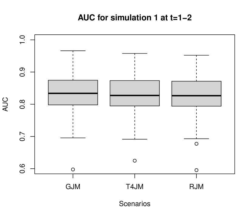
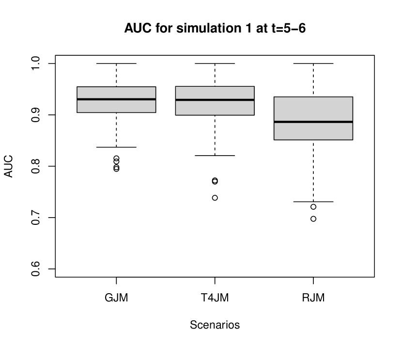
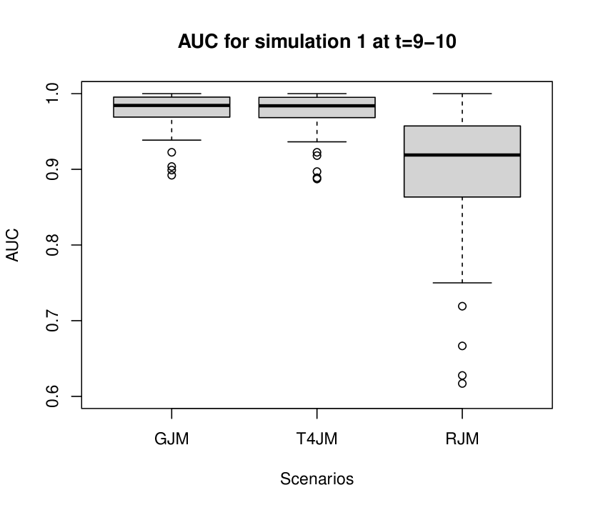
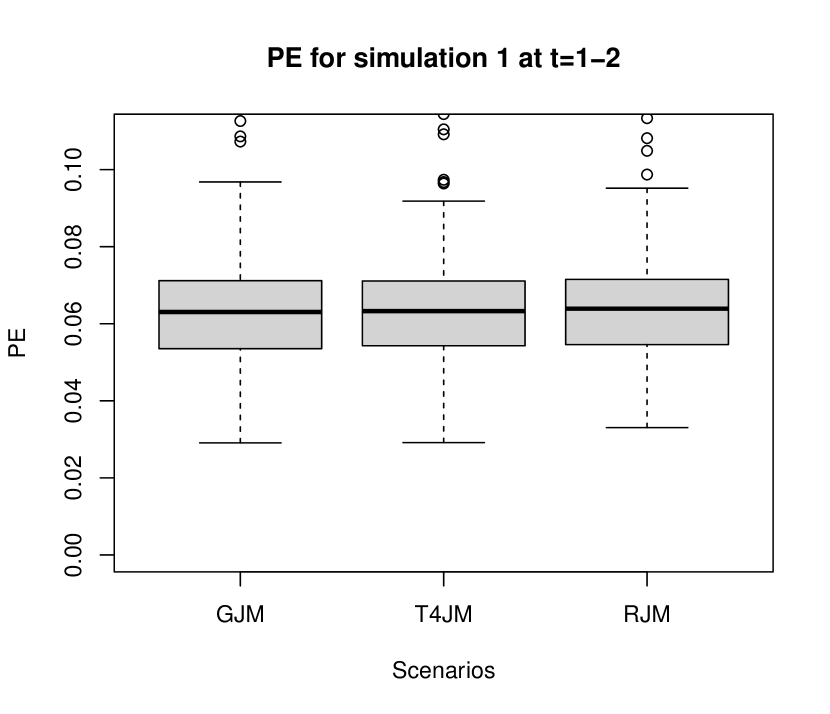
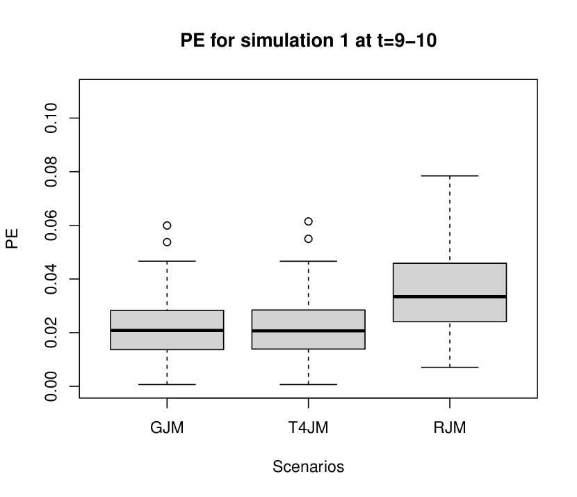
Figure 4: The dynamic AUC$(t+\Delta t|t)$ and PE$(t+\Delta t|t)$ at $t=$1, 5 and 9 with $\Delta t=1$ by the GJM, T4JM and RJM from 100 new Monte Carlo samples with sample size $n=200$ from the simulation study 1 with increasing correlation function.

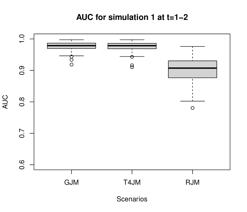
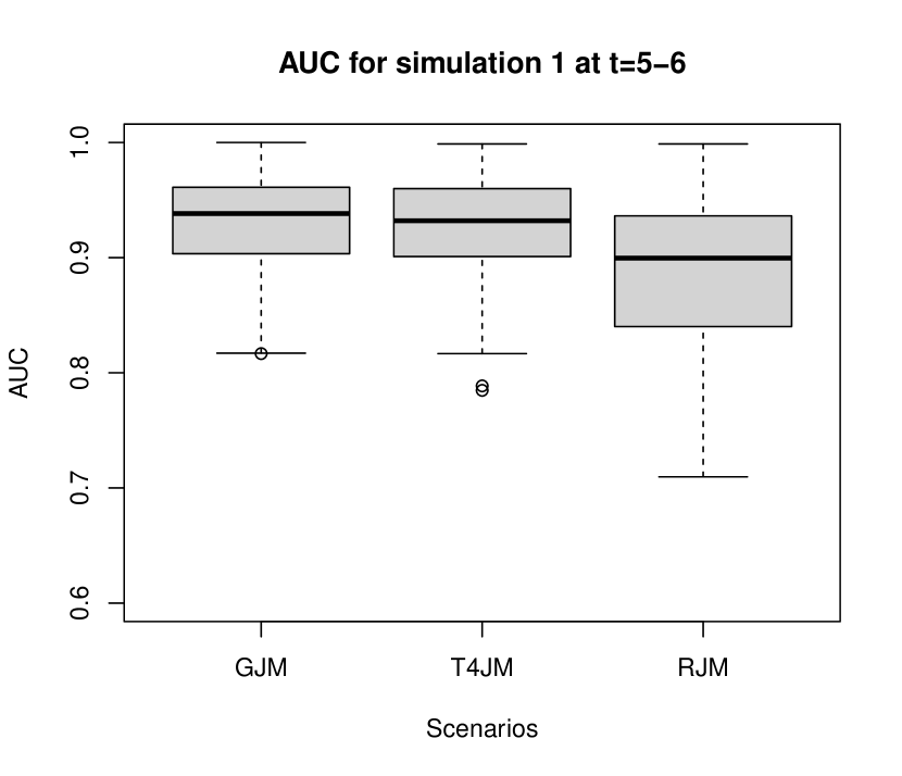
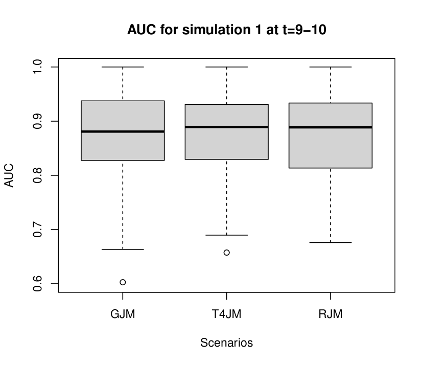
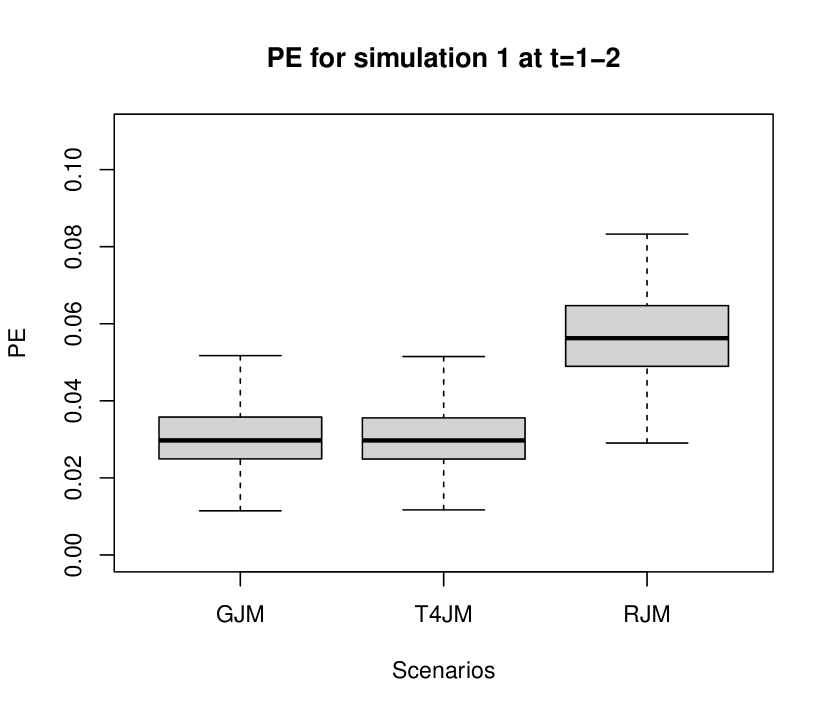
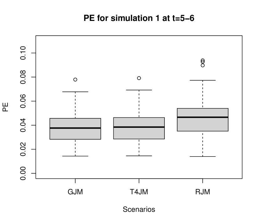
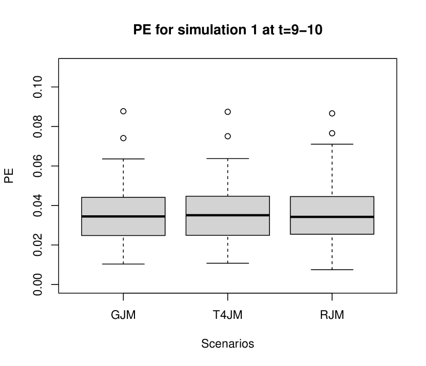
Figure 5: The dynamic AUC$(t+\Delta t|t)$ and PE$(t+\Delta t|t)$ at $t=$1, 5 and 9 with $\Delta t=1$ by the GJM, T4JM and RJM from 100 new Monte Carlo samples with sample size $n=200$ from the simulation study 1 with decreasing correlation function.

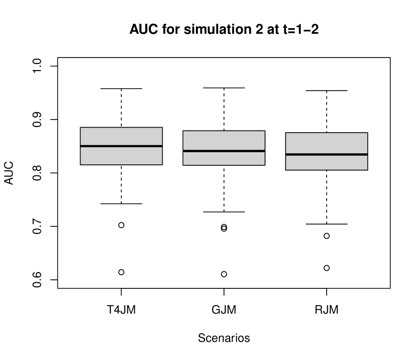
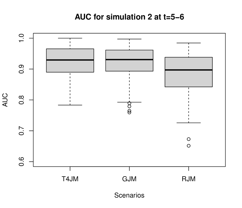
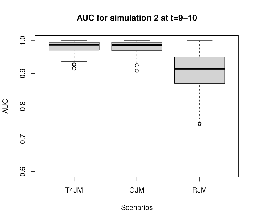
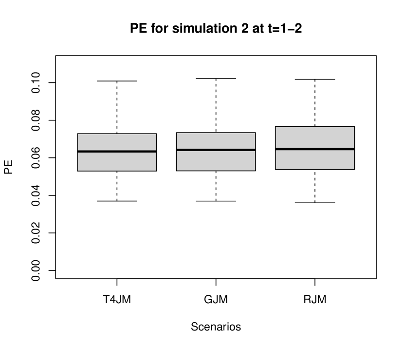
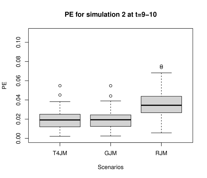
Figure 6: The dynamic AUC$(t+\Delta t|t)$ and PE$(t+\Delta t|t)$ at $t=$1, 5 and 9 with $\Delta t=1$ by the T4JM, GJM and RJM from 100 new Monte Carlo samples with sample size $n=200$ from the simulation study 2 with increasing correlation function.

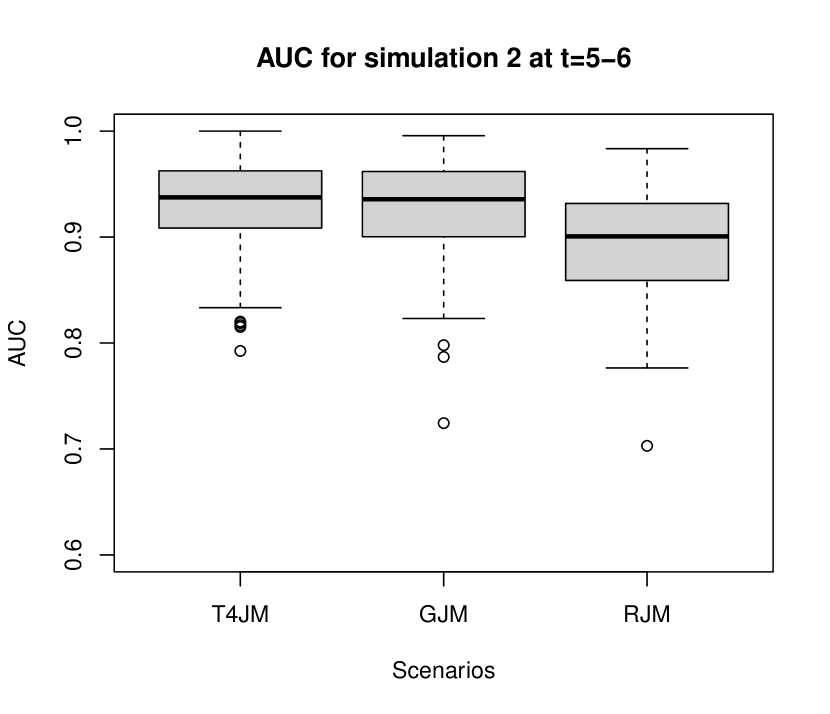
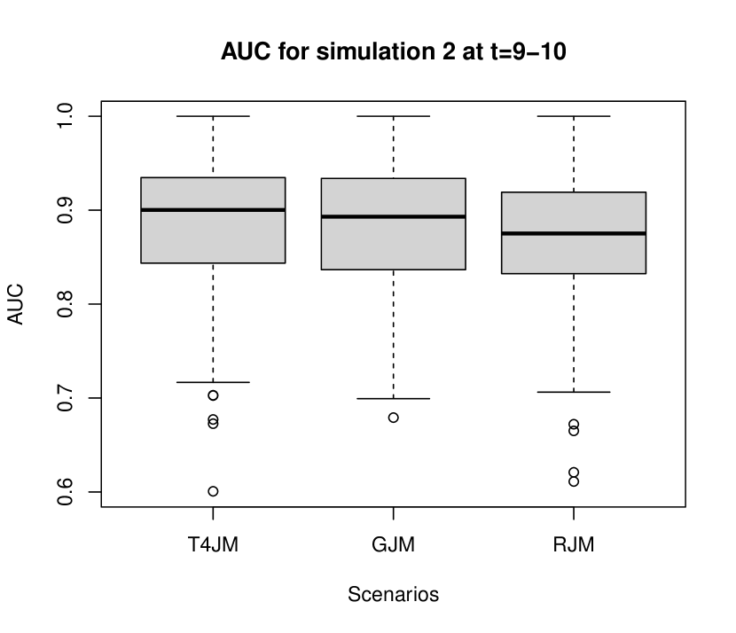
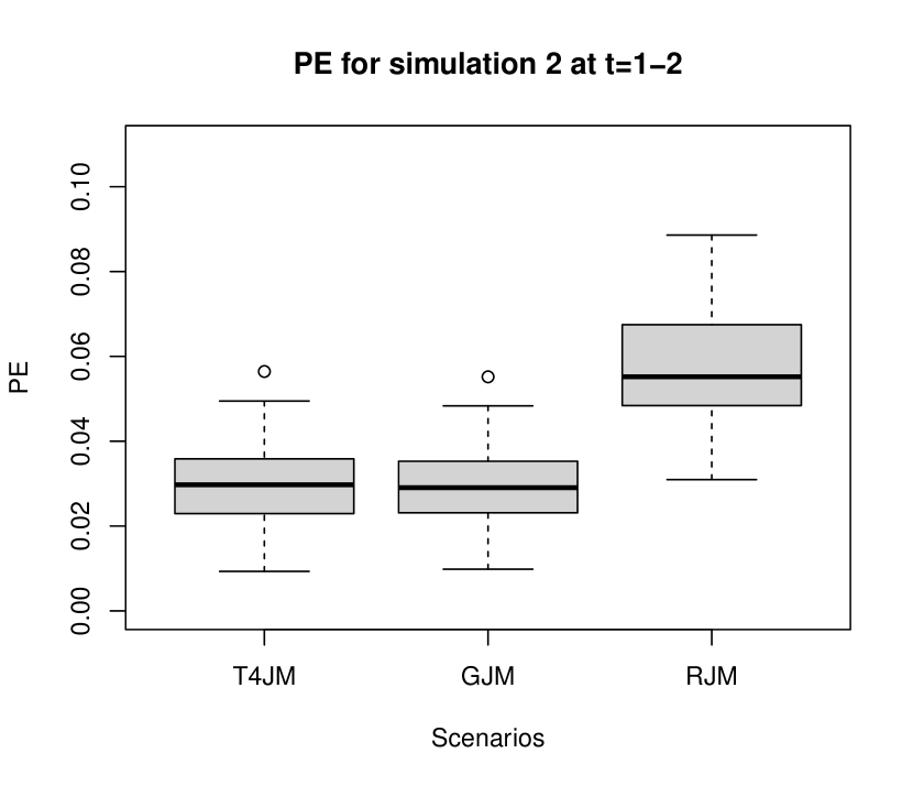
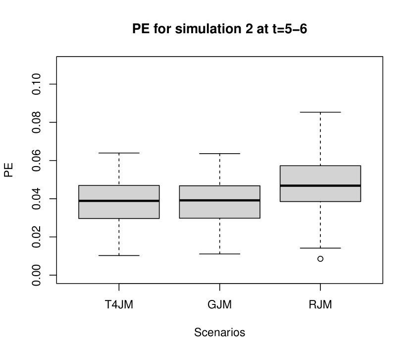
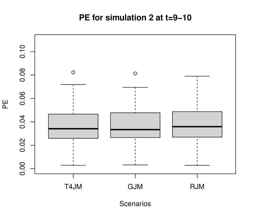
Figure 7: The dynamic AUC$(t+\Delta t|t)$ and PE$(t+\Delta t|t)$ at $t=$1, 5 and 9 with $\Delta t=1$ by the T4JM, GJM and RJM from 100 new Monte Carlo samples with sample size $n=200$ from the simulation study 2 with decreasing correlation function.

Although AIC and BIC can detect the best model among the candidates, as demonstrated earlier, the bivariate functional Gaussian joint model, which is computationally easier compared with the bivariate functional $t$ copula joint model, is still a good choice in terms of both parameter estimation and survival probability prediction if, in practice, the correct model is unknown.

4 Application to the PBC data

The PBC data (Murtaugh, et al, 1994[26]) records the information of 312 patients with primary biliary cirrhosis from 1974 to 1984. The main task of this study is to evaluate the treatment effect of D-penicillamine (158 randomised patients) compared with placebo (154 randomised patients). Baseline covariates such as age at the entry of study, gender and treatment are recorded. In the meanwhile, several biomarkers, such as serum bilirubin level (mg/dl), the presence of spiders and hepatomegaly (indicator variables), are monitored as follow-up. Among them, the serum bilirubin level is considered as a stronger indicator for the progression of the disease. After the baseline measurement, each patient was scheduled for visits at six months, one year and yearly afterwards, but not all patients attended the appointments at the scheduled time points and some even missed appointments, leading to an unbalanced dataset. Also due to death and censoring, only 1945 measurements of serum bilirubin levels are recorded, with the maximum measurement time up to 14.106 years and the number of measurements for each patient vary from 1 to 16. By the end of study, 149 patients died, 29 had a transplantation and 143 were still alive.

The proposed functional bivariate copula joint model with random effects is used to model the PBC data, with the longitudinal process specified as follows:

$$y_{ij}=\mu(s_{ij})+\beta_{11}drug_{i}+\beta_{12}sex_{i}+\beta_{13}age_{i}+b_{i0}+b_{i1}s_{ij}+\varepsilon_{ij},$$ (17)

where $\varepsilon_{ij}\sim N\left(0,\sigma^{2}\right),$ $(b_{i0},b_{i1})\sim N\left(0,\bm{D}\right)$ and $y_{ij}$ is the logarithm of serum bilirubin level for the $i$th subject at time $s_{ij}.$ Unlike in the simulation study, we model the population mean function $\mu(t)$ non-linearly by B-spline basis functions to allow more flexibility. Death or transplantation is defined as the composite event. The time to event process is specified as:

$$h_{i}(t)=h_{0}(t)\mbox{exp}\left\{\beta_{21}drug_{i}+\beta_{22}sex_{i}+\beta_{23}age_{i}+\alpha\left(b_{i0}+b_{i1}t\right)\right\},$$ (18)

where $drug_{i}=1$ for D-penicillamine, $gender_{i}=1$ for female and $h_{0}(t)$ is a piecewise-constant function with some equally spaced knots between 0 and the maximum observed event time at 14.306.

Parameter estimations based on PBC data for three candidate models. PRJM PGJM PTJM (Con. Independent) (Gaussian copula) ($t$ copula with $df=11$) Est. SE Est. SE Est. SE $\beta_{11}$ -0.132 0.111 -0.131 0.112 -0.134 0.112 $\beta_{12}$ -0.161 0.171 0.195 0.165 -0.200 0.165 $\beta_{13}$ -0.0005 0.005 0.000 0.005 0.002 0.005 $\beta_{21}$ -0.213 0.224 -0.166 0.211 -0.172 0.214 $\beta_{22}$ -0.148 0.307 -0.175 0.260 -0.156 0.261 $\beta_{23}$ 0.042 0.011 0.045 0.005 0.047 0.005 $D_{11}$ 0.962 0.082 0.969 0.083 0.968 0.083 $D_{22}$ 0.038 0.005 0.033 0.005 0.032 0.004 $D_{12}$ 0.083 0.016 0.071 0.016 0.070 0.015 $\sigma$ 0.344 0.007 0.343 0.007 0.344 0.007 $\alpha$ 1.319 0.100 1.234 0.081 1.235 0.084 Loglik -1936.456 -1897.908 -1896.607 AIC 3916.912 3849.817 3847.214 BIC 3999.258 3950.878 3948.275

Three candidate models are proposed for fitting the PBC dataset:

• The bivariate Gaussian copula joint model (PGJM): the two sub-models are specified as (17) and (18), while the correlation between them is introduced by the bivariate Gaussian copula;

• The bivariate $t$ copula joint model (PTJM): the two sub-models are specified as (17) and (18), while the correlation between them is introduced by the bivariate $t$ copula function with the $df$ to be selected;

• Regular joint model (PRJM): the two sub-models are specified as (17) and (18) and assumed to be conditionally independent given the random effects, which is equivalent to $\tau(t)=0$ and $\rho(t)=0$ in the Gaussian joint model.

We select the optimal number of B-spline basis functions and piecewise-constant baseline hazard function by AIC and BIC, and the optimal combination is 4 B-spline basis functions of order 4 for $\mu(t),$ 5 B-spline basis functions of order 5 for $\rho(t)$ and a piecewise-constant baseline function with 7 pieces. We also notice that the fitted trajectories of $\mu(t)$ and $\rho(t)$ remain approximately the same when increasing the numbers and orders of the B-splines function, while there some significant changes in the trajectories by decreasing the numbers and orders. When fitting the PTJM, the maximum of the log-likelihood value is reached at $df=11.$ The fitted results of the three candidate models are summarised in Table 4. The two copula joint models provide similar fits in terms of parameter estimation and they result in a similar fitted population mean function $\mu(t)$ and Pearson’s correlation function $\rho(t),$ according to Figures 8 and 9. In addition, the two copula joint models both provide significantly better fitting than the PRJM in terms of AIC and BIC. This result is also consistent with the likelihood ratio or Wald test between the PRJM and PGJM. The correlation between the two sub-models is stronger during $1\leq t\leq 2$ and $7\leq t\leq 10$, while it is close to 0 during $3\leq t\leq 7$ and the confidence intervals are much wider, especially for PTJM, after $t=11,$ as there are fewer data beyond this point. We also notice that the fitted mean function $\mu(t)$ of the regular joint model is higher than that of the copula joint models as $t$ increases, although they are fairly close in the earlier stages. Again, the confidence intervals of the mean functions are obviously larger after $t=11$ for all three joint models, due to sparser observations.

As the visit is scheduled yearly after the first year, the AUC and PE are calculated for the follow-up times $t=1,...,10$ with $\Delta t=1$ by leave-one-out cross-validation. The results are summarised in Table 4. When the correlation is weak between the two sub-models, such as when $3\leq t\leq 7,$ the discriminative performance of the three candidates models are similar, with PRJM sometimes even having best performance, e.g. at $t=4$ and 5. When the correlation between the two sub-models is strong, for example at $t=8,$ 9 and 10, the two copula joint models have significantly better performance than the PRJM. The calculation of AUC and PE values are terminated for $t\geq 11$ as there are only three events beyond this time point. Generally, the copula joint model provides a better prediction by utilising the information in the residuals and the choice of copula function is of less importance. The bivariate Gaussian copula joint model is recommended in practice as it require less computation.

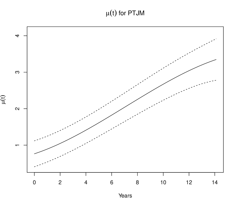
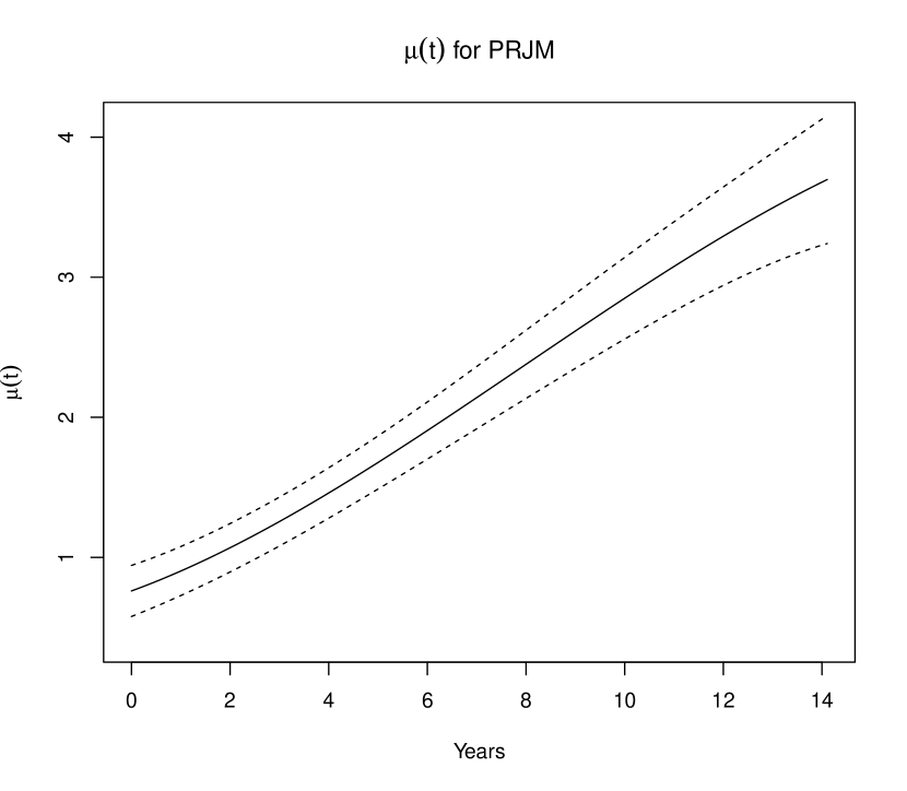
Figure 8: The fitted mean functions $\mu(t)$ for PBC dataset by the PGJM, PTJM with $df=11$ and PRJM with the corresponding 95% confidence band (dashed lines).

AUC and PE for three candidate models at different timepoints with $\Delta t=$1 for the PBC dataset. $t=1$ $t=2$ $t=3$ $t=4$ $t=5$ $t=6$ $t=7$ $t=8$ $t=9$ $t=10$ AUC($t+\Delta t|t$) 1-11 PGJM 0.772 0.928 0.857 0.846 0.729 0.870 0.799 0.774 0.880 0.941 PTJM 0.764 0.927 0.849 0.846 0.745 0.880 0.792 0.772 0.873 0.928 PRJM 0.739 0.927 0.847 0.851 0.766 0.878 0.791 0.751 0.796 0.876 1-11 PE($t+\Delta t|t$) 1-11 PGJM 0.041 0.069 0.060 0.060 0.064 0.078 0.049 0.105 0.089 0.068 PTJM 0.042 0.067 0.059 0.060 0.064 0.078 0.052 0.108 0.091 0.070 PRJM 0.043 0.068 0.058 0.062 0.064 0.077 0.054 0.109 0.107 0.097

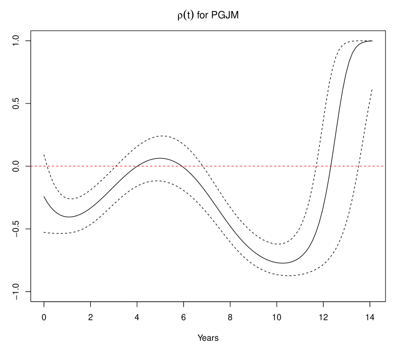
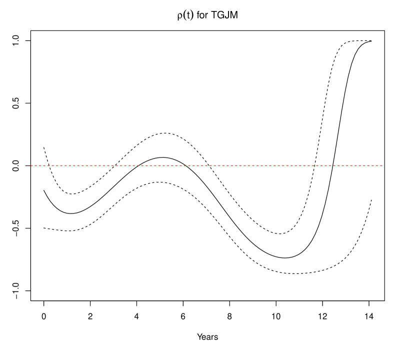
Figure 9: The fitted Pearson’s correlation functions $\rho(t)$ for PBC dataset by the PGJM model and PTJM with $df=11$ with the corresponding 95% confidence band (dashed lines) and reference lines (horizontal dashed lines) at zero.

Figure 10 displays the predicted survival probabilities of subject 21 from the PBC dataset at $t=8.017,$ 9.008 and 9.618 by the PGJM, PTJM and PRJM models. It is noticeable that all the three models provide almost indistinguishable fitting for the longitudinal sub-model, while the predicted survival probabilities present huge differences among them. To be more specific, all three models produce similar predictions in survival probabilities at $t=8.017,$ where the longitudinal observations scatter relatively evenly around the fitted curves. At $t=9.008,$ the new longitudinal observation is obviously lower than the fitted trajectories and the Pearson’s correlation is quite strong at this time according to Figure 9, thus results in more optimistic predictions in survival probabilities by the two bivariate functional copula joint models than the PRJM. On the contrary, at $t=9.618,$ where the Pearson’s correlation remains strong, an updated longitudinal measurement higher than the fitted curves makes the two bivariate functional copula joint models produce lower predicted survival probabilities than the PRJM. In fact, the predictions by the PRJM remain relatively stable across time while the two bivariate functional copula joint models have more flexibility by accounting extra information from the large residuals if the correlation between the two sub-models is also strong at the same moment. Given the death time of this subject is at 10.013, the PGJM and PTJM provide more accurate prediction according to the last plot of Figure 10.

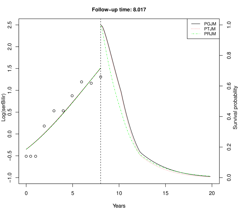
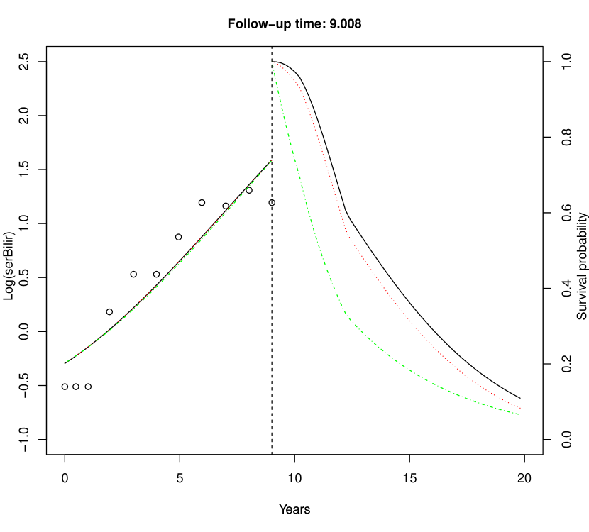
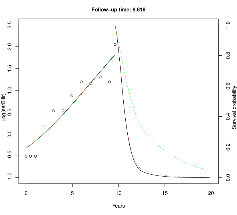
Figure 10: Dynamic prediction of survival probabilities and fitted longitudinal trajectories for subjects 21 from PBC dataset. The solid (black), , dotted (red) and dash-dotted (green) lines represent PGJM, PTJM and PRJM, respectively, in Table 4.

5 Discussion

In the paper, the regular joint model is generalised to have one more layer of correlation introduced by a bivariate functional copula, allowing us to relax the usually assumed but rarely checked assumption of conditional independence given the random effects in a regular joint model. In simulation studies, all the sub-models are correctly specified but estimated under different copulas. Moderate biases are observed in the estimations of the slope term of the longitudinal sub-model, variance components of the random effects, the association parameter and the regression parameters in the survival sub-model under the regular joint model, although the remaining parameters are relatively accurately estimated. However, the regular joint model performs significantly worse in the prediction survival probabilities with weaker discrimination capability and higher prediction error compared to the proposed model, and this is especially obvious when the correlation, described by function $\rho(t),$ is high. On the other hand, the bivariate functional Gaussian copula joint model offers more robust estimation for the correlation function than the bivariate functional $t$ copula one, although both have similarly good performance in terms of dynamic prediction of survival probabilities. Due to computational ease, selecting the bivariate functional Gaussian copula joint model seems to be a reasonable choice in practice. Compared with the multivariate Gaussian copula joint model in Zhang et al.,(2021b)[45], the proposed model has more flexibility in the correlation structure between the two sub-models as $\rho(t)$ or $\tau(t)$ is modelled by B-spline basis functions. Therefore, the dimensionality and positive definiteness of the correlation matrix in Zhang et al.(2021b)[45] is not a problem here.

The real data application on the PBC dataset indicates our model provides significantly better fitting than the regular joint model. Although there are no obvious differences in the regression parameters, the population mean function $\mu(t)$ in the regular joint model is slightly higher than the proposed model at later time points. The fitted correlation $\hat{\rho}(t)$ also indicates there is strong extra correlation between the two processes not accounted for by the random effects. The dynamic prediction of survival probabilities also shows the proposed models provide significant better predictions between $t=8$ and 11, when the correlation is strongest.

Although our model is more general than the regular joint model, conditional independence given the random effects among longitudinal measurements within a subject is still assumed. What happens under the violation of this assumption is still not clear, thus it might be interesting to investigate this issue. A more flexible functional mean function is used to capture any non-linear trends in the longitudinal trajectories, but the fixed effect regression parameters and random effects are modelled as fixed in terms of $t.$ In future work, we could also consider modelling these components functionally as in Brown et al. (2005)[4] and Yao (2007)[43]. It could also be interesting to develop a similar score test for testing conditional independence given random effects as in Jacqmin-Gadda et al. (2010)[19]. The bivariate Gaussian and $t$ copulas may also be replaced by a family of bivariate Archimedean copulas, if the range of Kendall’s $\tau$ are not required to cover $[-1,1]$ . One example is the bivariate Clayton copula, whose Kendall’s $\tau$ is between -1 and 1 except 0, as used in Emura et al. (2017)[1].

Software

R code is available at https://github.com/zhangzili0916/bivfun-copula-jointmodel-randomeffect on Github.

References

- [1] Alsefri, M., Sudell, M., García-Fiñana, M. and Kolamunnage-Dona, R. (2020) Bayesian joint modelling of longitudinal and time to event data: a methodological review. BMC Med Res Methodol 20, 94, https://doi.org/10.1186/s12874-020-00976-2
- [2] Andersen, P. K., Borgan, O., Gill, R. D. and Kieding, N. (2003) Statistical Models Based on Counting Processes. New York: Springer.
- [3] Andrinopoulou, E., Eilers, P., Takkenberg, J., and Rizopoulos, D. (2018) Improved dynamic predictions from joint models of longitudinal and survival data with time-varying effects using P-Splines. Biometrics 74, 685–693
- [4] Brown, E. R., Ibrahim, J. G. and DeGruttola, V. (2005). A flexible B-spline model for multiple longitudinal biomarkers and survival. Biometrics 61, 64-73.
- [5] Cox, D. R. (1972). Regression models and life tables (with discussion). Journal of the Royal Statistical Society, Series B 34, 187–220.
- [6] Dennis, J. E. and Schnabel, R. B. (1983). Numerical Methods for Unconstrained Optimization and Nonlinear Equations. Prentice-Hall, Englewood Cliffs, NJ.
- [7] Dutta, S., Molenberghs, G. and Chakraborty, A. (2021) Joint modelling of longitudinal response and time-to-event data using conditional distributions: a Bayesian perspective. Journal of Applied Statistics, https://doi.org/10.1080/02664763.2021.1897971
- [8] Emura, T., Nakatochi, M., Murotani, K., and Rondeau, V. (2017). A joint frailty-copula model between tumour progression and death for meta-analysis. Statistical Methods in Medical Research, 26(6), 2649–2666.
- [9] Faucett, C. L. and Thomas, D. C. (1996). Simultaneously modelling censored survival data and repeatedly measured covariates: A Gibbs sampling approach. Stat Med 15, pp. 1663–1685.
- [10] Ganjali, M. and Baghfalaki, T. (2015). A copula approach to joint modeling of longitudinal measurements and survival times using Monte Carlo expectation-maximization with application to AIDS studies. Journal of Biopharmaceutical Statistics 25, 1077-1099.
- [11] Garre, F. G., Zwinderman, A. H., Geskus, R. B. and Sijpkens, Y. W. J. (2008). A joint latent class changepoint model to improve the prediction of time to graft failure. J. R. Statist. Soc. A 171, Part 1, pp. 299–308
- [12] Guo, J., Wall, M., and Amemyia, Y. (2006). Latent class regression on latent factors. Biostatistics 7, 145–163.
- [13] Guo, X. and Carlin, B. P. (2004). Separate and Joint Modelling of Longitudinal and Event Time Data Using Standard Computer Packages, The American Statistician, 58:1, 16-24, DOI: 10.1198/0003130042854
- [14] Henderson, R., Diggle, P. and Dobson, A. (2000). Joint modelling of longitudinal measurements and event time data. Biostatistics 4, 465–480.
- [15] Hofert, M., Kojadinovic, I., Machler, M. and Yan, J. (2018). Elements of copula modelling with R. Berlin, Germany: Springer International Publishing AG. https://doi.org/10.1007/978-3-319-89635-9
- [16] Hsieh, F., Tseng, Y. K., and Wang, J. L. (2006). Joint modeling of survival and longitudinal data: likelihood approach revisited. Biometrics 62, 1037 –1043.
- [17] Ibrahim, Joseph, G., Chu, H. and Chen, L. M. (2010). Basic concepts and methods for joint models of longitudinal and survival data, Journal of Clinical Oncology, Vol. 28, pp. 2796–2801.
- [18] Jäckel, P. (2005). A note on multivariate Gauss-Hermite quadrature.
- [19] Jacqmin-Gadda, H., Proust-Lima, C., Taylor, J.M. and Commenges, D. (2010). Score test for conditional independence between longitudinal outcome and time to event given the classes in the joint latent class model. Biometrics 66, 11–19.
- [20] Li, C., Xiao, L. and Luo, S. (2021). Joint model for survival and multivariate sparse functional data with application to a study of Alzheimer’s Disease. Biometrics. 10.1111/biom.13427
- [21] Li, K. and Luo, S. (2017). Functional joint model for longitudinal and time-to-event data: an application to Alzheimer’s disease. Stat Med 36 3560–3572, DOI: 10.1002/sim.7381
- [22] Li, K. and Luo, S. (2019). Bayesian functional joint models for multivariate longitudinal and time-to-event data. Comput Stat Data Anal. 129:14–29, https://doi.org/10.1016/j.csda.2018.07.015
- [23] Lin, H., McCulloch, C. E., and Rosenheck, R. A. (2004). Latent pattern mixture models for informative intermittent missing data in longitudinal studies. Biometrics 60, 295–305.
- [24] Lin, H., Turnbull, B. W., McCulloch, C. E., and Slate, E. H. (2002). Latent class models for joint analysis of longitudinal biomarker and event process data: Application to longitudinal prostate-specific antigen readings and prostate cancer. Journal of the American Statistical Association 97, 53–65.
- [25] Malehi, A. S., Hajizadehb, E., Ahmadia, K. A., and Mansouric, P. (2015). Joint modelling of longitudinal biomarker and gap time between recurrent events: copula-based dependence. Journal of Applied Statistics, 2015 Vol. 42, No. 9, 1931–1945, http://dx.doi.org/10.1080/02664763.2015.1014889
- [26] Murtaugh, P., Dickson, E., Van Dam, G., Malincho, M., Grambsch, P., Lang worthy, A., and Gips, C. (1994). Primary biliary cirrhosis: prediction of short-term survival based on repeated patient visits. Hepatology 20, 126-134.
- [27] Nelder, J. A. and Mead, R. (1965). A simplex algorithm for function minimization. Computer Journal, 7, 308–313. 10.1093/comjnl/7.4.308.
- [28] Papageorgiou, G., Mauff, K., Tomer, A., and Rizopoulos, D. (2019). An Overview of Joint Modelling of Time-to-Event and Longitudinal Outcomes. Annual Review of Statistics and Its Application.
- [29] Proust-Lima, C., Joly, P., and Jacqmin-Gadda, H. (2009). Joint modelling of multivariate longitudinal outcomes and a time-to-event: A nonlinear latent class approach. Computational Statistics and Data Analysis 53, 1142–1154.
-
[30]
Rizopoulos, D. (2010).
JM: AnRpackage for the joint modelling of longitudinal and time-to-event data. Journal of Statistical Software 35 (9), 1-33. - [31] Rizopoulos, D. (2011). Dynamic predictions and prospective accuracy in joint models for longitudinal and time-to-event data. Biometrics 67, 819–829.
- [32] Rizopoulos, D. (2012b). Fast fitting of joint models for longitudinal and event time data using a pseudo-adaptive Gaussian quadrature rule. Comput Stat Data Anal. 56 (2012) 491–501, 11, doi:10.1016/j.csda.2011.09.007
- [33] Rizopoulos, D., Verbeke, G., and Lesaffre, E. (2008a). A two-part joint model for the analysis of survival and longitudinal binary data with excess zeros. Biometrics 64, 611–619.
- [34] Rizopoulos D., Verbeke, G., and Molenberghs, G. (2008b). Shared parameter models under random effects misspecification. Biometrika 95, 63–74.
- [35] Rondeau, V., Pignon, J. P. and Michiels, S. (2015) A joint model for dependence between clustered times to tumour progression and deaths: A meta-analysis of chemotherapy in head and neck cancer. Stat Meth Med Res 24: 711–729.
- [36] Roy, J. (2003). Modelling longitudinal data with nonignorable dropouts using a latent dropout class model. Biometrics 59, 829–836.
- [37] Suresh, K., Taylor, J. M. G., and Tsodikov, A. (2021a). A Gaussian copula approach for dynamic prediction of survival with a longitudinal biomarker. Biostatistics Volume 22, Issue 3, 504-521, doi:10.1093/biostatistics/kxz049
- [38] Suresh, K., Taylor, J. M. G., and Tsodikov, A. (2021b). A copula-based approach for dynamic prediction of survival with a binary time-dependent covariate. Biostatistics Volume 40, Issue 23, 4931-4946, https://doi.org/10.1002/sim.9102
- [39] Tsiatis, A. A. and Davidian, M. (2004). Joint modelling of longitudinal and time-to-event data: An overview. Statistica Sinica 14, 809-834.
- [40] Tsiatis, A. A., DeGruttola, V., and Wulfsohn, M. (1995). Modelling the relationship of survival to longitudinal data measured with error: Applications to survival and CD4 counts in patients with AIDS. Journal of the American Statistical Association 90, 27 – 37.
- [41] Wang, Y. and Taylor, J. M. G. (2001). Jointly modelling longitudinal and event time data with application to acquired immunodeficiency syndrome. J. Amer. Statist. Assoc. 96, 895-905.
- [42] Wulfsohn, M. S. and Tsiatis, A. A. (1997). A joint model for survival and longitudinal data measured with error. Biometrics 53, 330-339.
- [43] Yao, F. (2007). Functional Principal Component Analysis for Longitudinal and Survival Data, Statistica Sinica 17, 965–983.
- [44] Zhang, Z., Charalambous, C., and Foster, P. (2021a). Joint modelling of longitudinal measurements and survival times via a multivariate copula approach. Journal of Applied Statistics, https://doi.org/10.1080/02664763.2022.2081965
- [45] Zhang, Z., Charalambous, C., and Foster, P. (2021b). A Gaussian copula joint model for longitudinal and time-to-event data with random effects. arXiv:2112.01941