Tensor Completion via Tensor Train Based Low-Rank Quotient Geometry under a Preconditioned Metric

Abstract

Low-rank tensor completion problem is about recovering a tensor from partially observed entries. We consider this problem in the tensor train format and extend the preconditioned metric from the matrix case to the tensor case. The first-order and second-order quotient geometry of the manifold of fixed tensor train rank tensors under this metric is studied in detail. Algorithms, including Riemannian gradient descent, Riemannian conjugate gradient, and Riemannian Gauss-Newton, have been proposed for the tensor completion problem based on the quotient geometry. It has also been shown that the Riemannian Gauss-Newton method on the quotient geometry is equivalent to the Riemannian Gauss-Newton method on the embedded geometry with a specific retraction. Empirical evaluations on random instances as well as on function-related tensors show that the proposed algorithms are competitive with other existing algorithms in terms of recovery ability, convergence performance, and reconstruction quality.

Keywords. Low-rank tensor completion, tensor train decomposition, Riemannian optimization, quotient geometry, preconditioned metric

1 Introduction

Tensors are multidimensional arrays which arise in a wide range of applications, including but not limited to topic modeling [2], computer version [18], collaborative filtering [16], and signal processing [7]. Tensor completion refers to the problem of recovering the target tensor from its partial entries. It is not hard to see that, without any additional assumptions, tensor completion is an ill-posed problem. On the other hand, this problem can be solved when the target tensor possesses certain intrinsic low-dimensional structures. A notable example is low-rank tensor completion, where the target tensor is assumed to be low rank. In contrast to the matrix case, tensor has more complex rank notions up to different tensor decompositions such as CP decomposition [13], Tucker decomposition [28], tensor train (TT) decomposition [22] (also known in the computational physics community as matrix product state (MPS) [26, 31]), and hierarchical Tucker (HT) decomposition [12]. In this manuscript, we focus on the TT decomposition, a special form of the HT decomposition. Then the low-rank tensor completion problem can be formulated as follows:

$$\min_{{\cal X}\in\mathbb{R}^{n_{1}\times n_{2}\times\cdots\times n_{d}}}~{}h\left({\cal X}\right):=\frac{1}{2}\left\|{\cal P}_{\Omega}\left({\cal X}\right)-{\cal P}_{\Omega}\left({\cal T}\right)\right\|_{{\footnotesize{\mathsf{F}}}}^{2}\quad\text{s.t. }~{}\operatorname{\mathrm{rank}}_{\operatorname{TT}}\left({\cal X}\right)=\bm{r},$$ (1.1)

where ${\cal T}$ is the target tensor to be recovered, $\Omega$ is a subset of indices for the observed entries, $\operatorname{\mathrm{rank}}_{\operatorname{TT}}\left({\cal X}\right)$ is the TT rank of ${\cal X}$ which will be introduced later, and ${\cal P}_{\Omega}$ is the sampling operator defined by

$${\cal P}_{\Omega}\left({\cal X}\right)\left(i_{1},\cdots,i_{d}\right) =\begin{cases}{\cal X}\left(i_{1},\cdots,i_{d}\right),~{}&\text{if }(i_{1},\cdots,i_{d})\in\Omega,\\ 0,~{}&\text{otherwise}.\end{cases}$$

1.1 Preliminaries on Tensor Train Decomposition

Tensor train decomposition.

In the tensor train (TT) decomposition, a $d$-dimensional tensor ${\cal X}\in\mathbb{R}^{n_{1}\times n_{2}\times\cdots\times n_{d}}$ can be expressed as a product of $d$ third order tensors. More precisely, the $\left(i_{1},\cdots,i_{d}\right)$-th element of ${\cal X}$ is

$${\cal X}\left(i_{1},\cdots,i_{d}\right)=\sum_{\ell_{1}=1}^{r_{1}}\cdots\sum_{\ell_{d-1}=1}^{r_{d-1}}{\cal X}^{1}\left(1,i_{1},\ell_{1}\right){\cal X}^{2}\left(\ell_{1},i_{2},\ell_{2}\right)\cdots{\cal X}^{d}\left(\ell_{d-1},i_{d},1\right),$$

where ${\cal X}^{k}\in\mathbb{R}^{r_{k-1}\times n_{k}\times r_{k}}$ are the core tensors, $k=1,\cdots,d$, and $r_{0}=r_{d}=1$. For conciseness, we denote by ${\cal X}^{k}\left(i_{k}\right)\in\mathbb{R}^{r_{k-1}\times r_{k}}$ the $i_{k}$-th slice of ${\cal X}^{k}$ which yields the following equivalent expression

$${\cal X}\left(i_{1},\cdots,i_{d}\right)={\cal X}^{1}\left(i_{1}\right){\cal X}^{2}\left(i_{2}\right)\cdots{\cal X}^{d}\left(i_{d}\right).$$ (1.2)

In addition, for any ${\cal Z}\in\mathbb{R}^{n_{1}\times n_{2}\times n_{3}}$, the left and right unfolding operators: $L:\mathbb{R}^{n_{1}\times n_{2}\times n_{3}}\rightarrow\mathbb{R}^{n_{1}n_{2}\times n_{3}}$, $R:\mathbb{R}^{n_{1}\times n_{2}\times n_{3}}\rightarrow\mathbb{R}^{n_{1}\times n_{2}n_{3}}$ are defined as

$$L\left({\cal Z}\right)\in\mathbb{R}^{n_{1}n_{2}\times n_{3}}:L\left({\cal Z}\right)\left(i_{1}+n_{1}\left(i_{2}-1\right),i_{3}\right) ={\cal Z}\left(i_{1},i_{2},i_{3}\right),$$

$$R\left({\cal Z}\right)\in\mathbb{R}^{n_{1}\times n_{2}n_{3}}:R\left({\cal Z}\right)\left(i_{1},i_{2}+n_{2}\left(i_{3}-1\right)\right) ={\cal Z}\left(i_{1},i_{2},i_{3}\right).$$

$k$-th unfolding and interface matrices.

The $k$-th unfolding of a tensor ${\cal X}$ is a matrix of size $n_{1}\cdots n_{k}\times n_{k+1}\cdots n_{d}$, defined by

$${\cal X}^{<k>}\left(i_{1},\cdots,i_{k};i_{k+1},\cdots,i_{d}\right)={\cal X}\left(i_{1},\cdots,i_{d}\right),$$

where the semicolon represents the separation of the row and column indices: the first $k$ indices of ${\cal X}$ enumerate the rows of ${\cal X}^{<k>}$, and the last $d-k$ the columns of ${\cal X}^{<k>}$. Additionally, a tensor ${\cal X}$ with core tensors $\left\{{\cal X}^{1},\cdots,{\cal X}^{d}\right\}$ can be split into left and right parts

$${\cal X}^{\leq k}\in\mathbb{R}^{n_{1}n_{2}\cdots n_{k}\times r_{k}}:{\cal X}^{\leq k}\left(i_{1},i_{2},\cdots,i_{k};:\right) ={\cal X}^{1}\left(i_{1}\right){\cal X}^{2}\left(i_{2}\right)\cdots{\cal X}^{k}\left(i_{k}\right),$$

$${\cal X}^{\geq k}\in\mathbb{R}^{n_{k}n_{k+1}\cdots n_{d}\times r_{k-1}}:{\cal X}^{\geq k}\left(i_{k},i_{k+1},\cdots,i_{d};:\right) =\left[{\cal X}^{k}\left(i_{k}\right){\cal X}^{k+1}\left(i_{k+1}\right)\cdots{\cal X}^{d}\left(i_{d}\right)\right]^{\mathsf{T}},$$

the so-called interface matrices [27]. The following recursive relations between the interface matrices, which follow immediately from the definition, will be very useful: for $k=1,\cdots,d$,

$${\cal X}^{\leq k}=\left(\bm{I}_{n_{k}}\otimes{\cal X}^{\leq k-1}\right)L\left({\cal X}^{k}\right),$$

$${\cal X}^{\geq k}=\left({\cal X}^{\geq k+1}\otimes\bm{I}_{n_{k}}\right)R\left({\cal X}^{k}\right)^{\mathsf{T}},$$ (1.3)

where $\bm{I}_{n_{k}}$ is the identity matrix of size $n_{k}\times n_{k}$, $\otimes$ denotes the Kronecker product and ${\cal X}^{\leq 0}={\cal X}^{\geq d+1}:=1$. With these notations, the $k$-th unfolding of ${\cal X}$ can be expressed as

$${\cal X}^{<k>}={\cal X}^{\leq k}{{\cal X}^{\geq k+1}}^{\mathsf{T}}=\left(\bm{I}_{n_{k}}\otimes{\cal X}^{\leq k-1}\right)L\left({\cal X}^{k}\right){{\cal X}^{\geq k+1}}^{\mathsf{T}}={\cal X}^{\leq k}R\left({\cal X}^{k+1}\right)\left({{\cal X}^{\geq k+2}}^{\mathsf{T}}\otimes\bm{I}_{n_{k+1}}\right).$$ (1.4)

We also define the interface matrices product as follows

$$\bm{L}^{k} ={{\cal X}^{\leq k}}^{\mathsf{T}}{\cal X}^{\leq k}\in\mathbb{R}^{r_{k}\times r_{k}},$$ (1.5)

$$\bm{R}^{k} ={{\cal X}^{\geq k}}^{\mathsf{T}}{\cal X}^{\geq k}\in\mathbb{R}^{r_{k-1}\times r_{k-1}}.$$ (1.6)

TT rank.

The TT rank of a tensor ${\cal X}$ is defined as the smallest $\left(1,r_{1},\cdots,r_{d-1},1\right)$ such that ${\cal X}$ admits a TT decomposition (1.2) with core tensors of size $r_{k-1}\times n_{k}\times r_{k}$, for $k=1,\cdots,d$. The TT rank $r_{k}$ is closely related to the rank of the $k$-th unfolding of ${\cal X}$. More precisely, if a tensor can be decomposed as (1.2), it necessarily holds that $r_{k}\geq\operatorname{\mathrm{rank}}\left({\cal X}^{<k>}\right)$ [30]. Furthermore, there exists a TT decomposition with $r_{k}=\operatorname{\mathrm{rank}}\left({\cal X}^{<k>}\right)$. Consequently, $r_{k}$ is equal to the rank of ${\cal X}^{<k>}$ and

$$\operatorname{\mathrm{rank}}_{\operatorname{TT}}\left({\cal X}\right)=\bm{r}=\left(1,r_{1},\cdots,r_{d-1},1\right):=\left(1,\operatorname{\mathrm{rank}}\left({\cal X}^{<1>}\right),\cdots,\operatorname{\mathrm{rank}}\left({\cal X}^{<d-1>}\right),1\right).$$

In addition to the basics of TT decomposition, we also need the following two notions in this paper:

• The mode-$k$ product of a tensor ${\cal X}\in\mathbb{R}^{n_{1}\times n_{2}\times\cdots\times n_{d}}$ with a matrix $\bm{A}\in\mathbb{R}^{m_{k}\times n_{k}}$, denoted ${\cal X}\times_{k}\bm{A}$, yields a tensor of size $n_{1}\times\cdots\times m_{k}\times\cdots\times n_{d}$. The $\left(i_{1},\cdots,j_{k},\cdots,i_{d}\right)$-th entry of ${\cal X}\times_{k}\bm{A}$ is

  $$\left({\cal X}\times_{k}\bm{A}\right)\left(i_{1},\cdots,j_{k},\cdots,i_{d}\right)=\sum_{i_{k}=1}^{n_{k}}{\cal X}\left(i_{1},\cdots,i_{k},\cdots,i_{d}\right)\bm{A}\left(j_{k},i_{k}\right).$$

• The matricization operator for a tensor ${\cal X}\in\mathbb{R}^{n_{1}\times\cdots\times n_{d}}$ is defined as

  $${\cal M}_{k}\left({\cal X}\right)\in\mathbb{R}^{n_{k}\times\prod_{j\neq k}n_{j}}:~{}{\cal M}_{k}\left({\cal X}\right)\left(i_{k},1+\sum_{\ell=1,\ell\neq k}^{n}\left(i_{\ell}-1\right)J_{\ell}\right)={\cal X}\left(i_{1},\cdots,i_{d}\right),$$

  where $J_{\ell}=\prod_{j=1,j\neq k}^{\ell-1}n_{j}$. It can be verified that we have the following two equations related to (1.4): for $k=1,\cdots,d$,

  $${\cal M}_{3}\left({\cal X}^{k}\times_{1}{\cal X}^{\leq k-1}\times_{3}{\cal X}^{\geq k+1}\right) =\left(\left(\bm{I}_{n_{k}}\otimes{\cal X}^{\leq k-1}\right)L\left({\cal X}^{k}\right){{\cal X}^{\geq k+1}}^{\mathsf{T}}\right)^{\mathsf{T}},$$ (1.7)

  $${\cal M}_{2}\left({\cal X}^{k}\times_{1}{\cal X}^{\leq k-1}\times_{3}{\cal X}^{\geq k+1}\right) ={\cal M}_{2}\left({\cal X}^{k}\right)\left({\cal X}^{\geq k+1}\otimes{\cal X}^{\leq k-1}\right)^{\mathsf{T}}.$$

1.2 Geometric Structure

Let ${\cal M}_{\bm{r}}$ be a set of fixed tensor train rank tensors, that is

$${\cal M}_{\bm{r}}=\left\{{\cal X}\in\mathbb{R}^{n_{1}\times n_{2}\times\cdots\times n_{d}}:\operatorname{\mathrm{rank}}_{\operatorname{TT}}\left({\cal X}\right)=\bm{r}\right\}.$$ (1.8)

For ${\cal M}_{\bm{r}}$ to be non-empty, the necessary and sufficient conditions are

$$r_{k-1}\leq n_{k}r_{k},~{}r_{k}\leq n_{k}r_{k-1},~{}k=1,\cdots,d,$$

see for example [30, Section 9.3.3]. Moreover, it has been shown that the set ${\cal M}_{\bm{r}}$ forms a smooth embedded submanifold of dimension $\sum_{k=1}^{d}r_{k-1}n_{k}r_{k}-\sum_{k=1}^{d-1}r_{k}^{2}$ [14].

To introduce the quotient geometry, assume ${\cal X}$ is represented in the TT format (1.2) with core tensors $\bar{{\cal X}}:=\left\{{\cal X}^{1},\cdots,{\cal X}^{d}\right\}$. It is known that the condition $\operatorname{\mathrm{rank}}_{\operatorname{TT}}\left({\cal X}\right)=\bm{r}$ is equivalent to $\operatorname{\mathrm{rank}}\left(L\left({\cal X}^{k}\right)\right)=r_{k}$ and $\operatorname{\mathrm{rank}}\left(R\left({\cal X}^{k}\right)\right)=r_{k-1}$, $k=1,\cdots,d$ [14, 30]. We denote by $\overline{{\cal M}}_{\bm{r}}:=\mathbb{R}_{\ast}^{r_{0}\times n_{1}\times r_{1}}\times\cdots\times\mathbb{R}_{\ast}^{r_{d-1}\times n_{d}\times r_{d}}$ the set of tensors with the following rank constraint: for any ${\cal X}^{k}\in\mathbb{R}_{\ast}^{r_{k-1}\times n_{k}\times r_{k}}$, $\operatorname{\mathrm{rank}}\left(L\left({\cal X}^{k}\right)\right)=r_{k}$, and $\operatorname{\mathrm{rank}}\left(R\left({\cal X}^{k}\right)\right)=r_{k-1}$, $k=1,\cdots,d$. Let the mapping $\phi$ be

$$\phi:\overline{{\cal M}}_{\bm{r}}\rightarrow{\cal M}_{\bm{r}}:\bar{{\cal X}}\rightarrow\phi\left(\bar{{\cal X}}\right),\hbox{ such that }\phi\left(\bar{{\cal X}}\right)\left(i_{1},\cdots,i_{d}\right)={\cal X}^{1}\left(i_{1}\right){\cal X}^{2}\left(i_{2}\right)\cdots{\cal X}^{d}\left(i_{d}\right).$$

It is not hard to see that the image of $\overline{{\cal M}}_{\bm{r}}$ under $\phi$ is ${\cal M}_{\bm{r}}$. Let $\bar{{\cal X}}=\left\{{\cal X}^{1},\cdots,{\cal X}^{d}\right\}\in\overline{{\cal M}}_{\bm{r}}$ and $\bar{{\cal Y}}=\left\{{\cal Y}^{1},\cdots,{\cal Y}^{d}\right\}\in\overline{{\cal M}}_{\bm{r}}$. Then by Proposition 7 in  [29], $\phi\left(\bar{{\cal X}}\right)=\phi\left(\bar{{\cal Y}}\right)$ if and only if there exist invertible matrices $\bm{A}_{1},\cdots,\bm{A}_{d-1}$ of appropriate sizes such that

$$\bar{{\cal Y}}=\left\{{\cal X}^{1}\times_{3}\bm{A}_{1}^{\mathsf{T}},{\cal X}^{2}\times_{1}\bm{A}_{1}^{-1}\times_{3}\bm{A}_{2}^{\mathsf{T}},\cdots,{\cal X}^{d}\times_{1}\bm{A}_{d-1}^{-1}\right\}.$$ (1.9)

We denote by $\left[\bar{{\cal X}}\right]$ the set containing all points $\bar{{\cal X}}\in\overline{{\cal M}}_{\bm{r}}$ that obeys $\phi\left(\bar{{\cal X}}\right)={\cal X}$. This set is known as the equivalent class. Moreover, let ${\cal G}$ be the Lie group

$${\cal G}=\left\{\mathrm{A}=\left(\bm{A}_{1},\cdots,\bm{A}_{d-1}\right):\bm{A}_{k}\in\operatorname{GL}(r_{k}),~{}\text{for}~{}k=1,\cdots,d-1\right\},$$

where $\operatorname{GL}(r_{k})$ is the set of non-singular matrices of size $r_{k}\times r_{k}$, and define the quotient set

$$\overline{{\cal M}}_{\bm{r}}/{\cal G} =\left\{\left[\bar{{\cal X}}\right]:\bar{{\cal X}}\in\overline{{\cal M}}_{\bm{r}}\right\}.$$ (1.10)

As shown in [29], $\overline{{\cal M}}_{\bm{r}}/{\cal G}$ is a quotient manifold of dimension $\sum_{k=1}^{d}r_{k-1}n_{k}r_{k}-\sum_{k=1}^{d-1}r_{k}^{2}$.

The natural projection $\pi$ which maps the element in the total space $\overline{{\cal M}}_{\bm{r}}$ to the quotient space $\overline{{\cal M}}_{\bm{r}}/{\cal G}$ is defined as

$$\pi:\overline{{\cal M}}_{\bm{r}}\rightarrow\overline{{\cal M}}_{\bm{r}}/{\cal G}:\bar{{\cal X}}\rightarrow\pi\left(\bar{{\cal X}}\right)=\left[\bar{{\cal X}}\right].$$

Then, it is evident that there is a bijective mapping $\Phi$ from $\overline{{\cal M}}_{\bm{r}}/{\cal G}$ to ${\cal M}_{\bm{r}}$ such that $\phi=\Phi\circ\pi$. The relations between the different geometric spaces are summarized in the diagram below:

1.3 Main Contributions and Outline

For the low rank tensor completion problem in the tensor train format, several computational methods have been developed, including block coordinate descent [3], iterative hard thresholding [25], gradient-based optimization [33], Riemannian optimization [6, 27, 32]. In this paper, we study this problem based on the quotient geometry under a specific metric. The main contributions of this paper are summarized as follows:

• We extend the preconditioned metric from matrix to tensor and exploit the first order and second order geometry of the quotient manifold $\overline{{\cal M}}_{\bm{r}}/{\cal G}$ under this metric. Even though the results are extensions from the matrix case, the mathematical derivations are by no means trivial due to the complications of the tensor algebra. In particular, to compute the projection onto the horizontal space, we have to solve a system of linear equations where the coefficient matrix is symmetric and block tridiagonal. A fundamental contribution of this paper is that the positive definiteness of the coefficient matrix has been established.

• Riemannian optimization algorithms based on the quotient geometry are proposed, including Riemannian gradient descent, Riemannian conjugate gradient, and Riemannian Gauss-Newton. In particular, it has been shown that the Riemannian Gauss-Newton method on the quotient geometry is equivalent to the Riemannian Gauss-Newton method on the embedded geometry with a specific retraction. The per iteration computational complexity of the first order algorithms presented in this paper scales linearly in the dimension $d$, in the tensor size $n$ and in the sampling set size $|\Omega|$, scales polynomially in the TT rank $\bm{r}$. Overall, it is comparable with that of the Riemannian conjugate gradient method proposed in [27] based on the submanifold. Numerical experiments demonstrate that the proposed algorithms for the tensor completion problem are competitive with other state-of-the-art algorithms in terms of recovery ability, convergence performance, and reconstruction quality.

The rest of this manuscript is outlined as follows. Section $2$ investigates the first order and second order geometry of $\overline{{\cal M}}_{\bm{r}}/{\cal G}$ under the preconditioned metric. Riemannian gradient descent, Riemannian conjugate gradient, and Riemannian Gauss-Newton methods are presented in Section $3$. Empirical performance evaluations of the algorithms are given in Section $4$. In Section $5$, we conclude this paper with some future research directions.

2 Quotient Geometry under Preconditioned Metric

2.1 Preconditioned Metric and Horizontal Lift

Recall that the total space $\overline{{\cal M}}_{\bm{r}}$ is defined as $\overline{{\cal M}}_{\bm{r}}=\mathbb{R}_{\ast}^{r_{0}\times n_{1}\times r_{1}}\times\cdots\times\mathbb{R}_{\ast}^{r_{d-1}\times n_{d}\times r_{d}}$. The vertical space, denoted by ${\cal V}_{\bar{{\cal X}}}$, is the tangent space to the equivalent class $\left[\bar{{\cal X}}\right]$ at $\bar{{\cal X}}$. The expression for ${\cal V}_{\bar{{\cal X}}}$ is given in the following proposition.

Proposition 2.1.

The vertical space at $\bar{{\cal X}}$ is

$${\cal V}_{\bar{{\cal X}}}=\left\{\left\{{\cal X}^{1}\times_{3}\bm{D}_{1}^{\mathsf{T}},-{\cal X}^{2}\times_{1}\bm{D}_{1}+{\cal X}^{2}\times_{3}\bm{D}_{2}^{\mathsf{T}},\cdots,-{\cal X}^{d}\times_{1}\bm{D}_{d-1}\right\}:\bm{D}_{k}\in\mathbb{R}^{r_{k}\times r_{k}},k=1,\cdots,d-1\right\}.$$

Proof.

The proof follows from [29, Section 4.3]. ∎

Notice that the vertical space is a subspace of $T_{\bar{{\cal X}}}\overline{{\cal M}}_{\bm{r}}$. The horizontal space, denoted by ${\cal H}_{\bar{{\cal X}}}$, is any subspace of $T_{\bar{{\cal X}}}\overline{{\cal M}}_{\bm{r}}$ that is complementary to ${\cal V}_{\bar{{\cal X}}}$. For the quotient manifold $\overline{{\cal M}}_{\bm{r}}/{\cal G}$ (1.10), any element $\bar{\xi}\in T_{\bar{{\cal X}}}\overline{{\cal M}}_{\bm{r}}$ satisfying $\mathrm{D}\pi\left(\bar{{\cal X}}\right)\left[\bar{\xi}\right]=\xi_{\left[\bar{{\cal X}}\right]}$ can be seen as a representation of $\xi_{\left[\bar{{\cal X}}\right]}$ where $\xi_{\left[\bar{{\cal X}}\right]}\in T_{\left[\bar{{\cal X}}\right]}\overline{{\cal M}}_{\bm{r}}/{\cal G}$. Since the kernel of $\mathrm{D}\pi\left(\bar{{\cal X}}\right):T_{\bar{{\cal X}}}\overline{{\cal M}}_{\bm{r}}\rightarrow T_{\left[\bar{{\cal X}}\right]}\overline{{\cal M}}_{\bm{r}}/{\cal G}$ is the vertical space ${\cal V}_{\bar{{\cal X}}}$, there are infinitely many representations of $\xi_{\left[\bar{{\cal X}}\right]}$ in $T_{\bar{{\cal X}}}\overline{{\cal M}}_{\bm{r}}$. Nevertheless, one can find a unique representation of $\xi_{\left[\bar{{\cal X}}\right]}$ in horizontal space ${\cal H}_{\bar{{\cal X}}}$. The tangent vector $\bar{\xi}\in{\cal H}_{\bar{{\cal X}}}$ satisfying $\mathrm{D}\pi\left(\bar{{\cal X}}\right)\left[\bar{\xi}\right]=\xi_{\left[\bar{{\cal X}}\right]}$ is called the horizontal lift of $\xi_{\left[\bar{{\cal X}}\right]}$ at $\bar{{\cal X}}$. Throughout this paper, the horizontal lift of $\xi_{\left[\bar{{\cal X}}\right]}\in T_{\left[\bar{{\cal X}}\right]}\overline{{\cal M}}_{\bm{r}}$ at $\bar{{\cal X}}$ is denoted by $\bar{\xi}_{\bar{{\cal X}}}$.

Regarding the horizontal space, a particular one by imposing orthogonal conditions is proposed in [29]. This horizontal space has also been exploited in [8] for the development of Riemannian quotient algorithms. Moreover, given a Riemannian metric $\bar{g}\left(\cdot,\cdot\right)$, one can construct the horizontal space ${\cal H}_{\bar{{\cal X}}}$ which is orthogonal complementary to the vertical space ${\cal V}_{\bar{{\cal X}}}$:

$${\cal H}_{\bar{{\cal X}}}=\left\{\bar{\xi}\in T_{\bar{{\cal X}}}\overline{{\cal M}}_{\bm{r}}:\bar{g}_{\bar{{\cal X}}}\left(\bar{\xi},\bar{\eta}\right)=0,~{}\text{for all}~{}\bar{\eta}\in{\cal V}_{\bar{{\cal X}}}\right\}.$$ (2.1)

In this manuscript, we consider a preconditioned metric which is extended from the matrix case [9, 17, 20, 21, 34]. Let $\mathbb{R}_{\ast}^{n_{1}\times r}\times\mathbb{R}_{\ast}^{n_{2}\times r}$ be the space of matrices with full column rank $r$. Given $\bar{x}:=\left\{\bm{G},\bm{H}\right\}\in\mathbb{R}_{\ast}^{n_{1}\times r}\times\mathbb{R}_{\ast}^{n_{2}\times r}$, the preconditioned metric on the tangent space of $\mathbb{R}_{\ast}^{n_{1}\times r}\times\mathbb{R}_{\ast}^{n_{2}\times r}$ at $\bar{x}$ is defined as

$$\bar{g}_{\bar{x}}\left(\bar{\xi},\bar{\eta}\right)=\operatorname{trace}\left({\xi^{1}}^{\mathsf{T}}\eta^{1}\left(\bm{H}^{\mathsf{T}}\bm{H}\right)\right)+\operatorname{trace}\left({\xi^{2}}^{\mathsf{T}}\eta^{2}\left(\bm{G}^{\mathsf{T}}\bm{G}\right)\right),$$ (2.2)

where $\bar{\xi}=\left\{\xi^{1},\xi^{2}\right\}$ and $\bar{\eta}=\left\{\eta^{1},\eta^{2}\right\}\in T_{\bar{x}}\mathbb{R}_{\ast}^{n_{1}\times r}\times\mathbb{R}_{\ast}^{n_{2}\times r}$. Under this metric, the Riemannian gradient of a function $\bar{f}$ at $\bar{x}$ is given by

$$\operatorname{grad}\bar{f}(\bar{x})=\left(\nabla_{\bm{G}}\bar{f}(\bar{x})\left(\bm{H}^{\mathsf{T}}\bm{H}\right)^{-1},\nabla_{\bm{H}}\bar{f}(\bar{x})\left(\bm{G}^{\mathsf{T}}\bm{G}\right)^{-1}\right),$$ (2.3)

where $\nabla_{\bm{G}}\bar{f}(\bar{x})$ and $\nabla_{\bm{H}}\bar{f}(\bar{x})$ are the Euclidean partial derivatives of $\bar{f}$. Equivalently, we rewrite (2.3) in a vectorization form as

$$\operatorname{vec}\left(\operatorname{grad}\bar{f}(\bar{x})\right) =\underbrace{\begin{bmatrix}\left(\bm{H}^{\mathsf{T}}\bm{H}\right)^{-1}\otimes\bm{I}_{n_{1}}&\bm{0}\\ \bm{0}&\left(\bm{G}^{\mathsf{T}}\bm{G}\right)^{-1}\otimes\bm{I}_{n_{2}}\end{bmatrix}}_{=:\bm{J}^{-1}}\operatorname{vec}\left(\left(\nabla_{\bm{G}}\bar{f}(\bar{x}),\nabla_{\bm{H}}\bar{f}(\bar{x})\right)\right).$$

Thus, the Riemannian gradient descent direction (2.3) can be viewed as an approximation of the Newton direction. The metric in (2.2) is known as the preconditioned metric on $\mathbb{R}_{\ast}^{n_{1}\times r}\times\mathbb{R}_{\ast}^{n_{2}\times r}$.

Note that it is not evident to extend the preconditioned metric from the form presented in (2.2) because there are tensor factors in the TT format. However, the following equivalent expression of (2.2) provides a more convenient form for the extension:

$$\bar{g}_{\bar{x}}\left(\bar{\xi},\bar{\eta}\right)=\left\langle\xi^{1}\bm{H}^{\mathsf{T}},\eta^{1}\bm{H}^{\mathsf{T}}\right\rangle+\left\langle\bm{G}{\xi^{2}}^{\mathsf{T}},\bm{G}{\eta^{2}}^{\mathsf{T}}\right\rangle.$$

Basically, the precondition metric is given by replacing each factors in $\left\langle\bm{G}\bm{H}^{\mathsf{T}},\bm{G}\bm{H}^{\mathsf{T}}\right\rangle$ by the corresponding tangent vectors in the same mode. This observation leads to the following generalization in the tensor case.

Definition 2.1.

Given $\bar{{\cal X}}=\left\{{\cal X}^{1},\cdots,{\cal X}^{d}\right\}\in\overline{{\cal M}}_{\bm{r}}$, the preconditioned metric $\bar{g}_{\bar{{\cal X}}}:T_{\bar{{\cal X}}}\overline{{\cal M}}_{\bm{r}}\times T_{\bar{{\cal X}}}\overline{{\cal M}}_{\bm{r}}$ is defined as follows:

$$\bar{g}_{\bar{{\cal X}}}\left(\bar{\xi},\bar{\eta}\right) =\sum_{k=1}^{d}\left\langle\phi\left(\left\{{\cal X}^{1},\cdots,{\cal X}^{k-1},\xi^{k},{\cal X}^{k+1},\cdots,{\cal X}^{d}\right\}\right),\phi\left(\left\{{\cal X}^{1},\cdots,{\cal X}^{k-1},\eta^{k},{\cal X}^{k+1},\cdots,{\cal X}^{d}\right\}\right)\right\rangle,$$ (2.4)

where $\bar{\xi}:=\left\{\xi^{k}\right\}_{k=1}^{d},\bar{\eta}:=\left\{\eta^{k}\right\}_{k=1}^{d}\in T_{\bar{{\cal X}}}\overline{{\cal M}}_{\bm{r}}$.

Lemma 2.1.

The preconditioned metric defined in (2.4) has the following equivalent expression:

$$\bar{g}_{\bar{{\cal X}}}\left(\bar{\xi},\bar{\eta}\right)=\sum_{k=1}^{d}\operatorname{trace}\left({\cal M}_{2}\left(\xi^{k}\right)^{\mathsf{T}}{\cal M}_{2}\left(\eta^{k}\right)\left({\bm{H}^{k}}^{\mathsf{T}}\bm{H}^{k}\right)\right),$$

which coincides with that in (2.2). Here $\bm{H}^{k}={\cal X}^{\geq k+1}\otimes{\cal X}^{\leq k-1}$, for $k=1,\cdots,d$.

Proof.

The application of (1.4) yields that

$$\bar{g}_{\bar{{\cal X}}}\left(\bar{\xi},\bar{\eta}\right) =\sum_{k=1}^{d}\left\langle\phi\left(\left\{{\cal X}^{1},\cdots,{\cal X}^{k-1},\xi^{k},{\cal X}^{k+1},\cdots,{\cal X}^{d}\right\}\right),\phi\left(\left\{{\cal X}^{1},\cdots,{\cal X}^{k-1},\eta^{k},{\cal X}^{k+1},\cdots,{\cal X}^{d}\right\}\right)\right\rangle,$$

$$=\sum_{k=1}^{d}\left\langle\left(\bm{I}_{n_{k}}\otimes{\cal X}^{\leq k-1}\right)L\left(\xi^{k}\right){{\cal X}^{\geq k+1}}^{\mathsf{T}},\left(\bm{I}_{n_{k}}\otimes{\cal X}^{\leq k-1}\right)L\left(\eta^{k}\right){{\cal X}^{\geq k+1}}^{\mathsf{T}}\right\rangle$$

$$=\sum_{k=1}^{d}\left\langle\xi^{k}\times_{1}{\cal X}^{\leq k-1}\times_{3}{\cal X}^{\geq k+1},\eta^{k}\times_{1}{\cal X}^{\leq k-1}\times_{3}{\cal X}^{\geq k+1}\right\rangle$$

$$=\sum_{k=1}^{d}\left\langle{\cal M}_{2}\left(\xi^{k}\right){\bm{H}^{k}}^{\mathsf{T}},{\cal M}_{2}\left(\eta^{k}\right){\bm{H}^{k}}^{\mathsf{T}}\right\rangle$$

$$=\sum_{k=1}^{d}\operatorname{trace}\left({\cal M}_{2}\left(\xi^{k}\right)^{\mathsf{T}}{\cal M}_{2}\left(\eta^{k}\right)\left({\bm{H}^{k}}^{\mathsf{T}}\bm{H}^{k}\right)\right),$$

where the second and third equations follow from (1.7). ∎

Proposition 2.2.

Under the preconditioned metric $\bar{g}_{\bar{{\cal X}}}$ defined in (2.4), the horizontal space at $\bar{{\cal X}}$ is

$${\cal H}_{\bar{{\cal X}}} =\bigg{\{}\bar{\xi}\in T_{\bar{{\cal X}}}\overline{{\cal M}}_{\bm{r}}:L\left({\cal X}^{k}\right)^{\mathsf{T}}\left(\bm{I}_{n_{k}}\otimes\bm{L}^{k-1}\right)L\left(\xi^{k}\right)\bm{R}^{k+1}$$

$$\qquad\qquad\qquad\qquad=\bm{L}^{k}R\left(\xi^{k+1}\right)\left(\bm{R}^{k+2}\otimes\bm{I}_{n_{k+1}}\right)R\left({\cal X}^{k+1}\right)^{\mathsf{T}},k=1,\cdots,d-1\bigg{\}}.$$

Proof.

By the definition of the horizontal space in (2.1), for a tangent vector $\bar{\xi}\in{\cal H}_{\bar{{\cal X}}}$, we must have $\bar{g}_{\bar{{\cal X}}}\left(\bar{\xi},\bar{\eta}\right)=0$ for all $\bar{\eta}\in{\cal V}_{\bar{{\cal X}}}$. With the application of Proposition 2.1, the equation $\bar{g}_{\bar{{\cal X}}}\left(\bar{\xi},\bar{\eta}\right)=0$ reduces to

$$0 =\sum_{k=1}^{d}\left\langle\phi\left(\left\{{\cal X}^{1},\cdots,\xi^{k},\cdots,{\cal X}^{d}\right\}\right),\phi\left(\left\{{\cal X}^{1},\cdots,\eta^{k},\cdots,{\cal X}^{d}\right\}\right)\right\rangle$$

$$=\left\langle\phi\left(\left\{\xi^{1},\cdots,{\cal X}^{d}\right\}\right),\phi\left(\left\{{\cal X}^{1}\times_{3}\bm{D}_{1}^{\mathsf{T}},\cdots,{\cal X}^{d}\right\}\right)\right\rangle+\left\langle\phi\left(\left\{{\cal X}^{1},\cdots,\xi^{d}\right\}\right),\phi\left(\left\{{\cal X}^{1},\cdots,-{\cal X}^{d}\times_{1}\bm{D}_{d-1}\right\}\right)\right\rangle$$

$$\quad+\sum_{k=2}^{d-1}\left\langle\phi\left(\left\{{\cal X}^{1},\cdots,\xi^{k},\cdots,{\cal X}^{d}\right\}\right),\phi\left(\left\{{\cal X}^{1},\cdots,-{\cal X}^{k}\times_{1}\bm{D}_{k-1}+{\cal X}^{k}\times_{3}\bm{D}_{k}^{\mathsf{T}},\cdots,{\cal X}^{d}\right\}\right)\right\rangle$$

$$=\sum_{k=1}^{d-1}\left\langle\phi\left(\left\{{\cal X}^{1},\cdots,\xi^{k},\cdots,{\cal X}^{d}\right\}\right)-\phi\left(\left\{{\cal X}^{1},\cdots,\xi^{k+1},\cdots,{\cal X}^{d}\right\}\right),\phi\left(\left\{{\cal X}^{1},\cdots,{\cal X}^{k}\times_{3}\bm{D}_{k}^{\mathsf{T}},\cdots,{\cal X}^{d}\right\}\right)\right\rangle$$

$$=\sum_{k=1}^{d-1}\left\langle\left(\bm{I}_{n_{k}}\otimes{\cal X}^{\leq k-1}\right)L\left(\xi^{k}\right){{\cal X}^{\geq k+1}}^{\mathsf{T}}-{\cal X}^{\leq k}R\left(\xi^{k+1}\right)\left({{\cal X}^{\geq k+2}}^{\mathsf{T}}\otimes\bm{I}_{n_{k+1}}\right),{\cal X}^{\leq k}\bm{D}_{k}{{\cal X}^{\geq k+1}}^{\mathsf{T}}\right\rangle$$

$$=\sum_{k=1}^{d-1}\left\langle{{\cal X}^{\leq k}}^{\mathsf{T}}\left(\left(\bm{I}_{n_{k}}\otimes{\cal X}^{\leq k-1}\right)L\left(\xi^{k}\right){{\cal X}^{\geq k+1}}^{\mathsf{T}}-{\cal X}^{\leq k}R\left(\xi^{k+1}\right)\left({{\cal X}^{\geq k+2}}^{\mathsf{T}}\otimes\bm{I}_{n_{k+1}}\right)\right){\cal X}^{\geq k+1},\bm{D}_{k}\right\rangle$$

$$=\sum_{k=1}^{d-1}\left\langle L\left({\cal X}^{k}\right)^{\mathsf{T}}\left(\bm{I}_{n_{k}}\otimes\bm{L}^{k-1}\right)L\left(\xi^{k}\right)\bm{R}^{k+1}-\bm{L}^{k}R\left(\xi^{k+1}\right)\left(\bm{R}^{k+2}\otimes\bm{I}_{n_{k+1}}\right)R\left({\cal X}^{k+1}\right)^{\mathsf{T}},\bm{D}_{k}\right\rangle$$

where the fourth equation is due to (1.4) and the last line follows from (1.1) and (1.5). Since $\bm{D}_{k}\in\mathbb{R}^{r_{k}\times r_{k}}$ is an arbitrary matrix, one can conclude that for $k=1,\cdots,d-1$,

$$L\left({\cal X}^{k}\right)^{\mathsf{T}}\left(\bm{I}_{n_{k}}\otimes\bm{L}^{k-1}\right)L\left(\xi^{k}\right)\bm{R}^{k+1}=\bm{L}^{k}R\left(\xi^{k+1}\right)\left(\bm{R}^{k+2}\otimes\bm{I}_{n_{k+1}}\right)R\left({\cal X}^{k+1}\right)^{\mathsf{T}},$$ (2.5)

which completes the proof. ∎

The projections of any $\bar{\xi}=\left\{\xi^{1},\cdots,\xi^{d}\right\}\in T_{\bar{{\cal X}}}\overline{{\cal M}}_{\bm{r}}$ onto the vertical and horizontal spaces, denoted ${\cal P}_{\bar{{\cal X}}}^{{\cal V}}\left(\bar{\xi}\right)$ and ${\cal P}_{\bar{{\cal X}}}^{{\cal H}}\left(\bar{\xi}\right)$, are given by the following lemma.

Lemma 2.2.

Under the preconditioned metric $\bar{g}_{\bar{{\cal X}}}$ defined in (2.4), the projections onto the vertical and horizontal spaces are given by

$${\cal P}_{\bar{{\cal X}}}^{{\cal V}}\left(\bar{\xi}\right) =\left({\cal X}^{1}\times_{3}\bm{D}_{1}^{\mathsf{T}},-{\cal X}^{2}\times_{1}\bm{D}_{1}+{\cal X}^{2}\times_{3}\bm{D}_{2}^{\mathsf{T}},\cdots,-{\cal X}^{d}\times_{1}\bm{D}_{d-1}\right),$$

$${\cal P}_{\bar{{\cal X}}}^{{\cal H}}\left(\bar{\xi}\right) =\left(\xi^{1}-{\cal X}^{1}\times_{3}\bm{D}_{1}^{\mathsf{T}},\xi^{2}+{\cal X}^{2}\times_{1}\bm{D}_{1}-{\cal X}^{2}\times_{3}\bm{D}_{2}^{\mathsf{T}},\cdots,\xi^{d}+{\cal X}^{d}\times_{1}\bm{D}_{d-1}\right).$$ (2.6)

where $\bm{D}_{k}\in\mathbb{R}^{r_{k}\times r_{k}}$ are uniquely determined by the following system of linear equations

$$\begin{bmatrix}\bm{A}_{1}&\bm{B}_{1}\\ \bm{B}_{1}^{\mathsf{T}}&\bm{A}_{2}&\bm{B}_{2}\\ &\ddots&\ddots&\ddots\\ &&\bm{B}_{d-2}^{\mathsf{T}}&\bm{A}_{d-1}\end{bmatrix}\begin{bmatrix}\operatorname{vec}(\bm{D}_{1})\\ \operatorname{vec}(\bm{D}_{2})\\ \vdots\\ \operatorname{vec}(\bm{D}_{d-1})\end{bmatrix}=\begin{bmatrix}\bm{b}_{1}\\ \bm{b}_{2}\\ \vdots\\ \bm{b}_{d-1}\end{bmatrix}.$$ (2.7)

Here, the matrices $\bm{A}_{k}$,$\bm{B}_{k}$ and $\bm{b}_{k}$ are

$$\bm{A}_{k} =\bm{R}^{k+1}\otimes\bm{L}^{k},$$

$$\bm{B}_{k} =-\frac{1}{2}\left(R\left({\cal X}^{k+1}\right)\otimes\bm{L}^{k}\right)\left(\bm{R}^{k+2}\otimes L\left({\cal X}^{k+1}\right)\right),$$

$$\bm{b}_{k} =\frac{1}{2}\left(\left(\bm{R}^{k+1}\otimes L\left({\cal X}^{k}\right)^{\mathsf{T}}\right)\operatorname{vec}\left(\xi^{k}\times_{1}\bm{L}^{k-1}\right)-\left(R\left({\cal X}^{k+1}\right)\otimes\bm{L}^{k}\right)\operatorname{vec}\left(\xi^{k+1}\times_{3}\bm{R}^{k+2}\right)\right).$$

Proof.

Since ${\cal P}_{\bar{{\cal X}}}^{{\cal H}}\left(\bar{\xi}\right)\in{\cal H}_{\bar{{\cal X}}}$, the elements of ${\cal P}_{\bar{{\cal X}}}^{{\cal H}}\left(\bar{\xi}\right)$ must satisfy the equation (2.5). Substituting the $k$-th core tensor of ${\cal P}_{\bar{{\cal X}}}^{{\cal H}}\left(\bar{\xi}\right)$ into (2.5) yields that

$$\bm{L}^{k}\bm{D}_{k}\bm{R}^{k+1} =\frac{1}{2}L\left({\cal X}^{k}\right)^{\mathsf{T}}\left(\bm{I}_{n_{k}}\otimes\bm{L}^{k-1}\right)L\left(\xi^{k}+{\cal X}^{k}\times_{1}\bm{D}_{k-1}\right)\bm{R}^{k+1}$$

$$\quad-\frac{1}{2}\bm{L}^{k}R\left(\xi^{k+1}-{\cal X}^{k+1}\times_{3}\bm{D}_{k+1}^{\mathsf{T}}\right)\left(\bm{R}^{k+2}\otimes\bm{I}_{n_{k+1}}\right)R\left({\cal X}^{k+1}\right)^{\mathsf{T}}.$$

Vectorizing both sides of this equation gives that

$$\left(\bm{R}^{k+1}\otimes\bm{L}^{k}\right)\operatorname{vec}\left(\bm{D}_{k}\right) =\frac{1}{2}\left(\bm{R}^{k+1}\otimes L\left({\cal X}^{k}\right)^{\mathsf{T}}\right)\operatorname{vec}\left(\left(\bm{I}_{n_{k}}\otimes\bm{L}^{k-1}\right)L\left(\xi^{k}+{\cal X}^{k}\times_{1}\bm{D}_{k-1}\right)\right)$$

$$\quad-\frac{1}{2}\left(R\left({\cal X}^{k+1}\right)\otimes\bm{L}^{k}\right)\operatorname{vec}\left(R\left(\xi^{k+1}-{\cal X}^{k+1}\times_{3}\bm{D}_{k+1}^{\mathsf{T}}\right)\left(\bm{R}^{k+2}\otimes\bm{I}_{n_{k+1}}\right)\right)$$

$$=\frac{1}{2}\left(\bm{R}^{k+1}\otimes L\left({\cal X}^{k}\right)^{\mathsf{T}}\right)\operatorname{vec}\left(\xi^{k}\times_{1}\bm{L}^{k-1}+{\cal X}^{k}\times_{1}\left(\bm{L}^{k-1}\bm{D}_{k-1}\right)\right)$$

$$\quad-\frac{1}{2}\left(R\left({\cal X}^{k+1}\right)\otimes\bm{L}^{k}\right)\operatorname{vec}\left(\xi^{k+1}\times_{3}\bm{R}^{k+2}-{\cal X}^{k+1}\times_{3}\left(\bm{R}^{k+2}\bm{D}_{k+1}^{\mathsf{T}}\right)\right)$$

$$=\frac{1}{2}\left(\bm{R}^{k+1}\otimes L\left({\cal X}^{k}\right)^{\mathsf{T}}\right)\left(R\left({\cal X}^{k}\right)^{\mathsf{T}}\otimes\bm{L}^{k-1}\right)\operatorname{vec}\left(\bm{D}_{k-1}\right)$$

$$\quad+\frac{1}{2}\left(R\left({\cal X}^{k+1}\right)\otimes\bm{L}^{k}\right)\left(\bm{R}^{k+2}\otimes L\left({\cal X}^{k+1}\right)\right)\operatorname{vec}\left(\bm{D}_{k+1}\right)$$

$$\quad+\frac{1}{2}\left(\bm{R}^{k+1}\otimes L\left({\cal X}^{k}\right)^{\mathsf{T}}\right)\operatorname{vec}\left(\xi^{k}\times_{1}\bm{L}^{k-1}\right)$$

$$\quad-\frac{1}{2}\left(R\left({\cal X}^{k+1}\right)\otimes\bm{L}^{k}\right)\operatorname{vec}\left(\xi^{k+1}\times_{3}\bm{R}^{k+2}\right),$$

where the second equation is due to (1.7). Thus one can obtain $d-1$ equations for $k=1,\cdots,d-1$. Stacking them together yields the system of linear equations (2.7). The existence and uniqueness of projection implies the invertibility of the coefficient matrix in (2.7). As a result, $\bm{D}_{k}\in\mathbb{R}^{r_{k}\times r_{k}}$ can be uniquely obtained by solving (2.7). ∎

Moreover, it can be shown that the coefficient matrix in (2.7) is positive definite.

Lemma 2.3.

The symmetric block tridiagonal matrix in (2.7) is positive definite.

Proof.

Since the symmetric block tridiagonal matrix in (2.7) is invertible, we only need to verify the positive semidefiniteness of this matrix. For any $\bm{x}=\left[\bm{x}_{1}^{\mathsf{T}},\cdots,\bm{x}_{d-1}^{\mathsf{T}}\right]^{\mathsf{T}}\in\mathbb{R}^{\sum_{k=1}^{d-1}r_{k}^{2}}$ with $\bm{x}_{k}\in\mathbb{R}^{r_{k}^{2}}$, $k=1,\cdots,d-1$, we have

$$\bm{x}^{\mathsf{T}}\underbrace{\begin{bmatrix}\bm{A}_{1}&\bm{B}_{1}\\ \bm{B}_{1}^{\mathsf{T}}&\bm{A}_{2}&\bm{B}_{2}\\ &\ddots&\ddots&\ddots\\ &&\bm{B}_{d-2}^{\mathsf{T}}&\bm{A}_{d-1}\end{bmatrix}}_{:=\bm{M}}\bm{x} =\begin{bmatrix}\bm{x}_{1}^{\mathsf{T}}&\bm{x}_{2}^{\mathsf{T}}\end{bmatrix}\begin{bmatrix}\bm{A}_{1}&\bm{B}_{1}\\ \bm{B}_{1}^{\mathsf{T}}&\frac{1}{2}\bm{A}_{2}\end{bmatrix}\begin{bmatrix}\bm{x}_{1}\\ \bm{x}_{2}\end{bmatrix}+\begin{bmatrix}\bm{x}_{2}^{\mathsf{T}}&\bm{x}_{3}^{\mathsf{T}}\end{bmatrix}\begin{bmatrix}\frac{1}{2}\bm{A}_{2}&\bm{B}_{2}\\ \bm{B}_{2}^{\mathsf{T}}&\frac{1}{2}\bm{A}_{3}\end{bmatrix}\begin{bmatrix}\bm{x}_{2}\\ \bm{x}_{3}\end{bmatrix}$$

$$\quad+\cdots+\begin{bmatrix}\bm{x}_{d-2}^{\mathsf{T}}&\bm{x}_{d-1}^{\mathsf{T}}\end{bmatrix}\begin{bmatrix}\frac{1}{2}\bm{A}_{d-2}&\bm{B}_{d-2}\\ \bm{B}_{d-2}^{\mathsf{T}}&\bm{A}_{d-1}\end{bmatrix}\begin{bmatrix}\bm{x}_{d-2}\\ \bm{x}_{d-1}\end{bmatrix}$$

$$\geq\sum_{k=1}^{d-2}\begin{bmatrix}\bm{x}_{k}^{\mathsf{T}}&\bm{x}_{k+1}^{\mathsf{T}}\end{bmatrix}\underbrace{\begin{bmatrix}\frac{1}{2}\bm{A}_{k}&\bm{B}_{k}\\ \bm{B}_{k}^{\mathsf{T}}&\frac{1}{2}\bm{A}_{k+1}\end{bmatrix}}_{:=\bm{M}_{k}}\begin{bmatrix}\bm{x}_{k}\\ \bm{x}_{k+1}\end{bmatrix}.$$

We will next show that the matrices $\bm{M}_{k}$ are positive semidefinite which naturally yields the positive semidefiniteness of the matrix $\bm{M}$.

First, it is not hard to see that $\bm{A}_{k}$ is invertible and positive definite. Thus, by Proposition 2.2 in [10], a sufficient and necessary condition for $\bm{M}_{k}\succeq 0$ is $\frac{1}{2}\bm{A}_{k+1}-\bm{B}_{k}^{\mathsf{T}}\left(\frac{1}{2}\bm{A}_{k}\right)^{-1}\bm{B}_{k}\succeq 0$. The application of (1.1) yields that

$$\bm{L}^{k+1} =L\left({\cal X}^{k+1}\right)^{\mathsf{T}}\left(\bm{I}_{n_{k+1}}\otimes\bm{L}^{k}\right)L\left({\cal X}^{k+1}\right),$$

$$\bm{R}^{k+1} =R\left({\cal X}^{k+1}\right)\left(\bm{R}^{k+2}\otimes\bm{I}_{n_{k+1}}\right)R\left({\cal X}^{k+1}\right)^{\mathsf{T}}.$$

It can be seen that

$$\bm{A}_{k+1}-4\cdot\bm{B}_{k}^{\mathsf{T}}\bm{A}_{k}^{-1}\bm{B}_{k}$$

$$\quad=\bm{R}^{k+2}\otimes\bm{L}^{k+1}-\left(\bm{R}^{k+2}\otimes L\left({\cal X}^{k+1}\right)^{\mathsf{T}}\right)\left(R\left({\cal X}^{k+1}\right)^{\mathsf{T}}{\bm{R}^{k+1}}^{-1}R\left({\cal X}^{k+1}\right)\otimes\bm{L}^{k}\right)\left(\bm{R}^{k+2}\otimes L\left({\cal X}^{k+1}\right)\right)$$

$$\quad=\left(\bm{R}^{k+2}\otimes L\left({\cal X}^{k+1}\right)^{\mathsf{T}}\right)\left(\left({\bm{R}^{k+2}}^{-1}\otimes\bm{I}_{n_{k+1}}-R\left({\cal X}^{k+1}\right)^{\mathsf{T}}{\bm{R}^{k+1}}^{-1}R\left({\cal X}^{k+1}\right)\right)\otimes\bm{L}^{k}\right)\left(\bm{R}^{k+2}\otimes L\left({\cal X}^{k+1}\right)\right).$$

Let $\bm{R}^{k+2}=\bm{U}\bm{\Sigma}\bm{U}^{\mathsf{T}}$ be the eigenvalue decomposition of $\bm{R}^{k+2}$ and $R\left({\cal X}^{k+1}\right)\left(\bm{U}\bm{\Sigma}^{1/2}\otimes\bm{I}_{n_{k+1}}\right)=\bm{X}\bm{\Lambda}\bm{Y}^{\mathsf{T}}$ be the singular value decomposition of $R\left({\cal X}^{k+1}\right)\left(\bm{U}\bm{\Sigma}^{1/2}\otimes\bm{I}_{n_{k+1}}\right)$. One has $\bm{R}^{k+1}=\bm{X}\bm{\Lambda}^{2}\bm{X}^{\mathsf{T}}$ which is the eigenvalue decomposition of $\bm{R}^{k+1}$. It follows that

$$R\left({\cal X}^{k+1}\right)^{\mathsf{T}}{\bm{R}^{k+1}}^{-1}R\left({\cal X}^{k+1}\right)$$

$$~{}=R\left({\cal X}^{k+1}\right)^{\mathsf{T}}\bm{X}\bm{\Lambda}^{-2}\bm{X}^{\mathsf{T}}R\left({\cal X}^{k+1}\right)$$

$$~{}=\left(\bm{U}\bm{\Sigma}^{-1/2}\bm{\Sigma}^{1/2}\bm{U}^{\mathsf{T}}\otimes\bm{I}_{n_{k}}\right)R\left({\cal X}^{k+1}\right)^{\mathsf{T}}\bm{X}\bm{\Lambda}^{-2}\bm{X}^{\mathsf{T}}R\left({\cal X}^{k+1}\right)\left(\bm{U}\bm{\Sigma}^{1/2}\bm{\Sigma}^{-1/2}\bm{U}^{\mathsf{T}}\otimes\bm{I}_{n_{k+1}}\right)$$

$$~{}=\left(\bm{U}\bm{\Sigma}^{-1/2}\otimes\bm{I}_{n_{k+1}}\right)\left(\bm{Y}\bm{\Lambda}\bm{X}^{\mathsf{T}}\bm{X}\bm{\Lambda}^{-2}\bm{X}^{\mathsf{T}}\bm{X}\bm{\Lambda}\bm{Y}^{\mathsf{T}}\right)\left(\bm{\Sigma}^{-1/2}\bm{U}^{\mathsf{T}}\otimes\bm{I}_{n_{k+1}}\right)$$

$$~{}=\left(\bm{U}\bm{\Sigma}^{-1/2}\otimes\bm{I}_{n_{k+1}}\right)\bm{Y}\bm{Y}^{\mathsf{T}}\left(\bm{\Sigma}^{-1/2}\bm{U}^{\mathsf{T}}\otimes\bm{I}_{n_{k+1}}\right).$$

Then, one can obtain

$${\bm{R}^{k+2}}^{-1}\otimes\bm{I}_{n_{k+1}}-R\left({\cal X}^{k+1}\right)^{\mathsf{T}}{\bm{R}^{k+1}}^{-1}R\left({\cal X}^{k+1}\right)$$

$$\quad=\bm{U}\bm{\Sigma}^{-1}\bm{U}^{\mathsf{T}}\otimes\bm{I}_{n_{k+1}}-\left(\bm{U}\bm{\Sigma}^{-1/2}\otimes\bm{I}_{n_{k+1}}\right)\bm{Y}\bm{Y}^{\mathsf{T}}\left(\bm{\Sigma}^{-1/2}\bm{U}^{\mathsf{T}}\otimes\bm{I}_{n_{k+1}}\right)$$

$$\quad=\left(\bm{U}\bm{\Sigma}^{-1/2}\otimes\bm{I}_{n_{k+1}}\right)\left(\bm{I}_{n_{k+1}r_{k+1}}-\bm{Y}\bm{Y}^{\mathsf{T}}\right)\left(\bm{\Sigma}^{-1/2}\bm{U}^{\mathsf{T}}\otimes\bm{I}_{n_{k+1}}\right)\succeq 0.$$

Consequently, $\bm{M}_{k}\succeq 0$ for $k=1,\cdots,d-2$ which indicates the positive definiteness of the matrix $\bm{M}$. ∎

2.2 Riemannian Metric

In this section we verify that the preconditioned metric defined on $T_{\bar{{\cal X}}}\overline{{\cal M}}_{\bm{r}}$, see (2.4), indeed induces a Riemannian metric on $T_{\left[\bar{{\cal X}}\right]}\overline{{\cal M}}_{\bm{r}}/{\cal G}$. To this end, we first establish the relation between the horizontal lifts of $\xi_{\left[\bar{{\cal X}}\right]}\in T_{\left[\bar{{\cal X}}\right]}\overline{{\cal M}}_{\bm{r}}/{\cal G}$ at different elements in $\left[\bar{{\cal X}}\right]$.

Lemma 2.4.

Given $\xi_{\left[\bar{{\cal X}}\right]}\in T_{\left[\bar{{\cal X}}\right]}\overline{{\cal M}}_{\bm{r}}/{\cal G}$, suppose that the horizontal lift of $\xi_{\left[\bar{{\cal X}}\right]}$ at $\bar{{\cal X}}$ is $\bar{\xi}_{\bar{{\cal X}}}$. Then for any $\bar{{\cal Y}}\in\left[\bar{{\cal X}}\right]$, the horizontal lift of $\xi_{\left[\bar{{\cal X}}\right]}$ at $\bar{{\cal Y}}$ satisfies

$$\bar{\xi}_{\bar{{\cal Y}}}=\theta_{A}\left(\bar{\xi}_{\bar{{\cal X}}}\right):=\left\{\xi^{1}\times_{3}\bm{A}_{1}^{\mathsf{T}},\xi^{2}\times_{1}\bm{A}_{1}^{-1}\times_{3}\bm{A}_{2}^{\mathsf{T}},\cdots,\xi^{d}\times_{1}\bm{A}_{d-1}^{-1}\right\},$$

where $\bar{\xi}_{\bar{{\cal X}}}=\left\{\xi^{1},\cdots,\xi^{d}\right\}$ and $\bm{A}_{1},\cdots,\bm{A}_{d-1}$ are invertible matrices such that (1.9) holds.

Proof.

By the chain rule,

$$\xi_{\left[\bar{{\cal X}}\right]} =\mathrm{D}\pi\left(\bar{{\cal X}}\right)\left[\bar{\xi}_{\bar{{\cal X}}}\right]=\mathrm{D}\pi\left(\theta_{A}\left(\bar{{\cal X}}\right)\right)\left[\bar{\xi}_{\bar{{\cal X}}}\right]$$

$$=\mathrm{D}\pi\left(\bar{{\cal Y}}\right)\left[\mathrm{D}\theta_{A}\left(\bar{{\cal X}}\right)\left[\bar{\xi}_{\bar{{\cal X}}}\right]\right]$$

$$=\mathrm{D}\pi\left(\bar{{\cal Y}}\right)\left[\theta_{A}\left(\bar{\xi}_{\bar{{\cal X}}}\right)\right].$$

Thus, under the preconditioned metric, it remains to show that $\bar{\xi}_{\bar{{\cal Y}}}\in{\cal H}_{\bar{{\cal Y}}}$. This fact can be verified as follows. For $k=1,\cdots,d-1$, the left hand side of the equation (2.5) can be expressed as

$${{\cal Y}^{\leq k}}^{\mathsf{T}}\left(\bm{I}_{n_{k}}\otimes{\cal Y}^{\leq k-1}\right)L\left(\xi_{\bar{{\cal X}}}^{k}\times_{1}\bm{A}_{k-1}^{-1}\times_{3}\bm{A}_{k}^{\mathsf{T}}\right){{\cal Y}^{\geq k+1}}^{\mathsf{T}}{\cal Y}^{\geq k+1}$$

$$\quad=\bm{A}_{k}^{\mathsf{T}}L\left({\cal X}^{k}\right)^{\mathsf{T}}\left(\bm{I}_{n_{k}}\otimes\bm{A}_{k-1}^{-\mathsf{T}}\right)\left(\bm{I}_{n_{k}}\otimes\bm{A}_{k-1}^{\mathsf{T}}\bm{L}^{k-1}\bm{A}_{k-1}\right)\left(\bm{I}_{n_{k}}\otimes\bm{A}_{k-1}^{-1}\right)L\left(\xi_{\bar{{\cal X}}}^{k}\right)\bm{A}_{k}\left(\bm{A}_{k}\bm{R}^{k+1}\bm{A}_{k}^{-\mathsf{T}}\right)$$

$$\quad=\bm{A}_{k}^{\mathsf{T}}{{\cal X}^{\leq k}}^{\mathsf{T}}L\left(\xi_{\bar{{\cal X}}}^{k}\right){{\cal X}^{\geq k+1}}^{\mathsf{T}}{\cal X}^{\geq k+1}\bm{A}_{k}^{-\mathsf{T}},$$

while the right-hand side of the equation (2.5) can be written as

$${{\cal Y}^{\leq k}}^{\mathsf{T}}{\cal Y}^{\leq k}R\left(\xi_{\bar{{\cal X}}}^{k+1}\times_{1}\bm{A}_{k}^{-1}\times_{3}\bm{A}_{k+1}^{\mathsf{T}}\right)\left({{\cal Y}^{\geq k+2}}^{\mathsf{T}}\otimes\bm{I}_{n_{k+1}}\right){\cal Y}^{\geq k+1}$$

$$\quad=\bm{A}_{k}^{\mathsf{T}}{{\cal X}^{\leq k}}^{\mathsf{T}}{\cal X}^{\geq k}R\left(\xi_{\bar{{\cal X}}}^{k+1}\right)\left({{\cal X}^{\geq k+2}}^{\mathsf{T}}\otimes\bm{I}_{n_{k+1}}\right){\cal X}^{\geq k+1}\bm{A}_{k}^{-\mathsf{T}}.$$

Since $\bm{A}_{k}$ is a non-singular matrix, we conclude that

$${{\cal Y}^{\leq k}}^{\mathsf{T}}\left(\bm{I}_{n_{k}}\otimes{\cal Y}^{\leq k-1}\right)L\left(\xi_{\bar{{\cal X}}}^{k}\times_{1}\bm{A}_{k-1}^{-1}\times_{3}\bm{A}_{k}^{\mathsf{T}}\right){{\cal Y}^{\geq k+1}}^{\mathsf{T}}{\cal Y}^{\geq k+1}$$

$$\quad={{\cal Y}^{\leq k}}^{\mathsf{T}}{\cal Y}^{\leq k}R\left(\xi_{\bar{{\cal X}}}^{k+1}\times_{1}\bm{A}_{k}^{-1}\times_{3}\bm{A}_{k+1}^{\mathsf{T}}\right)\left({{\cal Y}^{\geq k+2}}^{\mathsf{T}}\otimes\bm{I}_{n_{k+1}}\right){\cal Y}^{\geq k+1}.$$

As a result, $\bar{\xi}_{\bar{{\cal Y}}}\in{\cal H}_{\bar{{\cal Y}}}$, which completes the proof. ∎

Lemma 2.5.

For any $\xi_{\left[\bar{{\cal X}}\right]},\eta_{\left[\bar{{\cal X}}\right]}\in T_{\left[\bar{{\cal X}}\right]}\overline{{\cal M}}_{\bm{r}}/{\cal G}$, define

$$g_{\left[\bar{{\cal X}}\right]}\left(\xi_{\left[\bar{{\cal X}}\right]},\eta_{\left[\bar{{\cal X}}\right]}\right):=\bar{g}_{\bar{{\cal X}}}\left(\bar{\xi}_{\bar{{\cal X}}},\bar{\eta}_{\bar{{\cal X}}}\right),$$ (2.8)

where $\bar{\xi}_{\bar{{\cal X}}},\bar{\eta}_{\bar{{\cal X}}}\in{\cal H}_{\bar{{\cal X}}}$ are the horizontal lifts of $\xi_{\left[\bar{{\cal X}}\right]},\eta_{\left[\bar{{\cal X}}\right]}$ at $\bar{{\cal X}}$. Then $g_{\left[\bar{{\cal X}}\right]}\left(\cdot,\cdot\right)$ is a Riemannian metric on $T_{\left[\bar{{\cal X}}\right]}\overline{{\cal M}}_{\bm{r}}/{\cal G}$.

Proof.

With the application of [4, Theorem 9.34], we only need to verify the following condition

$$\bar{{\cal X}},\bar{{\cal Y}}\in\left[\bar{{\cal X}}\right]\Rightarrow\bar{g}_{\bar{{\cal X}}}\left(\bar{\xi}_{\bar{{\cal X}}},\bar{\eta}_{\bar{{\cal X}}}\right)=\bar{g}_{\bar{{\cal Y}}}\left(\bar{\xi}_{\bar{{\cal Y}}},\bar{\eta}_{\bar{{\cal Y}}}\right),$$

where $\bar{\xi}_{\bar{{\cal X}}}=\left\{\xi^{1},\cdots,\xi^{d}\right\},\bar{\eta}_{\bar{{\cal X}}}=\left\{\eta^{1},\cdots,\eta^{d}\right\}$ (resp. $\bar{\xi}_{\bar{{\cal Y}}},\bar{\eta}_{\bar{{\cal Y}}}$) are the horizontal lifts of $\xi_{\left[\bar{{\cal X}}\right]},\eta_{\left[\bar{{\cal X}}\right]}\in T_{\left[\bar{{\cal X}}\right]}\overline{{\cal M}}_{\bm{r}}/{\cal G}$ at $\bar{{\cal X}}$ (resp. $\bar{{\cal Y}}$). Given $\bar{{\cal X}},\bar{{\cal Y}}\in\left[\bar{{\cal X}}\right]$, there exist invertible matrices $\mathrm{A}=\left(\bm{A}_{1},\cdots,\bm{A}_{d-1}\right)$ such that (1.9) holds. Then one has

$$\bar{g}_{\bar{{\cal Y}}}\left(\bar{\xi}_{\bar{{\cal Y}}},\bar{\eta}_{\bar{{\cal Y}}}\right) =\sum_{k=1}^{d}\left\langle\phi\left(\left\{{\cal Y}^{1},\cdots,\xi^{k}\times_{1}\bm{A}_{k-1}^{-1}\times_{3}\bm{A}_{k}^{\mathsf{T}},\cdots,{\cal Y}^{d}\right\}\right),\phi\left(\left\{{\cal Y}^{1},\cdots,\eta^{k}\times_{1}\bm{A}_{k-1}^{-1}\times_{3}\bm{A}_{k}^{\mathsf{T}},\cdots,{\cal Y}^{d}\right\}\right)\right\rangle$$

$$=\sum_{k=1}^{d}\left\langle\phi\left(\left\{{\cal X}^{1},\cdots,\xi^{k},\cdots,{\cal X}^{d}\right\}\right),\phi\left(\left\{{\cal X}^{1},\cdots,\eta^{k},\cdots,{\cal X}^{d}\right\}\right)\right\rangle$$

$$=\bar{g}_{\bar{{\cal X}}}\left(\bar{\xi}_{\bar{{\cal X}}},\bar{\eta}_{\bar{{\cal X}}}\right)$$

where the first equation follows from Lemma 2.4. ∎

2.3 Riemannian Gradient

Consider a real-valued function $f:\overline{{\cal M}}_{\bm{r}}/{\cal G}\rightarrow\mathbb{R}$ and its lift $\bar{f}=f\circ\pi:\overline{{\cal M}}_{\bm{r}}\rightarrow\mathbb{R}$. By [1, Section 3.6.2], the horizontal lift of the Riemannian gradient of $f$ can be obtained from the Riemannian gradient of $\bar{f}$:

$$\overline{\operatorname{grad}f\left(\pi\left(\bar{{\cal X}}\right)\right)}=\operatorname{grad}\bar{f}\left(\bar{{\cal X}}\right).$$

Moreover, the Riemannian gradient of $\bar{f}$ at $\bar{{\cal X}}$ is the unique element, denoted $\operatorname{grad}\bar{f}(\bar{{\cal X}})$, such that

$$\bar{g}_{\bar{{\cal X}}}\left(\bar{\xi},\operatorname{grad}\bar{f}\left(\bar{{\cal X}}\right)\right)=\mathrm{D}\bar{f}\left(\bar{{\cal X}}\right)\left[\bar{\xi}\right]~{}\mbox{ for all }~{}\bar{\xi}\in T_{\bar{{\cal X}}}\overline{{\cal M}}_{\bm{r}}.$$

For the low rank tensor completion problem in the tensor train format, the function $\bar{f}$ is given by

$$\bar{f}\left(\bar{{\cal X}}\right)=\frac{1}{2}\left\|{\cal P}_{\Omega}\left(\phi\left(\bar{{\cal X}}\right)\right)-{\cal P}_{\Omega}\left({\cal T}\right)\right\|_{{\footnotesize{\mathsf{F}}}}^{2}.$$ (2.9)

The next lemma gives the expression of $\operatorname{grad}\bar{f}\left(\bar{{\cal X}}\right)$ under the preconditioned metric (2.4).

Lemma 2.6.

The Riemannian gradient of $\bar{f}$ in (2.9) is given by

$$\operatorname{grad}\bar{f}\left(\bar{{\cal X}}\right)=\left\{\left\{L^{-1}\left(\left(\bm{I}_{n_{k}}\otimes{\bm{L}^{k-1}}^{-1}{{\cal X}^{\leq k-1}}^{\mathsf{T}}\right)\left({\cal P}_{\Omega}\left(\phi\left(\bar{{\cal X}}\right)\right)-{\cal P}_{\Omega}\left({\cal T}\right)\right)^{<k>}{\cal X}^{\geq k+1}{\bm{R}^{k+1}}^{-1}\right)\right\}_{k=1}^{d}\right\},$$ (2.10)

where $L^{-1}$ is defined as the inverse operator of the left unfolding operator $L$ such that for any ${\cal Z}\in\mathbb{R}^{r_{k-1}\times n_{k}\times r_{k}}$ and $\bm{Z}\in\mathbb{R}^{r_{k-1}n_{k}\times r_{k}}$,

$$L^{-1}\left(L\left({\cal Z}\right)\right)={\cal Z}~{}\text{and}~{}L\left(L^{-1}\left(\bm{Z}\right)\right)=\bm{Z}.$$

Proof.

Let $\bar{\xi}=\left\{\xi^{1},\cdots,\xi^{d}\right\}\in T_{\bar{{\cal X}}}\overline{{\cal M}}_{\bm{r}}$. We have

$$\bar{g}_{\bar{{\cal X}}}\left(\bar{\xi},\operatorname{grad}\bar{f}\left(\bar{{\cal X}}\right)\right) =\mathrm{D}\bar{f}\left(\bar{{\cal X}}\right)\left[\bar{\xi}\right]$$

$$=\lim_{t\rightarrow 0}\frac{\bar{f}\left(\bar{{\cal X}}+t\bar{\xi}\right)-\bar{f}\left(\bar{{\cal X}}\right)}{t}$$

$$=\sum_{k=1}^{d}\left\langle{\cal P}_{\Omega}\left(\phi\left(\bar{{\cal X}}\right)\right)-{\cal P}_{\Omega}\left({\cal T}\right),\phi\left(\left\{{\cal X}^{1},\cdots,\xi^{k},\cdots,{\cal X}^{d}\right\}\right)\right\rangle$$

$$=\sum_{k=1}^{d}\left\langle\left({\cal P}_{\Omega}\left(\phi\left(\bar{{\cal X}}\right)\right)-{\cal P}_{\Omega}\left({\cal T}\right)\right)^{<k>},\left(\bm{I}_{n_{k}}\otimes{\cal X}^{\leq k-1}\right)L\left(\xi^{k}\right){{\cal X}^{\geq k+1}}^{\mathsf{T}}\right\rangle.$$ (2.11)

Moreover, each term in (2.3) can be expanded as

$$\left\langle\left(\bm{I}_{n_{k}}\otimes{\cal X}^{\leq k-1}{\bm{L}^{k-1}}^{-1}{{\cal X}^{\leq k-1}}^{\mathsf{T}}\right)\left({\cal P}_{\Omega}\left(\phi\left(\bar{{\cal X}}\right)\right)-{\cal P}_{\Omega}\left({\cal T}\right)\right)^{<k>}{\cal X}^{\geq k+1}{\bm{R}^{k+1}}^{-1}{{\cal X}^{\geq k+1}}^{\mathsf{T}},\left(\bm{I}_{n_{k}}\otimes{\cal X}^{\leq k-1}\right)L\left(\xi^{k}\right){{\cal X}^{\geq k+1}}^{\mathsf{T}}\right\rangle,$$

which yields the expression of the Riemannian gradient of $\bar{f}$. ∎

2.4 Riemannian Connection and Riemannian Hessian

For any two vector fields $\xi,\lambda\in T_{\left[\bar{{\cal X}}\right]}\overline{{\cal M}}_{\bm{r}}/{\cal G}$, the horizontal lift of the Riemannian connection is given by  [1, Proposition 5.3.3]

$$\overline{\nabla_{\xi_{[\bar{{\cal X}}]}}\lambda}={\cal P}_{\bar{{\cal X}}}^{{\cal H}}\left(\nabla_{\bar{\xi}_{\bar{{\cal X}}}}\bar{\lambda}\right),$$

where ${\cal P}_{\bar{{\cal X}}}^{{\cal H}}$ denotes the projection onto the horizontal space, see (2.2). Next, we derive the Riemannian connection $\nabla_{\bar{\xi}_{\bar{{\cal X}}}}\bar{\lambda}$ on the total space $\overline{{\cal M}}_{\bm{r}}$ by invoking the Koszul formula. For the preconditioned metric $\bar{g}_{\bar{{\cal X}}}$ (2.4), the Koszul formula is

$$2\bar{g}_{\bar{{\cal X}}}\left(\nabla_{\bar{\xi}_{\bar{{\cal X}}}}\bar{\lambda},\bar{\eta}_{\bar{{\cal X}}}\right) =\mathrm{D}\bar{g}\left(\bar{\lambda},\bar{\eta}\right)\left(\bar{{\cal X}}\right)\left[\bar{\xi}_{\bar{{\cal X}}}\right]+\mathrm{D}\bar{g}\left(\bar{\eta},\bar{\xi}\right)\left(\bar{{\cal X}}\right)\left[\bar{\lambda}_{\bar{{\cal X}}}\right]-\mathrm{D}\bar{g}\left(\bar{\xi},\bar{\lambda}\right)\left(\bar{{\cal X}}\right)\left[\bar{\eta}_{\bar{{\cal X}}}\right]$$

$$\quad-\bar{g}_{\bar{{\cal X}}}\left(\bar{\xi}_{\bar{{\cal X}}},\left[\bar{\lambda},\bar{\eta}\right]_{\bar{{\cal X}}}\right)+\bar{g}_{\bar{{\cal X}}}\left(\bar{\lambda}_{\bar{{\cal X}}},\left[\bar{\eta},\bar{\xi}\right]_{\bar{{\cal X}}}\right)+\bar{g}_{\bar{{\cal X}}}\left(\bar{\eta}_{\bar{{\cal X}}},\left[\bar{\xi},\bar{\lambda}\right]_{\bar{{\cal X}}}\right),$$

where the definition of the Lie bracket $\left[\cdot,\cdot\right]$ can be found for example in [1, Section 5.3.1] and $\bar{g}\left(\bar{\lambda},\bar{\eta}\right)\left(\bar{{\cal X}}\right)=\bar{g}_{\bar{{\cal X}}}\left(\bar{\lambda}_{\bar{{\cal X}}},\bar{\eta}_{\bar{{\cal X}}}\right)$.

A straightforward calculation shows that

$$\mathrm{D}\bar{g}\left(\bar{\lambda},\bar{\eta}\right)\left(\bar{{\cal X}}\right)\left[\bar{\xi}_{\bar{{\cal X}}}\right] =\bar{g}_{\bar{{\cal X}}}\left(\mathrm{D}\bar{\lambda}\left(\bar{{\cal X}}\right)\left[\bar{\xi}_{\bar{{\cal X}}}\right],\bar{\eta}_{\bar{{\cal X}}}\right)+\bar{g}_{\bar{{\cal X}}}\left(\bar{\lambda}_{\bar{{\cal X}}},\mathrm{D}\bar{\eta}\left(\bar{{\cal X}}\right)\left[\bar{\xi}_{\bar{{\cal X}}}\right]\right)$$

$$\quad+\sum_{k=1}^{d}\sum_{j\neq k}\left\langle\phi\left(\left\{{\cal X}^{1},\cdots,\xi^{j},\cdots,\lambda^{k},\cdots,{\cal X}^{d}\right\}\right),\phi\left(\left\{{\cal X}^{1},\cdots,\eta^{k},\cdots,{\cal X}^{d}\right\}\right)\right\rangle$$

$$\quad+\sum_{k=1}^{d}\sum_{j\neq k}\left\langle\phi\left(\left\{{\cal X}^{1},\cdots,\lambda^{k},\cdots,{\cal X}^{d}\right\}\right),\phi\left(\left\{{\cal X}^{1},\cdots,\xi^{j},\cdots,\eta^{k},\cdots,{\cal X}^{d}\right\}\right)\right\rangle.$$

By definition of the Lie bracket, one can obtain [1, Section 5.3.4]

$$\left[\bar{\lambda},\bar{\eta}\right]_{\bar{{\cal X}}}=\mathrm{D}\bar{\eta}\left(\bar{{\cal X}}\right)\left[\bar{\lambda}_{\bar{{\cal X}}}\right]-\mathrm{D}\bar{\lambda}\left(\bar{{\cal X}}\right)\left[\bar{\eta}_{\bar{{\cal X}}}\right].$$

Consequently, we have

$$2\bar{g}_{\bar{{\cal X}}}\left(\nabla_{\bar{\xi}_{\bar{{\cal X}}}}\bar{\lambda},\bar{\eta}_{\bar{{\cal X}}}\right) =\mathrm{D}\bar{g}\left(\bar{\lambda},\bar{\eta}\right)\left(\bar{{\cal X}}\right)\left[\bar{\xi}_{\bar{{\cal X}}}\right]+\mathrm{D}\bar{g}\left(\bar{\eta},\bar{\xi}\right)\left(\bar{{\cal X}}\right)\left[\bar{\lambda}_{\bar{{\cal X}}}\right]-\mathrm{D}\bar{g}\left(\bar{\xi},\bar{\lambda}\right)\left(\bar{{\cal X}}\right)\left[\bar{\eta}_{\bar{{\cal X}}}\right]$$

$$\quad-\bar{g}_{\bar{{\cal X}}}\left(\bar{\xi}_{\bar{{\cal X}}},\mathrm{D}\bar{\eta}\left(\bar{{\cal X}}\right)\left[\bar{\lambda}_{\bar{{\cal X}}}\right]-\mathrm{D}\bar{\lambda}\left(\bar{{\cal X}}\right)\left[\bar{\eta}_{\bar{{\cal X}}}\right]\right)$$

$$\quad+\bar{g}_{\bar{{\cal X}}}\left(\bar{\lambda}_{\bar{{\cal X}}},\mathrm{D}\bar{\xi}\left(\bar{{\cal X}}\right)\left[\bar{\eta}_{\bar{{\cal X}}}\right]-\mathrm{D}\bar{\eta}\left(\bar{{\cal X}}\right)\left[\bar{\xi}_{\bar{{\cal X}}}\right]\right)$$

$$\quad+\bar{g}_{\bar{{\cal X}}}\left(\bar{\eta}_{\bar{{\cal X}}},\mathrm{D}\bar{\lambda}\left(\bar{{\cal X}}\right)\left[\bar{\xi}_{\bar{{\cal X}}}\right]-\mathrm{D}\bar{\xi}\left(\bar{{\cal X}}\right)\left[\bar{\lambda}_{\bar{{\cal X}}}\right]\right)$$

$$=2\bar{g}_{\bar{{\cal X}}}\left(\mathrm{D}\bar{\lambda}\left(\bar{{\cal X}}\right)\left[\bar{\xi}_{\bar{{\cal X}}}\right],\bar{\eta}_{\bar{{\cal X}}}\right)$$

$$\quad+\underbrace{\sum_{k=1}^{d}\sum_{j\neq k}\left\langle\phi\left(\left\{{\cal X}^{1},\cdots,\xi_{\bar{{\cal X}}}^{j},\cdots,\lambda_{\bar{{\cal X}}}^{k},\cdots,{\cal X}^{d}\right\}\right),\phi\left(\left\{{\cal X}^{1},\cdots,\eta_{\bar{{\cal X}}}^{k},\cdots,{\cal X}^{d}\right\}\right)\right\rangle}_{:=\alpha_{1}}$$

$$\quad+\underbrace{\sum_{k=1}^{d}\sum_{j\neq k}\left\langle\phi\left(\left\{{\cal X}^{1},\cdots,\lambda_{\bar{{\cal X}}}^{k},\cdots,{\cal X}^{d}\right\}\right),\phi\left(\left\{{\cal X}^{1},\cdots,\xi_{\bar{{\cal X}}}^{j},\cdots,\eta_{\bar{{\cal X}}}^{k},\cdots,{\cal X}^{d}\right\}\right)\right\rangle}_{:=\alpha_{2}}$$

$$\quad+\underbrace{\sum_{k=1}^{d}\sum_{j\neq k}\left\langle\phi\left(\left\{{\cal X}^{1},\cdots,\lambda_{\bar{{\cal X}}}^{j},\cdots,\eta_{\bar{{\cal X}}}^{k},\cdots,{\cal X}^{d}\right\}\right),\phi\left(\left\{{\cal X}^{1},\cdots,\xi_{\bar{{\cal X}}}^{k},\cdots,{\cal X}^{d}\right\}\right)\right\rangle}_{:=\alpha_{3}}$$

$$\quad+\underbrace{\sum_{k=1}^{d}\sum_{j\neq k}\left\langle\phi\left(\left\{{\cal X}^{1},\cdots,\eta_{\bar{{\cal X}}}^{k},\cdots,{\cal X}^{d}\right\}\right),\phi\left(\left\{{\cal X}^{1},\cdots,\lambda_{\bar{{\cal X}}}^{j},\cdots,\xi_{\bar{{\cal X}}}^{k},\cdots,{\cal X}^{d}\right\}\right)\right\rangle}_{:=\alpha_{4}}$$

$$\quad-\underbrace{\sum_{k=1}^{d}\sum_{j\neq k}\left\langle\phi\left(\left\{{\cal X}^{1},\cdots,\eta_{\bar{{\cal X}}}^{j},\cdots,\xi_{\bar{{\cal X}}}^{k},\cdots,{\cal X}^{d}\right\}\right),\phi\left(\left\{{\cal X}^{1},\cdots,\lambda_{\bar{{\cal X}}}^{k},\cdots,{\cal X}^{d}\right\}\right)\right\rangle}_{:=\alpha_{5}}$$

$$\quad-\underbrace{\sum_{k=1}^{d}\sum_{j\neq k}\left\langle\phi\left(\left\{{\cal X}^{1},\cdots,\xi_{\bar{{\cal X}}}^{k},\cdots,{\cal X}^{d}\right\}\right),\phi\left(\left\{{\cal X}^{1},\cdots,\eta_{\bar{{\cal X}}}^{j},\cdots,\lambda_{\bar{{\cal X}}}^{k},\cdots,{\cal X}^{d}\right\}\right)\right\rangle}_{:=\alpha_{6}}.$$

To obtain a closed-form expression of the Riemannian connection on $\overline{{\cal M}}_{\bm{r}}$ under the preconditioned metric (2.4), we need to rewrite the sum of $\alpha_{i}$ in the above equation as the form of $\bar{g}_{\bar{{\cal X}}}\left(\bar{\eta}_{\bar{{\cal X}}},\bar{\zeta}_{\bar{{\cal X}}}\right)$ for a specific $\bar{\zeta}_{\bar{{\cal X}}}$. For $\alpha_{1}$, following the same argument as deriving the Riemannian gradient in Lemma 2.6, one has

$$\alpha_{1} =\sum_{k=1}^{d}\left\langle\left(\sum_{j\neq k}\phi\left(\left\{{\cal X}^{1},\cdots,\xi_{\bar{{\cal X}}}^{j},\cdots,\lambda_{\bar{{\cal X}}}^{k},\cdots,{\cal X}^{d}\right\}\right)\right)^{<k>},\left(\bm{I}_{n_{k}}\otimes{\cal X}^{\leq k-1}\right)L\left(\eta_{\bar{{\cal X}}}^{k}\right){{\cal X}^{\geq k+1}}^{\mathsf{T}}\right\rangle$$

$$=\bar{g}_{\bar{{\cal X}}}\left(\bar{\eta}_{\bar{{\cal X}}},\bar{\gamma}_{\bar{{\cal X}}}\right),$$

where the left unfolding of the $k$-th element in $\bar{\gamma}_{\bar{{\cal X}}}$ is

$$L\left(\gamma_{\bar{{\cal X}}}^{k}\right)=\left(\bm{I}_{n_{k}}\otimes{\bm{L}^{k-1}}^{-1}{{\cal X}^{\leq k-1}}^{\mathsf{T}}\right)\left(\sum_{j\neq k}\phi\left(\left\{{\cal X}^{1},\cdots,\xi_{\bar{{\cal X}}}^{j},\cdots,\lambda_{\bar{{\cal X}}}^{k},\cdots,{\cal X}^{d}\right\}\right)\right)^{<k>}{\cal X}^{\geq k+1}{\bm{R}^{k+1}}^{-1}.$$

For $\alpha_{2}$, it can be expressed as

$$\alpha_{2} =\sum_{k=1}^{d}\sum_{j<k}\left\langle\left(\bm{I}_{n_{k}}\otimes{\cal X}^{\leq k-1}\right)L\left(\lambda_{\bar{{\cal X}}}^{k}\right){{\cal X}^{\geq k+1}}^{\mathsf{T}},\left(\bm{I}_{n_{k}}\otimes{\cal X}_{\xi}^{\leq k-1,j}\right)L\left(\eta_{\bar{{\cal X}}}^{k}\right){{\cal X}^{\geq k+1}}^{\mathsf{T}}\right\rangle$$

$$\quad+\sum_{k=1}^{d}\sum_{j>k}\left\langle\left(\bm{I}_{n_{k}}\otimes{\cal X}^{\leq k-1}\right)L\left(\lambda_{\bar{{\cal X}}}^{k}\right){{\cal X}^{\geq k+1}}^{\mathsf{T}},\left(\bm{I}_{n_{k}}\otimes{\cal X}^{\leq k-1}\right)L\left(\eta_{\bar{{\cal X}}}^{k}\right){{\cal X}_{\xi}^{\geq k+1,j}}^{\mathsf{T}}\right\rangle$$

$$=\sum_{k=1}^{d}\sum_{j<k}\left\langle\left(\bm{I}_{n_{k}}\otimes{\cal X}^{\leq k-1}{\bm{L}^{k-1}}^{-1}{{\cal X}_{\xi}^{\leq k-1,j}}^{\mathsf{T}}{\cal X}^{\leq k-1}\right)L\left(\lambda_{\bar{{\cal X}}}^{k}\right){{\cal X}^{\geq k+1}}^{\mathsf{T}},\left(\bm{I}_{n_{k}}\otimes{\cal X}^{\leq k-1}\right)L\left(\eta_{\bar{{\cal X}}}^{k}\right){{\cal X}^{\geq k+1}}^{\mathsf{T}}\right\rangle$$

$$\quad+\sum_{k=1}^{d}\sum_{j>k}\left\langle\left(\bm{I}_{n_{k}}\otimes{\cal X}^{\leq k-1}\right)L\left(\lambda_{\bar{{\cal X}}}^{k}\right){{\cal X}^{\geq k+1}}^{\mathsf{T}}{{\cal X}_{\xi}^{\geq k+1,j}}{\bm{R}^{k+1}}^{-1}{{\cal X}^{\geq k+1}}^{\mathsf{T}},\left(\bm{I}_{n_{k}}\otimes{\cal X}^{\leq k-1}\right)L\left(\eta_{\bar{{\cal X}}}^{k}\right){{\cal X}^{\geq k+1}}^{\mathsf{T}}\right\rangle,$$

where the modified interface matrices are defined as

$${\cal X}_{\xi}^{\leq k,j}\in\mathbb{R}^{n_{1}n_{2}\cdots n_{k}\times r_{k}}:{\cal X}_{\xi}^{\leq k,j}\left(i_{1},i_{2},\cdots,i_{k};:\right) ={\cal X}^{1}\left(i_{1}\right)\cdots\xi_{\bar{{\cal X}}}^{j}\left(i_{j}\right)\cdots{\cal X}^{k}\left(i_{k}\right),$$

$${\cal X}_{\xi}^{\geq k,j}\in\mathbb{R}^{n_{k}n_{k+1}\cdots n_{d}\times r_{k-1}}:{\cal X}_{\xi}^{\geq k,j}\left(i_{k},i_{k+1},\cdots,i_{d};:\right) =\left[{\cal X}^{k}\left(i_{k}\right)\cdots\xi_{\bar{{\cal X}}}^{j}\left(i_{j}\right)\cdots{\cal X}^{d}\left(i_{d}\right)\right]^{\mathsf{T}}.$$

Similarly, one can obtain $\alpha_{2}=\bar{g}_{\bar{{\cal X}}}\left(\bar{\eta}_{\bar{{\cal X}}},\bar{\upsilon}_{\bar{{\cal X}}}\right)$, where the left unfolding of the $k$-th tensor in $\bar{\upsilon}_{\bar{{\cal X}}}$ is

$$L\left(\upsilon_{\bar{{\cal X}}}^{k}\right)=\sum_{j<k}\left(\bm{I}_{n_{k}}\otimes{\bm{L}^{k-1}}^{-1}{{\cal X}_{\xi}^{\leq k-1,j}}^{\mathsf{T}}{\cal X}^{\leq k-1}\right)L\left(\lambda_{\bar{{\cal X}}}^{k}\right)+\sum_{j>k}L\left(\lambda_{\bar{{\cal X}}}^{k}\right){{\cal X}^{\geq k+1}}^{\mathsf{T}}{{\cal X}_{\xi}^{\geq k+1,j}}{\bm{R}^{k+1}}^{-1}.$$

The remaining four terms $\alpha_{3},\cdots,\alpha_{6}$ can be rewritten in the same way and the details are omitted. As a result, we get

$$2\bar{g}_{\bar{{\cal X}}}\left(\nabla_{\bar{\xi}_{\bar{{\cal X}}}}\bar{\lambda},\bar{\eta}_{\bar{{\cal X}}}\right) =2\bar{g}_{\bar{{\cal X}}}\left(\bar{\eta}_{\bar{{\cal X}}},\mathrm{D}\bar{\lambda}\left(\bar{{\cal X}}\right)\left[\bar{\xi}_{\bar{{\cal X}}}\right]\right)+\bar{g}_{\bar{{\cal X}}}\left(\bar{\eta}_{\bar{{\cal X}}},\bar{\zeta}_{\bar{{\cal X}}}\right),$$

where the left unfolding of the $k$-th element of $\bar{\zeta}_{\bar{{\cal X}}}$ is

$$L\left(\zeta_{\bar{{\cal X}}}^{k}\right) =\left(\bm{I}_{n_{k}}\otimes{\bm{L}^{k-1}}^{-1}{{\cal X}^{\leq k-1}}^{\mathsf{T}}\right)\left(\sum_{j\neq k}\phi\left(\left\{{\cal X}^{1},\cdots,\xi_{\bar{{\cal X}}}^{j},\cdots,\lambda_{\bar{{\cal X}}}^{k},\cdots,{\cal X}^{d}\right\}\right)\right)^{<k>}{\cal X}^{\geq k+1}{\bm{R}^{k+1}}^{-1}$$

$$\quad+\left(\bm{I}_{n_{k}}\otimes{\bm{L}^{k-1}}^{-1}{{\cal X}^{\leq k-1}}^{\mathsf{T}}\right)\left(\sum_{j\neq k}\phi\left(\left\{{\cal X}^{1},\cdots,\lambda_{\bar{{\cal X}}}^{j},\cdots,\xi_{\bar{{\cal X}}}^{k},\cdots,{\cal X}^{d}\right\}\right)\right)^{<k>}{\cal X}^{\geq k+1}{\bm{R}^{k+1}}^{-1}$$

$$\quad+\sum_{j<k}\left(\bm{I}_{n_{k}}\otimes{\bm{L}^{k-1}}^{-1}{{\cal X}_{\xi}^{\leq k-1,j}}^{\mathsf{T}}{\cal X}^{\leq k-1}\right)L\left(\lambda_{\bar{{\cal X}}}^{k}\right)+\sum_{j>k}L\left(\lambda_{\bar{{\cal X}}}^{k}\right){{\cal X}^{\geq k+1}}^{\mathsf{T}}{{\cal X}_{\xi}^{\geq k+1,j}}{\bm{R}^{k+1}}^{-1}$$

$$\quad+\sum_{j<k}\left(\bm{I}_{n_{k}}\otimes{\bm{L}^{k-1}}^{-1}{{\cal X}_{\lambda}^{\leq k-1,j}}^{\mathsf{T}}{\cal X}^{\leq k-1}\right)L\left(\xi_{\bar{{\cal X}}}^{k}\right)+\sum_{j>k}L\left(\xi_{\bar{{\cal X}}}^{k}\right){{\cal X}^{\geq k+1}}^{\mathsf{T}}{{\cal X}_{\lambda}^{\geq k+1,j}}{\bm{R}^{k+1}}^{-1}$$

$$\quad-\sum_{j<k}\left(\bm{I}_{n_{k}}\otimes{\bm{L}^{k-1}}^{-1}{{\cal X}_{\lambda}^{\leq k-1,j}}^{\mathsf{T}}{\cal X}_{\xi}^{\leq k-1,j}\right)L\left({\cal X}^{k}\right)-\sum_{j>k}L\left({\cal X}^{k}\right){{\cal X}^{\geq k+1,j}_{\lambda}}^{\mathsf{T}}{\cal X}^{\geq k+1,j}_{\xi}{\bm{R}^{k+1}}^{-1}$$

$$\quad-\sum_{j<k}\left(\bm{I}_{n_{k}}\otimes{\bm{L}^{k-1}}^{-1}{{\cal X}_{\xi}^{\leq k-1,j}}^{\mathsf{T}}{\cal X}_{\lambda}^{\leq k-1,j}\right)L\left({\cal X}^{k}\right)-\sum_{j>k}L\left({\cal X}^{k}\right){{\cal X}^{\geq k+1,j}_{\xi}}^{\mathsf{T}}{\cal X}^{\geq k+1,j}_{\lambda}{\bm{R}^{k+1}}^{-1}.$$

The above argument leads to the following lemma about the Riemannian connection on $\overline{{\cal M}}_{\bm{r}}$.

Lemma 2.7.

The Riemannian connection on $\overline{{\cal M}}_{\bm{r}}$ under the preconditioned metric (2.4) is given by

$$\nabla_{\bar{\xi}_{\bar{{\cal X}}}}\bar{\lambda}=\mathrm{D}\bar{\lambda}\left(\bar{{\cal X}}\right)\left[\bar{\xi}_{\bar{{\cal X}}}\right]+\frac{1}{2}\bar{\zeta}_{\bar{{\cal X}}}.$$ (2.12)

The horizontal lift of the Riemannian Hessian of $f$ under the metric $\bar{g}$ (2.4) is given by [1]

$$\overline{\operatorname{Hess}f\left(\left[\bar{{\cal X}}\right]\right)\left[\xi_{\left[\bar{{\cal X}}\right]}\right]}={\cal P}_{\bar{{\cal X}}}^{{\cal H}}\left(\operatorname{Hess}\bar{f}\left(\bar{{\cal X}}\right)\left[\bar{\xi}_{\bar{{\cal X}}}\right]\right),$$

where $\bar{\xi}_{\bar{{\cal X}}}$ is the horizontal lift of $\xi_{\left[\bar{{\cal X}}\right]}$ at $\bar{{\cal X}}$. According to [1, Definition 5.5.1], the Riemannian Hessian of $\bar{f}$ at $\bar{{\cal X}}$ can be computed via the Riemannian connection (2.12):

$$\operatorname{Hess}\bar{f}\left(\bar{{\cal X}}\right)\left[\bar{\xi}_{\bar{{\cal X}}}\right]=\nabla_{\bar{\xi}_{\bar{{\cal X}}}}\operatorname{grad}\bar{f}.$$

2.5 Retraction and Vector Transport

Let ${\cal M}$ be a general manifold. The tangent space of the manifold ${\cal M}$ at $x$ is denoted by $T_{x}{\cal M}$ and the tangent bundle is denoted by $T{\cal M}$. A retraction [1] is a smooth mapping from the tangent bundle to the manifold such that, for all $x\in{\cal M}$, $\eta_{x}\in T_{x}{\cal M}$, (i) $R_{x}\left(0_{x}\right)=x$ where $0_{x}$ denotes the the zero element of $T_{x}{\cal M}$, and (ii) $\frac{d}{dt}R_{x}\left(t\eta_{x}\right)|_{t=0}=\eta_{x}$. By [1, Section 4.1.2], a retraction on the quotient manifold $\overline{{\cal M}}_{\bm{r}}/{\cal G}$ is given by

$$R^{Q}_{\left[\bar{{\cal X}}\right]}\left(\xi_{\left[\bar{{\cal X}}\right]}\right)=\pi\left(R^{Q}_{\bar{{\cal X}}}\left(\bar{\xi}_{\bar{{\cal X}}}\right)\right)=\left[\bar{R}^{Q}_{\bar{{\cal X}}}\left(\bar{\xi}_{\bar{{\cal X}}}\right)\right],$$ (2.13)

where $\bar{R}^{Q}$ is a retraction defined on the total space $\overline{{\cal M}}_{\bm{r}}$,

$$\bar{R}^{Q}_{\bar{{\cal X}}}\left(\bar{\xi}_{\bar{{\cal X}}}\right)=\left\{\left\{{\cal X}^{k}+\xi^{k}\right\}_{k=1}^{d}\right\}.$$ (2.14)

A vector transport [1]: $T{\cal M}\oplus T{\cal M}\rightarrow T{\cal M}:\left(\eta_{x},\xi_{x}\right)\rightarrow{\cal T}_{\eta_{x}}\xi_{x}$ associated with a retraction $R$ is a smooth mapping such that, for all $x\in{\cal M}$, $\eta_{x},\xi_{x}\in T_{x}{\cal M}$, (i) ${\cal T}_{\eta_{x}}\xi_{x}\in T_{R_{x}\left(\eta_{x}\right)}{\cal M}$, (ii) ${\cal T}_{0_{x}}\xi_{x}=\xi_{x}$, and (iii) ${\cal T}_{\eta_{x}}$ is a linear map. Here, $\oplus$ denotes the Whitney sum [1, P.169]. As shown in [1, Section 8.1.4],

$$\overline{{\cal T}^{Q}_{\eta_{\left[\bar{{\cal X}}\right]}}\xi_{\left[\bar{{\cal X}}\right]}}_{\bar{{\cal X}}+\bar{\eta}_{\bar{{\cal X}}}}:={\cal P}^{\cal H}_{\bar{{\cal X}}+\bar{\eta}_{\bar{{\cal X}}}}\bar{\xi}_{\bar{{\cal X}}}$$

defines a vector transport on $T_{\left[\bar{{\cal X}}\right]}\overline{{\cal M}}_{\bm{r}}/{\cal G}$. In fact, it can be shown that the above vector transport coincides with the differential of the retraction (2.13):

$$\mathrm{D}R^{Q}_{\left[\bar{{\cal X}}\right]}\left(\eta_{\left[\bar{{\cal X}}\right]}\right)\left[\xi_{\left[\bar{{\cal X}}\right]}\right] =\frac{d}{dt}R^{Q}_{\left[\bar{{\cal X}}\right]}\left(\eta_{\left[\bar{{\cal X}}\right]}+t\xi_{\left[\bar{{\cal X}}\right]}\right)\bigg{|}_{t=0}$$

$$=\frac{d}{dt}\pi\circ\bar{R}^{Q}_{\bar{{\cal X}}}\left(\bar{\eta}_{\bar{{\cal X}}}+t\bar{\xi}_{\bar{{\cal X}}}\right)\bigg{|}_{t=0}$$

$$=\mathrm{D}\pi\circ\bar{R}^{Q}_{\bar{{\cal X}}}\left(\bar{\eta}_{\bar{{\cal X}}}\right)\left[\bar{\xi}_{\bar{{\cal X}}}\right]$$

$$=\mathrm{D}\pi\left(\bar{R}^{Q}_{\bar{{\cal X}}}\left(\bar{\eta}_{\bar{{\cal X}}}\right)\right)\left[\mathrm{D}\bar{R}^{Q}_{\bar{{\cal X}}}\left(\bar{\eta}_{\bar{{\cal X}}}\right)\left[\bar{\xi}_{\bar{{\cal X}}}\right]\right]$$

$$=\mathrm{D}\pi\left(\bar{{\cal X}}+\bar{\eta}_{\bar{{\cal X}}}\right)\left[\bar{\xi}_{\bar{{\cal X}}}\right]$$

$$=\mathrm{D}\pi\left(\bar{{\cal X}}+\bar{\eta}_{\bar{{\cal X}}}\right)\left[{\cal P}^{\cal H}_{\bar{{\cal X}}+\bar{\eta}_{\bar{{\cal X}}}}\bar{\xi}_{\bar{{\cal X}}}\right].$$

3 Algorithms

3.1 Riemannian Gradient Descent and Conjugate Gradient Methods

Riemannian gradient descent method.

The Riemannian gradient descent method under the quotient geometry (RGD (Q)) for the low-rank tensor completion problem is presented in Algorithm 1. Let $\bar{{\cal X}}_{t}$ be the current estimator. RGD (Q) updates $\bar{{\cal X}}_{t}$ along the negative Riemannian gradient direction given in (2.10), followed by retraction. The step size $\alpha_{t}$ at $t$-th iteration is calculated by the standard backtracking line search procedure. For $t=0$, we take $\alpha_{0}^{0}=1$ as the initial step size. For $t\geq 1$, the following Riemannian Barzilai–Borwein (RBB) step size rule [15] without safeguard will be considered,

$$\alpha_{t}^{0}:=\frac{\bar{g}_{\bar{{\cal X}}_{t}}\left(s_{t},s_{t}\right)}{\left|\bar{g}_{\bar{{\cal X}}_{t}}\left(s_{t},y_{t}\right)\right|},$$

where $s_{t}=\alpha_{t-1}{\cal P}_{\bar{{\cal X}}_{t}}^{{\cal H}}\left(\bar{\xi}_{t-1}\right)$ and $y_{t}=\bar{\xi}_{t}-{\cal P}_{\bar{{\cal X}}_{t}}^{{\cal H}}\left(\bar{\xi}_{t-1}\right)$.

Input: Initial point $\bar{{\cal X}}_{0}\in\overline{{\cal M}}_{\bm{r}}$, $\beta,\sigma\in(0,1)$, tolerance $\varepsilon>0$

for $t=0,1,\cdots$ do

       Compute $\bar{\xi}_{t}=-\operatorname{grad}\bar{f}\left(\bar{{\cal X}}_{t}\right)$ using (2.10);

       Check convergence: if $\sqrt{\bar{g}_{\bar{{\cal X}}_{t}}\left(\bar{\xi}_{t},\bar{\xi}_{t}\right)}<\varepsilon$, then break;

       Backtracking line search: given $\alpha_{t}^{0}$, find the smallest $\ell\geq 0$ such that for $\alpha_{t}=\alpha_{t}^{0}\beta^{\ell}$,

$$\bar{f}\left(\bar{{\cal X}}_{t}\right)-\bar{f}\left(\bar{R}_{\bar{{\cal X}}_{t}}^{Q}\left(\alpha_{t}\bar{\xi}_{t}\right)\right)\geq\sigma\alpha_{t}\bar{g}_{\bar{{\cal X}}_{t}}\left(\bar{\xi}_{t},\bar{\xi}_{t}\right).$$

       Update: $\bar{{\cal X}}_{t+1}=\bar{R}_{\bar{{\cal X}}_{t}}^{Q}\left(\alpha_{t}\bar{\xi}_{t}\right)$;

end for

Output: $\bar{{\cal X}}_{t}\in\overline{{\cal M}}_{\bm{r}}$.

Algorithm 1 Riemannian Gradient Descent (RGD (Q))

Let $n:=\max_{k}n_{k}$ and $r:=\max_{k}r_{k}$. Calculating the Riemannian gradient (2.10) can be split into three steps. We first compute the term $\left(\bm{I}_{n_{k}}\otimes{{\cal X}_{t}^{\leq k-1}}^{\mathsf{T}}\right)\left({\cal P}_{\Omega}\left(\phi\left(\bar{{\cal X}}_{t}\right)\right)-{\cal P}_{\Omega}\left({\cal T}\right)\right)^{<k>}{\cal X}_{t}^{\geq k+1}$ which can be done efficiently by exploiting the sparsity of ${\cal P}_{\Omega}\left(\phi\left(\bar{{\cal X}}_{t}\right)\right)-{\cal P}_{\Omega}\left({\cal T}\right)$. As shown in [27, Algorithm 2], the computation of this term requires $O\left(d|\Omega|r^{2}\right)$ floating point operations (flops). Then we form the matrices $\bm{L}_{t}^{k}$ and $\bm{R}_{t}^{k}$ recursively via the equation (1.1) which costs $O\left(dnr^{3}\right)$ flops, see Algorithm 2. Finally, computing the inverse of $\bm{L}_{t}^{k},\bm{R}^{k}_{t}$ and the matrix product requires $O\left(dnr^{3}+dr^{3}\right)$ flops. Hence the total cost of computing the Riemannian gradient is $O\left(d|\Omega|r^{2}+dnr^{3}\right)$. The main computational complexity of calculating the backtracking line search procedure lies in computing the horizontal projection in the RBB step size which requires $O\left(dnr^{6}\right)$ flops to form the coefficient matrix in (2.7) and $O\left(dr^{6}\right)$ flops to solve the linear system [24, P.96]. In conclusion, the total cost of one iteration of RGD (Q) is $O\left(d|\Omega|r^{2}+dnr^{6}\right)$. Note that the information theoretic minimum of the number of observations $|\Omega|$ should be $O(dnr^{2})$ (the dimension of the manifold (1.8)), leading to the overall $O(d^{2}nr^{4}+dnr^{6})$ computation complexity. In addition, if we solve the block diagonal linear system (2.7) by the conjugate gradient method (note that the coefficient matrix is positive definite as shown in Lemma 2.3), the overall computational complexity of RGD (Q) will be $O(d^{2}nr^{4})$, which is the same as that of Riemannian conjugate gradient algorithm presented in [27].

Input: $\bar{{\cal X}}=\left\{{\cal X}^{1},\cdots,{\cal X}^{d}\right\}$

$\bm{L}^{0}=\bm{R}^{d+1}=1$, $\bm{L}^{1}=L\left({\cal X}^{1}\right)^{\mathsf{T}}L\left({\cal X}^{1}\right)$, $\bm{R}^{d}=R\left({\cal X}^{d}\right)R\left({\cal X}^{d}\right)^{\mathsf{T}}$;

for $k=2,\cdots,d-1$ do

       $\bm{L}^{k}=L\left({\cal X}^{k}\right)^{\mathsf{T}}\left(\bm{I}_{n_{k}}\otimes\bm{L}^{k-1}\right)L\left({\cal X}^{k}\right)$, $\bm{R}^{d-k+1}=R\left({\cal X}^{d-k+1}\right)\left(\bm{R}^{d-k+2}\otimes\bm{I}_{n_{d-k+1}}\right)R\left({\cal X}^{d-k+1}\right)^{\mathsf{T}}$;

end for

Output: $\left\{\bm{L}^{k}\right\}_{k=0}^{d-1},\left\{\bm{R}^{k}\right\}_{k=2}^{d+1}$.

Algorithm 2 Computation of the interface matrix products

Riemannian conjugate gradient method.

The Riemannian conjugate gradient method under the quotient geometry (RCG (Q)) for low-rank tensor completion in the tensor train format is presented in Algorithm 3. Let $\bar{{\cal X}}_{t}$ be the current estimate. The conjugate direction at $t$-th iteration is

$$\bar{\eta_{t}}=-\operatorname{grad}\bar{f}\left(\bar{{\cal X}}_{t}\right)+\beta_{t}{\cal P}_{\bar{{\cal X}}_{t}}^{\cal H}\left(\bar{\eta}_{t-1}\right).$$

In this paper, the following modified Hestenes-Stiefel rule [11] will be chosen to calculate $\beta_{t}$:

$$\beta_{t}=\max\left\{0,\frac{\bar{g}_{\bar{{\cal X}}_{t}}\left(\operatorname{grad}\bar{f}\left(\bar{{\cal X}}_{t}\right)-{\cal P}_{\bar{{\cal X}}_{t}}^{\cal H}\left(\operatorname{grad}\bar{f}\left(\bar{{\cal X}}_{t-1}\right)\right),\operatorname{grad}\bar{f}\left(\bar{{\cal X}}_{t}\right)\right)}{\bar{g}_{\bar{{\cal X}}_{t}}\left(\operatorname{grad}\bar{f}\left(\bar{{\cal X}}_{t}\right)-{\cal P}_{\bar{{\cal X}}_{t}}^{\cal H}\left(\operatorname{grad}\bar{f}\left(\bar{{\cal X}}_{t-1})\right)\right),{\cal P}_{\bar{{\cal X}}_{t}}^{\cal H}\left(\bar{\eta}_{t-1}\right)\right)}\right\}.$$ (3.1)

Then, RCG (Q) updates $\bar{{\cal X}}_{t}$ along the conjugate direction, followed by retraction. Regarding the step size, the optimal choice of $\alpha_{t}$ would be the minimizer of the objective function: $\alpha_{t}=\arg\min_{\alpha\in\mathbb{R}}\bar{f}\left(\bar{R}^{Q}_{\bar{{\cal X}_{t}}}\left(\alpha\bar{\eta}_{t}\right)\right)$. However, for the retraction (2.14), the exact $\alpha_{t}$ is expensive to calculate, since the minimization problem is a degree $d^{2}$ polynomial in $\alpha$. Inspired by [17], we instead consider a degree $2$ polynomial approximation of the minimization problem,

$$\arg\min_{\alpha\in\mathbb{R}}~{}\left\|{\cal P}_{\Omega}\left(\phi\left(\bar{{\cal X}}_{t}\right)+\alpha\sum_{k=1}^{d}\phi\left(\left\{{\cal X}_{t}^{1},\cdots,\eta_{t}^{k},\cdots,{\cal X}_{t}^{d}\right\}\right)\right)-{\cal P}_{\Omega}\left({\cal T}\right)\right\|_{{\footnotesize{\mathsf{F}}}}^{2},$$

which admits a closed-form solution given by

$$\alpha_{t}=\frac{\left\langle{\cal P}_{\Omega}\left(\sum_{k=1}^{d}\phi\left(\left\{{\cal X}_{t}^{1},\cdots,\eta_{t}^{k},\cdots,{\cal X}_{t}^{d}\right\}\right)\right),{\cal P}_{\Omega}\left({\cal T}\right)-{\cal P}_{\Omega}\left(\phi\left(\bar{{\cal X}}_{t}\right)\right)\right\rangle}{\left\langle{\cal P}_{\Omega}\left(\sum_{k=1}^{d}\phi\left(\left\{{\cal X}_{t}^{1},\cdots,\eta_{t}^{k},\cdots,{\cal X}_{t}^{d}\right\}\right)\right),{\cal P}_{\Omega}\left(\sum_{k=1}^{d}\phi\left(\left\{{\cal X}_{t}^{1},\cdots,\eta_{t}^{k},\cdots,{\cal X}_{t}^{d}\right\}\right)\right)\right\rangle}.$$ (3.2)

Input: Initial point $\bar{{\cal X}}_{0}\in\overline{{\cal M}}_{\bm{r}}$, tolerance $\varepsilon>0$

Compute $\bar{\eta}_{-1}=0$;

for $t=0,1,\cdots$ do

       Set $\bar{\xi}_{t}=-\operatorname{grad}\bar{f}\left(\bar{{\cal X}}_{t}\right)$ using (2.10);

       Check convergence: if $\sqrt{\bar{g}_{\bar{{\cal X}}_{t}}\left(\bar{\xi}_{t},\bar{\xi}_{t}\right)}<\varepsilon$, then break;

       Compute $\beta_{t}$ using (3.1) and set $\bar{\eta}_{t}=-\bar{\xi}_{t}+\beta_{t}{\cal P}_{\bar{{\cal X}}_{t}}^{{\cal H}}\left(\bar{\eta}_{t-1}\right)$;

       Compute step size $\alpha_{t}$ using (3.2);

       Update: $\bar{{\cal X}}_{t+1}=\bar{R}_{\bar{{\cal X}}_{t}}^{Q}\left(\alpha_{t}\bar{\eta}_{t}\right)$;

      

end for

Output: $\bar{{\cal X}}_{t}\in\overline{{\cal M}}_{\bm{r}}$.

Algorithm 3 Riemannian Conjugate Gradient (RCG (Q))

The main computational complexity of computing the conjugate direction lies in the calculation of the Riemannian gradient and the horizontal projection which requires $O\left(d|\Omega|r^{2}+dnr^{6}+dr^{6}\right)$ flops. Additionally, it takes $O\left(d|\Omega|r^{2}\right)$ flops to compute the step size $\alpha_{t}$ [27, Section 4.5]. Thus, the leading order per iteration computational cost of RCG (Q) is $O\left(d|\Omega|r^{2}+dnr^{6}\right)$.

3.2 Riemannian Gauss-Newton Method

The geometric Newton method for a real-valued function $f:\overline{{\cal M}}_{\bm{r}}/{\cal G}\rightarrow\mathbb{R}$ requires to compute the Newton direction $\xi_{\left[\bar{{\cal X}}\right]}\in T_{\left[\bar{{\cal X}}\right]}\overline{{\cal M}}_{\bm{r}}/{\cal G}$ which is the solution of the equation

$$\operatorname{Hess}f\left(\left[\bar{{\cal X}}\right]\right)\left[\xi_{\left[\bar{{\cal X}}\right]}\right]=-\operatorname{grad}f\left(\left[\bar{{\cal X}}\right]\right).$$

Lifting both sides of this equation to the horizontal space at $\bar{{\cal X}}$ yields the linear equation [4, Section 9.12]

$${\cal P}_{\bar{{\cal X}}}^{{\cal H}}\left(\operatorname{Hess}\bar{f}\left(\bar{{\cal X}}\right)\left[\bar{\xi}_{\bar{{\cal X}}}\right]\right)=-\operatorname{grad}\bar{f}\left(\bar{{\cal X}}\right),$$ (3.3)

where $\bar{f}=f\circ\pi:\overline{{\cal M}}_{\bm{r}}\rightarrow\mathbb{R}$ and $\bar{\xi}_{\bar{{\cal X}}}$ is the horizontal lift of $\xi_{\left[\bar{{\cal X}}\right]}$ at $\bar{{\cal X}}$. As discussed in Section 2.4, calculating the Riemannian Hessian is quite involved. Instead, we consider the Riemannian Gauss-Newton method which is an approximation of the geometric Newton method for the case when $\bar{f}\left(\bar{{\cal X}}\right)=\frac{1}{2}\left\|\bar{F}\left(\bar{{\cal X}}\right)\right\|_{{\footnotesize{\mathsf{F}}}}^{2}$.

Notice that the equation (3.3) is equivalent to finding a $\bar{\xi}_{\bar{{\cal X}}}\in{\cal H}_{\bar{{\cal X}}}$ such that for all $\bar{\eta}\in T_{\bar{{\cal X}}}\overline{{\cal M}}_{\bm{r}}$,

$$0 =\bar{g}_{\bar{{\cal X}}}\left({\cal P}_{\bar{{\cal X}}}^{{\cal H}}\left(\operatorname{Hess}\bar{f}\left(\bar{{\cal X}}\right)\left[\bar{\xi}_{\bar{{\cal X}}}\right]\right),\bar{\eta}\right)+\bar{g}_{\bar{{\cal X}}}\left(\operatorname{grad}\bar{f}\left(\bar{{\cal X}}\right),\bar{\eta}\right)$$

$$=\bar{g}_{\bar{{\cal X}}}\left({\cal P}_{\bar{{\cal X}}}^{{\cal H}}\left(\operatorname{Hess}\bar{f}\left(\bar{{\cal X}}\right)\left[\bar{\xi}_{\bar{{\cal X}}}\right]\right),{\cal P}_{\bar{{\cal X}}}^{{\cal H}}\bar{\eta}\right)+\bar{g}_{\bar{{\cal X}}}\left(\operatorname{grad}\bar{f}\left(\bar{{\cal X}}\right),{\cal P}_{\bar{{\cal X}}}^{{\cal H}}\bar{\eta}\right)$$

$$=\bar{g}_{\bar{{\cal X}}}\left(\operatorname{Hess}\bar{f}\left(\bar{{\cal X}}\right)\left[\bar{\xi}_{\bar{{\cal X}}}\right],{\cal P}_{\bar{{\cal X}}}^{{\cal H}}\bar{\eta}\right)+\bar{g}_{\bar{{\cal X}}}\left(\operatorname{grad}\bar{f}\left(\bar{{\cal X}}\right),{\cal P}_{\bar{{\cal X}}}^{{\cal H}}\bar{\eta}\right),$$

or equivalently,

$$0=\mathrm{D}\bar{f}\left(\bar{{\cal X}}\right)\left[{\cal P}_{\bar{{\cal X}}}^{{\cal H}}\bar{\eta}\right]+\nabla^{2}\bar{f}\left(\bar{{\cal X}}\right)\left[\bar{\xi}_{\bar{{\cal X}}},{\cal P}_{\bar{{\cal X}}}^{{\cal H}}\bar{\eta}\right],$$

where the definition of the second covariant derivative $\nabla^{2}\bar{f}\left(\bar{{\cal X}}\right)\left[\cdot,\cdot\right]$ can be found for example in [1, Section 5.6]. Approximating $\nabla^{2}\bar{f}\left(\bar{{\cal X}}\right)\left[\bar{\xi}_{\bar{{\cal X}}},{\cal P}_{\bar{{\cal X}}}^{{\cal H}}\bar{\eta}\right]$ by $\left\langle\mathrm{D}\bar{F}\left(\bar{{\cal X}}\right)\left[\bar{\xi}_{\bar{{\cal X}}}\right],\mathrm{D}\bar{F}\left(\bar{{\cal X}}\right)\left[{\cal P}_{\bar{{\cal X}}}^{{\cal H}}\bar{\eta}\right]\right\rangle$ yields the Gauss-Newton equation [1, Section 8.4.1]

$$0 =\left\langle\mathrm{D}\bar{F}\left(\bar{{\cal X}}\right)\left[\bar{\eta}\right],\bar{F}\left(\bar{{\cal X}}\right)\right\rangle+\left\langle\mathrm{D}\bar{F}\left(\bar{{\cal X}}\right)\left[\bar{\eta}\right],\mathrm{D}\bar{F}\left(\bar{{\cal X}}\right)\left[\bar{\xi}_{\bar{{\cal X}}}\right]\right\rangle,~{}\text{for all}~{}\bar{\eta}\in{\cal H}_{\bar{{\cal X}}}.$$ (3.4)

The Riemannian Gauss-Newton method under the quotient geometry (RGN (Q)) is presented in Algorithm 4. For the low-rank tensor train tensor completion problem, the efficient solution of (3.4) will be presented in Section 3.2.2 after we establish the equivalence of the Riemannian Gauss-Newton methods under the quotient and embedded geometries.

Input: Initial point $\bar{{\cal X}}_{0}\in\overline{{\cal M}}_{\bm{r}}$, tolerance $\varepsilon>0$

for $t=0,1,\cdots$ do

       Solving the Gauss Newton equation (3.4) gives $\bar{\xi}_{t}\in{\cal H}_{\bar{{\cal X}}_{t}}$.

       Check convergence: if $\sqrt{\bar{g}_{\bar{{\cal X}}_{t}}\left(\bar{\xi}_{t},\bar{\xi}_{t}\right)}<\varepsilon$, then break.

       Update $\bar{{\cal X}}_{t+1}=\bar{R}_{\bar{{\cal X}}_{t}}^{Q}\left(\bar{\xi}_{t}\right)$.

end for

Output: $\bar{{\cal X}}_{t}\in\overline{{\cal M}}_{\bm{r}}$.

Algorithm 4 Riemannian Gauss-Newton under the quotient geometry (RGN (Q))

3.2.1 Equivalence of Riemannian Gauss-Newton Methods under the Quotient and Embedded Geometries

Recall that the set of fixed tensor train rank tensors forms a smooth embedded submanifold ${\cal M}_{\bm{r}}$ of dimension $\sum_{k=1}^{d}r_{k-1}n_{k}r_{k}-\sum_{k=1}^{d-1}r_{k}^{2}$. Let $T_{{\cal X}}{\cal M}_{\bm{r}}$ be the tangent space of ${\cal M}_{\bm{r}}$ at ${\cal X}$. For an objective function $h\left({\cal X}\right)=\frac{1}{2}\left\|F\left({\cal X}\right)\right\|_{{\footnotesize{\mathsf{F}}}}^{2}$ defined on ${\cal M}_{\bm{r}}$, the Gauss-Newton direction $\xi\in T_{{\cal X}}{\cal M}_{\bm{r}}$ is the solution of the following Gauss-Newton equation [1, Section 8.4]

$$\left\langle\mathrm{D}F\left({\cal X}\right)\left[\eta\right],F\left({\cal X}\right)\right\rangle+\left\langle\mathrm{D}F\left({\cal X}\right)\left[\eta\right],\mathrm{D}F\left({\cal X}\right)\left[\xi\right]\right\rangle=0,~{}\text{for all}~{}\eta\in T_{{\cal X}}{\cal M}_{\bm{r}}.$$ (3.5)

The Riemannian Gauss-Newton algorithm under the embedded geometry (RGN (E)) is given in Algorithm 5, where $R^{E}(\cdot)$ is a retraction from $T_{{\cal X}}{\cal M}_{\bm{r}}$ to ${\cal M}_{\bm{r}}$. A typical retraction is [27, 30]

$$R^{E}_{{\cal X}}\left(\xi\right)=\operatorname{TT-SVD}\left({\cal X}+\xi\right),$$ (3.6)

where the TT-SVD can be computed efficiently by the TT-rounding procedure [22].

Input: Initial point ${\cal X}\in{\cal M}_{\bm{r}}$, tolerance $\varepsilon>0$

for $t=0,1,\cdots$ do

       Solving the Gauss-Newton equation (3.5) gives $\xi_{t}\in T_{{\cal X}_{t}}{\cal M}_{\bm{r}}$.

       Check convergence: if $\left\|\xi_{t}\right\|_{{\footnotesize{\mathsf{F}}}}<\varepsilon$, then break.

       Update ${\cal X}_{t+1}=R^{E}_{{\cal X}_{t}}\left(\xi_{t}\right)$.

end for

Output: ${\cal X}_{t}\in{\cal M}_{\bm{r}}$.

Algorithm 5 Riemannian Gauss-Newton under the embedded geometry (RGN (E))

Next, we will present a new form of retraction which enables us to establish the equivalence of the Riemannian Gauss-Newton methods under the quotient and embedded geometries. To this end, we first show that the map $\mathrm{D}\phi\left(\bar{{\cal X}}\right)|_{{\cal H}_{\bar{{\cal X}}}}:{\cal H}_{\bar{{\cal X}}}\rightarrow T_{\phi\left(\bar{{\cal X}}\right)}{\cal M}_{\bm{r}}$ is bijective.

Lemma 3.1.

The mapping $\mathrm{D}\phi\left(\bar{{\cal X}}\right)|_{{\cal H}_{\bar{{\cal X}}}}:{\cal H}_{\bar{{\cal X}}}\rightarrow T_{\phi\left(\bar{{\cal X}}\right)}{\cal M}_{\bm{r}}$ is bijective.

Proof.

Suppose that there is a tangent vector $\bar{\xi}\in{\cal H}_{\bar{{\cal X}}}$ such that $\mathrm{D}\phi\left(\bar{{\cal X}}\right)\left[\bar{\xi}\right]=0.$ By the chain rule and the relation $\phi=\Phi\circ\pi$, one has

$$\mathrm{D}\pi\left(\bar{{\cal X}}\right)\left[\bar{\xi}\right] =\mathrm{D}\left(\Phi^{-1}\circ\phi\right)\left(\bar{{\cal X}}\right)\left[\bar{\xi}\right]$$

$$=\mathrm{D}\Phi^{-1}\left(\phi\left(\bar{{\cal X}}\right)\right)\left[\mathrm{D}\phi\left(\bar{{\cal X}}\right)\left[\bar{\xi}\right]\right]$$

$$=0,$$

which implies that $\bar{\xi}\in{\cal V}_{\bar{{\cal X}}}$. Since ${\cal V}_{\bar{{\cal X}}}$ is the orthogonal complement of ${\cal H}_{\bar{{\cal X}}}$, $\bar{\xi}$ must be the zero element. Thus, $\mathrm{D}\phi\left(\bar{{\cal X}}\right)|_{{\cal H}_{\bar{{\cal X}}}}$ is injective.

To show that $\mathrm{D}\phi\left(\bar{{\cal X}}\right)|_{{\cal H}_{\bar{{\cal X}}}}$ is surjective, first note that any $\xi\in T_{\phi\left(\bar{{\cal X}}\right)}{\cal M}_{\bm{r}}$ can be expressed as [30, Section 9.3.4]

$$\xi=\sum_{k=1}^{d}\phi\left({\cal X}^{1},\cdots,\xi^{k},\cdots,{\cal X}^{d}\right)=\mathrm{D}\phi\left(\bar{{\cal X}}\right)\left[\bar{\xi}\right],$$

where $\bar{\xi}=\left\{\xi^{1},\cdots,\xi^{d}\right\}$. In addition, one has

$$\mathrm{D}\phi\left(\bar{{\cal X}}\right)\left[{\cal P}_{\bar{{\cal X}}}^{{\cal H}}\bar{\xi}\right] =\mathrm{D}\phi\left(\bar{{\cal X}}\right)\left[{\cal P}_{\bar{{\cal X}}}^{{\cal H}}\bar{\xi}+{\cal P}_{\bar{{\cal X}}}^{{\cal V}}\bar{\xi}\right]=\mathrm{D}\phi\left(\bar{{\cal X}}\right)\left[\bar{\xi}\right]=\xi.$$

Therefore, for any $\xi\in T_{\phi\left(\bar{{\cal X}}\right)}{\cal M}_{\bm{r}}$, there is at least one point ${\cal P}_{\bar{{\cal X}}}^{{\cal H}}\bar{\xi}\in{\cal H}_{\bar{{\cal X}}}$ such that $\mathrm{D}\phi\left(\bar{{\cal X}}\right)\left[{\cal P}_{\bar{{\cal X}}}^{{\cal H}}\bar{\xi}\right]=\xi$. ∎

One can easily verify that $\bar{{\cal X}}\in{\cal H}_{\bar{{\cal X}}}$ and ${\cal X}\in T_{{\cal X}}{\cal M}_{\bm{r}}$, where the tangent space $T_{{\cal X}}{\cal M}_{\bm{r}}$ is specified in Section 3.2.2. In addition, it is not hard to see that

$$\mathrm{D}\phi\left(\bar{{\cal X}}\right)\left[\bar{{\cal X}}\right]=d\cdot\phi\left(\bar{{\cal X}}\right).$$

The bijective property of $\mathrm{D}\phi\left(\bar{{\cal X}}\right)\mid_{{\cal H}_{\bar{{\cal X}}}}$ allows us to define the following specific retraction on the embedded submanifold ${\cal M}_{\bm{r}}$:

$$R^{E}_{{\cal X}}\left(\xi\right)=\phi\left(\left(\mathrm{D}\phi\left(\bar{{\cal X}}\right)\mid_{{\cal H}_{\bar{{\cal X}}}}\right)^{-1}\left(d\cdot{\cal X}+\xi\right)\right),$$ (3.7)

where $\xi\in T_{{\cal X}}{\cal M}_{\bm{r}}$ and ${\cal X}=\phi\left(\bar{{\cal X}}\right)=\phi\left(\left\{{\cal X}^{1},{\cal X}^{2},\cdots,{\cal X}^{d}\right\}\right)$. The following lemma shows that $R^{E}$ defined in (3.7) is indeed a retraction.

Lemma 3.2.

$R^{E}$ defined in (3.7) is a retraction.

Proof.

First that $R^{E}_{{\cal X}}\left(0\right)={\cal X}$ is evident. The bijective property of $\mathrm{D}\phi\left(\bar{{\cal X}}\right)\mid_{{\cal H}_{\bar{{\cal X}}}}$ implies that for any $\xi\in T_{{\cal X}}{\cal M}_{\bm{r}}$, there is a unique $\bar{\xi}=\left\{\xi^{1},\xi^{2},\cdots,\xi^{d}\right\}\in{\cal H}_{\bar{{\cal X}}}$ satisfying $\mathrm{D}\phi\left(\bar{{\cal X}}\right)\left[\bar{\xi}\right]=\xi$. Consequently,

$$\mathrm{D}R^{E}_{{\cal X}}\left(0\right)\left[\xi\right] =\lim_{t\rightarrow 0}\frac{R^{E}_{{\cal X}}\left(t\xi\right)-R^{E}_{{\cal X}}\left(0\right)}{t}$$

$$=\lim_{t\rightarrow 0}\frac{\phi\left(\left(\mathrm{D}\phi\left(\bar{{\cal X}}\right)\mid_{{\cal H}_{\bar{{\cal X}}}}\right)^{-1}\left(d\cdot{\cal X}+t\xi\right)\right)-\phi\left(\left(\mathrm{D}\phi\left(\bar{{\cal X}}\right)\mid_{{\cal H}_{\bar{{\cal X}}}}\right)^{-1}\left(d\cdot{\cal X}\right)\right)}{t}$$

$$=\lim_{t\rightarrow 0}\frac{\phi\left(\bar{{\cal X}}+t\bar{\xi}\right)-\phi\left(\bar{{\cal X}}\right)}{t}$$

$$=\mathrm{D}\phi\left(\bar{{\cal X}}\right)\left[\bar{\xi}\right]=\xi.$$

Hence $\mathrm{D}R^{E}_{{\cal X}}\left(0\right)\left[\xi\right]$ is an identity map. ∎

Now we are in position to establish the equivalence of the Riemannian Gauss-Newton methods under different geometries.

Theorem 3.3.

Let $\bar{\xi}_{\bar{{\cal X}}}\in{\cal H}_{\bar{\cal X}}$, $\xi\in T_{{\cal X}}{\cal M}_{\bm{r}}$ be the solutions of the Gauss-Newton equations (3.4) and (3.5) respectively, where ${\cal X}=\phi\left(\bar{{\cal X}}\right)$. Then we have

$$\mathrm{D}\phi\left(\bar{{\cal X}}\right)\left[\bar{\xi}_{\bar{{\cal X}}}\right]=\xi.$$

Moreover, one has

$$R^{E}_{{\cal X}}\left(\xi\right)=\phi\left(\bar{R}^{Q}_{\bar{{\cal X}}}\left(\bar{\xi}_{\bar{{\cal X}}}\right)\right),$$

where the retractions $\bar{R}^{Q}\left(\cdot\right)$ and $R^{E}\left(\cdot\right)$ are defined in (2.14) and (3.7), respectively.

Proof.

By the chain rule and the relation $\bar{F}=F\circ\phi$, the Gauss-Newton equation (3.4) can be rewritten as

$$0 =\left\langle\mathrm{D}\bar{F}\left(\bar{{\cal X}}\right)\left[\bar{\eta}\right],\bar{F}\left(\bar{{\cal X}}\right)\right\rangle+\left\langle\mathrm{D}\bar{F}\left(\bar{{\cal X}}\right)\left[\bar{\eta}\right],\mathrm{D}\bar{F}\left(\bar{{\cal X}}\right)\left[\bar{\xi}_{\bar{{\cal X}}}\right]\right\rangle$$

$$=\left\langle\mathrm{D}F\left(\phi\left(\bar{{\cal X}}\right)\right)\left[\mathrm{D}\phi\left(\bar{{\cal X}}\right)\left[\bar{\eta}\right]\right],\bar{F}\left(\bar{{\cal X}}\right)\right\rangle+\left\langle\mathrm{D}F\left(\phi\left(\bar{{\cal X}}\right)\right)\left[\mathrm{D}\phi\left(\bar{{\cal X}}\right)\left[\bar{\eta}\right]\right],\mathrm{D}F\left(\phi\left(\bar{{\cal X}}\right)\right)\left[\mathrm{D}\phi\left(\bar{{\cal X}}\right)\left[\bar{\xi}_{\bar{{\cal X}}}\right]\right]\right\rangle,$$ (3.8)

for all $\bar{\eta}\in{\cal H}_{\bar{{\cal X}}}$. By the bijective property of $\mathrm{D}\phi\left(\bar{{\cal X}}\right)|_{{\cal H}_{\bar{{\cal X}}}}:{\cal H}_{\bar{{\cal X}}}\rightarrow T_{\phi\left(\bar{{\cal X}}\right)}{\cal M}_{\bm{r}}$, (3.2.1) is further equivalent to

$$0=\left\langle\mathrm{D}F\left(\phi\left(\bar{{\cal X}}\right)\right)\left[\eta\right],\bar{F}\left(\bar{{\cal X}}\right)\right\rangle+\left\langle\mathrm{D}F\left(\phi\left(\bar{{\cal X}}\right)\right)\left[\eta\right],\mathrm{D}F\left(\phi\left(\bar{{\cal X}}\right)\right)\left[\xi\right]\right\rangle,~{}\text{for all}~{}\eta\in T_{\phi\left(\bar{{\cal X}}\right)}{\cal M}_{\bm{r}},$$ (3.9)

where $\mathrm{D}\phi\left(\bar{{\cal X}}\right)\left[\bar{\eta}\right]=\eta$ and $\mathrm{D}\phi\left(\bar{{\cal X}}\right)\left[\bar{\xi}_{\bar{{\cal X}}}\right]=\xi$. This is indeed the same as the Gauss-Newton equation in (3.5). Moreover, with the retractions defined in (2.14) and (3.7), one can easily verify that

$$R^{E}_{{\cal X}}\left(\xi\right)=\phi\left(\left\{{\cal X}^{1}+\xi^{1},\cdots,{\cal X}^{d}+\xi^{d}\right\}\right)=\phi\left(\bar{R}^{Q}_{\bar{{\cal X}}}\left(\bar{\xi}_{\bar{{\cal X}}}\right)\right),$$

where $\bar{\xi}_{\bar{{\cal X}}}=\left\{\xi^{1},\cdots,\xi^{d}\right\}$. ∎

Remark 3.1.

Note that the Riemannian Gauss-Newton search direction only depends on the differential of $F$ and is independent of the Riemannian metric. This is a key property that underlies the equivalence of the Riemannian Gauss-Newton methods under the two geometries.

3.2.2 Computational Details

For the low rank tensor completion problem in the tensor train format, the function $F\left({\cal X}\right)$ is given by $F\left({\cal X}\right)={\cal P}_{\Omega}\left({\cal X}\right)-{\cal P}_{\Omega}\left({\cal T}\right)$. Notice that the update direction $\xi$ is also the solution of the following least squares problem [1, Section 8.4]:

$$\xi=\operatorname{argmin}_{\xi\in T_{{\cal X}}{\cal M}_{\bm{r}}}~{}\left\|{\cal P}_{\Omega}{\cal P}_{T_{{\cal X}}{\cal M}_{\bm{r}}}\xi+{\cal P}_{\Omega}\left({\cal X}\right)-{\cal P}_{\Omega}\left({\cal T}\right)\right\|_{{\footnotesize{\mathsf{F}}}}^{2}.$$ (3.10)

Assume ${\cal X}$ is represented in the TT format (1.2) with left-orthogonal core tensors $\left\{{\cal X}^{1},\cdots,{\cal X}^{d}\right\}$, i.e., $L\left({\cal X}^{k}\right)^{\mathsf{T}}L\left({\cal X}^{k}\right)=\bm{I}_{r_{k}}$, for $k=1,\cdots,d-1$. The tangent space of ${\cal M}_{\bm{r}}$ at ${\cal X}$ is given by [14]

$$T_{{\cal X}}{\cal M}_{\bm{r}}=\left\{\sum_{k=1}^{d}\phi\left(\left\{{\cal X}^{1},\cdots,\delta{\cal X}^{k},\cdots,{\cal X}^{d}\right\}\right)\bigg{|}~{}\delta{\cal X}^{k}\in\mathbb{R}^{r_{k-1}\times n_{k}\times r_{k}},L\left(\delta{\cal X}^{k}\right)^{\mathsf{T}}L\left({\cal X}^{k}\right)=\bm{0},k=1,\cdots,d-1\right\}.$$ (3.11)

Given a tensor ${\cal Z}\in\mathbb{R}^{n_{1}\times\cdots\times n_{d}}$, the orthogonal projection of ${\cal Z}$ onto $T_{{\cal X}}{\cal M}_{\bm{r}}$ is [19]

$${\cal P}_{T_{{\cal X}}{\cal M}_{\bm{r}}}\left({\cal Z}\right)=\sum_{k=1}^{d}\phi\left(\left\{{\cal X}^{1},\cdots,\delta{\cal Z}^{k},\cdots,{\cal X}^{d}\right\}\right),$$ (3.12)

where the left unfolding of $\delta{\cal Z}^{k}$ is given by

$$L\left(\delta{\cal Z}^{k}\right)=\left(\bm{I}_{n_{k}r_{k-1}}-L\left({\cal X}^{k}\right)L\left({\cal X}^{k}\right)^{\mathsf{T}}\right)\left(\bm{I}_{n_{k}}\otimes{{\cal X}^{\leq k-1}}^{\mathsf{T}}\right){\cal Z}^{<k>}{\cal X}^{\geq k+1}\left(\bm{R}^{k+1}\right)^{-1}\quad\mbox{for $k=1,\cdots,d-1$,}$$

and $L\left(\delta{\cal Z}^{d}\right)=\left(\bm{I}_{n_{d}}\otimes{{\cal X}^{\leq d-1}}^{\mathsf{T}}\right){\cal Z}^{<d>}$.

Solving the least squares problem (3.10) directly is computationally prohibitive since the size of $\xi$ is $\prod_{k=1}^{d}n_{k}$ which grows exponentially in $d$. Fortunately, $\xi\in T_{{\cal X}}{\cal M}_{\bm{r}}$ implies that the degree of freedom in it is $\sum_{k=1}^{d}r_{k-1}n_{k}r_{k}-\sum_{k=1}^{d-1}r_{k}^{2}$. Therefore, the problem (3.10) can be rewritten as a least squares problem with the number of parameters equal to $\sum_{k=1}^{d}r_{k-1}n_{k}r_{k}-\sum_{k=1}^{d-1}r_{k}^{2}$. To do so, we need another representation of the tangent space.

Lemma 3.4.

The tangent space ${T_{{\cal X}}{\cal M}_{\bm{r}}}$ in (3.11) has the following alternative form:

$$T_{{\cal X}}{\cal M}_{\bm{r}} =\Bigg{\{}\sum_{k=1}^{d-1}\operatorname{ten}_{<k>}\left(\left(\bm{I}_{n_{k}}\otimes{\cal X}^{\leq k-1}\right)L\left({\cal X}^{k}\right)^{\perp}\bm{D}^{k}{\bm{Q}^{k+1}}^{\mathsf{T}}\right)+\phi\left(\left\{{\cal X}^{1},\cdots,\bm{D}^{d}\right\}\right)\big{|}$$

$$\qquad\qquad\qquad\qquad\qquad\qquad\bm{D}^{k}\in\mathbb{R}^{r_{k}\times(n_{k}r_{k-1}-r_{k})},k=1,\cdots,d-1,\bm{D}^{d}\in\mathbb{R}^{r_{d-1}\times n_{d}}\bigg{\}},$$ (3.13)

where $\operatorname{ten}_{<k>}\left(\cdot\right)$ is the $k$-th tensorization operator: $\mathbb{R}^{n_{1}\cdots n_{k}\times n_{k+1}\cdots n_{d}}\rightarrow\mathbb{R}^{n_{1}\times n_{2}\cdots\times n_{d}}$, $L\left({\cal X}^{k}\right)^{\perp}\in\mathbb{R}^{n_{k}r_{k-1}\times n_{k}r_{k-1}-r_{k}}$ is the orthogonal complement matrix of $L\left({\cal X}^{k}\right)$, and $\operatorname{QR}\left({{\cal X}^{\geq k+1}}\right)=\bm{Q}^{k+1}\bm{S}^{k+1}$ with ${\bm{Q}^{k+1}}^{\mathsf{T}}\bm{Q}^{k+1}=\bm{I}_{r_{k}}$.

Proof.

To establish the equivalence of the tangent spaces in (3.11) and (3.4), we need to show that there exists a one-to-one correspondence between the elements in two spaces. Given $\delta{\cal X}^{k}$, the $k$-th unfolding of the $k$-th element in (3.11) is

$$\left(\phi\left(\left\{{\cal X}^{1},\cdots,\delta{\cal X}^{k},\cdots,{\cal X}^{d}\right\}\right)\right)^{<k>}=\left(\bm{I}_{n_{k}}\otimes{\cal X}^{\leq k-1}\right)L\left(\delta{\cal X}^{k}\right){{\cal X}^{\geq k+1}}^{\mathsf{T}}.$$

Since $L\left(\delta{\cal X}^{k}\right)^{\mathsf{T}}L\left({\cal X}^{k}\right)=0$, we have $L\left(\delta{\cal X}^{k}\right)=L\left({\cal X}^{k}\right)^{\perp}\bm{A}^{k}$ for some $\bm{A}^{k}\in\mathbb{R}^{n_{k}r_{k-1}-r_{k}\times r_{k}}$, where $L\left({\cal X}^{k}\right)^{\perp}\in\mathbb{R}^{n_{k}r_{k-1}\times n_{k}r_{k-1}-r_{k}}$ is the orthogonal complement matrix of $L\left({\cal X}^{k}\right)$. Let ${{\cal X}^{\geq k+1}}=\bm{Q}^{k+1}\bm{S}^{k+1}$ be the QR decomposition of ${{\cal X}^{\geq k+1}}$ with ${\bm{Q}^{k+1}}^{\mathsf{T}}\bm{Q}^{k+1}=\bm{I}_{r_{k}}$ and $\bm{S}^{k+1}\in\mathbb{R}^{r_{k}\times r_{k}}$. It follows that

$$\left(\phi\left(\left\{{\cal X}^{1},\cdots,\delta{\cal X}^{k},\cdots,{\cal X}^{d}\right\}\right)\right)^{<k>}=\left(\bm{I}_{n_{k}}\otimes{\cal X}^{\leq k-1}\right)L\left({\cal X}^{k}\right)^{\perp}\bm{A}^{k}{\bm{S}^{k+1}}^{\mathsf{T}}{\bm{Q}^{k+1}}^{\mathsf{T}}.$$

Thus, the $k$-th element in (3.4) with $\bm{D}^{k}=\bm{A}^{k}{\bm{S}^{k+1}}^{\mathsf{T}}$ corresponds to the $k$-th element in (3.11).

Given $\bm{D}^{k}$, the $k$-th element in (3.4) is

$$\operatorname{ten}_{<k>}\left(\left(\bm{I}_{n_{k}}\otimes{\cal X}^{\leq k-1}\right)L\left({\cal X}^{k}\right)^{\perp}\bm{D}^{k}{\bm{Q}^{k+1}}^{\mathsf{T}}\right) =\operatorname{ten}_{<k>}\left(\left(\bm{I}_{n_{k}}\otimes{\cal X}^{\leq k-1}\right)L\left({\cal X}^{k}\right)^{\perp}\bm{D}^{k}{\bm{S}^{k+1}}^{-\mathsf{T}}{\bm{S}^{k+1}}^{\mathsf{T}}{\bm{Q}^{k+1}}^{\mathsf{T}}\right)$$

$$=\phi\left(\left\{{\cal X}^{1},\cdots,L^{-1}\left(L\left({\cal X}^{k}\right)^{\perp}\bm{D}^{k}{\bm{S}^{k+1}}^{-\mathsf{T}}\right),\cdots,{\cal X}^{d}\right\}\right).$$

Hence, the $k$-th element in (3.11) with $\delta{\cal X}^{k}=L^{-1}\left(L\left({\cal X}^{k}\right)^{\perp}\bm{D}^{k}{\bm{S}^{k+1}}^{-\mathsf{T}}\right)$ corresponds to the $k$-th element in (3.4). ∎

Notice that for $k=1,\cdots,d-1$, the $k$-th unfolding of the $k$-th element in (3.12) can be expressed as

$$\left(\phi\left(\left\{{\cal X}^{1},\cdots,\delta{\cal Z}^{k},\cdots,{\cal X}^{d}\right\}\right)\right)^{<k>}$$

$$\quad=\left(\bm{I}_{n_{k}}\otimes{{\cal X}^{\leq k-1}}\right)\left(\bm{I}_{n_{k}r_{k-1}}-L\left({\cal X}^{k}\right)L\left({\cal X}^{k}\right)^{\mathsf{T}}\right)\left(\bm{I}_{n_{k}}\otimes{{\cal X}^{\leq k-1}}^{\mathsf{T}}\right){\cal Z}^{<k>}{\cal X}^{\geq k+1}\left(\bm{R}^{k+1}\right)^{-1}{{\cal X}^{\geq k+1}}^{\mathsf{T}}$$

$$\quad=\left(\bm{I}_{n_{k}}\otimes{{\cal X}^{\leq k-1}}\right)L\left({\cal X}^{k}\right)^{\perp}{L\left({\cal X}^{k}\right)^{\perp}}^{\mathsf{T}}\left(\bm{I}_{n_{k}}\otimes{{\cal X}^{\leq k-1}}^{\mathsf{T}}\right){\cal Z}^{<k>}\bm{Q}^{k+1}{\bm{Q}^{k+1}}^{\mathsf{T}}.$$

It is not hard to see that ${\cal P}_{T_{{\cal X}}{\cal M}_{\bm{r}}}\left({\cal Z}\right)={\cal A}{\cal A}^{\ast}\left({\cal Z}\right)$ where the operators ${\cal A}:\mathbb{R}^{r_{1}\times(n_{1}-r_{1})}\times\mathbb{R}^{r_{2}\times(n_{2}r_{1}-r_{2})}\times\cdots\times\mathbb{R}^{r_{d-1}\times n_{d}}\rightarrow T_{{\cal X}}{\cal M}_{\bm{r}}$ and ${\cal A}^{\ast}:\mathbb{R}^{n_{1}\times\cdots\times n_{d}}\rightarrow\mathbb{R}^{r_{1}\times(n_{1}-r_{1})}\times\mathbb{R}^{r_{2}\times(n_{2}r_{1}-r_{2})}\times\cdots\times\mathbb{R}^{r_{d-1}\times n_{d}}$ are defined by

$${\cal A}\left(\left\{\bm{D}^{k}\right\}_{k=1}^{d}\right) =\sum_{k=1}^{d-1}\operatorname{ten}_{<k>}\left(\left(\bm{I}_{n_{k}}\otimes{\cal X}^{\leq k-1}\right)L\left({\cal X}^{k}\right)^{\perp}\bm{D}^{k}{\bm{Q}^{k+1}}^{\mathsf{T}}\right)+\phi\left(\left\{{\cal X}^{1},\cdots,\bm{D}^{d}\right\}\right),$$

$${\cal A}^{\ast}\left({\cal Z}\right) =\left\{\left\{{L\left({\cal X}^{k}\right)^{\perp}}^{\mathsf{T}}\left(\bm{I}_{n_{k}}\otimes{{\cal X}^{\leq k-1}}^{\mathsf{T}}\right){\cal Z}^{<k>}\bm{Q}^{k+1}\right\}_{k=1}^{d-1},L^{-1}\left(\left(\bm{I}_{n_{d}}\otimes{{\cal X}^{\leq d-1}}^{\mathsf{T}}\right){\cal Z}^{<d>}\right)\right\}.$$

It can be easily verify that ${\cal A}^{\ast}$ is the adjoint of ${\cal A}$. For $\left(i_{1},i_{2},\cdots,i_{d}\right)\in\Omega$, the corresponding measurement tensor is

$${\cal B}_{i}=\bm{e}_{i_{1}}\circ\bm{e}_{i_{2}}\circ\cdots\circ\bm{e}_{i_{d}},$$

where $\bm{e}_{i_{k}}$ is the $i_{k}$-th canonical basis vector and the element of ${\cal B}_{i}\in\mathbb{R}^{n_{1}\times\cdots\times n_{d}}$ is defined by

$${\cal B}_{i}\left(j_{1},j_{2},\cdots,j_{d}\right)=\bm{e}_{i_{1}}\left(j_{1}\right)\cdot\bm{e}_{i_{2}}\left(j_{2}\right)\cdots\bm{e}_{i_{d}}\left(j_{d}\right).$$

Then the objective function in (3.10) can be rewritten as

$$\left\|{\cal P}_{\Omega}{\cal P}_{T_{{\cal X}}{\cal M}_{\bm{r}}}\xi+{\cal P}_{\Omega}\left({\cal X}\right)-{\cal P}_{\Omega}\left({\cal T}\right)\right\|_{{\footnotesize{\mathsf{F}}}}^{2}$$

$$=\sum_{i=1}^{|\Omega|}\left(\left\langle{\cal B}_{i},{\cal A}{\cal A}^{\ast}\xi\right\rangle+\left\langle{\cal B}_{i},{\cal X}-{\cal T}\right\rangle\right)^{2}=\sum_{i=1}^{|\Omega|}\left(\left\langle{\cal A}^{\ast}{\cal B}_{i},{\cal A}^{\ast}\xi\right\rangle+\left\langle{\cal B}_{i},{\cal X}-{\cal T}\right\rangle\right)^{2}$$

$$=\sum_{i=1}^{|\Omega|}\left(\sum_{k=1}^{d-1}\left\langle{L\left({\cal X}^{k}\right)^{\perp}}^{\mathsf{T}}\left(\bm{I}_{n_{k}}\otimes{{\cal X}^{\leq k-1}}^{\mathsf{T}}\right){\cal B}_{i}^{<k>}\bm{Q}^{k+1},\bm{D}^{k}\right\rangle+\left\langle\left(\bm{I}_{n_{d}}\otimes{{\cal X}^{\leq d-1}}^{\mathsf{T}}\right){\cal B}_{i}^{<d>},L\left(\bm{D}^{d}\right)\right\rangle+\left\langle{\cal B}_{i},{\cal X}-{\cal T}\right\rangle\right)^{2},$$ (3.14)

where $\left\{\bm{D}^{k}\right\}_{k=1}^{d}={\cal A}^{\ast}\left(\xi\right)$. Clearly, this is an unconstrained least squares problem with variables $\left\{\bm{D}^{k}\right\}_{k=1}^{d}$ whose dimension is $\sum_{k=1}^{d}r_{k-1}n_{k}r_{k}-\sum_{k=1}^{d-1}r_{k}^{2}$.

After solving this problem, the solution of  (3.10) can be obtained via $\xi={\cal A}\left(\left\{\bm{D}^{k}\right\}_{k=1}^{d}\right)$, since $\xi\in T_{{\cal X}}{\cal M}_{\bm{r}}$. More precisely, we have

$$\xi =\sum_{k=1}^{d-1}\operatorname{ten}_{<k>}\left(\left(\bm{I}_{n_{k}}\otimes{\cal X}^{\leq k-1}\right)L\left({\cal X}^{k}\right)^{\perp}\bm{D}^{k}{\bm{Q}^{k+1}}^{\mathsf{T}}\right)+\phi\left(\left\{{\cal X}^{1},\cdots,\bm{D}^{d}\right\}\right)$$

$$=\sum_{k=1}^{d-1}\operatorname{ten}_{<k>}\left(\left(\bm{I}_{n_{k}}\otimes{\cal X}^{\leq k-1}\right)L\left({\cal X}^{k}\right)^{\perp}\bm{D}^{k}{\bm{S}^{k+1}}^{-\mathsf{T}}{\bm{S}^{k+1}}^{\mathsf{T}}{\bm{Q}^{k+1}}^{\mathsf{T}}\right)+\phi\left(\left\{{\cal X}^{1},\cdots,\bm{D}^{d}\right\}\right)$$

$$=\sum_{k=1}^{d-1}\phi\left(\left\{{\cal X}^{1},\cdots,L^{-1}\left(L\left({\cal X}^{k}\right)^{\perp}\bm{D}^{k}{\bm{S}^{k+1}}^{-\mathsf{T}}\right),\cdots,{\cal X}^{d}\right\}\right)+\phi\left(\left\{{\cal X}^{1},\cdots,\bm{D}^{d}\right\}\right)$$

$$=\mathrm{D}\phi\left(\bar{{\cal X}}\right)\left[\left\{\left\{L^{-1}\left(L\left({\cal X}^{k}\right)^{\perp}\bm{D}^{k}{\bm{S}^{k+1}}^{-\mathsf{T}}\right)\right\}_{k=1}^{d-1},\bm{D}^{d}\right\}\right].$$

Given $\xi={\cal A}\left(\left\{\bm{D}^{k}\right\}_{k=1}^{d}\right)$, by Theorem 3.3, the Gauss-Newton update $\bar{\xi}_{\bar{{\cal X}}}\in{\cal H}_{\bar{{\cal X}}}$ in (3.4) under the quotient geometry can be obtained by orthogonal projection (2.2):

$$\bar{\xi}_{\bar{{\cal X}}}={\cal P}_{\bar{{\cal X}}}^{{\cal H}}\left(\left\{\left\{L^{-1}\left(L\left({\cal X}^{k}\right)^{\perp}\bm{D}^{k}{\bm{S}^{k+1}}^{-\mathsf{T}}\right)\right\}_{k=1}^{d-1},\bm{D}^{d}\right\}\right).$$ (3.15)

If we use the retraction defined in (2.14), the main computational complexity of RGN (Q) lies in constructing and solving the problem (3.2.2). It requires $O\left(dn^{2}r^{2}\right)$ flops to calculate the matrices $L\left({\cal X}^{k}\right)^{\perp}$ via Householder transformation. To avoid computing $\bm{Q}^{k+1}$, we can rewrite $\bm{Q}^{k+1}$ as ${\cal X}^{\geq k+1}{\bm{S}^{k+1}}^{-\mathsf{T}}$. By (1.1), the computation of $\left\{\bm{S}^{k}\right\}_{k=2}^{d}$ can be implemented recursively which costs $O\left(dnr^{3}\right)$ flops, see Algorithm 6. The sparsity of ${\cal B}_{i}$ implies that calculating $L\left({\cal X}^{k}\right)^{\perp}\left(\bm{I}_{n_{k}}\otimes{{\cal X}^{\leq k-1}}^{\mathsf{T}}\right){\cal B}_{i}^{<k>}{\cal X}^{\geq k+1}$ costs $O\left(dr^{2}+n^{2}r^{3}\right)$ flops. Thus, the total cost needed for constructing (3.2.2) is $O\left(d|\Omega|n^{2}r^{3}+d^{2}|\Omega|r^{2}\right)$ flops. Since solving  (3.2.2) costs $O\left(d^{2}|\Omega|n^{2}r^{4}\right)$ flops, the main per iteration cost of RGN (Q) is $O\left(d^{2}|\Omega|n^{2}r^{4}\right)$ flops. For RGN (E), if the retraction in (3.6) is used, the TT-rounding procedure requires $O(dnr^{3})$ flops [22] to compute the TT-SVD. Thus, the leading order per iteration cost of RGN (E) is still $O\left(d^{2}|\Omega|n^{2}r^{4}\right)$ flops.

Input: $\bar{{\cal X}}=\left\{{\cal X}^{1},\cdots,{\cal X}^{d}\right\}$

Compute QR decomposition: $\left[\bm{Q}^{d},\bm{S}^{d}\right]=\operatorname{QR}\left(R\left({\cal X}^{d}\right)^{\mathsf{T}}\right)$;

for $k=d-1,\cdots,2$ do

       Compute QR decomposition: $\left[\bm{V},\bm{S}^{k}\right]=\operatorname{QR}\left(\left(\bm{S}^{k+1}\otimes\bm{I}_{n_{k}}\right)R\left({\cal X}^{k}\right)^{\mathsf{T}}\right)$;

end for

Output: $\left\{\bm{S}^{k}\right\}_{k=2}^{d}$.

Algorithm 6 Computation of $\left\{\bm{S}^{k}\right\}_{k=2}^{d}$

4 Numerical Experiments

In this section, we evaluate the empirical performance of the proposed algorithms against existing algorithms for the tensor completion problem in the TT format. Other tested algorithms, including Riemannian gradient descent (RGD (E)) [6, 32], Riemannian conjugate gradient (RCG (E)) [27], Riemannian trust region with finite-difference Hessian approximation (FD-TR) [23], are all based on the embedded geometry and implemented in the toolbox Manopt [5]. For a fair comparison, the step size selection criterion of RGD (E) has been modified to backtracking line search with RBB initial step size. We first compare the recovery ability of the tested algorithms on random low-rank tensors in Section 4.1. Then the convergence performance of these algorithms are tested in Section 4.2. Finally, we evaluate the reconstruction quality of the tested algorithms on function-related tensors in Section 4.3.

4.1 Recovery Ability vs. Oversampling Ratio and Condition Number

We investigate the recovery ability of the tested algorithms under different oversampling ratios and condition numbers. The oversampling (OS) ratio is defined as the ratio of the number of samples to the dimension,

$$\operatorname{OS}=\frac{|\Omega|}{\dim\left({\cal M}_{\bm{r}}\right)},$$

where $|\Omega|$ is the number of sampled entries, and $\dim\left({\cal M}_{\bm{r}}\right)=\sum_{k=1}^{d}r_{k-1}n_{k}r_{k}-\sum_{k=1}^{d-1}r_{k}^{2}$ is the degrees of freedom of an $n_{1}\times\cdots\times n_{d}$ tensor with TT rank $(1,r_{1},\cdots,r_{d-1},1)$. The condition number for a tensor ${\cal X}$ is a natural generalization of the condition number of a matrix which is defined as [6]

$$\kappa\left({\cal X}\right)=\frac{\sigma_{\max}\left({\cal X}\right)}{\sigma_{\min}\left({\cal X}\right)},$$

where $\sigma_{\max}\left({\cal X}\right)$ and $\sigma_{\min}\left({\cal X}\right)$ are defined by

$$\sigma_{\max}\left({\cal X}\right) :=\max\left\{\sigma_{\max}\left({\cal X}^{<1>}\right),\sigma_{\max}\left({\cal X}^{<2>}\right),\cdots,\sigma_{\max}\left({\cal X}^{<d-1>}\right)\right\},$$

$$\sigma_{\min}\left({\cal X}\right) :=\min\left\{\sigma_{\min}\left({\cal X}^{<1>}\right),\sigma_{\min}\left({\cal X}^{<2>}\right),\cdots,\sigma_{\min}\left({\cal X}^{<d-1>}\right)\right\}.$$

We fix $d=3$, $n_{1}=n_{2}=n_{3}=n=100$, $r_{1}=r_{2}=r=5$. Tests are conducted for two different oversampling ratios: $\operatorname{OS}=\left\{4,8\right\}$, and for four different condition numbers: randomly generated tensors with condition number about $1$ and $\kappa=\left\{25,50,100\right\}$. Only $\operatorname{OS}\times\dim\left({\cal M}_{\bm{r}}\right)$ entries of the ground truth tensor ${\cal T}$ are observed. The test tensor ${\cal T}$ with condition number about $1$ is constructed by the TT format with each core tensor being a random Gaussian tensor of appropriate size. The test tensor ${\cal T}$ with a fixed condition number is generated in the following way. The core tensor ${\cal T}^{1}$ is a random orthonormal matrix of size $n\times r$. The core tensor ${\cal T}^{2}$ is constructed by the Tucker decomposition: ${\cal T}^{2}={\cal S}\times_{1}\bm{U}\times_{2}\bm{V}\times_{3}\bm{W}$, where ${\cal S}\in\mathbb{R}^{r\times r\times r}$ is a diagonal tensor with ones along the superdiagonal and $\bm{U}\in\mathbb{R}^{r\times r}$, $\bm{V}\in\mathbb{R}^{n\times r}$, $\bm{W}\in\mathbb{R}^{r\times r}$ are random orthonormal matrices. The core tensor ${\cal T}^{3}$ is given by ${\cal T}^{3}=\bm{X}\bm{\Sigma}{\bm{Y}}^{\mathsf{T}}$, where $\bm{X},\bm{Y}$ are two orthonormal matrices of size $r\times r$ and $n\times r$ respectively, and the diagonal entries of the singular matrix $\bm{\Sigma}$ are linearly distributed from $1$ to $1/\kappa$. It can be easily verify that $\kappa\left({\cal T}\right)=\kappa\left(\phi\left(\left\{{\cal T}^{1},{\cal T}^{2},{\cal T}^{3}\right\}\right)\right)=\kappa$.

We run each algorithm 100 times for every combination of oversampling ratio and condition number. Tested algorithms are terminated if the relative error $\frac{\left\|{\cal P}_{\Omega}\left({\cal X}_{t}\right)-{\cal P}_{\Omega}\left({\cal T}\right)\right\|_{{\footnotesize{\mathsf{F}}}}}{\left\|{\cal P}_{\Omega}\left({\cal T}\right)\right\|_{{\footnotesize{\mathsf{F}}}}}$ falls below $10^{-4}$ or $250$ number of iterations are reached. An algorithm is considered to have successfully reconstructed a test tensor if the output tensor ${\cal X}_{t}$ satisfies $\frac{\left\|{\cal X}_{t}-{\cal T}\right\|_{{\footnotesize{\mathsf{F}}}}}{\left\|{\cal T}\right\|_{{\footnotesize{\mathsf{F}}}}}\leq 10^{-3}$. The rate of successful recovery for different algorithms against different oversampling ratios and condition numbers are listed in Table 1. It can be observed from the table that the Riemannian gradient descent algorithm under the quotient geometry achieves the best reconstruction guarantee among all the tested algorithms. For a low oversampling ratio, the recovery ability of RGD (E), RCG (E), RGN (E), RGN (Q) degrades severely when the condition number increases, while RGD (Q), RCG (Q), and FD-TR can still achieve good performance. In the high oversampling ratio case, RGD (Q) and RCG (Q) can successfully reconstruct the underlying tensor with a probability close to $1$ even when the condition number is large.

Table 1: Successful recovery rate table for RGD (E), RGD (Q), RCG (E), RCG (Q), RGN (E), RGN (Q), FD-TR over $100$ random problem instances for $\operatorname{OS}=\left\{4,8\right\}$ and random tensor with $\kappa\approx 1$ and $\kappa=\left\{25,50,100\right\}$

		random $(\kappa\approx 1)$	$\kappa=25$	$\kappa=50$	$\kappa=100$
OS = 4	RGD (E)	0.87	0.39	0.11	0.02
	RGD (Q)	$\bm{1}$	$\bm{0.78}$	$\bm{0.59}$	$\bm{0.42}$
	RCG (E)	0.99	0.47	0.14	0.01
	RCG (Q)	0.98	0.71	0.51	0.32
	RGN (E)	0.99	0.30	0.06	0
	RGN (Q)	0.99	0.30	0.08	0.01
	FD-TR	0.96	0.74	0.59	0.41
OS = 8	RGD (E)	0.99	0.98	0.96	0.83
	RGD (Q)	$\bm{1}$	$\bm{1}$	$\bm{1}$	$\bm{0.99}$
	RCG (E)	1	1	0.98	0.90
	RCG (Q)	1	1	0.98	0.98
	RGN (E)	1	0.98	0.84	0.12
	RGN (Q)	1	0.98	0.88	0.54
	FD-TR	1	1	0.98	0.90

4.2 Iteration Count and Runtime

In this section, we first investigate the iteration count and runtime of all the tested algorithms under different oversampling ratios. The algorithms are tested with $d=9$, $n_{1}=n_{2}=\cdots=n_{9}=5$, $\bm{r}=(1,3,5,10,10,10,10,5,3,1)$, $\operatorname{OS}=\left\{15,20\right\}$, and they are terminated whenever the relative error falls below $10^{-10}$. Tests are first conducted on random Gaussian tensors generated by the same procedure as in Section 4.1. We plot the relative residual against the iteration count and runtime in Figure 1. It can be seen that RGN (E), RGN (Q), and FD-TR achieve superlinear convergences, while the other tested algorithms converge at a linear rate. For a low oversampling ratio, first-order methods under the quotient geometry converge faster than their counterparts based on the embedded geometry.

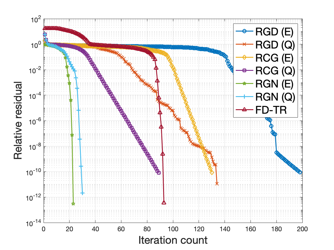
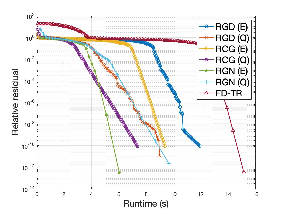
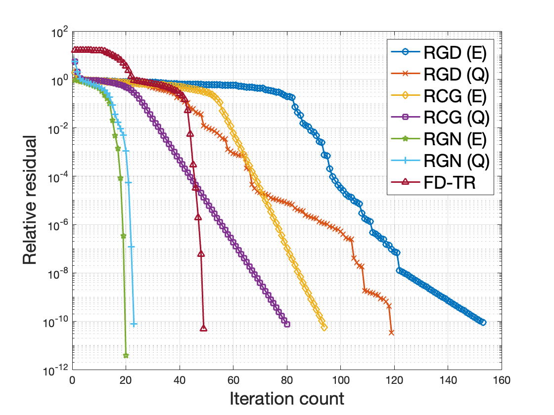
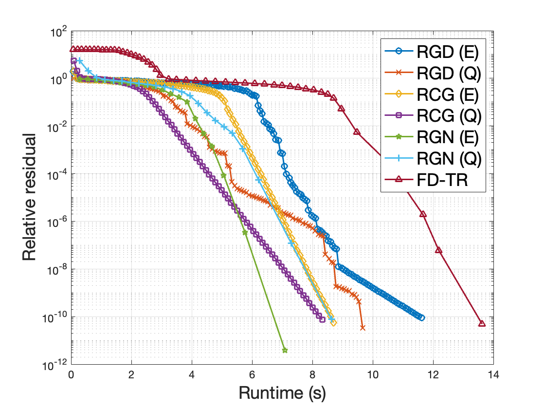
Figure 1: The relative residuals of tested algorithms with respect to the iteration count and runtime (in seconds). Top panels: $\operatorname{OS}=15$; bottom panels: $\operatorname{OS}=20$.

While random tensors have benign condition numbers, we also compare the performance of the tested algorithms under a higher condition number $\kappa=600$. We set $d=9$, $n_{1}=n_{2}=\cdots=n_{9}=5$, $\bm{r}=(1,3,5,10,10,10,10,5,3,1)$, $\operatorname{OS}=\left\{15,20\right\}$. The random tensors with fixed condition number are generated in the same way as in Section 4.1. Tested algorithms are terminated whenever the relative residual $\frac{\left\|{\cal P}_{\Omega}\left({\cal X}_{t}\right)-{\cal P}_{\Omega}\left({\cal T}\right)\right\|_{{\footnotesize{\mathsf{F}}}}}{\left\|{\cal P}_{\Omega}\left({\cal T}\right)\right\|_{{\footnotesize{\mathsf{F}}}}}$ is less than $10^{-10}$ or $250$ number of iterations are reached. In Figure 2, we show the relative residual of each algorithm against the number of iteration and runtime. In this setting, the algorithms proposed in this paper are computationally more efficient than other state-of-the-art algorithms. Moreover, it can be observed that RGD (Q) and RCG (Q) have a rapid initial residual decrease even when the condition number is large. Thus, the total number of iterations for them to converge rely weakly on the condition number. In contrast, the convergence of RGD (E) and RCG (E) relies heavily on the condition number of test tensors.

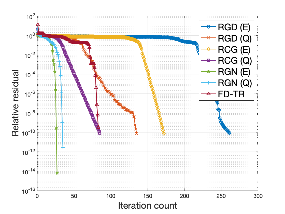
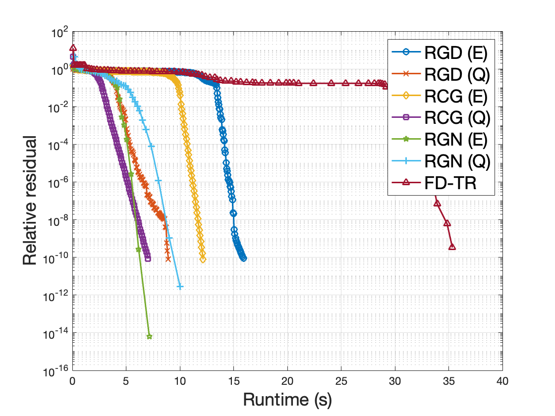
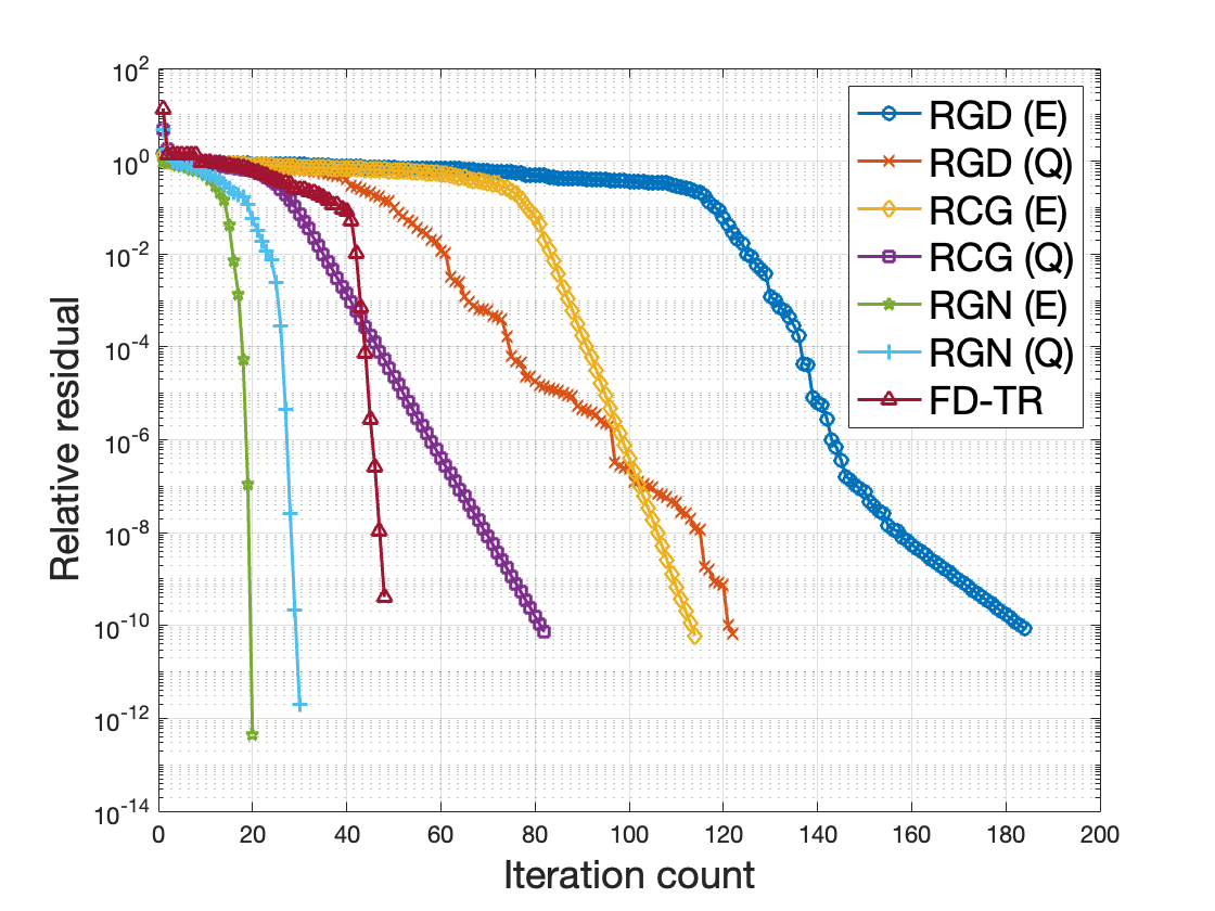
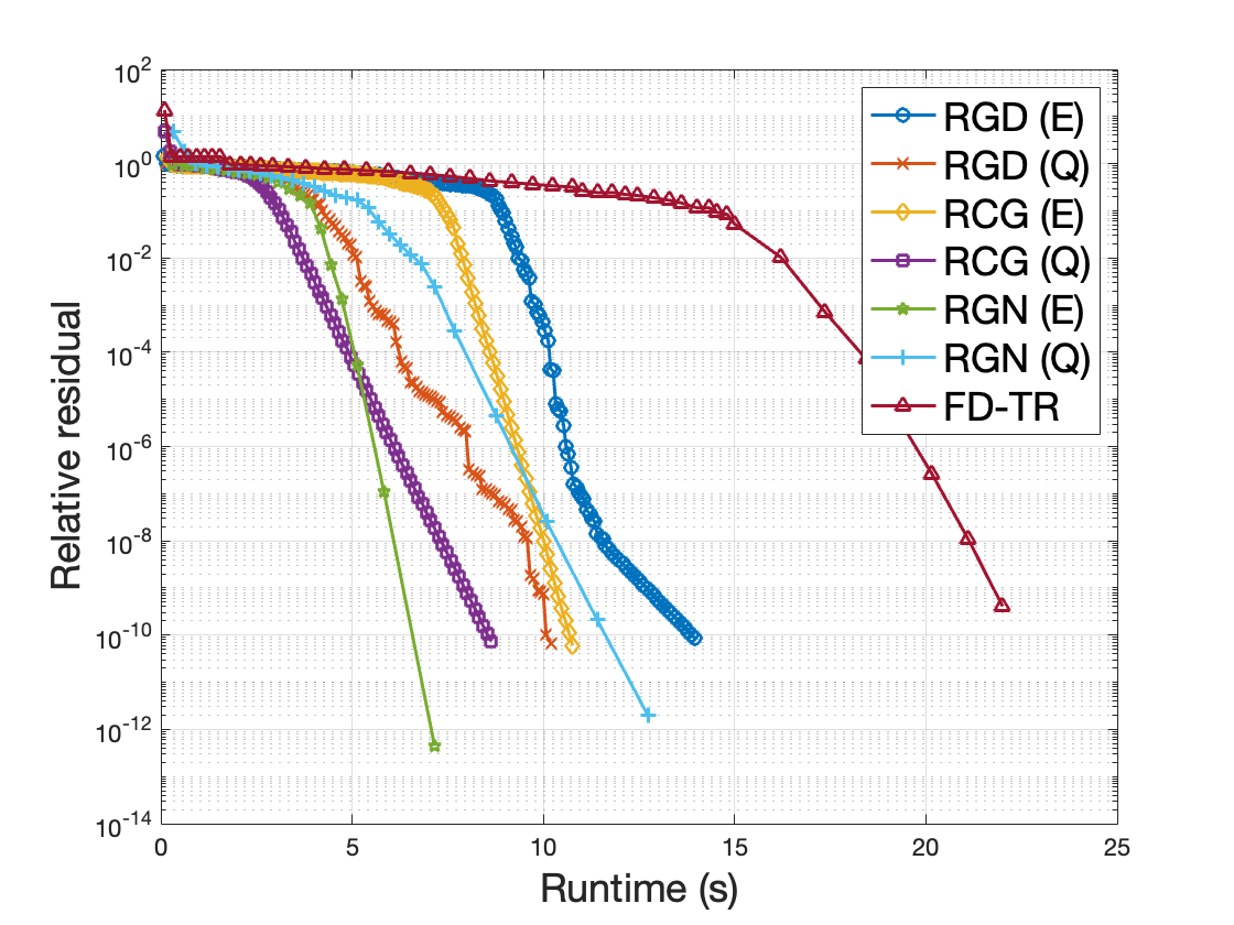
Figure 2: The relative residuals of tested algorithms with respect to the iteration count and runtime (in seconds) under condition number $\kappa=600$. Top panels: $\operatorname{OS}=15$; bottom panels: $\operatorname{OS}=20$.

4.3 Interpolation of High Dimensional Functions

Lastly, we compare the performance of the tested algorithms on two discretization tensors of function data which were tested in [27]. The ground truth tensor ${\cal T}_{1}\in\mathbb{R}^{n_{1}\times\cdots\times n_{d}}$ is constructed by

$${\cal T}_{1}\left(i_{1},\cdots,i_{d}\right)=\exp\left(-\sqrt{\sum_{k=1}^{d}\left(\frac{i_{k}}{n_{k}-1}\right)^{2}}\right),$$

while the other tensor ${\cal T}_{2}\in\mathbb{R}^{n_{1}\times\cdots\times n_{d}}$ is generated by

$${\cal T}_{2}\left(i_{1},\cdots,i_{d}\right)=\frac{1}{\sqrt{\sum_{k=1}^{d}i_{k}^{2}}}.$$

We set $d=4$, $n_{1}=n_{2}=n_{3}=n_{4}=20$. The above function-related tensors possess a property that the singular values of their unfolding formats delay sufficiently fast but do not become exactly zero. It implies that the underlying tensors are not precisely low rank. To improve the reconstruction quality for these data, we adopt the rank-increasing strategy proposed in [27] for the tested algorithms. For more details about the rank-increasing procedure, we refer the reader to [27, Section 4.9]. The maximum rank is set to $\bm{r}=\left(1,5,5,5,1\right)$. Tested algorithms are terminated at each rank-increasing step whenever the relative residual $\frac{\left\|{\cal P}_{\Omega}\left({\cal X}_{t}\right)-{\cal P}_{\Omega}\left({\cal T}\right)\right\|_{{\footnotesize{\mathsf{F}}}}}{\left\|{\cal P}_{\Omega}\left({\cal T}\right)\right\|_{{\footnotesize{\mathsf{F}}}}}$ is less than $10^{-5}$, or $15$ ($20$ at final step) number of iterations are reached, or the relative change $\frac{|\left\|{\cal P}_{\Omega}\left({\cal X}_{t}\right)-{\cal P}_{\Omega}\left({\cal T}\right)\right\|_{{\footnotesize{\mathsf{F}}}}-\left\|{\cal P}_{\Omega}\left({\cal X}_{t-1}\right)-{\cal P}_{\Omega}\left({\cal T}\right)\right\|_{{\footnotesize{\mathsf{F}}}}|}{\left\|{\cal P}_{\Omega}\left({\cal X}_{t-1}\right)-{\cal P}_{\Omega}\left({\cal T}\right)\right\|_{{\footnotesize{\mathsf{F}}}}}$ is less than $10^{-3}$.

The computational results show that the second-order methods with the rank-increasing strategy do not have a good performance on this task. Thus, we only present the results for the first-order methods under different sizes of sampling set $\Omega$ in Table 2. As in [27], the relative test error on a randomly sampling set $\Gamma$ (outside of $\Omega$) with $|\Gamma|=100$ is reported, which is defined by $\frac{\left\|{\cal P}_{\Gamma}\left({\cal X}_{t}\right)-{\cal P}_{\Gamma}\left({\cal T}\right)\right\|_{{\footnotesize{\mathsf{F}}}}}{\left\|{\cal P}_{\Gamma}\left({\cal T}\right)\right\|_{{\footnotesize{\mathsf{F}}}}}$. From the table, we can see that all the four algorithms achieve the overall similar performance.

Table 2: Comparison of the reconstruction quality of RGD (E), RGD (Q), RCG (E), RCG (Q) under different sizes of sampling set for underlying tensors ${\cal T}_{1}$ and ${\cal T}_{2}$.

		underlying tensor ${\cal T}_{1}$			underlying tensor ${\cal T}_{2}$
	$|\Omega|/n^{d}$	0.001	0.01	0.1	0.001	0.01	0.1
RGD (E)	relative error	9.13e-2	2.60e-3	1.21e-4	1.17e-0	8.89e-2	5.07e-4
	runtime (s)	1.01	1.31	1.25	1.36	1.31	1.53
	iteration count	122	121	57	140	124	73
RGD (Q)	relative error	1.05e-1	2.60e-3	1.40e-4	2.16e-1	5.80e-2	5.33e-4
	runtime (s)	0.74	0.98	1.24	0.94	1.01	1.42
	iteration count	114	128	67	140	136	79
RCG (E)	relative error	9.60e-2	1.20e-3	8.09e-5	9.76e-1	7.23e-2	5.62e-4
	runtime (s)	0.55	0.89	1.04	0.65	0.93	1.24
	iteration count	99	111	45	122	124	56
RCG (Q)	relative error	1.03e-1	1.20e-3	8.07e-5	1.80e-1	8.30e-3	5.57e-4
	runtime (s)	0.58	0.93	1.18	0.62	0.98	1.44
	iteration count	96	115	51	100	127	64

5 Conclusion and Future Directions

In this paper, we study the quotient geometry of the manifold of fixed tensor train rank tensors under a preconditioned metric. Algorithms, including Riemannian gradient descent, Riemannian conjugate descent, and Riemannian Gauss-Newton, have been proposed for the tensor completion problem based on the quotient geometry. It has been empirically demonstrated that the proposed algorithms are competitive with other existing algorithms on random tensors as well as function-related tensors in terms of recovery ability, convergence performance, and reconstruction quality.

There are a few lines of research for future directions. First, we would like to establish theoretical recovery guarantees of the proposed algorithms for the low tensor train rank tensor completion problem. Apart from that, it is also interesting to design efficient algorithms for the tensor robust principal component analysis (RPCA) problem under the quotient geometry based on the tensor train format. Furthermore, it is likely to study the quotient geometry of the low-rank hierarchical Tucker tensors under the preconditioned metric studied in this paper.

References

- [1] P-A Absil, Robert Mahony, and Rodolphe Sepulchre. Optimization algorithms on matrix manifolds. Princeton University Press, 2009.
- [2] Anima Anandkumar, Dean P Foster, Daniel Hsu, Sham M Kakade, and Yi-Kai Liu. A spectral algorithm for latent dirichlet allocation. Algorithmica, 72(1):193–214, 2015.
- [3] Johann A Bengua, Ho N Phien, Hoang Duong Tuan, and Minh N Do. Efficient tensor completion for color image and video recovery: Low-rank tensor train. IEEE Transactions on Image Processing, 26(5):2466–2479, 2017.
- [4] Nicolas Boumal. An introduction to optimization on smooth manifolds. Available online, May, 3, 2020.
- [5] Nicolas Boumal, Bamdev Mishra, P-A Absil, and Rodolphe Sepulchre. Manopt, a matlab toolbox for optimization on manifolds. The Journal of Machine Learning Research, 15(1):1455–1459, 2014.
- [6] Jian-Feng Cai, Jingyang Li, and Dong Xia. Provable tensor-train format tensor completion by riemannian optimization. Journal of Machine Learning Research, 23(123):1–77, 2022.
- [7] Andrzej Cichocki, Danilo Mandic, Lieven De Lathauwer, Guoxu Zhou, Qibin Zhao, Cesar Caiafa, and Huy Anh Phan. Tensor decompositions for signal processing applications: From two-way to multiway component analysis. IEEE signal processing magazine, 32(2):145–163, 2015.
- [8] Curt Da Silva and Felix J Herrmann. Optimization on the hierarchical tucker manifold–applications to tensor completion. Linear Algebra and its Applications, 481:131–173, 2015.
- [9] Shuyu Dong, Bin Gao, Wen Huang, and Kyle A Gallivan. On the analysis of optimization with fixed-rank matrices: a quotient geometric view. arXiv preprint arXiv:2203.06765, 2022.
- [10] Jean Gallier et al. The schur complement and symmetric positive semidefinite (and definite) matrices (2019). URL https://www. cis. upenn. edu/jean/schur-comp. pdf, 2020.
- [11] Jean Charles Gilbert and Jorge Nocedal. Global convergence properties of conjugate gradient methods for optimization. SIAM Journal on optimization, 2(1):21–42, 1992.
- [12] Wolfgang Hackbusch and Stefan Kühn. A new scheme for the tensor representation. Journal of Fourier analysis and applications, 15(5):706–722, 2009.
- [13] Frank L Hitchcock. The expression of a tensor or a polyadic as a sum of products. Journal of Mathematics and Physics, 6(1-4):164–189, 1927.
- [14] Sebastian Holtz, Thorsten Rohwedder, and Reinhold Schneider. On manifolds of tensors of fixed tt-rank. Numerische Mathematik, 120(4):701–731, 2012.
- [15] Bruno Iannazzo and Margherita Porcelli. The riemannian barzilai–borwein method with nonmonotone line search and the matrix geometric mean computation. IMA Journal of Numerical Analysis, 38(1):495–517, 2018.
- [16] Alexandros Karatzoglou, Xavier Amatriain, Linas Baltrunas, and Nuria Oliver. Multiverse recommendation: n-dimensional tensor factorization for context-aware collaborative filtering. In Proceedings of the fourth ACM conference on Recommender systems, pages 79–86, 2010.
- [17] Hiroyuki Kasai and Bamdev Mishra. Low-rank tensor completion: a riemannian manifold preconditioning approach. In International Conference on Machine Learning, pages 1012–1021. PMLR, 2016.
- [18] Ji Liu, Przemyslaw Musialski, Peter Wonka, and Jieping Ye. Tensor completion for estimating missing values in visual data. IEEE transactions on pattern analysis and machine intelligence, 35(1):208–220, 2012.
- [19] Christian Lubich, Ivan V Oseledets, and Bart Vandereycken. Time integration of tensor trains. SIAM Journal on Numerical Analysis, 53(2):917–941, 2015.
- [20] Bamdev Mishra, K Adithya Apuroop, and Rodolphe Sepulchre. A riemannian geometry for low-rank matrix completion. arXiv preprint arXiv:1211.1550, 2012.
- [21] Bamdev Mishra and Rodolphe Sepulchre. Riemannian preconditioning. SIAM Journal on Optimization, 26(1):635–660, 2016.
- [22] Ivan V Oseledets. Tensor-train decomposition. SIAM Journal on Scientific Computing, 33(5):2295–2317, 2011.
- [23] Michael Psenka and Nicolas Boumal. Second-order optimization for tensors with fixed tensor-train rank. arXiv preprint arXiv:2011.13395, 2020.
- [24] Alfio Quarteroni, Riccardo Sacco, and Fausto Saleri. Numerical mathematics, volume 37. Springer Science & Business Media, 2010.
- [25] Holger Rauhut, Reinhold Schneider, and Željka Stojanac. Low rank tensor recovery via iterative hard thresholding. Linear Algebra and its Applications, 523:220–262, 2017.
- [26] Ulrich Schollwöck. The density-matrix renormalization group in the age of matrix product states. Annals of physics, 326(1):96–192, 2011.
- [27] Michael Steinlechner. Riemannian optimization for high-dimensional tensor completion. SIAM Journal on Scientific Computing, 38(5):S461–S484, 2016.
- [28] Ledyard R Tucker. Some mathematical notes on three-mode factor analysis. Psychometrika, 31(3):279–311, 1966.
- [29] André Uschmajew and Bart Vandereycken. The geometry of algorithms using hierarchical tensors. Linear Algebra and its Applications, 439(1):133–166, 2013.
- [30] André Uschmajew and Bart Vandereycken. Geometric methods on low-rank matrix and tensor manifolds. In Handbook of variational methods for nonlinear geometric data, pages 261–313. Springer, 2020.
- [31] Frank Verstraete, Valentin Murg, and J Ignacio Cirac. Matrix product states, projected entangled pair states, and variational renormalization group methods for quantum spin systems. Advances in physics, 57(2):143–224, 2008.
- [32] Junli Wang, Guangshe Zhao, Dingheng Wang, and Guoqi Li. Tensor completion using low-rank tensor train decomposition by riemannian optimization. In 2019 Chinese Automation Congress (CAC), pages 3380–3384. IEEE, 2019.
- [33] Longhao Yuan, Qibin Zhao, and Jianting Cao. Completion of high order tensor data with missing entries via tensor-train decomposition. In International Conference on Neural Information Processing, pages 222–229. Springer, 2017.
- [34] Shixin Zheng, Wen Huang, Bart Vandereycken, and Xiangxiong Zhang. Riemannian optimization using three different metrics for hermitian psd fixed-rank constraints: an extended version. arXiv preprint arXiv:2204.07830, 2022.