Asymmetric Dark Matter from Gravitational Waves

Abstract

We investigate the prospects for probing asymmetric dark matter models through their gravitational wave signatures. We concentrate on a theory extending the Standard Model gauge symmetry by a non-Abelian group, under which leptons form doublets with new fermionic partners, one of them being a dark matter candidate. The breaking of this new symmetry occurs at a high scale, and results in a strong first order phase transition in the early Universe. The model accommodates baryogenesis in an asymmetric dark matter setting and predicts a gravitational wave signal within the reach of near-future experiments.

I Introduction

In the past several decades, theoretical and experimental particle physics have brought us incredible insight into how the Universe works at the most fundamental level, with our current knowledge extending down to distances $\sim 10^{-18}\ \rm m$. The Standard Model of elementary particles, formulated in the 1960s Glashow (1961); Higgs (1964); Englert and Brout (1964); Weinberg (1967); Salam (1968) and 1970s Fritzsch et al. (1973); Gross and Wilczek (1973); Politzer (1973), provides the most comprehensive description of physics at such small scales, with the last piece of the puzzle, the Higgs boson, discovered a decade ago at the Large Hadron Collider (LHC) Chatrchyan et al. (2012). Although currently accessible sporadically only in high-energy environments, particle physics effects were not always so elusive. Cosmological observations indicate that the Universe is expanding and started off from a state with a large density and temperature, when it was precisely the physics at the small scale that drove its evolution. This introduces additional motivation for exploring particle physics models, especially in light of the fact that several fundamental questions still remain unanswered. Among the most pressing open issues are the nature of dark matter and the origin of the matter-antimatter asymmetry of the Universe, which both require the existence of new physics, i.e., particles and interactions beyond those described by the Standard Model.

Observations indicate that there is five times more matter in the Universe than what can be attributed to visible matter. The existence of this dark matter was inferred from its gravitational interaction with normal matter, first from applying the virial theorem to a galaxy cluster Zwicky (1933); Andernach and Zwicky , and then through the measurements of galactic rotation curves Rubin and Ford (1970). By now, the evidence for dark matter in the Universe is overwhelming, with its distribution and abundance precisely determined also from the cosmic microwave background de Bernardis et al. (2000) and gravitational lensing Gavazzi et al. (2007). Despite those huge advances, the mass of the dark matter particle and its non-gravitational interactions with the Standard Model remain a mystery. It is not even known if the dark matter consists of individual particles or whether it is made up of macroscopic objects like dark quark nuggets Bai et al. (2019) or primordial black holes Carr et al. (2010); Bird et al. (2016). The allowed masses for particle dark matter span an extremely wide range of values, starting from very small ones like in the case of fuzzy dark matter Press et al. (1990); Hui et al. (2017), through intermediate ones like for standard weakly interacting massive particles (WIMPs) Steigman and Turner (1985), up to very large masses for WIMPzillas Kolb et al. (1999); Meissner and Nicolai (2019). For a review of particle dark matter candidates, see Feng (2010) and references therein.

In the matter-antimatter asymmetry problem, the question is how at some point in the early Universe there happened to be slightly more matter than antimatter, despite both being produced in equal amounts during post-inflationary reheating. The minimal conditions needed to achieve this include out-of-equilibrium dynamics, as well as violation of baryon number, charge and the charge-parity symmetry Sakharov (1967). A very attractive class of theories is singled out if one assumes that the ordinary and dark sectors share a common origin. Such a connection is hinted by the fact that the abundances of dark matter and ordinary matter are roughly of the same order. This observation lies at the heart of theories of asymmetric dark matter Nussinov (1985); Kaplan (1992); Hooper et al. (2005); Kaplan et al. (2009); Petraki and Volkas (2013); Zurek (2014), in which the asymmetries in the dark and visible sectors are generated simultaneously, and the natural mass scale for the dark matter particle is on the order of the proton mass. Apart from the GeV-scale dark matter candidate itself, models of asymmetric dark matter contain new heavy particles, which determine the properties of the out-of-equilibrium dynamics. In order to gain access to those heavy states, one would need to construct higher-energy accelerators, much more powerful than the LHC. However, recently a novel and very promising method of probing such particle physics models emerged.

The first detection of gravitational waves by the Laser Interferometer Gravitational Wave Observatory within the LIGO/Virgo collaboration Abbott et al. (2016) was a milestone discovery, made one century after the predictions of general relativity Einstein (1916), and initiated a renaissance period for gravitational wave astronomy. Although only signals arising from black hole and neutron star mergers have been observed thus far, a primordial stochastic gravitational wave background carrying information about the very early period in the evolution of the Universe can also be searched for by the LIGO/Virgo/KAGRA (LVK) detectors. Indeed, such a stochastic gravitational wave background could have been produced in several cosmological processes, including first order phase transitions in the early Universe Kosowsky et al. (1992) and inflation Turner (1997), or through the dynamics of topological defects like cosmic strings Vachaspati and Vilenkin (1985); Sakellariadou (1990) and domain walls Hiramatsu et al. (2010). In this study, we focus on gravitational waves from phase transitions. The LVK detectors’ frequency range coincides with the scale of new physics triggering the first order phase transition $\sim\mathcal{O}(10\!-\!100)\ {\rm PeV}$. This reach will extend towards lower scales and have better sensitivity with future experiments like the Laser Interferometer Space Antenna Amaro-Seoane et al. (2017), Einstein Telescope Punturo et al. (2010), DECIGO Kawamura et al. (2011), Cosmic Explorer Reitze et al. (2019), and Big Bang Observer Crowder and Cornish (2005).

The origin of the stochastic gravitational wave background from first order phase transitions is relatively well-understood. The energy density at each point in the Universe is determined by the minimum of the effective potential, which depends on the details of the particle physics model and the temperature. At high temperatures, the potential has a global minimum located at zero field value (false vacuum). As the Universe cools down, the potential can develop another minimum at a nonzero field value (true vacuum) with a lower energy density than the false vacuum. If a potential barrier separating the two vacua exists, the Universe is temporarily trapped in the false vacuum; however, due to thermal fluctuations or via quantum tunneling, it eventually undergoes a first order phase transition to the true vacuum. This process corresponds to nucleating bubbles of true vacuum in different patches of the Universe, which then expand and fill the entire space. For this process to be efficient, the bubble nucleation rate must be larger than the Hubble expansion. The nucleation rate is determined by the shape of the effective potential – it depends on the Euclidean bounce action for the expanding bubble solution (saddle point configuration) interpolating between the two vacua. Once the nucleation starts, gravitational waves are generated from bubble wall collisions, sound waves in the plasma, and magnetohydrodynamic turbulence.

At the particle physics level, a first order phase transition is triggered by spontaneous symmetry breaking. Many attractive extensions of the Standard Model exhibit an increased symmetry of the Lagrangian at high energies, which breaks down to ${\rm SU}(3)_{c}\times{\rm SU}(2)_{L}\times{\rm U}(1)_{Y}$ at low energies. Given the expected gravitational wave signatures of first order phase transitions, detectors like LVK and future gravitational wave experiments are in a great position to test such theories. Indeed, a plethora of particle physics models experiencing spontaneous symmetry breaking have already been explored in the literature regarding their gravitational wave signatures from first order phase transitions (see Caldwell et al. (2022) and references therein), including theories with new physics at the electroweak scale Grojean and Servant (2007); Vaskonen (2017); Dorsch et al. (2017); Bernon et al. (2018); Baldes and Servant (2018); Chala et al. (2018); Alves et al. (2019); Han et al. (2021); Azatov et al. (2021); Benincasa et al. (2022), neutrino seesaw models Brdar et al. (2019); Okada and Seto (2018); Di Bari et al. (2021); Zhou et al. (2022), baryon/lepton number violation Baldes (2017); Hasegawa et al. (2019); Fornal and Shams Es Haghi (2020)), grand unified theories Croon et al. (2019); Huang et al. (2020); Okada et al. (2021), dark gauge groups Schwaller (2015); Breitbach et al. (2019); Croon et al. (2018); Hall et al. (2020), models with conformal invariance Ellis et al. (2020a); Kawana (2022), axions Dev et al. (2019); Von Harling et al. (2020); Delle Rose et al. (2020), supersymmetry Craig et al. (2020); Fornal et al. (2021), and new flavor physics Greljo et al. (2020); Fornal (2021).

Models providing explanations for the matter-antimatter asymmetry of the Universe are particularly good candidates to search for in gravitational wave experiments, since the out-of-equilibrium dynamics needed to generate the baryon asymmetry is usually triggered by a first order phase transition, which is precisely one of the processes expected to result in a stochastic gravitational wave background. Such signatures have been investigated in the case of electroweak baryogenesis models, in which new states appear at the scale of hundreds of GeV Vaskonen (2017); Dorsch et al. (2017); Baldes (2017). In this paper we focus our investigation on theories of asymmetric dark matter with new states at the PeV scale rather than the electroweak scale. This shifts the expected signal to future sensitivity regions of the Einstein Telescope and Cosmic Explorer. For concreteness, we perform our analysis based on the theory introduced in Fornal et al. (2017), in which baryon number violation proceeds through a new type of instanton interactions arising from the non-Abelian nature of the gauge extension of the Standard Model. The model not only exhibits a strong first order phase transition, but also predicts the formation of domain walls in the early Universe.

II Model

The model we consider Fornal et al. (2017) is based on the gauge group

$${\rm SU}(3)_{c}\times{\rm SU}(2)_{L}\times{\rm U}(1)_{Y}\times{\rm SU}(2)_{\ell}\ .$$ (1)

The quarks are singlets under ${\rm SU}(2)_{\ell}$, whereas the leptons are the upper components of ${\rm SU}(2)_{\ell}$ doublets. Denoting the new fields, other than the right-handed neutrinos, by tildes and primes, the leptonic fields of the model (for each family) have the following quantum numbers under the group in Eq. (1):

$$(l_{L}\ \ \ \tilde{l}_{L})^{T}\,\equiv\ \,\hat{l}_{L} = (1,2,-\tfrac{1}{2},2)\ ,\ \ \ l^{\prime}_{R}=(1,2,-\tfrac{1}{2},1)\ ,\ \ \ \$$

$$(e_{R}\ \ \tilde{e}_{R})^{T}\equiv\ \hat{e}_{R} = (1,1,-1,2)\ ,\ \ \ e^{\prime}_{L}=(1,1,-1,1)\ ,$$

$$(\nu_{R}\ \ \tilde{\nu}_{R})^{T}\equiv\ \hat{\nu}_{R} = (1,1,0,2)\ ,\ \ \ \ \ \ \nu^{\prime}_{L}=(1,1,0,1)\ .$$ (2)

In order to spontaneously break ${\rm SU}(2)_{\ell}$ and accommodate a successful mechanism for baryogenesis, two complex ${\rm SU}(2)_{\ell}$ doublet scalar fields are introduced, $\Phi_{1}$ and $\Phi_{2}$. The general form of the scalar potential is given by

$$V(\Phi_{1},\Phi_{2})=m_{1}^{2}|\Phi_{1}|^{2}+m_{2}^{2}|\Phi_{2}|^{2}-(m_{12}^{2}\Phi_{1}^{\dagger}\Phi_{2}+{\rm h.c.})$$ (3)

$$+ \lambda_{1}|\Phi_{1}|^{4}+\lambda_{2}|\Phi_{2}|^{4}+\lambda_{3}|\Phi_{1}|^{2}|\Phi_{2}|^{2}+\lambda_{4}|\Phi_{1}^{\dagger}\Phi_{2}|^{2}$$

$$+ \big{[}\big{(}\tilde{\lambda}_{5}|\Phi_{1}|^{2}+\tilde{\lambda}_{6}|\Phi_{2}|^{2}+\tilde{\lambda}_{7}\Phi_{1}^{\dagger}\Phi_{2}\big{)}\Phi_{1}^{\dagger}\Phi_{2}+{\rm h.c.}\big{]}\ ,\ \ \$$

where the parameters $m_{12}^{2}$, $\tilde{\lambda}_{5}$, $\tilde{\lambda}_{6}$, and $\tilde{\lambda}_{7}$ are complex. The scalar fields $\Phi_{1}$ and $\Phi_{2}$ develop vacuum expectation values (vevs) $v_{1}$ and $v_{2}$, respectively, upon which the ${\rm SU}(2)_{\ell}$ symmetry is broken and one is left with the Standard Model gauge group. Those fields can be written as

$$\Phi_{j}=\begin{pmatrix}c_{1j}+ic_{2j}\\ \frac{1}{\sqrt{2}}(v_{j}+p_{j}+ia_{j})\end{pmatrix}$$ (4)

for $j=1,2$, where $p_{j}$, $a_{j}$, $c_{1j}$ and $c_{2j}$ are real fields. To simplify the notation, we introduce the parameters

$$v_{\ell}\equiv\sqrt{v_{1}^{2}+v_{2}^{2}}\ ,\ \ \ \ \ \tan\beta\equiv\frac{v_{2}}{v_{1}}\ .$$ (5)

In the regime $v_{\ell}\sim\mathcal{O}(1-1000)\ {\rm PeV}$, the LEP-II experimental bound $v_{\ell}\gtrsim 1.7\ {\rm TeV}$ Schwaller et al. (2013) is easily satisfied.

The Yukawa interactions in the model are given by

$$\mathcal{L}_{\rm Y} = \sum_{j}\Big{(}Y_{l}^{ab}\,\bar{\hat{l}}_{L}^{a}\,\hat{\Phi}_{j}\,{l^{\prime}}_{\!\!R}^{b}+Y_{e}^{ab}\,\bar{\hat{e}}_{R}^{a}\,\hat{\Phi}_{j}\,{e^{\prime}}_{\!\!L}^{b}+Y_{\nu}^{ab}\,\bar{\hat{\nu}}_{R}^{a}\,\hat{\Phi}_{j}\,{\nu^{\prime}}_{\!\!L}^{b}\Big{)}$$ (6)

$$+ y_{e}^{ab}\,\bar{\hat{l}}_{L}^{a}\,H\,\hat{e}_{R}^{b}+y_{\nu}^{ab}\,\bar{\hat{l}}_{L}^{a}\,\tilde{H}\,\hat{\nu}_{R}^{b}+{y^{\prime}}_{\!\!e}^{ab}\,\bar{l^{\prime}}_{\!\!R}^{a}\,H\,{e^{\prime}}_{\!\!L}^{b}$$

$$+ {{y^{\prime}}}_{\!\!\nu}^{ab}\,\bar{l^{\prime}}_{\!\!R}^{a}\,\tilde{H}\,{\nu^{\prime}}_{\!\!L}^{b}+{\rm h.c.}\ ,$$

with an implicit sum over the flavor indices $a,b$. The terms in the first line of Eq. (6), involving the matrices $Y_{l}$, $Y_{e}$ and $Y_{\nu}$, result in vector-like masses for the new fermions. The Yukawa matrices $y_{e}$ and $y_{\nu}$ provide masses to the Standard Model charged leptons and neutrinos, whereas $y^{\prime}_{e}$ and $y^{\prime}_{\nu}$ lead to an additional contribution to the new fermion masses. Under the phenomenologically natural assumption,

$$Y_{l,e,\nu}v_{\ell}\gg y_{l,e,\nu}\,v_{H}\ ,\ \ \ \ Y_{l,e,\nu}v_{\ell}\gg y^{\prime}_{l,e,\nu}v_{H}\ ,$$ (7)

where $v_{H}$ is the Higgs vev, all constraints from electroweak precision data are satisfied.

After ${\rm SU}(2)_{\ell}$ breaking, there exist six electrically charged and six neutral new fermionic states $f^{\prime}$. It was demonstrated in Fornal et al. (2017) that a remnant ${\rm U}(1)_{\ell}$ symmetry forbids the new fermions from decaying to Standard Model particles. As a result, if the lightest of those states, say $\chi$, is electrically neutral, it becomes a good dark matter candidate. The condition in Eq. (7) assures that the electroweak doublet contribution to $\chi$ is small, and, to a good approximation,

$$\chi_{L}\approx\nu^{\prime}_{L}\ ,\ \ \ \ \chi_{R}\approx\tilde{\nu}_{R}\ .$$ (8)

For simplicity, we assume that the elements of the matrices $Y_{l}$, $Y_{e}$ and $Y_{\nu}$ are small, $(Y_{l,e,\nu})_{ij}\ll 1$. Nevertheless, given the $\sim\mathcal{O}(10)\,\rm PeV$ symmetry breaking scale, the masses of the new fermions can still be large. In particular, one may envision a scenario with 11 heavy new fermions with masses $m_{f^{\prime}}\sim\mathcal{O}(1)\,{\rm PeV}$ and one light dark matter state $\chi$ with mass $m_{\chi}\approx 5\ {\rm GeV}$ (see Sec. IV).

The gauge sector contains three new vector gauge bosons: $Z^{\prime}$, $W^{\prime}_{1}$, and $W^{\prime}_{2}$. Denoting by $g_{\ell}$ the ${\rm SU}(2)_{\ell}$ gauge coupling, their masses are

$$m_{Z^{\prime}\!,W^{\prime}_{1,2}}=\tfrac{1}{2}\,g_{\ell}\,v_{\ell}\ .$$ (9)

The new gauge bosons have no direct couplings to quarks, so there do not exist any unsuppressed tree-level diagrams contributing to dark matter direct detection. Although processes relevant for direct detection do arise at the loop level, the resulting limits set by the CDMSlite experiment Agnese et al. (2016) are much weaker than the aforementioned LEP-II constraint.

The scalar content of the theory consists of two real $CP$-even states, one real $CP$-odd state, and two complex conjugated states, which we denote respectively by

$$P_{1},\ P_{2}\ ,A\ ,C_{1}\ ,C_{2}\ .$$ (10)

Their masses depend on the parameters of the scalar potential in Eq. (3) and, without tuning, are naturally at the scale $\sim v_{\ell}$. As argued in Sec. IV, the $CP$-odd scalar $A$ is chosen to be lighter than $\chi$, so that there exist efficient dark matter annihilation channels. The field-dependent masses for all those particles are discussed in Sec. III, including the ones for the three Goldstone bosons $G$, $G_{1}$, and $G_{2}$.

III Effective potential

In order to investigate the dynamics of the phase transition, one needs to determine the shape of the effective potential. In contrast to Fornal et al. (2017), in this work we will not assume $v_{1}\gg v_{2}$. Given the large number of parameters, to make our analysis more transparent we set $\lambda_{3},\lambda_{4},\tilde{\lambda}_{5},\tilde{\lambda}_{6}=0$. The conditions required for vacuum stability reduce then to

$$\lambda_{1},\lambda_{2}>0\ \ \ \ {\rm and}\ \ \ \ |\tilde{\lambda}_{7}|<\sqrt{\lambda_{1}\lambda_{2}}\ .\ \ \ \ \$$ (11)

With a small nonzero parameter $m_{12}^{2}$, the theory exhibits a softly broken $\mathcal{Z}_{2}$ symmetry defined by the transformation

$$\Phi_{1}\to\Phi_{1}\ ,\ \ \ \Phi_{2}\to-\Phi_{2}\ .$$ (12)

The effective potential is a function of the classical background fields $(\phi_{1},\phi_{2})$ and consists of 3 contributions: tree-level, one-loop Coleman-Weinberg, and finite temperature,

$$V_{\rm eff}(\phi_{1},\phi_{2},T)$$ (13)

$$= V_{\rm tree}(\phi_{1},\phi_{2})+V_{\rm loop}(\phi_{1},\phi_{2})+V_{\rm temp}(\phi_{1},\phi_{2},T)\ .\ \ \ \ \ \ \ \$$

The tree-level contribution, upon expressing the parameters $\mu_{1}^{2}$ and $\mu_{2}^{2}$ in terms of $v_{\ell}$, $\beta$, $\mu_{12}^{2}$ and $\tilde{\lambda}_{7}$ using the minimization conditions, takes the form

$$V_{\rm tree}(\phi_{1},\phi_{2})=\tfrac{1}{4}\lambda_{1}\phi_{1}^{4}+\tfrac{1}{4}\lambda_{2}\phi_{2}^{4}-\mu_{12}^{2}\phi_{1}\phi_{2}+\tfrac{1}{2}\lambda_{7}\phi_{1}^{2}\phi_{2}^{2}$$ (14)

$$+ \tfrac{1}{2}\big{[}\,\mu^{2}_{12}\tan\!\beta-\lambda_{1}v_{\ell}^{2}\cos^{2}\!\beta-\lambda_{7}v_{\ell}^{2}\sin^{2}\!\beta\big{]}\phi_{1}^{2}\ \$$

$$+ \tfrac{1}{2}\big{[}\,\mu^{2}_{12}\cot\!\beta-\lambda_{2}v_{\ell}^{2}\sin^{2}\!\beta-\lambda_{7}v_{\ell}^{2}\cos^{2}\!\beta\big{]}\phi_{2}^{2}\ ,$$

where $\mu_{12}^{2}={\rm Re}(m_{12}^{2})$ and $\lambda_{7}={\rm Re}(\tilde{\lambda}_{7})$. Adopting the $\overline{\rm MS}$ renormalization scheme, the Coleman-Weinberg term is Quiros (1999)

$$\!\!\!\!\!\!\!V_{\rm loop}(\phi_{1},\phi_{2})$$ (15)

$$= \sum_{i}\frac{n_{i}}{64\pi^{2}}m_{i}^{4}(\phi_{1},\phi_{2})\left[\log\left(\frac{m_{i}^{2}(\phi_{1},\phi_{2})}{\Lambda^{2}}\right)-c_{i}\right]\!,\ \ \ \ \ \ \ \$$

where the sum includes all particles charged under ${\rm SU}(2)_{\ell}$, $m_{i}(\phi_{1},\phi_{2})$ are their field-dependent masses, $n_{i}$ denotes their number of degrees of freedom (with a negative sign for fermions), $c_{i}=3/2$ for fermions and scalars, $c_{i}=5/6$ for vector bosons, and $\Lambda$ is the renormalization scale.

For the gauge bosons in the theory, the squared field-dependent masses are

$$m_{Z^{\prime}\!,W^{\prime}_{1,2}}^{2}(\phi_{1},\phi_{2})=\tfrac{1}{4}\,g^{2}_{\ell}(\phi_{1}^{2}+\phi_{2}^{2})\ .$$ (16)

Because of our simplifying assumption regarding the structure of the Yukawa matrices, i.e., $(Y_{l,e,\nu})_{ij}\ll 1$, the field-dependent masses for the fermions are much smaller than those for the gauge bosons, and we will neglect them.

In the case of scalars, the squared field-dependent masses are given by the eigenvalues of three $2\times 2$ matrices: $\mathcal{M}_{P}^{2}$ for the $CP$-even states $P_{1}$ and $P_{2}$,

$$(\mathcal{M}_{P}^{2})_{11} = \lambda_{1}\big{(}3\phi_{1}^{2}-v_{\ell}^{2}\cos^{2}\!\beta\big{)}+\mu_{12}^{2}\tan\!\beta$$

$$+ \lambda_{7}\big{(}\phi_{2}^{2}-v_{\ell}^{2}\sin^{2}\!\beta\big{)}\ ,$$

$$(\mathcal{M}_{P}^{2})_{12} = (\mathcal{M}_{P}^{2})_{21}=2\lambda_{7}\phi_{1}\phi_{2}-\mu_{12}^{2}\ ,$$

$$(\mathcal{M}_{P}^{2})_{22} = \lambda_{2}\big{(}3\phi_{2}^{2}-v_{\ell}^{2}\sin^{2}\!\beta\big{)}+\mu_{12}^{2}\cot\!\beta\ \ \ \ \ \ \ \ \ \ \ \ \ \ \ \$$ (17)

$$+ \lambda_{7}\big{(}\phi_{1}^{2}-v_{\ell}^{2}\cos^{2}\!\beta\big{)}\ ,$$

$\mathcal{M}_{A}^{2}$ for the $CP$-odd state $A$ and the Goldstone boson $G$,

$$(\mathcal{M}_{A}^{2})_{11} = \lambda_{1}\big{(}\phi_{1}^{2}-v_{\ell}^{2}\cos^{2}\!\beta\big{)}+\mu_{12}^{2}\tan\!\beta$$

$$- \lambda_{7}\big{(}\phi_{2}^{2}+v_{\ell}^{2}\sin^{2}\!\beta\big{)}\ ,$$

$$(\mathcal{M}_{A}^{2})_{12} = (\mathcal{M}_{A}^{2})_{21}=2\lambda_{7}\phi_{1}\phi_{2}-\mu_{12}^{2}\ ,$$

$$(\mathcal{M}_{A}^{2})_{22} = \lambda_{2}\big{(}\phi_{2}^{2}-v_{\ell}^{2}\sin^{2}\!\beta\big{)}+\mu_{12}^{2}\cot\!\beta\ \ \ \ \ \ \ \ \ \ \ \ \ \ \ \$$ (18)

$$- \lambda_{7}\big{(}\phi_{1}^{2}+v_{\ell}^{2}\cos^{2}\!\beta\big{)}\ ,$$

and $\mathcal{M}_{C}^{2}$ for the complex states $C_{1,2}$ and the Goldstones $G_{1,2}$,

$$(\mathcal{M}_{C}^{2})_{11} = \lambda_{1}\big{(}\phi_{1}^{2}-v_{\ell}^{2}\cos^{2}\!\beta\big{)}+\mu_{12}^{2}\tan\!\beta-\lambda_{7}\,v_{\ell}^{2}\sin^{2}\!\beta\ ,$$

$$(\mathcal{M}_{C}^{2})_{12} = (\mathcal{M}_{C}^{2})_{21}=2\lambda_{7}\phi_{1}\phi_{2}-\mu_{12}^{2}\ ,$$

$$(\mathcal{M}_{C}^{2})_{22} = \lambda_{2}\big{(}\phi_{2}^{2}-v_{\ell}^{2}\sin^{2}\!\beta\big{)}+\mu_{12}^{2}\cot\!\beta-\lambda_{7}\,v_{\ell}^{2}\cos^{2}\!\beta\ .$$

The finite temperature contribution to the potential is Quiros (1999)

$$V_{\rm temp}(\phi_{1},\phi_{2},T)$$

$$=\frac{T^{4}}{2\pi^{2}}\sum_{i}n_{i}\int_{0}^{\infty}dy\,y^{2}\log\left(1\mp e^{-\sqrt{m_{i}^{2}(\phi_{1},\phi_{2})/T^{2}+y^{2}}}\right)\ \ \ \ \$$

$$+\,\frac{T}{12\pi}\sum_{j}n^{\prime}_{j}\Big{\{}m_{j}^{3}(\phi_{1},\phi_{2})-[m^{2}(\phi_{1},\phi_{2})+\Pi(T)]_{j}^{\frac{3}{2}}\Big{\}}\,,\ \ \ \ \ \$$ (20)

where in the second line the minus sign corresponds to bosons and the plus sign to fermions, the sum over $i$ incorporates all particles with field-dependent masses, the sum over $j$ includes only bosons, $n_{i}$ denotes the number of degrees of freedom for a given particle, $n^{\prime}_{j}$ is the number of all degrees of freedom in the case of scalars and solely longitudinal ones for vector bosons, $\Pi(T)$ is the thermal mass matrix, and $[m^{2}(\phi_{1},\phi_{2})+\Pi(T)]_{j}$ are the eigenvalues of the matrix $[m^{2}(\phi_{1},\phi_{2})+\Pi(T)]$. The $2\times 2$ thermal mass matrix $\Pi(T)$ is diagonal and identical for the four pairs of scalars $(P_{1},P_{2})$, $(A,G)$, $(C_{1},G_{1})$, $(C_{2},G_{2})$. It is given by

$$\Pi(T)=\begin{pmatrix}\frac{3}{16}g_{\ell}^{2}+\tfrac{1}{2}\lambda_{1}&0\\ 0&\tfrac{3}{16}g_{\ell}^{2}+\tfrac{1}{2}\lambda_{2}\end{pmatrix}T^{2}\ .\ \ \ \ \ \ \ \$$ (21)

In the case of vector gauge bosons, the thermal masses are

$$\Pi_{Z^{\prime}}(T)=\Pi_{W^{\prime}_{1,2}}(T)=2g_{\ell}^{2}T^{2}\ .$$ (22)

As an illustration, Fig. 1 presents a slice of the effective potential along the field direction $\phi_{1}=\phi_{2}$ for several different temperatures and for the parameter choice: $\lambda_{1}=\lambda_{2}=10^{-3}$, $\beta=\pi/4$,  $v_{\ell}=\Lambda=10\ \rm PeV$,  $g_{\ell}=1$, and small $|\mu_{12}^{2}|$, $|\lambda_{7}|$.

As the temperature decreases, a new local minimum of the effective potential develops away from the origin. Below the critical temperature $T_{c}$, this minimum, which we denote by $(\phi_{1},\phi_{2})_{\rm true1}$, becomes the new true vacuum of the theory. When the temperature drops further to the so-called nucleation temperature $T_{*}$, patches of the Universe undergo a phase transition to this preferred true vacuum. Since the new vacuum is separated by a potential bump from the false vacuum at the origin, the phase transition is first order. Details of the resulting gravitational wave signal are discussed in Sec. V.

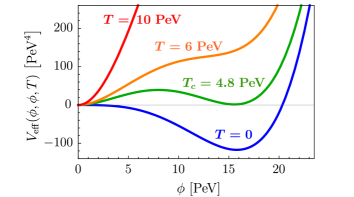
Figure 1: Effective potential $V_{\rm eff}(\phi_{1},\phi_{2},T)$ along the field direction $\phi_{1}=\phi_{2}\equiv\phi$ and normalized to zero at the origin, for the parameter choice discussed in the text and several values of temperature.

The vacuum $(\phi_{1},\phi_{2})_{\rm true1}$ is not the only minimum with energy density lower than that of the false vacuum at the origin. The effective potential develops four minima which come in two pairs – the vacua within each pair are related via the approximate $\mathcal{Z}_{2}$ symmetry of the potential defined in Eq. (12), while the two pairs are related to each other via a gauge symmetry. In particular, they are related through a rephasing transformation of the Lagrangian fields $\Phi_{i}\to e^{i\theta}\Phi_{i}$ ($i=1,2$), making them physically equivalent Ginzburg and Krawczyk (2005). For a detailed discussion of the topology of the scalar potential in two-Higgs doublet models, see Battye et al. (2011).

As a result, there are only two physically distinct true vacua of the theory, $(\phi_{1},\phi_{2})_{\rm true1}$ and $(\phi_{1},-\phi_{2})_{\rm true2}$. Their energy densities differ solely because of the nonzero $\mathcal{Z}_{2}$ symmetry breaking terms in the effective potential, i.e., in our case the term involving the parameter $\mu^{2}_{12}$. If the energy density difference between those two vacua is large, the Universe transitions to the vacuum with lower energy density. However, if the splitting is small, i.e., $|\mu_{12}^{2}|\ll\lambda_{1,2}v_{\ell}^{2}$, then a given patch of the Universe can transition to either $(\phi_{1},\phi_{2})_{\rm true1}$ or $(\phi_{1},-\phi_{2})_{\rm true2}$ , leading to the formation of domain walls Saikawa (2017). Their subsequent annihilation constitutes another possible source of gravitational radiation.

IV Baryogenesis and dark matter

A first order phase transition provides exactly the out-of-equilibrium dynamics needed to generate a matter-antimatter asymmetry of the Universe. The remaining requirements, i.e., violation of baryon number, charge, and the charge-parity symmetry, are also present in the model. As shown in Fornal et al. (2017), this leads to a successful mechanism for baryogenesis, which combines the features of asymmetric dark matter Nussinov (1985); Kaplan (1992); Hooper et al. (2005); Kaplan et al. (2009); Petraki and Volkas (2013); Zurek (2014), Dirac leptogenesis Dick et al. (2000); Murayama and Pierce (2002), and baryon asymmetry generation from an earlier phase transition Shu et al. (2007) (see also Blennow et al. (2011)). In this section, we summarize the most important aspects of this proposal.

Baryon number violation in the model is a result of a lepton number asymmetry produced by the nonperturbative dynamics of ${\rm SU}(2)_{\ell}$ instantons, which remain active outside the expanding bubble of true vacuum, but are exponentially suppressed inside the bubble. As derived in Fornal et al. (2017) (following a similar calculation in Morrissey et al. (2005)), the ${\rm SU}(2)_{\ell}$ instantons induce the dimension-six interactions

$$\mathcal{O}_{6}\sim\epsilon_{ij} \Big{[}(l_{L}^{i}\cdot\bar{{\nu}}_{R})(l_{L}^{j}\cdot\bar{{e}}_{R})-(l_{L}^{i}\cdot\bar{{\nu}}_{R})(\tilde{l}_{L}^{j}\cdot\bar{\tilde{e}}_{R})$$ (23)

$$+ (l_{L}^{i}\cdot\tilde{l}_{L}^{j})(\bar{\nu}_{R}\cdot\bar{\tilde{e}}_{R})-(l_{L}^{i}\cdot\tilde{l}_{L}^{j})(\bar{\tilde{\nu}}_{R}\cdot\bar{{e}}_{R})$$

$$+ (\tilde{l}_{L}^{i}\cdot\bar{\tilde{\nu}}_{R})(\tilde{l}_{L}^{j}\cdot\bar{\tilde{e}}_{R})-(\tilde{l}_{L}^{i}\cdot\bar{\tilde{\nu}}_{R})({l}_{L}^{j}\cdot\bar{{e}}_{R})\Big{]},\ \ \ \ \$$

written for simplicity for a single generation of matter, and with the dot denoting Lorentz contraction. Lepton number asymmetry is generated, e.g., via the last term, which gives rise to the process $\nu_{L}\tilde{e}_{L}\to\tilde{\nu}_{R}e_{R}$ and results in a violation of lepton number by $\Delta L=-1$. At the same time, due to an existing global ${\rm U}(1)_{\chi}$ symmetry (see Fornal et al. (2017) for details), this process also leads to the violation of the dark matter number by $\Delta\chi=1$. With a sufficient amount of $CP$ violation in the model, part of the instanton-generated lepton asymmetry outside the expanding bubble becomes trapped inside the bubble, with a similar process taking place in the dark matter sector. Quantitatively, the production of the two asymmetries is governed by the diffusion equations Joyce et al. (1996); Cohen et al. (1994),

$$\dot{\rho}_{i}=D_{i}\nabla^{2}\rho_{i}-\sum_{j}\Gamma_{ij}\frac{\rho_{j}}{n_{j}}+\gamma_{i}\ \ ,$$ (24)

where $\rho_{i}$ is the number density for a given type of particles, $D_{i}$ is the diffusion constant, $\Gamma_{ij}$ is the rate of diffusion, $n_{j}$ is the number of degrees of freedom (with a minus sign for fermions), and $\gamma_{i}$ are the $CP$-violating sources. Given our assumption of small new Yukawa couplings $Y\ll 1$, the sources take the form Riotto (1996)

$$\gamma_{i}\approx\frac{\lambda_{7}\mu_{12}^{2}}{32\pi}\frac{\Gamma_{\phi_{i}}T_{*}}{m_{\phi_{i}}^{3}\!(T_{*})}\partial_{z}\phi_{i}\ ,$$ (25)

where $\Gamma_{\phi_{i}}$ is the decay rate of $\phi_{i}$ and the derivative $\partial_{z}$ is taken along the direction perpendicular to the bubble wall. The strength of the sources determines the amount of lepton and dark matter asymmetries generated.

In the model under consideration, there are twelve diffusion equations and eight constraints arising from Yukawa and instanton interactions (see Fornal et al. (2017) for details). Given the form of those interactions in Eq. (23), the ratio of the generated lepton and dark matter asymmetries is

$$\left|\frac{\Delta L}{\Delta\chi}\right|=3\ .$$ (26)

Upon the completion of ${\rm SU}(2)_{\ell}$ breaking, the resulting dark matter asymmetry remains unaltered, but the lepton asymmetry is partially converted into a baryon asymmetry via the Standard Model electroweak sphalerons Harvey and Turner (1990), which leads to

$$\Delta B=\frac{28}{79}\Delta L\ .$$ (27)

To determine the parameters for which a sufficiently large baryon asymmetry is generated, we solve the diffusion equations for various $\gamma_{i}$. For consistency with the discussion in Sec. V, we adopt the bubble wall velocity equal to the speed of light $(v_{w}=c)$, the effective vev $v_{\ell}=10\ {\rm PeV}$, the quartic couplings $\lambda_{i}\sim 10^{-4}$, and the temperature $T_{*}\sim 1\ {\rm PeV}$. We find that the observed baryon-to-photon ratio of Workman and Others (2022)

$$\frac{n_{B}}{n_{\gamma}}\approx 6\times 10^{-10}$$ (28)

is obtained when the parameters of the model satisfy

$$|\lambda_{7}\mu_{12}^{2}|\,Y^{2}\sim 10^{-12}\ {\rm PeV^{2}}\ .$$ (29)

For example, the following choice of parameters: $\lambda_{7}\sim 10^{-6}$, $\mu_{12}^{2}\sim 10^{-4}\,{\rm PeV^{2}}$ and $Y\sim 0.1$, is consistent with our assumptions and leads to the observed matter-antimatter asymmetry of the Universe.

Equations (26) and (27) imply that the baryon and dark matter asymmetries are approximately equal at present times. This fixes the dark matter mass to be

$$m_{\chi}\approx m_{p}\frac{\Omega_{\rm DM}}{\Omega_{b}}\bigg{|}\frac{\Delta B}{\Delta\chi}\bigg{|}\approx 5\ {\rm GeV}\ ,$$ (30)

assuming that it is relativistic at the decoupling temperature. Such a low mass introduces the usual challenge for asymmetric dark matter models to annihilate away the symmetric component. The standard solution is to tune one of the scalars to be light, so that an efficient annihilation channel opens up. This is implemented in the model by arranging for the mass of the $CP$-odd scalar $A$ to be below 5 GeV, which is experimentally allowed Krnjaic (2016). This is achieved by choosing a small value of $\lambda_{1}$, which is also needed for the phase transition to be first order. The resulting annihilation channels for the symmetric component of $\chi$ are shown in Fig. 2.

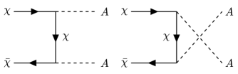
Figure 2: Dark matter annihilation channels.

V Gravitational waves from
  phase transitions

As discussed in Sec. III, when the temperature becomes sufficiently low, patches of the Universe start undergoing a first order phase transition from the false vacuum at the origin to either of the true vacua: $(\phi_{1},\phi_{2})_{\rm true1}$ or $(\phi_{1},-\phi_{2})_{\rm true2}$. When the $\mathcal{Z}_{2}$ breaking parameters are small, the expected gravitational wave signal from a transition to any of those two vacua is similar. For concreteness, in the subsequent analysis we focus on the transition to $(\phi_{1},\phi_{2})_{\rm true1}$.

During such a first order phase transition, bubbles of true vacuum are nucleated and gravitational waves are generated through bubble wall collisions, sound shock waves in the plasma, and magnetohydrodynamic turbulence. The phase transition starts when the bubble nucleation rate becomes comparable to the Hubble expansion rate, i.e., when $\Gamma(T_{*})\sim H^{4}(T_{*})$. The temperature at which this happens is called the nucleation temperature $T_{*}$. The rate for bubble nucleation can be calculated as Linde (1983)

$$\Gamma(T)\approx\left(\frac{S_{E}(T)}{2\pi T}\right)^{\frac{3}{2}}T^{4}\exp\!\left({-\frac{S_{E}(T)}{T}}\right)\ ,$$ (31)

where $S_{E}(T)$ is the Euclidean action dependent on the shape of the effective potential. Denoting $\vec{\phi}=(\phi_{1},\phi_{2})^{T}$, in the case of thermal tunneling $S_{E}(T)$ is given by the integral

$$S_{E}(T)=\int d^{3}x\left[\frac{1}{2}\left(\partial_{\mu}\vec{\phi}\right)^{2}+V_{\rm eff}(\vec{\phi},T)\right],$$ (32)

in which $\vec{\phi}$, assuming spherical symmetry, satisfies the bubble equation of motion,

$$\frac{d^{2}\vec{\phi}}{dr^{2}}+\frac{2}{r}\frac{d\vec{\phi}}{dr}-\vec{\nabla}V_{\rm eff}(\vec{\phi},T)=0\ ,$$ (33)

with the boundary conditions

$$\frac{d\vec{\phi}}{dr}\bigg{|}_{r=0}=0\ ,\ \ \ \ \ \vec{\phi}(\infty)=\vec{\phi}_{\rm false}\ .$$ (34)

Using Eq. (31), the condition for the onset of a phase transition can be written explicitly as

$$\frac{S_{E}(T_{*})}{T_{*}}\approx 4\log\left(\frac{M_{\rm P}}{T_{*}}\right)-\log\left[\left(\frac{4\pi^{3}g_{*}}{45}\right)^{\!\!2}\!\left(\frac{2\pi\,T_{*}}{S_{E}(T_{*})}\right)^{\!\!\frac{3}{2}}\right],$$

where $M_{\rm P}=1.22\times 10^{19}\ {\rm GeV}$ is the Planck mass and $g_{*}$ is the number of degrees of freedom at the temperature $T_{*}$. Equation (V) serves as the source for determining $T_{*}$ for a given set of parameters in the effective potential.

The expected gravitational wave spectrum is fully described by four quantities: bubble wall velocity, nucleation temperature, strength of the phase transition, and its duration. Out of those parameters, only the bubble wall velocity is independent of the shape of the effective potential and we set it to the speed of light, i.e., $v_{w}=c$. Detailed discussions of how to model $v_{w}$ more precisely are provided in Espinosa et al. (2010); Caprini et al. (2016).

The strength of the phase transition is given by the ratio of the energy density of the false vacuum (with respect to the true vacuum) and the energy density of radiation at nucleation temperature,

$$\alpha=\frac{\rho_{\rm vac}(T_{*})}{\rho_{\rm rad}(T_{*})}\ ,$$ (36)

where

$$\rho_{\rm vac}(T) = V_{\rm eff}(\vec{\phi}_{\rm false},T)-V_{\rm eff}(\vec{\phi}_{\rm true},T)$$ (37)

$$- T\frac{\partial}{\partial T}{\left[V_{\rm eff}(\vec{\phi}_{\rm false},T)-V_{\rm eff}(\vec{\phi}_{\rm true},T)\right]}\ \ \ \ \ \$$

and

$$\rho_{\rm rad}(T)=\frac{\pi^{2}}{30}g_{*}T^{4}\ .$$ (38)

The inverse of the duration of the phase transition $\tilde{\beta}$ is

$$\tilde{\beta}=T_{*}\frac{d}{dT}\!\left[\frac{S_{E}(T)}{T}\right]\bigg{|}_{T=T_{*}}\ .$$ (39)

Numerical simulations have been used to derive empirical formulas describing how the expected gravitational wave spectrum from bubble collisions, sound waves, and turbulence depends on the four parameters $v_{w}$, $T_{*}$, $\alpha$, and $\tilde{\beta}$.

The contribution from sound waves is given by Hindmarsh et al. (2014); Caprini et al. (2016)

$$h^{2}\Omega_{s}(f)\, \approx \,\frac{1.9\times 10^{-5}}{\tilde{\beta}}\frac{(f/f_{s})^{3}}{\big{[}1+0.75(f/f_{s})^{2}\big{]}^{7/2}}\left(\frac{g_{*}}{100}\right)^{-\frac{1}{3}}$$ (40)

$$\times \left[\frac{\alpha^{2}}{(1+\alpha)(0.73+0.083\sqrt{\alpha}+\alpha)}\right]^{2}\Upsilon\ ,$$

where the formula for the fraction of the latent heat transformed into the plasma’s bulk motion derived in Espinosa et al. (2010) was used, the peak frequency is

$$f_{s} = (0.19\ {\rm Hz})\left(\frac{T_{*}}{1\ {\rm PeV}}\right)\left(\frac{g_{*}}{100}\right)^{\frac{1}{6}}\tilde{\beta}\ ,\ \ \ \ \ \ \$$ (41)

and $\Upsilon$ is the suppression factor Ellis et al. (2020b) for which we adopt the most recent estimate Guo et al. (2021),

$$\Upsilon=1-\frac{1}{\sqrt{1+\frac{8\pi^{1/3}}{\sqrt{3}\,\tilde{\beta}}\Big{(}\frac{\sqrt{(1+\alpha)(0.73+0.083\sqrt{\alpha}+\alpha)}}{\alpha}\Big{)}}}\ .\ \ \ \ \$$ (42)

The contribution to the gravitational wave spectrum from bubble wall collisions can be written as Kosowsky et al. (1992); Huber and Konstandin (2008); Caprini et al. (2016)

$$h^{2}\Omega_{c}(f)\, \approx \,\frac{2.5\times 10^{-6}}{\tilde{\beta}^{2}}\frac{(f/f_{c})^{2.8}}{1+2.8(f/f_{c})^{3.8}}\left(\frac{g_{*}}{100}\right)^{-\frac{1}{3}}$$ (43)

$$\times \left[\frac{\alpha^{2}+0.25\,\alpha\sqrt{\alpha}}{(1+\alpha)(1+0.72\,\alpha)}\right]^{2},\ \ \ \ \ \$$

where the fraction of the latent heat deposited into the bubble front was adopted from Kamionkowski et al. (1994), and the peak frequency is

$$f_{c} = (0.037\ {\rm Hz})\left(\frac{T_{*}}{1\ {\rm PeV}}\right)\left(\frac{g_{*}}{100}\right)^{\frac{1}{6}}\tilde{\beta}\ .\ \ \ \ \ \$$ (44)

Although turbulence provides a subleading contribution to the signal in the peak region, for completeness we provide the corresponding formula Caprini and Durrer (2006); Caprini et al. (2009),

$$h^{2}\Omega_{t}(f)\, \approx \,\frac{3.4\times 10^{-4}}{\tilde{\beta}}\frac{\epsilon^{2}\ ({f}/{f_{t}})^{3}}{\big{(}1+{8\pi f}/{f_{*}}\big{)}\big{(}1+{f}/{f_{t}}\big{)}^{{11}/{3}}}$$ (45)

$$\times \left(\frac{g_{*}}{100}\right)^{-\frac{1}{3}}\left[\frac{\alpha^{2}}{(1+\alpha)(0.73+0.083\sqrt{\alpha}+\alpha)}\right]^{3/2}\!\!\!\!\!\!,$$

again assuming the fraction of the latent heat transformed into the plasma’s bulk motion from Espinosa et al. (2010). In the above formula the parameter $\epsilon=0.05$ Caprini et al. (2016), the peak frequency

$$f_{t} = (0.27\ {\rm Hz})\,\frac{\tilde{\beta}}{v_{w}}\,\left(\frac{g_{*}}{100}\right)^{\frac{1}{6}}\left(\frac{T_{*}}{1\ {\rm PeV}}\right)\ ,$$ (46)

and the parameter $f_{*}$ Caprini et al. (2016),

$$f_{*}=(0.17\ {\rm Hz})\left(\frac{g_{*}}{100}\right)^{\frac{1}{6}}\left(\frac{T_{*}}{1\ {\rm PeV}}\right)\ .$$ (47)

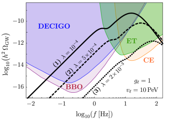
Figure 3: Gravitational wave signatures of the ${\rm SU}(2)_{\ell}$ model for the vev $v_{\ell}=10\,\rm PeV$, gauge coupling $g_{\ell}=1$, and several values of the quartic coupling: $\lambda=\{10^{-4}$, $5\!\times\!10^{-4}$, $2\!\times\!10^{-3}\}$, as described in the figure. Sensitivities of future gravitational wave detectors are also shown: Einstein Telescope Sathyaprakash et al. (2012) (green), Cosmic Explorer Reitze et al. (2019) (orange), DECIGO Yagi and Seto (2011) (blue), and Big Bang Observer Yagi and Seto (2011) (purple). The phase transition parameters corresponding to the curves $(1)$, $(2)$ and $(3)$ are provided in Table 1.

	Lagrangian parameters			Signal parameters
​Curve​	$v_{\ell}$	$\lambda$	$g_{\ell}$	$\alpha$	$\tilde{\beta}$	$T_{*}$
$(1)$	$10\ {\rm PeV}$	$10^{-4}$	$1.0$	2.0	70	$1.2\ {\rm PeV}$
$(2)$	$10\ {\rm PeV}$	$5\times 10^{-4}\!$	$1.0$	0.8	110	$1.5\ {\rm PeV}$
$(3)$	$10\ {\rm PeV}$	$2\times 10^{-3}\!$	$1.0$	0.2	200	$2.0\ {\rm PeV}$

Table 1: Values of the phase transition parameters $\alpha$, $\tilde{\beta}$ and $T_{*}$ for the three benchmark gravitational wave signatures shown in Fig. 3.

To determine the gravitational wave spectra of the ${\rm SU}(2)_{\ell}$ model, we used the software anybubble Masoumi et al. (2017) to compute the Euclidean action $S_{E}$ as a function of temperature for various parameter choices in the effective potential given by Eq. (13). For simplicity, in our analysis we set the quartic couplings to be equal, $\lambda_{1}=\lambda_{2}\equiv\lambda$, and we assumed the same for the vevs, $v_{1}=v_{2}$. As mentioned earlier, we took $|\mu_{12}^{2}|$ and $|\lambda_{7}|$ to be small. Under those assumptions, the effective potential is fully described just by the four parameters $(v_{\ell},\lambda,g_{\ell},T)$. We then numerically determined the nucleation temperature $T_{*}$ for each case via Eq. (V), and calculated the parameters $\alpha$ and $\tilde{\beta}$ using Eqs. (36) and (39), to finally arrive at the expected gravitational wave signal,

$$h^{2}\Omega_{\rm GW}(f)=h^{2}\Omega_{s}(f)+h^{2}\Omega_{c}(f)+h^{2}\Omega_{t}(f)\ ,$$ (48)

using the expressions in Eqs. (40)–(47).

The resulting gravitational wave signatures, for the three representative sets of parameters listed in Table 1, are shown in Fig. 3. In all cases the leading contribution around the peak region comes from sound waves and is given by Eq. (40). The smaller bump towards lower frequencies reflects the bubble collision contribution from Eq. (43). The position of the peak of each signal is proportional to the nucleation temperature, thus signatures corresponding to phase transitions happening at energies higher than $10\ {\rm PeV}$ would be shifted towards higher frequencies. The peak frequency also has a linear dependence on the parameter $\tilde{\beta}$. The height of the signal peak is determined by both $\alpha$ and $\tilde{\beta}$: for larger $\alpha$ the signal is stronger, whereas for larger $\tilde{\beta}$ the signal is weaker.

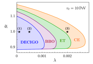
Figure 4: Regions of parameter space $(\lambda,g_{\ell})$ of the ${\rm SU}(2)_{\ell}$ model for $v_{\ell}=10\,{\rm PeV}$ corresponding to a signal detectable, upon one year of data collecting, with a signal-to-noise ratio of at least five, in the experiments: DECIGO (blue), Big Bang Observer (blue and purple), Einstein Telescope (blue, purple and green), Cosmic Explorer (entire shaded region). The stars denote the benchmark parameters in Fig. 3.

Depending on the parameter values, the signal of the model with a symmetry breaking scale $v_{\ell}\sim{\mathcal{O}}(1\!-\!1000)\,{\rm PeV}$ can fall within the sensitivity range of four planned gravitational wave experiments: Einstein Telescope, Cosmic Explorer,DECIGO and Big Bang Observer. The largest signal strength corresponds to a small quartic coupling $\lambda$. In this limit the tree-level term in the effective potential becomes small, and the shape of $V_{\rm eff}$ is determined by the one-loop Coleman-Weinberg term and finite temperature effects. This is known as the supercooling regime Delle Rose et al. (2020); Ellis et al. (2020a); Kawana (2022), characterized by a small $\tilde{\beta}$ and large $\alpha$, which leads to an enhanced gravitational wave signal. For some particle physics models, this scenario can already be searched for in the existing LVK data Badger et al. (2022).

To assess how likely it is for phase transitions in the model to produce a detectable gravitational wave signal, we performed a scan over the parameters $(\lambda,g_{\ell})$ for the vev fixed at $v_{\ell}=10\ {\rm PeV}$, and determined the regions corresponding to a signal-to-noise ratio of at least five after a single year of data collecting with the Einstein Telescope, Cosmic Explorer, DECIGO and Big Bang Observer. The results of the scan are shown in Fig. 4. A large portion of the ${\rm SU}(2)_{\ell}$ model parameter space leading to a first order phase transition will be probed by those experiments, with DECIGO and Big Bang Observer being able to probe also lower symmetry breaking scales.

Finally, as discussed in Sec. III, the model predicts also a gravitational wave signal from domain walls. Indeed, following the analysis of Sec. IV, a successful mechanism for baryogenesis favors a small $\mathcal{Z}_{2}$ breaking parameter $\mu_{12}^{2}$, which leads to a near-degeneracy between the vacua $(\phi_{1},\phi_{2})_{\rm true1}$ and $(\phi_{1},-\phi_{2})_{\rm true2}$ , resulting in the production of domain walls in the early Universe. Their subsequent annihilation gives rise to a gravitational wave background of a predictable shape Saikawa (2017). Nevertheless, given the relation in Eq. (29), the parameter $\mu_{12}^{2}$ cannot be smaller than $(1\,\rm GeV)^{2}$, which implies a considerable suppression of the expected gravitational wave signal for $v_{\ell}\sim 10\ {\rm PeV}$ in this model, making it very unlikely to detect such a domain wall signature in any near-future experiment.

VI Conclusions

Gravitational wave experiments opened an entirely new window of opportunities for probing particle physics models via searches for signatures of first order phase transitions, cosmic strings, and domain walls. Already at this point, the sensitivity of the LVK detectors grants access to regions of parameter space far beyond the reach of any conventional high energy physics experiment. With new gravitational wave experiments planned for construction in the near future, sensitive to a much wider range of frequencies, as well as the upcoming improvements to the existing LVK detectors, the search for physics beyond the Standard Model will certainly intensify and become even more exciting.

In this work we demonstrated how to exploit the upcoming gravitational wave experiments: Einstein Telescope, Cosmic Explorer, DECIGO, and Big Bang Observer, to search for signatures of models explaining simultaneously two of the most pressing open questions in particle physics – the nature of dark matter and the overwhelming domination of matter over antimatter in the present Universe. The solution to the second puzzle requires a period of an out-of-equilibrium dynamics in the early Universe. This can be realized by a first order phase transition, which is precisely the process whose signatures gravitational wave detectors are sensitive to. This shows the increasing importance of gravitational wave experiments for this branch of particle physics in the years to come.

We focused on a representative model of asymmetric dark matter, in which the Standard Model symmetry is extended by a gauged ${\rm SU}(2)_{\ell}$. In this theory, the baryon number excess is generated through a novel type of instanton interactions. With the symmetry breaking scale for the new gauge group at $\sim\mathcal{O}(1\!-\!1000)\ {\rm PeV}$, this model does not alter the Standard Model predictions in collider experiments. Nevertheless, as we have shown, such a high symmetry breaking scale makes it an ideal candidate for gravitational wave searches, with a potential of finding its signatures in all four aforementioned near-future experiments.

A natural continuation of this project would be to consider theories of asymmetric dark matter based on other gauge extensions of the Standard Model, and to develop strategies to differentiate between their gravitational wave signatures. Some examples of such models include a theory based on an ${\rm SU}(4)$ gauge group unifying color and gauged baryon number Fornal et al. (2015), or a theory based on ${\rm SU}(5)$ where color is unified with a dark ${\rm SU}(2)_{D}$ Murgui and Zurek (2022). One could also investigate other asymmetric dark matter theories with extra ${\rm U}(1)$ gauge groups Shelton and Zurek (2010); von Harling et al. (2012), for which an additional cosmic string contribution would be present in the gravitational wave spectrum.

Acknowledgments

We are grateful to the Physical Review D referee for very constructive comments regarding the manuscript. This research was supported by the National Science Foundationunder Grant No. PHY-2213144.

References

- Glashow (1961) S. L. Glashow, Partial Symmetries of Weak Interactions, Nucl. Phys. 22, 579–588 (1961).
- Higgs (1964) P. W. Higgs, Broken Symmetries and the Masses of Gauge Bosons, Phys. Rev. Lett. 13, 508–509 (1964).
- Englert and Brout (1964) F. Englert and R. Brout, Broken Symmetry and the Mass of Gauge Vector Mesons, Phys. Rev. Lett. 13, 321–323 (1964).
- Weinberg (1967) S. Weinberg, A Model of Leptons, Phys. Rev. Lett. 19, 1264–1266 (1967).
- Salam (1968) A. Salam, Weak and Electromagnetic Interactions, 8th Nobel Symposium Lerum, Sweden, May 19-25, 1968, Conf. Proc. C 680519, 367–377 (1968).
- Fritzsch et al. (1973) H. Fritzsch, M. Gell-Mann, and H. Leutwyler, Advantages of the Color Octet Gluon Picture, Phys. Lett. B 47, 365–368 (1973).
- Gross and Wilczek (1973) D.J. Gross and F. Wilczek, Ultraviolet Behavior of Nonabelian Gauge Theories, Phys. Rev. Lett. 30, 1343–1346 (1973).
- Politzer (1973) H. D. Politzer, Reliable Perturbative Results for Strong Interactions? Phys. Rev. Lett. 30, 1346–1349 (1973).
- Chatrchyan et al. (2012) S. Chatrchyan et al. (CMS), Observation of a New Boson at a Mass of 125 GeV with the CMS Experiment at the LHC, Phys. Lett. B 716, 30–61 (2012), arXiv:1207.7235 [hep-ex] .
- Zwicky (1933) F. Zwicky, Die Rotverschiebung von Extragalaktischen Nebeln, Helvetica Physica Acta 6, 110–127 (1933).
- (11) H. Andernach and F. Zwicky, English and Spanish Translation of Zwicky’s (1933) The Redshift of Extragalactic Nebulae, arXiv:1711.01693 [astro-ph.IM] .
- Rubin and Ford (1970) V. C. Rubin and Jr. Ford, W. K., Rotation of the Andromeda Nebula from a Spectroscopic Survey of Emission Regions, Astrophys. J. 159, 379 (1970).
- de Bernardis et al. (2000) P. de Bernardis et al. (Boomerang), A Flat Universe from High Resolution Maps of the Cosmic Microwave Background Radiation, Nature 404, 955–959 (2000), arXiv:astro-ph/0004404 .
- Gavazzi et al. (2007) R. Gavazzi, T. Treu, J. D. Rhodes, L. V. Koopmans, A. S. Bolton, S. Burles, R. Massey, and L. A. Moustakas, The Sloan Lens ACS Survey. 4. The Mass Density Profile of Early-Type Galaxies out to 100 Effective Radii, Astrophys. J. 667, 176–190 (2007), arXiv:astro-ph/0701589 .
- Bai et al. (2019) Y. Bai, A. J. Long, and S. Lu, Dark Quark Nuggets, Phys. Rev. D 99, 055047 (2019), arXiv:1810.04360 [hep-ph] .
- Carr et al. (2010) B. J. Carr, K. Kohri, Y. Sendouda, and J. Yokoyama, New Cosmological Constraints on Primordial Black Holes, Phys. Rev. D 81, 104019 (2010), arXiv:0912.5297 [astro-ph.CO] .
- Bird et al. (2016) S. Bird, I. Cholis, J. B. Munoz, Y. Ali-Haimoud, M. Kamionkowski, E. D. Kovetz, A. Raccanelli, and A. G. Riess, Did LIGO Detect Dark Matter? Phys. Rev. Lett. 116, 201301 (2016), arXiv:1603.00464 [astro-ph.CO] .
- Press et al. (1990) W. H. Press, B. S. Ryden, and D. N. Spergel, Single Mechanism for Generating Large Scale Structure and Providing Dark Missing Matter, Phys. Rev. Lett. 64, 1084 (1990).
- Hui et al. (2017) L. Hui, J. P. Ostriker, S. Tremaine, and E. Witten, Ultralight Scalars as Cosmological Dark Matter, Phys. Rev. D 95, 043541 (2017), arXiv:1610.08297 [astro-ph.CO] .
- Steigman and Turner (1985) G. Steigman and M. S. Turner, Cosmological Constraints on the Properties of Weakly Interacting Massive Particles, Nucl. Phys. B 253, 375–386 (1985).
- Kolb et al. (1999) E. W. Kolb, D. J. H. Chung, and A. Riotto, WIMPzillas! AIP Conf. Proc. 484, 91–105 (1999), arXiv:hep-ph/9810361 .
- Meissner and Nicolai (2019) K. A. Meissner and H. Nicolai, Planck Mass Charged Gravitino Dark Matter, Phys. Rev. D 100, 035001 (2019), arXiv:1809.01441 [hep-ph] .
- Feng (2010) J. L. Feng, Dark Matter Candidates from Particle Physics and Methods of Detection, Ann. Rev. Astron. Astrophys. 48, 495–545 (2010), arXiv:1003.0904 [astro-ph.CO] .
- Sakharov (1967) A. D. Sakharov, Violation of CP Invariance, C Asymmetry, and Baryon Asymmetry of the Universe, Pisma Zh. Eksp. Teor. Fiz. 5, 32–35 (1967).
- Nussinov (1985) S. Nussinov, Technocosmology? Could a Technibaryon Excess Provide a “Natural” Missing Mass Candidate? Phys. Lett. B 165, 55–58 (1985).
- Kaplan (1992) D. B. Kaplan, A Single Explanation for Both the Baryon and Dark Matter Densities, Phys. Rev. Lett. 68, 741–743 (1992).
- Hooper et al. (2005) D. Hooper, J. March-Russell, and Stephen M. West, Asymmetric Sneutrino Dark Matter and the Puzzle, Phys. Lett. B 605, 228–236 (2005), arXiv:hep-ph/0410114 .
- Kaplan et al. (2009) D. E. Kaplan, M. A. Luty, and K. M. Zurek, Asymmetric Dark Matter, Phys. Rev. D 79, 115016 (2009), arXiv:0901.4117 [hep-ph] .
- Petraki and Volkas (2013) K. Petraki and R. R. Volkas, Review of Asymmetric Dark Matter, Int. J. Mod. Phys. A 28, 1330028 (2013), arXiv:1305.4939 [hep-ph] .
- Zurek (2014) K. M. Zurek, Asymmetric Dark Matter: Theories, Signatures, and Constraints, Phys. Rept. 537, 91–121 (2014), arXiv:1308.0338 [hep-ph] .
- Abbott et al. (2016) B. P. Abbott et al. (LIGO Scientific, Virgo), Observation of Gravitational Waves from a Binary Black Hole Merger, Phys. Rev. Lett. 116, 061102 (2016), arXiv:1602.03837 [gr-qc] .
- Einstein (1916) A. Einstein, The Foundation of the General Theory of Relativity, Annalen Phys. 49, 769–822 (1916).
- Kosowsky et al. (1992) A. Kosowsky, M. S. Turner, and R. Watkins, Gravitational Radiation from Colliding Vacuum Bubbles, Phys. Rev. D 45, 4514–4535 (1992).
- Turner (1997) M. S. Turner, Detectability of Inflation Produced Gravitational Waves, Phys. Rev. D 55, R435–R439 (1997), arXiv:astro-ph/9607066 .
- Vachaspati and Vilenkin (1985) T. Vachaspati and A. Vilenkin, Gravitational Radiation from Cosmic Strings, Phys. Rev. D 31, 3052 (1985).
- Sakellariadou (1990) M. Sakellariadou, Gravitational Waves Emitted from Infinite Strings, Phys. Rev. D 42, 354–360 (1990), [Erratum: Phys. Rev. D 43, 4150 (1991)].
- Hiramatsu et al. (2010) T. Hiramatsu, M. Kawasaki, and K. Saikawa, Gravitational Waves from Collapsing Domain Walls, JCAP 05, 032 (2010), arXiv:1002.1555 [astro-ph.CO] .
- Amaro-Seoane et al. (2017) P. Amaro-Seoane et al. (LISA), Laser Interferometer Space Antenna, arXiv:1702.00786 [astro-ph.IM] .
- Punturo et al. (2010) M. Punturo et al., The Einstein Telescope: A Third-Generation Gravitational Wave Observatory, Class. Quant. Grav. 27, 194002 (2010).
- Kawamura et al. (2011) S. Kawamura et al., The Japanese Space Gravitational Wave Antenna: DECIGO, Class. Quant. Grav. 28, 094011 (2011).
- Reitze et al. (2019) D. Reitze et al., Cosmic Explorer: The U.S. Contribution to Gravitational-Wave Astronomy beyond LIGO, Bull. Am. Astron. Soc. 51, 035 (2019), arXiv:1907.04833 [astro-ph.IM] .
- Crowder and Cornish (2005) J. Crowder and N. J. Cornish, Beyond LISA: Exploring Future Gravitational Wave Missions, Phys. Rev. D 72, 083005 (2005), arXiv:gr-qc/0506015 .
- Caldwell et al. (2022) R. Caldwell et al., Detection of Early-Universe Gravitational Wave Signatures and Fundamental Physics, Gen. Relativ. Gravit. 54, 156 (2022), arXiv:2203.07972 [gr-qc] .
- Grojean and Servant (2007) C. Grojean and G. Servant, Gravitational Waves from Phase Transitions at the Electroweak Scale and Beyond, Phys. Rev. D 75, 043507 (2007), arXiv:hep-ph/0607107 .
- Vaskonen (2017) V. Vaskonen, Electroweak Baryogenesis and Gravitational Waves from a Real Scalar Singlet, Phys. Rev. D 95, 123515 (2017), arXiv:1611.02073 [hep-ph] .
- Dorsch et al. (2017) G. C. Dorsch, S. J. Huber, T. Konstandin, and J. M. No, A Second Higgs Doublet in the Early Universe: Baryogenesis and Gravitational Waves, JCAP 05, 052 (2017), arXiv:1611.05874 [hep-ph] .
- Bernon et al. (2018) J. Bernon, L. Bian, and Y. Jiang, A New Insight into the Phase Transition in the Early Universe with Two Higgs Doublets, JHEP 05, 151 (2018), arXiv:1712.08430 [hep-ph] .
- Baldes and Servant (2018) I. Baldes and G. Servant, High Scale Electroweak Phase Transition: Baryogenesis & Symmetry Non-Restoration, JHEP 10, 053 (2018), arXiv:1807.08770 [hep-ph] .
- Chala et al. (2018) M. Chala, C. Krause, and G. Nardini, Signals of the Electroweak Phase Transition at Colliders and Gravitational Wave Observatories, JHEP 07, 062 (2018), arXiv:1802.02168 [hep-ph] .
- Alves et al. (2019) A. Alves, T. Ghosh, H.-K. Guo, K. Sinha, and D. Vagie, Collider and Gravitational Wave Complementarity in Exploring the Singlet Extension of the Standard Model, JHEP 04, 052 (2019), arXiv:1812.09333 [hep-ph] .
- Han et al. (2021) X.-F. Han, L. Wang, and Y. Zhang, Dark Matter, Electroweak Phase Transition, and Gravitational Waves in the Type II Two-Higgs-Doublet Model with a Singlet Scalar Field, Phys. Rev. D 103, 035012 (2021), arXiv:2010.03730 [hep-ph] .
- Azatov et al. (2021) A. Azatov, M. Vanvlasselaer, and W. Yin, Dark Matter Production from Relativistic Bubble Walls, JHEP 03, 288 (2021), arXiv:2101.05721 [hep-ph] .
- Benincasa et al. (2022) N. Benincasa, L. Delle Rose, K. Kannike, and L. Marzola, Multistep Phase Transitions and Gravitational Waves in the Inert Doublet Model, JCAP 12, 025 (2022), arXiv:2205.06669 [hep-ph] .
- Brdar et al. (2019) V. Brdar, A. J. Helmboldt, and J. Kubo, Gravitational Waves from First-Order Phase Transitions: LIGO as a Window to Unexplored Seesaw Scales, JCAP 02, 021 (2019), arXiv:1810.12306 [hep-ph] .
- Okada and Seto (2018) N. Okada and O. Seto, Probing the Seesaw Scale with Gravitational Waves, Phys. Rev. D 98, 063532 (2018), arXiv:1807.00336 [hep-ph] .
- Di Bari et al. (2021) P. Di Bari, D. Marfatia, and Y.-L. Zhou, Gravitational Waves from First-Order Phase Transitions in Majoron Models of Neutrino Mass, JHEP 10, 193 (2021), arXiv:2106.00025 [hep-ph] .
- Zhou et al. (2022) R. Zhou, L. Bian, and Y. Du, Electroweak Phase Transition and Gravitational Waves in the Type-II Seesaw Model, JHEP 08, 205 (2022), arXiv:2203.01561 [hep-ph] .
- Baldes (2017) I. Baldes, Gravitational Waves from the Asymmetric-Dark-Matter Generating Phase Transition, JCAP 05, 028 (2017), arXiv:1702.02117 [hep-ph] .
- Hasegawa et al. (2019) T. Hasegawa, N. Okada, and O. Seto, Gravitational Waves from the Minimal Gauged Model, Phys. Rev. D 99, 095039 (2019), arXiv:1904.03020 [hep-ph] .
- Fornal and Shams Es Haghi (2020) B. Fornal and B. Shams Es Haghi, Baryon and Lepton Number Violation from Gravitational Waves, Phys. Rev. D 102, 115037 (2020), arXiv:2008.05111 [hep-ph] .
- Croon et al. (2019) D. Croon, T. E. Gonzalo, and G. White, Gravitational Waves from a Pati-Salam Phase Transition, JHEP 02, 083 (2019), arXiv:1812.02747 [hep-ph] .
- Huang et al. (2020) W.-C. Huang, F. Sannino, and Z.-W. Wang, Gravitational Waves from Pati-Salam Dynamics, Phys. Rev. D 102, 095025 (2020), arXiv:2004.02332 [hep-ph] .
- Okada et al. (2021) N. Okada, O. Seto, and H. Uchida, Gravitational Waves from Breaking of an Extra in Grand Unification, PTEP 2021, 033B01 (2021), arXiv:2006.01406 [hep-ph] .
- Schwaller (2015) P. Schwaller, Gravitational Waves from a Dark Phase Transition, Phys. Rev. Lett. 115, 181101 (2015), arXiv:1504.07263 [hep-ph] .
- Breitbach et al. (2019) M. Breitbach, J. Kopp, E. Madge, T. Opferkuch, and P. Schwaller, Dark, Cold, and Noisy: Constraining Secluded Hidden Sectors with Gravitational Waves, JCAP 07, 007 (2019), arXiv:1811.11175 [hep-ph] .
- Croon et al. (2018) D. Croon, V. Sanz, and G. White, Model Discrimination in Gravitational Wave spectra from Dark Phase Transitions, JHEP 08, 203 (2018), arXiv:1806.02332 [hep-ph] .
- Hall et al. (2020) E. Hall, T. Konstandin, R. McGehee, H. Murayama, and G. Servant, Baryogenesis From a Dark First-Order Phase Transition, JHEP 04, 042 (2020), arXiv:1910.08068 [hep-ph] .
- Ellis et al. (2020a) J. Ellis, M. Lewicki, and V. Vaskonen, Updated Predictions for Gravitational Waves Produced in a Strongly Supercooled Phase Transition, JCAP 11, 020 (2020a), arXiv:2007.15586 [astro-ph.CO] .
- Kawana (2022) K. Kawana, Cosmology of a Supercooled Universe, Phys. Rev. D 105, 103515 (2022), arXiv:2201.00560 [hep-ph] .
- Dev et al. (2019) P. S. B. Dev, F. Ferrer, Y. Zhang, and Y. Zhang, Gravitational Waves from First-Order Phase Transition in a Simple Axion-Like Particle Model, JCAP 11, 006 (2019), arXiv:1905.00891 [hep-ph] .
- Von Harling et al. (2020) B. Von Harling, A. Pomarol, O. Pujolas, and F. Rompineve, Peccei-Quinn Phase Transition at LIGO, JHEP 04, 195 (2020), arXiv:1912.07587 [hep-ph] .
- Delle Rose et al. (2020) L. Delle Rose, G. Panico, M. Redi, and A. Tesi, Gravitational Waves from Supercool Axions, JHEP 04, 025 (2020), arXiv:1912.06139 [hep-ph] .
- Craig et al. (2020) N. Craig, N. Levi, A. Mariotti, and D. Redigolo, Ripples in Spacetime from Broken Supersymmetry, JHEP 21, 184 (2020), arXiv:2011.13949 [hep-ph] .
- Fornal et al. (2021) B. Fornal, B. Shams Es Haghi, J.-H. Yu, and Y. Zhao, Gravitational Waves from Mini-Split SUSY, Phys. Rev. D 104, 115005 (2021), arXiv:2104.00747 [hep-ph] .
- Greljo et al. (2020) A. Greljo, T. Opferkuch, and B. A. Stefanek, Gravitational Imprints of Flavor Hierarchies, Phys. Rev. Lett. 124, 171802 (2020), arXiv:1910.02014 [hep-ph] .
- Fornal (2021) B. Fornal, Gravitational Wave Signatures of Lepton Universality Violation, Phys. Rev. D 103, 015018 (2021), arXiv:2006.08802 [hep-ph] .
- Fornal et al. (2017) B. Fornal, Y. Shirman, T. M. P. Tait, and J. Rittenhouse West, Asymmetric Dark Matter and Baryogenesis from , Phys. Rev. D 96, 035001 (2017), arXiv:1703.00199 [hep-ph] .
- Schwaller et al. (2013) P. Schwaller, T. M. P. Tait, and R. Vega-Morales, Dark Matter and Vectorlike Leptons from Gauged Lepton Number, Phys. Rev. D 88, 035001 (2013), arXiv:1305.1108 [hep-ph] .
- Agnese et al. (2016) R. Agnese et al. (SuperCDMS), New Results from the Search for Low-Mass Weakly Interacting Massive Particles with the CDMS Low Ionization Threshold Experiment, Phys. Rev. Lett. 116, 071301 (2016), arXiv:1509.02448 [astro-ph.CO] .
- Quiros (1999) M. Quiros, Finite Temperature Field Theory and Phase Transitions, in ICTP Summer School in High-Energy Physics and Cosmology (1999) pp. 187–259, arXiv:hep-ph/9901312 .
- Ginzburg and Krawczyk (2005) I. F. Ginzburg and M. Krawczyk, Symmetries of Two Higgs Doublet Model and CP Violation, Phys. Rev. D 72, 115013 (2005), arXiv:hep-ph/0408011 .
- Battye et al. (2011) R. A. Battye, G. D. Brawn, and A. Pilaftsis, Vacuum Topology of the Two Higgs Doublet Model, JHEP 08, 020 (2011), arXiv:1106.3482 [hep-ph] .
- Saikawa (2017) K. Saikawa, A Review of Gravitational Waves from Cosmic Domain Walls, Universe 3, 40 (2017), arXiv:1703.02576 [hep-ph] .
- Dick et al. (2000) K. Dick, M. Lindner, M. Ratz, and D. Wright, Leptogenesis with Dirac Neutrinos, Phys. Rev. Lett. 84, 4039–4042 (2000), arXiv:hep-ph/9907562 .
- Murayama and Pierce (2002) H. Murayama and A. Pierce, Realistic Dirac Leptogenesis, Phys. Rev. Lett. 89, 271601 (2002), arXiv:hep-ph/0206177 .
- Shu et al. (2007) J. Shu, T. M. P. Tait, and C. E. M. Wagner, Baryogenesis from an Earlier Phase Transition, Phys. Rev. D 75, 063510 (2007), arXiv:hep-ph/0610375 .
- Blennow et al. (2011) M. Blennow, B. Dasgupta, E. Fernandez-Martinez, and N. Rius, Aidnogenesis via Leptogenesis and Dark Sphalerons, JHEP 03, 014 (2011), arXiv:1009.3159 [hep-ph] .
- Morrissey et al. (2005) D. E. Morrissey, T. M. P. Tait, and C. E. M. Wagner, Proton Lifetime and Baryon Number Violating Signatures at the CERN LHC in Gauge Extended Models, Phys. Rev. D 72, 095003 (2005), arXiv:hep-ph/0508123 .
- Joyce et al. (1996) M. Joyce, T. Prokopec, and N. Turok, Nonlocal Electroweak Baryogenesis. Part 1: Thin Wall Regime, Phys. Rev. D 53, 2930–2957 (1996), arXiv:hep-ph/9410281 .
- Cohen et al. (1994) A. G. Cohen, D. B. Kaplan, and A. E. Nelson, Diffusion Enhances Spontaneous Electroweak Baryogenesis, Phys. Lett. B 336, 41–47 (1994), arXiv:hep-ph/9406345 .
- Riotto (1996) A. Riotto, Towards a Nonequilibrium Quantum Field Theory Approach to Electroweak Baryogenesis, Phys. Rev. D 53, 5834–5841 (1996), arXiv:hep-ph/9510271 .
- Harvey and Turner (1990) J. A. Harvey and M. S. Turner, Cosmological Baryon and Lepton Number in the Presence of Electroweak Fermion Number Violation, Phys. Rev. D 42, 3344–3349 (1990).
- Workman and Others (2022) R. L. Workman and Others (Particle Data Group), Review of Particle Physics, PTEP 2022, 083C01 (2022).
- Krnjaic (2016) G. Krnjaic, Probing Light Thermal Dark-Matter With a Higgs Portal Mediator, Phys. Rev. D 94, 073009 (2016), arXiv:1512.04119 [hep-ph] .
- Linde (1983) A. D. Linde, Decay of the False Vacuum at Finite Temperature, Nuclear Physics B 216, 421 – 445 (1983).
- Espinosa et al. (2010) J. R. Espinosa, T. Konstandin, J. M. No, and G. Servant, Energy Budget of Cosmological First-Order Phase Transitions, JCAP 06, 028 (2010), arXiv:1004.4187 [hep-ph] .
- Caprini et al. (2016) C. Caprini et al., Science with the Space-Based Interferometer eLISA. II: Gravitational Waves from Cosmological Phase Transitions, JCAP 04, 001 (2016), arXiv:1512.06239 [astro-ph.CO] .
- Hindmarsh et al. (2014) M. Hindmarsh, S. J. Huber, K. Rummukainen, and D. J. Weir, Gravitational Waves from the Sound of a First Order Phase Transition, Phys. Rev. Lett. 112, 041301 (2014), arXiv:1304.2433 [hep-ph] .
- Ellis et al. (2020b) J. Ellis, M. Lewicki, and J. M. No, Gravitational Waves from First-Order Cosmological Phase Transitions: Lifetime of the Sound Wave Source, JCAP 07, 050 (2020b), arXiv:2003.07360 [hep-ph] .
- Guo et al. (2021) H.-K. Guo, K. Sinha, D. Vagie, and G. White, Phase Transitions in an Expanding Universe: Stochastic Gravitational Waves in Standard and Non-Standard Histories, JCAP 01, 001 (2021), arXiv:2007.08537 [hep-ph] .
- Huber and Konstandin (2008) S. J. Huber and T. Konstandin, Gravitational Wave Production by Collisions: More Bubbles, JCAP 09, 022 (2008), arXiv:0806.1828 [hep-ph] .
- Kamionkowski et al. (1994) M. Kamionkowski, A. Kosowsky, and M. S. Turner, Gravitational Radiation from First Order Phase Transitions, Phys. Rev. D 49, 2837–2851 (1994), arXiv:astro-ph/9310044 .
- Caprini and Durrer (2006) C. Caprini and R. Durrer, Gravitational Waves from Stochastic Relativistic Sources: Primordial Turbulence and Magnetic Fields, Phys. Rev. D 74, 063521 (2006), arXiv:astro-ph/0603476 .
- Caprini et al. (2009) C. Caprini, R. Durrer, and G. Servant, The Stochastic Gravitational Wave Background from Turbulence and Magnetic Fields Generated by a First-Order Phase Transition, JCAP 12, 024 (2009), arXiv:0909.0622 [astro-ph.CO] .
- Sathyaprakash et al. (2012) B. Sathyaprakash et al., Scientific Objectives of Einstein Telescope, Class. Quant. Grav. 29, 124013 (2012),[Erratum: Class. Quant. Grav. 30, 079501 (2013)], arXiv:1206.0331 [gr-qc].
- Yagi and Seto (2011) K. Yagi and N. Seto, Detector Configuration of DECIGO/BBO and Identification of Cosmological Neutron-Star Binaries, Phys. Rev. D 83, 044011 (2011), [Erratum: Phys.Rev.D 95, 109901 (2017)], arXiv:1101.3940 [astro-ph.CO] .
- Masoumi et al. (2017) A. Masoumi, K. D. Olum, and B. Shlaer, Efficient Numerical Solution to Vacuum Decay with Many Fields, JCAP 01, 051 (2017), arXiv:1610.06594 [gr-qc] .
- Badger et al. (2022) C. Badger, B. Fornal, K. Martinovic, A. Romero, K. Turbang, H.-K. Guo, A. Mariotti, M. Sakellariadou, A. Sevrin, F.-W. Yang, and Y. Zhao, Probing Early Universe Supercooled Phase Transitions with Gravitational Wave Data, arXiv:2209.14707 [hep-ph] , accepted by Phys. Rev. D .
- Fornal et al. (2015) B. Fornal, A. Rajaraman, and T. M. P. Tait, Baryon Number as the Fourth Color, Phys. Rev. D 92, 055022 (2015), arXiv:1506.06131 [hep-ph] .
- Murgui and Zurek (2022) C. Murgui and K. M. Zurek, Dark Unification: A UV-Complete Theory of Asymmetric Dark Matter, Phys. Rev. D 105, 095002 (2022), arXiv:2112.08374 [hep-ph] .
- Shelton and Zurek (2010) J. Shelton and K. M. Zurek, Darkogenesis: A Baryon Asymmetry from the Dark Matter Sector, Phys. Rev. D 82, 123512 (2010), arXiv:1008.1997 [hep-ph] .
- von Harling et al. (2012) B. von Harling, K. Petraki, and R. R. Volkas, Affleck-Dine Dynamics and the Dark Sector of Pangenesis, JCAP 05, 021 (2012), arXiv:1201.2200 [hep-ph] .