SLAC-PUB-17701 September 2022

Model-Agnostic Exploration of the Mass Reach
of Precision Higgs Boson Coupling Measurements

Michael E. Peskin

SLAC, Stanford University, Menlo Park, California 94025 USA

ABSTRACT

To understand the possibility for precision Higgs boson coupling measurements to access effects of very heavy new particles, I present five scenarios in which significant deviations in Higgs boson couplings are produced by new particles with multi-TeV masses. These scenarios indicate that such precision measurements provide opportunities to reach well beyond the capabilities of direct particle searches at the HL-LHC.

Submitted to the Proceedings of US Community Study
on the Future of Particle Physics (Snowmass 2021)

1 Introduction

One of the goals of a program of precision measurements on the Higgs boson is to prove that the Higgs boson is affected by new physics. Ideally, these precision measurements should indicate the existence of new, undiscovered particles. These precision measurements would be especially powerful if they can be sensitive to new particles that are well beyond the search reach of the High Luminosity Large Hadron Collider (HL-LHC).

Unfortunately, it is not so straightforward to test this claim. Models of Beyond-Standard-Model (BSM) physics typically contain many parameters that can be adjusted. It is always possible to cherry-pick points in parameter space that give very strong sensitivity to particles of high mass. Examples are cited in [1, 2]. But it may not be clear to what extent these points are generic rather than exceptional.

One solution is to restrict oneself to the same subsets of BSM model space that are examined at the LHC. However, this hides an important strength of precision Higgs measurements. In complex BSM models, the studies done by the LHC experiments often rely on particular scenarios that are favorable for direct particle discovery. But a feature of precision measurements is that they often give access to a different class of models than those for which the the lowest-mass BSM particles are light enough to be discovered at the LHC. This complementarity has been noticed in supersymmetry models, in scans of the PMSSM parameter set such as  [3]. However, such multi-parameter scans are reliant on public codes that may not be tested over the whole parameter region of interest. For example, this particular study uses a version of the code HDECAY [4] that is not accurate for very heavy squark masses. In general, it is very difficult to check that public codes for complex models written with low-mass BSM particles in mind are valid uniformly over the whole parameter space.

In this note, I approach this question in a different way. I identify specfic scenarios in which integrating out individual heavy particles or heavy particle sectors leads to potentially large corrections to the Higgs boson couplings. I base my analysis on Standard Model Effective Field Theory (SMEFT). I present the Wilson coefficients generated in SMEFT for the leading corrections to the Standard Model Higgs predictions. These expressions isolate a small number of parameters that are important to each particular scenario. For each case, this leads to a small parameter space that can be explored comprehensively. These scenarios then indicate opportunities for the discovery of new physics up to high mass scales by Higgs boson precision measurements. The scenarios I discuss are simple representations of the physics of more complicated BSM models. In fact, they are deliberately oversimplified to make the specific physics mechanism clear. In each case, this points to a path to find these mechanism working in more complete but more complicated models.

After some general orientation, I will explore the following scenarios: (a) the Strongly Coupled Light Higgs (SILH), (b) two-Higgs-doublet (THDM) models, treated at the tree level; (c) Higgs field mixing with a scalar singlet boson field ; (d) integration out of a heavy vectorlike quark; (e) an effect of the stop-higgsino system that appears in the Minimal Supersymmetric Standard Model.

For each case, I will give a plot of the reach in the mass of the new particles in TeV. Note that I quote 3 $\sigma$ and 5-$\sigma$ discovery reach, not exclusion limits. The projected discovery reach of the HL-LHC improves with time, but it is generally expected that the LHC cannot discover new pair-produced new particles with masses as high as 2 TeV, except in cases with very high cross sections and striking signatures, for example, a gluino pair decaying to 4 heavy flavor jets plus missing energy. For example, in [5], the discovery reach at the HL-LHC for vectorlike quarks is estimated not to exceed 1.5 TeV and the reach for top squarks is estimated to be 1.4 TeV. On the other hand, we will see that precision Higgs boson coupling measurements can be sensitive to these particles at masses well above 2 TeV.

2 General orientation

In SMEFT, the effective Lagrangian describing the Higgs boson and its decays is taken to be

$${\cal L}={\cal L}_{SM}+\sum_{J}{c_{J}\over v^{D_{J}-4}}{\cal O}_{J}$$ (1)

where ${\cal L}_{SM}$ is the Lagrangian of the Standard Model (SM), the ${\cal O}_{J}$ are higher-dimension operators respecting the symmetries of the SM, generated by integrating out heavy fields, and the $c_{J}$ are dimensionless numbers, the Wilson coefficients. I take $v$, the Higgs field vacuum expectation value, to be the reference mass scale for this expansion. The leading corrections to the Higgs boson couplings are given by the operators of dimension $D_{j}=6$. The coefficients of these operators are proportional to $M^{-2}$, where $M$ is the mass of the heavy particles, and so the corrections to the corresponding $c_{j}$ and to the dimensionless Higgs boson couplings are of the order of $v^{2}/M^{2}$.

A naive estimation of the corrections to the Higgs boson couplings might be obtained by setting $M=2$ TeV and putting the coefficient 1 in front of the dimensional estimate. This gives the size of these effects as

tree level effects: $$v^{2}/M^{2}\sim 1\%$$

loop level effects: $$(g^{2}/4\pi)v^{2}/M^{2}\sim 0.1\%$$ (2)

Since the capability of proposed $e^{+}e^{-}$ Higgs factories is to measure the Higgs boson couplings to precisions of order 1%, these estimate suggest that the mass reach of Higgs precision is small.

However, in many cases, the coefficient in front of the parametric dependence can be a large dimensionless number. Those cases give opportunties for the precision measurement of Higgs couplings to be an especially powerful route to discovery. In this paper, I study a few concrete examples of systems that generate such large couplings.

For most of the examples, I will discuss only the corrections to Higgs boson couplings that can be studied at the low-energy stages of $e^{+}e^{-}$ Higgs factories, at center of mass energies close to 250 GeV, 360 GeV, and 500 GeV. I will ignore the dimension 4 and 6 operators involving the top quark field. For definiteness, the plots below will compare the deviations expected in the various scenarios to the the projected errrors in Higgs couplings expected for the 500 GeV International Linear Collider (ILC) [2, 6]. Details of the SMEFT analysis for ILC projections are given in [1, 7]. The measurement of the Higgs self-coupling, which is possible at 500 GeV and above, can add to the evidence for new physics, but that effect will not be included in the plots.

Note that whenever we add dimension-6 operators to the SM Lagrangian, we must also modify the SM parameters, which are fit to data. I do this by shifting the basic parameters $v$, $g$, $g^{\prime}$, $\lambda$ and the quark and lepton Yukawa couplings so that the predicted values of $\alpha(m_{Z})$, $G_{F}$, $m_{Z}$, $m_{h}$, and the fermion masses $m_{f}$ remain unchanged.

3 Strongly Interacting Light Higgs

One set of models that is known to give large coefficients is that in which the Higgs boson is assumed to be a composite particle bound by new strongly interacting forces. A simple framework for the SMEFT Wilson coefficients generated by this hypothesis is the Strongly Interacting Light Higgs (SILH) model, suggested in [8]. This model is characterized by a coupling $g_{*}$, which is assumed to be strong, and a scale $\Lambda$ of resonances associated with the strong interactions. I take $H$ to be the effective Higgs doublet field in the low-energy Lagrangian. Then the $c_{j}$ for dimension-6 operators naturally contain factors $v^{2}/\Lambda^{2}$. The largest contributions come from the operators [16]

$$\Delta{\cal L}={c_{H}\over 2v^{2}}\ (\partial_{\mu}(H^{\dagger}H))^{2}+{c_{b}\over v^{2}}\ |H|^{2}\,Q_{L}\cdot Hb_{R}+h.c.\ ,$$ (3)

for which

$$c_{H}=c_{b}=g_{*}^{2}{v^{2}\over\Lambda^{2}}$$ (4)

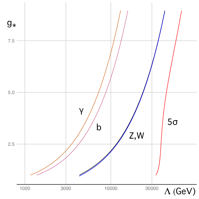
Figure 1: Mass reach for the deviation in the Higgs boson couplings Higgs compositeness, as described by the SILH model. The blue, black, magenta, and chocolate curves indicate the 3 $\sigma$ contours for the deviation in the $HWW$, $HZZ$, $Hgg$, and $H\gamma\gamma$ couplings in a SMEFT fit to projected ILC data up to 500 GeV. The curves are plotted in the $(\Lambda,g_{*})$ plane. The red curves show the 5 $\sigma$ contour for the full SMEFT fit.

In Fig. 1, I plot the contours in the ($\Lambda,g_{*}$) plane along which individual Higgs boson couplings have a 3 $\sigma$ deviation from the SM expectation, assuming measurements with the uncertainties expected for the 500 GeV ILC. Other Higgs factory proposals give very similar expectations. This figure is very similar to Fig. 8.4 of [9], where the limits for the various Higgs factories are displayed separately. The combination of these effects and effects of other dimension-6 SMEFT operators gives the contour for a 5 $\sigma$ deviation from the SM which is also shown in the figure. (Here and below, the distance in $\sigma$ between the new model and the SM is computed as in Sec. 7 of [1].) The significance of the deviations is boosted at small values of $g_{*}$ by contributions from deviations in precision electroweak observables.

4 Two Higgs doublet models

A set of models that gives corrections to the Higgs boson couplings at the tree level is built by adding to the SM a second Higgs doublet. The literature on Two Higgs Doublet models (THDM) is vast. Recently, there has been much interest in the alignment limit [10], in which the mixing has very small effects on the couplings of the 125 GeV Higgs boson while the new bosons remain light enough to observe at the LHC. Here I will consider the decoupling limit [11], where the new bosons are very heavy, perhaps out of reach of the LHC. For simplicity, I include only the leading correction for large masses of the new Higgs bosons. A more complete discussion of this limit has been given in [12, 13].

To make the description of the decoupling limit more transparent, I begin with a description in terms of a light doublet field $h$ and a heavy doublet field $\Phi$. The most general renormalizable Lagrangian for these fields is

$${\cal L} = |D_{\mu}h|^{2}+\mu^{2}|h|^{2}-\lambda|h|^{4}+|D_{\mu}\Phi|^{2}-M^{2}|\Phi|^{2}$$ (5)

$$\hskip 72.26999pt+\eta|h|^{2}(h^{\dagger}\Phi+\Phi^{\dagger}h)+\cdots\ ,$$

with $\mu^{2}\ll M^{2}$. I consider the case $M^{2}>0$, so that the heavy field does not obtain on its own a large $SU(2)\times U(1)$-breaking expectation value. The omitted terms are proportional to $h^{2}\Phi^{2}$ and higher powers of $\Phi$. For the leading $v^{2}/M^{2}$ effect at the tree level, only the terms shown explicitly in (5) are relevant.

The field $h$ acquires a vacuum expectation value $\left\langle{h}\right\rangle=(0,v_{h})/\sqrt{2}$ where $v_{h}$ is very close to the SM expresson $\sqrt{\mu^{2}/\lambda}$. The coupling $\eta$ generates a small mixing between $h$ and $\Phi$ that induces $\left\langle{\Phi}\right\rangle=(0,v_{\Phi})/\sqrt{2}$, where

$$v_{\Phi}=\eta{v_{h}^{2}\over 2M^{2}}\ .$$ (6)

One linear combination of $h$ and $\Phi$ has the vacuum expectation value. This is reflected in the Goldstone boson mass eigenstate

$$\pi^{0}=\pi_{h}^{0}+{\eta v^{2}/2\over M^{2}}\pi^{0}_{\Phi}\ .$$ (7)

On the other hand, the mass eigenstate of the light CP-even boson is

$$H^{0}=h^{0}+{2\mu^{2}+3\eta v^{2}/2\over M^{2}}h^{0}_{\Phi}\ .$$ (8)

The 125 GeV Higgs boson mass $m_{H}^{2}$ equals $2\mu^{2}$ to this order. Then the small angle between these vectors,

$$\gamma={m_{H}^{2}+\eta v^{2}\over M^{2}}\ ,$$ (9)

is directly observable as a deviation of the Higgs boson couplings from the Standard Model expectation $y_{f}=\sqrt{2}m_{f}/v$.

In the THDM at the tree level, the deviation in the Higgs couplings to $W$ and $Z$ is of order $v^{4}/M^{4}$. The $W$ and $Z$ couplings do receive leading contributions in other extended Higgs sections, for example, those discussed in the next section.

In a typical THDM, discrete symmetries force one linear combination of $h$ and $\Phi$ ($\Phi_{1}$) to couple to one set of quarks and leptons, with the orthogonal linear combination $\Phi_{2}$ coupling to a different set of quarks and leptons. For example, in the Type II THDM found in supersymmetric models, $\Phi_{1}$ couples to the down-type quarks and charged leptons while $\Phi_{2}$ couples to the up-type quarks. Define

$$\tan\beta=\left\langle{\Phi_{2}}\right\rangle/\left\langle{\Phi_{1}}\right\rangle\ ,$$ (10)

nd distinguish the two fields by restricting to $\tan\beta>1$. Then the relative corrections to the Higgs couplings for fermions that receive their masses from $\Phi_{1}$ are

$${\Delta y_{f}\over y_{f}}=-\gamma\cdot\tan\beta$$ (11)

while the relative corrections to the Higgs couplings for fermions for fermions that receive their masses from $\Phi_{2}$ are

$${\Delta y_{f}\over y_{f}}=\gamma/\tan\beta\ .$$ (12)

In supersymmetric models, the value of $\eta$ is typically small. For example, the contribution to $\eta$ from the $SU(2)$ D-term is

$$-{g^{2}\over 8}\,\sin 2\beta\,\cos 2\beta\to 0.1/\tan\beta$$ (13)

in the large $\tan\beta$ limit. In more general THDMs, $\eta$ can be larger, up to $\eta\sim 1$.

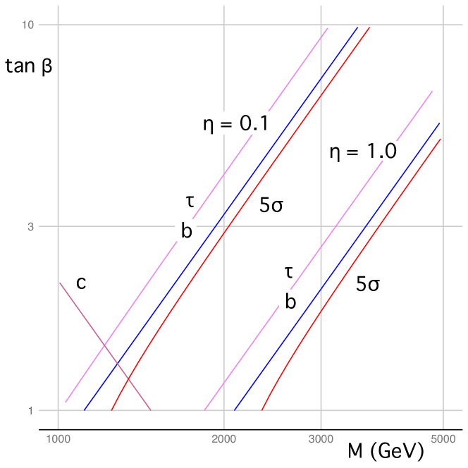
Figure 2: Mass reach for the deviation in the Higgs boson couplings due to the mixing of the Higgs boson with a second Higgs doublet. The blu and magenta curves indicate the 3 $\sigma$ contours for the deviation in the $Hbb$, $H\tau\tau$ couplings in a SMEFT fit to projected ILC data up to 500 GeV. The curves are plotted in the $(M,\tan\beta)$ plane for $\eta=0.1$ (left curves) and $\eta=1.0$ (right curves). The red curves show the 5 $\sigma$ contour for the full SMEFT fit.

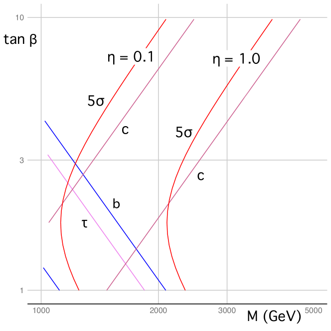
Figure 3: Mass reach for the deviation in the Higgs boson couplings due to the mixing of the Higgs boson with a second Higgs doublet. The blue, magenta, and pink curves indicate the 3 $\sigma$ contours for the deviation in the $Hbb$, $H\tau\tau$, and $Hcc$ couplings in a SMEFT fit to projected ILC data up to 500 GeV. The curves are plotted in the $(M,\tan\beta)$ plane for $\eta=0.1$ (left curves) and $\eta=1.0$ (right curves). The red curves show the 5 $\sigma$ contour for the full SMEFT fit.

In Figs. 2 and 3, I plot the contours in the ($M,\tan\beta$) plane along which individual Higgs boson couplings have a 3 $\sigma$ deviation from the Standard Model expectation, assuming measurements with the uncertainties expected for the 500 GeV ILC. The combination of these effects and other effects of dimension-6 operators gives the contour for a 5 $\sigma$ deviation from the Standard Model which is also shown in the figure. Figure 2 shows the reach for the standard Type II model in which the Yukawa couplings of the $b$ and $\tau$ are enhanced by $\tan\beta$. In complete supersymmetric models, the expected mass reach at the HL-LHC for the heavy Higgs boson is below 1 TeV for low values of $\tan\beta$ [14], leading to a parameter region where the precision Higgs reach extends beyond this. That region is broader for models with larger values of $\eta$. Figure 3 shows the corresponding situation for a flavorful THDM in which the Higgs coupling to charm is enhanced by $\tan\beta$.

5 Higgs field mixing with a singlet scalar field

It is also possible to add to the Standard Model a heavy singlet Higgs field coupling to the 125 GeV Higgs boson through

$${\cal L} = |D_{\mu}h|^{2}+\mu^{2}|h|^{2}-\lambda|h|^{4}+|D_{\mu}\Phi|^{2}-M^{2}|\Phi|^{2}-{\mu_{\Phi}\over 3!}\Phi^{3}-{\lambda_{\Phi}\over 4!}\Phi^{4}$$ (14)

$$\hskip 14.45377pt-\ A|h|^{2}\Phi-k|h|^{2}\Phi^{2}+\cdots\ .$$

Note that $A$ has the dimensions of GeV; I will treat $A/M$ as being order 1. Such a field can substantially modify the Higgs potential, leading to the possibility of a first-order electroweak phase transition, while maintaining smaller effects on the Higgs boson couplings to fermions and vector bosons. In (14), the cubic $A$ term gives the dominant effect. This is a mixing of the singlet Higgs field into the 125 GeV Higgs boson with mixing angle

$$\gamma={Av\over M^{2}}.$$ (15)

For $A\sim M$, $v\ll M$, this effect appears as a uniform decrease in Higgs boson couplings by the factor

$$\cos\gamma\sim 1-\frac{1}{2}\gamma^{2}\sim 1-\frac{1}{2}{A^{2}v^{2}\over M^{4}}\ .$$ (16)

In models with a $Z_{2}$ symmetry that forbids this term, substantial reach for effects of the singlet field can still be obtained through loop effects; see  [15].

The largest effects of the Higgs-singlet mixing are seen in the self-coupling and in $c_{H}$ [16],

$$c_{H}={A^{2}v^{2}\over M^{4}}\qquad c_{6}=-{kA^{2}v^{2}\over 2\lambda M^{4}}-{\mu_{\Phi}A^{3}v^{2}\over 3!\,\lambda M^{6}}$$ (17)

Again, note that both expressions are of order $1/M^{2}$. It is important that $c_{H}$ modifies all Higgs boson couplings equally, so its effects can only be seen by measurements sensitive to the absolute normalization of Higgs couplings.

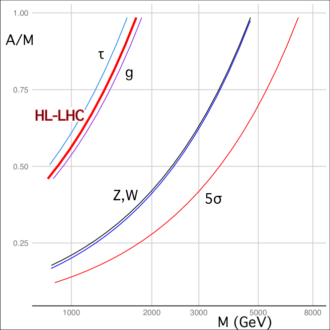
Figure 4: Mass reach for the deviation in the Higgs boson couplings due Higgs mixing with a heavy scalar singlet. The blue, black, violet, and light blue curves indicate, respectively, the 3 $\sigma$ contours for the deviation in the $HWW$, $HZZ$, $Hgg$, and $H\tau\tau$ couplings in a SMEFT fit to projected ILC data up to 500 GeV. The curves are plotted in the $(M,A/M)$ plane. The red curve shows the 5 $\sigma$ contour for the full SMEFT fit. The heavy red line shows the 5 $\sigma$ contour that would be obtained from an HL-LHC 1 sigma uncertainty of 3% on the overall signal strength for Higgs processes.

In Fig. 4, I plot the contours in the ($M,A/M$) plane along which individual Higgs boson couplings have a 3 $\sigma$ deviation from the Standard Model expectation, assuming measurements with the uncertainties expected for the 500 GeV ILC. The combination of these effects and others gives the contour for a 5 $\sigma$ deviation from the Standard Model which is also shown in the figure. For comparison, the heavy red line gives the 5 $\sigma$ contour corresponding to a 3% uncertainty in the overall signal strength for Higgs reactions that might optimistically be measured at the HL-LHC. This corresponds to a 1.5% uncertainty in the scale of Higgs boson couplings. Of course, the LHC determination has more model-dependence than that obtained from $e^{+}e^{-}$ Higgs factories.

It should be noted that there is search reach at the HL-LHC for singlet Higgs bosons up to a mass of 2.5 TeV, but only in models with very large and visible Higgs-singlet mixing; see, for example, Fig. 54 of [17]. The relevant parameter region is above the top of the plot in Fig. 4.

The effect on the Higgs self-coupling is larger than that shown here by a factor

$$1/\lambda\sim{\cal O}(10)\ .$$ (18)

That is, few-percent-level changes in the $HWW$ and $HZZ$ couplings can potentially signal order-1 changes in the Higgs self-coupling, though there might be compensating factors. The relation between the deviations in Higgs couplings to $W$ and $Z$ and those in the self-coupling are studied in explicit models in [18, 19, 20]. Note that I do not include the effect of a deviation in the Higgs self-coupling in the discovery significance plotted in Fig. 4.

6 Models with vectorlike quarks

Integration out of heavy new particles leads to loop corrections to the Higgs boson couplings. These are naturally of the order of

$${g^{2}\over 4\pi}\ {v^{2}\over M^{2}}$$ (19)

and often are at the parts-per-mil level. However, there are exceptions. These occur when the loops acquire large factors from coupling constants, combinatoric factors, factors of $\tan\beta$, or large mass ratios.

The simplest context in which this occurs is the integration out of a doublet of heavy vectorlike quarks. I consider the multiplet (Q, U, D), where $Q$ is an $SU(2)$ doublet and $U$ and $D$ are $SU(2)$ singlets with hypercharges $2/3$ and $-1/3$. The Lagrangian is

$${\cal L} = \overline{Q}(\not{\hbox{\kern-4.0pt$D$}}-M)Q+\overline{U}(\not{\hbox{\kern-4.0pt$D$}}-M)U+\overline{D}(\not{\hbox{\kern-4.0pt$D$}}-M)D$$ (20)

$$= \hskip 7.22743pt+(y_{D}\overline{Q}\cdot H\,D+y_{U}\overline{Q}\cdot\widetilde{H}\,U+h.c.)$$

where $\widetilde{H}_{a}=\epsilon_{ab}H^{*}_{b}$. For simplicity, I have taken the masses of the heavy quarks to be equal. I ignore the couplings of this doublet to light quarks, which must be treated model by model.

The largest contributions in this case come from the operators [21]

$$\Delta{\cal L}={c_{H}\over 2v^{2}}\ (\partial_{\mu}(H^{\dagger}H))^{2}+{g_{s}c_{GG}\over v^{2}}\ |H|^{2}G^{a}_{\mu\nu}G^{a\mu\nu}\ ,$$ (21)

where $g_{s}$ is the QCD coupling constant, for which

$$c_{H}={3\over(4\pi)^{2}}{4v^{2}\over 5M^{2}}(y_{U}^{2}+y_{D}^{2})^{2}\ ,\qquad c_{GG}=-{1\over(4\pi)^{2}}{v^{2}\over 3M^{2}}(y_{U}^{2}+y_{D}^{2})\ .$$ (22)

These are small effects if the Yukawa couplings $y_{U}$ and $y_{D}$ are small, but there is no reason for this. In Little Higgs models, for example, the top quark Yukawa coupling is given by

$$y_{t}^{2}\approx 1={y_{1}^{2}y_{2}^{2}\over y_{1}^{2}+y_{2}^{2}}\ ,$$ (23)

forcing both underlying Yukawa couplings to be greater than 1. Even a value $y_{U}=3$ still corresponds to $\alpha_{U}=0.7$ and give relatively small shifts of TeV-scale vectorlike quark masses. It is true that the calculation of $c_{GG}$ in Little Higgs models typically leads to cancellations due to the extra symmetries of the Little Higgs mechanism. To see how this works in explicit models, see [22, 23, 24]. These models do still give a search reach beyond the HL-LHC value of 1.5 TeV quoted above.

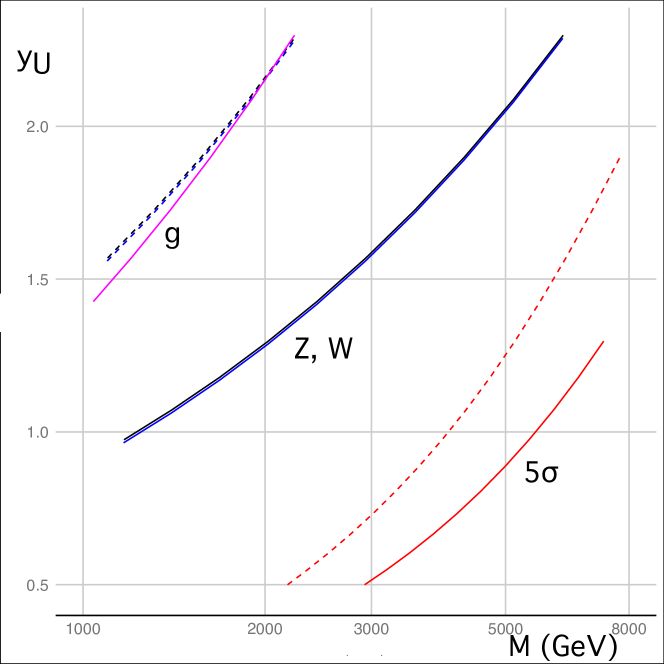
Figure 5: Mass reach for the deviation in the Higgs boson couplings due to integrating out a vectorlike quark doublet. The blue, black, and magenta curves indicate the 3 $\sigma$ contours for the deviation in the $HWW$, $HZZ$, and $Hgg$ couplings in a SMEFT fit to projected ILC data up to 500 GeV. The curves are plotted in the $(M,y_{U})$ plane for $y_{D}=0$ (dashed lines) and $y_{D}=y_{U}$ (solid lines). The red curves show the 5 $\sigma$ contour for the full SMEFT fit.

In Fig. 5, I plot the contours in the ($M,y_{U}$) plane along which individual Higgs boson couplings have a 3 $\sigma$ deviation from the Standard Model expectation, assuming measurements with the uncertainties expected for the 500 GeV ILC. The combination of these effects and others gives the contour for a 5 $\sigma$ deviation from the Standard Model which is also shown in the figure.

7 The $t$ squark-Higgsino system

Finally, as an example of a much more model-specific diagram that can lead to a significant effect, I discuss the stop-Higgsino loop correction to the $b$ quark Yukawa coupling. This is enhanced by the top quark Yukawa coupling, the (possibly heavy) higgsino mass, and the top quark $A$ term in the numerator. The correction is generated from the top quark Yukawa coupling but corrects the much smaller bottom quark Yukawa coupling. The effect occurs on top of other supersymmetry signals, such as those from the THDM structure, and it depends on its own specific parameter set. Thus, it is very difficult to understand the importance of this effect from general parameter scans of the MSSM model space. Here I give an estimate of its potential size, though it should be emphasized that treating this term in isolation is an oversimplification.

Begin from the diagram

(24)

which gives a loop correction to the $b$ quark mass or the $b$ quark Yukawa coupling. In principle, this diagram and the corresponding diagram with a $b$ squark could generate a large part of the $b$ quark mass. Thus, this example illustrates the possibility of large corrections to the Higgs couplings in models withmass generation by radiative feed-down. To give a nonzero effect, the diagram requires a helicity flip in the numerator of the Higgsino propagator, and a flip from $\tilde{t}_{R}$ to $\tilde{t}_{L}$ induced by the top squark $A$ term. When we expand this diagram in powers of a background field $H$, it also generates the dimension-6 operator ${\cal O}_{b}$ that corrects the $b$ quark Yukawa. Note that, for the similar diagram with a $b$ squark, the dimension-6 contribution is proportional to $m_{b}^{3}$ and thus is smaller by $(m_{b}/m_{t})^{2}$.

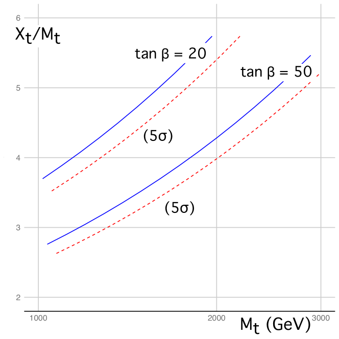
Figure 6: Mass reach for the deviation in the Higgs boson coupling to $b$ due to the diagram (24). The blue curves indicate the 3 $\sigma$ contours for the deviation in the $Hbb$ coupling in a SMEFT fit to projected ILC data up to 500 GeV. The curves are plotted in the $(M,X_{t}/M)$ plane for $\tan\beta=20,50$. The red curves show the 5 $\sigma$ contour for the full SMEFT fit.

In evaluating the diagram in (24), I make some simplifications. Since we are interested in heavy masses in the loop, I ignore terms in the $\tilde{t}$ and $\tilde{h}$ (mass²) matrices proportional to $m_{Z}^{2}$ and $m_{W}^{2}$. This, in particular, sets the charged Higgsino mass to $\mu$, which I take to be large. I also set the soft supersymmetry breaking masses of the $\tilde{t}_{R}$ and $\tilde{t}_{L}$ to be equal, with the value $M$. Then the top squark mass matrix is

$${\cal M}^{2}=\pmatrix{M^{2}&m_{t}X_{t}\cr m_{t}X_{t}&M^{2}\cr}\ ,$$ (25)

where $X_{t}=A_{t}-\mu\cot\beta$. I run $y_{t}(Q)$ to the scale $Q=M$; the running of $y_{b}$ from $m_{h}$ to $M$ cancels that of the generated dimension-6 operator running from $M$ to $m_{h}$. With these simplifications, the diagram leads to the effective operator

$$\Delta{\cal L}=-\Delta m_{b}\ \overline{b}_{L}\cdot H\,b_{R}$$ (26)

where

$$\Delta m_{b}=i{y_{b}y_{t}\over\sin\beta\cos\beta}\int{d^{4}p\over(2\pi)^{4}}{\mu\ m_{t}X_{t}\over(p^{2}-\mu^{2})((p^{2}-M^{2})^{2}-(m_{t}X_{t})^{2})}$$ (27)

and $X_{t}=A_{t}-\mu\cot\beta$. This operator is a function of the constant background Higgs field $H$. Expanding in $H$ reveals the correction to be a sum over operators of dimension 4, 6, etc. Carrying out this expansion, we find

$$\Delta{\cal L}=-\Delta y_{b}\overline{b}_{L}\cdot Hb_{R}-{c_{b}\over v^{2}}\,y_{b}|H|^{2}\overline{b}_{L}\cdot Hb_{R}-\cdots\ ,$$ (28)

with

$$\Delta y_{b} = {y_{b}y^{2}_{t}\mu\over\sin\beta\cos\beta}X_{t}\cdot(-i)\int{d^{4}p\over(2\pi)^{4}}{1\over(p^{2}-\mu^{2})(p^{2}-M^{2})^{2}}$$

$$c_{b}/v^{2}= = {y_{b}y_{t}^{2}\mu X_{t}^{3}\over\sin\beta\cos\beta}\cdot(-i)\int{d^{4}p\over(2\pi)^{4}}{1\over(p^{2}-\mu^{2})(p^{2}-M^{2})^{4}}$$ (29)

In particular,

$$c_{b} = -v^{2}\cdot{3\over 10}{y_{t}^{2}\mu X_{t}^{3}\over(4\pi)^{2}\sin\beta\cos\beta}$$ (30)

$$\hskip 36.135pt\cdot\biggl{[}{\mu^{6}-6M^{2}\mu^{4}+3M^{4}\mu^{2}+2M^{6}+6M^{4}\mu^{2}\log(\mu^{2}/M^{2})\over 2M^{4}(\mu^{2}-M^{2})^{4}}\biggr{]}$$

This expression predicts the largest effects when $\mu^{2}>M^{2}$, with both being much greater than $v^{2}$.

In Fig. 6, I plot the contours in the ($M,X_{t}$) plane along which individual Higgs boson couplings have a 3 $\sigma$ deviation from the Standard Model expectation, assuming measurements with the uncertainties expected for the 500 GeV ILC. Other Higgs factory proposals give very similar expectations. The contours are given for $M/\mu=0.5$ and $\tan\beta=20$, 50. The needed values of $X_{t}$ are large but not excessively so. According to [25], the instability to a color and charge breaking minimum is unimportant for such large values of the superpartner masses. The deviations due to this effect would typically add to deviations induced by other supersymmetry effects. For this reason, I draw the 5 $\sigma$ contours with dashed lines.

8 Conclusions

In this paper, I have shown that models of new physics can have signficant effects on the Higgs boson couplings even when the masses of the new particles that induce these effects are well beyond the direct search reach of the HL-LHC. This does not happen in all models, but it opens new classes of models and new regions of parameter space to exploration.

It is noteworthy that each model leads to its own pattern of deviations in the Higgs boson couplings, as was stressed in [1]. This implies that a discovery of deviations will also give information about the nature of the new physics that causes it.

In the best case, the regions of parameter space made accessible by precision Higgs measurements are beyond the scope of LHC searches today but within the scope of searches at the HL-LHC. Then discoveries at the HL-LHC and the Higgs factory can be truly complementary, reinforcing one another and offering different viewpoints on the nature of the new physics.

ACKNOWLEDGEMENTS

The results presented in this paper are part of a more general analysis in progress in collaboration with Ian Banta and Nathaniel Craig. I thank Ian and Nathaniel for suggesting this approach to the understanding of precision Higgs boson coupling mass reach, and for discussion of the results presented here. This analysis also benefited from insights and criticism from Christophe Grojean, Mihoko Nojiri, and Maxim Perelstein and from Sally Dawson, Patrick Meade, Laura Reina, and Caterina Vernieri. My work is supported by the US Department of Energy under contract DE–AC02–76SF00515.

References

- [1] T. Barklow, K. Fujii, S. Jung, R. Karl, J. List, T. Ogawa, M. E. Peskin and J. Tian, “Improved Formalism for Precision Higgs Coupling Fits,” Phys. Rev. D 97, 053003 (2018) [arXiv:1708.08912 [hep-ph]].
- [2] A. Aryshev et al. [ILC International Development Team], “The International Linear Collider: Report to Snowmass 2021,” [arXiv:2203.07622 [physics.acc-ph]].
- [3] M. Cahill-Rowley, J. Hewett, A. Ismail and T. Rizzo, “Higgs boson coupling measurements and direct searches as complementary probes of the phenomenological MSSM,” Phys. Rev. D 90, 095017 (2014) [arXiv:1407.7021 [hep-ph]].
- [4] A. Djouadi, J. Kalinowski and M. Spira, “HDECAY: A Program for Higgs boson decays in the standard model and its supersymmetric extension,” Comput. Phys. Commun. 108. 56 (1998). [arXiv:hep-ph/9704448 [hep-ph]], http://tiger.web.psi.ch/hdecay/.
- [5] X. Cid Vidal, M. D’Onofrio, P. J. Fox, R. Torre, K. A. Ulmer, A. Aboubrahim, A. Albert, J. Alimena, B. C. Allanach and C. Alpigiani, et al. “Report from Working Group 3: Beyond the Standard Model physics at the HL-LHC and HE-LHC,” CERN Yellow Rep. Monogr. 7, 585 (2019) [arXiv:1812.07831 [hep-ph]].
- [6] K. Fujii et al. [LCC Physics Working Group], [arXiv:1908.11299 [hep-ex]].
- [7] T. Barklow, K. Fujii, S. Jung, M. E. Peskin and J. Tian, “Model-Independent Determination of the Triple Higgs Coupling at e+e- Colliders,” Phys. Rev. D 97, 053004 (2018) [arXiv:1708.09079 [hep-ph]].
- [8] G. F. Giudice, C. Grojean, A. Pomarol and R. Rattazzi, “The Strongly-Interacting Light Higgs,” JHEP 06, 045 (2007) [arXiv:hep-ph/0703164 [hep-ph]].
- [9] R. K. Ellis, B. Heinemann, J. de Blas, M. Cepeda, C. Grojean, F. Maltoni, A. Nisati, E. Petit, R. Rattazzi and W. Verkerke, et al. “Physics Briefing Book: Input for the European Strategy for Particle Physics Update 2020,” [arXiv:1910.11775 [hep-ex]].
- [10] J. Bernon, J. F. Gunion, H. E. Haber, Y. Jiang and S. Kraml, “Scrutinizing the alignment limit in two-Higgs-doublet models: mh=125 GeV,” Phys. Rev. D 92, 075004 (2015) [arXiv:1507.00933 [hep-ph]].
- [11] H. E. Haber, “Nonminimal Higgs sectors: The Decoupling limit and its phenomenological implications,” [arXiv:hep-ph/9501320 [hep-ph]].
- [12] D. Egana-Ugrinovic and S. Thomas, “Effective Theory of Higgs Sector Vacuum States,” [arXiv:1512.00144 [hep-ph]].
- [13] H. Bélusca-Maïto, A. Falkowski, D. Fontes, J. C. Romão and J. P. Silva, “Higgs EFT for 2HDM and beyond,” Eur. Phys. J. C 77, no.3, 176 (2017) [arXiv:1611.01112 [hep-ph]].
- [14] CMS Collaboration, “Search for a new scalar resonance decaying to a pair of Z bosons at the High-Luminosity LHC,” CMS-PAS-FTR-18-040 (2019).
- [15] I. Banta, T. Cohen, N. Craig, X. Lu and D. Sutherland, “Non-decoupling new particles,” JHEP 02, 029 (2022) [arXiv:2110.02967 [hep-ph]].
- [16] B. Henning, X. Lu and H. Murayama, “How to use the Standard Model effective field theory,” JHEP 01, 023 (2016) [arXiv:1412.1837 [hep-ph]].
- [17] J. de Blas et al. [CLIC], “The CLIC Potential for New Physics,” [arXiv:1812.02093 [hep-ph]].
- [18] P. Huang, A. J. Long and L. T. Wang, “Probing the Electroweak Phase Transition with Higgs Factories and Gravitational Waves,” Phys. Rev. D 94, no.7, 075008 (2016) [arXiv:1608.06619 [hep-ph]].
- [19] S. Di Vita, C. Grojean, G. Panico, M. Riembau and T. Vantalon, “A global view on the Higgs self-coupling,” JHEP 09, 069 (2017) [arXiv:1704.01953 [hep-ph]].
- [20] G. Durieux, M. McCullough and E. Salvioni, “Charting the Higgs self-coupling boundaries,” [arXiv:2209.00666 [hep-ph]].
- [21] A. Angelescu and P. Huang, “Integrating Out New Fermions at One Loop,” JHEP 01, 049 (2021) [arXiv:2006.16532 [hep-ph]].
- [22] T. Han, H. E. Logan, B. McElrath and L. T. Wang, “Loop induced decays of the little Higgs: H — gg, gamma gamma,” Phys. Lett. B 563, 191 (2003) [erratum: Phys. Lett. B 603, 257 (2004)] [arXiv:hep-ph/0302188 [hep-ph]].
- [23] J. Hubisz, P. Meade, A. Noble and M. Perelstein, “Electroweak precision constraints on the littlest Higgs model with T parity,” JHEP 01, 135 (2006) [arXiv:hep-ph/0506042 [hep-ph]].
- [24] C. R. Chen, K. Tobe and C. P. Yuan, “Higgs boson production and decay in little Higgs models with T-parity,” Phys. Lett. B 640, 263 (2006) [arXiv:hep-ph/0602211 [hep-ph]].
- [25] A. Kusenko, P. Langacker and G. Segre, “Phase transitions and vacuum tunneling into charge and color breaking minima in the MSSM,” Phys. Rev. D 54, 5824 (1996) [arXiv:hep-ph/9602414 [hep-ph]].