Quantifying Aleatoric and Epistemic Uncertainty in Machine Learning:
Are Conditional Entropy and Mutual Information Appropriate Measures?

Abstract

The quantification of aleatoric and epistemic uncertainty in terms of conditional entropy and mutual information, respectively, has recently become quite common in machine learning. While the properties of these measures, which are rooted in information theory, seem appealing at first glance, we identify various incoherencies that call their appropriateness into question. In addition to the measures themselves, we critically discuss the idea of an additive decomposition of total uncertainty into its aleatoric and epistemic constituents. Experiments across different computer vision tasks support our theoretical findings and raise concerns about current practice in uncertainty quantification.

1 Introduction

Estimating, analyzing, and handling uncertainty has always been an integral part of classical statistics. More recently, the broader machine learning community has come to acknowledge its vital role in producing reliable estimates, which is, e.g., considered paramount in safety-critical applications [Senge et al., 2014, Kendall and Gal, 2017, Psaros et al., 2022]. In the context of supervised learning, the focus is typically on predictive uncertainty, i.e., the learner’s uncertainty about the outcome $y\in\mathcal{Y}$ given a query instance $\boldsymbol{x}$ from an input space $\mathcal{X}$. It is often expedient to decompose the total amount of uncertainty (TU) into its aleatoric (AU) and epistemic (EU) parts [Hüllermeier and Waegeman, 2021]. The aleatoric component of TU arises from the stochastic nature of the mapping from $\mathcal{X}$ to $\mathcal{Y}$, which implies that the “ground truth” is a (generally non-Dirac) conditional probability distribution $p(\cdot\,|\,\boldsymbol{x})$ over $\mathcal{Y}$. Potential sources of AU include measurement errors, randomness in physical quantities, and the simple fact that $\boldsymbol{x}$ may not suffice to explain $y$ [Malinin, 2019]. Thus, it is not possible to predict the outcome with certainty even assuming perfect knowledge of the data-generating process. In practice, the learner only finds an empirical estimate $\hat{p}(\cdot\,|\,\boldsymbol{x})$ from a pre-defined hypothesis space $\mathcal{H}$. Roughly speaking, EU then refers to a lack of knowledge about the discrepancy between $p$ and $\hat{p}$ that can – in contrast to AU – be alleviated by gathering more training samples [Senge et al., 2014]. Not least due to this potential reduction, the quantification of EU is helpful in many applications of AI, e.g., in order to invoke human intervention in multi-stage decision processes [Gal et al., 2017, Budd et al., 2021, Kirsch et al., 2022].

A specific set of measures for TU, AU, and EU has found broad consensus in the uncertainty quantification literature. Promoted by Houlsby et al. [2011] and Depeweg [2019], among others, the core idea revolves around Shannon entropy [Shannon, 1948] as a measure for TU, which can be shown to (additively) decompose into conditional entropy, interpreted as a measure of AU, and mutual information, resulting as a measure of EU [Kendall and Gal, 2017, Smith and Gal, 2018, Charpentier et al., 2022]. Various applications have recently used these measures (e.g., Michelmore et al. [2018], Shelmanov et al. [2021], Winkler et al. [2022]).

While the underlying ideas are well-established and mathematically well-founded, they originate from information theory and are not necessarily suited to uncertainty quantification in statistical learning. In fact, we find that the proposed entropy-related measures exhibit questionable behavior in a number of settings. We thus argue for a critical re-assessment of the established practice. Our contributions are as follows: We (i) point out numerous incoherencies of uncertainty measures based on decomposing Shannon entropy, (ii) shed light on why an additive disaggregation of TU might not be meaningful, and (iii) provide evidence for the relevance of these observations in practical applications.

2 Background

2.1 Uncertainty Representations

In the following, we assume categorical target variables from a finite label space $\mathcal{Y}=\{y_{1},\ldots,y_{K}\},K\in\mathbb{N}$. The set $\mathbb{P}(\mathcal{Y})$ of (first-order) probability distributions over $\mathcal{Y}$ can be identified with the ($K$-1)-simplex $\Delta_{K}\mathrel{\vbox{\hbox{\footnotesize.}\hbox{\footnotesize.}}}=\left\{\boldsymbol{\theta}=(\theta_{1},\ldots,\theta_{K})\in[0,1]^{K}\leavevmode\nobreak\ \,|\,\leavevmode\nobreak\ \|\boldsymbol{\theta}\|_{1}=1\right\}$. For each $\boldsymbol{\theta}\in\Delta_{K}$, we can compute an associated degree of AU [Hüllermeier and Waegeman, 2021]. To capture EU, the learner must be able to express uncertainty about $\boldsymbol{\theta}$, which can be accomplished by a (second-order) probability distribution over (first-order) distributions $\boldsymbol{\theta}$.

The canonical approach to such a bi-level representation is Bayesian inference, where uncertainty about the (Bayes) predictor is translated into uncertainty about a prediction expressed in terms of the posterior predictive distribution [Gelman et al., 2021]. Another idea is to estimate EU directly along with the prediction of the outcome. For instance, it is possible to learn the parameters of a Dirichlet distribution with a concentration parameter expressing EU [Malinin and Gales, 2018, Charpentier et al., 2020, Huseljic et al., 2020, Kopetzki et al., 2021]. Either way, we arrive at a second-order or second-order predictor $F:\mathcal{X}\longrightarrow\Delta_{K}^{(2)},$ where $\Delta_{K}^{(2)}=\mathbb{P}(\mathbb{P}(\mathcal{Y}))$ denotes the set of second-order distributions over $\mathcal{Y}$. For the sake of simplicity, we subsequently omit the conditioning on the query instance $\boldsymbol{x}$.

Each probability vector $\boldsymbol{\theta}\in\Delta_{K}$ implies a categorical distribution on $\mathcal{Y}$, such that $\theta_{k}=p(y_{k}\,|\,\boldsymbol{\theta})$ is the probability of outcome $y_{k}$, and one of these distributions, $\boldsymbol{\theta}^{\ast}$, corresponds to the (unknown) ground truth. If $F(\boldsymbol{x})=Q\in\Delta_{K}^{(2)}$ is the prediction for a query $\boldsymbol{x}$, then $Q$ assigns a probability $Q(\boldsymbol{\theta})$ to each distribution $\boldsymbol{\theta}\in\Delta_{K}$. $Q$ represents the epistemic state of the learner about $\boldsymbol{x}$, and a stronger concentration of $Q$ indicates more certainty about the true distribution $\boldsymbol{\theta}^{\ast}$. Note that we immediately regard the output distribution and omit from our notation any relation to objects that play a role in estimating $\boldsymbol{\theta}$ (e.g., the Bayes posterior is often expressed as a distribution over model parameters given data).

As an example, consider the case of binary classification ($K=2$), where $\mathcal{Y}=\{y_{0},y_{1}\}$ consists of only two classes, negative and positive (illustrated in Fig. 1). The conditional distribution $p(\cdot\,|\,\boldsymbol{x})$ is now determined by the probability vector $\boldsymbol{\theta}=(\theta_{0},\theta_{1})=(p(y_{0}\,|\,\boldsymbol{x}),\leavevmode\nobreak\ p(y_{1}\,|\,\boldsymbol{x}))$. As the individual class probabilities sum up to one, prediction in $\boldsymbol{x}$ effectively comes down to inference about the ground-truth probability $\theta_{1}^{\ast}=p(y_{1}\,|\,\boldsymbol{x})$ of the positive class, and hence about the success parameter $\theta$ of a Bernoulli distribution $\mathcal{B}(\theta)$. The corresponding second-order distribution $Q$ could be, for example, a Beta distribution (or, more generally, a Dirichlet distribution for $K\geq 2$).

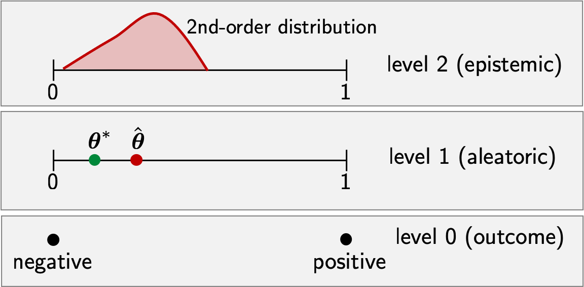
Figure 1: Bi-level uncertainty representation in binary classification. We pose a second-order distribution $Q$ over Bernoulli distributions corresponding to the probability $\theta$ of the positive class. In Bayesian inference, $Q$ is given by the posterior distribution (epistemic level), and a point prediction $\hat{\theta}$ (aleatoric level) is obtained by model averaging. On level zero, only binary class labels are observed.

2.2 Entropy-Based Information Measures

Given a representation of an uncertain prediction in terms of a second-order distribution $Q$, one is often interested in quantifying the learner’s uncertainty in terms of a single number, and decomposing the TU into its aleatoric and epistemic contributions. One approach that is now commonly adopted [Houlsby et al., 2011, Gal, 2016, Depeweg et al., 2018, Smith and Gal, 2018, Mobiny et al., 2021] is based on information-theoretic quantities derived from Shannon entropy. Let $Y$ signify the random outcome variable with marginal probability

$$p(y)=\textstyle\int_{\Delta_{K}}p(y\,|\,\boldsymbol{\theta})\,\operatorname{d}Q(\boldsymbol{\theta}).$$ (1)

The (discrete) Shannon entropy of $Y$ can be defined as

$$H(Y)=-\textstyle\sum_{y\in\mathcal{Y}}p(y)\cdot\log p(y)\,,$$ (2)

where the logarithm is typically set to base 2. For continuous label spaces, we obtain the differential entropy analogously by replacing the sum in Eq. (2) with an integral over $\mathcal{Y}$ [Cover and Thomas, 2006].

Shannon entropy can be interpreted as the degree of uniformity in the distribution of a random variable, or the amount of information to be gained from observing its realization (further analogies exist in physics and source coding). It enjoys a number of desirable properties: it is non-negative, maximal for the uniform distribution, and invariant to permutations of classes in $\mathcal{Y}$ [Cover and Thomas, 2006].

Exploiting the fact that $Y$ is the expectation of the conditional outcome (given $\boldsymbol{\theta}$) with respect to the second-order distribution $Q$, the Shannon entropy, as a measure of TU, can be computed as

$$H(Y) =H\big{(}\mathbb{E}_{Q}\left[Y\,|\,\boldsymbol{\theta}\right]\big{)}.$$ (3)

A trivial result from information theory states that Shannon entropy additively decomposes into conditional entropy and mutual information (e.g., Ash [1965]):

$$H(Y)=H(Y\,|\,\Theta)+I(Y,\Theta).$$ (4)

Here, $\Theta$ denotes the random variable of first-order distributions $\boldsymbol{\theta}\sim Q$. Conditional entropy $H(Y\,|\,\Theta)$ expresses the uncertainty about $Y$ that would remain if the realization of $\Theta$ were known, and is therefore taken to quantify AU. The motivation for expressing AU this way is as follows: By fixing a first-order distribution $\boldsymbol{\theta}\in\Delta_{K}$, all EU is essentially removed and only AU remains, such that $H(Y\,|\,\boldsymbol{\theta})=-\sum_{k=1}^{K}\theta_{k}\,\log\theta_{k}$ is indeed a natural measure of AU. However, as $\boldsymbol{\theta}$ is not precisely known, we take the expectation with respect to the second-order distribution:

$$H(Y\,|\,\Theta) =\mathbb{E}_{Q}\left[H\left(Y\,|\,\boldsymbol{\theta}\right)\right]$$ (5)

$$=\textstyle\int\limits_{\Delta_{K}}\underbrace{\textstyle\sum_{y\in\mathcal{Y}}-p(y\,|\,\boldsymbol{\theta})\log p(y\,|\,\boldsymbol{\theta})}_{H(Y\,|\,\boldsymbol{\theta})}\,\operatorname{d}Q(\boldsymbol{\theta}).$$

Mutual information $I(Y,\Theta)$, proposed to embody EU, is a symmetric measure for the expected information gained about one variable through observing the other and vanishes if both variables are independent. Intuitively, it quantifies the potential reduction in uncertainty about $Y$ through observing $\Theta$ [Ash, 1965]:

$$I(Y,\Theta) =H(Y)-H(Y\,|\,\Theta)$$

$$=\mathbb{E}_{Q}\left[D_{\text{KL}}\left(p(Y|\Theta)\leavevmode\nobreak\ \|\leavevmode\nobreak\ p(Y)\right)\right].$$ (6)

2.3 Finite-Ensemble Approximation

In practice, it will hardly be possible to compute exact expectations with respect to $Q$ due to the intractability of the corresponding integrals, so we must permit some kind of approximation. The standard approach to this problem is Monte Carlo integration with a finite number $M\in\mathbb{N}$ of samples $\boldsymbol{\theta}\sim Q$, whose induced mean, by the law of large numbers, almost surely converges to the true integral [Andrieu et al., 2003]. In machine learning, this way of combining the predictions of multiple models is common practice and known as ensemble learning (e.g., Breiman [2001], Lakshminarayanan et al. [2017]). For TU, the entropy over the approximate first-order distribution becomes

$$H(Y)=H\left(\tfrac{1}{M}\textstyle\sum_{m=1}^{M}p\left(y\,|\,\boldsymbol{\theta}^{(m)}\right)\right),$$ (7)

where $\boldsymbol{\theta}^{(m)}$, $m\in\{1,\ldots,M\}$, is the prediction of the $m$-th ensemble member. Analogously, we obtain the ensemble conditional entropy as a measure of AU:

$$H(Y\,|\,\Theta)=\tfrac{1}{M}\textstyle\sum_{m=1}^{M}H\left(p\left(y\,|\,\boldsymbol{\theta}^{(m)}\right)\right).$$ (8)

The discrete EU is the Jensen-Shannon divergence

$$\tfrac{1}{M}\textstyle\sum_{m=1}^{M}D_{\text{KL}}\left(p\left(y\,|\,\boldsymbol{\theta}^{(m)}\right)\,\Big{\|}\,\tfrac{1}{M}\textstyle\sum_{j=1}^{M}p\left(y\,|\,\boldsymbol{\theta}^{(j)}\right)\right).$$ (9)

Finite-ensemble EU still results as the difference between Eq. (7) and Eq. (8) under the conditions of Section 2.2. Obviously, ensemble learning provides a rather coarse approximation to the expectation $\mathbb{E}_{Q}(\cdot)$, especially if the size $M$ of the ensemble is small. Consider, for example, deep ensembles [Lakshminarayanan et al., 2017], which have become a de facto gold standard in probabilistic machine learning [Ovadia et al., 2019, Ashukha et al., 2020, Psaros et al., 2022]. The cost of training each of their neural network members is typically so high that $M$ remains in the realm of five to ten (e.g., Abe et al. [2022], Turkoglu et al. [2022]). We must then expect certain (low-density) regions in the space of first-order distributions to be systematically undersampled, affecting the estimate of EU in particular.

3 Related Work

The decomposition in Eq. (4) is widely applied and often used in conjunction with Bayesian learning, e.g., to obtain more robust predictions by explicitly modeling both components of TU [Kendall and Gal, 2017], to design better optimization procedures by using the decomposition in stochastic differential equations [Winkler et al., 2022], or to improve the general understanding of neural networks [Woo, 2022]. In natural language processing, Wu et al. [2020] filter unreliable predictions in spoken language assessment caused by high EU, while Shelmanov et al. [2021] perform active learning with EU-based acquisition for label-efficient sequence tagging. Further fields of application include autonomous driving, where EU is found to be predictive of forthcoming accidents [Michelmore et al., 2018], and medical diagnostics, with a focus on identifying inherently ambiguous cases [Mobiny et al., 2021].

We find, however, that the entropy decomposition may lead to unintended results discussed in the subsequent section. While we do not dispute the mathematical correctness of Eq. (4)-(2.2), we argue that the individual quantities and their additive aggregation are not suitable for evaluating predictive uncertainty. Although previous work uncovered similar shortcomings of measures in related uncertainty frameworks (e.g., Pal et al. [1992] on evidential reasoning), the entropy-based measures – to the best of our knowledge – have drawn hardly any criticism in the machine learning community. In the following, we point out numerous inconsistencies that cast doubt on the usefulness of the individual measures and address the more general issue of additive decomposition.

4 Critical Assessment

Let TU, AU, and EU denote, respectively, measures $\Delta_{K}^{(2)}\longrightarrow\mathbb{R}$ of total, aleatoric, and epistemic uncertainty associated with a (second-order) uncertainty representation $Q\in\Delta_{K}^{(2)}$. In the literature, it is common to define the fundamental properties of uncertainty measures through an axiomatic approach (see also, for example, Bronevich and Klir [2008], Pal et al. [1993]. In the following, we define some properties these measures should naturally satisfy.

• TU, AU, and EU are non-negative.

• EU vanishes for Dirac measures $Q=\delta_{\boldsymbol{\theta}}$.

• EU and TU are maximal for $Q$ being the uniform distribution on $\Delta_{K}^{(2)}$.

• If $Q^{\prime}$ is a mean-preserving spread of $Q$, then $\text{EU}(Q^{\prime})\geq\text{EU}(Q)$ (weak version) or $\text{EU}(Q^{\prime})>\text{EU}(Q)$ (strict version); the same holds for TU.

• If $Q^{\prime}$ is a center-shift of $Q$, then $\text{AU}(Q^{\prime})\geq\text{AU}(Q)$ (weak version) or $\text{AU}(Q^{\prime})>\text{AU}(Q)$ (strict version); the same holds for TU.

• If $Q^{\prime}$ is a spread-preserving location shift of $Q$, then $\text{EU}(Q^{\prime})=\text{EU}(Q)$.

4.1 Total Uncertainty

Although Shannon entropy is widely established as a measure of uncertainty associated with a random variable, one may wonder about its appropriateness for quantifying total predictive uncertainty in the scenario outlined above. As an illustration, we pick up our previous example of binary classification (note that properties A0-A5 apply to $Q,Q^{\prime}\in\Delta_{K}^{(2)}$ but violations for $K=2$ suffice to conclude that they do not hold in general). Fig. 2 shows some exemplary second-order distributions $Q$ together with the values they induce for TU, AU, and EU about the prediction of $\theta$.

We first note that property A3 is violated by TU in terms of entropy, at least in its strict version, because (3) depends on $Q$ only through its expectation.

Proposition 1.

Total uncertainty defined in terms of Shannon entropy (3) violates the strict version of A3.

For example, in the special case $Q\in\Delta_{2}^{(2)}$, $H(Y)$ is maximal as soon as $Q$ is symmetric around $\theta=\tfrac{1}{2}$. Consequently, the uniform distribution on the unit interval, $Q=\mathcal{U}[0,1]$ (Fig. 2a), which is commonly considered a representation of complete ignorance (justified by the “principle of indifference” invoked by Laplace, or by referring to the principle of maximum entropy), has the same TU as a mixture of Dirac distributions $Q=\tfrac{1}{2}\delta_{0}+\tfrac{1}{2}\delta_{1}$ (Fig. 2f) dividing all probability mass between the outcomes $\theta=0$ and $\theta=1$. While one may argue that the uncertainty about the target variable $Y$ is indeed the same in both cases, it seems counter-intuitive to obtain identical results when in one scenario, the learner (supposedly) knows nothing, whereas, in the other, it has substantial knowledge about the ground-truth distribution $\theta^{\ast}$. Likewise, it appears strange that any distribution $Q$ not symmetric around $\tfrac{1}{2}$ will have a lower TU, including, for example, $\mathcal{U}[0.45,0.85]$ (Fig. 2e), when it arguably represents a lower degree of informedness than the Dirac mixture.

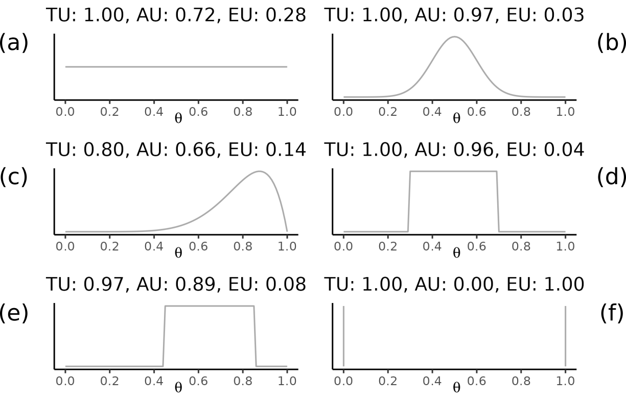
Figure 2: Different second-order distributions $Q$ over the parameter $\theta$ of a Bernoulli distribution with associated uncertainty. (a) $\mathcal{U}[0,1]$; (b) $\mathcal{N}(0.5,0.01)$; (c) $\operatorname{Beta}(8,2)$; (d) $\mathcal{U}[0.3,0.7]$; (e) $\mathcal{U}[0.45,0.85]$; (f) $\tfrac{1}{2}\delta_{0}+\tfrac{1}{2}\delta_{1}$.

The root cause of these peculiarities is the role of the distribution $Q$ in the computation of TU – effectively, $Q$ is marginalized over. In this sense, the reason for having maximal TU in the case of $\mathcal{U}[0,1]$ is not that it (supposedly) encodes the greatest lack of knowledge, but only its symmetry around $\theta=\tfrac{1}{2}$. Information about the second-order distribution is thus compressed to a single number in the form of its expectation. On the other hand, the concentration of $Q$ is hardly reflected in the TU, although it should be an important indicator of the learner’s state of knowledge.

4.2 Aleatoric Uncertainty

Noting that, in Eq. (5), $Q$ represents the learner’s subjective belief about a supposedly objective ground-truth $\boldsymbol{\theta}^{\ast}$ associated with query $\boldsymbol{x}$, $H(Y\,|\,\Theta)$ can be seen as the learner’s (current) best guess of the true AU. Although this might seem a sensible quantity, the relationship between this estimate and the true AU, $H(Y\,|\,\boldsymbol{\theta}^{\ast})$, is by no means clear. The problem is that AU estimates – even if the additive nature of the decomposition might suggest otherwise – cannot be separated from the learner’s epistemic state. In the finite-sample case, the learner must fall short of perfect knowledge, meaning that its belief $Q$ will not coincide with the Dirac distribution on $\boldsymbol{\theta}^{\ast}$ that represents the true second-order distribution. This, however, directly translates to the estimate of AU that is derived by taking the expectation over $Q$. Whenever there is EU, we must expect the AU estimation to be compromised, and the absence of a ground-truth precludes us from knowing how it is affected exactly.

In particular, conditional entropy is neither a true expectation nor a lower or upper bound on the true AU, and the resulting point estimate suggests a degree of informedness that is hardly justified. The limited ability of probability distributions to properly distinguish between different subjective beliefs adds to the problem. For example, if a uniform $Q$ is meant to represent complete ignorance, then all the learner can infer is that the true AU is between zero (for $\theta\in\{0,1\}$) and one (for $\theta=\tfrac{1}{2}$). This is clearly a different situation than having perfect knowledge about all first-order distributions being equally probable. Ultimately, however, both lead to the same average over the support of $Q$. Therefore, we must conclude that AU is computed with respect to a belief that the second-order distribution may fail to express, and that must be expected to be wrong.

4.3 Epistemic Uncertainty

The definition of mutual information (Eq. (2.2)) may appear intuitively plausible at first sight: If the observation of $Y$ reveals a sizeable amount of information about $\Theta$, then the learner’s uncertainty about $\Theta$ must be high (et vice versa). Likewise, a high divergence in the finite-ensemble version (Eq. (9)), i.e., in the predictions of different ensemble members, can be viewed as indicating a high EU.

That said, the measures do not necessarily behave as one may expect. Looking at Fig. 2, a first observation is that EU tends to be relatively low, which is especially noticeable in the case of the standard uniform distribution (upper left). As already mentioned, $\mathcal{U}[0,1]$ is usually meant to represent complete ignorance, suggesting that the learner is as uninformed as it could be, so we would expect a measure of EU to fulfill property A2 (i.e., be maximal) in this case.

Proposition 2.

EU in terms of mutual information $I(Y,\Theta)$ violates property A2.

This violation holds in general, and can be seen very easily for the case $K=2$ in Fig. 2. In Bayesian inference, for example, the uniform distribution is commonly adopted as a prior, representing knowledge before seeing any data. In such a state, one would assume all uncertainty to epistemic, and hence the measure of EU to be very high. On the contrary, however, AU (at 0.72) is well above EU (at 0.28). Actually, the maximal EU (1.00) is reached only for the case of Fig. 2f, in which $Q$ is a mixture of two Dirac measures, one placed at $\theta=0$ and the other at $\theta=1$. This distribution suggests a deterministic dependency, where the outcome is either certainly positive or certainly negative – a case in which the learner undoubtedly knows more than nothing, so again, the level of EU does not seem appropriate.

Also, note that EU is not invariant against a location shift of the distribution $Q$, even though it would be reasonable to expect that EU remains constant when the spread of $Q$ does not change.

Proposition 3.

There exist location shifts $Q^{\prime}\in\Delta_{K}^{(2)}$ of $Q\in\Delta_{K}^{(2)}$ such that property A5 is violated.

For example, the distributions in Fig. 2d and Fig. 2e (case $K=2$) are both uniform on an interval of length 0.4, suggesting the same level of informedness about the ground truth $\theta$. However, the respective degrees of EU (0.04 vs. 0.08) differ. Of course, one may argue that the uncertainty will depend not only on the shape but also on the location of the distribution. Then, however, $\mathcal{U}[0.3,0.7]$ should arguably exhibit higher uncertainty, as it puts more probability mass close to $\theta=\tfrac{1}{2}$ than $\mathcal{U}[0.45,0.85]$. This is indeed the case for TU and AU but exactly reversed for EU.

Lastly, we would expect EU to increase when $Q$’s mass is spread over a larger support (all else being equal), such that more hypotheses are deemed likely. Such spreading happens, for example, in moving from $\tfrac{1}{2}\delta_{0.45}+\tfrac{1}{2}\delta_{0.95}$ to $\mathcal{U}[0,1]$, while EU actually gets higher rather than lower.

Proposition 4.

EU in terms of mutual information $I(Y,\Theta)$ violates property A3.

Mathematically, the numbers are clearly correct and meaningful: In Fig. 2f, for example, the ground-truth distribution $\theta$ is uniquely determined as soon as the outcome $Y$ has been observed, so mutual information should be maximal. What must be concluded is rather that mutual information may not be the right measure of EU. Indeed, mutual information is arguably more a measure of divergence or conflict than of ignorance, as the common understanding of EU would suggest. This is quite obvious from Eq. (2.2) and even easier to see in the discrete version (Eq. (9)) for finite ensembles. Mutual information effectively quantifies the expected divergence of single hypotheses from the opinion given by integrating over all of them. Consequently, it is much higher for the Dirac mixture in Fig. 2f, with maximal divergence of both hypotheses from the average $\theta=\tfrac{1}{2}$, than for $\mathcal{U}[0,1]$, which also assigns probability mass to many alternatives that diverge only little from the expectation. Thus, mutual information behaves as expected but does not seem well-suited to measuring a quantity taken to represent ignorance.

4.4 Additive Decomposition

Let us conclude this section with a few remarks on another potential problem of uncertainty quantification, which is related, though not restricted, to the quantification discussed in this paper. According to Eq. (4), TU (entropy) decomposes additively into AU (conditional entropy) and EU (mutual information). When combining distinct sources of uncertainty, additive representations of this kind appear natural and can also be found for other measures of uncertainty, such as variance (see, e.g., Depeweg et al. [2018] for a discussion of entropy and variance decomposition). However, when considering Eq. (4) in a machine learning setting, where the (total) uncertainty is not fixed but decreases with increasing sample size, additivity might be less obvious because the aleatoric part does not correspond to the true AU, but only to an estimate thereof. Moreover, this estimate depends on the EU, such that the two measures are tightly interwoven and certainly not independent of each other. So, what is the justification for simply adding them up?

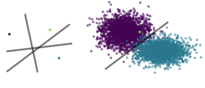
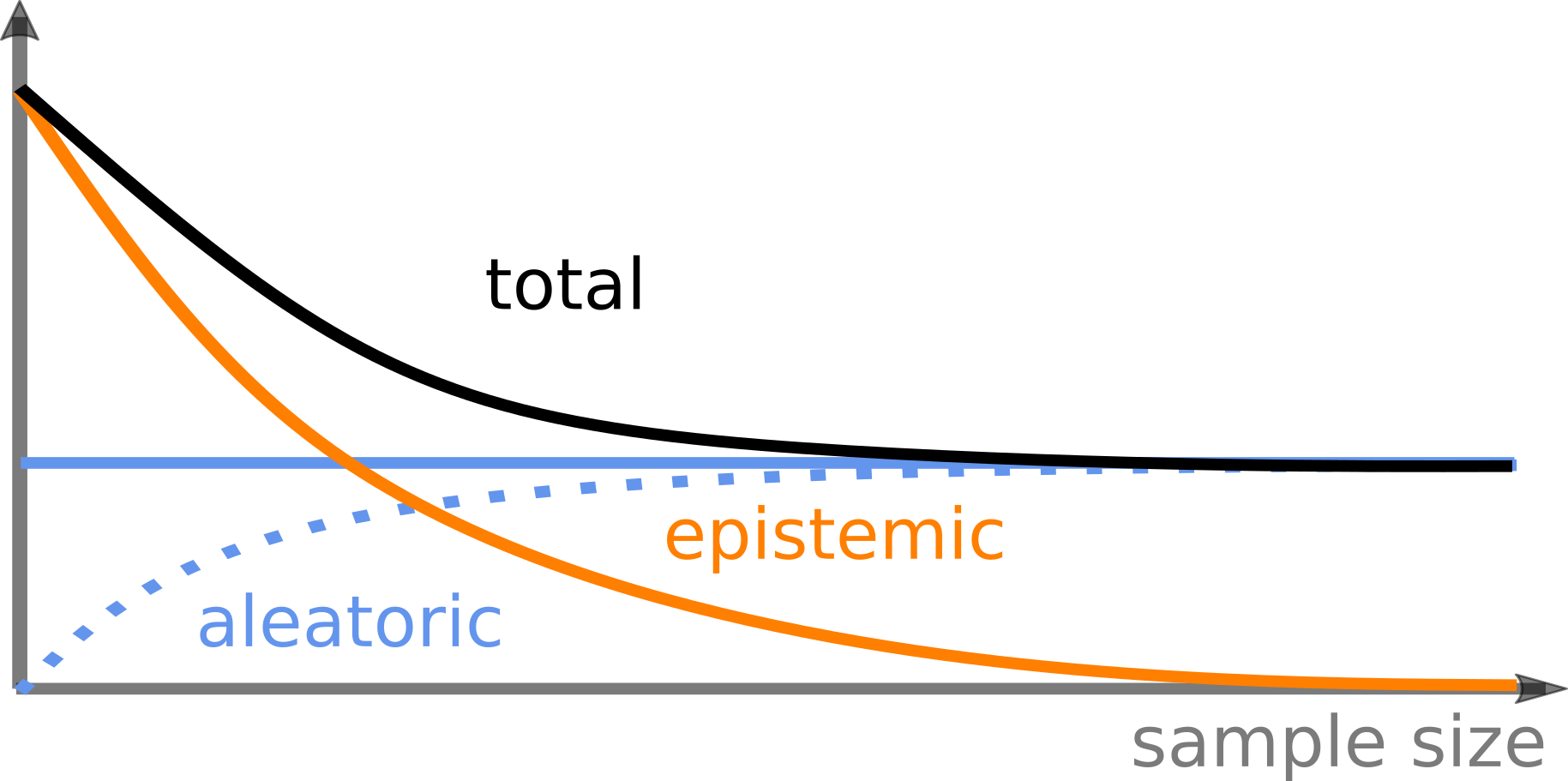
Figure 3: In the beginning, the learner is very uncertain about the true class probability for the (green) query point $\boldsymbol{x}$ (top-left), but this (epistemic) uncertainty disappears with increasing sample size (top-right). The bottom plot shows the expected qualitative behavior of uncertainty components. The dotted line marks the difference of TU and EU (which equals AU when stipulating additivity).

The dependence between the measures can be seen most clearly at the beginning of a learning process, during which the number of observed samples increases when the learner has seen very little or even no data. For example, take the case of binary classification, where the learner is still fully ignorant about the probability $\theta=p(y_{1}\,|\,\boldsymbol{x})$ of the positive class in a certain point $\boldsymbol{x}$: it might be a clear positive case ($\theta=1$), a clear negative case ($\theta=0$), but also everything in between. In this situation, an ideal measure of TU should arguably assume its maximum value. Likewise, an ideal measure of EU should be maximal because the learner is as uninformed about $\theta$ as it can be (note this is not the case for mutual information when starting with a uniform prior). Then, however, additivity implies that AU must be zero, at least if the measures share a common scale with the same maximum value (which holds for entropy and mutual information). In a sense, the aleatoric part is already comprised in the epistemic part, suggesting that the difference between TU and EU can, at best, be interpreted as a lower bound to the true AU. This is depicted graphically in Fig. 3: With a growing sample size, we expect EU to decrease and eventually vanish because the learner will gain full knowledge about the data-generating process, while both TU and TU minus EU should converge to the true AU (the former from above and the latter from below).

The above can be summarized as follows:

Proposition 5.

If EU and TU attain their respective maxima at the beginning of learning, and they are constructed to be on the same scale, then TU cannot decompose additively into EU and AU if AU is positive.

What these considerations suggest is that, in the finite-sample (machine learning) regime, additivity might inevitably be violated by “ideal” measures of TU, EU, and (ground-truth) AU (again, note that entropy and mutual information with a uniform prior are not ideal in this sense, which is what we criticized them for). Instead, additivity may only hold for the decomposition of TU into EU and a lower bound to AU, or might be relaxed to sub-additivity along the lines of Dubois et al. [1996]. Alternatively, additivity must be preserved by giving up other assumptions, e.g., that all measures share the same scale. Recently, for example, Hüllermeier et al. [2022] proposed a decomposition for the uncertainty of sets of probability distributions (credal sets), in which EU can become twice as high as AU.

5 Experiments

5.1 Experimental Setup

We conduct a number of experiments that provide practical evidence about the incoherent behavior of entropy-based uncertainty measures. For further details on training configurations, see supplementary material A. The experimental code is available in full via a public repository.

Datasets

We consider image classification tasks for two real-world datasets, CIFAR10 [Krizhevsky, 2009] and MNIST [LeCun et al., 1998], containing ten classes of color and gray-scale images, respectively. For a setting over which we can exert full control, we further synthesize black-and-white images of rectangles, where one class is characterized by vertical extension (i.e., height $>$ width) and the other vice versa, and simulate a bivariate classification problem with tabular features and four classes.

Probabilistic Learners

For the computer vision tasks, we employ deep ensembles of $M$ neural networks with varying random initialization [Lakshminarayanan et al., 2017], as well as a Laplace approximation [Daxberger et al., 2021] that fits a Gaussian approximate posterior to the location of the maximum-a-posteriori estimator and draws $M$ samples from this distribution. Furthermore, we train a random forest [Breiman, 2001] and an ensemble of single-hidden-layer feedforward neural networks (MLPs) for the tabular classification problem. Ensemble predictions are computed by averaging over the outputs of individual members. We set $M=10$. While this may seem small, note that this is in accordance with common practice (e.g., Beluch et al. [2018], Lee et al. [2021], Abe et al. [2022], Kristiadi et al. [2022], Turkoglu et al. [2022]) because larger ensembles are rarely affordable in the deep learning with architectures typically numbering in the millions. Our ablations suggest that the observed qualitative behavior is fairly robust with respect to ensemble size (see supplementary material B.2).

Evaluation

The figures in the following paragraphs visualize estimates for AU, EU, and TU (normalized to values in $[0,1]$) alongside predictive performance in terms of accuracy (ACC) and expected calibration error (ECE; Naeini et al. [2015]). The uncertainty estimates are depicted as lines (averaged over all test samples, left $y$-axis), while the bars represent performance (right $y$-axis). All results are aggregrated over three independent runs, with error bars on the uncertainty curves indicating one standard deviation.

5.2 Results and Discussion

5.2.1 Increasing Sample Size

We first study how the components of total Shannon entropy evolve with sample size, where we admit increasingly larger training datasets from 1% to 100% of available samples (randomly selected; the classes are balanced).

Expected Behavior

TU and EU start from their highest level and decrease gradually, while AU approaches its true constant value from below (due to the additivity assumption). The reported uncertainty is higher when accuracy is low.

Observed Behavior

We observe the expected downward slope of TU and EU as a general pattern, but the evidence is otherwise not quite consistent. Most strikingly, the AU estimates also assume high initial values and decrease for larger sample size in three out of four cases. For CIFAR10, this behavior is clearly visible (Fig. 5), underlining our concern that AU estimates are unreliable in the light of limited knowledge. In the case of MNIST and the deep ensemble, uncertainty is ultra-low from the beginning, but a close-up in the small overlaying plot of Fig. 4 (top) reveals the same trend. Reported EU for small sample sizes seems quite low overall, despite limited information and consequently poor performance. A notable exception is the Laplace approximation for MNIST (Fig. 4, bottom), which resembles most closely what we would have expected, though it appears more susceptible to random changes (see close-up).

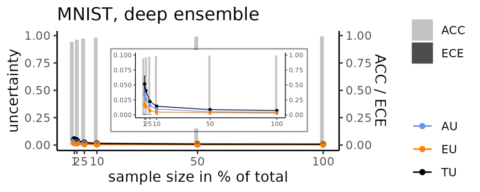
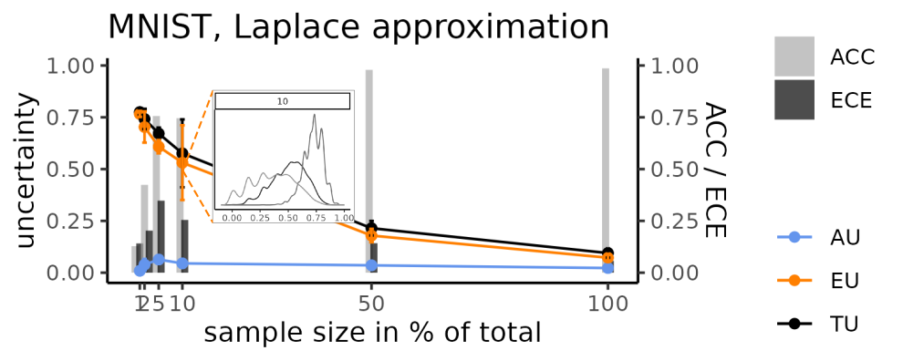
Figure 4: Entropy-based uncertainty for increasing sample size (MNIST). Overlaying plot (top): re-scaled left $y$-axis. Overlaying plot (bottom): empirical densities of observed instance-wise EU values (each curve represents one run of the experiment) with 10% sample size.

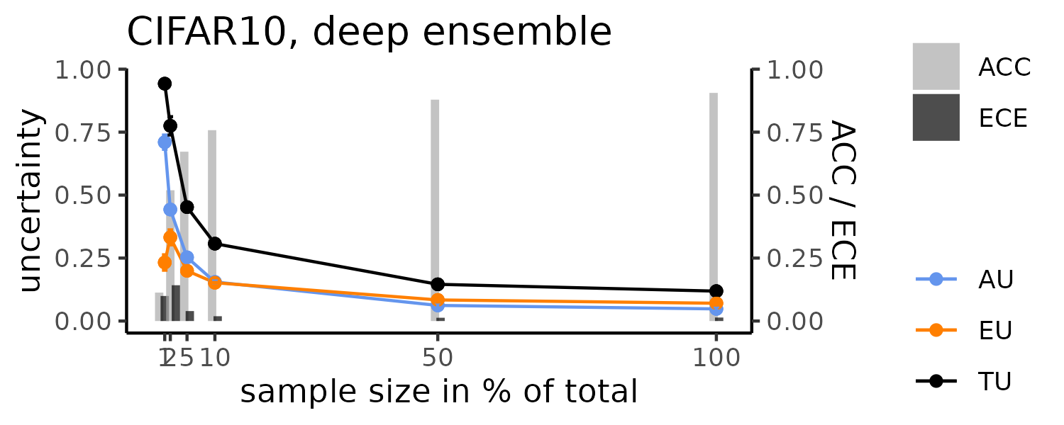
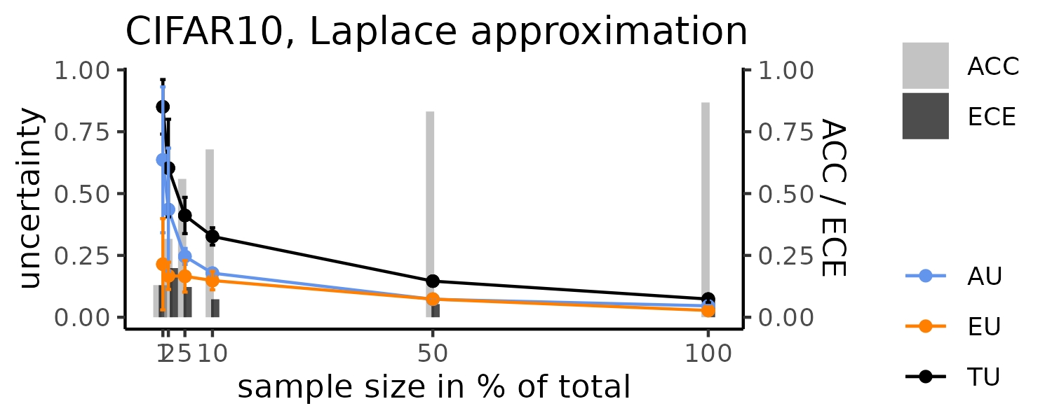
Figure 5: Entropy-based uncertainty for increasing sample size (CIFAR10).

5.2.2 Increasing Data Noise

Next, we modify the level of noise in the data, for which we use different proxies. First, we vary image resolution in the computer vision tasks by downscaling (original sizes: 28$\times$28 / 32$\times$ 32 for MNIST / CIFAR10); second, we shrink the relative class distance for the tabular data and thus enforce stronger overlap (Fig. 6); and lastly, we randomly change class labels for a varying share of observations in the same dataset (see supplementary material B.1).

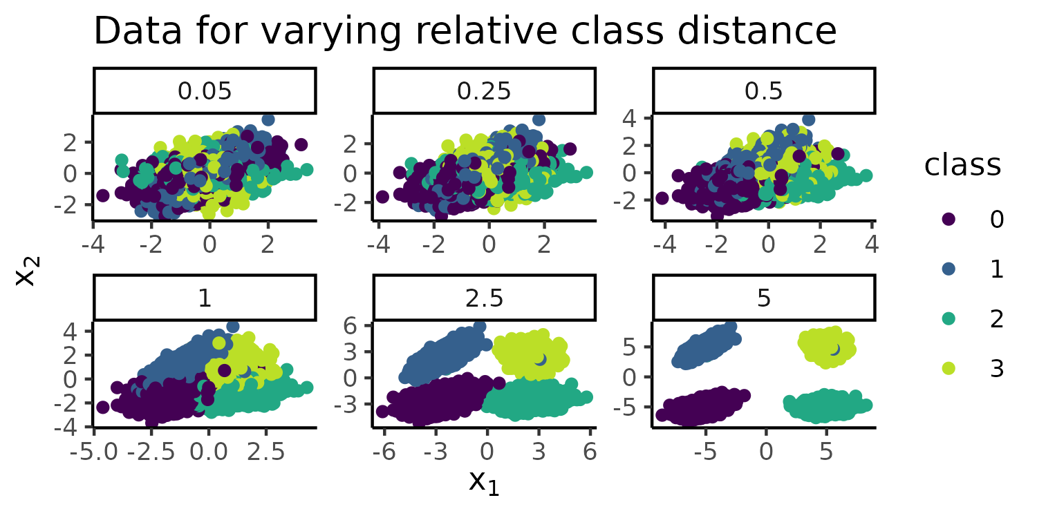
Figure 6: Tabular data with two features and four classes for increasing class overlap.

Expected Behavior

AU picks up with increasing noise level. Since learner capacity remains fixed, it is reasonable to assume that EU also rises to some extent when the decision boundaries become more complex with mounting degree of dataset contamination.

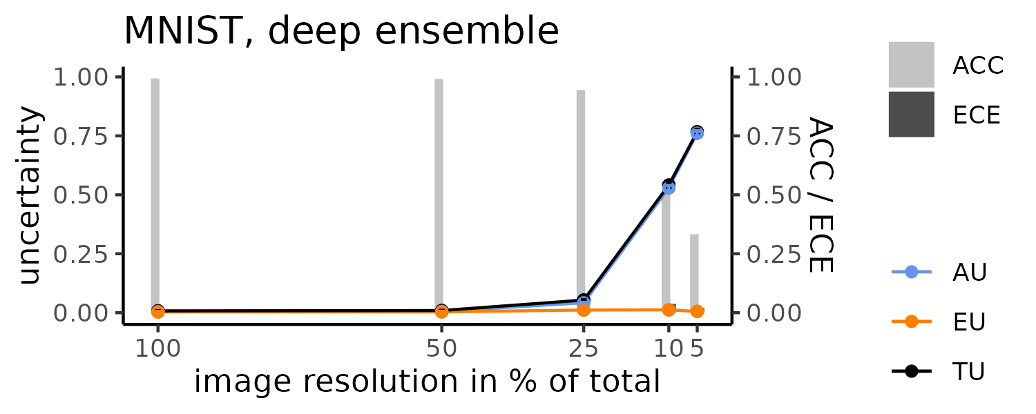
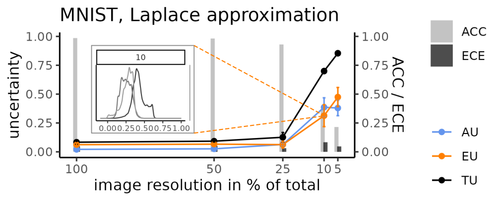
Figure 7: Entropy-based uncertainty for decreasing image resolution (MNIST). Overlaying plot: empirical densities of observed instance-wise EU values (each curve represents one run of the experiment) with 10% resolution.

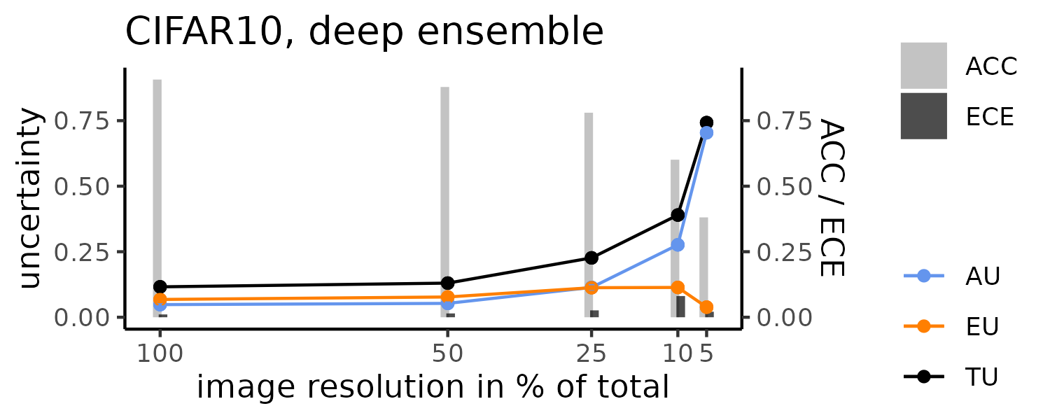
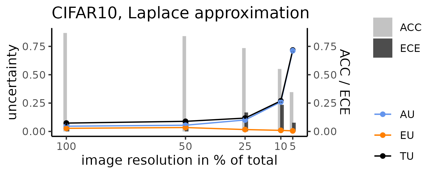
Figure 8: Entropy-based uncertainty for decreasing image resolution (CIFAR10).

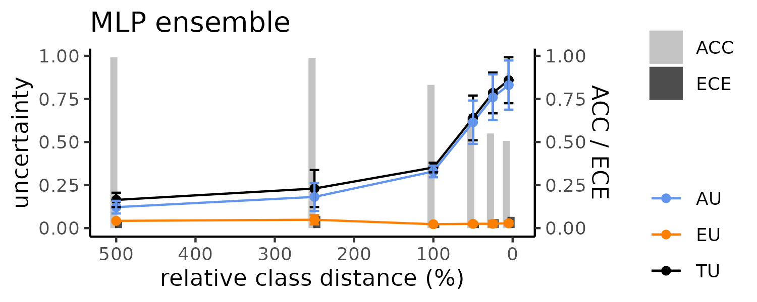
Figure 9: Entropy-based uncertainty for for increasing class overlap (tabular data).

Observed Behavior

More noise indeed prompts a rise in AU in all cases (Fig. 7-9). However, EU remains basically constant and very low, even when the data are so noisy that performance plummets. Note that, for instance, 10% resolution corresponds to a compression into 3$\times$3 pixels for both MNIST and CIFAR10, and how the decision boundaries become quite blurred in the tabular dataset when classes overlap more strongly (Fig. 6). Again, the Laplace approximation for MNIST is something of an exception: here, EU increases for the lowest resolution values, but leaves AU remarkably small and even falling from 10% to 5% resolution. We find thus that the uncertainty measures behave, if not entirely implausible, again somewhat inconsistently.

5.2.3 Test Distribution Shift

Following a slightly different idea than in the previous experiment, we now train the learner on a well-separated dataset of synthetic rectangles and seek predictions for instances which interpolate between the classes. This is achieved by decreasing the rectangles’ side-length ratio, effectively pushing them towards a square.

We further present the learner with samples that are from an entirely different class, namely random non-convex polygons with 3–5 vertices, and thus out-of-distribution (OOD) relative to the training data. Both settings create a form of distribution shift between training and test data that is associated with the presence of predictive uncertainty.

Expected Behavior

Class interpolation mainly affects AU through instances located close to the learned decision boundaries. In OOD detection, demanding predictions for samples from a previously unseen class should spike an increase in EU.

Observed Behavior

The deep ensemble and Laplace approximation act quite differently in the presence of class interpolation (Fig. 10). While the former behaves roughly in line with our expectation, the Laplace learner attributes most of the uncertainty to the epistemic component when samples become increasingly quadratic, leaving AU almost unchanged. In OOD detection, both classifiers react appropriately in principle by reporting higher uncertainty for the polygon images. However, they allocate the majority of the uncertainty premium differently: Laplace almost exclusively raises the epistemic component, the deep ensemble signals both higher AU and EU. In both ablations, a vast gap in overall levels of uncertainty is evident (e.g., for the OOD case, Laplace reports roughly five times higher TU).

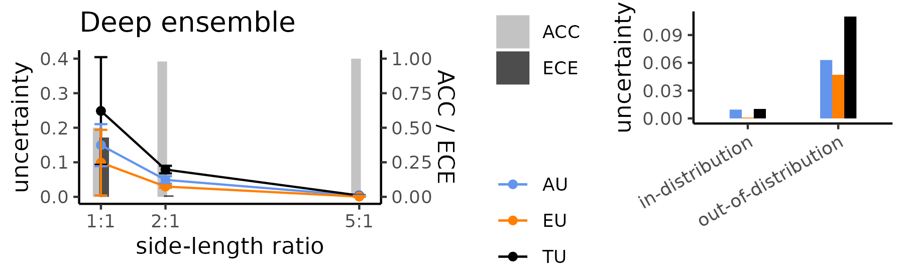
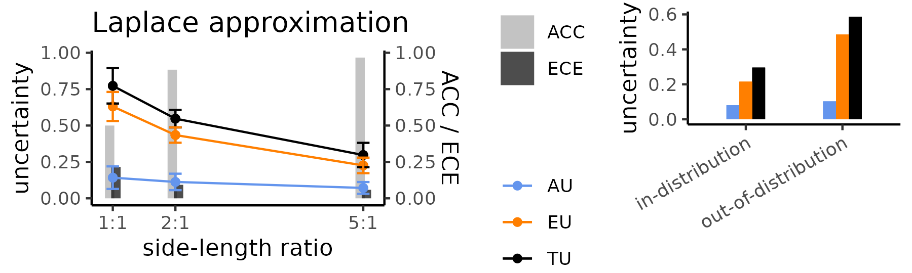
Figure 10: Entropy-based uncertainty for synthetic data with increasing class interpolation (left) and OOD detection (random polygons; right).

5.2.4 Discussion

Our experiments confirm empirically that the entropy-based uncertainty measures exhibit some – sometimes subtle – inconsistencies in different learning situations. While TU as a whole behaves fairly sensibly, the attribution to its aleatoric and epistemic components often appears implausible. We further identify very low levels of EU as a global pattern. That said, we also find that the design of the probabilistic learner used can affect the results considerably, even when predictive performance remains similar. In particular, deep ensembles draw from the opinions of various base learners when they estimate predictive uncertainty, as opposed to Laplace approximation, where a single base network determines uncertainty quantification. Consequently, the behavior of explicit ensembles also depends on the complexity of their base learners in that AU estimates decrease considerably when each ensemble member is granted more capacity (see supplementary material B.3). This relates to another insight relevant for this kind of empirical studies: reasoning about uncertainty estimates must always occur in conjunction with predictive accuracy and calibration, since we can hardly expect sensible uncertainty behavior when the learner fails on the basic underlying task. Numerous practical aspects thus interact to elicit or mitigate shortcomings of the discussed measures and warrant caution in interpreting any predictive uncertainty estimate one may obtain in practice. Worryingly, this becomes all the more important with limited data, a situation often encountered in, e.g., medical applications.

6 Concluding Remarks

Despite the common use of Shannon entropy, conditional entropy, and mutual information for the quantification of predictive uncertainty, we observed and empirically confirmed that these measures behave neither coherently nor always as expected. First, each of the measures itself can be criticized for (the lack of) certain properties. For example, we argued that mutual information is rather a measure of divergence than a measure of ignorance. Second, the discrepancy between (i) the ground-truth scenario concerning the true data-generating process with an objective ground-truth AU and zero EU, and (ii) the finite-sample setting in which AU is derived from (and hence depends on) subjective EU, leads to incoherencies and calls additivity of the decomposition into question. With this in mind, we encourage a critical assessment of the existing framework and cautious use of these measures.

When remaining committed to the basic (Bayesian) representational framework with second-order distributions for the epistemic part of uncertainty, an obvious alternative is to look for measures with better properties, and indeed, some proposals can be found in the recent literature (e.g., Sicking et al. [2020]). Another option is to change not only the measures for quantification, but also the underlying representation, for example by moving beyond classical probability. In fact, the suitability of probability distributions to represent ignorance in the sense of a lack of knowledge has been questioned by various scholars [Dubois et al., 1996], who advocate the use of generalized, more expressive uncertainty formalisms. In particular, it has been argued that the uniform distribution is not a suitable representation of complete ignorance, as it fails to distinguish the epistemic state of zero knowledge and the state of perfect information, where the learner knows that all outcomes are equiprobable. Indeed, the averaging over conditional entropies, which is part of the problems with the aleatoric component, is arguably meaningful in the latter case but much less so in the former. Seen from this perspective, one may indeed wonder whether classical probability is the right paradigm for modeling the epistemic part. On the other side, measuring uncertainty and disaggregating total predictive uncertainty into its aleatoric and epistemic components do not necessarily become simpler for generalized formalisms [Hüllermeier et al., 2022]. Clearly, we are not yet at the end of the path toward a truly meaningful uncertainty representation and quantification.

Appendix A Experimental Details

In the following, we list the most important training configurations used to generate our results. The full experimental code is hosted in a public repository.

Software

Our codebase is written in Python. It chiefly relies on the PyTorch [Paszke et al., 2019], PyTorch Lightning [Lightning AI, 2023], Laplace Redux [Daxberger et al., 2021], and scikit-learn [Pedregosa et al., 2011] libraries.

Datasets

The real-world computer vision tasks are CIFAR10 [Krizhevsky, 2009] and MNIST [LeCun et al., 1998]. Both contain ten balanced classes. We further synthesize rectangles (white-on-black), where the class label is determined by whether height $>$ width or vice versa, and random non-convex polygons (white-on-black) with 3–5 vertices. These datasets comprise 60k (10k) training (test) samples. The tabular classification problem is created via scikit-learn’s make_classification function, using two features (and four classes. Here, we generate 6k (1k) training (test) samples.

Base learners

Our probabilistic classifiers all combine some base learners into an explicit (deep ensemble, random forest) or implicit (Laplace approximation) ensemble. We train EfficientNet-B7 (approx. 64m parameters; Tan and Le [2019]) for CIFAR10 and a small convolutional network (three convolutional layers with ReLU activation; approx. 62k parameters) for MNIST and the rectangle/polygon images. In the tabular classification problem, we use a random forest with a maximum tree depth of ten as well as single-hidden-layer MLPs with a hidden layer size of ten, adopting the default parameters from scikit-learn unless stated otherwise. Ensemble size is set to $M=10$.

Training Configurations

We use an SGD optimizer (momentum 0.9), a learning rate schedule with cosine annealing, where the initial learning rate is set to $10^{-2}$, and weight decay ($5\times 10^{-4}$). Training runs for a maximum of 200 epochs at batch size 256 with early stopping if validation loss does not improve over five consecutive epochs (evaluated on a validation set containing 10% of the training data).

Appendix B Additional Results

B.1 Increasing Data Noise

Compared to the ensemble of MLPs, the random forest (Fig. 11) reacts in both uncertainty components when class overlap is increased.

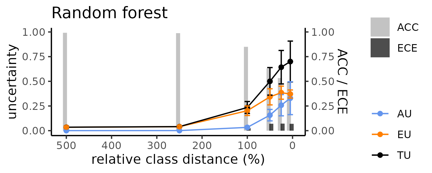
Figure 11: Entropy-based uncertainty for increasing class overlap (tabular data).

In order to simulate label noise, we randomly change classes for a varying share (1%–75%) of observations in the tabular classification task, leading to datasets as depicted in Fig. 12.

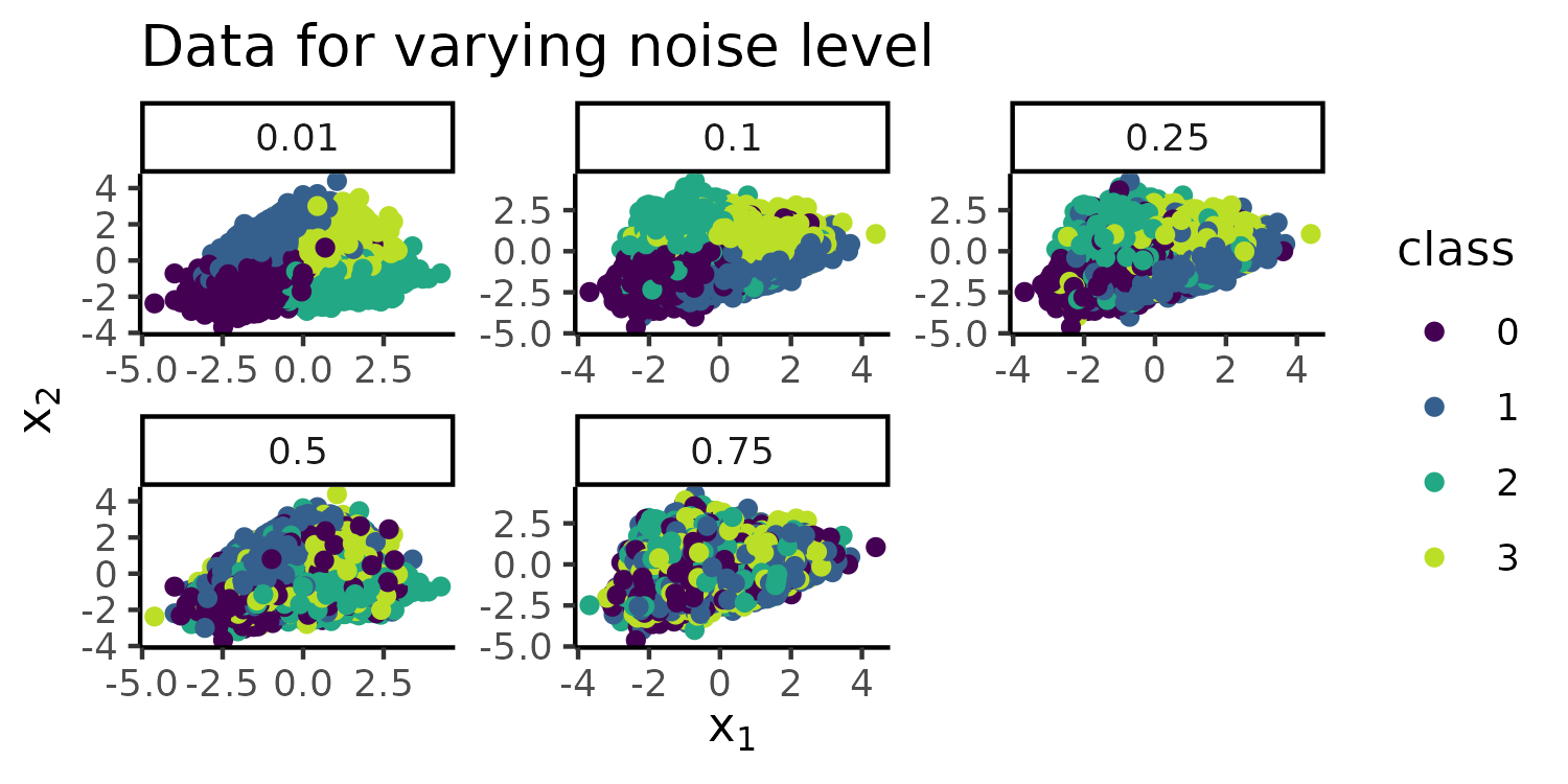
Figure 12: Tabular data with two features and four classes for increasing noise level.

Expected Behavior

AU picks up with increasing noise level. Since learner capacity remains fixed, it is reasonable to assume that EU also rises to some extent when the decision boundaries become more complex with mounting degree of dataset contamination.

Observed Behavior

As observed in the experiments modifying image resolution and class overlap, we find that AU duly increases for a rising noise level, though it remains moderate for the random forest even in the most extreme scenario (Fig. 13), where three out of four labels are assigned randomly. EU goes up slightly for the random forest, as presumed, but remains ultra-low for every value of the ablation with the MLP ensemble.

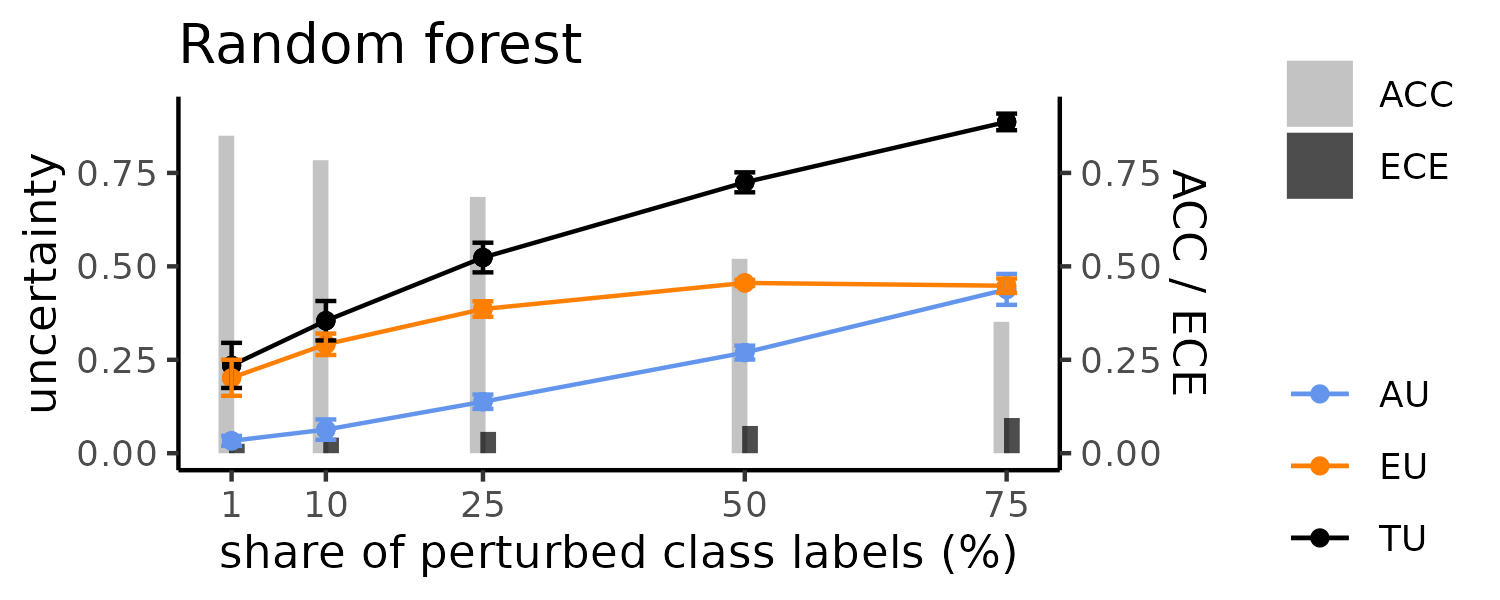
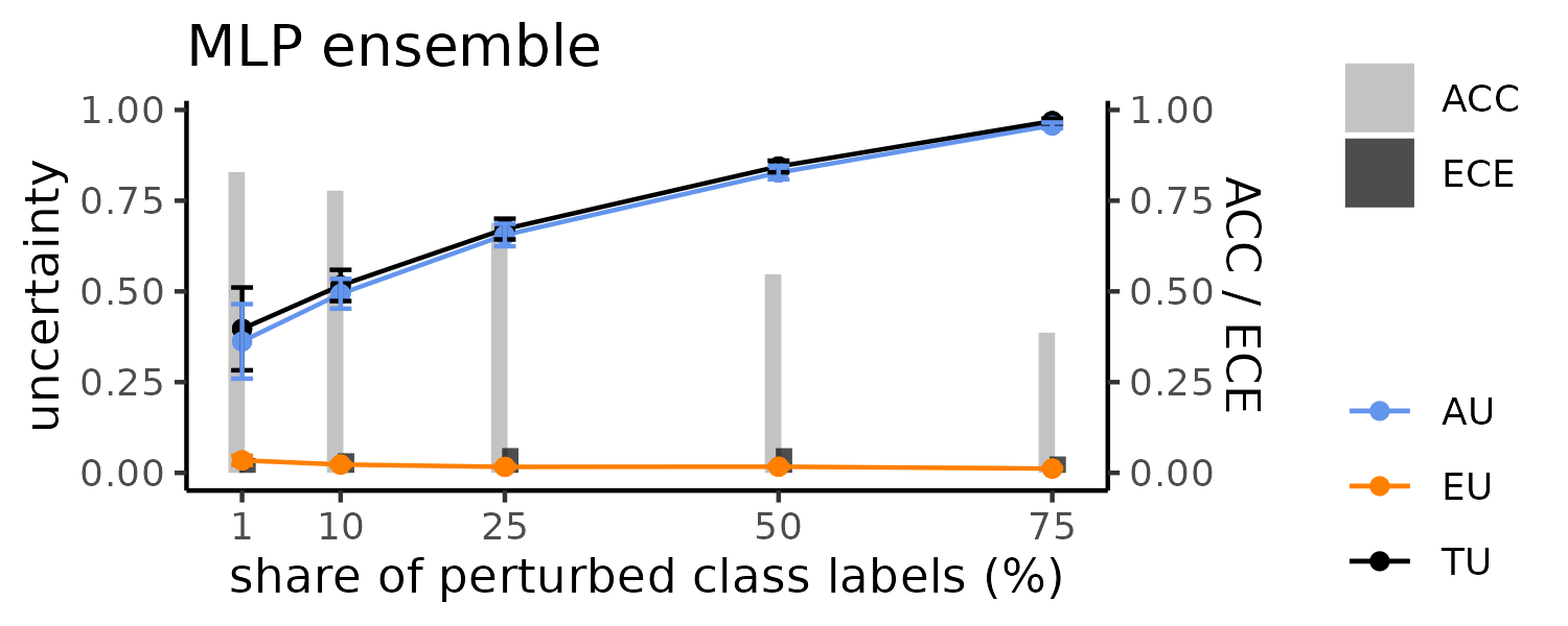
Figure 13: Entropy-based uncertainty for increasing label noise (tabular data).

B.2 Number of Ensemble Members

We study for the tabular classification problem how different ensemble sizes (2–50) affect the uncertainty estimates.

Expected Behavior

There should be no systematic pattern except for possible volatility for very small ensemble sizes, where the finite-ensemble estimator might have larger bias.

Observed Behavior

The results are indeed fairly stable for different values of $M$ (Fig. 14). Again, the overall levels of reported uncertainty differ considerably between the learners.

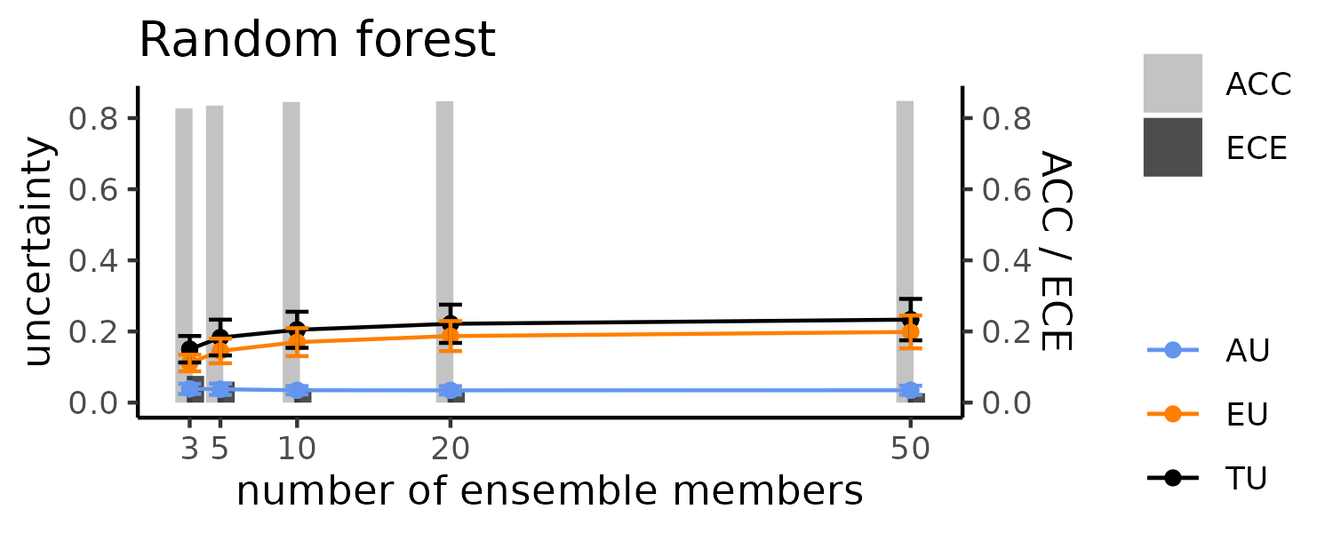
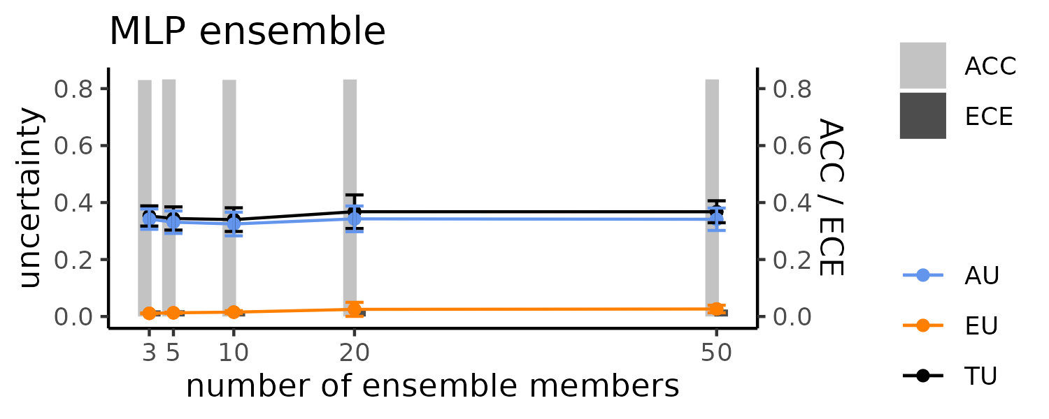
Figure 14: Entropy-based uncertainty for increasing number of ensemble members (tabular data).

We also compute the uncertainty measures for the computer vision tasks, where such large ensembles are prohibitively expensive, that result from using $M=5$. Tables 1–8 show the uncertainty values as an average over all possible five-member ensembles that can be constructed from the ten original predictions (we can compute this ex post since ensemble size does not affect training for either of the used probabilistic learners: deep ensembles are trained in parallel with no shared loss propagation, and Laplace approximation is an inherently ex-post approach anyway). The results are quite robust here as well (with some exceptions for the particularly noisy settings, such as 1% sample size).

B.3 Base Learner Complexity

Lastly, we investigate the effect of changing the base learner’s capacity in the random forest and ensemble of MLPs. As a a proxy for capacity, we use maximum tree depth and hidden-layer size, respectively.

Expected Behavior

Initially, AU should decrease when base learners get more capacity so they can fit more varied distributions, express their confidence more adequately and achieve better calibration. Similarly, the additional complexity might result in higher EU because the base learners have more freedom for disagreement.

Observed Behavior

We find that AU indeed reduces considerably for more complex base learners (Fig. 15), especially for the random forest, which appears to overstate AU when the base learners are very simple (resulting in high calibration error). The strong effect is quite striking and might be overlooked as performance is relatively stable, again underlining that accuracy, calibration and uncertainty must be considered jointly. EU, on the other hand, does not change much – apparently, relation between capacity and reported AU is quite consistent across base learners and does not provoke more conflict when the ensemble members obtain more freedom.

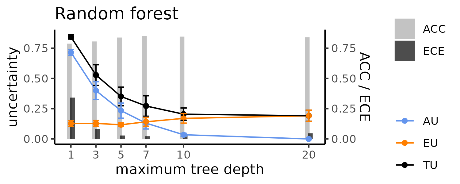
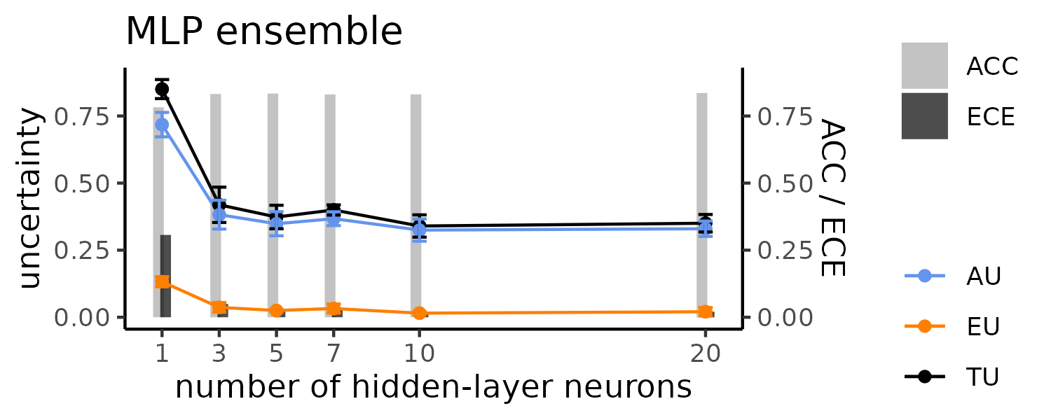
Figure 15: Increasing base learner complexity

Table 1: Results for sample size with ensemble of $M=5$. Mean and standard deviation are obtained by aggregating over all possible ensembles of size five that can be sampled from the ten predictions of the original experiment.

Experiment	Case	Probabilistic learner	Dataset	Measure	Mean	Standard deviation	$M=10$
sample size	1	Laplace approximation	MNIST	TU	0.5918	0.0451	0.7754
sample size	1	Laplace approximation	MNIST	AU	0.0091	0.0012	0.0091
sample size	1	Laplace approximation	MNIST	EU	0.5827	0.0449	0.7663
sample size	2	Laplace approximation	MNIST	TU	0.5794	0.0436	0.7419
sample size	2	Laplace approximation	MNIST	AU	0.0386	0.0037	0.0388
sample size	2	Laplace approximation	MNIST	EU	0.5408	0.0416	0.7031
sample size	5	Laplace approximation	MNIST	TU	0.5370	0.0416	0.6716
sample size	5	Laplace approximation	MNIST	AU	0.0631	0.0053	0.0634
sample size	5	Laplace approximation	MNIST	EU	0.4738	0.0391	0.6083
sample size	10	Laplace approximation	MNIST	TU	0.4578	0.0364	0.5760
sample size	10	Laplace approximation	MNIST	AU	0.0447	0.0039	0.0449
sample size	10	Laplace approximation	MNIST	EU	0.4131	0.0341	0.5311
sample size	50	Laplace approximation	MNIST	TU	0.1756	0.0247	0.2147
sample size	50	Laplace approximation	MNIST	AU	0.0354	0.0033	0.0355
sample size	50	Laplace approximation	MNIST	EU	0.1402	0.0221	0.1791
sample size	100	Laplace approximation	MNIST	TU	0.0793	0.0116	0.0947
sample size	100	Laplace approximation	MNIST	AU	0.0223	0.0022	0.0224
sample size	100	Laplace approximation	MNIST	EU	0.0570	0.0096	0.0723

Table 2: Results for sample size with ensemble of $M=5$. Mean and standard deviation are obtained by aggregating over all possible ensembles of size five that can be sampled from the ten predictions of the original experiment.

Experiment	Case	Probabilistic learner	Dataset	Measure	Mean	Standard deviation	$M=10$
sample size	1	deep ensemble	MNIST	TU	0.0487	0.0110	0.0518
sample size	1	deep ensemble	MNIST	AU	0.0343	0.0065	0.0344
sample size	1	deep ensemble	MNIST	EU	0.0144	0.0049	0.0174
sample size	2	deep ensemble	MNIST	TU	0.0381	0.0042	0.0404
sample size	2	deep ensemble	MNIST	AU	0.0257	0.0032	0.0258
sample size	2	deep ensemble	MNIST	EU	0.0124	0.0016	0.0146
sample size	5	deep ensemble	MNIST	TU	0.0212	0.0017	0.0223
sample size	5	deep ensemble	MNIST	AU	0.0152	0.0012	0.0153
sample size	5	deep ensemble	MNIST	EU	0.0060	0.0011	0.0070
sample size	10	deep ensemble	MNIST	TU	0.0137	0.0011	0.0144
sample size	10	deep ensemble	MNIST	AU	0.0098	0.0007	0.0099
sample size	10	deep ensemble	MNIST	EU	0.0039	0.0007	0.0045
sample size	50	deep ensemble	MNIST	TU	0.0082	0.0007	0.0087
sample size	50	deep ensemble	MNIST	AU	0.0051	0.0004	0.0051
sample size	50	deep ensemble	MNIST	EU	0.0031	0.0004	0.0036
sample size	100	deep ensemble	MNIST	TU	0.0067	0.0008	0.0072
sample size	100	deep ensemble	MNIST	AU	0.0042	0.0004	0.0042
sample size	100	deep ensemble	MNIST	EU	0.0025	0.0004	0.0030

Table 3: Results for sample size with ensemble of $M=5$. Mean and standard deviation are obtained by aggregating over all possible ensembles of size five that can be sampled from the ten predictions of the original experiment.

Experiment	Case	Probabilistic learner	Dataset	Measure	Mean	Standard deviation	$M=10$
sample size	1	Laplace approximation	CIFAR10	TU	0.8171	0.0629	0.8507
sample size	1	Laplace approximation	CIFAR10	AU	0.6339	0.0587	0.6364
sample size	1	Laplace approximation	CIFAR10	EU	0.1832	0.0290	0.2143
sample size	2	Laplace approximation	CIFAR10	TU	0.5742	0.0368	0.6030
sample size	2	Laplace approximation	CIFAR10	AU	0.4337	0.0277	0.4354
sample size	2	Laplace approximation	CIFAR10	EU	0.1405	0.0092	0.1676
sample size	5	Laplace approximation	CIFAR10	TU	0.3823	0.0247	0.4114
sample size	5	Laplace approximation	CIFAR10	AU	0.2449	0.0158	0.2459
sample size	5	Laplace approximation	CIFAR10	EU	0.1374	0.0089	0.1655
sample size	10	Laplace approximation	CIFAR10	TU	0.3000	0.0199	0.3268
sample size	10	Laplace approximation	CIFAR10	AU	0.1776	0.0117	0.1783
sample size	10	Laplace approximation	CIFAR10	EU	0.1224	0.0083	0.1485
sample size	50	Laplace approximation	CIFAR10	TU	0.1327	0.0089	0.1460
sample size	50	Laplace approximation	CIFAR10	AU	0.0724	0.0048	0.0727
sample size	50	Laplace approximation	CIFAR10	EU	0.0603	0.0043	0.0733
sample size	100	Laplace approximation	CIFAR10	TU	0.0690	0.0047	0.0736
sample size	100	Laplace approximation	CIFAR10	AU	0.0460	0.0030	0.0461
sample size	100	Laplace approximation	CIFAR10	EU	0.0231	0.0018	0.0275

Table 4: Results for sample size with ensemble of $M=5$. Mean and standard deviation are obtained by aggregating over all possible ensembles of size five that can be sampled from the ten predictions of the original experiment.

Experiment	Case	Probabilistic learner	Dataset	Measure	Mean	Standard deviation	$M=10$
sample size	1	deep ensemble	CIFAR10	TU	0.9022	0.0715	0.9425
sample size	1	deep ensemble	CIFAR10	AU	0.7073	0.1223	0.7100
sample size	1	deep ensemble	CIFAR10	EU	0.1949	0.0770	0.2324
sample size	2	deep ensemble	CIFAR10	TU	0.7189	0.0652	0.7750
sample size	2	deep ensemble	CIFAR10	AU	0.4410	0.0676	0.4428
sample size	2	deep ensemble	CIFAR10	EU	0.2778	0.0404	0.3322
sample size	5	deep ensemble	CIFAR10	TU	0.4204	0.0273	0.4523
sample size	5	deep ensemble	CIFAR10	AU	0.2519	0.0173	0.2529
sample size	5	deep ensemble	CIFAR10	EU	0.1685	0.0113	0.1995
sample size	10	deep ensemble	CIFAR10	TU	0.2826	0.0183	0.3072
sample size	10	deep ensemble	CIFAR10	AU	0.1545	0.0106	0.1551
sample size	10	deep ensemble	CIFAR10	EU	0.1281	0.0082	0.1521
sample size	50	deep ensemble	CIFAR10	TU	0.1318	0.0131	0.1458
sample size	50	deep ensemble	CIFAR10	AU	0.0617	0.0076	0.0620
sample size	50	deep ensemble	CIFAR10	EU	0.0701	0.0057	0.0838
sample size	100	deep ensemble	CIFAR10	TU	0.1064	0.0176	0.1187
sample size	100	deep ensemble	CIFAR10	AU	0.0480	0.0101	0.0482
sample size	100	deep ensemble	CIFAR10	EU	0.0585	0.0078	0.0706

Table 5: Results for image resolution with ensemble of $M=5$. Mean and standard deviation are obtained by aggregating over all possible ensembles of size five that can be sampled from the ten predictions of the original experiment.

Experiment	Case	Probabilistic learner	Dataset	Measure	Mean	Standard deviation	$M=10$
image resolution	5	Laplace approximation	MNIST	TU	0.7660	0.0571	0.8540
image resolution	5	Laplace approximation	MNIST	AU	0.3781	0.0387	0.3796
image resolution	5	Laplace approximation	MNIST	EU	0.3879	0.0418	0.4744
image resolution	10	Laplace approximation	MNIST	TU	0.6475	0.0463	0.6996
image resolution	10	Laplace approximation	MNIST	AU	0.3847	0.0348	0.3862
image resolution	10	Laplace approximation	MNIST	EU	0.2628	0.0317	0.3134
image resolution	25	Laplace approximation	MNIST	TU	0.1149	0.0099	0.1261
image resolution	25	Laplace approximation	MNIST	AU	0.0634	0.0048	0.0636
image resolution	25	Laplace approximation	MNIST	EU	0.0516	0.0057	0.0624
image resolution	50	Laplace approximation	MNIST	TU	0.0787	0.0087	0.0923
image resolution	50	Laplace approximation	MNIST	AU	0.0259	0.0024	0.0260
image resolution	50	Laplace approximation	MNIST	EU	0.0528	0.0065	0.0663
image resolution	100	Laplace approximation	MNIST	TU	0.0703	0.0108	0.0833
image resolution	100	Laplace approximation	MNIST	AU	0.0212	0.0024	0.0213
image resolution	100	Laplace approximation	MNIST	EU	0.0491	0.0085	0.0620

Table 6: Results for image resolution with ensemble of $M=5$. Mean and standard deviation are obtained by aggregating over all possible ensembles of size five that can be sampled from the ten predictions of the original experiment.

Experiment	Case	Probabilistic learner	Dataset	Measure	Mean	Standard deviation	$M=10$
image resolution	5	deep ensemble	MNIST	TU	0.7635	0.0487	0.7672
image resolution	5	deep ensemble	MNIST	AU	0.7585	0.0484	0.7615
image resolution	5	deep ensemble	MNIST	EU	0.0050	0.0008	0.0056
image resolution	10	deep ensemble	MNIST	TU	0.5378	0.0350	0.5413
image resolution	10	deep ensemble	MNIST	AU	0.5272	0.0344	0.5292
image resolution	10	deep ensemble	MNIST	EU	0.0107	0.0013	0.0121
image resolution	25	deep ensemble	MNIST	TU	0.0519	0.0039	0.0537
image resolution	25	deep ensemble	MNIST	AU	0.0421	0.0030	0.0423
image resolution	25	deep ensemble	MNIST	EU	0.0098	0.0012	0.0114
image resolution	50	deep ensemble	MNIST	TU	0.0088	0.0008	0.0093
image resolution	50	deep ensemble	MNIST	AU	0.0058	0.0004	0.0059
image resolution	50	deep ensemble	MNIST	EU	0.0030	0.0004	0.0035
image resolution	100	deep ensemble	MNIST	TU	0.0074	0.0006	0.0079
image resolution	100	deep ensemble	MNIST	AU	0.0046	0.0004	0.0046
image resolution	100	deep ensemble	MNIST	EU	0.0028	0.0003	0.0033

Table 7: Results for image resolution with ensemble of $M=5$. Mean and standard deviation are obtained by aggregating over all possible ensembles of size five that can be sampled from the ten predictions of the original experiment.

Experiment	Case	Probabilistic learner	Dataset	Measure	Mean	Standard deviation	$M=10$
image resolution	5	Laplace approximation	CIFAR10	TU	0.7137	0.0451	0.7171
image resolution	5	Laplace approximation	CIFAR10	AU	0.7093	0.0448	0.7122
image resolution	5	Laplace approximation	CIFAR10	EU	0.0043	0.0003	0.0049
image resolution	10	Laplace approximation	CIFAR10	TU	0.2676	0.0169	0.2697
image resolution	10	Laplace approximation	CIFAR10	AU	0.2593	0.0164	0.2603
image resolution	10	Laplace approximation	CIFAR10	EU	0.0083	0.0005	0.0095
image resolution	25	Laplace approximation	CIFAR10	TU	0.1151	0.0073	0.1176
image resolution	25	Laplace approximation	CIFAR10	AU	0.1007	0.0064	0.1011
image resolution	25	Laplace approximation	CIFAR10	EU	0.0144	0.0010	0.0165
image resolution	50	Laplace approximation	CIFAR10	TU	0.0835	0.0055	0.0890
image resolution	50	Laplace approximation	CIFAR10	AU	0.0545	0.0036	0.0547
image resolution	50	Laplace approximation	CIFAR10	EU	0.0290	0.0021	0.0343
image resolution	100	Laplace approximation	CIFAR10	TU	0.0690	0.0047	0.0736
image resolution	100	Laplace approximation	CIFAR10	AU	0.0460	0.0030	0.0461
image resolution	100	Laplace approximation	CIFAR10	EU	0.0231	0.0018	0.0275

Table 8: Results for image resolution with ensemble of $M=5$. Mean and standard deviation are obtained by aggregating over all possible ensembles of size five that can be sampled from the ten predictions of the original experiment.

Experiment	Case	Probabilistic learner	Dataset	Measure	Mean	Standard deviation	$M=10$
image resolution	5	deep ensemble	CIFAR10	TU	0.7351	0.0467	0.7425
image resolution	5	deep ensemble	CIFAR10	AU	0.7012	0.0446	0.7040
image resolution	5	deep ensemble	CIFAR10	EU	0.0339	0.0027	0.0386
image resolution	10	deep ensemble	CIFAR10	TU	0.3727	0.0248	0.3900
image resolution	10	deep ensemble	CIFAR10	AU	0.2752	0.0197	0.2763
image resolution	10	deep ensemble	CIFAR10	EU	0.0975	0.0067	0.1137
image resolution	25	deep ensemble	CIFAR10	TU	0.2084	0.0187	0.2265
image resolution	25	deep ensemble	CIFAR10	AU	0.1134	0.0126	0.1138
image resolution	25	deep ensemble	CIFAR10	EU	0.0950	0.0068	0.1127
image resolution	50	deep ensemble	CIFAR10	TU	0.1174	0.0088	0.1302
image resolution	50	deep ensemble	CIFAR10	AU	0.0527	0.0045	0.0529
image resolution	50	deep ensemble	CIFAR10	EU	0.0648	0.0046	0.0773
image resolution	100	deep ensemble	CIFAR10	TU	0.1045	0.0137	0.1160
image resolution	100	deep ensemble	CIFAR10	AU	0.0480	0.0084	0.0482
image resolution	100	deep ensemble	CIFAR10	EU	0.0565	0.0055	0.0679