Picking Up Speed: Continuous-Time Lidar-Only Odometry using Doppler Velocity Measurements

Abstract

Frequency-Modulated Continuous-Wave (FMCW) lidar is a recently emerging technology that additionally enables per-return instantaneous relative radial velocity measurements via the Doppler effect. In this letter, we present the first continuous-time lidar-only odometry algorithm using these Doppler velocity measurements from an FMCW lidar to aid odometry in geometrically degenerate environments. We apply an existing continuous-time framework that efficiently estimates the vehicle trajectory using Gaussian process regression to compensate for motion distortion due to the scanning-while-moving nature of any mechanically actuated lidar (FMCW and non-FMCW). We evaluate our proposed algorithm on several real-world datasets, including publicly available ones and datasets we collected. Our algorithm outperforms the only existing method that also uses Doppler velocity measurements, and we study difficult conditions where including this extra information greatly improves performance. We additionally demonstrate state-of-the-art performance of lidar-only odometry with and without using Doppler velocity measurements in nominal conditions. Code for this project can be found at: https://github.com/utiasASRL/steam_icp.

I Introduction

Multi-beam lidars have become a common addition to the sensor suite of an autonomous vehicle. Estimation algorithms to handle the long-range 3D measurements (i.e., point clouds) produced by these sensors have also matured, and are capable of producing highly accurate motion estimates, often at a sub-decimeter level of accuracy for localization [1].

Lidar motion estimation performs exceptionally when there exists sufficient geometric structure in the surroundings to uniquely constrain all six degrees of freedom of the vehicle pose. In contrast, even the best estimators will struggle and even fail in geometrically degenerate environments. Long tunnels, highways with a barren landscape, and bridges are typical examples of extreme conditions where prior knowledge of the vehicle kinematics is insufficient to compensate for the lack of geometric information. A common solution in such situations is to rely on an additional sensor such as an Inertial Measurement Unit (IMU) [2, 3].

Frequency-Modulated Continuous Wave (FMCW) lidar is a recently emerging technology [4, 5] that provides a promising alternative solution for geometrically degenerate environments. While capable of producing dense point clouds comparable to a typical time-of-flight lidar, FMCW lidars also measure the relative velocity between each measured point along the radial direction via the Doppler effect, which we call a Doppler velocity measurement. Figure 1 depicts an example lidar frame colored by the Doppler velocity of each point. Hexsel et al. [6] recently showed that these Doppler velocity measurements are beneficial for lidar odometry in an Iterative Closest Point (ICP)-based algorithm.

Figure 1: An example lidar frame from the Aeva Aeries I FMCW Lidar colored by the measured relative radial velocity (i.e., Doppler velocity). Vehicles driving in the same direction are colored in magenta as they have the same velocity as the ego-vehicle, while vehicles driving in the opposite direction are in red. They can be clearly distinguished from the underlying static scene. Our proposed algorithm uses the relative radial velocity with respect to the static scene to aid odometry. Moving objects are naturally rejected by our algorithm using robust estimation techniques.

In this letter, we improve upon the existing work [6] by incorporating the Doppler velocity measurements in a continuous-time estimation framework. Continuous-time estimation allows for each measurement to be associated with its actual time of acquisition, avoiding the need for an IMU to correct the motion distortion of a lidar frame due to the scanning-while-moving nature of mechanically actuated lidars. Similar to [6], we present a Doppler velocity factor that can be applied in conjunction with the usual point-to-plane factor for frame-to-map alignment. However, our proposed factor differs from theirs in that it is applied to the vehicle’s body-centric velocity as opposed to pose since body-centric velocity is also part of our estimated state. We evaluate our lidar odometry algorithm on several real-world datasets, including publicly available ones collected using a non-FMCW lidar and datasets we collected using an FMCW lidar. Through our evaluation, we demonstrate overall state-of-the-art lidar-only odometry performance with and without using Doppler velocity measurements under both nominal and geometrically degenerate conditions.

II Related Work

Lidar motion estimation typically adopts a point cloud registration approach using a variant of ICP [7, 8]. Most lidar motion estimation pipelines can be divided into a data processing front-end and a state estimation back-end [9].

The front-end processes the raw lidar frames, which includes keypoint/feature extraction, global/local map building, and data association. LOAM [2] extracts edge and plane features and matches them via nearest-neighbor association. SuMa [10] matches raw frames to a surfel map using projective data association. Recently, Vizzo et al. [11] introduced a triangle mesh map representation and a ray-casting-based point-to-mesh association approach. Other alternatives have been proposed in [12, 13, 14, 15, 16, 17, 18], though we do not discuss them in detail in the interest of space.

The back-end leverages the processed data to estimate the vehicle state over time, seen as the vehicle trajectory. Existing approaches are different in how they formulate and estimate the trajectory. Discrete-time estimators formulate a trajectory where there is a temporal state (i.e., marginal) that corresponds to the acquisition time of every measurement. However, typical multi-beam lidars are mechanically actuated and produce thousands of measurements for every lidar frame. Consequently, each measurement may have a unique timestamp. Even after preprocessing into sparser keypoints, it is often not feasible to have a discrete state estimate at each measurement time. One option is to correct for the motion of each frame using an additional sensor such as an IMU [2, 3].

Alternatively, the vehicle trajectory can be estimated as a continuous function of time. The most straightforward approach is to apply linear interpolation between discrete states [19, 2, 20]. However, using linear interpolation between poses restricts the trajectory to have a piece-wise constant velocity, which cannot accurately represent trajectories undergoing high-frequency changes in velocity. Dellenbach et al. [21] address this limitation by allowing the vehicle poses to be discontinuous between lidar frames, trading trajectory smoothness for a closer representation. Another option for higher representational power without losing smoothness is to represent the trajectory using temporal basis functions [22, 23]. Referred to as a parametric methods, the trajectory is parameterized by the associated basis-function weights and has been demonstrated several times for lidar motion estimation using B-splines [24, 25, 26, 27].

Nonparametric methods instead estimate the continuous-time trajectory as a Gaussian process (GP) [28]. Barfoot et al. [29] demonstrated that through careful selection of the underlying GP prior and a Markovian state, we can benefit from the usual sparsity exploited in discrete-time estimation. Anderson and Barfoot [30] extended this idea for trajectory estimation in $SE(3)$. A desirable feature of their approach is that the GP prior is made to be physically motivated (e.g., white noise on acceleration). Lidar motion estimation has been demonstrated several times using various GP priors [31, 32, 33, 1].

All works discussed thus far consider lidars that only produce point clouds (optionally with intensity information). Advancements in FMCW technology have enabled a new type of lidar, i.e., the Aeva Aeries I FMCW Lidar [34], that can additionally measure the relative radial velocity (Doppler velocity) of each point. Hexsel et al. [6] presented an ICP-based algorithm that uses the Doppler velocity measurements and demonstrated improved performance in environments with insufficient geometric structure.

The Aeva Aeries I FMCW Lidar is mechanically actuated, similar to existing multi-beam lidars. Hexsel et al. [6] applied a discrete-time estimator, which requires the lidar frames to be corrected for motion beforehand using an IMU. We improve upon their work by formulating the back-end estimator using GP regression in $SE(3)$ [30]. Although the GP regression approach has been applied to lidar odometry before [31, 32, 33, 1], the benefits of including Doppler velocity measurements have not been demonstrated. Compared to the work of Hexsel et al. [6], we demonstrate state-of-the-art performance in lidar odometry without using additional sensors.

Furthermore, the FMCW technology can also be applied to radars, and there has been some work using an FMCW radar for motion estimation [35, 36]. Both Kellner et al. [35] and Vivet et al. [36] use the Doppler velocity measurements from an FMCW radar to estimate the velocity of the ego-vehicle, which is the same as what they are used for in this work.

III Methodology

Our lidar odometry algorithm adopts the conventional ICP-based frame-to-map approach while incorporating Doppler velocity measurements in a sliding-window implementation.

III-A Data Processing Front-End

We follow the approach of Dellenbach et al. [21]. Keypoints are extracted from each lidar frame via voxel grid downsampling. We use a grid size of 1.5m and keep one random point in each voxel. Our local map is a point cloud accumulated from the most recent frames and cropped to be within 100m of the latest estimate of the vehicle after each frame update. The local map is stored in a sparse voxel grid structure with a 1m grid size and a maximum of 20 points per voxel. We use point-to-plane ICP for frame-to-map matching. Each frame point is associated with a map point via nearest-neighbor association, and the corresponding plane normal is computed by applying Principle Component Analysis (PCA) to the 20 closest neighbors of the associated map point.

III-B Trajectory Estimation Back-End

Figure 2: This diagram shows the states and factors involved in our sliding-window estimation with an example window size of two. We query the trajectory states at the acquisition time of each keypoint in each lidar frame. The motion prior factor $\phi_{\text{mp}}$ connects neighboring trajectory states. The point-to-plane factor $\phi_{\text{p2p}}$ requires local map information while the Doppler velocity factor $\phi_{\text{dv}}$ does not. For computational efficiency, we implement this sliding-window estimation by introducing one estimated state at the end of each lidar frame and using GP interpolation to obtain states at other measurement times. This way, motion prior factors between interpolated and estimated/interpolated states are merged into factors between estimated states. Point-to-plane and Doppler velocity factors applied to interpolated states depend on the adjacent estimated states. Past states falling outside the window are marginalized and no longer updated.

Notation: We denote $\underrightarrow{\boldsymbol{\mathcal{F}}}_{i}$ to be the inertial reference frame, $\underrightarrow{\boldsymbol{\mathcal{F}}}_{v}$ to be the vehicle reference frame, and $\underrightarrow{\boldsymbol{\mathcal{F}}}_{\ell}$ to be the lidar reference frame. Let $\mathbf{T}_{vi}\in SE(3)$ be the inertial-to-vehicle transformation (i.e., the vehicle pose) and ${\boldsymbol{\varpi}}^{iv}_{v}=\begin{bmatrix}{{\boldsymbol{\nu}}^{iv}_{v}}^{T}&{{\boldsymbol{\omega}}^{iv}_{v}}^{T}\end{bmatrix}^{T}\in\mathbb{R}^{6}$ be the vehicle body-centric velocity where ${\boldsymbol{\nu}}^{iv}_{v}$ and ${\boldsymbol{\omega}}^{iv}_{v}$ are translational and rotational velocities, respectively. Furthermore, let $\mathbf{T}_{\ell v}$ be the fixed vehicle-to-lidar transformation assuming the lidar is rigidly mounted on the vehicle, $\mathbf{q}$ be a homogeneous point from a lidar frame (expressed in $\underrightarrow{\boldsymbol{\mathcal{F}}}_{\ell}$), and $\mathbf{p}$ be a homogeneous point in the local map (expressed in $\underrightarrow{\boldsymbol{\mathcal{F}}}_{i}$).

We follow previous work [30] to represent a continuous-time trajectory as a Gaussian process (GP). Our trajectory is $\mathbf{x}(t)=\{\mathbf{T}_{vi}(t),{\boldsymbol{\varpi}}^{iv}_{v}(t)\}$. We use the White-Noise-on-Acceleration (WNOA) motion prior

$$\begin{split}\dot{\mathbf{T}}_{vi}(t)&={\boldsymbol{\varpi}}^{iv}_{v}(t)^{\wedge}\mathbf{T}_{vi}(t),\\ \dot{{\boldsymbol{\varpi}}}^{iv}_{v}(t)&=\mathbf{w}(t),\quad\mathbf{w}(t)\sim\mathcal{GP}(\mathbf{0},\mathbf{Q}_{c}\delta(t-\tau)),\end{split}$$ (1)

where $\mathbf{w}(t)\in\mathbb{R}^{6}$ is a zero-mean, white-noise GP. The prior is applied in a piecewise fashion across an underlying discrete trajectory of pose-velocity state pairs, $\mathbf{x}_{k}$, each corresponding to the end time of the $k^{\text{th}}$ lidar frame. Note that the period of the $k^{\text{th}}$ frame lies between $\mathbf{x}_{k-1}$ and $\mathbf{x}_{k}$. For a keypoint $\mathbf{q}_{j}$ with acquisition time $t_{j}$ where $t_{k-1}<t_{j}<t_{k}$, we associate it to an interpolated state $\mathbf{x}(t_{j})$ that depends on $\mathbf{x}_{k-1}$ and $\mathbf{x}_{k}$ through GP interpolation. Interpolation is done efficiently through our choice of motion prior and Markovian state [30].

We jointly align the most recent five frames to the local map in a sliding window by optimizing for the states $\mathbf{x}_{k-5}$ to $\mathbf{x}_{k}$. Figure 2 illustrates the states and factors in our problem. We refer readers to Anderson and Barfoot [30] for details on the motion prior factor and discuss the measurement factors below.

III-B1 Point-to-Plane Factor

The point-to-plane factor is

$$\phi_{\text{p2p}} = \rho\left(\sqrt{\alpha^{4}\;e^{2}_{\text{p2p}}}\right),$$ (2)

$$e_{\text{p2p}} = \mathbf{n}^{T}\mathbf{D}\left(\mathbf{p}-\mathbf{T}_{vi}(t)^{-1}\mathbf{T}_{\ell v}^{-1}\mathbf{q}\right),$$ (3)

with $\mathbf{q}$ measured at time $t$ and $\mathbf{T}_{vi}(t)$ being the vehicle pose queried from the trajectory. $\mathbf{p}$ is the nearest neighbor of $\mathbf{q}$ in the local map, $\mathbf{n}$ is the surface normal of $\mathbf{p}$, and $\alpha=(\sigma_{2}-\sigma_{3})/\sigma_{1}$ [21, 38] is a heuristic weight to favour planar neighborhoods. $\mathbf{D}$ is a constant projection that removes the fourth homogeneous element. $\rho(\cdot)$ is a robust cost function chosen to be Cauchy with $c=0.5$ [39], and we discard any measurement resulting in $e_{\text{p2p}}\geq 0.5\text{m}$.

Figure 3: This diagram provides a graphical illustration of the Doppler velocity error term derivation. $\underrightarrow{\boldsymbol{\mathcal{F}}}_{i}$, $\underrightarrow{\boldsymbol{\mathcal{F}}}_{v}$, and $\underrightarrow{\boldsymbol{\mathcal{F}}}_{\ell}$ are the inertial, vehicle, and lidar reference frames, respectively. $\mathbf{q}$ and $\dot{\mathbf{q}}$ are the measured point position and velocity expressed in $\underrightarrow{\boldsymbol{\mathcal{F}}}_{\ell}$, respectively. $\mathbf{d}$ is a unit vector along the direction of $\mathbf{q}$, and $\widetilde{\dot{r}}$ is the relative radial velocity according to ${\boldsymbol{\varpi}}^{i\ell}_{\ell}=\begin{bmatrix}{{\boldsymbol{\nu}}^{i\ell}_{\ell}}^{T}&{{\boldsymbol{\omega}}^{i\ell}_{\ell}}^{T}\end{bmatrix}^{T}$. See Section III-B for the expression of $\mathbf{d}$ and $\widetilde{\dot{r}}$.

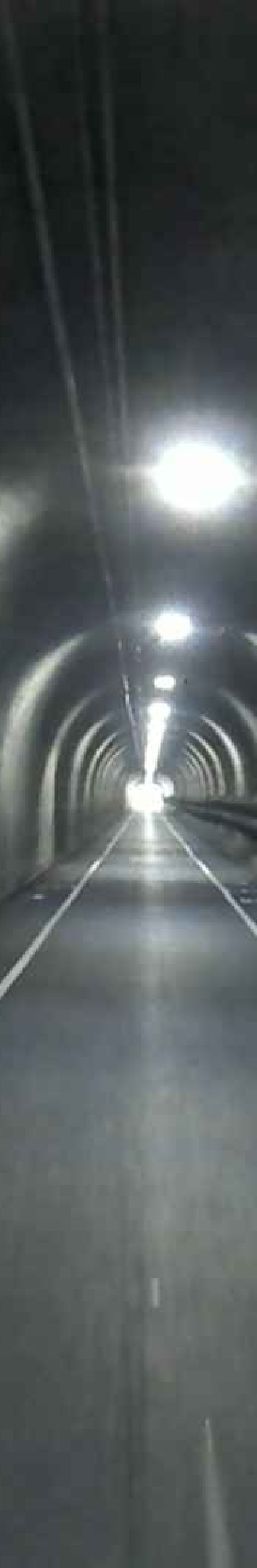
(a) Baker-Barry Tunnel

(b) Robin Williams Tunnel

(c) Ontario Highway 404

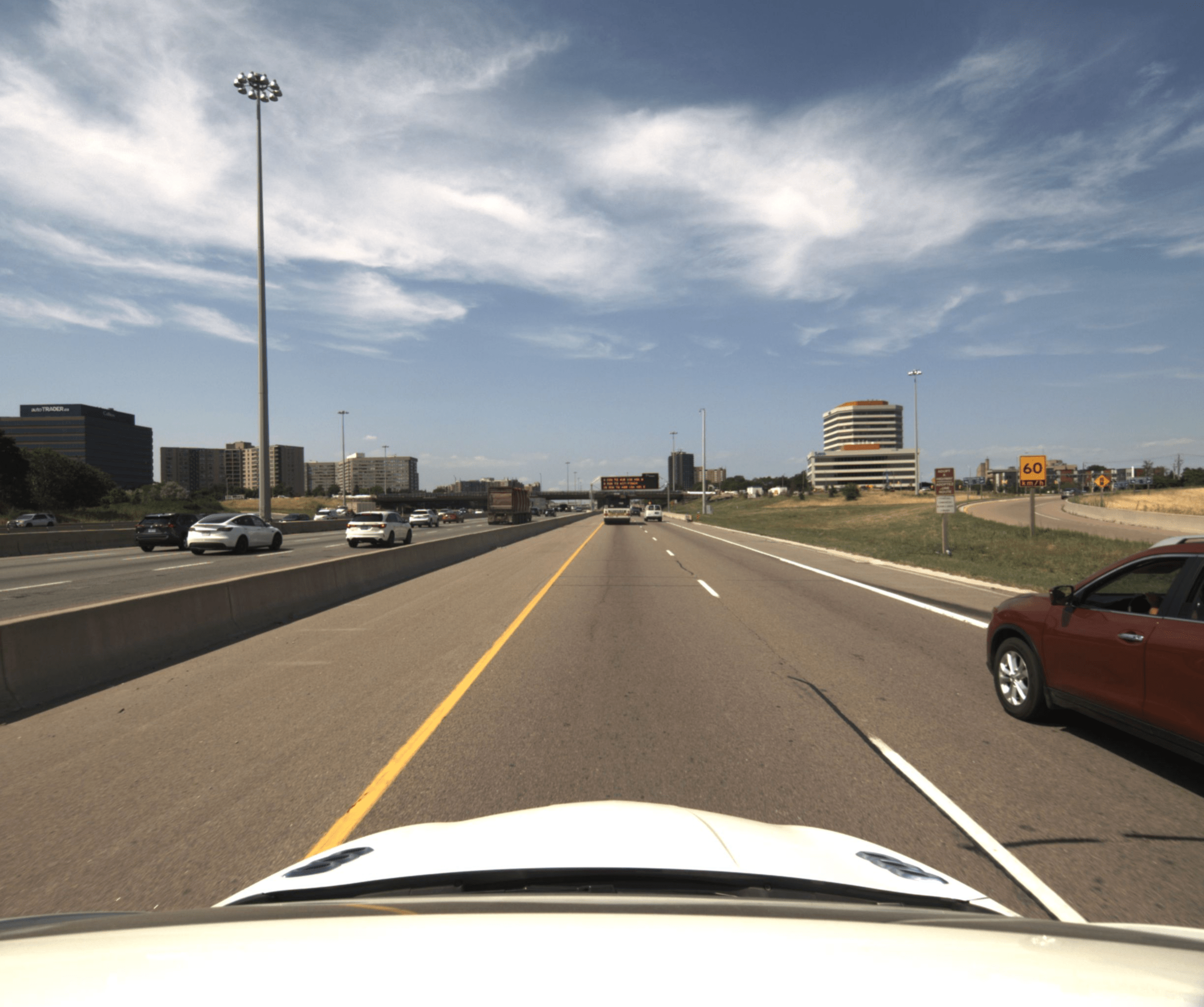
(d) Ontario Highway 427

Figure 4: Representative scenes in the Aeva dataset. The straight tunnels (LABEL:sub@subfig:bb) and (LABEL:sub@subfig:rw) have poor geometric structure to constrain the vehicle motion in the longitudinal direction. The Ontario highway sequences have moderate geometric structure from buildings and vegetation by the side of the highway.

III-B2 Doppler Velocity Factor

The Doppler velocity factor is

$$\phi_{\text{dv}} = \rho\left(\sqrt{\beta\;e^{2}_{\text{dv}}}\right),$$ (4)

$$e_{\text{dv}} = \dot{r}-\dfrac{\mathbf{q}^{T}\mathbf{D}^{T}}{(\mathbf{q}^{T}\mathbf{D}^{T}\mathbf{D}\mathbf{q})^{1/2}}\mathbf{D}\mathbf{q}^{\odot}{\boldsymbol{\mathcal{T}}}_{\ell v}{\boldsymbol{\varpi}}^{iv}_{v}(t),$$ (5)

where ${\boldsymbol{\varpi}}^{iv}_{v}(t)$ is the vehicle body-centric velocity queried at $t$, $\mathbf{D}$ is the same projection as above, $\dot{r}$ is the Doppler velocity measurement associated with $\mathbf{q}$ measured at time $t$, ${\boldsymbol{\mathcal{T}}}_{\ell v}=\text{Ad}\left(\mathbf{T}_{\ell v}\right)$ is the adjoint matrix of $\mathbf{T}_{\ell v}$, and the $(\cdot)^{\odot}$ operator converts a homogeneous point to a $4\times 6$ matrix, as defined in [37, p.246]. $\beta=0.1$ is a constant heuristic weight and $\rho(\cdot)$ is again the Cauchy robust cost function with $c=0.05$ [39]. We dicard any measurement resulting in $e_{\text{dv}}\geq 2\text{m/s}$.

To derive our error term (5), we first define $\dot{\mathbf{q}}$ and $\dot{\mathbf{q}}_{i}$ to be $\mathbf{q}$’s velocity expressed in the lidar and inertial reference frame, respectively. Applying the transport theorem,

$$\dot{\mathbf{q}}_{i}=\mathbf{T}_{i\ell}(t)\left(\dot{\mathbf{q}}-{{\boldsymbol{\varpi}}^{i\ell}_{\ell}}(t)^{\wedge}\mathbf{q}\right).$$ (6)

Assuming $\mathbf{q}$ is static in the inertial frame such that $\dot{\mathbf{q}}_{i}=0$, we can rearrange (6) to be (see $SE(3)$ identities in [37])

$$\dot{\mathbf{q}} = {{\boldsymbol{\varpi}}^{i\ell}_{\ell}}(t)^{\wedge}\mathbf{q}$$ (7)

$$= \mathbf{q}^{\odot}{\boldsymbol{\varpi}}^{i\ell}_{\ell}(t)$$

$$= \mathbf{q}^{\odot}{\boldsymbol{\mathcal{T}}}_{\ell v}{\boldsymbol{\varpi}}^{iv}_{v}(t),$$

where (7) relates the point velocity $\dot{\mathbf{q}}$ to the body-centric velocity component of our trajectory state ${\boldsymbol{\varpi}}^{iv}_{v}$. Next, we project $\dot{\mathbf{q}}$ onto $\mathbf{q}$ to obtain the predicted Doppler velocity:

$$\widetilde{\dot{r}}=\underbrace{\dfrac{\mathbf{q}^{T}\mathbf{D}^{T}}{\left(\mathbf{q}^{T}\mathbf{D}^{T}\mathbf{D}\mathbf{q}\right)^{1/2}}}_{\text{Projection }\mathbf{d}}\mathbf{D}\mathbf{q}^{\odot}{\boldsymbol{\mathcal{T}}}_{\ell v}{\boldsymbol{\varpi}}^{iv}_{v}(t).$$ (8)

Finally, taking the difference between the predicted and measured relative radial velocity gives the error function $e_{\text{dv}}$ in (5). This derivation is graphically illustrated in Figure 3.

Figure 5: Our platform, Boreas, is previously used to collect the Boreas dataset [40] and additionally equipped with an Aeva Aeries I FMCW Lidar [34] for use in this work.

TABLE I: Aeva Dataset Statistics

Seq. #	Location	Length [m]	Num. of Frames	Geometric Structure
00	Baker-Barry Tunnel (Empty)	860	837	Poor
01	Baker-Barry Tunnel (Vehicles)	907	658	Poor
02	Robin Williams Tunnel	689	301	Poor
03	Brisbane Lagoon Freeway	4942	1762	Poor
04	Ontario Highway 7	8876	6343	Moderate
05	Ontario Highway 407	7836	4734	Moderate
06	Don Valley Parkway	10310	5083	Moderate
07	Ontario Highway 427	7238	4012	Moderate

TABLE II: Quantitative results on KITTI-raw/360 dataset using KITTI RTE metric. The average is computed over all segments of all sequences as in [21]. Note that CT-ICP optimizes one lidar frame at a time, while our algorithm optimizes multiple frames in a sliding window. For a fair comparison, we evaluate our algorithm using the estimated poses at the front of the window (i.e., newest timestamp).

KITTI-raw	00	01	02	03 (NA)	04	05	06	07	08	09	10	AVG
CT-ICP [21]	0.51	0.81	0.55	-	0.43	0.27	0.28	0.35	0.80	0.47	0.49	0.55
STEAM-ICP (Ours)	0.49	0.65	0.50	-	0.38	0.26	0.28	0.32	0.81	0.46	0.53	0.52
KITTI-360	00	01 (NA)	02	03	04	05	06	07	08 (NA)	09	10	AVG
CT-ICP [21]	0.41	-	0.38	0.34	0.65	0.39	0.42	0.34	-	0.45	0.69	0.45
STEAM-ICP (Ours)	0.41	-	0.38	0.48	0.69	0.40	0.43	0.60	-	0.35	0.73	0.45

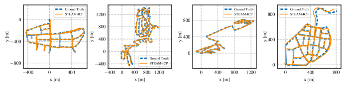
Figure 6: Trajectories estimated by STEAM-ICP from the longest four sequences (over 10000 frames) in KITTI-360 dataset: sequence 00 (11501 frames), 02 (19231 frames), 04 (11400 frames), and 09 (13955 frames).

At this point, we highlight the characteristics of our Doppler velocity factor. Firstly, the factor does not require the local map. Secondly, the rotational velocity of the lidar frame ${\boldsymbol{\omega}}_{\ell}^{i\ell}$ is unfortunately not observable. Finally, by having the vehicle’s body-centric velocity as part of the state, the Doppler velocity measurement is incorporated directly into our estimator without further approximations or assumptions. While the first two characteristics have been observed by Hexsel et al. [6], the last one is unique to our formulation. Hexsel et al. [6] derived a relation between Doppler velocity and vehicle pose using a constant-velocity approximation within the period of each frame, which is not needed in our formulation.

We treat sliding-window estimation as a factor-graph optimization problem and solve it iteratively using Gauss-Newton with Iteratively Reweighted Least Squares (IRLS) [41]. Rather than naively dropping states out of the sliding window, we explicitly marginalize out each old state. Each new state is initialized based on the GP extrapolation of our motion prior (i.e., constant velocity). The point-to-plane association of keypoints in the latest frame and the plane normals are re-computed after every five Gauss-Newton iterations.

IV Experiments

IV-A Datasets

We demonstrate our method and make comparisons to existing work on several real-world data sequences, which we categorize into two datasets: KITTI-raw/360 and Aeva. All data sequences provide accurate pose estimates from a GNSS-INS system for evaluation.

IV-A1 KITTI-raw/360 dataset

contains 19 sequences of raw lidar frames from the publicly available KITTI dataset [42] and its successor KITTI-360 [43]. The lidar used in this dataset is a Velodyne HDL-64, which is not an FMCW lidar. The sequences in this dataset were collected from urban/suburban environments and are rich in geometric structure for lidar motion estimation. We apply our estimator to the variation of the dataset made available by Dellenbach et al. [21].

IV-A2 Aeva dataset

contains 8 sequences of lidar frames from an Aeva Aeries I FMCW Lidar that produces Doppler velocity measurements. Aeva Aeries I FMCW Lidar has a horizontal field-of-view of $120^{\circ}$, a vertical field-of-view of $30^{\circ}$, a 300m maximum operating range, a Doppler velocity measurement precision of 3cm/s, and a sampling rate of 10Hz.

Sequences 00-03 are relatively short sequences purposely collected in environments with poor geometric structure (e.g., tunnels, freeways), which have been used in previous work [6], but required an additional IMU to correct for the scanning-while-moving nature of the sensor. Sequences 04-07 are longer sequences collected using our data collection platform, Boreas (Figure 5), on Toronto, Ontario highways with moderate geometric structure. Table I has a summary of the dataset statistics, and Figure 4 shows some representative scenes.

TABLE III: Quantitative results on Aeva dataset using both KITTI RTE and Frame-to-Frame RTE metrics. Note that all algorithms (including Doppler-ICP) are evaluated using motion-distorted frames. We exclude the first 60 frames of each sequence from evaluation because the vehicle does not start at zero velocity in these sequences, which causes the local map to be initialized from motion-distorted frames. Results of Seq. 04-07 (Range-Limited) were obtained by limiting the range of the lidar frames to 40m.

	KITTI RTE [%]					Frame-to-Frame RTE [m]
Sequences 00-03	00	01	02	03	AVG	00	01	02	03	AVG
Doppler-ICP [6]	1.66	2.60	1.03	1.72	1.80	0.0246	0.0254	0.0380	0.0494	0.0402
CT-ICP [21]	2.83	12.26	9.11	1.54	3.35	0.0401	0.3753	0.2446	0.0801	0.1827
STEAM-ICP (Ours)	2.28	12.86	22.74	2.10	4.16	0.0541	0.4134	0.6076	0.2892	0.3180
STEAM-DICP (Ours)	2.35	2.60	0.74	1.70	1.88	0.0180	0.0211	0.0299	0.0362	0.0299
Sequences 04-07	04	05	06	07	AVG	04	05	06	07	AVG
Doppler-ICP [6]	3.86	2.81	2.13	2.93	3.00	0.0864	0.0485	0.0140	0.2355	0.1181
CT-ICP [21]	0.34	0.34	0.41	0.48	0.38	0.0194	0.0202	0.0198	0.0216	0.0202
STEAM-ICP (Ours)	0.38	0.29	0.36	0.36	0.35	0.0211	0.0250	0.0230	0.0298	0.0244
STEAM-DICP (Ours)	0.33	0.46	0.30	0.37	0.36	0.0064	0.0119	0.0081	0.0201	0.0119
Seq. 04-07 (Range-Limited)	04	05	06	07	AVG	04	05	06	07	AVG
Doppler-ICP [6]	13.73	6.29	2.72	6.95	7.96	0.2555	0.1679	0.0198	0.4047	0.2444
CT-ICP [21]	10.90	56.44	66.64	5.39	33.87	0.0857	1.9122	1.8926	0.0637	1.3279
STEAM-ICP (Ours)	67.48	3.48	2.57	3.99	24.50	1.6030	0.1107	0.0644	0.1778	0.9056
STEAM-DICP (Ours)	2.25	3.11	2.28	2.27	2.44	0.0173	0.0337	0.0211	0.0453	0.0297

Figure 7: This figure shows a comparison of Frame-to-Frame RTE between STEAM-ICP and STEAM-DICP on the Robin Williams Tunnel sequence (left), the corresponding trajectories versus ground truth (middle), and the point cloud map built from STEAM-DICP (right). Due to the poor geometric structure in the longitudinal direction, STEAM-ICP under-estimates the length of the trajectory inside the tunnel, while STEAM-DICP remains unaffected thanks to the correction from Doppler velocity measurements.

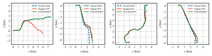
Figure 8: Trajectories estimated by STEAM-DICP and Doppler-ICP from sequences 04-07 in the Aeva dataset without limiting the range of the sensor. Doppler-ICP exhibits higher drifts due to using a frame-to-frame registration approach and not accounting for motion distortion.

IV-B Evaluation

We use the KITTI Relative Translation Error (KITTI RTE), which averages the translation error over path segments of lengths 100m to 800m in 100m intervals. For the Aeva dataset, we additionally include evaluation using the Frame-to-Frame Relative Translation Error (Frame-to-Frame RTE) metric [44], which was used in [6]. In the interest of space, we omit showing the rotation error in the main text since the translation error is where our comparisons differ the most. Interested readers can find our full evaluation results in our supplementary material [45].

We name the two variants of our algorithm using and not using the Doppler velocity measurements STEAM-DICP and STEAM-ICP, respectively, after the continuous-time trajectory estimation framework, STEAM, presented in [30].

On the KITTI-raw/360 dataset, we compare STEAM-ICP with CT-ICP [21]. CT-ICP, to the best of our knowledge, is the current state-of-the-art continuous-time lidar-only odometry algorithm. It achieves similar performance on the KITTI odometry benchmark as other state-of-the-art methods (e.g., LOAM [2], IMLS-SLAM [38], and MULLS [18]) using lidar frames without motion distortion and demonstrates better performance using lidar frames with motion distortion. On the Aeva dataset, we compare STEAM-DICP with STEAM-ICP, CT-ICP, and Doppler-ICP [6]. Note that Doppler-ICP is the only existing algorithm that also uses Doppler velocity measurements to aid lidar odometry.

IV-C Results

Table II shows quantitative results on the KITTI-raw/360 dataset. Compared to CT-ICP, our odometry achieves comparable performance, demonstrating that we are performing at state of the art using non-FMCW lidars (i.e., no Doppler velocity measurements). Example plots of the estimated trajectory are shown in Figure 6.

Quantitative results on the Aeva dataset are shown in Table III. On the difficult sequences with insufficient geometric structure (i.e., sequences 00-03), both CT-ICP and STEAM-ICP (i.e., methods that do not use Doppler velocity measurements) perform poorly. Figure 7 highlights the problem in sequence 02 (Robin Williams Tunnel), where we see that the Frame-to-Frame RTE for both CT-ICP and STEAM-ICP increases dramatically during the tunnel portion of the sequence.

On sequences with moderate geometric structure (i.e., sequences 04-07), methods that do not use the velocity measurements perform well. Doppler-ICP performs worse overall due to using a frame-to-frame approach (i.e., no accumulated local maps) and not accounting for the motion in each lidar frame. STEAM-DICP performs similarly to STEAM-ICP and CT-ICP, showing that the velocity measurements are not as impactful on sequences with sufficient geometry. However, we still see minor improvements in Frame-to-Frame RTE, suggesting that the velocity measurements overall help improve performance.

Another way to highlight the benefit of the Doppler velocity measurements is to limit the range of the lidar artificially. The majority of the distinctive structure in the environment is off-road and further away from the sensor, therefore limiting the range increases the difficulty for estimation. We see in the Range-Limited section of Table III that methods using the Doppler velocity measurements, Doppler-ICP and STEAM-DICP, are the most robust to this artificial increase in difficulty, with ours (STEAM-DICP) performing the best.

IV-D Implementation

We implemented our back-end (see Section III-B) for continuous-time trajectory estimation using an open-source C++ library, STEAM [30]. The front-end that processes the lidar data was made to be the same as CT-ICP by using the C++ library that the authors have made publicly available. We use the same parameters as CT-ICP for keypoint extraction, neighborhood search, normal estimation, and map building to maintain a fair comparison. Parameters of the trajectory estimation back-end were determined empirically.

Our implementation is currently not quite real-time capable, running at approximately 5Hz on the KITTI sequences and approximately 2Hz on the Aeva sequences after incorporating the Doppler velocity measurements. The current bottleneck is the processing of each motion prior and measurement factor in STEAM, which was designed with more focus on generalization rather than computational speed. We strongly believe that a real-time capable implementation can be achieved by implementing an estimator specific to our problem, e.g., by hardcoding Jacobian computations instead of relying on STEAM’s built-in automatic differentiation.

V Conclusions

In this letter, we presented a continuous-time lidar odometry algorithm leveraging the Doppler velocity measurements from an FMCW lidar to aid odometry. Our algorithm combines the lidar data processing front-end in [21] with our STEAM continuous-time estimator as the back-end, efficiently estimating the vehicle trajectory using GP regression. Through continuous-time estimation, our algorithm handles the motion distortion problem of mechanically actuated lidars. Incorporating the Doppler velocity information helps prevent odometry failures under geometrically degenerate conditions. By estimating vehicle pose and body-centric velocity, Doppler velocity measurements are incorporated directly into the estimator without further approximations or assumptions. Using both publicly available and our own datasets, we demonstrated state-of-the-art lidar odometry performance under nominal conditions with and without velocity information. On kilometer-scale highway sequences, we demonstrated superior performance over the only existing lidar odometry method that also uses Doppler velocity information under nominal and geometrically degenerate conditions.

There are multiple directions for future work to improve the proposed algorithm further. Currently, we apply robust cost functions to the point-to-plane error $e_{\text{p2p}}$ and the Doppler velocity error $e_{\text{dv}}$ individually for outlier rejection. Alternatively, one can apply a single robust cost function to $\begin{bmatrix}e_{\text{p2p}}&e_{\text{dv}}\end{bmatrix}^{T}$ to reject outliers using both sources of information (in the same spirit as the Dynamic Point Outlier Rejection scheme in [6]). The velocity measurements can also be used by the data processing front-end to segment and remove points from moving objects before data association (e.g., by using the method of [46]). In addition, one can replace the WNOA GP prior used in this work with the WNOJ prior [32] or the Singer prior [33], which have shown to improve lidar odometry in nominal conditions.

Supplementary Material

This supplementary material presents the full quantitative results on the Aeva dataset using both KITTI Relative Pose Error metric (Table IV) and Frame-to-Frame Relative Pose Error metric (Table V) [44]. Note again that all algorithms are evaluated using motion-distorted frames, and we exclude the first 60 frames of each sequence from evaluation. Results of Seq. 04-07 (Range-Limited) were obtained by limiting the range of the lidar frames to 40m.

Results of the translation error have been reported and discussed in the main text. Regarding the rotation error, we see that Doppler-ICP seems to do slightly better in rotation on the Frame-to-Frame metric. However, the overall difference between Doppler-ICP and STEAM-DICP is not significant, and our algorithm outperforms theirs on the KITTI metric, which averages rotation error over longer trajectory segments.

TABLE IV: Quantitative results on Aeva dataset using KITTI Relative Pose Error metric.

	Translation [%]					Rotation [deg/m]
Sequences 00-03	00	01	02	03	AVG	00	01	02	03	AVG
Doppler-ICP [6]	1.66	2.60	1.03	1.72	1.80	0.0330	0.0143	0.0335	0.0064	0.0122
CT-ICP [21]	2.83	12.26	9.11	1.54	3.35	0.0085	0.0148	0.0121	0.0038	0.0062
STEAM-ICP (Ours)	2.28	12.86	22.74	2.10	4.16	0.0078	0.0155	0.0124	0.0040	0.0063
STEAM-DICP (Ours)	2.35	2.60	0.74	1.70	1.88	0.0077	0.0166	0.0137	0.0040	0.0065
Sequences 04-07	04	05	06	07	AVG	04	05	06	07	AVG
Doppler-ICP [6]	3.86	2.81	2.13	2.93	3.00	0.0115	0.0104	0.0079	0.0060	0.0093
CT-ICP [21]	0.34	0.34	0.41	0.48	0.38	0.0010	0.0012	0.0014	0.0015	0.0012
STEAM-ICP (Ours)	0.38	0.29	0.36	0.36	0.35	0.0012	0.0009	0.0011	0.0012	0.0011
STEAM-DICP (Ours)	0.33	0.46	0.30	0.37	0.36	0.0010	0.0013	0.0009	0.0012	0.0011
Seq. 04-07 (Range-Limited)	04	05	06	07	AVG	04	05	06	07	AVG
Doppler-ICP [6]	13.73	6.29	2.72	6.95	7.96	0.0350	0.0224	0.0103	0.0113	0.0213
CT-ICP [21]	10.90	56.44	66.64	5.39	33.87	0.0315	0.2084	0.2239	0.0165	0.1158
STEAM-ICP (Ours)	67.48	3.48	2.57	3.99	24.50	0.1218	0.0087	0.0072	0.0076	0.0455
STEAM-DICP (Ours)	2.25	3.11	2.28	2.27	2.44	0.0062	0.0090	0.0069	0.0071	0.0072

TABLE V: Quantitative results on Aeva dataset using Frame-to-Frame Relative Pose Error metric.

	Translation [m]					Rotation [deg]
Sequences 00-03	00	01	02	03	AVG	00	01	02	03	AVG
Doppler-ICP [6]	0.0246	0.0254	0.0380	0.0494	0.0402	0.1357	0.1670	0.1655	0.0827	0.1163
CT-ICP [21]	0.0401	0.3753	0.2446	0.0801	0.1827	0.1907	0.2865	0.1593	0.1163	0.1675
STEAM-ICP (Ours)	0.0541	0.4134	0.6076	0.2892	0.3180	0.1322	0.1855	0.1503	0.1195	0.1366
STEAM-DICP (Ours)	0.0180	0.0211	0.0299	0.0362	0.0299	0.1384	0.1821	0.1475	0.1125	0.1336
Sequences 04-07	04	05	06	07	AVG	04	05	06	07	AVG
Doppler-ICP [6]	0.0864	0.0485	0.0140	0.2355	0.1181	0.0557	0.0453	0.0655	0.0559	0.0558
CT-ICP [21]	0.0194	0.0202	0.0198	0.0216	0.0202	0.0460	0.0401	0.0582	0.0501	0.0485
STEAM-ICP (Ours)	0.0211	0.0250	0.0230	0.0298	0.0244	0.0460	0.0410	0.0603	0.0489	0.0490
STEAM-DICP (Ours)	0.0064	0.0119	0.0081	0.0201	0.0119	0.0447	0.0391	0.0587	0.0474	0.0474
Seq. 04-07 (Range-Limited)	04	05	06	07	AVG	04	05	06	07	AVG
Doppler-ICP [6]	0.2555	0.1679	0.0198	0.4047	0.2444	0.0917	0.0673	0.0688	0.0609	0.0741
CT-ICP [21]	0.0857	1.9122	1.8926	0.0637	1.3279	0.1300	71.1626	77.2449	0.1086	36.2160
STEAM-ICP (Ours)	1.6030	0.1107	0.0644	0.1778	0.9056	0.8207	0.1058	0.1211	0.0944	0.3328
STEAM-DICP (Ours)	0.0173	0.0337	0.0211	0.0453	0.0297	0.0923	0.0844	0.1059	0.0852	0.0925

References

- [1] K. Burnett, Y. Wu, D. J. Yoon, A. P. Schoellig, and T. D. Barfoot, “Are we ready for radar to replace lidar in all-weather mapping and localization?” IEEE Robotics and Automation Letters, vol. 7, no. 4, pp. 10 328–10 335, 2022.
- [2] J. Zhang and S. Singh, “Low-drift and real-time lidar odometry and mapping,” vol. 41, no. 2, pp. 401–416, 2017.
- [3] H. Ye, Y. Chen, and M. Liu, “Tightly coupled 3d lidar inertial odometry and mapping,” in 2019 International Conference on Robotics and Automation (ICRA), 2019, pp. 3144–3150.
- [4] B. Behroozpour, P. A. M. Sandborn, M. C. Wu, and B. E. Boser, “Lidar system architectures and circuits,” IEEE Communications Magazine, vol. 55, no. 10, pp. 135–142, 2017.
- [5] S. Royo and M. Ballesta-Garcia, “An overview of lidar imaging systems for autonomous vehicles,” Applied Sciences, vol. 9, no. 19, 2019.
- [6] B. Hexsel, H. Vhavle, and Y. Chen, “DICP: Doppler Iterative Closest Point Algorithm,” in Proceedings of Robotics: Science and Systems, 2022.
- [7] P. Besl and N. D. McKay, “A method for registration of 3-d shapes,” IEEE Transactions on Pattern Analysis and Machine Intelligence, vol. 14, no. 2, pp. 239–256, 1992.
- [8] F. Pomerleau, F. Colas, and R. Siegwart, A Review of Point Cloud Registration Algorithms for Mobile Robotics, 2015.
- [9] C. Cadena, L. Carlone, H. Carrillo, Y. Latif, D. Scaramuzza, J. Neira, I. Reid, and J. J. Leonard, “Past, Present, and Future of Simultaneous Localization and Mapping: Toward the Robust-Perception Age,” vol. 32, no. 6, pp. 1309–1332, 2016.
- [10] J. Behley and C. Stachniss, “Efficient surfel-based slam using 3d laser range data in urban environments,” in Proceedings of Robotics: Science and Systems, 2018.
- [11] I. Vizzo, X. Chen, N. Chebrolu, J. Behley, and C. Stachniss, “Poisson surface reconstruction for lidar odometry and mapping,” in 2021 IEEE International Conference on Robotics and Automation (ICRA), 2021, pp. 5624–5630.
- [12] T. Shan and B. Englot, “Lego-loam: Lightweight and ground-optimized lidar odometry and mapping on variable terrain,” in 2018 IEEE/RSJ International Conference on Intelligent Robots and Systems (IROS), 2018, pp. 4758–4765.
- [13] X. Chen, A. Milioto, E. Palazzolo, P. Giguère, J. Behley, and C. Stachniss, “Suma++: Efficient lidar-based semantic slam,” in 2019 IEEE/RSJ International Conference on Intelligent Robots and Systems (IROS), 2019, pp. 4530–4537.
- [14] D. Kovalenko, M. Korobkin, and A. Minin, “Sensor aware lidar odometry,” in 2019 European Conference on Mobile Robots (ECMR), 2019, pp. 1–6.
- [15] J. Lin and F. Zhang, “Loam livox: A fast, robust, high-precision lidar odometry and mapping package for lidars of small fov,” in 2020 IEEE International Conference on Robotics and Automation (ICRA), 2020, pp. 3126–3131.
- [16] S. W. Chen, G. V. Nardari, E. S. Lee, C. Qu, X. Liu, R. A. F. Romero, and V. Kumar, “Sloam: Semantic lidar odometry and mapping for forest inventory,” IEEE Robotics and Automation Letters, vol. 5, no. 2, pp. 612–619, 2020.
- [17] X. Zheng and J. Zhu, “Efficient lidar odometry for autonomous driving,” IEEE Robotics and Automation Letters, vol. 6, no. 4, pp. 8458–8465, 2021.
- [18] Y. Pan, P. Xiao, Y. He, Z. Shao, and Z. Li, “Mulls: Versatile lidar slam via multi-metric linear least square,” in 2021 IEEE International Conference on Robotics and Automation (ICRA), 2021, pp. 11 633–11 640.
- [19] M. Bosse and R. Zlot, “Continuous 3d scan-matching with a spinning 2d laser,” in 2009 IEEE International Conference on Robotics and Automation, 2009, pp. 4312–4319.
- [20] C. Park, P. Moghadam, S. Kim, A. Elfes, C. Fookes, and S. Sridharan, “Elastic lidar fusion: Dense map-centric continuous-time slam,” in 2018 IEEE International Conference on Robotics and Automation (ICRA), 2018, pp. 1206–1213.
- [21] P. Dellenbach, J.-E. Deschaud, B. Jacquet, and F. G. Goulette, “Ct-icp: Real-time elastic lidar odometry with loop closure,” in 2022 International Conference on Robotics and Automation (ICRA), 2022, pp. 5580–5586.
- [22] P. Furgale, T. D. Barfoot, and G. Sibley, “Continuous-time batch estimation using temporal basis functions,” in 2012 IEEE International Conference on Robotics and Automation, 2012, pp. 2088–2095.
- [23] S. Anderson and T. D. Barfoot, “Towards relative continuous-time slam,” in 2013 IEEE International Conference on Robotics and Automation, 2013, pp. 1033–1040.
- [24] R. Zlot and M. Bosse, “Efficient Large-scale Three-dimensional Mobile Mapping for Underground Mines,” vol. 31, no. 5, pp. 758–779, 2014.
- [25] L. Kaul, R. Zlot, and M. Bosse, “Continuous-Time Three-Dimensional Mapping for Micro Aerial Vehicles with a Passively Actuated Rotating Laser Scanner,” vol. 33, no. 1, pp. 103–132, 2016.
- [26] H. Alismail, L. D. Baker, and B. Browning, “Continuous trajectory estimation for 3d slam from actuated lidar,” in 2014 IEEE International Conference on Robotics and Automation (ICRA), 2014, pp. 6096–6101.
- [27] D. Droeschel and S. Behnke, “Efficient continuous-time slam for 3d lidar-based online mapping,” in 2018 IEEE International Conference on Robotics and Automation (ICRA), 2018, pp. 5000–5007.
- [28] C. H. Tong, P. Furgale, and T. D. Barfoot, “Gaussian Process Gauss-Newton for non-parametric simultaneous localization and mapping,” vol. 32, no. 5, pp. 507–525, 2013.
- [29] T. Barfoot, C. Hay Tong, and S. Sarkka, “Batch Continuous-Time Trajectory Estimation as Exactly Sparse Gaussian Process Regression,” in Robotics: Science and Systems X, 2014.
- [30] S. Anderson and T. D. Barfoot, “Full steam ahead: Exactly sparse gaussian process regression for batch continuous-time trajectory estimation on se(3),” in 2015 IEEE/RSJ International Conference on Intelligent Robots and Systems (IROS), 2015, pp. 157–164.
- [31] T. Y. Tang, D. J. Yoon, F. Pomerleau, and T. D. Barfoot, “Learning a bias correction for lidar-only motion estimation,” in 2018 15th Conference on Computer and Robot Vision (CRV), 2018, pp. 166–173.
- [32] T. Y. Tang, D. J. Yoon, and T. D. Barfoot, “A white-noise-on-jerk motion prior for continuous-time trajectory estimation on se(3),” IEEE Robotics and Automation Letters, vol. 4, no. 2, pp. 594–601, 2019.
- [33] J. N. Wong, D. J. Yoon, A. P. Schoellig, and T. D. Barfoot, “A Data-Driven Motion Prior for Continuous-Time Trajectory Estimation on SE(3),” vol. 5, no. 2, pp. 1429–1436, 2020.
- [34] “Aeva Inc. Aeva Aeries I,” https://www.aeva.com/aeries-i/, accessed: 2022-08-19.
- [35] D. Kellner, M. Barjenbruch, J. Klappstein, J. Dickmann, and K. Dietmayer, “Instantaneous ego-motion estimation using doppler radar,” in 16th International IEEE Conference on Intelligent Transportation Systems (ITSC 2013), 2013, pp. 869–874.
- [36] D. Vivet, P. Checchin, and R. Chapuis, “Localization and mapping using only a rotating fmcw radar sensor,” Sensors, vol. 13, pp. 4527–4552, 2013.
- [37] T. D. Barfoot, State Estimation for Robotics, 2017.
- [38] J.-E. Deschaud, “Imls-slam: Scan-to-model matching based on 3d data,” in 2018 IEEE International Conference on Robotics and Automation (ICRA), 2018, pp. 2480–2485.
- [39] K. MacTavish and T. D. Barfoot, “At all costs: A comparison of robust cost functions for camera correspondence outliers,” in 2015 12th Conference on Computer and Robot Vision, 2015, pp. 62–69.
- [40] K. Burnett, D. J. Yoon, Y. Wu, A. Z. Li, H. Zhang, S. Lu, J. Qian, W.-K. Tseng, A. Lambert, K. Y. K. Leung, A. P. Schoellig, and T. D. Barfoot, “Boreas: A multi-season autonomous driving dataset,” arXiv:2203.10168, 2022.
- [41] P. W. Holland and R. E. Welsch, “Robust regression using iteratively reweighted least-squares,” Communications in Statistics - Theory and Methods, vol. 6, no. 9, pp. 813–827, 1977.
- [42] A. Geiger, P. Lenz, and R. Urtasun, “Are we ready for autonomous driving? the kitti vision benchmark suite,” in 2012 IEEE Conference on Computer Vision and Pattern Recognition, 2012, pp. 3354–3361.
- [43] J. Xie, M. Kiefel, M.-T. Sun, and A. Geiger, “Semantic instance annotation of street scenes by 3d to 2d label transfer,” in 2016 IEEE Conference on Computer Vision and Pattern Recognition (CVPR), 2016, pp. 3688–3697.
- [44] D. Prokhorov, D. Zhukov, O. Barinova, K. Anton, and A. Vorontsova, “Measuring robustness of visual slam,” in 2019 16th International Conference on Machine Vision Applications (MVA), 2019, pp. 1–6.
- [45] Y. Wu, D. J. Yoon, K. Burnett, S. Kammel, Y. Chen, H. Vhavle, and T. D. Barfoot, “Picking up speed: Continuous-time lidar-only odometry using doppler velocity measurements,” arXiv:2209.03304, 2022.
- [46] M. Guo, K. Zhong, and X. Wang, “Doppler velocity-based algorithm for clustering and velocity estimation of moving objects,” in 2022 7th International Conference on Automation, Control and Robotics Engineering (CACRE), 2022, pp. 216–222.