Classical information entropy of parton distribution functions and an application in finding gluon saturation

Abstract

Entropy or information is a fundamental quantity contained in a system in statistical mechanics and information theory. In this paper, a definition of classical information entropy of parton distribution functions is suggested. The extensive and supper-additive properties of the defined entropy are discussed. The concavity is also deduced for the defined entropy. As an example, the classical information entropy of the gluon distribution of the proton is presented. There are some particular features of the evolution of the information entropy in the saturating domain, which can be used in finding the signals of gluon saturation.

The hadrons are the composite particles made of quarks and gluons, with complex inner structures. The one-dimensional momentum distributions of quarks and gluons of a hadron are described with parton distribution functions (PDFs) in the infinite momentum frame Bjorken (1969); Feynman (1969); Bjorken and Paschos (1969); Gribov (1973). Thanks to the collinear factorization theorem Collins and Soper (1987); Collins et al. (1989); Sterman (1995), the PDFs are the universal quantities in different scattering processes involving the hadron at high energies. PDFs are of the nonperturbative origin in quantum chromodynamics (QCD) theory Yang and Mills (1954); Gross and Wilczek (1973); Politzer (1973). The PDFs at the high energy scale is connected with the nonperturbative dynamics at the low energy scale, which is peculiarly hard to be calculated. Nevertheless, PDFs can be well extracted from the experimental measurements of high-energy reactions, such as the analyses of PDFs done by CT14 Dulat et al. (2016) and NNPDF Ball et al. (2010, 2012). Nowadays, the extracted PDF data sets are an important tool for the calculations of high-energy processes involving hadrons and the simulations of high-energy hadron colliders or fixed-target experiments.

Entropy is an important quantity of a system in thermodynamics. The second law of thermodynamical physics says that the entropy can not be reduced during the spontaneous evolution of the system. According to the famous Boltzmann entropy $S=k_{\rm B}{\rm ln}W$, the entropy describes the disorder or complexity of the system at the microscopic level. Here $W$ denotes the number of microstates that correspond to the same macroscopic thermodynamic state. The most general formula in statistical mechanics is Gibbs entropy, as $S=-k_{\rm B}\sum p_{i}{\rm ln}(p_{i})$. The Gibbs entropy turns into the Boltzmann entropy if all the microstates have the same probability. The entropy decreases to zero for a perfectly sharp distribution. The defined entropy in statistical mechanics is the only entropy that is equivalent to the classical thermodynamic entropy.

The information entropy in information theory was introduced by C. Shannon, and it is defined as a measure of how much “choice” or “surprise” is involved in the measurement of a random variable Shannon (1948). It is a quantification of the expected amount of information conveyed by identifying the outcome of a random variable. The definition of Shannon entropy is similar in mathematical form to that of the Gibbs entropy. Actually, the Gibbs entropy can be seen as simply the amount of Shannon information needed to identify the microscopic state of the system, given its macroscopic descriptions. The information entropy is a useful tool. It provides an important criterion for setting up probability distributions on the basis of partial knowledge, which leads to the maximum-entropy estimate of statistical inference. The prescription to get the equilibrium distributions of statistical mechanics by maximizing the Gibbs entropy subject to some constraints resembles the maximum-entropy principle in statistical inference. E. Jaynes argued that the statistical mechanics can be taken as a form of statistical inference rather than as a physical theory of which the additional assumptions are not contained in the laws of mechanics (such as ergodicity) Jaynes (1957a, b).

Investigating the inner structure of a hadron in a statistical view is a novel approach. How to define an entropy of the inner constituents inside a hadron in terms of PDFs is an interesting question. The picture of the partons inside a hadron is “frozen” during the short time of measurement. In the deep inelastic scattering (DIS) process for determining the PDFs, the quarks probed by the high-energy virtual photon just resemble the free and real particles: no strongly interactions or collisions between partons, no appearing and no disappearing during the short detecting time. Thus, the definition of a classical entropy of the partons with PDFs is the primary motivation of this work.

The hadron PDFs are the parton number density distributions in the $x$-space. To study the classical information entropy of PDFs, a proper definition of the entropy should be made with any given density distribution. To ensure the extensive property of the classical entropy, I find, the definition of the classical information entropy can be given as,

$$\begin{split}&S\equiv-\left[\int f(x){\rm ln}(f(x))dx-N{\rm ln}(N)+\alpha N\right],\\ &N\equiv\int f(x)dx,\end{split}$$ (1)

where $f(x)$ is the given density distribution which describes a system and $\alpha$ is an arbitrary constant. With a simple calculation by this definition, one finds that the entropy of $k$ times copy of a system equals $k$ times the entropy of the system, which is written as,

$$\begin{split}S\left[kf(x)\right]=kS\left[f(x)\right].\end{split}$$ (2)

The extensity of the classical entropy is met. With the definition in Eq. (1), the supper-additive property of the entropy is given by,

$$\begin{split}S\left[f(x)+g(x)\right]\geq S\left[f(x)\right]+S\left[g(x)\right].\end{split}$$ (3)

The equality between $S\left[f(x)+g(x)\right]$ and $S\left[f(x)\right]+S\left[g(x)\right]$ happens only if $g(x)=kf(x)$. The detailed proof of the supper-additive property is given in the appendix. With the extensive and supper-additive properties, the concavity can be easily derived: $S[\sum_{i}\lambda_{i}f_{i}(x)]\geq\sum_{i}S[\lambda_{i}f_{i}(x)]=\sum_{i}\lambda_{i}S[f_{i}(x)]$.

In information theory, for a discrete random variable with probability $p_{i}$, the information entropy is defined as,

$$\begin{split}S=-\sum_{i}p_{i}{\rm ln}(p_{i}).\end{split}$$ (4)

Let us derive a proper definition of the information entropy for a continuous random variable $x$, based on the definition for discrete random variable. For any given density distribution $f(x)$, one can construct a probability density distribution $\hat{f}(x)$ by doing the normalization, as $\hat{f}(x)=f(x)/N$ and $N=\int f(x)dx$. Let us discretize the continuous random variable $x$ with tiny bin width $h$. If $h$ is small enough, one has the information entropy for the probability density distribution $\hat{f}(x)$ as,

$$\begin{split}S[\hat{f}(x)]=-\sum_{i}\hat{f}(x)h{\rm ln}\left(\hat{f}(x)h\right)\\ =-\sum_{i}\hat{f}(x){\rm ln}\left(\hat{f}(x)h\right)h\\ =-\int\hat{f}(x){\rm ln}\left(\hat{f}(x)h\right)dx.\end{split}$$ (5)

Replacing $\hat{f}(x)$ with $f(x)/N$, one has,

$$\begin{split}S[\hat{f}(x)]=-\int\hat{f}(x){\rm ln}\left(\hat{f}(x)h\right)dx\\ =-\int\frac{f(x)}{N}{\rm ln}\left(\frac{f(x)}{N}h\right)dx\\ =-\frac{1}{N}\left[\int f(x){\rm ln}(f(x))dx-\int f(x){\rm ln}(N)dx\right.\\ \left.+\int f(x){\rm ln}(h)dx\right]\\ =-\frac{1}{N}\left[\int f(x){\rm ln}(f(x))dx-N{\rm ln}(N)+N{\rm ln}(h)\right].\end{split}$$ (6)

With the assumption of extensive property, one gets,

$$\begin{split}S[f(x)]=NS[\hat{f}(x)]=\\ =-\left[\int f(x){\rm ln}(f(x))dx-N{\rm ln}(N)+N{\rm ln}(h)\right].\end{split}$$ (7)

One sees that ${\rm ln}(h)$ is actually the $\alpha$ parameter in Eq. (1). Since the density distribution $f(x)$ can be greater than 1 in some regions of $x$, the term “$-\int f(x){\rm ln}(f(x))dx$” in the definition can be a negative value. Therefore the term “$-N{\rm ln}(h)$” is important to make sure the entropy is positive, as long as $h$ is small enough. In the derivation of the entropy, $h$ should be a very small quantity so that the integral equals the summation (see Eq. (5)). In practice, $h$ should be much smaller than the resolution in a measurement.

Entropy is an essential tool to quantify the level of disorder of a system, or the amount of “missing” information needed to determine the microstate of the system given the macrostate. We know that a hadron is a complex system of many partons viewed by a probe at high energy. Therefore the entropy concept can be applied to the hadron, and it could be a useful quantity in characterizing the hadron structure.

The maximum entropy principle tells us that the system is at the maximum entropy for the intestable distributions. The maximum entropy method is successful in the study of valence quark distributions of proton Wang and Chen (2015). The valence quark distributions are determined at the input $Q_{0}^{2}$ scale where there are only three valence quarks, and the number of valence quarks at the scale is known and fixed. The information entropy for the maximum entropy method in Ref. Wang and Chen (2015) is defined as $-\int f(x){\rm ln}(f(x))dx$, which is different from the definition in this work. However, the entropy differences from the variations of distributions are exactly the same for the definitions in this work and in Ref. Wang and Chen (2015), for $N{\rm ln}(N)-N{\rm ln}(h)$ is a constant if the number of quarks does not change at the fixed $Q_{0}^{2}$ scale. In the determination of quark distributions with maximum entropy method, the entropy difference matters instead of the absolute value of the entropy. Therefore the valence quark distributions determined in Ref. Wang and Chen (2015) are still valid and the same with the new entropy definition in this work.

In this letter, an application of the defined information entropy is illustrated in the search of the gluon saturation in the proton. The idea of parton saturation is that the occupation numbers of partons in the light-cone wave function of a hadron do not grow rapidly and reach a limiting distribution at small $x$ below the saturation momentum $Q_{s}$, which was initiated in the study of parton-parton recombination effect from the inevitable quanta overlapping Gribov et al. (1983); Mueller and Qiu (1986); Mueller (1990, 1999); McLerran and Venugopalan (1994a, b, c). In theory, the gluon saturation is rigorously guaranteed with the Jalilian-Marian-Iancu-McLerran-Weigert-Leonidov-Kovner equation Balitsky (1996); Jalilian-Marian et al. (1997); Iancu et al. (2001a); Weigert (2002) and the saturation solution of the equation is called color glass condensate (CGC) Iancu et al. (2001a, b); Jalilian-Marian and Kovchegov (2006); Gelis et al. (2010). A much simple evolution equation which also gives the gluon saturation is the Balitsky-Kovchegov equation Balitsky (1997); Kovchegov (1999, 2000); Balitsky (2001) with the resummation of fan diagrams (two Pomerons merge into one Pomeron) added to the Balitsky-Fadin-Kuraev-Lipatov evolution Lipatov (1976); Kuraev et al. (1977); Balitsky and Lipatov (1978). The gluon saturation is not only of such an extraordinary behavior of gluons at high density, but also important to restore the unitarity upper bound in QCD theory Froissart (1961); Martin (1963).

In experiment, it is a crucial problem and an interesting subject to find the clear signals of gluon saturation in various kinds of reactions in $p$-$p$, $p$-$A$, $e$-$p$ and $e$-$A$ collisions. Tremendous efforts from many physicists have been made to uncover the obscure signal of saturation. The traditional observables in high energy collisions, such as the structure functions and the cross sections of diffractive and inclusive processes, support more or less the existence of gluon saturation (see a review Morreale and Salazar (2021)). For the past decade, the more promising methods of two-particle correlations are developed and suggested to identify the gluon saturation. These two-particle correlations include the azimuthal correlations of dijet, or dihadron, or lepton-jet productions in the inclusive or diffractive processes (see a recent article Tong et al. (2023) and the literatures therein). In this work we would like to suggest a new way to probe and identify the gluon saturation by the evolution pattern of the information entropy over the $Q^{2}$ scale.

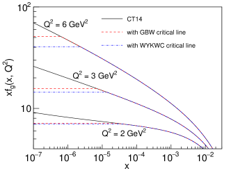
Figure 1: The gluon distributions at small $x$ from CT14 (solid curve) Dulat et al. (2016), the ideal saturation with GBW critical line (dashed curve) Golec-Biernat and Wusthoff (1998); Bartels et al. (2002); Kowalski and Teaney (2003), and the ideal saturation with WYKWC critical line (dash-dotted curve) Wang et al. (2021).

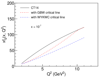
Figure 2: The evolution of gluon distribution at small $x$ in the relatively low $Q^{2}$ range, from CT14 PDF (solid curve) Dulat et al. (2016), the ideal saturation with GBW critical line (dashed curve) Golec-Biernat and Wusthoff (1998); Bartels et al. (2002); Kowalski and Teaney (2003), and the ideal saturation with WYKWC critical line (dash-dotted curve) Wang et al. (2021).

Before making a prediction for the entropy evolution in the saturation regime, let us first construct the saturated gluon distributions at small $x$ below the saturation momentum $Q_{s}$. An ideal form of strong gluon saturation is used for the calculations. According to some QCD models, the gluon density per unit area per unit rapidity $xg(x,Q^{2})$ is a constant in the strong saturation region, and the gluon density distribution $g(x,Q^{2})$ is proportional to $1/x$ Mueller and Qiu (1986); Mueller (1990); McLerran and Venugopalan (1994b). The saturated gluon distributions at small $x$ are displayed in Fig. 1, compared with the normal gluon distribution from CT14 analysis Dulat et al. (2016). The sharp and fast transition from nonsaturated distribution to saturated distribution is assumed across the critical line between the nonsaturating and saturating regimes. In this work, the critical lines from GBW’s Golec-Biernat and Wusthoff (1998); Bartels et al. (2002); Kowalski and Teaney (2003) and WYKWC’s Wang et al. (2021) parameterizations are taken. The WYKWC’s critical line is derived from an analytical solution of the simplified BK equation. The evolutions of the saturated gluon distribution and the CT14 gluon distribution in the low $Q^{2}$ range are present in Fig. 2. One sees that below the saturation momentum the saturated gluon distribution increases approximately linearly with $Q^{2}$. Actually this is consistent with the saturation model in the dipole picture Mueller (1990); Nikolaev and Zakharov (1991). The cross section $\sigma^{\rm\gamma^{*}p}=\sigma_{\rm T}+\sigma_{\rm L}$ is approximately a constant for small $Q^{2}$ in the saturation region Golec-Biernat and Wusthoff (1998) (the dipole size $r$ is almost always larger than the saturation scale $R_{0}(x)$ at small $x$). Eq. (8) expresses the connection between the $\gamma^{*}p$ cross section and the structure functions. It is clearly shown that the structure functions or the underlying parton distributions scale linearly with $Q^{2}$, in the saturating regime of small $x$ and small $Q^{2}$.

$$\begin{split}F_{\rm T,L}(x,Q^{2})=\frac{Q^{2}}{4\pi^{2}\alpha_{\rm em}}\sigma_{\rm T,L}(x,Q^{2}),\end{split}$$ (8)

The information entropies are calculated with the saturated and nonsaturated gluon distributions at different $Q^{2}$. The evolutions of the information entropies of gluon distributions with the $Q^{2}$ scale are shown in Fig. 3 and 4. Fig. 3 presents the information entropy of the gluon distribution in the limited $x$ range from $10^{-7}$ to $10^{-6}$, while Fig. 4 presents the information entropy of the gluon distribution in the whole $x$ range from $10^{-7}$ to $1$. In the calculations, $h$ in Eq. (7) is chosen to be $h=x_{\rm min}=10^{-7}$. Firstly, one sees that the information entropy of saturated gluon distribution is lower than that of the nonsaturated gluon distribution (CT14). Secondly, the information entropy of saturated gluon distribution in the small-$x$ range increases more or less linearly with the $Q^{2}$ scale in low $Q^{2}$ range, while the entropy of the normal gluon distribution in the small-$x$ range increases logarithmically with the $Q^{2}$ scale. Thirdly, for the information entropy of saturated gluon distribution in the whole $x$ range, the linear growth of the entropy with $Q^{2}$ increasing is not obvious, however the information entropy of saturation is extrapolated to be around zero at $Q^{2}=0$ GeV². These features of the information entropy evolution would be useful in searching the gluon saturation in experiment. By evaluating the evolution of entropy in the small-$x$ region, the overall information from gluon distributions at different $x$ and $Q^{2}$ are taken into account for identifying the saturation signals. In addition to the weak $x$-dependence of the gluon distribution, the linear increase of the information entropy with the $Q^{2}$ scale is a quite clear way to distinguish the saturation state of gluons.

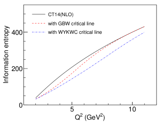
Figure 3: The evolution of information entropy of gluon distribution in $x$ range [$10^{-7}$, $10^{-6}$], from CT14 PDF (solid curve) Dulat et al. (2016), the ideal saturation with GBW critical line (dashed curve) Golec-Biernat and Wusthoff (1998); Bartels et al. (2002); Kowalski and Teaney (2003), and the ideal saturation with WYKWC critical line (dash-dotted curve) Wang et al. (2021).

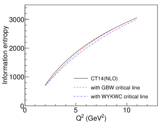
Figure 4: The evolution of information entropy of gluon distribution in the whole $x$ range [$10^{-7}$, $1$], from CT14 PDF (solid curve) Dulat et al. (2016), the ideal saturation with GBW critical line (dashed curve) Golec-Biernat and Wusthoff (1998); Bartels et al. (2002); Kowalski and Teaney (2003), and the ideal saturation with WYKWC critical line (dash-dotted curve) Wang et al. (2021).

There are some great progresses on the entanglement entropy of partons recently. The entanglement entropy at small $x$ is suggested to be $S(x)={\rm ln}[xg(x)]$, and the DIS probes a maximally entangled state Kharzeev and Levin (2017); Tu et al. (2020). The entanglement entropy is also studied with the CGC-Black Hole correspondence Kou et al. (2022). The time evolution of the produced entanglement entropy can be described with Lipatov’s spin chain model Zhang et al. (2022). Within this model, the gluon structure function should grow as $xg(x)\sim 1/x^{1/3}$. The defined classical information entropy in this work is different from the quantum entanglement entropy of the partons at a given $x$ and $Q^{2}$ discussed in Refs. Kharzeev and Levin (2017); Tu et al. (2020). In this paper, the Bjorken $x$ is not fixed and treated as a random variable. The classical entropy in this work quantifies specifically the “choice” of the random variable $x$ in the measurements, while the quantum entanglement entropy quantifies the “choice” of the parton density or the hadron multiplicity at a fixed $x$. Moreover, the quantum entanglement entropy is the quantum information entropy, which quantifies the degree of mixing of the mixed state of a given finite system, or the “departure” of the subsystem from a pure state. Different entropies characterize the different complexities of the system in different aspects. Therefore there is no contradiction between the classical information entropy in this work and the recently proposed entanglement entropy.

There is also the semiclassical Wehrl entropy of parton distributions defined with the Wigner distribution and Husimi distribution Hagiwara et al. (2018). The classical entropy in this work is different from the semiclassical entropy mainly in the following two aspects. (1) The entropy in Ref. Hagiwara et al. (2018) quantifies the complexity of the multi-parton distributions in transverse phase space $(b_{\perp},k_{\perp})$ with $x$ fixed, while this paper focuses on the entropy of the probability distribution of $x$. These two entropies should be applied for different measurements of different variables. (2) The entropy in Ref. Hagiwara et al. (2018) is the semiclassical entropy based on the QCD Husimi distribution, while the entropy defined in this work is a classical information entropy based on probability density distribution.

In summary, many classical and quantum entropies of the hadronic system are defined, and they are the basic and new ways to characterize the complicated hadron structure. Different entropies quantify the complexities of the hadron structure from different angles, such as the hadron multiplicity of parton “liberation”, the transverse momentum distribution, and the longitudinal momentum distribution. Therefore different entropies are applied to different physical questions. For the newly defined information entropy of PDFs, it can be applied in distinguishing the gluon saturation in experiment. Although determining PDFs from experimental measurements is a quite traditional way of probing the nucleon structure, simply obtaining the gluon distribution is still quite helpful in tackling the saturation phenomenon at small $x$. Therefore the conventional processes which are sensitive to the gluon distribution should also be considered for the exploration of gluon saturation, such as direct photon production Kumar et al. (2003); Campbell et al. (2018); Boettcher (2019), heavy quarkonium production Acharya et al. (2017); Rezaeian and Schmidt (2013); Toll and Ullrich (2013), open charm hadron production Kelsey et al. (2021), and jet production Stump et al. (2003); Pumplin et al. (2009) at current hadron colliders and the future Electron-Ion Collider Abdul Khalek et al. (2022); Accardi et al. (2016). With the concept of entropy, especially the linear evolution of the entropy over the $Q^{2}$ scale, the signal of gluon saturation can be clearly identified. In order to probe the gluon saturation at relatively higher $Q^{2}$ and larger $x$, the heavy nuclear target should be used, as the strong nuclear shadowing and gluon fusion enlarge the domain of gluon saturation.

appendix:

A simple proof of the super-additive property of the classical information entropy in Eq. (1) is provided here. $N_{f}$, $N_{g}$ and $k$ are taken to denote respectively the definite integrals of the density distributions and the ratio between them, as,

$$\begin{split}N_{f}\equiv\int f(x)dx,\\ N_{g}\equiv\int g(x)dx,\\ k\equiv N_{g}/N_{f}.\end{split}$$ (9)

Rewriting the formula of the supper-additive property, we simply need to prove the inequality: $S[f(x)+g(x)]-S[f(x)]-S[g(x)]\geq 0$. According to the definition, one has,

$$\begin{split}S[f(x)+g(x)]-S[f(x)]-S[g(x)]=\\ -\int(f(x)+g(x)){\rm ln}(f(x)+g(x))dx\\ +(N_{f}+N_{g}){\rm ln}(N_{f}+N_{g})\\ +\int f(x){\rm ln}(f(x))dx-N_{f}{\rm ln}(N_{f})\\ +\int g(x){\rm ln}(g(x))dx-N_{g}{\rm ln}(N_{g})\\ =N_{f}{\rm ln}\left(\frac{N_{f}+N_{g}}{N_{f}}\right)+\int f(x){\rm ln}\left(\frac{f(x)}{f(x)+g(x)}\right)dx\\ +N_{g}{\rm ln}\left(\frac{N_{f}+N_{g}}{N_{g}}\right)+\int g(x){\rm ln}\left(\frac{g(x)}{f(x)+g(x)}\right)dx\\ =\int f(x){\rm ln}\left(\frac{N_{f}+N_{g}}{N_{f}}\frac{f(x)}{f(x)+g(x)}\right)dx\\ +\int g(x){\rm ln}\left(\frac{N_{f}+N_{g}}{N_{g}}\frac{g(x)}{f(x)+g(x)}\right)dx.\\ \end{split}$$ (10)

For any given $g(x)$, one can construct a function $\delta(x)$ as,

$$\begin{split}\delta(x)\equiv g(x)-kf(x),\\ g(x)\equiv kf(x)+\delta(x),\end{split}$$ (11)

in which the $k$ is defined in Eq. (9). From a simple calculation, one finds that $\int\delta(x)dx=0$. The function $\delta(x)$ can be viewed as an oscillating function of $x$ which describes the variations of $g(x)$ from $kf(x)$. With the constructed $\delta(x)$ function and the definition of $k$, one has,

$$\begin{split}\int f(x){\rm ln}\left(\frac{N_{f}+N_{g}}{N_{f}}\frac{f(x)}{f(x)+g(x)}\right)dx\\ =\int f(x){\rm ln}\left(\frac{(1+k)N_{f}}{N_{f}}\frac{f(x)}{(1+k)f(x)+\delta(x)}\right)dx.\end{split}$$ (12)

The Taylor expansion of $f(x)/[(1+k)f(x)+\delta(x)]$ in terms of $\delta(x)$ is written as,

$$\begin{split}\frac{f(x)}{(1+k)f(x)+\delta(x)}=\frac{f(x)}{(1+k)f(x)}-\frac{f(x)\delta(x)}{[(1+k)f(x)]^{2}}+\cdot\cdot\cdot\\ =\frac{1}{(1+k)}-\frac{\delta(x)}{(1+k)^{2}f(x)}+\cdot\cdot\cdot\end{split}$$ (13)

By taking the two leading terms of the Taylor expansion, Eq. (12) is simplified as,

$$\begin{split}\int f(x){\rm ln}\left(\frac{N_{f}+N_{g}}{N_{f}}\frac{f(x)}{f(x)+g(x)}\right)dx\\ =\int f(x){\rm ln}\left(\frac{(1+k)N_{f}}{N_{f}}\frac{f(x)}{(1+k)f(x)+\delta(x)}\right)dx\\ =\int f(x){\rm ln}\left(1-\frac{\delta(x)}{(1+k)f(x)}\right)dx.\end{split}$$ (14)

Let us look at the Taylor expansion of ${\rm ln}\left(1-\frac{\delta(x)}{(1+k)f(x)}\right)$, which is written as,

$$\begin{split}{\rm ln}\left(1-\frac{\delta(x)}{(1+k)f(x)}\right)=\\ {\rm ln}(1)-\frac{\delta(x)}{(1+k)f(x)}+\frac{1}{2}\frac{\delta^{2}(x)}{(1+k)^{2}f^{2}(x)}+\cdot\cdot\cdot\\ =-\frac{\delta(x)}{(1+k)f(x)}+\frac{1}{2}\frac{\delta^{2}(x)}{(1+k)^{2}f^{2}(x)}+\cdot\cdot\cdot\end{split}$$ (15)

By taking the leading terms of the expansion, one has,

$$\begin{split}\int f(x){\rm ln}\left(1-\frac{\delta(x)}{(1+k)f(x)}\right)dx=\\ \int f(x)\left[-\frac{\delta(x)}{(1+k)f(x)}+\frac{1}{2}\frac{\delta^{2}(x)}{(1+k)^{2}f^{2}(x)}\right]dx\\ =-\frac{1}{1+k}\int\delta(x)dx+\frac{1}{2(1+k)^{2}}\int\frac{\delta^{2}(x)}{f(x)}dx.\end{split}$$ (16)

Since $\int\delta(x)dx=0$ is provided by definition and $\delta^{2}(x)/f(x)$ is always non-negative, one has,

$$\begin{split}\int f(x){\rm ln}\left(\frac{N_{f}+N_{g}}{N_{f}}\frac{f(x)}{f(x)+g(x)}\right)dx\\ =\int f(x){\rm ln}\left(1-\frac{\delta(x)}{(1+k)f(x)}\right)dx\\ =-\frac{1}{1+k}\int\delta(x)dx+\frac{1}{2(1+k)^{2}}\int\frac{\delta^{2}(x)}{f(x)}dx\\ \geq 0.\end{split}$$ (17)

Similarly, one also has,

$$\begin{split}\int g(x){\rm ln}\left(\frac{N_{f}+N_{g}}{N_{g}}\frac{g(x)}{f(x)+g(x)}\right)dx\\ =\int g(x){\rm ln}\left(\frac{N_{f}+N_{g}}{N_{g}}\left(1-\frac{f(x)}{f(x)+g(x)}\right)\right)dx\\ =\int g(x){\rm ln}\left(1+\frac{\delta(x)}{k(1+k)f(x)}\right)dx.\end{split}$$ (18)

By taking the leading term of the Taylor expansion of ${\rm ln}\left(1+\frac{\delta(x)}{k(1+k)f(x)}\right)$, one has,

$$\begin{split}\int g(x){\rm ln}\left(\frac{N_{f}+N_{g}}{N_{g}}\frac{g(x)}{f(x)+g(x)}\right)dx\\ =\int g(x){\rm ln}\left(1+\frac{\delta(x)}{k(1+k)f(x)}\right)dx\\ =\frac{1}{k(1+k)}\int\frac{g(x)\delta(x)}{f(x)}dx\\ =\frac{1}{k(1+k)}\int\left(k\delta(x)+\frac{\delta^{2}(x)}{f(x)}\right)dx\\ =\frac{1}{k(1+k)}\int\frac{\delta^{2}(x)}{f(x)}dx\geq 0.\end{split}$$ (19)

Now I have proved that,

$$\begin{split}\int f(x){\rm ln}\left(\frac{N_{f}+N_{g}}{N_{f}}\frac{f(x)}{f(x)+g(x)}\right)dx\geq 0,\end{split}$$ (20)

and

$$\begin{split}\int g(x){\rm ln}\left(\frac{N_{f}+N_{g}}{N_{g}}\frac{g(x)}{f(x)+g(x)}\right)dx\geq 0.\end{split}$$ (21)

Therefore, the inequality is finally proved, as,

$$\begin{split}S[f(x)+g(x)]-S[f(x)]-S[g(x)]=\\ =\int f(x){\rm ln}\left(\frac{N_{f}+N_{g}}{N_{f}}\frac{f(x)}{f(x)+g(x)}\right)dx\\ +\int g(x){\rm ln}\left(\frac{N_{f}+N_{g}}{N_{g}}\frac{g(x)}{f(x)+g(x)}\right)dx\\ \geq 0.\end{split}$$ (22)

Note that in the deduction, the function $\delta(x)$ is required to be a small variation, i.e., $\delta(x)$ is required to be much lower than $f(x)$. Based on the definition in Eq. (9), the requirement is met as long as both $g(x)$ and $k$ are small. In principle, $g(x)$ can be divided into a lot of functions which are close to zero, as $g(x)=\sum_{i=1}^{i=n}g(x)/n$ with $(g(x)/n)/f(x)<\epsilon$. Therefore, the supper-additive property of the classical information entropy is proved, as,

$$\begin{split}S[f(x)+g(x)]=S\left[f(x)+\sum_{i=1}^{i=n}g(x)/n\right]\\ \geq S\left[f(x)+\sum_{i=1}^{i=n-1}g(x)/n\right]+S[g(x)/n]\\ \geq S\left[f(x)+\sum_{i=1}^{i=n-2}g(x)/n\right]+2S[g(x)/n]\\ \cdot\cdot\cdot\\ \geq S[f(x)]+nS[g(x)/n]=S[f(x)]+S[g(x)].\end{split}$$ (23)

References

- Bjorken (1969) J. D. Bjorken, Phys. Rev. 179, 1547 (1969).
- Feynman (1969) R. P. Feynman, Phys. Rev. Lett. 23, 1415 (1969).
- Bjorken and Paschos (1969) J. D. Bjorken and E. A. Paschos, Phys. Rev. 185, 1975 (1969).
- Gribov (1973) V. N. Gribov, (1973), arXiv:hep-ph/0006158 .
- Collins and Soper (1987) J. C. Collins and D. E. Soper, Ann. Rev. Nucl. Part. Sci. 37, 383 (1987).
- Collins et al. (1989) J. C. Collins, D. E. Soper, and G. F. Sterman, Adv. Ser. Direct. High Energy Phys. 5, 1 (1989), arXiv:hep-ph/0409313 .
- Sterman (1995) G. F. Sterman, in Theoretical Advanced Study Institute in Elementary Particle Physics (TASI 95): QCD and Beyond (1995) pp. 327–408, arXiv:hep-ph/9606312 .
- Yang and Mills (1954) C.-N. Yang and R. L. Mills, Phys. Rev. 96, 191 (1954).
- Gross and Wilczek (1973) D. J. Gross and F. Wilczek, Phys. Rev. Lett. 30, 1343 (1973).
- Politzer (1973) H. D. Politzer, Phys. Rev. Lett. 30, 1346 (1973).
- Dulat et al. (2016) S. Dulat, T.-J. Hou, J. Gao, M. Guzzi, J. Huston, P. Nadolsky, J. Pumplin, C. Schmidt, D. Stump, and C. P. Yuan, Phys. Rev. D 93, 033006 (2016), arXiv:1506.07443 [hep-ph] .
- Ball et al. (2010) R. D. Ball, L. Del Debbio, S. Forte, A. Guffanti, J. I. Latorre, J. Rojo, and M. Ubiali, Nucl. Phys. B 838, 136 (2010), arXiv:1002.4407 [hep-ph] .
- Ball et al. (2012) R. D. Ball, V. Bertone, F. Cerutti, L. Del Debbio, S. Forte, A. Guffanti, J. I. Latorre, J. Rojo, and M. Ubiali (NNPDF), Nucl. Phys. B 855, 153 (2012), arXiv:1107.2652 [hep-ph] .
- Shannon (1948) C. E. Shannon, The Bell System Technical Journal 27, 379 (1948).
- Jaynes (1957a) E. T. Jaynes, Phys. Rev. 106, 620 (1957a).
- Jaynes (1957b) E. T. Jaynes, Phys. Rev. 108, 171 (1957b).
- Wang and Chen (2015) R. Wang and X. Chen, Phys. Rev. D 91, 054026 (2015), arXiv:1410.3598 [hep-ph] .
- Gribov et al. (1983) L. V. Gribov, E. M. Levin, and M. G. Ryskin, Phys. Rept. 100, 1 (1983).
- Mueller and Qiu (1986) A. H. Mueller and J.-w. Qiu, Nucl. Phys. B 268, 427 (1986).
- Mueller (1990) A. H. Mueller, Nucl. Phys. B 335, 115 (1990).
- Mueller (1999) A. H. Mueller, Nucl. Phys. B 558, 285 (1999), arXiv:hep-ph/9904404 .
- McLerran and Venugopalan (1994a) L. D. McLerran and R. Venugopalan, Phys. Rev. D 49, 2233 (1994a), arXiv:hep-ph/9309289 .
- McLerran and Venugopalan (1994b) L. D. McLerran and R. Venugopalan, Phys. Rev. D 49, 3352 (1994b), arXiv:hep-ph/9311205 .
- McLerran and Venugopalan (1994c) L. D. McLerran and R. Venugopalan, Phys. Rev. D 50, 2225 (1994c), arXiv:hep-ph/9402335 .
- Balitsky (1996) I. Balitsky, Nucl. Phys. B 463, 99 (1996), arXiv:hep-ph/9509348 .
- Jalilian-Marian et al. (1997) J. Jalilian-Marian, A. Kovner, A. Leonidov, and H. Weigert, Nucl. Phys. B 504, 415 (1997), arXiv:hep-ph/9701284 .
- Iancu et al. (2001a) E. Iancu, A. Leonidov, and L. D. McLerran, Nucl. Phys. A 692, 583 (2001a), arXiv:hep-ph/0011241 .
- Weigert (2002) H. Weigert, Nucl. Phys. A 703, 823 (2002), arXiv:hep-ph/0004044 .
- Iancu et al. (2001b) E. Iancu, A. Leonidov, and L. D. McLerran, Phys. Lett. B 510, 133 (2001b), arXiv:hep-ph/0102009 .
- Jalilian-Marian and Kovchegov (2006) J. Jalilian-Marian and Y. V. Kovchegov, Prog. Part. Nucl. Phys. 56, 104 (2006), arXiv:hep-ph/0505052 .
- Gelis et al. (2010) F. Gelis, E. Iancu, J. Jalilian-Marian, and R. Venugopalan, Ann. Rev. Nucl. Part. Sci. 60, 463 (2010), arXiv:1002.0333 [hep-ph] .
- Balitsky (1997) I. Balitsky, AIP Conf. Proc. 407, 953 (1997), arXiv:hep-ph/9706411 .
- Kovchegov (1999) Y. V. Kovchegov, Phys. Rev. D 60, 034008 (1999), arXiv:hep-ph/9901281 .
- Kovchegov (2000) Y. V. Kovchegov, Phys. Rev. D 61, 074018 (2000), arXiv:hep-ph/9905214 .
- Balitsky (2001) I. Balitsky, Phys. Lett. B 518, 235 (2001), arXiv:hep-ph/0105334 .
- Lipatov (1976) L. N. Lipatov, Sov. J. Nucl. Phys. 23, 338 (1976).
- Kuraev et al. (1977) E. A. Kuraev, L. N. Lipatov, and V. S. Fadin, Sov. Phys. JETP 45, 199 (1977).
- Balitsky and Lipatov (1978) I. I. Balitsky and L. N. Lipatov, Sov. J. Nucl. Phys. 28, 822 (1978).
- Froissart (1961) M. Froissart, Phys. Rev. 123, 1053 (1961).
- Martin (1963) A. Martin, Phys. Rev. 129, 1432 (1963).
- Morreale and Salazar (2021) A. Morreale and F. Salazar, Universe 7, 312 (2021), arXiv:2108.08254 [hep-ph] .
- Tong et al. (2023) X.-B. Tong, B.-W. Xiao, and Y.-Y. Zhang, Phys. Rev. Lett. 130, 151902 (2023), arXiv:2211.01647 [hep-ph] .
- Golec-Biernat and Wusthoff (1998) K. J. Golec-Biernat and M. Wusthoff, Phys. Rev. D 59, 014017 (1998), arXiv:hep-ph/9807513 .
- Bartels et al. (2002) J. Bartels, K. J. Golec-Biernat, and H. Kowalski, Phys. Rev. D 66, 014001 (2002), arXiv:hep-ph/0203258 .
- Kowalski and Teaney (2003) H. Kowalski and D. Teaney, Phys. Rev. D 68, 114005 (2003), arXiv:hep-ph/0304189 .
- Wang et al. (2021) X. Wang, Y. Yang, W. Kou, R. Wang, and X. Chen, Phys. Rev. D 103, 056008 (2021), arXiv:2009.13325 [hep-ph] .
- Nikolaev and Zakharov (1991) N. N. Nikolaev and B. G. Zakharov, Z. Phys. C 49, 607 (1991).
- Kharzeev and Levin (2017) D. E. Kharzeev and E. M. Levin, Phys. Rev. D 95, 114008 (2017), arXiv:1702.03489 [hep-ph] .
- Tu et al. (2020) Z. Tu, D. E. Kharzeev, and T. Ullrich, Phys. Rev. Lett. 124, 062001 (2020), arXiv:1904.11974 [hep-ph] .
- Kou et al. (2022) W. Kou, X. Wang, and X. Chen, Phys. Rev. D 106, 096027 (2022), arXiv:2208.07521 [hep-ph] .
- Zhang et al. (2022) K. Zhang, K. Hao, D. Kharzeev, and V. Korepin, Phys. Rev. D 105, 014002 (2022), arXiv:2110.04881 [quant-ph] .
- Hagiwara et al. (2018) Y. Hagiwara, Y. Hatta, B.-W. Xiao, and F. Yuan, Phys. Rev. D 97, 094029 (2018), arXiv:1801.00087 [hep-ph] .
- Kumar et al. (2003) A. Kumar, M. Kumar Jha, B. Mitra Sodermark, A. Bhardwaj, K. Ranjan, and R. K. Shivpuri, Phys. Rev. D 67, 014016 (2003).
- Campbell et al. (2018) J. M. Campbell, J. Rojo, E. Slade, and C. Williams, Eur. Phys. J. C 78, 470 (2018), arXiv:1802.03021 [hep-ph] .
- Boettcher (2019) T. Boettcher (LHCb), Nucl. Phys. A 982, 251 (2019).
- Acharya et al. (2017) S. Acharya et al. (ALICE), Eur. Phys. J. C 77, 392 (2017), arXiv:1702.00557 [hep-ex] .
- Rezaeian and Schmidt (2013) A. H. Rezaeian and I. Schmidt, Phys. Rev. D 88, 074016 (2013), arXiv:1307.0825 [hep-ph] .
- Toll and Ullrich (2013) T. Toll and T. Ullrich, Phys. Rev. C 87, 024913 (2013), arXiv:1211.3048 [hep-ph] .
- Kelsey et al. (2021) M. Kelsey, R. Cruz-Torres, X. Dong, Y. Ji, S. Radhakrishnan, and E. Sichtermann, Phys. Rev. D 104, 054002 (2021), arXiv:2107.05632 [hep-ph] .
- Stump et al. (2003) D. Stump, J. Huston, J. Pumplin, W.-K. Tung, H. L. Lai, S. Kuhlmann, and J. F. Owens, JHEP 10, 046 (2003), arXiv:hep-ph/0303013 .
- Pumplin et al. (2009) J. Pumplin, J. Huston, H. L. Lai, P. M. Nadolsky, W.-K. Tung, and C. P. Yuan, Phys. Rev. D 80, 014019 (2009), arXiv:0904.2424 [hep-ph] .
- Abdul Khalek et al. (2022) R. Abdul Khalek et al., Nucl. Phys. A 1026, 122447 (2022), arXiv:2103.05419 [physics.ins-det] .
- Accardi et al. (2016) A. Accardi et al., Eur. Phys. J. A 52, 268 (2016), arXiv:1212.1701 [nucl-ex] .