Accelerating Universe scenario in anisotropic $f\left(Q\right)$ cosmology

Abstract

In this paper, we investigate the exact solution of an anisotropic space-time in the context of $f(Q)$ gravity, where $f\left(Q\right)$ is the arbitrary function of the non-metricity scalar $Q$. Here, we consider a specific power-law form as $f\left(Q\right)=\alpha Q^{n+1}+\beta$, where $\alpha$, $\beta$, and $n$ are free model parameters. Using power-law cosmology ($a\left(t\right)\propto t^{m}$), we analyze the physical behavior of cosmological parameters such as the energy density, pressure, EoS parameter, skewness parameter. Further, we validated the model with energy conditions and found that our $f\left(Q\right)$ cosmological model behaves like the quintessence model in the present and $\Lambda$CDM in the future.

I Introducion

One of the most common problems in modern cosmology is the problem of the current expansion of the Universe. General Relativity (GR) as the theoretical framework of modern cosmology says that the expansion of the Universe is decelerating, but astrophysical observational data have a different opinion: the current Universe is in an acceleration phase [1, 2, 3, 4, 5, 6, 7, 8, 9, 10, 11, 12]. The phenomenon of cosmic inflation and the problem of initial singularity is other subjects of discussion [13, 14]. Before Hubble showed through observations that our universe is expanding, cosmologists believed that our universe is stable and static, so Einstein added a small positive cosmological constant ($\Lambda$) to his field equations to go with this idea, after which Einstein described that the cosmological constant is the biggest mistake in his life. In the late 1990s, it was shown that the cosmological constant was returned because it might be a suitable candidate for Dark Energy (DE). DE is a strange form of energy that has negative pressure $(p)$ and positive energy density $(\rho)$ and is assumed to be responsible for the cosmic acceleration. DE has a negative equation of state (EoS) parameter $(\omega=\frac{p}{\rho}<0)$, and we can classify other DE models by this parameter, i.e. quintessence $-1<\omega<-0.33$, cosmological constant $\omega=-1$, phantom DE $\omega<-1$ [15, 16, 17, 18].

Another proposal to explain the current acceleration of the Universe comes from modified theories of gravity (MTG) [19] . One of the most recently developed examples is the $f\left(Q\right)$ theory of gravity or the symmetric teleparallel gravity (STG) [20]. This theory is a generalized version of teleparallel gravity [21] in which gravity is caused to the non-metricity and where $f\left(Q\right)$ is an arbitrary function of the non-metricity scalar $Q$. In this theory, the geometry is torsion and curvature free and the non-metricity term $Q$ only determines the gravitational interactions. The STG is demonstrated in the so-called coincidence gauge by assuming that the connection is symmetric [22]. The geometric basis of GR is Riemannian geometry, while gravity $f\left(Q\right)$ whose basis is Weyl geometry which is a generalization of Riemannian geometry [23, 24]. Also Weyl geometry is a particular case of Weyl-Cartan geometry in which torsion disappears [25]. The interesting about this theory is that it could explain the current acceleration of the Universe like other MTG without using DE [26]. Many works have been done in this context so far. The first cosmological solutions in $f\left(Q\right)$ gravity are discussed in [27]. Mandal et al. presented a complete analysis of energy conditions for $f\left(Q\right)$ gravity models and constraint families of $f\left(Q\right)$ models compatible with the present accelerating expansion of the Universe [28]. In addition, the cosmography in $f\left(Q\right)$ gravity is considered by Mandal et al. [29]. The growth index of matter perturbations has been examined in the context of $f\left(Q\right)$ gravity in [30] and, several other issues in $f\left(Q\right)$ gravity are discussed in [31, 32, 33].

According to the cosmological principle, isotropic models of the Universe are most suitable for studying the structure of the Universe on a large scale. Nevertheless, cosmologists believe that the early universe may not have been completely uniform. Further, the theoretical arguments and the anomalies observed in the CMB (Cosmic Microwave Background) are clear evidence of the existence of an anisotropic phase, which was later called the isotropic phase [34, 35]. This forecasting motivates us to create cosmological models in the early phases of the Universe with models that have an anisotropic background. Hence, the presence of anisotropy in the early phases of the Universe is an intriguing topic to study. There are models in cosmology that respect these criteria called Bianchi models, a Bianchi type-I is one such anisotropic cosmological model that is considered a generalization of the flat Friedmann-Lemaître-Robertson-Walker (FLRW) model. Therefore, in this work, we will explore Bianchi type-I models in the context of $f(Q)$ gravity because it is an interesting and still very new topic. Exact solutions of the symmetric teleparallel gravity field equations for a locally rotationally symmetric (LRS) Bianchi type-I space-time were studied in [36]. Solutions of a Bianchi type-I space-time were examined in [37] using the hybrid expansion law.

This manuscript is organized as follows: In Sec II, we presented a brief description of the mathematical formalism of $f(Q)$ gravity. In Sec. III, the field equations in anisotropic space-time are evaluated for $f\left(Q\right)$ gravity. In Sec. IV, we have discussed the energy conditions in $f(Q)$ gravity. In Sec. V, we consider the specific power-law form of $f(Q)$ gravity as $f\left(Q\right)=\alpha Q^{n+1}+\beta$, where $\alpha$, $\beta$, and $n$ are free model parameters. Further, we discussed the behavior of several cosmological parameters in the same section. Lastly, we discussed our conclusions in Sec. VI.

II Brief description of the mathematical formalism of $f(Q)$ gravity

In Weyl-Cartan geometry, the so-called symmetric metric tensor $g_{\mu\nu}$ can be considered as a generalization of the gravitational potential, and it is fundamentally used to define the length of a vector, and we also need an asymmetric connection $\Sigma{{}^{\gamma}}_{\mu\nu}$ to defines the covariant derivatives and parallel transport. Thus, the general affine connection can be decomposed into three elements: the Christoffel symbol ${\Gamma^{\gamma}}_{\mu\nu}$, the contortion tensor ${C^{\gamma}}_{\mu\nu}$, and the disformation tensor ${L^{\gamma}}_{\mu\nu}$, respectively, which is given by [22]

$$\Sigma{{}^{\gamma}}_{\mu\nu}={\Gamma^{\gamma}}_{\mu\nu}+{C^{\gamma}}_{\mu\nu}+{L^{\gamma}}_{\mu\nu},$$ (1)

where the Levi-Civita connection ${\Gamma^{\gamma}}_{\mu\nu}$ of the metric $g_{\mu\nu}$ has the form

$${\Gamma^{\gamma}}_{\mu\nu}\equiv\frac{1}{2}g^{\gamma\sigma}\left(\frac{\partial g_{\sigma\nu}}{\partial x^{\mu}}+\frac{\partial g_{\sigma\mu}}{\partial x^{\nu}}-\frac{\partial g_{\mu\nu}}{\partial x^{\sigma}}\right),$$ (2)

the contorsion tensor ${C^{\gamma}}_{\mu\nu}$ can be written as

$${C^{\gamma}}_{\mu\nu}\equiv\frac{1}{2}{T^{\gamma}}_{\mu\nu}+T_{(\mu}{}^{\gamma}{}_{\nu)},$$ (3)

where ${T^{\gamma}}_{\mu\nu}\equiv 2{\Sigma^{\gamma}}_{[\mu\nu]}$ in Eq. (3) is the torsion tensor. Finally, the disformation tensor ${L^{\gamma}}_{\mu\nu}$ is derived from the non-metricity tensor $Q_{\gamma\mu\nu}$ as

$${L^{\gamma}}_{\mu\nu}\equiv\frac{1}{2}g^{\gamma\sigma}\left(Q_{\nu\mu\sigma}+Q_{\mu\nu\sigma}-Q_{\gamma\mu\nu}\right).$$ (4)

In the above equation, the non-metricity tensor $Q_{\gamma\mu\nu}$ is specific as the (minus) covariant derivative of the metric tensor with regard to the Weyl-Cartan connection $\Sigma{{}^{\gamma}}_{\mu\nu}$, i.e. $Q_{\gamma\mu\nu}=\nabla_{\gamma}g_{\mu\nu}$, and it can be obtained

$$Q_{\gamma\mu\nu}=-\frac{\partial g_{\mu\nu}}{\partial x^{\gamma}}+g_{\nu\sigma}\Sigma{{}^{\sigma}}_{\mu\gamma}+g_{\sigma\mu}\Sigma{{}^{\sigma}}_{\nu\gamma}.$$ (5)

The connection is presumed to be torsionless and curvatureless within the current background. It corresponds to the pure coordinate transformation from the trivial connection mentioned in [20]. Thus, for a flat and torsion-free connection, the connection (1) can be parameterized as

$$\Sigma{{}^{\gamma}}_{\mu\beta}=\frac{\partial x^{\gamma}}{\partial\xi^{\rho}}\partial_{\mu}\partial_{\beta}\xi^{\rho}.$$ (6)

Now, $\xi^{\gamma}=$ $\xi^{\gamma}\left(x^{\mu}\right)$ is an invertible relation. It is always possible to get a coordinate system so that the connection $\Sigma{{}^{\gamma}}_{\mu\nu}$ vanish. This condition is called coincident gauge and has been used in many studies of symmetric teleparallel equivalent to GR (STEGR) and in this condition the covariant derivative $\nabla_{\gamma}$ reduces to the partial derivative $\partial_{\gamma}$ [22]. Thus, in the coincident gauge coordinate, we get

$$Q_{\gamma\mu\nu}=-\partial_{\gamma}g_{\mu\nu}.$$ (7)

The STG is a geometric description of gravity equivalent to GR within coincident gauge coordinates in which $\Sigma_{\mu\nu}=0$ and ${C^{\gamma}}_{\mu\nu}=0$, and consequently from Eq. (1) we can conclude that [22]

$${\Gamma^{\gamma}}_{\mu\nu}=-{L^{\gamma}}_{\mu\nu}.$$ (8)

The $f\left(Q\right)$ theory of gravity is a generalization or modification of the symmetric teleparallel equivalent of GR. The action for this theory is given [20, 27, 28, 29]

$$S=\int\left[\frac{1}{2\kappa}f(Q)+\mathcal{L}_{m}\right]d^{4}x\sqrt{-g},$$ (9)

where $\kappa=8\pi G=1$, $f(Q)$ can be expressed as the arbitrary function of non-metricity scalar $Q$, $g$ is the determinant of the metric tensor $g_{\mu\nu}$, and $\mathcal{L}_{m}$ is the matter Lagrangian density. Now, the non-metricity tensor $Q_{\gamma\mu\nu}$ and its traces can be written as

$$Q_{\gamma\mu\nu}=\nabla_{\gamma}g_{\mu\nu}\,,$$ (10)

$$Q_{\gamma}={{Q_{\gamma}}^{\mu}}_{\mu}\,,\qquad\widetilde{Q}_{\gamma}={Q^{\mu}}_{\gamma\mu}\,.$$ (11)

In addition, the superpotential tensor (non-metricity conjugate) can be expressed as

$$4{P^{\gamma}}_{\mu\nu}=-{Q^{\gamma}}_{\mu\nu}+2Q_{({\mu^{{}^{\gamma}}}{\nu})}-Q^{\gamma}g_{\mu\nu}-\widetilde{Q}^{\gamma}g_{\mu\nu}-\delta_{{(\gamma^{{}^{Q}}}\nu)}^{\gamma}\,,$$ (12)

where the trace of the non-metricity tensor can be obtained as

$$Q=-Q_{\gamma\mu\nu}P^{\gamma\mu\nu}\,.$$ (13)

Now, the matter energy-momentum tensor is defined as

$$T_{\mu\nu}=-\frac{2}{\sqrt{-g}}\frac{\delta(\sqrt{-g}\mathcal{L}_{m})}{\delta g^{\mu\nu}}\,.$$ (14)

By varying the modified Einstein-Hilbert action (9) with respect to the metric tensor $g_{\mu\nu}$, the gravitational field equations obtained as

$$\frac{2}{\sqrt{-g}}\nabla_{\gamma}\left(\sqrt{-g}f_{Q}P^{\gamma}{}_{\mu\nu}\right)-\frac{1}{2}fg_{\mu\nu}+f_{Q}\left(P_{\mu\gamma i}Q_{\nu}{}^{\gamma i}-2Q_{\gamma i\mu}P^{\gamma i}{}_{\nu}\right)=T_{\mu\nu},$$ (15)

where $f_{Q}=\frac{df}{dQ}$ and $\nabla_{\gamma}$ denotes the covariant derivative.

III $f\left(Q\right)$ field equations in anisotropic space-time

The standard FLRW Universe is isotropic and homogeneous. Hence, to address the anisotropic nature of the Universe in $f\left(Q\right)$ gravity, which manifests as anomalies found in the CMB, the Bianchi type-I Universe is indeed important because it represents a spatially homogeneous, but not isotropic. Thus, we consider a Bianchi-type I space-time in the form

$$ds^{2}=-dt^{2}+A^{2}(t)dx^{2}+B^{2}(t)(dy^{2}+dz^{2}),$$ (16)

where metric potentials $A\left(t\right)$ and $B\left(t\right)$ depend only on cosmic time $\left(t\right)$. Here, to complete the choice of the anisotropic type space-time, the equation of state (EoS) parameter of the gravitational fluid must also be generalized, and from another point of view, to give a more reasonable model, an anisotropic nature must be exhibited as described in [38]. Thus, the energy-momentum tensor for the anisotropic fluid can be expressed as

$$T_{\nu}^{\mu} =\text{diag}(-\rho,p_{x},p_{y},p_{z})\,,$$ (17)

$$=\text{diag}(-1,\omega_{x},\omega_{y},\omega_{z})\rho,$$

$$=\text{diag}(-1,\omega,(\omega+\delta),(\omega+\delta))\rho,$$

where $\rho$ is the energy density of the anisotropic fluid, $p_{x}$, $p_{y}$, $p_{z}$ are the pressures and $\omega_{x}$, $\omega_{y}$, $\omega_{z}$ are the directional EoS parameters along $x$, $y$ and $z$ coordinates respectively. The deviation from isotropy is parametrized by setting $\omega_{x}=\omega$ and then introducing the deviations along $y$ and $z$ axes by the skewness parameter $\delta$, where $\omega$ and $\delta$ are functions of cosmic time only [36].

For anisotropic fluid as matter contents, the corresponding field equations of Bianchi type-I space-time are obtained as [36]

$$\frac{f}{2}+f_{Q}\left[4\frac{\dot{A}}{A}\frac{\dot{B}}{B}+2\left(\frac{\dot{B}}{B}\right)^{2}\right]=\rho,$$ (18)

$$\frac{f}{2}-f_{Q}\left[-2\frac{\dot{A}}{A}\frac{\dot{B}}{B}-2\frac{\ddot{B}}{B}-2\left(\frac{\dot{B}}{B}\right)^{2}\right]+2\frac{\dot{B}}{B}\dot{Q}f_{QQ}=-\omega\rho,$$ (19)

$$\frac{f}{2}-f_{Q}\left[-3\frac{\dot{A}}{A}\frac{\dot{B}}{B}-\frac{\ddot{A}}{A}-\frac{\ddot{B}}{B}-\left(\frac{\dot{B}}{B}\right)^{2}\right]+\left(\frac{\dot{A}}{A}+\frac{\dot{B}}{B}\right)\dot{Q}f_{QQ}=-(\omega+\delta)\rho,$$ (20)

where the dot $\left(\text{\textperiodcentered}\right)$ denotes the ordinary differentiation with regard to cosmic time $\left(t\right)$. The corresponding non-metricity scalar can be written as

$$Q=-2\left(\frac{\overset{.}{B}}{B}\right)^{2}-4\frac{\overset{.}{A}}{A}\frac{\overset{.}{B}}{B}.$$ (21)

In order to simplify the form of the field equations (18)-(20) and write them in terms of the non-metricity scalar $Q$, the directional Hubble parameters $H_{x}=\frac{\overset{.}{A}}{A},H_{y}=\frac{\overset{.}{B}}{B}$ and average Hubble parameter $H=\frac{1}{3}\left(H_{x}+2H_{y}\right)$, we use the following relations: $\frac{\partial}{\partial t}\left(\frac{\dot{A}}{A}\right)=\frac{\ddot{A}}{A}-\left(\frac{\dot{A}}{A}\right)^{2}$ and $Q=-2H_{y}^{2}-4H_{x}H_{y}$. The field equations (18)-(20) becomes

$$\frac{f}{2}-Qf_{Q}=\rho,$$ (22)

$$\frac{f}{2}+2\frac{\partial}{\partial t}\left[H_{y}f_{Q}\right]+6Hf_{Q}H_{y}=-\omega\rho,$$ (23)

$$\frac{f}{2}+\frac{\partial}{\partial t}\left[f_{Q}(H_{x}+H_{y})\right]+3Hf_{Q}\left(H_{x}+H_{y}\right)=-(\omega+\delta)\rho.$$ (24)

Using Eqs. (22) and (23), the EoS parameter ($\omega=\frac{p}{\rho}$) is

$$\omega=\frac{-1}{\frac{f}{2}-Qf_{Q}}\left[\frac{f}{2}+2\frac{\partial}{\partial t}\left[H_{y}f_{Q}\right]+6Hf_{Q}H_{y}\right].$$ (25)

Similarly, using Eqs. (22), (23) and (24) we find the skewness parameters as

$$\delta=\frac{1}{\frac{f}{2}-Qf_{Q}}\left[\frac{\partial}{\partial t}\left[f_{Q}\left(H_{y}-H_{x}\right)\right]+3Hf_{Q}\left(H_{y}-H_{x}\right)\right].$$ (26)

The above parameters are useful enough to check the validity of the constructed cosmological model, and the reason for expressing them in terms of average Hubble parameter and directional Hubble parameters is that understanding the behavior of the Universe will be more convenient. This means that the volumetric expansion law will remain in a proper form. In [36] the study of anisotropic cosmological models in $f(Q)$ gravity has shown that the solutions can follow the power law using the anisotropy relation ($\theta^{2}\propto\sigma^{2}$). Motivated by this work, we will study here the volumetric power law expansion of the form $V=AB^{2}=t^{m}$, where $m$ be the arbitrary constant that is chosen according to the observational constraints. In the following sections, we will analyze our cosmological models with these considerations.

IV Energy conditions

The energy conditions (ECs) are a set of conditions that describe the geodesics of the Universe. In this background, the ECs are intended to verify the existence of a phase of accelerating expansion of the Universe. Like these condition can be obtained from the well-known Raychaudhury equations, whose forms are [39, 40, 41, 42]

$$\frac{d\theta}{d\tau}=-\frac{1}{3}\theta^{2}-\sigma_{\mu\nu}\sigma^{\mu\nu}+\omega_{\mu\nu}\omega^{\mu\nu}-R_{\mu\nu}u^{\mu}u^{\nu},$$ (27)

$$\frac{d\theta}{d\tau}=-\frac{1}{2}\theta^{2}-\sigma_{\mu\nu}\sigma^{\mu\nu}+\omega_{\mu\nu}\omega^{\mu\nu}-R_{\mu\nu}n^{\mu}n^{\nu}.$$ (28)

Here, $\theta$ is the expansion factor, $n^{\mu}$ is the null vector, and $\sigma^{\mu\nu}$ and $\omega_{\mu\nu}$ are, respectively, the shear and the rotation connected with the vector field $u^{\mu}$. For mathematical details of deriving the Raychaudhury equations in Weyl geometry with the existence of non-metricity, see these references [28, 43]. For attractive gravity, Eqs. (27) and (28) fulfill the following conditions

$$R_{\mu\nu}u^{\mu}u^{\nu}\geq 0,$$ (29)

$$R_{\mu\nu}n^{\mu}n^{\nu}\geq 0.$$ (30)

Hence, if we consider the Universe has a perfect fluid matter distribution, the ECs for $f\left(Q\right)$ gravity are given by

• Weak energy conditions (WEC) if $\rho\geq 0,\rho+p\geq 0$;

• Null energy condition (NEC) if $\rho+\rho\geq 0$;

• Dominant energy conditions (DEC) if $\rho\geq 0,\left|p\right|\leq\rho$.

• Strong energy conditions (SEC) if $\rho+3p\geq 0$.

V Cosmological $f\left(Q\right)$ model

To study the anisotropic nature of the Universe, we consider the specific power law form of $f(Q)$ i.e.

$$f\left(Q\right)=\alpha Q^{n+1}+\beta,$$ (31)

where $\alpha$, $\beta$, and $n$ are free model parameters. This specific functional form for $f(Q)$ was motivated by the work in [26]. For $n=0$ we find the simplest linear form of $f(Q)$ function i.e. $f\left(Q\right)=\alpha Q+\beta$ and for $n=1$ the model takes the non-linear form i.e. $f\left(Q\right)=\alpha Q^{2}+\beta$. In addition, to reduce the number of unknowns, we presumed an anisotropic relation between the directional scale factors in the form $A=B^{k}$ where $k\left(\neq 0,1\right)$ is an arbitrary real number. For a power-law background, the directional scale factors can be derived as: $A\left(t\right)=t^{\frac{km}{k+2}}$, $B\left(t\right)=t^{\frac{m}{k+2}}$. As a result, the directional Hubble parameters are given as: $H_{x}=\left(\frac{km}{k+2}\right)\frac{1}{t}$, $H_{y}=\left(\frac{m}{k+2}\right)\frac{1}{t}$. The above anisotropy relation is chosen on the basis of astronomical observations associated with the velocity redshift relation for extragalactic sources which indicate that the Hubble expansion of the Universe may attain isotropy when $\frac{\sigma}{\theta}$ is constant [44, 45, 46, 47, 48].

Now, using Eq. (31) we find the following expressions for energy density, pressure, EoS parameter, and skewness parameter, respectively.

$$\rho=\frac{1}{2}\left(\beta+\alpha 2^{n+1}\psi^{n+1}-\alpha 2^{n+2}(n+1)\psi^{n+1}\right)$$ (32)

$$p=-\frac{-\alpha(k+2)m2^{n+2}\left(2n^{2}+3n+1\right)\psi^{n}+\alpha m^{2}2^{n+1}(2(k+2)n+3)\psi^{n}+\beta(k+2)^{2}t^{2}}{2(k+2)^{2}t^{2}}$$ (33)

$$\omega=\frac{\alpha(k+2)m2^{n+2}\left(2n^{2}+3n+1\right)\psi^{n}+\alpha m^{2}\left(-2^{n+1}\right)(2(k+2)n+3)\psi^{n}-\beta(k+2)^{2}t^{2}}{\alpha(2k+1)m^{2}2^{n+1}(2n+1)\psi^{n}+\beta(k+2)^{2}t^{2}}$$ (34)

$$\delta=\frac{\alpha(k-1)(k+2)m2^{n+1}(n+1)(-m+2n+1)\psi^{n}}{\alpha(2k+1)m^{2}2^{n+1}(2n+1)\psi^{n}+\beta(k+2)^{2}t^{2}}$$ (35)

where $\psi\left(t\right)=-\frac{(2k+1)m^{2}}{(k+2)^{2}t^{2}}$.

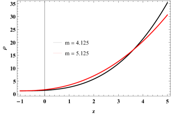
Figure 1: Plot of cosmic energy density ($\rho$) versus redshift ($z$) for $\alpha=-0.001$, $\beta=2.5$, $n=1$ and $k=0.64$.

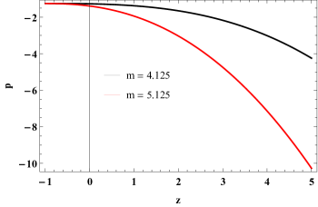
Figure 2: Plot of cosmic pressure ($p$) versus redshift ($z$) for $\alpha=-0.001$, $\beta=2.5$, $n=1$ and $k=0.64$.

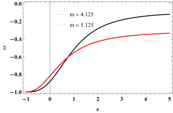
Figure 3: Plot of EoS parameter ($\omega$) versus redshift ($z$) for $\alpha=-0.001$, $\beta=2.5$, $n=1$ and $k=0.64$.

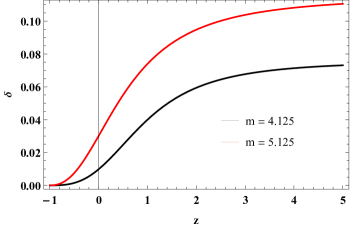
Figure 4: Plot of skewness parameter ($\delta$) versus redshift ($z$) for $\alpha=-0.001$, $\beta=2.5$, $n=1$ and $k=0.64$.

First, all cosmological parameters ($\rho,$ $p,$ $\omega,$ $\delta$) are plotted in terms of cosmic redshift ($z$) with the help of the time-redshift relation $t\left(z\right)=\left(1+z\right)^{-\frac{3}{m}}$ for the different values of $m=4.125$ and $5.125$. From Fig. 1 it is clear that the cosmic energy density remains positive throughout the evolution of the Universe and is an increasing function of cosmic redshift. It starts with a positive value and approaches zero at $z\rightarrow-1$ while Fig. 2 show that the cosmic pressure is a decreasing function of cosmic redshift, which starts with large negative values and tends to zero at $z=0$ (present epoch) and $z\rightarrow-1$ (future). Such behavior of cosmic pressure is caused by the current cosmic acceleration, or so-called DE in the context of GR. Also, from Fig. 3 it can be observed that the EoS parameter is similar to the behavior of quintessence DE at present epoch and converges to the cosmological constant ($\Lambda$) at $z=-1$. Further, Fig. 4 indicates that the skewness parameter starts with a positive value in the past and tends to zero at $z\rightarrow-1$. Hence, the Universe in our model transforms from the phase of anisotropy to the phase of isotropy.

Using Eqs. (32) and (33) in the ECs, we obtain

$$NEC\Leftrightarrow\frac{\alpha m2^{n+1}(n+1)\left(k(m+2n+1)-m+4n+2\right)\psi^{n}}{(k+2)^{2}t^{2}}\geq 0$$ (36)

$$DEC\Leftrightarrow\frac{-\alpha(k+2)m2^{n+1}\left(2n^{2}+3n+1\right)\psi^{n}+\alpha m^{2}2^{n+1}(3kn+k+3n+2)\psi^{n}+\beta(k+2)^{2}t^{2}}{(k+2)^{2}t^{2}}\geq 0$$ (37)

$$SEC\Leftrightarrow-\frac{-3\alpha(k+2)m2^{n+1}\left(2n^{2}+3n+1\right)\psi^{n}+\alpha m^{2}2^{n+1}\left(k(n-1)+5n+4\right)\psi^{n}+\beta(k+2)^{2}t^{2}}{(k+2)^{2}t^{2}}\geq 0$$ (38)

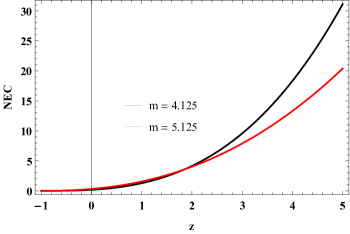
Figure 5: Plot of the NEC versus redshift ($z$) for $\alpha=-0.001$, $\beta=2.5$, $n=1$ and $k=0.64$.

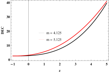
Figure 6: Plot of the DEC versus redshift ($z$) for $\alpha=-0.001$, $\beta=2.5$, $n=1$ and $k=0.64$.

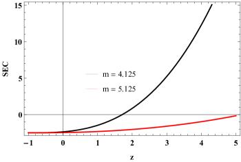
Figure 7: Plot of the SEC versus redshift ($z$) for $\alpha=-0.001$, $\beta=2.5$, $n=1$ and $k=0.64$.

From Figs. 5-7 it is observed that all the ECs (WEC, NEC and DEC) fulfill while the SEC is violated for this model. This behavior is consistent with the current scenario of the Universe.

VI Discussions and conclusions

In the context of the modified theories of gravity (MTG), the current cosmic acceleration can be explained by introducing new terms into the field equations, which means that we do not need to add another form of energy or matter to cause this acceleration. Generally, the current acceleration phase can be predicted by several cosmological parameters which can be directly measured by astronomical observations such as the equation of state (EoS) parameter and deceleration parameter. According to recent observational data of astronomy and cosmology such as WMAP satellites which combined data from the $H_{0}$ measurements, supernovae, CMB (Cosmic Microwave Background), and BAO (Baryonic Acoustic Oscillations), the current value of the EoS parameter is $\omega_{0}=-1.084\pm 0.063$. Further, in the year 2015 Planck collaboration showed that $\omega_{0}=-1.006\pm 0.0451$ [34] and furthermore, in 2018 it informed that $\omega_{0}=-1.028\pm 0.032$ [35].

In this paper, we investigated the current acceleration of the universe in the context of the recently proposed $f(Q)$ modified gravity. For this purpose, we considered a specific power law form as $f\left(Q\right)=\alpha Q^{n+1}+\beta$, where $\alpha$, $\beta$, and $n$ are free model parameters and examine the exact solutions of the Bianchi type-I cosmological model. To reduce the number of unknowns, we presumed an anisotropic relation between the directional scale factors in the form $A=B^{k}$, where $k\left(\neq 0,1\right)$ is an arbitrary real number. In the context of the power-law cosmology ($a\left(t\right)\propto t^{m}$), we found the expressions for energy density, pressure, EoS parameter and skewness parameter for our cosmological model. Further, we checked the energy conditions of our model. The cosmic energy energy remains positive throughout the evolution of the Universe and is an increasing function of cosmic redshift. It starts with a positive value and approaches zero in the future, while the cosmic pressure is a decreasing function of cosmic redshift, which starts with large negative values and tends to zero in the present and future. In addition, we observed that, for all $m$ values the EoS parameter is similar to the behavior of quintessence DE at present epoch and converges to the cosmological constant in the future. The current values of EoS parameter corresponding to $m=4.125$ and $5.125$ are $\omega_{0}=-0.8809$ and $\omega_{0}=-0.8159$, respectively. As a result, it can be said that these values are in agreement with the above values obtained from the observational data. Further, the skewness parameter starts with a positive value in the past and tends to zero in the future. Thus, the Universe in our model transforms from the phase of anisotropy to the phase of isotropy. All the energy conditions fulfill while the SEC is violated for this model. The violation of SEC leads directly to the current acceleration phase of the universe.

Other cosmological parameters that are no less important than the ones above are the Hubble parameter and deceleration parameter. In cosmology, the Hubble parameter represents the expansion rate of the universe, while the deceleration parameter is a measure of the variation in the expansion of the Universe, if $q<0$ the Universe is in a phase of accelerated expansion and if $q>0$ the Universe is in a phase of decelerated expansion. In the context of power-law cosmology we derived both the parameters in the form $H=\frac{1}{3}\left(H_{x}+2H_{y}\right)=\frac{m}{3t}$ and $q=-1+\frac{d}{dt}\left(\frac{1}{H}\right)=-1+\frac{3}{m}$. From the above two equations, we can see that the Hubble parameter decreases with increasing cosmic time and it becomes zero at infinite future. Also, it is clear that the deceleration parameter takes negative values for all values of $m$ in our cosmological model. This behavior is consistent with the current scenario of the Universe.

References

- [1] A.G. Riess et al., Astron. J. 116, 1009 (1998).
- [2] S. Perlmutter et al., Astrophys. J. 517, 565 (1999).
- [3] M. Tegmark, et al., Phys. Rev. D 69, 103501 (2004).
- [4] K. Abazajian, et al., Astron. J. 128, 502 (2004).
- [5] D.J. Eisenstein et al., Astrophys. J. 633, 560 (2005).
- [6] W.J. Percival at el., Mon. Not. R. Astron. Soc. 401, 2148 (2010).
- [7] T. Koivisto, D.F. Mota, Phys. Rev. D 73, 083502 (2006).
- [8] S.F. Daniel, Phys. Rev. D 77, 103513 (2008).
- [9] R.R. Caldwell, M. Doran, Phys. Rev. D 69, 103517 (2004).
- [10] Z.Y. Huang et al., JCAP 0605, 013 (2006).
- [11] C.L. Bennett et al., Astrophys. J. Suppl. 148, 119-134 (2003).
- [12] D.N. Spergel et al., [WMAP Collaboration], Astrophys. J. Suppl. 148, 175 (2003).
- [13] K. El Bourakadi et al., Eur. Phys. J. Plus 136, 8 (2021).
- [14] K. El Bourakadi et al., Eur. Phys. J. C 81, 12 (2021).
- [15] B. Ratra and P.J.E. Peebles, Phys. Rev. D 37, 3406 (1998).
- [16] M. Sami and A. Toporensky, Mod. Phys. Lett. A 19, 1509 (2004).
- [17] M. Sami et al., Phys. Lett. B 619, 193 (2005).
- [18] P.J.E. Peebles and B. Ratra, Rev. Mod. Phys. 75, 559 (2003).
- [19] N. Myrzakulov et al., J. Phys. Conf. Ser. 1391, 1 (2019).
- [20] J. B. Jimenez et al., Phys. Rev. D 98, 044048 (2018).
- [21] K. Myrzakulov et al., J. Phys. Conf. Ser. 1730, 1 (2021).
- [22] Y. Xu et al., Eur. Phys. J. C 79, 8 (2019).
- [23] N. Myrzakulov et al., Symmetry 13, 10 (2021).
- [24] D. Iosifidis et al., Universe 7, 8 (2021).
- [25] T. Harko et al., Phys. Dark Universe 34, 100886 (2021).
- [26] M. Koussour et al., JHEAp 35, 43-51 (2022).
- [27] J. B. Jimenez et al., Phys. Rev. D 101, 103507 (2020).
- [28] S. Mandal et al., Phys. Rev. D 102, 024057 (2020).
- [29] S. Mandal et al., Phys. Rev. D 102, 124029 (2020).
- [30] T. Harko et al., Phys. Rev. D 98, 084043 (2018).
- [31] N. Dimakis et al., Class. Quantum Grav. 38, 225003 (2021).
- [32] S. H. Shekh, Phys. Dark Universe 33, 100850 (2021).
- [33] Z. Hassan, S. Mandal and P.K. Sahoo, Fortschr. Phys. 69, 2100023 (2021).
- [34] P.A.R. Ade et al., Astron. Astrophys. 594, A13 (2015).
- [35] N. Aghanim et al., Astron. Astrophys. 641, A6 (2020).
- [36] A. De et al., Eur. Phys. J. C 82, 1 (2022).
- [37] Koussour et al., Phys. Dark Universe 101051 (2022).
- [38] P. K. Sahoo et al., Int. J. Geom. Methods Mod. Phys. 14, 1750097 (2017).
- [39] A. Raychaudhuri, Phys. Rev. D 98, 1123 (1955).
- [40] S. Nojiri and S. D. Odintsov, Int. J. Geom. Methods Mod. Phys. 04, 115 (2007).
- [41] J. Ehlers, Int. J. Mod. Phys. D 15, 1573 (2006).
- [42] S. Capozziello, S. Nojiri, and S. D. Odintsov, Phys. Lett. B 781, 99 (2018).
- [43] S. Arora, et al., Phys. Dark Universe 31, 100790 (2021).
- [44] R. Kantowski, R.K. Sachs, J. Math. Phys. 7, 443 (1966).
- [45] C.B. Collins, Phys. Lett. A 60, 397 (1977).
- [46] M. Shamir and M. Farasat, Eur. Phys. J. C 75, 8 (2015).
- [47] M. Koussour et al., Nucl. Phys. B 978, 115738 (2022).
- [48] M. Koussour and M. Bennai, Class. Quantum Grav. 39 105001 (2022).
- [49] G. Hinshaw et al., Astrophys. J. Suppl. Ser. 208, 19 (2013).