On Hypothesis Testing via a Tunable Loss

Abstract

We consider a problem of simple hypothesis testing using a randomized test via a tunable loss function proposed by Liao et al. In this problem, we derive results that correspond to the Neyman–Pearson lemma, the Chernoff–Stein lemma, and the Chernoff-information in the classical hypothesis testing problem. Specifically, we prove that the optimal error exponent of our problem in the Neyman–Pearson’s setting is consistent with the classical result. Moreover, we provide lower bounds of the optimal Bayesian error exponent.

I Introduction

Hypothesis testing is a form of statistical inference in which a judgment is made about a parameter $\theta\in\Theta$ or probability distribution $p_{X\mid\theta}$ using a random sample $X^{n}=(X_{1},\dots,X_{n})$ from the distribution, where $\Theta$ is a parameter space. Hypotheses to be tested are expressed in the form of $H_{0}\colon\theta\in\Theta_{0}$ (null hypothesis) v.s. $H_{1}\colon\theta\in\Theta_{1}$ (alternative hypothesis) such that $\Theta=\Theta_{0}\cup\Theta_{1}$ and $\Theta_{0}\cap\Theta_{1}=\varnothing$.

Commonly used criteria for a specific test are type I error and type II error introduced by Neyman and Pearson [1]. In [2], they also introduced the concept of what is now called the most powerful test (MP test) and showed that the likelihood ratio test could be the MP test, especially for a simple hypothesis testing problem, i.e., $\Theta_{0}=\{\theta_{0}\}$ and $\Theta_{1}=\{\theta_{1}\}$. In the simple hypothesis problem, Stein analyzed the asymptotic error exponent in his unpublished paper, the results of which were later organized by Chernoff in [3]. While in the Bayesian setting, the asymptotic Bayesian error exponent is characterized by the Chernoff-information introduced in [4] (see [5]).

It is well known that statistical inferences, including hypothesis testing and estimation, can be formulated via the statistical decision-theoretic framework developed by Wald [6], using the concept of decision function and loss function. In particular, classical hypothesis testing problems can be formulated using deterministic test functions and $0$-$1$ loss.

Recently, Liao et al. have introduced a tunable loss function called $\alpha$-loss, $\alpha\in[1,\infty]$ for estimation problems in [7], which can represent log-loss $(\alpha=1)$ and the soft $0$-$1$ loss $(\alpha=\infty)$, to model an adversary in the privacy-preserving data publishing problem. This tunable loss function can be interpreted as a loss function for a randomized decision function for the estimation problem and has been applied to a variety of problems in recent years, such as binary classification [8, 9, 10], generative adversarial network (GAN) [11],[12] and guessing [13].

In this work, we consider a simple hypothesis testing problem using randomized test functions and apply the tunable loss function for this problem.

Our main contributions are as follows:

• In the Neyman–Pearson setting, we derive the optimal randomized test corresponding to the Neyman–Pearson lemma (Theorem 1). We also characterize the optimal error exponent (Theorem 2), which is consistent with the classical result called Chernoff–Stein lemma.

• In the Bayesian setting, we derive the optimal randomized test (Proposition 6) and provide lower bounds of the optimal Bayesian error exponent that depend on the tunable parameter (Theorem 3). Note that these lower bounds correspond to the Chernoff-information in the classical hypothesis testing.

II Preliminary

We first review the simple hypothesis testing problem and the tunable loss function via the statistical decision theory [14]. We will assume that all alphabets are finite.

II-A Simple hypothesis testing

Simple hypothesis testing (or binary hypothesis testing) is a statistical inference to make a conclusion about hypotheses on a parameter $\theta\in\Theta=\{\theta_{0},\theta_{1}\}$ of a population probability distribution $p_{X\mid\theta}$ of the form $H_{0}\colon\theta=\theta_{0}$ v.s. $H_{1}\colon\theta=\theta_{1}$ using a random sample $X^{n}=(X_{1},\dots,X_{n})\in\mathcal{X}^{n},X_{i}\in\mathcal{X},i=1,\dots,n$. Let $A=\delta_{n}(X^{n})\in\{0,1\}$ be the decision made from a random sample $X^{n}$, where $\delta_{n}\colon\mathcal{X}^{n}\to\{0,1\}$ is a deterministic test function and $A=1$ means rejecting the null hypothesis $H_{0}$ while $A=0$ means accepting $H_{0}$. Let $\Delta_{n}$ be a set of all deterministic test functions.

In the statistical decision-theoretic formulation of the simple hypothesis testing, the following loss function $\ell(\theta,a)$ and risk function $R(\theta,\delta_{n}):=\mathbb{E}_{X^{n}\mid\theta}\left[\ell(\theta,\delta_{n}(X^{n}))\right]=\sum_{x^{n}}p_{X^{n}\mid\theta}(x^{n}\mid\theta)\ell(\theta,\delta_{n}(x^{n}))$ are used.

Definition 1 (Loss and risk function).

$$\ell(\theta,a) :=\begin{cases}1-\mbox{1}\mbox{l}_{\left\{0\right\}}(a),&\theta=\theta_{0},\\ 1-\mbox{1}\mbox{l}_{\left\{1\right\}}(a),&\theta=\theta_{1},\end{cases}$$ (1)

$$R(\theta,\delta_{n}) :=\mathbb{E}_{X^{n}\mid\theta}\left[\ell(\theta,\delta_{n}(X^{n}))\right]$$ (2)

$$=\begin{cases}\alpha(\theta_{0},\delta_{n}),&\theta=\theta_{0},\\ \bar{\beta}(\theta_{1},\delta_{n}),&\theta=\theta_{1},\end{cases},$$ (3)

where $\mbox{1}\mbox{l}_{\left\{i\right\}}(a),i=0,1$ is an indicator function of a singleton $\{i\}$ and $\alpha(\theta_{0},\delta_{n}),\bar{\beta}(\theta_{1},\delta_{n})$ are type I error and type II error, respectively, defined as follows:

$$\alpha(\theta_{0},\delta_{n}) :=\mathbb{E}_{X^{n}\mid\theta_{0}}\left[\delta_{n}(X^{n})\right]$$ (4)

$$=\sum_{x^{n}}p_{X^{n}\mid\theta_{0}}(x^{n}\mid\theta_{0})\delta_{n}(x^{n}),\quad\text{(Type I error)}$$ (5)

$$\bar{\beta}(\theta_{1},\delta_{n}) :=1-\mathbb{E}_{X^{n}\mid\theta_{1}}\left[\delta_{n}(X^{n})\right]$$ (6)

$$=1-\sum_{x^{n}}p_{X^{n}\mid\theta_{1}}(x^{n}\mid\theta_{1})\delta_{n}(x^{n}).\quad\text{(Type II error)}$$ (7)

In the Neyman–Pearson setting, the following MP test is considered, and they showed that the likelihood ratio test could be the MP test which is known as Neyman–Pearson lemma.

Definition 2 (MP test of size $\epsilon$).

Let $\epsilon\in(0,1)$. The test function $\delta_{n}^{\text{MP}}\colon\mathcal{X}^{n}\to\{0,1\}$ is the MP test of size $\epsilon$ if the following hold:

1. $\alpha(\theta_{0},\delta_{n}^{\text{MP}})\leq\epsilon$.

2. For any test function $\delta_{n}\in\Delta_{n}$,
   $\alpha(\theta_{0},\delta_{n})\leq\epsilon\Longrightarrow\bar{\beta}(\theta_{1},\delta_{n})\geq\bar{\beta}(\theta_{1},\delta_{n}^{\text{MP}})$.

Proposition 1 (Neyman–Pearson lemma, [5, Thm 11.7.1]).

The likelihood ratio test $\delta_{n}^{\text{LR}}\colon\mathcal{X}^{n}\to\{0,1\}$ defined as follows is the MP test of size $\epsilon$:

$$\delta_{n}^{\text{LR}}(x^{n}) :=\begin{cases}1,&\frac{p_{X^{n}\mid\theta}(x^{n}\mid\theta_{0})}{p_{X^{n}\mid\theta}(x^{n}\mid\theta_{1})}\leq\lambda,\\ 0,&\text{otherwise},\end{cases}$$ (8)

where threshold $\lambda$ is defined such that $\alpha(\theta_{0},\delta^{\text{LR}}_{n})=\epsilon$.

Stein and Chernoff characterized the optimal error exponent as follows.

Definition 3 ($\epsilon$-optimal error exponent).

Let $\epsilon\in(0,1)$. The $\epsilon$-optimal error exponent $B_{\epsilon}$ is defined as

$$B_{\epsilon} :=-\lim_{n\to\infty}\frac{1}{n}\log\min_{\delta_{n}\colon\alpha(\theta_{0},\delta_{n})<\epsilon}\bar{\beta}(\theta_{1},\delta_{n}),$$ (9)

where minimum is over all deterministic test functions $\delta_{n}$ satisfying $\alpha(\theta_{0},\delta_{n})<\epsilon$.

Proposition 2 (Chernoff–Stein lemma, [5, Thm 11.8.3]).

For any $\epsilon\in(0,1)$,

$$B_{\epsilon} =D(p_{X\mid\theta_{0}}||p_{X\mid\theta_{1}}),$$ (10)

where $D(p_{X\mid\theta_{0}}||p_{X\mid\theta_{1}}):=\sum_{x}p_{X\mid\theta}(x\mid\theta_{0})\log p_{X\mid\theta}(x\mid\theta_{0})/p_{X\mid\theta}(x\mid\theta_{1})$ is the Kullback–Leibler divergence.

In the Bayesian setting, let $\pi$ denote a prior probability on $\theta$ such that $\pi(\theta_{0})=\pi_{0},\pi(\theta_{1})=\pi_{1}$, and $\pi_{0}+\pi_{1}=1$. Then the minimal Bayesian error probability and the optimal Bayesian error exponent are defined and characterized as follows.

Definition 4 (Bayesian error probability).

The Bayes risk for the simple hypothesis testing or the Bayesian error probability is defined as

$$r(\delta_{n}) :=\mathbb{E}_{\theta}[R(\theta,\delta^{n})]$$ (11)

$$=\pi_{0}\alpha(\theta_{0},\delta_{n})+\pi_{1}\bar{\beta}(\theta_{1},\delta_{n}).$$ (12)

Proposition 3.

The minimal Bayesian error probability is given by

$$\min_{\delta_{n}}r(\delta_{n}) =r(\delta_{n}^{\text{Bayes}}),$$ (13)

where the optimal test function $\delta_{n}^{\text{Bayes}}\colon\mathcal{X}^{n}\to\{0,1\}$ is given by

$$\delta_{n}^{\text{Bayes}}(x^{n}) :=\begin{cases}1,&\frac{p_{X^{n}\mid\theta}(x^{n}\mid\theta_{0})}{p_{X^{n}\mid\theta}(x^{n}\mid\theta_{1})}\leq\frac{\pi_{1}}{\pi_{0}},\\ 0,&\text{otherwise}.\end{cases}$$ (14)

Definition 5 (The optimal Bayesian error exponent).

The optimal Bayesian error exponent $D^{*}$ is defined as

$$D^{*} :=-\lim_{n\to\infty}\frac{1}{n}\log\min_{\delta_{n}\in\Delta_{n}}r(\delta_{n}).$$ (15)

Proposition 4 ([5, Thm 11.9.1]).

$$D^{*} =C(p_{X\mid\theta_{0}},p_{X\mid\theta_{1}}),$$ (16)

where

$$C(p_{X\mid\theta_{0}},p_{X\mid\theta_{1}})$$

$$:=-\min_{0\leq\lambda\leq 1}\log\sum_{x}p_{X\mid\theta}(x\mid\theta_{0})^{\lambda}p_{X\mid\theta}(x\mid\theta_{1})^{1-\lambda}$$ (17)

is the Chernoff-information.

II-B Tunable loss for point estimation

In this subsection, $\Theta$ is a finite parameter space whose number of elements is greater than or equal to $2$. Liao et al. introduced the following tunable loss function, which can represent log-loss and the soft $0$-$1$ loss as special cases [7]. From the statistical decision-theoretic perspective, this tunable loss function can be interpreted as a loss function for a randomized decision rule $\delta_{n,\text{est}}^{*}\colon\mathcal{X}^{n}\times\Theta\to[0,1]$ for point estimation of parameter $\theta\in\Theta$.

Definition 6 ($\nu$-loss [7, Def 3]).

$$L_{\nu}(\theta,\delta^{*}_{n,\text{est}}(x^{n},\cdot))$$

$$:=\begin{cases}-\log\delta^{*}_{n,\text{est}}(x^{n},\theta),&\nu=1,\\ \frac{\nu}{\nu-1}\left\{1-\delta^{*}_{n,\text{est}}(x^{n},{\theta})^{\frac{\nu-1}{\nu}}\right\},&\nu>1,\\ 1-\delta^{*}_{n,\text{est}}(x^{n},\theta),&\nu=\infty.\end{cases}$$ (18)

Figure 1 shows the tunable function for different values of $\nu$.

Remark 1.

Originally, Liao et al. used $\alpha$ as a notation for the tunable parameter. However, we use $\nu$ instead to avoid confusion with the type I error notation.

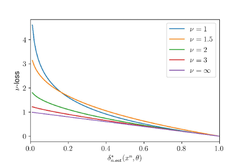
Figure 1: The plot of the $\nu$-loss $L_{\nu}(\theta,\delta^{*}_{n,\text{est}}(x^{n},\cdot))$

Proposition 5 ([7, Lem 1]).

Let $\pi$ be a prior distribution on $\theta\in\Theta$ and $r(\delta^{*}_{n,\text{est}}):=\mathbb{E}_{X^{n},\theta}\left[L_{\nu}(\theta,\delta^{*}_{n,\text{est}}(X^{n},\cdot))\right]=\sum_{x^{n},\theta}\pi(\theta)p_{X^{n}\mid\theta}(x^{n}\mid\theta)L_{\nu}(\theta,\delta_{n,\text{est}}^{*}(x^{n},\cdot))$ be Bayes risk for point estimation using a randomized decision function $\delta^{*}_{n,\text{est}}$. Then, the minimal Bayes risk is given by

$$\inf_{\delta^{*}_{n,\text{est}}}r(\delta^{*}_{n,\text{est}}) =r(\delta_{n,\text{est}}^{*,\text{Bayes}}),$$ (19)

where the optimal randomized decision function $\delta_{n,\text{est}}^{*,\text{Bayes}}\colon\mathcal{X}^{n}\times\Theta\to[0,1]$ is given as follows:

For $\nu\in[1,\infty)$,

$$\delta^{*,\text{Bayes}}_{n,\text{est}}(x^{n},\hat{\theta}) =\begin{cases}\pi(\hat{\theta}\mid x^{n}),&\nu=1,\\ \frac{\pi(\hat{\theta}\mid x^{n})^{\nu}}{\sum_{\hat{\theta}}\pi(\hat{\theta}\mid x^{n})^{\nu}}&\nu\in(1,\infty),\end{cases}$$ (20)

where $\pi(\hat{\theta}|x^{n}):=\pi(\hat{\theta})p_{X^{n}\mid\theta}(x^{n}\mid\hat{\theta})/\sum_{\theta}\pi(\theta)p_{X^{n}\mid\theta}(x^{n}\mid\theta)$ is a posterior distribution on $\theta$ given $X^{n}=x^{n}$. For $\nu=\infty$,

$$\delta^{*,\text{Bayes}}_{n}(x^{n},\hat{\theta}) =\begin{cases}1/\left\lvert\text{MAP}(x^{n})\right\rvert,&\hat{\theta}\in\text{MAP}(x^{n}),\\ 0,&\text{otherwise},\end{cases}$$ (21)

where $\text{MAP}(x^{n}):=\left\{\,\tilde{\theta}\in\Theta\mathrel{}\middle|\mathrel{}\pi(\tilde{\theta}\mid x^{n})=\max_{\theta}\pi(\theta\mid x^{n})\right\}$.

III Hypothesis Testing via a Tunable-loss

In this section, we will formulate hypothesis testing problems via the tunable-loss in both Neyman–Peason’s setting and the Bayesian setting.

Let $\Theta=\{\theta_{0},\theta_{1}\}$ be a parameter space, $\delta_{n}^{*}\colon\mathcal{X}^{n}\times\{0,1\}\to[0,1]$ be a randomized test function for hypotheses $H_{0}\colon\theta=\theta_{0}$ v.s. $H_{1}\colon\theta=\theta_{1}$, i.e., given $X^{n}=x^{n}$, $\delta_{n}^{*}(x^{n},0)$ represents the probability of accepting the null hypothesis $H_{0}$ and $\delta_{n}^{*}(x^{n},1)=1-\delta_{n}^{*}(x^{n},0)$ represents the probability of accepting the alternative hypothesis $H_{1}$ ($=$ probability of rejecting the null hypothesis $H_{0}$), respectively. Let $\Delta_{n}^{*}$ be a set of all randomized test functions. In this section, we formulate problems of the simple hypothesis testing using the randomized test and a tunable loss function. First, we define $\nu$-loss for the hypothesis testing as follows.

Definition 7 ($\nu$-loss for a test function).

For $\nu\in(1,\infty)$, $\nu$-loss for a randomized test $\delta_{n}^{*}$ is defined as follows:

$$L_{{\nu}}(\theta,\delta_{n}^{*}(x^{n},\cdot)) =\begin{cases}\frac{\nu}{\nu-1}\left\{1-\delta^{*}_{n}(x^{n},0)^{\frac{\nu-1}{\nu}}\right\},&\theta=\theta_{0},\\ \frac{\nu}{\nu-1}\left\{1-\delta^{*}_{n}(x^{n},1)^{\frac{\nu-1}{\nu}}\right\},&\theta=\theta_{1}.\end{cases}$$ (22)

The value of $L_{\nu}(\theta,\delta_{n}^{*}(x^{n},\cdot))$ is extended by continuity to $\nu=1$ (log-loss) and $\nu=\infty$ (soft $0$-$1$ loss) as Definition 6.

Remark 2.

The higher the probability $\delta_{n}^{*}(x^{n},0)$ of accepting the null hypothesis $H_{0}\colon\theta=\theta_{0}$ when it is correct, the smaller the value of the loss function. Similarly, the higher the probability $\delta_{n}^{*}(x^{n},1)=1-\delta_{n}^{*}(x^{n},0)$ of rejecting the null hypothesis when it is false, the smaller the value of the loss function.

Then we define $\nu$-Type I/II error and $\nu$-Bayesian error probability via risk function $R(\theta,\delta_{n}^{*}):=\mathbb{E}_{X^{n}\mid\theta}\left[L_{\nu}(\theta,\delta_{n}^{*}(X^{n},\cdot))\right]$ and Bayes risk function $r(\delta_{n}^{*}):=\mathbb{E}_{\theta}\left[R(\theta,\delta_{n}^{*})\right]$.

Definition 8 ($\nu$-Type I/II error, $\nu$-Bayesian error).

$$R(\theta,\delta^{*}_{n}) =\begin{cases}\alpha_{{\nu}}(\theta_{0},\delta^{*}_{n}),&\theta=\theta_{0},\\ \bar{\beta}_{{\nu}}(\theta_{1},\delta^{*}_{n}),&\theta=\theta_{1},\end{cases}$$ (23)

$$r(\delta_{n}^{*}) =\pi_{0}\alpha_{{\nu}}(\theta_{0},\delta^{*}_{n})+\pi_{1}\bar{\beta}_{{\nu}}(\theta_{1},\delta^{*}_{n}),(\text{{$\nu$}-Bayesian error})$$ (24)

where $\pi_{i}=\pi(\theta_{i}),i=0,1$ is the prior probability on $\theta=\theta_{i}$ and

$$\alpha_{{\nu}}(\theta_{0},\delta^{*}_{n}) :=\frac{\nu}{\nu-1}\left\{1-\mathbb{E}_{X^{n}\mid\theta_{0}}\left[\delta^{*}_{n}(X^{n},0)^{\frac{\nu-1}{\nu}}\right]\right\},$$

$$\qquad\qquad\qquad\qquad\qquad(\text{{$\nu$}-Type I error})$$ (25)

$$\bar{\beta}_{{\nu}}(\theta_{1},\delta^{*}_{n}) :=\frac{\nu}{\nu-1}\left\{1-\mathbb{E}_{X^{n}\mid\theta_{1}}\left[\delta^{*}_{n}(X^{n},1)^{\frac{\nu-1}{\nu}}\right]\right\}.$$

$$\qquad\qquad\qquad\qquad\qquad(\text{{$\nu$}-Type II error})$$ (26)

Based on the $\nu$-Type I/II error and $\nu$-Bayesian error, we extend the concepts in the classical hypothesis testing problem as follows.

Definition 9 ($\nu$-MP test of size $\epsilon$).

Let $\epsilon\in(0,1)$. The randomized test function $\delta_{n}^{*,\text{$\nu$-\text{MP}}}\colon\mathcal{X}^{n}\times\{0,1\}\to[0,1]$ is the $\nu$-MP test of size $\epsilon$ if the following hold:

1. $\alpha_{{\nu}}(\theta_{0},\delta_{n}^{*,{\nu}\text{-MP}})\leq\epsilon$,

2. For any randomized test $\delta^{*}_{n}\in\Delta_{n}^{*}$,
   $\alpha_{{\nu}}(\theta_{0},\delta^{*}_{n})\leq\epsilon\Longrightarrow\bar{\beta}_{{\nu}}(\theta_{1},\delta^{*}_{n})\geq\bar{\beta}_{{\nu}}(\theta_{1},\delta_{n}^{*,{\nu}\text{-MP}})$.

Definition 10 ($(\nu,\epsilon)$-error exponent).

Let $\nu\in[1,\infty]$ and $\epsilon\in(0,1)$. The $(\nu,\epsilon)$-optimal error exponent $B_{\nu,\epsilon}$ is defined as

$$B_{\nu,\epsilon} :=-\lim_{n\to\infty}\frac{1}{n}\log\inf_{\delta_{n}^{*}\colon\alpha_{\nu}(\theta_{0},\delta_{n}^{*})<\epsilon}\bar{\beta}(\theta_{1},\delta_{n}^{*}),$$ (27)

where infimum is over all randomized test functions $\delta_{n}^{*}$ satisfying $\alpha_{\nu}(\theta_{0},\delta_{n}^{*})<\epsilon$.

Definition 11 ($\nu$-Bayesian error exponent).

Let $\nu\in[1,\infty]$. The $\nu$-Bayesian error exponent $D_{\nu}^{*}$ is defined as

$$D_{\nu}^{*} :=-\lim_{n\to\infty}\frac{1}{n}\log\inf_{\delta_{n}^{*}\in\Delta_{n}^{*}}r(\delta_{n}^{*}).$$ (28)

IV Main Results

The main results of this paper are derivations of the $\nu$-MP test, characterization of the $(\nu,\epsilon)$-error exponent, and derivation of lower bounds of the $\nu$-Bayesian error exponent.

Theorem 1.

Let $\epsilon\in(0,1)$. The $\nu$-MP test of size $\epsilon$ is given as follows:
For $\nu\in[1,\infty)$,

$$\delta^{*,\text{$\nu$-MP}}(x^{n},1) =\frac{\lambda^{-{\nu}}p_{X^{n}\mid\theta}(x^{n}\mid\theta_{0})^{-{\nu}}}{p_{X^{n}\mid\theta}(x^{n}\mid\theta_{1})^{-{\nu}}+\lambda^{-{\nu}}p_{X^{n}\mid\theta}(x^{n}\mid\theta_{0})^{-{\nu}}},$$ (29)

$$\delta^{*,\text{$\nu$-MP}}(x^{n},0) =1-\delta^{*,\text{$\nu$-MP}}(x^{n},1).$$ (30)

For $\nu=\infty$,

$$\delta^{*,\text{$\infty$-MP}}(x^{n},1) =\begin{cases}1,&\frac{p_{X^{n}\mid\theta}(x^{n}\mid\theta_{0})}{p_{X^{n}\mid\theta}(x^{n}\mid\theta_{1})}\leq\lambda\\ 0,&\text{otherwise},\end{cases}$$ (31)

$$\delta^{*,\text{$\infty$-MP}}(x^{n},0) =1-\delta^{*,\text{$\infty$-MP}}(x^{n},1).$$ (32)

Note that $\lambda$ is determined such that $\alpha_{\nu}(\theta_{0},\delta_{n}^{\text{$\nu$-MP}})=\epsilon$ for $\nu\in[1,\infty]$.

Remark 3.

Note that the $\infty$-MP test (31)(32) corresponds to the likelihood test defined in (8).

Proof.

See Appendix A. ∎

Theorem 2.

For any $\epsilon\in(0,1)$ and any $\nu\in[1,\infty]$,

$$B_{{\nu},\epsilon} =D(p_{X\mid\theta_{0}}||p_{X\mid\theta_{1}}),$$ (33)

where $D(p_{X\mid\theta_{0}}||p_{X\mid\theta_{1}})$ is the Kullback–Leibler divergence.

Remark 4.

The $(\nu,\epsilon)$-error exponent does not depend on $\nu$ as well as $\epsilon$.

Proof.

See Appendix B. ∎

Proposition 6.

The minimal $\nu$-Bayesian error probability is given by

$$\inf_{\delta_{n}^{*}}r(\delta_{n}^{*})=r(\delta_{n}^{*,\text{Bayes}}),$$

where the optimal randomized test function $\delta_{n}^{*,\text{Bayes}}\colon\mathcal{X}^{n}\times\{0,1\}\to[0,1]$ is given as follows:
For $\nu\in[1,\infty)$,

$$\delta_{n}^{*,\text{Bayes}}(x^{n},0) :=\frac{\pi(\theta_{0}\mid x^{n})^{\nu}}{\pi(\theta_{0}\mid x^{n})^{\nu}+\pi(\theta_{1}\mid x^{n})^{\nu}},$$ (34)

$$\delta_{n}^{*,\text{Bayes}}(x^{n},1) :=1-\delta_{n}^{*,\text{Bayes}}(x^{n},0).$$ (35)

For $\nu=\infty$,

$$\delta_{n}^{*,\text{Bayes}}(x^{n},0) =\begin{cases}1,&\pi(\theta_{0}\mid x^{n})\geq\pi(\theta_{1}\mid x^{n}),\\ 0,&\text{otherwise},\end{cases}$$ (36)

$$\delta_{n}^{*,\text{Bayes}}(x^{n},1) =1-\delta_{n}^{*,\text{Bayes}}(x^{n},0),$$ (37)

where $\pi(\theta_{i}\mid x^{n}):=\pi_{i}p_{X^{n}\mid\theta}(x^{n}\mid\theta_{i})/\sum_{i=0}^{1}\pi_{i}p(x^{n}\mid\theta_{i})$.

Proof.

It can be proved in a similar way as Proposition 5 (see [7, Appendix A]). ∎

Theorem 3.

$$D_{\nu}^{*} \begin{cases}\geq D_{\text{B},\nu}(p_{X\mid\theta_{0}},p_{X\mid\theta_{1}}),&\nu\in[1,\infty),\\ =C(p_{X\mid\theta_{0}},p_{X\mid\theta_{1}}),&\nu=\infty,\end{cases}$$ (38)

where $D_{\text{B},\nu}(p_{X\mid\theta_{0}},p_{X\mid\theta_{1}})$ is defined as

$$D_{\text{B},\nu}(p_{X\mid\theta_{0}},p_{X\mid\theta_{1}}):=-\log\max\{\text{BC}_{{\nu}/{2}},\text{BC}_{1-{\nu}/{2}}\},$$ (39)

$$\text{BC}_{{\nu}/{2}}:=\sum_{x}{p_{X\mid\theta}(x\mid\theta_{0})^{\frac{\nu}{2}}p_{X\mid\theta}(x\mid\theta_{1})^{1-\frac{\nu}{2}}},$$ (40)

and $C(p_{X\mid\theta_{0}},p_{X\mid\theta_{1}})$ is the Chernoff-information defined in (17).

Remark 5.

$\text{BC}_{{\nu}/{2}}$ is called the $\frac{\nu}{2}$-skewed Bhattacharyya affinity coefficient [15]. Note that $D_{\text{B},1}$ and $\text{BC}_{1/2}$ equal the Bhattacharyya distance and the Bhattacharyya coefficient, respectively.

Proof.

See Appendix C. ∎

Basic properties of the lower bound $D_{\text{B},\nu}(p_{X\mid\theta_{0}},p_{X\mid\theta_{1}})$ follows immediately from [16, Exercise 2.28] and [17, Cor 2].

Corollary 1.

The following hold:

1. $D_{\text{B},\nu}(p_{X\mid\theta_{0}},p_{X\mid\theta_{1}})$ is concave in $\nu\in[1,\infty)$.

2. $D_{\text{B},\nu}(p_{X\mid\theta_{0}},p_{X\mid\theta_{1}})\geq 0$ for $\nu\in[1,2)$,

3. $D_{\text{B},\nu}(p_{X\mid\theta_{0}},p_{X\mid\theta_{1}})=0$ for $\nu=2$,

4. $D_{\text{B},\nu}(p_{X\mid\theta_{0}},p_{X\mid\theta_{1}})<0$ for $\nu\in(2,\infty)$.

Note that when $\nu\geq 2$, this lower bound $D_{\text{B},\nu}(p_{X\mid\theta_{0}},p_{X\mid\theta_{1}})$ is useless.

Example 1.

Let $X^{n}=(X_{1},\dots,X_{n})$ be a random sample of size $n$ from the Bernoulli distribution $\textsf{Bern}(\theta)$. Now, consider the following hypothesis test:

$$H_{0}:\theta=0.5\text{ vs. }H_{1}:\theta=0.7.$$

In this situation, Figure 2 shows a graph of the lower bound $D_{\text{B},\nu}$ for $\nu\in[1,2]$.

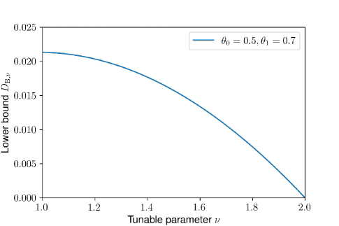
Figure 2: The plot of the lower bound $D_{\text{B},\nu}$ as a function of $\nu$

V Conclusion

In this work, we have developed simple hypothesis testing problems via the tunable loss by Liao et al.[7] in the Neyman–Pearsons’ and Bayesian settings. Our results correspond to Neyman–Pearson lemma, Chernoff-Stein lemma, and Chernoff-information. Future work includes deriving upper bound of $\nu$-Bayesian error exponent $D^{*}_{\nu}$ and valid lower bound for $\nu\geq 2$.

Appendix A Proof of Theorem 1

Proof.

For $\nu=\infty$, it can be proved in the same way as for the Neyman–Pearson lemma by considering the set $\textsf{A}(\delta^{*,\text{$\infty$-MP}}_{n}):=\left\{\,x^{n}\in\mathcal{X}^{n}\mathrel{}\middle|\mathrel{}\delta^{*,\text{$\infty$-MP}}_{n}(x^{n},0)=1\right\}$ to be an acceptance region. For $\nu\in(1,\infty)$, the $\nu$-MP test $\delta^{*,\text{$\nu$-MP}}$ is the solution to the following optimization problem:

$$\text{minimize }\bar{\beta}_{{\nu}}(\theta_{1},\delta^{*}_{n})=\frac{\nu}{\nu-1}\left\{1-\mathbb{E}_{X^{n}\mid\theta_{1}}\left[\delta^{*}_{n}(X^{n},1)^{\frac{\nu-1}{\nu}}\right]\right\}$$

subject to

$$\alpha_{{\nu}}(\theta_{0},\delta^{*}_{n})=\frac{\nu}{\nu-1}\left\{1-\mathbb{E}_{X^{n}\mid\theta_{0}}\left[\delta^{*}_{n}(X^{n},0)^{\frac{\nu-1}{\nu}}\right]\right\}\leq\epsilon$$

$$0\leq\delta^{*}_{n}(x^{n},0)\leq 1,$$

$$0\leq\delta^{*}_{n}(x^{n},1)\leq 1,$$

$$\delta^{*}_{n}(x^{n},0)+\delta^{*}_{n}(x^{n},1)=1.$$

By using the KKT conditions, we obtain (29)(30). For $\nu=1$, it can be proved in a similar way as $\nu\in(1,\infty)$. ∎

Appendix B Proof of Theorem 2

Proof.

We will prove only for $\nu\in(1,\infty)$. Proofs for $\nu=1$ and $\nu=\infty$ can be obtained in a similar way. For simplicity, we will denote $D(p_{X\mid\theta_{0}}||p_{X\mid\theta_{1}})$ by $D(p_{0}||p_{1})$.

(Direct part): Let $\epsilon^{\prime}>0$ be an arbitrarily small number such that $0<\epsilon^{\prime}<\epsilon$ and $\epsilon^{\prime}_{{\nu}}:=\epsilon^{\prime}({\nu}-1)/{\nu}$. Define a set of $\epsilon_{\nu}^{\prime}$-relative typical sequences $A_{\epsilon_{\nu}^{\prime}}^{(n)}(p_{{0}}||p_{{1}})$ as follows:

$$A_{\epsilon_{\nu}^{\prime}}^{(n)}(p_{{0}}||p_{{1}})$$

$$:=\left\{\,x^{n}\in\mathcal{X}^{n}\colon\left\lvert\frac{1}{n}\log\frac{p_{X\mid\theta}(x^{n}\mid\theta_{0})}{p_{X\mid\theta}(x^{n}\mid\theta_{1})}-D(p_{0}||p_{1})\right\rvert\leq\epsilon_{\nu}^{\prime}\right\}.$$ (41)

Moreover, define a sequence of test functions $(\delta_{n}^{*,\text{AEP}})_{n=1}^{\infty}$ as follows:

$$\delta_{n}^{*,\text{AEP}}(x^{n},1) =\begin{cases}0,&x^{n}\in A_{\epsilon_{\nu}^{\prime}}^{(n)}(p_{{0}}||p_{{1}}),\\ 1,&\text{otherwise}.\end{cases}$$ (42)

Then, from the asymptotic equipartition property (AEP, see, [5, Thm 11.8.2]), the following holds for sufficiently large $n$:

$$\alpha_{{\nu}}(\theta_{0},\delta_{n}^{*,\text{AEP}})$$

$$=\frac{\nu}{\nu-1}\Bigl{\{}1-\sum_{x^{n}}p_{X^{n}\mid\theta}(x^{n}\mid\theta_{0})\delta^{*,\text{AEP}}(x^{n},0)^{\frac{\nu-1}{\nu}}\Bigr{\}}$$ (43)

$$=\frac{\nu}{\nu-1}\cdot\underbrace{\sum_{x^{n}\in A_{\epsilon_{\nu}^{\prime}}^{(n)^{c}}}(p_{0}||p_{1})p_{X^{n}\mid\theta}(x^{n}\mid\theta_{0})}_{\leq\epsilon_{\nu}^{\prime}}$$ (44)

$$\leq\frac{\nu}{\nu-1}\cdot\epsilon_{\nu}^{\prime}=\epsilon^{\prime}\leq\epsilon.$$ (45)

Similarly, it also holds from the AEP that

$$-\lim_{n\to\infty}\frac{1}{n}\log\bar{\beta}_{{\nu}}(\theta_{1},\delta_{n}^{*,\text{AEP}})$$

$$=-\lim_{n\to\infty}\frac{1}{n}\log\frac{\nu}{\nu-1}\cdot\underbrace{\sum_{x^{n}\in A_{\epsilon_{\nu}^{\prime}}^{(n)}(p_{0}||p_{1})}p_{X^{n}\mid\theta}(x^{n}\mid\theta_{1})}_{<2^{-n(D(p_{0}||p_{1})-\epsilon_{\nu}^{\prime})}}$$ (46)

$$\geq D(p_{0}||p_{1})-\epsilon_{\nu}^{\prime}>D(p_{0}||p_{1})-\epsilon^{\prime}.$$ (47)

Therefore, $R=D(p_{0}||p_{1})-\epsilon^{\prime}$ is achievable. Since $\epsilon^{\prime}>0$ is arbitrary, we can conclude that $B_{\nu,\epsilon}\geq D(p_{0}||p_{1})$.

(Converse part): Let $\epsilon^{\prime}>0$ be an arbitrarily small number such that $0<\epsilon^{\prime}<\epsilon$ and $(\delta^{*}_{n})_{n=1}^{\infty}$ be an arbitrary sequence of randomized test functions such that $\alpha_{{\nu}}(\theta_{0},\delta^{*}_{n})\leq\epsilon^{\prime}$ for sufficiently large $n$. Let $A_{\epsilon^{\prime}}^{(n)}(p_{0}||p_{1})$ be an $\epsilon^{\prime}$-relative typical sequences. First, we will show the next lemma by using the Jensen’s inequality.

Lemma 1.

$$\sum_{x^{n}\in A_{\epsilon^{\prime}}^{(n)}(p_{0}||p_{1})}p_{X^{n}\mid\theta}(x^{n}\mid\theta_{0})\delta^{*}_{n}(x^{n},0)\geq 1-2\epsilon^{\prime}.$$ (48)

Proof.

Since

$$\alpha_{{\nu}}(\theta_{0},\delta^{*}_{n}) :=\frac{\nu}{\nu-1}\left\{1-\mathbb{E}_{X^{n}\mid\theta_{0}}\left[\delta^{*}_{n}(X^{n},0)^{\frac{\nu-1}{\nu}}\right]\right\}\leq\epsilon^{\prime}$$ (49)

for sufficiently large $n$, it holds that

$$\mathbb{E}_{X^{n}\mid\theta_{0}}\left[\delta^{*}_{n}(X^{n},0)^{\frac{\nu-1}{\nu}}\right]\geq 1-\frac{\nu-1}{\nu}\cdot\epsilon^{\prime}.$$ (50)

Then, it follows from the Jensen’s inequality that

$$\left\{\mathbb{E}_{X^{n}\mid\theta_{0}}\left[\delta^{*}_{n}(X^{n},0)\right]\right\}^{\frac{\nu-1}{\nu}} \geq\mathbb{E}_{X^{n}\mid\theta_{0}}\left[\delta^{*}_{n}(X^{n},0)^{\frac{\nu-1}{\nu}}\right]$$ (51)

$$\geq 1-\frac{\nu-1}{\nu}\cdot\epsilon^{\prime}.$$ (52)

Thus, we have

$$\mathbb{E}_{X^{n}\mid\theta_{0}}\left[\delta^{*}_{n}(X^{n},0)\right] \geq\left(1-\frac{\nu-1}{\nu}\cdot\epsilon^{\prime}\right)^{\frac{\nu}{\nu-1}}$$ (53)

$$\overset{(a)}{\geq}1-\epsilon^{\prime},$$ (54)

where

• $(a)$ follows from $(1-\gamma x)^{1/\gamma}\geq 1-x$ for $0<\gamma\leq 1,0\leq x\leq 1$.

From the AEP, $\mathbb{E}_{X^{n}\mid\theta_{0}}\left[\delta^{*}_{n}(X^{n},0)\right]$ can be upper bounded as follows:

$$\mathbb{E}_{X^{n}\mid\theta_{0}}\left[\delta^{*}_{n}(X^{n},0)\right]$$

$$=\sum_{x^{n}\in A_{\epsilon^{\prime}}^{(n)}(p_{0}||p_{1})}p_{X^{n}\mid\theta}(x^{n}\mid\theta_{0})\delta^{*}_{n}(x^{n},0)$$

$$\qquad+\sum_{x^{n}\in A_{\epsilon^{\prime}}^{(n)^{c}}(p_{0}||p_{1})}p_{X^{n}\mid\theta}(x^{n}\mid\theta_{0})\delta^{*}_{n}(x^{n},0)$$ (55)

$$\leq\sum_{x^{n}\in A_{\epsilon^{\prime}}^{(n)}(p_{0}||p_{1})}p_{X^{n}\mid\theta}(x^{n}\mid\theta_{0})\delta^{*}_{n}(x^{n},0)$$

$$\qquad+\underbrace{\sum_{x^{n}\in A_{\epsilon^{\prime}}^{(n)^{c}}(p_{0}||p_{1})}p_{X^{n}\mid\theta}(x^{n}\mid\theta_{0})}_{\leq\epsilon^{\prime}}$$ (56)

$$\leq\sum_{x^{n}\in A_{\epsilon^{\prime}}^{(n)}(p_{0}||p_{1})}p_{X^{n}\mid\theta}(x^{n}\mid\theta_{0})\delta^{*}_{n}(x^{n},0)+\epsilon^{\prime}.$$ (57)

Therefore, $\sum_{x^{n}\in A_{\epsilon^{\prime}}^{(n)}(p_{0}||p_{1})}p_{X^{n}\mid\theta}(x^{n}\mid\theta_{0})\delta^{*}_{n}(x^{n},0)\geq 1-2\epsilon^{\prime}$. ∎

Next, $\bar{\beta}_{{\nu}}(\theta_{1},\delta^{*}_{n})$ can be lower bounded as follows:

$$\bar{\beta}_{{\nu}}(\theta_{1},\delta^{*}_{n})$$

$$:=\frac{\nu}{\nu-1}\left\{1-\sum_{x^{n}}p_{X^{n}\mid\theta}(x^{n}\mid\theta_{1})\delta^{*}_{n}(x^{n},1)^{\frac{\nu-1}{\nu}}\right\}$$ (58)

$$=\frac{\nu}{\nu-1}\left\{1-\sum_{x^{n}}p_{X^{n}\mid\theta}(x^{n}\mid\theta_{1})(1-\delta^{*}_{n}(x^{n},0))^{\frac{\nu-1}{\nu}}\right\}$$ (59)

$$\overset{(b)}{\geq}\frac{\nu}{\nu-1}\left\{1+\sum_{x^{n}}p_{X^{n}\mid\theta}(x^{n}|\theta_{1})\left(-1+\frac{\nu-1}{\nu}\delta^{*}_{n}(x^{n},0)\right)\right\}$$ (60)

$$=\sum_{x^{n}}p_{X^{n}\mid\theta}(x^{n}\mid\theta_{1})\delta^{*}_{n}(x^{n},0),$$ (61)

where

• $(b)$ follows from $(1-x)^{\gamma}\leq 1-\gamma x$, for $0<\gamma\leq 1,0\leq x\leq 1$.

Making use of the result in Lemma 1 and AEP, we have

$$\sum_{x^{n}}p_{X^{n}\mid\theta}(x^{n}\mid\theta_{1})\delta^{*}_{n}(x^{n},0)$$

$$\geq\sum_{x^{n}\in A_{\epsilon^{\prime}}^{(n)}(p_{0}||p_{1})}\underbrace{p_{X^{n}\mid\theta}(x^{n}\mid\theta_{1})}_{\qquad\geq p_{X^{n}\mid\theta}(x^{n}\mid\theta_{0})2^{-n(D(p_{0}||p_{1})+\epsilon^{\prime})}}\delta^{*}_{n}(x^{n},0)$$

$$\geq 2^{-n(D(p_{0}||p_{1})+\epsilon^{\prime})}\sum_{x^{n}\in A_{\epsilon^{\prime}}^{(n)}(p_{0}||p_{1})}p_{x^{n}\mid\theta}(x^{n}\mid\theta_{0})\delta^{*}_{n}(x^{n},0)$$

$$\geq 2^{-n(D(p_{0}||p_{1})+\epsilon^{\prime})}(1-2\epsilon^{\prime}).$$

Therefore, we have $-\liminf_{n\to\infty}\frac{1}{n}\log\bar{\beta}_{{\nu}}(\theta_{1},\delta^{*}_{n})\leq D(p_{0}||p_{1})+\epsilon^{\prime}$. Since $\epsilon^{\prime}>0$ is arbitrary, we can conclude that $B_{\nu,\epsilon}\leq D(p_{0}||p_{1})$. ∎

Appendix C Proof of Theorem 3

Proof.

From Proposition 6, for $\nu=\infty$, the $\infty$-Bayesian error probability is given as

$$r(\delta_{n}^{*,\text{Bayes}})=\pi_{0}\sum_{x^{n}\in\textsf{A}(\delta_{n}^{*,\text{Bayes}})}p_{X^{n}\mid\theta}(x^{n}\mid\theta_{0})$$

$$\qquad+\pi_{1}\sum_{x^{n}\in\textsf{A}(\delta_{n}^{*,\text{Bayes}})^{c}}p_{X^{n}\mid\theta}(x^{n}\mid\theta_{1}),$$ (62)

where $\textsf{A}(\delta_{n}^{*,\text{Bayes}}):=\left\{\,x^{n}\in\mathcal{X}^{n}\mathrel{}\middle|\mathrel{}\pi(\theta_{0}\mid x^{n})\geq\pi(\theta_{1}\mid x^{n})\right\}$. Thus the problem of characterizing $\infty$-Bayesian error exponent $D_{\infty}^{*}$ is equivalent to the classical problem of characterizing the Bayesian error exponent $D^{*}$ defined in (15). Therefore, $D_{\infty}^{*}=C(p_{X\mid\theta_{0}},p_{X\mid\theta_{1}})$ (see [5]).

For $\nu\in(1,\infty)$, the $\nu$-Bayesian error probability is given, and upper bounded as follows:

$$r(\delta_{n}^{*,\text{Bayes}})=\pi_{0}\cdot\frac{\nu}{\nu-1}\cdot\sum_{x^{n}}p_{X^{n}\mid\theta}(x^{n}\mid\theta_{0})$$

$$\times\left\{1-\left(\frac{\pi(\theta_{0}\mid x^{n})^{\nu}}{\pi(\theta_{0}\mid x^{n})^{\nu}+\pi(\theta_{1}\mid x^{n})^{\nu}}\right)^{\frac{\nu-1}{\nu}}\right\}$$

$$+\pi_{1}\cdot\frac{\nu}{\nu-1}\cdot\sum_{x^{n}}p_{X^{n}\mid\theta}(x^{n}\mid\theta_{1})$$

$$\times\left\{1-\left(\frac{\pi(\theta_{1}\mid x^{n})^{\nu}}{\pi(\theta_{0}\mid x^{n})^{\nu}+\pi(\theta_{1}\mid x^{n})^{\nu}}\right)^{\frac{\nu-1}{\nu}}\right\}$$ (63)

$$\overset{(a)}{\leq}\pi_{0}\cdot\frac{\nu}{\nu-1}\cdot\sum_{x^{n}}p_{X^{n}\mid\theta}(x^{n}\mid\theta_{0})$$

$$\times\left\{1-\frac{\pi(\theta_{0}\mid x^{n})^{\nu}}{\pi(\theta_{0}\mid x^{n})^{\nu}+\pi(\theta_{1}\mid x^{n})^{\nu}}\right\}$$

$$+\pi_{1}\cdot\frac{\nu}{\nu-1}\cdot\sum_{x^{n}}p_{X^{n}\mid\theta}(x^{n}\mid\theta_{1})$$

$$\times\left\{1-\frac{\pi(\theta_{1}\mid x^{n})^{\nu}}{\pi(\theta_{0}\mid x^{n})^{\nu}+\pi(\theta_{1}\mid x^{n})^{\nu}}\right\}$$ (64)

$$=\frac{\nu}{\nu-1}\cdot\sum_{x^{n}}\frac{\pi_{0}p_{X^{n}\mid\theta}(x^{n}\mid\theta_{0})\pi_{1}^{\nu}p_{X^{n}\mid\theta}(x^{n}\mid\theta_{1})^{\nu}}{\pi_{0}^{\nu}p_{X^{n}\mid\theta}(x^{n}\mid\theta_{0})^{\nu}+\pi_{1}^{\nu}p_{X^{n}\mid\theta}(x^{n}\mid\theta_{1})^{\nu}}$$

$$+\frac{\nu}{\nu-1}\cdot\sum_{x^{n}}\frac{\pi_{1}p_{X^{n}\mid\theta}(x^{n}\mid\theta_{1})\pi_{0}^{\nu}p_{X^{n}\mid\theta}(x^{n}\mid\theta_{0})^{\nu}}{\pi_{0}^{\nu}p_{X^{n}\mid\theta}(x^{n}\mid\theta_{0})^{\nu}+\pi_{1}^{\nu}p_{X^{n}\mid\theta}(x^{n}\mid\theta_{1})^{\nu}}$$ (65)

$$=\frac{\nu}{\nu-1}\cdot\sum_{x^{n}}\frac{1}{\frac{\pi_{0}^{\nu-1}p_{X^{n}\mid\theta}(x^{n}\mid\theta_{0})^{\nu-1}}{\pi_{1}^{\nu}p_{X^{n}\mid\theta}(x^{n}\mid\theta_{1})^{\nu}}+\frac{1}{\pi_{0}p_{X^{n}\mid\theta}(x^{n}\mid\theta_{0})}}$$

$$+\frac{\nu}{\nu-1}\cdot\sum_{x^{n}}\frac{1}{\frac{\pi_{1}^{\nu-1}p_{X^{n}\mid\theta}(x^{n}\mid\theta_{1})^{\nu-1}}{\pi_{0}^{\nu}p_{X^{n}\mid\theta}(x^{n}\mid\theta_{0})^{\nu}}+\frac{1}{\pi_{1}p_{X^{n}\mid\theta}(x^{n}\mid\theta_{1})}}$$ (66)

$$\overset{(b)}{\leq}\frac{1}{2}\cdot\frac{\nu}{\nu-1}\sum_{x^{n}}(\pi_{1}p_{X^{n}\mid\theta}(x^{n}\mid\theta_{1}))^{\frac{\nu}{2}}(\pi_{0}p_{X^{n}\mid\theta}(x^{n}\mid\theta_{0}))^{1-\frac{\nu}{2}}$$

$$+\frac{1}{2}\cdot\frac{\nu}{\nu-1}\sum_{x^{n}}(\pi_{0}p_{X^{n}\mid\theta}(x^{n}\mid\theta_{0}))^{\frac{\nu}{2}}(\pi_{1}p_{X^{n}\mid\theta}(x^{n}\mid\theta_{1}))^{1-\frac{\nu}{2}}$$ (67)

$$=\frac{1}{2}\cdot\frac{\nu}{\nu-1}\cdot\pi_{1}^{\frac{\nu}{2}}\pi_{0}^{1-\frac{\nu}{2}}\sum_{x^{n}}\prod_{i=1}^{n}p_{X\mid\theta}(x_{i}\mid\theta_{1})^{\frac{\nu}{2}}p_{X\mid\theta}(x_{i}\mid\theta_{0})^{1-\frac{\nu}{2}}$$

$$+\frac{1}{2}\cdot\frac{\nu}{\nu-1}\cdot\pi_{0}^{\frac{\nu}{2}}\pi_{1}^{1-\frac{\nu}{2}}\sum_{x^{n}}\prod_{i=1}^{n}p_{X\mid\theta}(x_{i}\mid\theta_{0})^{\frac{\nu}{2}}p_{X\mid\theta}(x_{i}\mid\theta_{1})^{1-\frac{\nu}{2}}$$ (68)

$$=\frac{1}{2}\cdot\frac{\nu}{\nu-1}\cdot\pi_{1}^{\frac{\nu}{2}}\pi_{0}^{1-\frac{\nu}{2}}\left(\sum_{x}p_{X\mid\theta}(x\mid\theta_{1})^{\frac{\nu}{2}}p_{X\mid\theta}(x\mid\theta_{0})^{1-\frac{\nu}{2}}\right)^{n}$$

$$+\frac{1}{2}\cdot\frac{\nu}{\nu-1}\cdot\pi_{0}^{\frac{\nu}{2}}\pi_{1}^{1-\frac{\nu}{2}}\left(\sum_{x}p_{X\mid\theta}(x\mid\theta_{0})^{\frac{\nu}{2}}p_{X\mid\theta}(x\mid\theta_{1})^{1-\frac{\nu}{2}}\right)^{n}$$ (69)

$$\overset{(c)}{\leq}\frac{\nu}{\nu-1}\max\Bigl{\{}\sum_{x}p_{X\mid\theta}(x\mid\theta_{1})^{\frac{\nu}{2}}p_{X\mid\theta}(x\mid\theta_{0})^{1-\frac{\nu}{2}},$$

$$\qquad\qquad\qquad\sum_{x}p_{X\mid\theta}(x\mid\theta_{0})^{\frac{\nu}{2}}p_{X\mid\theta}(x\mid\theta_{1})^{1-\frac{\nu}{2}}\Bigr{\}}^{n},$$ (70)

where

• $(a)$ follows from $1-x^{\gamma}\leq 1-x$ for $0\leq\gamma\leq 1$,

• $(b)$ follows from $\text{(harmonic mean)}\leq\text{(geometric mean)}$,

• $(c)$ follows from $a^{n}+b^{n}\leq 2\max\{a,b\}^{n}$ for $a,b\geq 0$ and $\pi_{0},\pi_{1}\leq 1$.

Therefore,

$$D_{\nu}^{*} =-\lim_{n\to\infty}\frac{1}{n}\log r(\delta_{n}^{*,\text{Bayes}})$$ (71)

$$\geq-\log\max\{\text{BC}_{{\nu}/{2}},\text{BC}_{1-{\nu}/{2}}\}.$$ (72)

For $\nu=1$, it can be proved in a similar way as $\nu\in(1,\infty)$ by using the inequality $1-1/x\leq\log x$. ∎

References

- [1] J. Neyman and E. S. Pearson, “The testing of statistical hypotheses in relation to probabilities a priori,” Mathematical Proceedings of the Cambridge Philosophical Society, vol. 29, no. 4, pp. 492–510, 1933.
- [2] ——, “On the problem of the most efficient tests of statistical hypotheses,” Philosophical Transactions of the Royal Society of London. Series A, Containing Papers of a Mathematical or Physical Character, vol. 231, pp. 289–337, 1933. [Online]. Available: http://www.jstor.org/stable/91247
- [3] H. Chernoff, “Large-Sample Theory: Parametric Case,” The Annals of Mathematical Statistics, vol. 27, no. 1, pp. 1 – 22, 1956. [Online]. Available: https://doi.org/10.1214/aoms/1177728347
- [4] ——, “A Measure of Asymptotic Efficiency for Tests of a Hypothesis Based on the sum of Observations,” The Annals of Mathematical Statistics, vol. 23, no. 4, pp. 493 – 507, 1952. [Online]. Available: https://doi.org/10.1214/aoms/1177729330
- [5] T. M. Cover and J. A. Thomas, Elements of Information Theory (Wiley Series in Telecommunications and Signal Processing). Wiley-Interscience, 2006.
- [6] A. Wald, “Statistical Decision Functions,” The Annals of Mathematical Statistics, vol. 20, no. 2, pp. 165 – 205, 1949. [Online]. Available: https://doi.org/10.1214/aoms/1177730030
- [7] J. Liao, O. Kosut, L. Sankar, and F. du Pin Calmon, “Tunable measures for information leakage and applications to privacy-utility tradeoffs,” IEEE Transactions on Information Theory, vol. 65, no. 12, pp. 8043–8066, 2019.
- [8] T. Sypherd, M. Diaz, L. Sankar, and P. Kairouz, “A tunable loss function for binary classification,” in 2019 IEEE International Symposium on Information Theory (ISIT), 2019, pp. 2479–2483.
- [9] T. Sypherd, M. Diaz, L. Sankar, and G. Dasarathy, “On the -loss landscape in the logistic model,” in 2020 IEEE International Symposium on Information Theory (ISIT), 2020, pp. 2700–2705.
- [10] T. Sypherd, M. Diaz, J. K. Cava, G. Dasarathy, P. Kairouz, and L. Sankar, “A tunable loss function for robust classification: Calibration, landscape, and generalization,” IEEE Transactions on Information Theory, pp. 1–1, 2022.
- [11] G. R. Kurri, T. Sypherd, and L. Sankar, “Realizing gans via a tunable loss function,” in 2021 IEEE Information Theory Workshop (ITW), 2021, pp. 1–6.
- [12] G. R. Kurri, M. Welfert, T. Sypherd, and L. Sankar, “-gan: Convergence and estimation guarantees,” 2022. [Online]. Available: https://arxiv.org/abs/2205.06393
- [13] G. R. Kurri, O. Kosut, and L. Sankar, “Evaluating multiple guesses by an adversary via a tunable loss function,” in 2021 IEEE International Symposium on Information Theory (ISIT), 2021, pp. 2002–2007.
- [14] J. Berger, Statistical decision theory and Bayesian analysis, 2nd ed., ser. Springer series in statistics. New York, NY: Springer, 1985.
- [15] F. Nielsen, “Revisiting chernoff information with likelihood ratio exponential families,” 2022. [Online]. Available: https://arxiv.org/abs/2207.03745
- [16] T. S. Han and K. Kobayashi, Mathematics of Information and Coding, ser. Translations of Mathematical Monographs. American Mathematical Society, 2002, vol. 203.
- [17] T. van Erven and P. Harremos, “Rényi divergence and kullback-leibler divergence,” IEEE Transactions on Information Theory, vol. 60, no. 7, pp. 3797–3820, 2014.