Influence of turbulence on Lyman-alpha scattering

Abstract

We develop a Monte Carlo radiative transfer code to study the effect of turbulence with a finite correlation length on scattering of Lyman-alpha (Ly$\alpha$) photons propagating through neutral atomic hydrogen gas. We investigate how the effective mean free path, the emergent spectrum, and the average number of scatterings that Ly$\alpha$ photons experience change in the presence of turbulence. We find that the correlation length is an important and sensitive parameter that has an influence on physically relevant properties of Ly$\alpha$ radiative transfer. In particular, it can significantly, by orders of magnitude, reduce the number of scattering events that the average Ly$\alpha$ photon undergoes before it escapes the turbulent cloud.

1 Introduction

The resonant Lyman-alpha (Ly$\alpha$) scattering generates a number of phenomena that are of interest in astrophysics and cosmology. Ly$\alpha$ emitters are a unique and powerful tool to learn about structure formation during the epoch of reionization (McQuinn et al., 2007; Dijkstra, 2014; Hayes, 2015; Behrens et al., 2019; Ouchi et al., 2020). Studying Ly$\alpha$ emission, propagation, and absorption allows one to constrain the ionization state of the universe, probe galaxies kinematics and dynamics, and deduce properties of the atomic gas surrounding them (Erb et al., 2018; Hayes, 2015; Wolfe et al., 2005; Ouchi et al., 2020).

The resonant scattering of Ly$\alpha$ photons through regions of neutral hydrogen (HI regions) of the intergalactic (IGM) and interstellar (ISM) media is a process which is random both in frequency and physical spaces. Except for certain cases when analytical solutions are available (Adams, 1972; Harrington, 1973; Neufeld, 1990; Loeb & Rybicki, 1999; Dijkstra et al., 2006a), one has to resort to numerical methods to study the propagation of Ly$\alpha$ radiation in these systems. The most efficient and hence popular way is to use Monte Carlo radiative transfer simulations (Dijkstra et al., 2006a, b; Dijkstra, 2014; Laursen et al., 2009; Laursen, 2010; Zheng & Miralda-Escude, 2002; Zheng & Wallace, 2014; Semelin, B. et al., 2007; Smith et al., 2018, 2020; Seon & Kim, 2020; Seon et al., 2022). The influence of many effects on the propagation of Ly$\alpha$ photons has been studied, but the effect of unresolved turbulence has received much less attention. Meanwhile, at least in some of the Ly$\alpha$ emitters the photon escape is believed to be driven by turbulence in the star-forming gas (Puschnig, J. et al., 2020). The extraction of the ISM turbulence parameters from the observations requires combination of different techniques – statistical methods and comparison with the simulations – that allow for disentanglement of the velocity and density information. The most common statistical parameters used for describing the turbulence are the slopes of velocity and density power spectra. These numbers vary from -2.0 to -1.4 and from -1.6 to -0.4 correspondingly for the observed systems (e.g. Burkhart 2021). The power law behavior cuts off at Kolmogorov length scale, for instance in the observation of the Taurus molecular cloud the HI velocity spectrum cuts off at 0.3 pc, but the turbulent cascade continues in H2 (Yuen et al., 2022).

Usually turbulence in Monte Carlo radiative transfer codes is treated as an effective thermal velocity that changes the Doppler broadening parameter from $b=v_{\textrm{th}}$ to $b=\sqrt{v_{\textrm{th}}^{2}+v_{\textrm{turb}}^{2}}$ (Eastman & MacAlpine, 1985; Ben Jaffel et al., 1993; Smith et al., 2022). This corresponds to the so-called model of microturbulence. However, besides its amplitude ($v_{\textrm{turb}}$), turbulence has another crucial parameter – the correlation length ($l_{\textrm{turb}}$). Such turbulence with a finite correlation length is often referred to as macroturbulence. In principle, it is possible to execute Monte Carlo radiative transfer codes along with hydrodynamic simulations (Smith et al., 2020) which provide the macroscopic velocity field describing gas motion up until a certain resolution scale. Then, the turbulence below the resolution scale is usually treated as microturbulence. However, such an approach can be too numerically costly. Moreover, it is not clear what resolution scale should be chosen to justify the use of microturbulence model below the resolution scale. Thus, there is a need in simplified description of turbulent macroscopic motion. It is the goal of this paper to provide this simplified model of macroturbulence and investigate the influence of a finite turbulence correlation length on Ly$\alpha$ scattering. To accomplish this we have written an efficient Monte Carlo radiative transfer code using Python 3 (Van Rossum & Drake, 2009) sped up with Cython (Behnel et al., 2011) and Numba (Lam et al., 2015) that accounts for a simple model of turbulence with a finite correlation length. We find that the correlation length is an important parameter that affects the emergent spectrum and can change the number of scatterings that the average photon experiences before it escapes by orders of magnitude.

The paper is organized as follows. In Section 2, we describe the Monte Carlo model of the propagation of Ly$\alpha$ radiation through turbulent gas that we developed. In Section 3, we present the results of numerical simulations for the emergent spectrum and the number of scatterings for Ly$\alpha$ photons traveling though a turbulent cloud of neutral hydrogen gas. Finally, in Section 4, we summarize and discuss the possible implications of the obtained results.

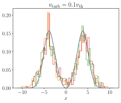
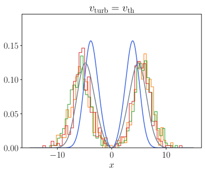
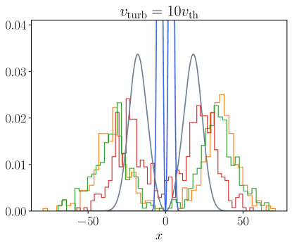
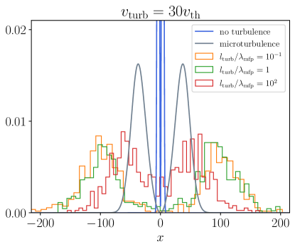
Figure 1: The spectrum of Ly$\alpha$ photons emerging from a turbulent sphere with the line center optical depth of $\tau_{0}=10^{5}$ and temperature of $T=10^{4}\>\textrm{K}$. For each fixed value of the turbulence velocity $v_{\textrm{turb}}$ [$v_{\textrm{turb}}=0.1v_{\textrm{th}}$ (top left), $v_{\textrm{turb}}=v_{\textrm{th}}$ (top right), $v_{\textrm{turb}}=10v_{\textrm{th}}$ (bottom left), $v_{\textrm{turb}}=30v_{\textrm{th}}$ (bottom right)] each subplot shows the histogram of the emergent spectrum for several values of the turbulence correlation length $l_{\textrm{turb}}$ [$l_{\textrm{turb}}=10^{-1}\lambda_{\textrm{mfp}}$ (orange), $l_{\textrm{turb}}=\lambda_{\textrm{mfp}}$ (green), $l_{\textrm{turb}}=10^{2}\lambda_{\textrm{mfp}}$ (red)] as well as the Neufeld analytical solution (Neufeld, 1990) for the cases with no turbulence (royalblue) and with microturbulence (slategray).

2 Model description

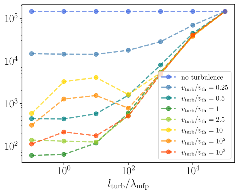
Figure 2: Top panel: The average number of scattering events $N_{\textrm{scat}}$ that a representative photon undergoes before it escapes the turbulent cloud of neutral hydrogen versus the turbulence correlation length $l_{\textrm{turb}}$ for different values of the turbulence velocity amplitude $v_{\textrm{turb}}$ [$v_{\textrm{turb}}=0.25v_{\textrm{th}}$ (steelblue), $v_{\textrm{turb}}=0.5v_{\textrm{th}}$ (teal), $v_{\textrm{turb}}=v_{\textrm{th}}$ (forestgreen), $v_{\textrm{turb}}=2.5v_{\textrm{th}}$ (yellowgreen), $v_{\textrm{turb}}=10v_{\textrm{th}}$ (gold), $v_{\textrm{turb}}=10^{2}v_{\textrm{th}}$ (darkorange), $v_{\textrm{turb}}=10^{3}v_{\textrm{th}}$ (orangered)] as well as for the case with no turbulence (royalblue). Bottom panel: The average number of scattering events $N_{\textrm{scat}}$ that a representative photon undergoes versus the turbulence velocity $v_{\textrm{turb}}$ for different values of the turbulence correlation length $l_{\textrm{turb}}$ [$l_{\textrm{turb}}=10^{-1}\lambda_{\textrm{mfp}}$ (teal), $l_{\textrm{turb}}=\lambda_{\textrm{mfp}}$ (forestgreen), $l_{\textrm{turb}}=10\lambda_{\textrm{mfp}}$ (yellowgreen), $l_{\textrm{turb}}=10^{2}\lambda_{\textrm{mfp}}$ (gold), $l_{\textrm{turb}}=10^{3}\lambda_{\textrm{mfp}}$ (darkorange), $l_{\textrm{turb}}=10^{4}\lambda_{\textrm{mfp}}$ (orangered)] as well as for the case with no turbulence (royalblue).

Our Monte Carlo radiative transfer code, except for the turbulence handling, largely follows the Monte Carlo procedure described in Dijkstra (2017) (see also Laursen 2010). Our goal is to have a macroscopic (bulk) velocity field $\mathbf{v}_{\textrm{turb}}$ that has an effective correlation length $l_{\textrm{turb}}$. There could be at least two ways to accomplish this. First approach is to divide the sphere into the cells of size $l_{\textrm{turb}}$ with each cell having its own $\mathbf{v}_{\textrm{turb}}$ drawn from the normal distribution and then launch photons through this fixed preassigned grid. However, such a procedure would be unnecessary memory and computationally heavy for our purposes, since we are interested in the averaged properties of the escaped radiation rather than the precise distribution inside the sphere. So instead we pursue the following approach. We draw a new random velocity $\mathbf{v}_{\textrm{turb}}$ from the normal distribution each time photon traveled a physical distance exceeding $l_{\textrm{turb}}$. Such division into "cells" is not preassigned but generated on the fly for each photon independently as it propagates. We note that some similar ideas were also used in Magnan (1976) and labeled as the effective cells approach.

First, we run our code without turbulence and make sure it agrees with known analytical solutions or previously studied numerical models. In particular we compared the solutions for static, expanding, and contracting uniform spherical cloud such as those studied in Zheng & Miralda-Escude (2002). We also considered three models of anisotropic hydrogen clouds, namely the density gradient, the velocity gradient, and the bipolar wind models, as described in Zheng & Wallace (2014). The code, its description, and the test results can be found in the GitHub repository Munirov & Kaurov (2022) (and in Appendix here).

Throughout the paper we use definitions of the variables and functions as those in Dijkstra (2017), unless stated otherwise explicitly. We assume that the readers are familiar with the basics of the Ly$\alpha$ transfer problem, otherwise it is recommended to consult Dijkstra (2017) (see also Laursen 2010). Specifically, we use the dimensionless photon frequency $x=\left(\nu-\nu_{\alpha}\right)/\Delta\nu_{\alpha}$, where $\Delta\nu_{\alpha}/\nu_{\alpha}=b/c$, $b$ is the Doppler broadening parameter, $c$ is the speed of light, and $\nu_{\alpha}=2.47\times 10^{15}\>\textrm{Hz}$ is the frequency at the Ly$\alpha$ line center. We use $\lambda_{\textrm{mfp}}$ to denote the mean free path of a photon at the line center $\lambda_{\textrm{mfp}}\equiv\lambda_{\textrm{mfp}}\left(x=0\right)$ in the hydrogen cloud without turbulence. We denote the optical depth from the center of the cloud to the edge for the line center photons without turbulence by $\tau_{0}$. We define the thermal velocity as $v_{\textrm{th}}=\sqrt{2k_{B}T/m_{p}}$, where $k_{B}$ is the Boltzmann constant, $m_{p}$ is the proton mass, and $T$ is the gas temperature in Kelvins. We use the following definition for the Voigt function $H(a,x)$:

$$H(a,x)=\frac{a}{\pi}\int_{-\infty}^{\infty}\frac{e^{-\xi^{2}}d\xi}{\left(\xi-x\right)^{2}+a^{2}},$$ (1)

where $a=4.7\times 10^{-4}$$(T/10^{4}\>\textrm{K})^{-1/2}$ is the Voigt parameter. In all our simulations of the turbulence we consider a uniform sphere of radius $R=1$ (so that all the distances are measured in the units of $R$, in particular the mean free path at the line center is $\lambda_{\textrm{mfp}}=\tau_{0}^{-1}$) with a point source at the center of the sphere; we include the recoil effect but ignore photon absorption due to dust; we consider Ly$\alpha$ system decoupled from a Hubble flow. The integration step is chosen to be a small enough fraction of $l_{\textrm{turb}}$, so that we always resolve a turbulent cell numerically.

In the next section we present and discuss the numerical solutions obtained using the Monte Carlo code described in this section.

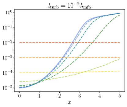
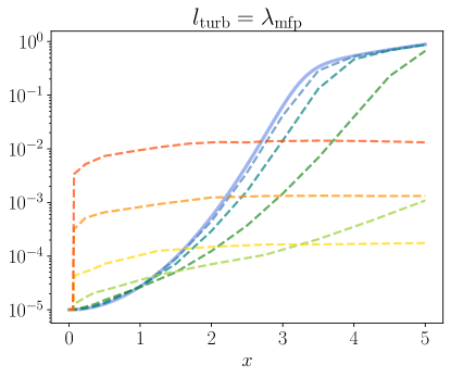
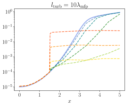
Figure 3: The numerically calculated effective mean free path versus the dimensionless frequency $x$. For each fixed value of the turbulence correlation length $l_{\textrm{turb}}$ [$l_{\textrm{turb}}=10^{-2}\lambda_{\textrm{mfp}}$ (top left), $l_{\textrm{turb}}=\lambda_{\textrm{mfp}}$ (top right), $l_{\textrm{turb}}=10\lambda_{\textrm{mfp}}$ (bottom left), $l_{\textrm{turb}}=10^{3}\lambda_{\textrm{mfp}}$ (bottom right)] the corresponding subplot shows the effective mean three path as a function of $x$ for several values of the turbulence velocity $v_{\textrm{turb}}$ [$v_{\textrm{turb}}=0.25v_{\textrm{th}}$ (steelblue), $v_{\textrm{turb}}=0.5v_{\textrm{th}}$ (teal), $v_{\textrm{turb}}=v_{\textrm{th}}$ (forestgreen), $v_{\textrm{turb}}=2.5v_{\textrm{th}}$ (yellowgreen), $v_{\textrm{turb}}=10v_{\textrm{th}}$ (gold), $v_{\textrm{turb}}=10^{2}v_{\textrm{th}}$ (darkorange), $v_{\textrm{turb}}=10^{3}v_{\textrm{th}}$ (orangered)] as well as for the case with no turbulence (royalblue).

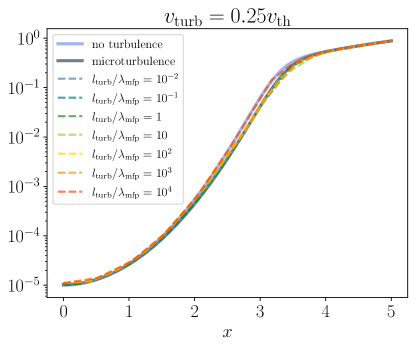
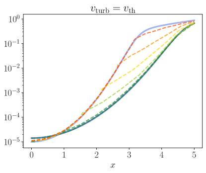
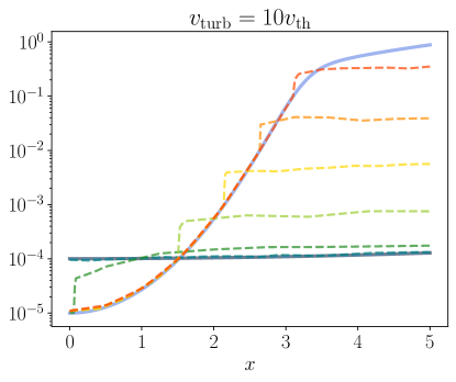
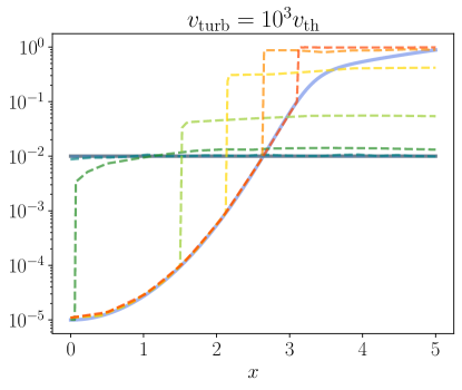
Figure 4: The numerically calculated effective mean free path versus the dimensionless frequency $x$. For each fixed value of the turbulence velocity $v_{\textrm{turb}}$ [$v_{\textrm{turb}}=0.25v_{\textrm{th}}$ (top left), $v_{\textrm{turb}}=v_{\textrm{th}}$ (top right), $v_{\textrm{turb}}=10v_{\textrm{th}}$ (bottom left), $v_{\textrm{turb}}=10^{3}v_{\textrm{th}}$ (bottom right)] the corresponding subplot shows the effective mean three path as a function of $x$ for the following values of the turbulence correlation length $l_{\textrm{turb}}$ [$l_{\textrm{turb}}=10^{-2}\lambda_{\textrm{mfp}}$ (steelblue), $l_{\textrm{turb}}=10^{-1}\lambda_{\textrm{mfp}}$ (teal), $l_{\textrm{turb}}=\lambda_{\textrm{mfp}}$ (forestgreen), $l_{\textrm{turb}}=10\lambda_{\textrm{mfp}}$ (yellowgreen), $l_{\textrm{turb}}=10^{2}\lambda_{\textrm{mfp}}$ (gold), $l_{\textrm{turb}}=10^{3}\lambda_{\textrm{mfp}}$ (darkorange), $l_{\textrm{turb}}=10^{4}\lambda_{\textrm{mfp}}$ (orangered)] as well as for the cases with no turbulence (royalblue) and with microturbulence (slategray).

3 Simulations results

Let us consider a uniform turbulent cloud of neutral hydrogen with the line center optical depth of $\tau_{0}=10^{5}$ and with the typical temperature of the neutral gas in the intergalactic medium of $T=10^{4}\>\textrm{K}$. This corresponds to the hydrogen column density of $n_{\textrm{HI}}\approx 1.7\times 10^{18}\>\textrm{c$\textrm{m}^{-2}$}$ and the Voigt parameter $a$ such that $a\tau_{0}\approx 47$.

We run the Monte Carlo simulations for several values of the turbulence correlation length $l_{\textrm{turb}}$ ranging from $l_{\textrm{turb}}=10^{-1}\lambda_{\textrm{mfp}}$ to $l_{\textrm{turb}}=10^{4}\lambda_{\textrm{mfp}}$ and several values of the turbulence velocity amplitude $v_{\textrm{turb}}$ ranging from $v_{\textrm{turb}}=0$ to $v_{\textrm{turb}}=10^{3}v_{\textrm{th}}$. We launch $10^{5}$ photons for each set of the parameters and when the photons leave the turbulent cloud we register their frequencies and the total number of scatterings they experienced.

The spectrum of the Ly$\alpha$ photons emerging from a spherical cloud of turbulent neutral hydrogen is shown in Fig. 1. For a fixed value of the turbulence velocity $v_{\textrm{turb}}$ ($v_{\textrm{turb}}/v_{\textrm{th}}=0.1,1,10,30$) each subplot shows the histogram of the emerging spectrum for three values of the turbulence correlation length $l_{\textrm{turb}}$ ($l_{\textrm{turb}}/\lambda_{\textrm{mfp}}=10^{-1},1,10^{2}$) as well as the Neufeld analytical solution (Neufeld, 1990) for the cases without turbulence and with microturbulence for the corresponding value of $v_{\textrm{turb}}$.

We can see from Fig. 1 that in the presence of turbulence the emergent spectrum is still double peaked but the peaks of the spectrum move further away from the line center. Due to the recoil effect, the spectrum has a slight asymmetry with more photons scattered into smaller frequencies, but for larger values of the turbulence velocity, this asymmetry diminishes. For $v_{\textrm{turb}}\lesssim v_{\textrm{th}}$, the emergent spectrum can be approximately described by the microturbulence model, while for $v_{\textrm{turb}}\gtrsim v_{\textrm{th}}$, the difference is substantial even for small correlation lengths of the turbulence ($l_{\textrm{turb}}=10^{-1}\lambda_{\textrm{mfp}}$).

The more surprising result is a significant reduction in the total number of scattering events $N_{\textrm{scat}}$ undergone by the Ly$\alpha$ photons before they escape the gas cloud. The top row of Fig. 2 shows the average number of scatterings that a Ly$\alpha$ photon experiences before it escapes as a function of the turbulence correlation length $l_{\textrm{turb}}$ for different values of the turbulence velocity amplitude $v_{\textrm{turb}}$, while the bottom row of Fig. 2 shows the average number of scatterings $N_{\textrm{scat}}$ versus the turbulence velocity $v_{\textrm{turb}}$ for different values of the turbulence correlation length $l_{\textrm{turb}}$. In addition, the number of scatterings events $N_{\textrm{scat}}$ for the case without turbulence is shown in both subplots.

We can see from Fig. 2 that without turbulence the average number of scattering events $N_{\textrm{scat}}$ is at the order of the optical depth $\tau_{0}=10^{5}$, which agrees with the well known result (Adams, 1972; Harrington, 1973; Dijkstra, 2017) that in the absence of turbulence the number of scatterings for optically thick case is given by $N_{\textrm{scat}}=C\tau_{0}$, where $C$ is a numerical constant of order one. We can also see that for $v_{\textrm{turb}}/v_{\textrm{th}}\rightarrow 0$ and $l_{\textrm{turb}}/\lambda_{\textrm{mfp}}\rightarrow\infty$ the average number of scatterings is also approaching $\tau_{0}=10^{5}$, as expected because these cases converge to the absence of turbulence. Overall, the number of scatterings depends on $l_{\textrm{turb}}$ and $v_{\textrm{turb}}$ in a complicated manner, but, similarly to the case of expanding/contracting gas (Bonilha et al., 1979), there is a decrease in the number of scattering events for all parameters of turbulence.

Turbulence influences the scattering process in two ways. First, for a given optical depth generated from an exponential distribution $P\left(\tau\right)=e^{-\tau}$ the effective mean free path is changed because the photon frequency in the local frame of the gas depends on the turbulent bulk motion of the medium: $x^{\prime}=x-\mathbf{v}_{\textrm{bulk}}\left(\mathbf{r}^{\prime}\right)\cdot\mathbf{k}/v_{\textrm{th}}$. Second, once the scattering cell is determined, the photon besides experiencing the usual frequency redistribution in the gas frame, gets an additional Lorentz transformed frequency shift $\mathbf{v}_{\textrm{bulk}}\cdot\left(\mathbf{k}_{\textrm{out}}-\mathbf{k}_{\textrm{in}}\right)/v_{\textrm{th}}$ in the laboratory frame. This leads to an additional random jump in frequency space on the order of $\left|\triangle x\right|\approx v_{\textrm{turb}}/v_{\textrm{th}}$ and results in faster transition from the core to the wings of the Voigt profile. Since scattering in the cell is always local by definition, once the scattering cell is determined the turbulence correlation length does not matter. Thus, even if the correlation length is very small, turbulence can still influence the photon propagation through the above mentioned random frequency jumps.

To better understand how the presence of turbulence with a finite correlation length changes the mean free path for propagating photons, we computed the effective mean free path in the following way: for an optical depth drawn from a Poisson distribution with $\tau=1$ a test photon of frequency $x$ is launched a sufficient number of times (hundreds was enough to achieve stable results) with fixed values of $v_{\textrm{turb}}$ and $l_{\textrm{turb}}$ and the effective mean free path is then calculated as an average of these launches.

Figs. 3 and 4 show the effective mean free path versus the dimensionless frequency $x$. In Fig. 3, for each fixed value of the turbulence correlation length $l_{\textrm{turb}}$ ($l_{\textrm{turb}}/\lambda_{\textrm{mfp}}=10^{-2},1,10,10^{3}$) we plot the effective mean free path as a function of $x$ for several values of the turbulence velocity $v_{\textrm{turb}}$ ($v_{\textrm{turb}}/v_{\textrm{th}}=0.25,0.5,1,2.5,10,10^{2},10^{3}$) and for the case with no turbulence. In Fig. 4, for each fixed value of the turbulence velocity $v_{\textrm{turb}}$ ($v_{\textrm{turb}}/v_{\textrm{th}}=0.25,1,10,10^{3}$) we plot the effective mean free path as a function of $x$ for several values of the turbulence correlation length $l_{\textrm{turb}}$ ($l_{\textrm{turb}}/\lambda_{\textrm{mfp}}=10^{-2},10^{-1},1,10,10^{2},10^{3},10^{4}$) as well as the mean free paths in the absence of turbulence and with microturbulence for the corresponding value of $v_{\textrm{turb}}$. In the absence of turbulence, one gets the usual mean free path determined by the inverse of the Voigt profile: $\lambda_{\textrm{mfp}}\left(x\right)=1/\tau_{0}H\left(a,x\right)$, while for microturbulence one gets a properly scaled inverse of the Voigt profile:

$$\lambda_{\textrm{mfp}}\left(x\right)=\frac{\sqrt{1+v_{\textrm{turb}}^{2}/v_{\textrm{th}}^{2}}}{\tau_{0}H\left(\frac{a}{\sqrt{1+v_{\textrm{turb}}^{2}/v_{\textrm{th}}^{2}}},\frac{x}{\sqrt{1+v_{\textrm{turb}}^{2}/v_{\textrm{th}}^{2}}}\right)}.$$ (2)

We see from Figs. 3 and 4 that for $l_{\textrm{turb}}\ll\lambda_{\textrm{mfp}}$ ($l_{\textrm{turb}}/\lambda_{\textrm{mfp}}=10^{-2},10^{-1}$), the effective mean free path indeed matches the microturbulence curve for all values of the turbulence velocity. On the other hand, for large values of the turbulence correlation length $l_{\textrm{turb}}\gtrsim\lambda_{\textrm{mfp}}$, the effective mean free path follows the mean free path $\lambda_{\textrm{mfp}}\left(x\right)=1/\tau_{0}H\left(a,x\right)$ in the absence of turbulence up until some threshold value $x_{l}$, where the effective mean free path experiences jump and changes its dependence. The value of the threshold is essentially independent of the turbulence velocity amplitude $v_{\textrm{turb}}$ and depends mainly on the turbulence correlation length $l_{\textrm{turb}}$, and is approximately determined by the condition $\lambda_{\textrm{mfp}}\left(x_{l}\right)=l_{\textrm{turb}}$ or, equivalently, $H\left(a,x_{l}\right)=l_{\textrm{turb}}^{-1}$.

Going back to Fig. 2, we see that for $v_{\textrm{turb}}\lesssim v_{\textrm{th}}$, the number of scatterings $N_{\textrm{scat}}$ decreases as the turbulence velocity amplitude $v_{\textrm{turb}}$ increases. It can be understood in the following way. While the effective mean free path is not changed dramatically for $v_{\textrm{turb}}\lesssim v_{\textrm{th}}$ (see Fig. 4), turbulence still brings random jumps in frequency space with the characteristic size $\left|\triangle x\right|\approx v_{\textrm{turb}}/v_{\textrm{th}}\lesssim 1$; these random jumps allow photons to move from the core to the wings in fewer scatterings (the core-wing boundary for our parameters is at $\left|x\right|\approx 3.26$). The bigger those jumps, the faster the photons jump from the core to the wings, which is why we see a decrease in the number of scatterings for $v_{\textrm{turb}}\lesssim v_{\textrm{th}}$ as $v_{\textrm{turb}}$ approaches $v_{\textrm{th}}$. For larger values of the turbulence velocity amplitude $v_{\textrm{turb}}\gtrsim v_{\textrm{th}}$, we see that the number of scatterings $N_{\textrm{scat}}$ generally exhibits a non-monotonic dependence on $v_{\textrm{turb}}$. Here we have a competition between the change in the effective mean free path and large, often exceeding the width of the core region, random frequency jumps on the order of $\left|\triangle x\right|\approx v_{\textrm{turb}}/v_{\textrm{th}}\gtrsim 1$.

We also see from Fig. 2 that the number of scatterings $N_{\textrm{scat}}$ generally speaking decreases as the turbulence correlation length $l_{\textrm{turb}}$ decreases. At small but finite values of the turbulence correlation length $l_{\textrm{turb}}$ the random frequency jumps are largely localized in space and happen often enough to drive Ly$\alpha$ photons to the wings, which allows them to escape in fewer scatterings. For sufficiently large values of $l_{\textrm{turb}}$, the number of scatterings inside a region of size $l_{\textrm{turb}}$ is approximately given by $\tau_{\textrm{eff}}=l_{\textrm{turb}}/\lambda_{\textrm{mfp}}$, if in addition $v_{\textrm{turb}}\gtrsim v_{\textrm{th}}$, then once the photons random walked out of the region of size $l_{\textrm{turb}}$ it will likely escape, so that the total number of scatterings is approximately $N_{\textrm{scat}}\approx\tau_{\textrm{eff}}=l_{\textrm{turb}}/\lambda_{\textrm{mfp}}$. Indeed, we see from Fig. 2 that for $v_{\textrm{turb}}\gtrsim v_{\textrm{th}}$ and for large values of the turbulence correlation length between approximately $l_{\textrm{turb}}/\lambda_{\textrm{mfp}}=10$ and $l_{\textrm{turb}}/\lambda_{\textrm{mfp}}=10^{5}$ the number of scatterings scales as $N_{\textrm{scat}}\approx 4l_{\textrm{turb}}/\lambda_{\textrm{mfp}}$.

We conclude by pointing out that the exact dependence of the number of scatterings $N_{\textrm{scat}}$ on $l_{\textrm{turb}}$ and $v_{\textrm{turb}}$ and its sensitivity to changes in these parameters is complicated and also depends on the characteristics, such as density and temperature, of the HI regions though which Ly$\alpha$ photons propagate. However, overall, the presence of turbulence makes it easier for Ly$\alpha$ photons to be scattered into the wings, facilitating their escape and reducing the number of scattering events they experience.

4 Conclusion

In this paper we focused on the qualitative analysis of the turbulence effect on the Ly$\alpha$ transfer. We adopted a Monte Carlo approach and considered a simple geometry with turbulence represented as spatial domains of given size with randomly directed velocities.

We performed numerical simulations and discovered that the presence of turbulence not only alters the emergent spectrum, but turbulence with small but finite correlation length can significantly, by orders of magnitude, reduce the number of scatterings required for the Ly$\alpha$ photons to escape the cloud of neutral hydrogen. The reduction in the average number of scattering events can, for example, lead to a decrease in the effectiveness of the Wouthuysen–Field coupling (Wouthuysen, 1952; Field, 1958, 1959) of the spin temperature to Ly$\alpha$ radiation or affect the polarization of the scattered photons, since both are influenced by the number of resonant scattering events (Roy et al., 2009; Dijkstra & Loeb, 2008; Ahn & Lee, 2015; Seon & Kim, 2020; Seon et al., 2022).

We conclude that modeling turbulence as an effective temperature (microturbulence) has a limited area of applicability. On one hand, our study confirms the importance of coupling radiative transfer codes with detailed hydrodynamic simulations (Smith et al., 2020). On the other hand, our approach provides a simplified alternative when the use of full hydrodynamic simulations is limited by computational resources or by the availability of reliable physical inputs. Thus, our model is especially useful in the regions where the scale of the turbulence is too large to be described as microturbulence but at the same time is too small to be realistically resolved by full hydrodynamic simulations.

Finally, we point out that the propagation of Ly$\alpha$ photons can have an effect on the macroscopic motion of the neutral gas itself. Indeed, Ly$\alpha$ photons can transfer momentum between layers of the moving gas equilibrating their relative motion through radiative viscosity similar to the case of radiative viscosity due to Thomson scattering (Loeb & Laor, 1992), with the crucial difference being that unlike Thomson scattering, the mean free path of the Ly$\alpha$ photons is not constant but sensitively, by orders of magnitude, depends on the photon wavelength.

Data Availability

The code and some data underlying this article are available in the GitHub repository Munirov & Kaurov (2022) at https://github.com/dimmun/LyAMC. The additional data underlying this article will be shared on reasonable request to the corresponding author.

Appendix A Acceptance rate for get_upar

To pick a random parallel velocity for scattering atom we use the rejection method. In this method we use parameter $u_{0}$ that determines acceptance rate and thus can accelerate computations if chosen wisely. Here is the comparison for the acceptance rate for the choice of $u_{0}$ used in our paper with (Semelin, B. et al., 2007) and (Laursen et al., 2009; Laursen, 2010)

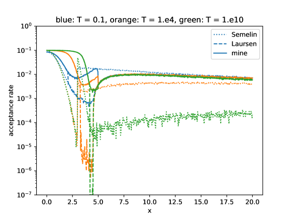
Figure 5: The acceptance rate for the choice of $u_{0}$ used in our paper with (Semelin, B. et al., 2007) and (Laursen et al., 2009; Laursen, 2010) for three different values of $T$ and fixed $\tau_{0}$ (consequently for three different values of parameter $a\tau_{0}$).

Appendix B Static cloud

The numerical solution for the case of static uniform cloud with a source in the center of a uniform sphere of static gas cloud emitting photons at line center with analytical results.

Figure 6: The emergent spectrum from a static uniform sphere for temperature $T=10^{4}\>\textrm{K}$ and two optical depths $\tau_{0}=10^{5}$ and $\tau_{0}=10^{6}$. The figure also shows the analytical solutions from Neufeld (Neufeld, 1990) using $\eta a\tau_{0}$ with $\eta=0.71$ (dashed line) and $\eta=1$ (dotted line) and from Dijkstra (Dijkstra et al., 2006a) (solid line).

Appendix C Expanding/contracting clouds

The numerical solution for the case of expanding and contracting uniform cloud with a source in the center of a uniform sphere of neutral hydrogen cloud emitting photons at line center. See Ref. Zheng & Miralda-Escude (2002).

Figure 7: The emergent spectrum from expanding ($v=200\>\textrm{km}/\textrm{s}$) and contracting ($v=-200\>\textrm{km}/\textrm{s}$) uniform spheres for optical depth $\tau_{0}=10^{7}$.

Appendix D Density gradient model

The density gradient model of Zheng & Wallace (2014). See Figs. 1 and 3 from Zheng & Wallace (2014).

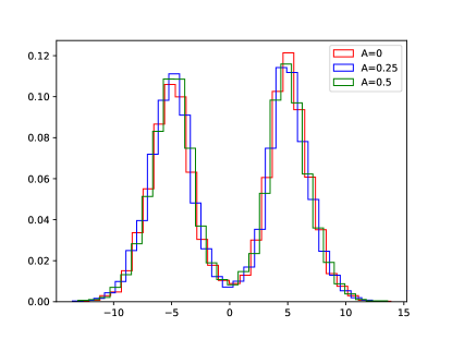
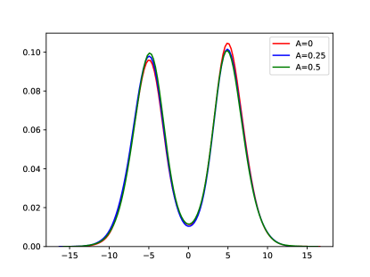
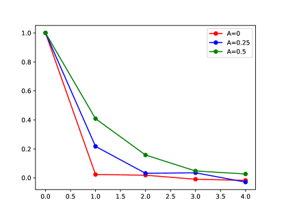
Figure 8: Results for the density gradient model (see Zheng & Wallace 2014).

Appendix E Velocity gradient model

The velocity gradient model of Zheng & Wallace (2014). See Figs. 5 and 7 from Zheng & Wallace (2014). There is some disagreement but the corresponding graph in Zheng & Wallace (2014) was actually computed for the parameters different from those reported in Zheng & Wallace (2014) [private communication].

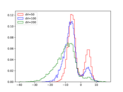
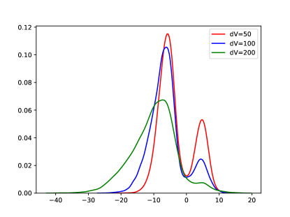
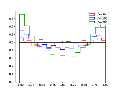
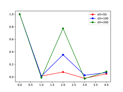
Figure 9: Results for the velocity gradient model (see Zheng & Wallace 2014).

Appendix F Bipolar wind model

The bipolar wind model of Zheng & Wallace (2014). See Fig. 9 from Zheng & Wallace (2014).

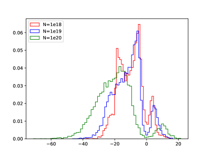
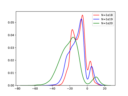
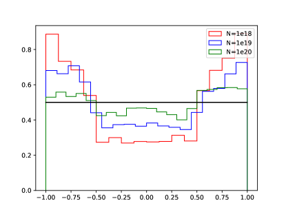
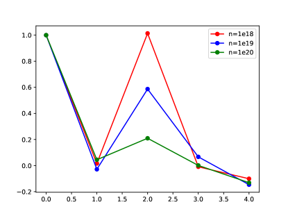
Figure 10: Results for the bipolar wind model (see Zheng & Wallace 2014).

Appendix G The number of scatterings $N_{\textrm{scat}}$ for $\tau_{0}=10^{5}$, $T=1\>\textrm{K}$, $a\tau_{0}\approx 4.7\times 10^{3}$

The number of scatterings $N_{\textrm{scat}}$ for $\tau_{0}=10^{5}$, $T=1\>\textrm{K}$, $a\tau_{0}\approx 4.7\times 10^{3}$.

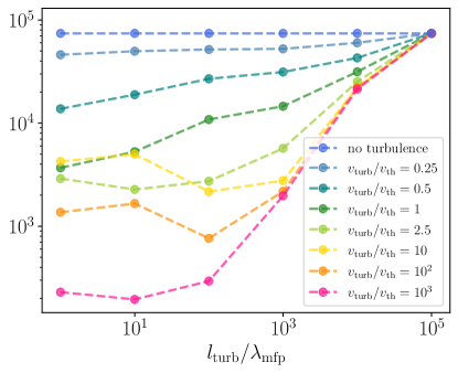
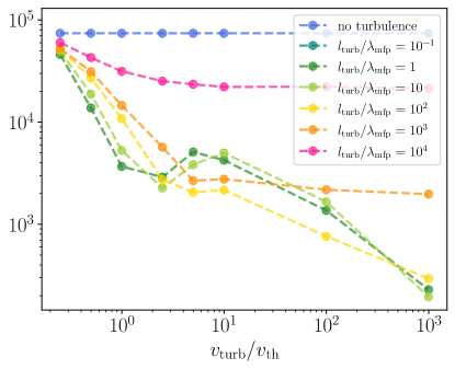
Figure 11: Left panel: The average number of scattering events $N_{\textrm{scat}}$ that a representative photon undergoes before it escapes the turbulent cloud of neutral hydrogen versus the turbulence correlation length $l_{\textrm{turb}}$ for different values of the turbulence velocity amplitude $v_{\textrm{turb}}$. Right panel: The average number of scattering events $N_{\textrm{scat}}$ that a representative photon undergoes versus the turbulence velocity $v_{\textrm{turb}}$ for different values of the turbulence correlation length $l_{\textrm{turb}}$. The temperature is $T=1\>\textrm{K}$ and the optical depth is $\tau_{0}=10^{5}$, which corresponds to a strongly optically thick case with the Voigt parameter $a$ such that $a\tau_{0}\approx 4.7\times 10^{3}$.

Appendix H The effective mean free path for $\tau_{0}=10^{5}$, $T=1\>\textrm{K}$, $a\tau_{0}\approx 4.7\times 10^{3}$

The effective mean free path for $\tau_{0}=10^{5}$, $T=1\>\textrm{K}$, $a\tau_{0}\approx 4.7\times 10^{3}$.

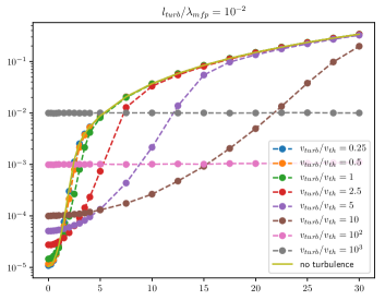
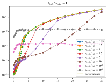
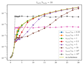
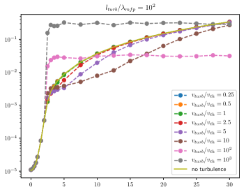
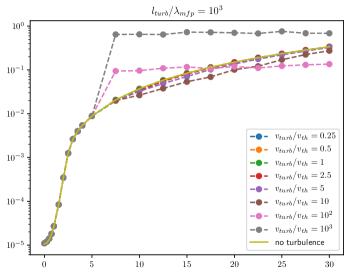
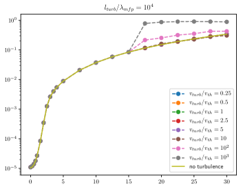
Figure 12: The numerically calculated effective mean free path versus the dimensionless frequency $x$ for $\tau_{0}=10^{5}$, $T=1\>\textrm{K}$, $a\tau_{0}\approx 4.7\times 10^{3}$. The effective mean free path versus dimensionless frequency $x$. For each of the fixed value of the turbulence correlation length $l_{turb}/\lambda_{mfp}=10^{-2},10^{-1},1,10,10^{2},10^{3},10^{4}$ the corresponding subgraph shows the effective mean three path as a function of $x$ for the following values of the turbulent velocity: $v_{turb}/v_{th}=0.25,0.5,1,2.5,5,10,10^{2}$, as well as for the case with no turbulence. $T=1\>\textrm{K}$. The parameters are $\tau_{0}=10^{5}$, $T=1\>\textrm{K}$, $a\tau_{0}\approx 4.7\times 10^{3}$.

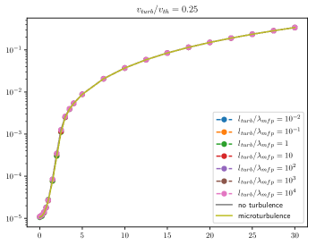
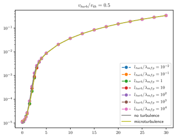
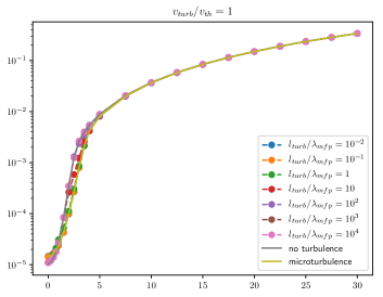
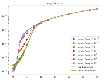
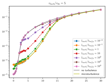
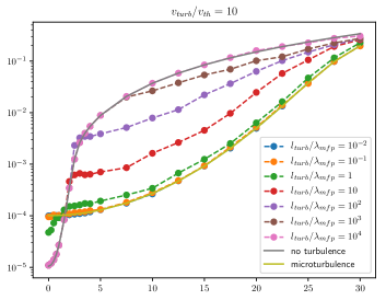
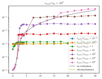
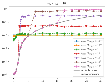
Figure 13: The numerically calculated effective mean free path versus the dimensionless frequency $x$ for $\tau_{0}=10^{5}$, $T=1\>\textrm{K}$, $a\tau_{0}\approx 4.7\times 10^{3}$. The effective mean free path versus dimensionless frequency $x$. For each of the fixed value of the turbulent velocity ($v_{turb}/v_{th}=0.25,0.5,1,2.5,5,10,10^{2}$) the corresponding subgraph shows the effective mean three path as a function of $x$ for the following values of the turbulence correlation length ($l_{turb}/\lambda_{mfp}=10^{-1},1,10,10^{2},10^{3},10^{4}$) as well as for the cases with no turbulence and with microturbulence. The parameters are $\tau_{0}=10^{5}$, $T=1\>\textrm{K}$, $a\tau_{0}\approx 4.7\times 10^{3}$.

References

- Adams (1972) Adams T. F., 1972, ApJ, 174, 439
- Ahn & Lee (2015) Ahn S.-H., Lee H.-W., 2015, JKAS, 48, 195
- Behnel et al. (2011) Behnel S., Bradshaw R., Citro C., Dalcin L., Seljebotn D. S., Smith K., 2011, CSE, 13, 31
- Behrens et al. (2019) Behrens C., Pallottini A., Ferrara A., Gallerani S., Vallini L., 2019, MNRAS, 486, 2197
- Ben Jaffel et al. (1993) Ben Jaffel L., Clarke J. T., Prangé R., Gladstone G. R., Vidal-Madjar A., 1993, GeoRL, 20, 747
- Bonilha et al. (1979) Bonilha J. R. M., Ferch R., Salpeter E. E., Slater G., Noerdlinger P. D., 1979, ApJ, 233, 649
- Burkhart (2021) Burkhart B., 2021, Publ. Astron. Soc. Pac., 133, 102001
- Dijkstra (2014) Dijkstra M., 2014, PASA, 31, e040
- Dijkstra (2017) Dijkstra M., 2017, Saas-Fee Lecture Notes: Physics of Lyman Alpha Radiative Transfer (arXiv:1704.03416)
- Dijkstra & Loeb (2008) Dijkstra M., Loeb A., 2008, MNRAS, 386, 492
- Dijkstra et al. (2006a) Dijkstra M., Haiman Z., Spaans M., 2006a, ApJ, 649, 14
- Dijkstra et al. (2006b) Dijkstra M., Haiman Z., Spaans M., 2006b, ApJ, 649, 37
- Eastman & MacAlpine (1985) Eastman R. G., MacAlpine G. M., 1985, ApJ, 299, 785
- Erb et al. (2018) Erb D. K., Steidel C. C., Chen Y., 2018, ApJ, 862, L10
- Field (1958) Field G. B., 1958, Proc. IRE, 46, 240
- Field (1959) Field G. B., 1959, ApJ, 129, 551
- Harrington (1973) Harrington J. P., 1973, MNRAS, 162, 43
- Hayes (2015) Hayes M., 2015, PASA, 32, e027
- Lam et al. (2015) Lam S. K., Pitrou A., Seibert S., 2015, in Proceedings of the Second Workshop on the LLVM Compiler Infrastructure in HPC. LLVM ’15. Association for Computing Machinery, New York, NY, USA, doi:10.1145/2833157.2833162
- Laursen (2010) Laursen P., 2010, PhD thesis, University of Copenhagen, https://arxiv.org/abs/1012.3175
- Laursen et al. (2009) Laursen P., Razoumov A. O., Sommer-Larsen J., 2009, ApJ, 696, 853
- Loeb & Laor (1992) Loeb A., Laor A., 1992, ApJ, 384, 115
- Loeb & Rybicki (1999) Loeb A., Rybicki G. B., 1999, ApJ, 524, 527
- Magnan (1976) Magnan C., 1976, JQSRT, 16, 281
- McQuinn et al. (2007) McQuinn M., Hernquist L., Zaldarriaga M., Dutta S., 2007, MNRAS, 381, 75
- Munirov & Kaurov (2022) Munirov V. R., Kaurov A. A., 2022, https://github.com/dimmun/LyAMC
- Neufeld (1990) Neufeld D. A., 1990, ApJ, 350, 216
- Ouchi et al. (2020) Ouchi M., Ono Y., Shibuya T., 2020, ARA&A, 58, 617
- Puschnig, J. et al. (2020) Puschnig, J. et al., 2020, A&A, 644, A10
- Roy et al. (2009) Roy I., Xu W., Qiu J.-M., Shu C.-W., Fang L.-Z., 2009, ApJ, 694, 1121
- Semelin, B. et al. (2007) Semelin, B. Combes, F. Baek, S. 2007, A&A, 474, 365
- Seon & Kim (2020) Seon K.-I., Kim C.-G., 2020, ApJS, 250, 9
- Seon et al. (2022) Seon K.-I., Song H., Chang S.-J., 2022, ApJS, 259, 3
- Smith et al. (2018) Smith A., Tsang B. T.-H., Bromm V., Milosavljević M., 2018, MNRAS, 479, 2065
- Smith et al. (2020) Smith A., Kannan R., Tsang B. T.-H., Vogelsberger M., Pakmor R., 2020, ApJ, 905, 27
- Smith et al. (2022) Smith A., et al., 2022, MNRAS, 517, 1
- Van Rossum & Drake (2009) Van Rossum G., Drake F. L., 2009, Python 3 Reference Manual. CreateSpace, Scotts Valley, CA
- Wolfe et al. (2005) Wolfe A. M., Gawiser E., Prochaska J. X., 2005, ARA&A, 43, 861
- Wouthuysen (1952) Wouthuysen S. A., 1952, AJ, 57, 31
- Yuen et al. (2022) Yuen K. H., Ho K. W., Law C. Y., Chen A., Lazarian A., 2022, Turbulent universal galactic Kolmogorov velocity cascade over 6 decades (arXiv:2204.13760)
- Zheng & Miralda-Escude (2002) Zheng Z., Miralda-Escude J., 2002, ApJ, 578, 33
- Zheng & Wallace (2014) Zheng Z., Wallace J., 2014, ApJ, 794, 116