$H_{\infty}$-optimal control of coupled ODE-PDE systems using PIE framework and LPIs

Abstract

In this paper, we present a dual formulation for Lyapunov’s stability test and Bounded-real Lemma for Partial Integral Equations (PIEs). Then, we use this formulation to solve the $H_{\infty}$-optimal controller synthesis problem for ODE-PDEs that can be converted to a PIE. First, we provide a general dual criterion for the Lyapunov stability and the Bounded-real Lemma for PIEs using quadratic Lyapunov functionals. Then, we use a class of operators called Partial Integral (PI) operators to parametrize the said Lyapunov functional and express the dual criterion as an operator-valued convex optimization problem with sign-definite constraints on PI operators — called Linear PI Inequalities (LPIs). Consequently, the optimal controller synthesis problem for PIEs, and thus, for PDEs, is formulated as LPIs. Finally, the LPI optimization problems are solved using a computational toolbox called PIETOOLS and tested on various examples to demonstrate the utility of the proposed method.

I Introduction

Models of Ordinary Differential equations (ODEs) coupled with Partial Differential Equations (PDEs) are used to describe many phenomena such as spatially-distributed chemical/nuclear reactions (e.g., chemical reactors and tokamaks), the motion of soft-robots (for e.g., octopus-inspired robots), etc. Typically, the coupling with the ODE arises due to the inclusion of a lumped state (for example, wall temperature in chemical reactors or central robot body in the case of soft-robots), and the coupling can be through the boundary or the dynamics. Various methods have been developed to design controllers for systems modeled as coupled ODE-PDEs, such as, the method of Backstepping (See e.g. [11]), frequency-domain methods [1], and discretization-based methods (See e.g. [8, 9, 3]). However, these approaches have limitations (as will be discussed below) and this paper aims to propose a new computational approach for controller design that can overcome those limitations.

In Backstepping methods, control input acts through the boundary, and as such, these techniques, in most cases, provide an explicit controller with provable stability properties. However, the controllers so obtained are not optimal in any sense. In the latter two cases (frequency-domain and discretization-based methods), $H_{\infty}$-optimal controllers are designed for an ODE approximation of the PDE system. Unlike the backstepping method, these controllers typically do not have provable stability (or input-output) properties when used on the original PDE, i.e., the $H_{\infty}$-norm of the ODE-PDE system is not the same as the $H_{\infty}$-norm of the ODE approximation, and indeed, the resulting closed-loop system can become unstable. Furthermore, frequency-domain approaches (for example, [20, 12]) design an optimal controller using the transfer function of the ODE-PDE system. However, the concept of a transfer function is not extendable to systems with multiple inputs/outputs and, thus, may require decoupling of the equations in the ODE-PDE before the application of analysis or control design techniques.

Thus, this paper aims to propose computational methods that can be used to solve the $H_{\infty}$-optimal control problem for the coupled ODE-PDE systems where the control input can act through the boundary, in-domain, or both. The methods proposed here are similar to Linear Matrix Inequality (LMI) methods used to design a controller for ODEs. To use LMIs for controller design, ODEs are first written in a standard form such as $9$-matrix representation [2] and then the dual formulation of the Lyapunov stability test is used to find the controller. A standard representation is necessary in a computational tool to minimize the number of ad-hoc steps needed to define and solve an optimization problem, whereas the dual stability test is needed since the controller synthesis problem is a non-convex optimization problem as shown below.

The fundamental issue in controller synthesis for both finite-dimensional and infinite-dimensional systems is the bilinear constraint. In simple terms, for either a finite or infinite-dimensional system of the form

$$\dot{x}(t)=\mathcal{A}x(t)+\mathcal{B}u(t),\quad x(t)\in X$$

finding a stabilizing control $u(t)=\mathcal{K}x(t)$ and a corresponding Lyapunov functional $V(t)=\left\langle{x(t)},{\mathcal{P}x(t)}\right\rangle_{X}$ with negative time-derivative leads to a bilinear problem in variables $\mathcal{K}$ and $\mathcal{P}$ of the form $(\mathcal{A}+\mathcal{BK})^{*}\mathcal{P}+\mathcal{P}(\mathcal{A}+\mathcal{BK})\leq 0$.

In case of linear ODEs, the linear operators $\mathcal{P},\mathcal{K},\mathcal{A}$ and $\mathcal{B}$ are just matrices $P$, $K$, $A$ and $B$. In absence of a controller, the Lyapunov stability test (referred to as primal stability test) can be written as an LMI in positive matrix variable $P>0$ such that $A^{T}P+PA\leq 0$. Since the eigenvalues of $A$ and $A^{T}$ are the same, there is an equivalent dual Lyapunov inequality of the form $AP+PA^{T}\leq 0$ (referred to as dual stability test). Then the test for the existence of a stabilizing controller $K$ and a Lyapunov functional $P$ which proves the stability of the closed-loop system can now be written as: find $P>0$ such that $(A+BK)P+P(A+BK)^{T}\leq 0$. The key difference, however, is the bilinearity can now be eliminated by introducing a new variable $Z=KP$ which leads to the LMI constraint $AP+BZ+(AP+BZ)^{T}\leq 0$.

Linear PDEs (and, by extension, ODE-PDEs), however, neither have any standard representation nor does there exist a dual formulation of Bounded-real Lemma for PDEs. The first step, then, is to present a parametric form for the class of ODE-PDEs (a standard representation) for which the optimal control problem is solved in this paper. While the representation for linear PDEs introduced in [15] does provide a standard representation for PDEs with $2^{nd}$-order spatial derivatives, coupled ODE-PDEs with inputs and outputs cannot be represented in that form. Thus, we first extend the representation to include parameters related to the ODE, the inputs, and the outputs.

The second step is finding a dual stability test for PDEs. For infinite-dimensional systems, Theorem $5.1.3$ of [4] is analogous to the primal stability test for ODEs, however, a dual version for the stability of PDEs does not exist. The primal stability test for PDEs is similar to that of ODEs in the sense that matrices in the constraints of the primal stability test for ODE are replaced by linear operators for infinite-dimensional systems, i.e. a test for the existence of a positive operator $\mathcal{P}>0$ that satisfies the operator-valued constraint $\mathcal{A}^{*}\mathcal{P}+\mathcal{PA}\leq 0$. However, there does not exist a dual form of the stability test for infinite-dimensional systems. In [13], a dual Lyapunov criterion for stability in infinite-dimensional systems was presented. However, the result was restricted to infinite-dimensional systems of the form

$$\dot{\mathbf{x}}(t)=\mathcal{A}\mathbf{x}(t)+\mathcal{B}u(t)$$

and included constraints on the image of the operator $\mathcal{P}$ of the form $\mathcal{P}(X)=X$ where $X=D(\mathcal{A})$ is the domain of the infinitesimal generator $\mathcal{A}$. Furthermore, because $\mathcal{A}$ for PDEs is a differential operator, this approach provides no way of enforcing the negativity of the dual stability condition. These difficulties in analysis and controller synthesis for PDE systems led to the development of the Partial Integral Equation (PIE) formulation of the problem - wherein both system parameters $\mathcal{A},\mathcal{B},\mathcal{C},\mathcal{D},\mathcal{T}$ and the Lyapunov parameter $\mathcal{P}$ lie in the algebra of bounded linear Partial Integral (PI) operators.

I-A Benefits of PIE representation: LPI tests for PIEs

PIEs have a $12$ PI representation, analogous to $9$-matrix representation of linear ODEs, as shown in Eq. (I-A).

$$\mathcal{T}\dot{\mathbf{x}}(t)+\mathcal{T}_{w}\dot{w}(t)+\mathcal{T}_{u}\dot{u}(t) =\mathcal{A}\mathbf{x}(t)+\mathcal{B}_{1}w(t)+\mathcal{B}_{2}u(t)$$

$$z(t) =\mathcal{C}_{1}\mathbf{x}(t)+\mathcal{D}_{11}w(t)+\mathcal{D}_{12}u(t)$$

$$y(t) =\mathcal{C}_{2}\mathbf{x}(t)+\mathcal{D}_{21}w(t)+\mathcal{D}_{22}u(t)$$ (1)

where $\mathbf{x}(t)\in\mathbb{R}^{m}\times L_{2}^{n}[a,b]$ is Fréchet differentiable, $w(t)\in\mathbb{R}^{p}$, $u(t)\in\mathbb{R}^{q}$ are differentiable, and the operators $\mathcal{T}$, $\mathcal{T}_{w}$, $\mathcal{T}_{u}$, $\mathcal{A}$, $\mathcal{B}_{i}$, $\mathcal{C}_{i}$, $\mathcal{D}_{ij}$ are 4-PI operators as defined in Section IV. Similar to the use of LMIs for ODEs, there exist Linear PI Inequalities (LPIs) to test for stability [15], find $H_{\infty}$-gain [19] and design $H_{\infty}$-optimal estimator [5] for PIEs. Furthermore, just like LMIs, LPIs are convex solvable inequalities and are solved using the toolbox PIETOOLS [18].

For example, if $\mathcal{T}_{w}=\mathcal{T}_{u}=0$ and inputs are zero, then the LPI for the stability of the PIE is given by

$$\mathcal{P}\succ 0$$

$$\mathcal{A}^{*}\mathcal{P}\mathcal{T}+\mathcal{T}^{*}\mathcal{P}\mathcal{A}\prec 0.$$ (2)

Thus, if an ODE-PDE can be rewritten in the form Eq. (I-A), then the stability of ODE-PDE can be proved using the LPI (I-A).

Since it has been shown that almost any ODE-PDE system in a single spatial dimension has an equivalent PIE system representation [17] (see Sec. III) which preserves both stability and I/O properties, we can use LPI tests to indirectly prove properties of the ODE-PDE system. More specifically, these methods apply for linear ODE-PDE systems in $1$ spatial variable with a very general set of boundary conditions including Dirichlet, Neumann, Robin, Sturm-Lioville etc. The resulting LPIs are solved numerically using PIETOOLS, an open-source MATLAB toolbox to handle PI variables and set up PI operator-valued optimization problems.

I-B Benefits of PIE representation: Duality in PIEs

In this paper, we consider the problem of $H_{\infty}$-optimal state-feedback controller synthesis for Partial Integral Equation (PIE) systems of the form

$$\mathcal{T}\dot{\mathbf{x}}(t) =\mathcal{A}\mathbf{x}(t)+\mathcal{B}u(t),\quad\mathbf{x}(0)=\mathbf{x}_{0}\in\mathbb{R}^{m}\times L_{2}^{n}$$

$$z(t) =\mathcal{C}\mathbf{x}(t)+\mathcal{D}u(t)$$ (3)

where $\mathcal{T},\mathcal{A},\mathcal{B},\mathcal{C},\mathcal{D}$ are PI operators and $u(t)\in\mathbb{R}^{p}$. The dual (or adjoint) PIE system is then defined to be

$$\mathcal{T}^{*}\dot{\bar{\mathbf{x}}}(t) =\mathcal{A}^{*}\bar{\mathbf{x}}(t)+\mathcal{C}^{*}\bar{u}(t),\quad\bar{\mathbf{x}}(0)=\bar{\mathbf{x}}_{0}\in\mathbb{R}^{m}\times L_{2}^{n}$$

$$\bar{z}(t) =\mathcal{B}^{*}\bar{\mathbf{x}}(t)+\mathcal{D}^{*}\bar{u}(t)$$ (4)

where ^∗ denotes the adjoint with respect to $\mathbb{R}\times L_{2}$-inner product. It should be noted, however, that the formulation in Eqn. (I-B) does not allow for inputs directly at the boundary - rather these must enter through the ODE or into the domain of the PDE. The case where the inputs directly enter through boundary is addressed separately.

Using the dual PIE system, we propose dual stability and performance tests wherein all operators lie in the PI algebra and do not include additional constraints such as $\mathcal{P}(X)=X$. Specifically, the results (A) and (B) lead to LPIs which, by using the variable change trick used in finite-dimensional systems, allows us to propose convex and testable formulations of the stabilization and optimal control problems - resulting in stabilizing or $H_{\infty}$ optimal controllers for coupled ODE-PDE systems where the inputs enter through the ODE or in the domain. For example, the LPI presented in Eq. (I-A) has a dual form given by

$$\mathcal{P}\succ 0$$

$$\mathcal{A}\mathcal{P}\mathcal{T}^{*}+\mathcal{T}\mathcal{P}\mathcal{A}^{*}\prec 0.$$ (5)

Before finding dual LPI tests for stability or $H_{\infty}$ state-feedback controller synthesis, we first prove the following results.

1. Dual Stability Theorem: We show that the PIE system (I-B) is stable for $u=0$ and any initial condition $\mathbf{x}(0)\in L_{2}$ if and only if the dual PIE system (I-B) is stable for any initial conditions $\mathbf{\bar{x}}(0)\in L_{2}$ and $\bar{u}=0$.

2. Dual $L_{2}$-gain Theorem: For $u\in L_{2}([0,\infty))$ and $\mathbf{x}(0)=0$, any solution of the PIE system (I-B) satisfies $\left\|z\right\|_{L_{2}}\leq\gamma\left\|u\right\|_{L_{2}}$ if and only if any solution to the dual PIE system Eq. (I-B) satisfies $\left\|\bar{z}\right\|_{L_{2}}\leq\gamma\left\|\bar{u}\right\|_{L_{2}}$ for $\bar{\mathbf{x}}(0)=0$ and $\bar{u}\in L_{2}([0,\infty))$.

3. $H_{\infty}$-optimal Control of PIEs: The stabilization and $H_{\infty}$-optimal state-feedback controller synthesis problem for PIE systems (I-B) may be formulated as an LPI.

In addition to optimal in-domain control of PDEs, we also present a convex LPI to find an optimal boundary controller for PDEs as described in Section I-C Finally, we note that this is the first result to achieve $H_{\infty}$-optimal control of coupled ODE-PDE systems without discretizing the PDE. Although we are currently restricted to inputs using an ODE filter or in-domain, we believe the duality results presented here can ultimately be extended to cover inputs applied directly at the boundary. We note that methods like Backstepping [11, 10] can be used to find boundary feedback controllers for PDEs, however, there is no established computational tool or framework which can find boundary feedback controllers for a general class of ODE-PDE using Backstepping methods.

I-C LPIs for Boundary Control of ODE-PDEs

The class of ODE-PDEs that have boundary feedback was omitted in [16] because the presence of inputs at boundary lead to a PIE formulation with ($\mathcal{T}_{u}\neq 0$) and the bilinearity in the derivative of Lyapunov functional changes to a quadratic expression in unknown variables ($\mathcal{K}$ and $\mathcal{P}$) as explained below. We can show that any ODE-PDE with boundary feedback ($u=\mathcal{K}\mathbf{x}$) when converted to a PIE takes a general form

$$\left(\mathcal{T}+\mathcal{T}_{u}\mathcal{K}\right)\dot{\mathbf{x}}(t)=\left(\mathcal{A}+\mathcal{B}\mathcal{K}\right)\mathbf{x}(t)$$ (6)

where $\mathcal{K}$ is the unknown controller parameter. Using the dual LPI for stability Eq. (I-B), the optimization problem to prove stability of the PIE (or the ODE-PDE) is given by

$$\text{find}~{}~{}\mathcal{P},~{}\mathcal{K},\quad s.t.$$

$$\mathcal{P}\succ 0$$

$$\left(\mathcal{A}+\mathcal{B}\mathcal{K}\right)\mathcal{P}\left(\mathcal{T}+\mathcal{T}_{u}\mathcal{K}\right)^{*}+\left(\mathcal{T}+\mathcal{T}_{u}\mathcal{K}\right)\mathcal{P}\left(\mathcal{A}+\mathcal{B}\mathcal{K}\right)^{*}\prec 0$$ (7)

which is not bilinear (but is quadratic). The change of variable trick used in case of ODEs does not convexify the non-convex constraints.

The approach to find a stabilizing controller for PIEs of above form, is to tighten the constraints in Eq. (I-C) that permits the use of an invertible variable change to obtain an LPI constraint which is convex. To find the tightened constraint, we use Young’s Lemma by using the completion of squares. If the tightened constraint is satisfied then the original constraint Eq. (I-C) is satisfied, however, the converse is not always true and hence such a controller may not exist or maybe conservative. Although the optimal control problem for boundary input is not addressed in this work, we believe this work is a necessary step to initiate more inquiry in that direction.

The paper is organized as follows. After introducing preliminary notations in Section II, in Section III and IV, we introduce the general form of ODE-PDE and PIE under consideration. In Section V, we define the conditions under which PIE and ODE-PDE as equivalent followed by equivalence in stability and $H_{\infty}$-gain in Section VI. Section VII discusses the properties of adjoint PIE systems. In Section VIII and IX, we derive the dual stability theorem and dual $H_{\infty}$-gain theorem for PIEs. Sections XI through XIV present the LPIs developed using dual stability theorem and dual $H_{\infty}$-gain theorem. Examples are illustrated in Section XV and followed by conclusions in Section XVI.

II Notation

We use the calligraphic font, for example $\mathcal{A}$, to represent linear operators on Hilbert spaces. The set of all square-integrable functions on the domain $[a,b]\subset\mathbb{R}$, where $\mathbb{R}$ is the set of real numbers, is given by $L_{2}^{n}[a,b]$. The bold font, $\mathbf{x}$, is used to denote functions in $L_{2}^{n}[a,b]$. We use $\partial_{s}^{j}\mathbf{x}$ to denote the partial derivative $\frac{\partial^{j}\mathbf{x}}{\partial s^{j}}$ whereas $\dot{\mathbf{x}}$ is used to denote the partial derivative $\frac{\partial\mathbf{x}}{\partial t}$. The Sobolev space $W_{k}^{n}[a,b]$, with standard Sobolev inner-product $\left\langle{\cdot},{\cdot}\right\rangle_{W_{k}}$, is defined as

$$W_{k}^{n}[a,b]:=\{f\in L_{2}^{n}[a,b]\mid\partial^{n}_{s}f\in L_{2}[a,b]~{}\text{for all}~{}n\leq k\}.$$

$\mathbb{R}L_{2}^{m,n}[a,b]$ denotes the space $\mathbb{R}^{m}\times L_{2}^{n}[a,b]$ which is equipped with the inner-product

$$\left\langle{\begin{bmatrix}x_{1}\\ \mathbf{x}_{2}\end{bmatrix}},{\begin{bmatrix}y_{1}\\ \mathbf{y}_{2}\end{bmatrix}}\right\rangle_{\mathbb{R}L_{2}}=x_{1}^{T}y_{1}+\left\langle{\mathbf{x}_{2}},{\mathbf{y}_{2}}\right\rangle_{L_{2}},\quad\begin{bmatrix}x_{1}\\ \mathbf{x}_{2}\end{bmatrix},\begin{bmatrix}y_{1}\\ \mathbf{y}_{2}\end{bmatrix}\in\mathbb{R}L_{2}^{m,n}.$$

$Z^{m,\{n_{i}\}}[a,b]$ denotes the space $\mathbb{R}^{m}\times\prod_{i=0}^{N}W_{i}^{n_{i}}[a,b]$ that is endowed with the canonical inner product on $\mathbb{R}\times\prod_{i=0}^{N}W_{i}^{n_{i}}[a,b]$ denoted by $\left\langle{\cdot},{\cdot}\right\rangle_{W}$. Occasionally, we omit the domain $[a,b]$ when clear from context and simply write $L_{2}^{n}$, $W_{k}^{n}$, $\mathbb{R}L_{2}^{m,n}$ or $Z^{m,\{n_{i}\}}$ where the letters correspond to the inner-product spaces defined above. We use the notation $0_{m,n}$ to represent the zero matrix of dimension $m\times n$ whereas an $n\times n$ square matrix with zeroes is simply written as $0_{n}$. Similarly, $I_{n}$ for the identity matrix of dimension $n\times n$. The subscript is omitted when the dimensions are known from the context, in which case we simply write $0$ or $I$. We define the Dirac operator $\Lambda_{c}$ on a function $\mathbf{x}\in W_{k}^{n}[a,b]$, where $k>0$, as $\Lambda_{c}\mathbf{x}(\cdot)=\mathbf{x}(c)$ for some $c\in[a,b]$.

III A General Class of Linear ODE-PDE Systems

In this section, we introduce a representation for the class of ODE-PDEs that may have inputs and ODE-coupling terms acting both at the boundary and in the domain. In [15], any ODE-PDE that can be written in the form Eq. (III) was proven to have a PIE form Eq. (IV).

We parameterize an ODE coupled with a linear PDE with $N^{th}$ order spatial derivatives as

$$\begin{bmatrix}\dot{x}(t)\\ z(t)\\ y(t)\\ v(t)\end{bmatrix} =\begin{bmatrix}A&B_{w}&B_{u}&B_{r}\\ C_{z}&D_{zw}&D_{zu}&D_{zr}\\ C_{y}&D_{yw}&D_{yu}&D_{yr}\\ C_{v}&D_{vw}&D_{vu}&0\end{bmatrix}\begin{bmatrix}x(t)\\ w(t)\\ u(t)\\ r(t)\end{bmatrix},$$

$$\dot{\mathbf{x}}(t,s) =A_{0}(s)(\mathcal{D}^{d}\mathbf{x})(t,s)+B_{v}(s)v(t)+B_{b}(s)(\mathcal{B}^{b}\mathbf{x})(t),$$

$$r(t) =\int_{a}^{b}C_{r}(s)(\mathcal{D}^{d}\mathbf{x})(t,s)ds+D_{b}(\mathcal{B}^{b}\mathbf{x})(t),$$ (8)

whose the domain is given by

$$\mathcal{X}_{w,u}:=\left\{\begin{matrix}\begin{bmatrix}x\\ \mathbf{x}\end{bmatrix}\in\mathbb{R}^{n_{x}}\times\prod\limits_{i=0}^{N}H^{n_{i}}_{i}[a,b]:\\ B_{bb}\mathcal{B}^{b}\mathbf{x}=B_{bv}v,v=C_{v}x+D_{vw}w+D_{vu}u\end{matrix}\right\}$$ (9)

where $w\in\mathbb{R}^{p}$ is the disturbance, $u\in\mathbb{R}^{q}$ is the control input, $\mathcal{D}^{d}:\prod\limits_{i=0}^{N}H^{n_{i}}_{i}[a,b]\to\prod\limits_{j=0}^{N}H^{\sum_{i=0}^{j}n_{i}}_{i}[a,b]$ is a differential operator mapping $\mathbf{x}$ to all allowable spatial derivatives of $\mathbf{x}$, and $\mathcal{B}^{b}:\prod\limits_{i=0}^{N}H^{n_{i}}_{i}[a,b]\to\mathbb{R}^{2\sum_{i=1}^{N}n_{i}}$ is an operator mapping $\mathbf{x}$ to all well-defined boundary values of $\mathbf{x}$ (including boundary values of derivatives of $\mathbf{x}$). The coupled system also has output signals $z\in\mathbb{R}^{l}$ and $y\in\mathbb{R}^{k}$ stand for regulated and observed outputs, and interconnection signals $v\in\mathbb{R}^{n_{v}}$ and $r\in\mathbb{R}^{n_{r}}$ that represent ODE influence on the PDE and the PDE influence on the ODE. An ODE-PDE of the Form  (III) can be completely defined by specifying the 3 parameter sets $\mathbf{G}_{\mathrm{o}}$, $\mathbf{G}_{\mathrm{b}}$, and $\mathbf{G}_{\mathrm{p}}$ where

$$\mathbf{G}_{\mathrm{o}}=\{A,B_{w},B_{u},B_{r},C_{H},D_{zw},D_{zu},D_{zr},$$

$$\qquad\qquad C_{y},D_{yw},D_{yu},D_{yr},C_{v},D_{vw},D_{vu}\}$$

$$\mathbf{G}_{\mathrm{b}}=\{B_{bb},B_{bv}\}$$

$$\mathbf{G}_{\mathrm{p}}=\{A_{0},B_{v},B_{b},C_{r},D_{b}\}.$$

For a coupled ODE-PDE parameterized as above, we can define the notion of a solution as follows.

Definition 1.

For given initial conditions $\begin{bmatrix}x_{0}\\ \mathbf{x}_{0}\end{bmatrix}\in\mathcal{X}_{w(0),u(0)}$ as defined in (9) and $w\in L_{2}([0,\infty);\mathbb{R}^{n_{w}})$, $u\in L_{2}([0,\infty);\mathbb{R}^{n_{u}})$ such that $B_{bv}D_{vw}w$ and $B_{bv}D_{vu}u$ are differentiable for all $t>0$, we say that $x:[0,\infty)\to\mathbb{R}^{n_{o}}$, $\mathbf{x}:[0,\infty)\to\prod_{i=0}^{N}W_{i}^{n_{i}}[a,b]$, $z:[0,\infty)\to\mathbb{R}^{n_{z}}$, $y:[0,\infty)\to\mathbb{R}^{n_{y}}$, $v:[0,\infty)\to\mathbb{R}^{n_{v}}$, $r:[0,\infty)\to\mathbb{R}^{n_{r}}$ satisfy the ODE-PDE (III) if $x$ is differentiable and $\mathbf{x}$ is Fréchet differentiable almost everywhere on $[0,\infty)$, $\begin{bmatrix}x(0)\\ \mathbf{x}(0)\end{bmatrix}=\begin{bmatrix}x_{0}\\ \mathbf{x}_{0}\end{bmatrix}$, $\begin{bmatrix}x(t)\\ \mathbf{x}(t)\end{bmatrix}\in\mathcal{X}_{w(t),u(t)}$ and Equations (III) hold for almost all $t\geq 0$.

IV Partial Integral Equations

Using the formulae in Fig. 5, we can convert any ODE-PDE parameterized as shown in the previous section with admissible boundary conditions (refer [17, Section 4.1] for details on admissibility criteria) to a PIE of the form

$$\mathcal{T}\dot{\mathbf{x}}(t)+\mathcal{T}_{w}\dot{w}(t)+\mathcal{T}_{u}\dot{u}(t) =\mathcal{A}\mathbf{x}(t)+\mathcal{B}_{1}w(t)+\mathcal{B}_{2}u(t)$$

$$z(t) =\mathcal{C}_{1}\mathbf{x}(t)+\mathcal{D}_{11}w(t)+\mathcal{D}_{12}u(t)$$

$$y(t) =\mathcal{C}_{2}\mathbf{x}(t)+\mathcal{D}_{21}w(t)+\mathcal{D}_{22}u(t)$$ (10)

where the $\mathcal{T},\mathcal{A}:\mathbb{R}L_{2}^{m,n}[a,b]\to\mathbb{R}L_{2}^{m,n}[a,b]$, $\mathcal{T}_{w}:\mathbb{R}^{p}\to\mathbb{R}L_{2}^{m,n}[a,b]$, $\mathcal{T}_{u}:\mathbb{R}^{q}\to\mathbb{R}L_{2}^{m,n}[a,b]$, $\mathcal{B}_{1}:\mathbb{R}^{p}\to\mathbb{R}L_{2}^{m,n}[a,b]$, $\mathcal{B}_{2}:\mathbb{R}^{q}\to\mathbb{R}L_{2}^{m,n}[a,b]$, $\mathcal{C}_{1}:\mathbb{R}L_{2}^{m,n}[a,b]\to\mathbb{R}^{k}$, $\mathcal{C}_{2}:\mathbb{R}L_{2}^{m,n}[a,b]\to\mathbb{R}^{l}$, $\mathcal{D}_{11}\in\mathbb{R}^{k\times p}$, $\mathcal{D}_{12}\in\mathbb{R}^{k\times q}$, $\mathcal{D}_{21}\in\mathbb{R}^{l\times p}$ and $\mathcal{D}_{22}\in\mathbb{R}^{l\times q}$ are 4-PI operators (defined in Def. 2).

Definition 2.

(PI Operators) A 4-PI operator is a bounded linear operator between $\mathbb{R}L_{2}^{m,n}[a,b]$ and $\mathbb{R}L_{2}^{p,q}[a,b]$ of the form

$$\mathcal{P}\left[\footnotesize\begin{array}[]{c|c}P&Q_{1}\\ \hline\cr Q_{2}&\{R_{i}\}\end{array}\right]\begin{bmatrix}x\\ \mathbf{y}\end{bmatrix}(s)=\begin{bmatrix}Px+\int_{a}^{b}Q_{1}(s)\mathbf{y}(s)ds\\ Q_{2}(s)x+\mathcal{P}_{\{R_{i}\}}\mathbf{y}(s)\end{bmatrix}$$ (13)

where $P\in\mathbb{R}^{p\times m}$ is a matrix, $Q_{1}:[a,b]\to\mathbb{R}^{p\times n}$, $Q_{2}:[a,b]\to\mathbb{R}^{q\times m}$ are bounded integrable functions and $\mathcal{P}_{\{R_{i}\}}:L_{2}^{n}[a,b]\to L_{2}^{q}[a,b]$ is a 3-PI operator of the form

$$\left(\mathcal{P}_{\{R_{i}\}}\mathbf{x}\right)(s):=R_{0}(s)\mathbf{x}(s)+\int_{a}^{s}R_{1}(s,\theta)\mathbf{x}(\theta)d\theta$$

$$\qquad+\int_{s}^{b}R_{2}(s,\theta)\mathbf{x}(\theta)d\theta.$$

Given the 4-PI operators that define the PIE, any function $\mathbf{x}$ that satisfies the PIE Eq. (IV) must satisfy the following constraints.

Definition 3.

For given initial conditions $\mathbf{x}_{0}\in\mathbb{R}L_{2}^{m,n}[a,b]$ and $u\in L_{2}([0,\infty);\mathbb{R}^{p})$, $w\in L_{2}([0,\infty);\mathbb{R}^{q})$ such that $\mathcal{T}_{w}w$ and $\mathcal{T}_{u}u$ are differentiable, we say that $\mathbf{x}:[0,\infty)\to\mathbb{R}L_{2}^{m,n}[a,b]$ and $z:[0,\infty)\to\mathbb{R}^{r}$ satisfy the PIE (IV) defined by $\{\mathcal{T},\mathcal{T}_{w},\mathcal{T}_{u},\mathcal{A},\mathcal{B}_{i},\mathcal{C},\mathcal{D}_{ij}\}$ if $\mathbf{x}$ is Fréchet differentiable with respect to the norm induced by $\mathcal{T}$ almost everywhere on $[0,\infty)$, $\mathbf{x}(0)=\mathbf{x}_{0}$ and the equations (IV) are satisfied for almost all $t\geq 0$.

We denote the solution space for a given PIE with inputs $w$ and $u$ as $X_{w,u}:=\{\mathbf{x}\mid\mathbf{x}~{}\text{satisfies the conditions of Def.~{}\ref{def:PIE_solution} for any}~{}\mathbf{x}_{0}\in\mathbb{R}L_{2}\}$.

V The Dual PIE

Once we convert the PDE to a PIE of the form Eq. (IV), we may associate the following dual (adjoint) PIE the same way one can associate a dual ODE to an ODE.

$$\mathcal{T}^{*}\dot{\bar{\mathbf{x}}}(t) =\mathcal{A}^{*}\bar{\mathbf{x}}(t)+\mathcal{C}^{*}\bar{w}(t)$$

$$\bar{z}(t) =\mathcal{B}^{*}\bar{\mathbf{x}}(t)+\mathcal{D}^{*}\bar{w}(t)$$

where $\mathcal{T}^{*},\mathcal{A}^{*}:\mathbb{R}L_{2}^{m,n}[a,b]\to\mathbb{R}L_{2}^{m,n}[a,b]$, $\mathcal{B}^{*}:\mathbb{R}L_{2}^{m,n}[a,b]\to\mathbb{R}^{n_{w}}$, $\mathcal{C}^{*}:\mathbb{R}^{n_{H}}\to\mathbb{R}L_{2}^{m,n}[a,b]$ and $\mathcal{D}^{*}\in\mathbb{R}^{n_{w}\times n_{H}}$ are 4-PI operators.

When the PIE system Eq. (I-B) is constructed from a PDE system, then the dual PIE system Eq. (I-B) may also be constructed from a PDE system. An illustrative example is given here.

Example 4.

Consider the transport equation

$$\dot{\mathbf{v}}(s,t)+\mathbf{v}_{s}(s,t)=0,\qquad s\in[0,1],t>0,$$

$$\mathbf{v}(0,t)=0,~{}\mathbf{v}(\cdot,0)\in W_{1}[0,1].$$ (14)

The PIE form Eq. (4) is

$$(\mathcal{P}_{\{0,1,0\}}\dot{\mathbf{x}})(t)=(\mathcal{P}_{\{-1,0,0\}}\mathbf{x})(t),\qquad t>0.$$

The corresponding dual PIE is

$$(\mathcal{P}_{\{0,0,1\}}\dot{\mathbf{y}})(t)=(\mathcal{P}_{\{-1,0,0\}}\mathbf{y})(t),\qquad t>0.$$

The dual PIE may be constructed from the following PDE

$$\dot{\mathbf{z}}(s,t)-\mathbf{z}_{s}(s,t)=0,\qquad s\in[0,1],t>0,$$

$$\mathbf{z}(1,t)=0,~{}\mathbf{z}(\cdot,0)\in W_{1}[0,1].$$

The above example suggests that if a PDE defined by $A$, an infinitesimal generator of a $C_{0}$-semigroup on a Hilbert space (See [4] for semigroup representation and analysis of PDEs),

$$\dot{\mathbf{x}}(t)=A\mathbf{x}(t),\quad\mathbf{x}(t)\in D(A)$$

leads to a PIE of the form $\mathcal{T}\dot{\mathbf{v}}(t)=\mathcal{A}\mathbf{v}(t)$, then the PDE

$$\dot{\mathbf{z}}(t)=A^{*}\mathbf{z}(t),\quad\mathbf{z}(t)\in D(A^{*})$$

leads to the dual PIE of the form $\mathcal{T}^{*}\dot{\mathbf{y}}(t)=\mathcal{A}^{*}\mathbf{y}(t)$ where $A^{*}$ is the adjoint operator of $A$. In other words, $D(A)=im(\mathcal{T})$ and $D(A^{*})=im(\mathcal{T}^{*})$. However, as we see in the following example, this relation between the dual PIE and dual PDE is not always true. Look at the following example for details.

Example 5.

Consider the reaction diffusion equation

$$\dot{\mathbf{v}}(s,t)=a\mathbf{v}(s,t)+b\mathbf{v}_{s}(s,t)+c\mathbf{v}_{ss}(s,t),\quad s\in[0,1],t>0,$$

$$\mathbf{v}(0,t)=0=\mathbf{v}_{s}(1,t),~{}\mathbf{v}(\cdot,0)\in W_{2}[0,1].$$ (15)

The PIE form Eq. (4) is

$$(\mathcal{P}_{\{0,-\theta,-s\}}\dot{\mathbf{x}})(t,s)=(\mathcal{P}_{\{c,-a\theta,-as-b\}}\mathbf{x})(t),\qquad t>0.$$

The corresponding dual PIE is

$$(\mathcal{P}_{\{0,-\theta,-s\}}\dot{\mathbf{y}})(t)=(\mathcal{P}_{\{c,-a\theta-b,-as\}}\mathbf{y})(t),\qquad t>0.$$

If $\mathbf{z}=\mathcal{P}_{\{0,-\theta,-s\}}\mathbf{y}$, satisfies a PDE, the boundary conditions implied by $\mathcal{P}_{\{0,-\theta,-s\}}$ are $\mathbf{z}(0,t)=0=\mathbf{z}_{s}(1,t)$. Thus, the range of the PI operator

$$\text{im}(\mathcal{P}_{\{0,-\theta,-s\}})=\{\mathbf{z}\in W_{2}(0,1)\mid\mathbf{z}(0,t)=0=\mathbf{z}_{s}(1,t)\}$$

However, if we define $A\mathbf{v}(s)=a\mathbf{v}(s)+b\mathbf{v}_{s}(s)+c\mathbf{v}_{ss}(s)$ with

$$D(A)=\{\mathbf{v}\in W_{2}(0,1)\mid\mathbf{v}(0,t)=0=\mathbf{v}_{s}(1,t)\},$$

then, the adjoint $A^{*}$ (w.r.t. $L_{2}$-inner product) is given by

$$A^{*}\mathbf{z}(s)=a\mathbf{z}(s)-b\mathbf{z}_{s}(s)+c\mathbf{z}_{ss}(s)$$

$$D(A^{*})=\{\mathbf{z}\in W_{2}(0,1)\mid\mathbf{z}(0,t)=0=b\mathbf{z}(1,t)-c\mathbf{z}_{s}(1,t)\}.$$

Clearly, $D(A^{*})$ and range of $\mathcal{P}_{\{0,-\theta,-s\}}$, for any $b\neq 0$, are not the same.

Thus, we note that while the dual PIE may also represent a PDE system, this PDE system is not necessarily the same as the definition of a standard ‘dual PDE’ as defined in [6, 4]. However, the result of interest (as will be shown in the following section) is that the dual PIE has the same internal stability as the primal PIE. Since finding the dual of a PIE is easier than finding the dual of a PDE, using the PIE form of a PDE is more convenient to find and test the dual stability criteria.

VI Dual Stability Theorem

As previously described, the stability criteria for the dual ODE (also referred to as dual stability criteria) is a crucial step in formulating a convex optimization problem to solve for optimal controllers in the case of ODEs. In the following results, we show that equivalence in stability of primal and dual forms is valid for PIEs. In the following sections, for a given Hilbert space $H$ we denote $\left\langle{\cdot},{\cdot}\right\rangle_{H}$ as $\left\langle{\cdot},{\cdot}\right\rangle$ without the subscript.

Theorem 6.

(Dual Stability of PIEs:) Suppose $\mathcal{T}$ and $\mathcal{A}$ are bounded linear operators on a Hilbert space $H$ and let $H^{\prime}$ be the corresponding dual space (with $H^{\prime\prime}=H$). Then the following statements are equivalent.

1. $\lim\limits_{t\to\infty}\mathcal{T}\mathbf{x}(t)\to 0$ for any $\mathbf{x}$ that satisfies $\mathcal{T}\dot{\mathbf{x}}(t)=\mathcal{A}\mathbf{x}(t)$ with initial condition $\mathbf{x}(0)\in H$.

2. $\lim\limits_{t\to\infty}\mathcal{T}^{*}\bar{\mathbf{x}}(t)\to 0$ for any $\bar{\mathbf{x}}$ that satisfies $\mathcal{T}^{*}\dot{\bar{\mathbf{x}}}(t)=\mathcal{A}^{*}\bar{\mathbf{x}}(t)$ with initial condition $\bar{\mathbf{x}}(0)\in H$.

Proof.

Suppose $\mathbf{x}$ satisfies $\mathcal{T}\dot{\mathbf{x}}(t)=\mathcal{A}\mathbf{x}(t)$ with initial condition $\mathbf{x}(0)\in H$ and $\lim_{t\rightarrow\infty}\mathcal{T}\mathbf{x}(t)\to 0$. Let $\bar{\mathbf{x}}$ satisfy $\mathcal{T}^{*}\dot{{\mathbf{x}}}(t)=\mathcal{A}^{*}{\mathbf{x}}(t)$ with initial condition $\bar{\mathbf{x}}(0)\in H$. Then for any finite $t>0$, using integration-by-parts, we get

$$\int_{0}^{t}\left\langle{\bar{\mathbf{x}}(t-s)},{\mathcal{T}\dot{\mathbf{x}}(s)}\right\rangle ds$$

$$=\left\langle{\bar{\mathbf{x}}(0)},{\mathcal{T}\mathbf{x}(t)}\right\rangle-\left\langle{\bar{\mathbf{x}}(t)},{\mathcal{T}\mathbf{x}(0)}\right\rangle-\int_{0}^{t}\left\langle{\partial_{s}{\bar{\mathbf{x}}}(t-s)},{\mathcal{T}\mathbf{x}(s)}\right\rangle ds.$$

Then, we use a change of variable on the last integral term to show,

$$\int_{0}^{t}\left\langle{\partial_{s}{\bar{\mathbf{x}}}(t-s)},{\mathcal{T}\mathbf{x}(s)}\right\rangle ds=\int_{t}^{0}\left\langle{\dot{\bar{\mathbf{x}}}(\theta)},{\mathcal{T}\mathbf{x}(t-\theta)}\right\rangle d\theta$$

$$=\int_{0}^{t}\left\langle{\mathcal{T}^{*}\dot{\bar{\mathbf{x}}}(\theta)},{\mathbf{x}(t-\theta)}\right\rangle d\theta$$

where $\theta=t-s$. Furthermore, using the same variable change on integral on the following integral we get

$$\int_{0}^{t}\left\langle{\bar{\mathbf{x}}(t-s)},{\mathcal{T}\dot{\mathbf{x}}(s)}\right\rangle ds=\int_{0}^{t}\left\langle{\bar{\mathbf{x}}(t-s)},{\mathcal{A}\mathbf{x}(s)}\right\rangle ds$$

$$=\int_{0}^{t}\left\langle{\bar{\mathbf{x}}(\theta)},{\mathcal{A}\mathbf{x}(t-\theta)}\right\rangle d\theta=\int_{0}^{t}\left\langle{\mathcal{A}^{*}\bar{\mathbf{x}}(\theta)},{\mathbf{x}(t-\theta)}\right\rangle d\theta.$$

Substituting the above two equality relations into the first equation, we have

$$\int_{0}^{t}\left\langle{\mathcal{A}^{*}\bar{\mathbf{x}}(\theta)},{\mathbf{x}(t-\theta)}\right\rangle d\theta =\left\langle{\bar{\mathbf{x}}(0)},{\mathcal{T}\mathbf{x}(t)}\right\rangle-\left\langle{\bar{\mathbf{x}}(t)},{\mathcal{T}\mathbf{x}(0)}\right\rangle$$

$$+\int_{0}^{t}\left\langle{\mathcal{T}^{*}\dot{\bar{\mathbf{x}}}(\theta)},{\mathbf{x}(t-\theta)}\right\rangle d\theta.$$

However, $\mathcal{A}^{*}\bar{\mathbf{x}}(\theta)=\mathcal{T}^{*}\dot{\bar{\mathbf{x}}}(\theta)$ for all $\theta\in[0,t]$ and hence

$$\left\langle{\bar{\mathbf{x}}(0)},{\mathcal{T}\mathbf{x}(t)}\right\rangle-\left\langle{\bar{\mathbf{x}}(t)},{\mathcal{T}\mathbf{x}(0)}\right\rangle=0\qquad\forall t>0.$$

Since $\lim_{t\rightarrow\infty}\mathcal{T}\mathbf{x}(t)=0$, we have $\lim_{t\rightarrow\infty}\left\langle{\mathcal{T}^{*}\bar{\mathbf{x}}(t)},{\mathbf{x}(0)}\right\rangle=\lim_{t\rightarrow\infty}\left\langle{\bar{\mathbf{x}}(t)},{\mathcal{T}\mathbf{x}(0)}\right\rangle=0$ for any $\mathbf{x}(0)\in H$. We conclude that $\lim_{t\rightarrow\infty}\mathcal{T}^{*}\bar{\mathbf{x}}(t)=0$. Since the dual and primal systems are interchangeable, necessity follows from sufficiency. ∎

VII Dual $L_{2}$-gain Theorem

As seen in the Section VI, stability of a PIE system and its dual are equivalent. In this section, we show that for $\mathbf{x}(0)=0$, input-output performance of primal and dual PIE in the $L_{2}$-gain metric is equivalent.

Theorem 7.

(Duality on $L_{2}$-gain bound of PIEs:) Suppose $\mathcal{T}$, $\mathcal{A}$, $\mathcal{B}$, $\mathcal{C}$ and $\mathcal{D}$ are bounded linear operators on a Hilbert space $H$ and let $H^{\prime}$ be the corresponding dual space (with $H^{\prime\prime}=H$). Then the following statements are equivalent.

1. For any $w\in L_{2}([0,\infty);\mathbb{R}^{q})$, $\mathbf{x}(0)=0$ and $w(0)=0$, any solution $\mathbf{x}(t)\in H$ and $z(t)\in\mathbb{R}^{p}$ of the PIE system

   $$\mathcal{T}\dot{\mathbf{x}}(t) =\mathcal{A}\mathbf{x}(t)+\mathcal{B}w(t),$$

   $$z(t) =\mathcal{C}\mathbf{x}(t)+\mathcal{D}w(t)$$ (16)

   satisfies $\left\|z\right\|_{L_{2}}\leq\gamma\left\|w\right\|_{L_{2}}$.

2. For any $\bar{w}\in L_{2}([0,\infty);\mathbb{R}^{p})$, $\bar{\mathbf{x}}(0)=0$ and $\bar{w}(0)=0$, any $\bar{\mathbf{x}}(t)\in H^{\prime}$ and $\bar{z}(t)\in\mathbb{R}^{q}$ of the dual PIE system

   $$\mathcal{T}^{*}\dot{\bar{\mathbf{x}}}(t) =\mathcal{A}^{*}\bar{\mathbf{x}}(t)+\mathcal{C}^{*}\bar{w}(t),$$

   $$\bar{z}(t) =\mathcal{B}^{*}\bar{\mathbf{x}}(t)+\mathcal{D}^{*}\bar{w}(t).$$ (17)

   satisfies $\left\|\bar{z}\right\|_{L_{2}}\leq\gamma\left\|\bar{w}\right\|_{L_{2}}$.

Proof.

Suppose that for any $w\in L_{2}([0,\infty);\mathbb{R}^{q})$ and $\mathbf{x}(0)=0$, $w(0)=0$ let $\mathbf{x}(t)\in H$ and $z(t)\in\mathbb{R}^{p}$ satisfy the PIE system. For $\bar{w}\in L_{2}([0,\infty);\mathbb{R}^{p})$ and $\bar{\mathbf{x}}(0)=0$, $\bar{w}(0)=0$, let $\bar{\mathbf{x}}(t)\in H^{\prime}$ and $\bar{z}(t)\in\mathbb{R}^{q}$ satisfy the dual PIE system such that $\left\|\bar{z}\right\|_{L_{2}}\leq\gamma\left\|\bar{w}\right\|_{L_{2}}$. Then for any finite $t\geq 0$, since $\mathbf{x}(0)=\bar{\mathbf{x}}(0)=0$, we have

$$(A) \int_{0}^{t}\left\langle{\bar{\mathbf{x}}(t-s)},{\mathcal{T}\dot{\mathbf{x}}(s)}\right\rangle ds$$

$$=\left\langle{\bar{\mathbf{x}}(0)},{\mathcal{T}\mathbf{x}(t)}\right\rangle-\left\langle{\bar{\mathbf{x}}(t)},{\mathcal{T}\mathbf{x}(0)}\right\rangle+\int_{0}^{t}\left\langle{\mathcal{T}^{*}\dot{\bar{\mathbf{x}}}(\theta)},{\mathbf{x}(t-\theta)}\right\rangle d\theta$$

$$=\int_{0}^{t}\left\langle{\mathcal{T}^{*}\dot{\bar{\mathbf{x}}}(\theta)},{\mathbf{x}(t-\theta)}\right\rangle d\theta$$

where $\theta=t-s$. Furthermore, by the same variable change,

$$(B) \int_{0}^{t}\left\langle{\bar{\mathbf{x}}(t-s)},{\mathcal{T}\dot{\mathbf{x}}(s)}\right\rangle ds$$

$$=\int_{0}^{t}\left\langle{\bar{\mathbf{x}}(t-s)},{\mathcal{A}\mathbf{x}(s)}\right\rangle ds+\int_{0}^{t}\left\langle{\bar{\mathbf{x}}(t-s)},{\mathcal{B}w(s)}\right\rangle ds$$

$$=\int_{0}^{t}\left\langle{\mathcal{A}^{*}\bar{\mathbf{x}}(\theta)},{\mathbf{x}(t-\theta)}\right\rangle d\theta+\int_{0}^{t}\left\langle{\mathcal{B}^{*}\bar{\mathbf{x}}(\theta)},{w(t-\theta)}\right\rangle d\theta.$$

Combining the relations (A) and (B), we obtain

$$\int_{0}^{t}\left\langle{\mathcal{T}^{*}\dot{\bar{\mathbf{x}}}(\theta)},{\mathbf{x}(t-\theta)}\right\rangle d\theta$$

$$=\int_{0}^{t}\left\langle{\mathcal{A}^{*}\bar{\mathbf{x}}(\theta)},{\mathbf{x}(t-\theta)}\right\rangle d\theta+\int_{0}^{t}\left\langle{\mathcal{B}^{*}\bar{\mathbf{x}}(\theta)},{w(t-\theta)}\right\rangle d\theta.$$

However, $\mathcal{T}^{*}\dot{\bar{\mathbf{x}}}(t)-\mathcal{A}^{*}\bar{\mathbf{x}}(t)=\mathcal{C}^{*}\bar{w}(t)$. Then

$$\int_{0}^{t}\left\langle{\mathcal{C}^{*}\bar{w}(\theta)},{\mathbf{x}(t-\theta)}\right\rangle d\theta$$

$$=\int_{0}^{t}\left\langle{\mathcal{T}^{*}\dot{\bar{\mathbf{x}}}(\theta)-\mathcal{A}^{*}\bar{\mathbf{x}}(\theta)},{\mathbf{x}(t-\theta)}\right\rangle d\theta$$

$$=\int_{0}^{t}\left\langle{\mathcal{B}^{*}\bar{\mathbf{x}}(\theta)},{w(t-\theta)}\right\rangle d\theta.$$

Since $z=\mathcal{C}\mathbf{x}+\mathcal{D}w$, we obtain

$$\int_{0}^{t}\left\langle{\bar{w}(\theta)},{z(t-\theta)}\right\rangle d\theta-\int_{0}^{t}\left\langle{\bar{w}(\theta)},{\mathcal{D}w(t-\theta)}\right\rangle d\theta$$

$$=\int_{0}^{t}\left\langle{\bar{w}(\theta)},{\mathcal{C}\mathbf{x}(t-\theta)}\right\rangle d\theta=\int_{0}^{t}\left\langle{\mathcal{C}^{*}\bar{w}(\theta)},{\mathbf{x}(t-\theta)}\right\rangle d\theta$$

$$=\int_{0}^{t}\left\langle{\mathcal{B}^{*}\bar{\mathbf{x}}(\theta)},{w(t-\theta)}\right\rangle d\theta.$$

Likewise, we know $\bar{z}=\mathcal{B}^{*}\bar{\mathbf{x}}+\mathcal{D}^{*}\bar{w}$. Hence

$$\int_{0}^{t}\left\langle{\bar{z}(\theta)},{w(t-\theta)}\right\rangle d\theta-\int_{0}^{t}\left\langle{\mathcal{D}^{*}\bar{w}(\theta)},{w(t-\theta)}\right\rangle d\theta$$

$$=\int_{0}^{t}\left\langle{\mathcal{B}^{*}\bar{\mathbf{x}}(\theta)},{w(t-\theta)}\right\rangle d\theta$$

$$=\int_{0}^{t}\left\langle{\bar{w}(\theta)},{z(t-\theta)}\right\rangle d\theta-\int_{0}^{t}\left\langle{\bar{w}(\theta)},{\mathcal{D}w(t-\theta)}\right\rangle d\theta.$$

We conclude that for any $t>0$, if $z$ and $w$ satisfy the primal PIE and $\bar{z}$ and $\bar{w}$ satisfy the dual PIE, then

$$\int_{0}^{t}\left\langle{\bar{z}(\theta)},{w(t-\theta)}\right\rangle d\theta=\int_{0}^{t}\left\langle{\bar{w}(\theta)},{z(t-\theta)}\right\rangle d\theta.$$

Now, for any $w\in L_{2}^{p}$, suppose $z$ solves the primal PIE for some $\mathbf{x}$. For any fixed $T>0$, define $\bar{w}(t)=z(T-t)$ for $t\leq T$ and $\bar{w}(t)=0$ for $t>T$. Then $\bar{w}\in L_{2}^{q}$ and for this input, let $\bar{z}$ solve the dual PIE for some $\bar{\mathbf{x}}$. Then if we define the truncation operator $P_{T}$, we have

$$\left\|P_{T}z\right\|_{L_{2}}^{2} =\int_{0}^{T}\left\langle{z(s)},{z(s)}\right\rangle ds=\int_{0}^{T}\left\langle{z(s)},{\bar{w}(T-s)}\right\rangle ds$$

$$=\int_{0}^{T}\left\langle{w(s)},{\bar{z}(T-s)}\right\rangle ds\leq\left\|P_{T}w\right\|_{L_{2}}\left\|P_{T}\bar{z}\right\|_{L_{2}}$$

$$\leq\left\|P_{T}w\right\|_{L_{2}}\left\|\bar{z}\right\|_{L_{2}}\leq\gamma\left\|P_{T}w\right\|_{L_{2}}\left\|\bar{w}\right\|_{L_{2}}$$

$$=\gamma\left\|P_{T}w\right\|_{L_{2}}\left\|P_{T}\bar{w}\right\|_{L_{2}}=\gamma\left\|P_{T}w\right\|_{L_{2}}\left\|P_{T}z\right\|_{L_{2}}.$$

Therefore, we have that $\left\|P_{T}z\right\|_{L_{2}}\leq\gamma\left\|P_{T}w\right\|_{L_{2}}$ for all $T\geq 0$. Hence, we conclude that $\left\|z\right\|_{L_{2}}\leq\gamma\left\|w\right\|_{L_{2}}$. Since the dual and primal systems are interchangeable, necessity follows from sufficiency. ∎

VIII Linear Partial Integral Inequalities

Having introduced the duality theorems, we now apply these results to derive solvable optimization problems by focusing on systems that are defined by PI operators and the solution of the system lies in the Hilbert space defined by the Lebesgue space $H=\mathbb{R}L_{2}^{m,n}$ equipped with the standard $\mathbb{R}\times L_{2}$ inner product. Such optimization problems have PI operator decision variables, Linear PI Inequality constraints called Linear PI Inequalities (LPIs), and take the form

$$\mathcal{E}\mathcal{P}\left[\footnotesize\begin{array}[]{c|c}P&Q\\ \hline\cr Q^{T}&\{R_{i}\}\end{array}\right]\mathcal{F}+\mathcal{F}^{*}\mathcal{P}\left[\footnotesize\begin{array}[]{c|c}P&Q\\ \hline\cr Q^{T}&\{R_{i}\}\end{array}\right]\mathcal{E}^{*}\succcurlyeq 0,$$ (22)

where the decision variables are $P\in\mathbb{S}^{m}$, $Q:[a,b]\to\mathbb{R}^{m\times n}$, $R_{0}:[a,b]\to\mathbb{S}^{n}$, $R_{1},R_{2}:[a,b]^{2}\to\mathbb{R}^{n\times n}$ such that $R_{1}(s,\theta)=R_{2}(\theta,s)^{T}$ for all $s,\theta\in[a,b]$ and $\mathcal{E},\mathcal{F}:\mathbb{R}^{m}\times L_{2}^{n}[a,b]\to\mathbb{R}^{m}\times L_{2}^{n}[a,b]$ are given 4-PI operators.

LPI optimization problems can be solved using the MATLAB software package PIETOOLS [18]. In the following sections, we present applications of Theorems 6 and 7 in the form of LPI tests for dual stability, dual $L_{2}$-gain, stabilization, and $H_{\infty}$-optimal control of PIE systems, each with associated code snippets using the PIETOOLS implementation.

IX A Dual LPI For Stability

Now that we have established the equivalence of stability between the primal and dual PIE systems, we present Lyapunov method based convex optimization problems to test stability for those PIE systems and these tests will be referred to as the primal and dual LPIs for stability of a PIE system.

Theorem 8.

(Primal LPI for Stability:) Suppose there exists a self-adjoint bounded and coercive operator $\mathcal{P}:\mathbb{R}L_{2}^{m,n}[a,b]\to\mathbb{R}L_{2}^{m,n}[a,b]$ such that

$$\mathcal{T}^{*}\mathcal{P}\mathcal{A}+\mathcal{A}^{*}\mathcal{P}\mathcal{T}\preccurlyeq 0$$ (23)

for some $\epsilon>0$. Then any $\mathbf{x}\in\mathbb{R}L_{2}^{m,n}[a,b]$ that satisfies the system

$$\mathcal{T}\dot{\mathbf{x}}(t)=\mathcal{A}\mathbf{x}(t),\quad\mathbf{x}(0)=\mathbf{x}_{0}\in\mathbb{R}L_{2}^{m,n}[a,b]$$

we have $\lim_{t\to\infty}\left\|\mathcal{T}\mathbf{x}(t)\right\|_{\mathbb{R}L_{2}}=0$.

Proof.

The proof can be found in the [17]. ∎

Theorem 9.

(Dual LPI for Stability:) Suppose there exists a self-adjoint bounded and coercive operator $\mathcal{P}:\mathbb{R}L_{2}^{m,n}[a,b]\to\mathbb{R}L_{2}^{m,n}[a,b]$ such that

$$\mathcal{T}\mathcal{P}\mathcal{A}^{*}+\mathcal{A}\mathcal{P}\mathcal{T}^{*}\preccurlyeq 0$$ (24)

for some $\epsilon>0$. Then any $\mathbf{x}\in\mathbb{R}L_{2}^{m,n}[a,b]$ that satisfies the system

$$\mathcal{T}\dot{\mathbf{x}}(t)=\mathcal{A}\mathbf{x}(t),\quad\mathbf{x}(0)=\mathbf{x}_{0}\in\mathbb{R}L_{2}^{m,n}[a,b]$$

we have $\lim_{t\to\infty}\left\|\mathcal{T}\mathbf{x}(t)\right\|_{\mathbb{R}L_{2}}=0$.

Proof.

Define a Lyapunov candidate $V(\bar{\mathbf{x}})=\left\langle{\mathcal{T}^{*}\bar{\mathbf{x}}},{\mathcal{P}\mathcal{T}^{*}\bar{\mathbf{x}}}\right\rangle_{\mathbb{R}L_{2}}$. Since $\mathcal{P}$ is coercive, there exist $\alpha>0$ and $\beta>0$ such that

$$\alpha\left\|\mathcal{T}^{*}\bar{\mathbf{x}}\right\|^{2}_{\mathbb{R}L_{2}}\leq V(\bar{\mathbf{x}})\leq\beta\left\|\mathcal{T}^{*}\bar{\mathbf{x}}\right\|^{2}_{\mathbb{R}L_{2}}.$$

The time derivative of $V(\bar{\mathbf{x}})$ along the solutions of the dual PIE

$$\mathcal{T}^{*}\dot{\bar{\mathbf{x}}}(t)=\mathcal{A}^{*}\bar{\mathbf{x}}(t),\qquad\bar{\mathbf{x}}(0)\in\mathbb{R}L_{2}^{m,n}[a,b]$$

is given by

$$\dot{V}(\bar{\mathbf{x}}(t)) =\left\langle{\mathcal{T}^{*}\bar{\mathbf{x}}(t)},{\mathcal{P}\mathcal{T}^{*}\dot{\bar{\mathbf{x}}}(t)}\right\rangle_{\mathbb{R}L_{2}}+\left\langle{\mathcal{T}^{*}\dot{\bar{\mathbf{x}}}(t)},{\mathcal{P}\mathcal{T}^{*}\bar{\mathbf{x}}(t)}\right\rangle_{\mathbb{R}L_{2}}$$

$$=\left\langle{\mathcal{T}^{*}\bar{\mathbf{x}}(t)},{\mathcal{P}\mathcal{A}^{*}\bar{\mathbf{x}}(t)}\right\rangle_{\mathbb{R}L_{2}}+\left\langle{\mathcal{A}^{*}\bar{\mathbf{x}}(t)},{\mathcal{P}\mathcal{T}^{*}\bar{\mathbf{x}}(t)}\right\rangle_{\mathbb{R}L_{2}}$$

$$=\left\langle{\bar{\mathbf{x}}(t)},{\mathcal{T}\mathcal{P}\mathcal{A}^{*}\bar{\mathbf{x}}(t)}\right\rangle_{\mathbb{R}L_{2}}+\left\langle{\bar{\mathbf{x}}(t)},{\mathcal{A}\mathcal{P}\mathcal{T}^{*}\bar{\mathbf{x}}(t)}\right\rangle_{\mathbb{R}L_{2}}$$

$$\leq 0.$$

Then, by integrating both sides and taking limit $t\to\infty$ we have $\lim_{t\to\infty}V(\bar{\mathbf{x}}(t))=0$ and hence $\lim_{t\to\infty}\left\|\mathcal{T}^{*}\bar{\mathbf{x}}(t)\right\|_{\mathbb{R}L_{2}}=0$. Therefore, the dual PIE (and, from Theorem 6, the original PIE) is asymptotically stable. ∎

X Primal KYP Lemma

The duality theorem for $L_{2}$-gain presented in the previous section is restricted to PIE without terms involving derivative of input $w$. However, we can derive LPIs to estimate the $L_{2}$-gain even in presence of such terms using a trick where differentiable inputs, $w$, are redefined as an additional state $x$ (with dynamics $\dot{x}(t)=q(t)$ for some $q\in L_{2}$) and added to the state vector to get an augmented PIE system. This leads to an extension of KYP lemma for PIE systems as follows.

Theorem 10.

Suppose there exist $\epsilon>0$, $\gamma>0$, a bounded linear operator $\mathcal{P}:\mathbb{R}L_{2}^{m,n}[a,b]\to\mathbb{R}L_{2}^{m,n}[a,b]$, such that $\mathcal{P}$ is self-adjoint, coercive and

$$\begin{bmatrix}0&0&0\\ 0&\begin{bmatrix}\mathcal{T}_{w}&0\end{bmatrix}^{*}\mathcal{P}\mathcal{B}+\mathcal{B}^{*}\mathcal{P}\begin{bmatrix}\mathcal{T}_{w}&0\end{bmatrix}&\begin{bmatrix}\mathcal{T}_{w}&0\end{bmatrix}^{*}\mathcal{P}\mathcal{A}\\ 0&\mathcal{A}^{*}\mathcal{P}\begin{bmatrix}\mathcal{T}_{w}&0\end{bmatrix}&0\end{bmatrix}$$

$$+\begin{bmatrix}-\gamma I&\mathcal{D}&\mathcal{C}\\ \mathcal{D}^{*}&-\gamma I&\mathcal{B}^{*}\mathcal{P}\mathcal{T}\\ \mathcal{C}^{*}&\mathcal{T}^{*}\mathcal{P}\mathcal{B}&\mathcal{T}^{*}\mathcal{P}\mathcal{A}+\mathcal{A}^{*}\mathcal{P}\mathcal{T}\end{bmatrix}\preccurlyeq-\epsilon\begin{bmatrix}I&0&0\\ 0&I&0\\ 0&0&\mathcal{T}^{*}\mathcal{T}\end{bmatrix}.$$ (25)

Then, for a $w,\tilde{w}\in L_{2}$ such that $w$ is differentiable, if $z$ satisfies

$$\mathcal{T}\dot{\mathbf{x}}(t)+\mathcal{T}_{w}\dot{w}(t) =\mathcal{A}\mathbf{x}(t)+\mathcal{B}\begin{bmatrix}w(t)\\ \tilde{w}(t)\end{bmatrix},$$

$$z(t) =\mathcal{C}\mathbf{x}(t)+\mathcal{D}\begin{bmatrix}w(t)\\ \tilde{w}(t)\end{bmatrix},$$

$$\hskip 56.9055pt\mathbf{x}(0)=0,~{}w(0)=\tilde{w}(0)=0,$$ (26)

for some $\mathbf{x}$, then $\|z\|_{L_{2}}\leq\gamma\left(\left\|w\right\|_{W_{1}}+\left\|\tilde{w}\right\|_{L_{2}}\right)$.

Proof.

Define $V(\mathbf{x},w)=\left\langle{(\mathcal{T}\mathbf{x}+\mathcal{T}_{w}w)},{\mathcal{P}(\mathcal{T}\mathbf{x}+\mathcal{T}_{w}w)}\right\rangle_{\mathbb{R}L_{2}}$. Suppose $\mathcal{P}$ is as stated in the Theorem statement. Then there exists $\alpha>0$ and $\beta>0$ such that

$$\alpha\left\|\mathcal{T}\mathbf{x}\right\|_{\mathbb{R}L_{2}}\leq V(\mathbf{x},0)\leq\beta\left\|\mathcal{T}\mathbf{x}\right\|_{\mathbb{R}L_{2}}.$$

The time derivative of $V$ along the solutions of Eq. (10) is given by

$$\dot{V}(t)=\left\langle{\mathcal{T}\mathbf{x}(t)+\mathcal{T}_{w}w(t)},{\mathcal{P}(\mathcal{A}\mathbf{x}(t)+\mathcal{B}\begin{bmatrix}w(t)\\ \tilde{w}(t)\end{bmatrix})}\right\rangle_{\mathbb{R}L_{2}}$$

$$\quad+\left\langle{(\mathcal{A}\mathbf{x}(t)+\mathcal{B}\begin{bmatrix}w(t)\\ \tilde{w}(t)\end{bmatrix})},{\mathcal{P}(\mathcal{T}\mathbf{x}(t)+\mathcal{T}_{w}w(t))}\right\rangle_{\mathbb{R}L_{2}}$$

$$=\left\langle{\begin{bmatrix}\begin{bmatrix}w(t)\\ \tilde{w}(t)\end{bmatrix}\\ \mathbf{x}(t)\end{bmatrix}},{\begin{bmatrix}0&\mathcal{B}^{*}\mathcal{P}\mathcal{T}0\\ \mathcal{T}^{*}\mathcal{P}\mathcal{B}&\mathcal{T}\mathcal{P}\mathcal{A}+\mathcal{A}^{*}\mathcal{P}\mathcal{T}\end{bmatrix}\begin{bmatrix}\begin{bmatrix}w(t)\\ \tilde{w}(t)\end{bmatrix}\\ \mathbf{x}(t)\end{bmatrix}}\right\rangle_{\mathbb{R}L_{2}}$$

$$+\left\langle{\begin{bmatrix}\begin{bmatrix}w(t)\\ \tilde{w}(t)\end{bmatrix}\\ \mathbf{x}(t)\end{bmatrix}},{\begin{bmatrix}(\cdot)^{*}+\mathcal{B}^{*}\mathcal{P}\begin{bmatrix}\mathcal{T}_{w}&0\end{bmatrix}&(\cdot)^{*}\\ \mathcal{A}^{*}\mathcal{P}\mathcal{T}_{w}&0\end{bmatrix}\begin{bmatrix}\begin{bmatrix}w(t)\\ \tilde{w}(t)\end{bmatrix}\\ \mathbf{x}(t)\end{bmatrix}}\right\rangle_{\mathbb{R}L_{2}}.$$

For any $w(t)\in\mathbb{R}^{p},\tilde{w}(t)\in\mathbb{R}^{\tilde{p}}$, $v(t)\in\mathbb{R}^{q}$, and $\mathbf{x}(t)\in Z$ that satisfies Eq. (10),

$${\scriptsize\left\langle{\begin{bmatrix}v(t)\\ \begin{bmatrix}w(t)\\ \tilde{w}(t)\end{bmatrix}\\ \mathbf{x}(t)\end{bmatrix}},{\begin{bmatrix}0&(\cdot)^{*}&(\cdot)^{*}\\ 0&(\cdot)^{*}+\mathcal{B}^{*}\mathcal{P}\begin{bmatrix}\mathcal{T}_{w}&0\end{bmatrix}&(\cdot)^{*}\\ 0&\mathcal{A}^{*}\mathcal{P}\begin{bmatrix}\mathcal{T}_{w}&0\end{bmatrix}&0\end{bmatrix}\begin{bmatrix}v(t)\\ \begin{bmatrix}w(t)\\ \tilde{w}(t)\end{bmatrix}\\ \mathbf{x}(t)\end{bmatrix}}\right\rangle_{\mathbb{R}L_{2}}}$$

$${\scriptsize+\left\langle{\begin{bmatrix}v(t)\\ \begin{bmatrix}w(t)\\ \tilde{w}(t)\end{bmatrix}\\ \mathbf{x}(t)\end{bmatrix}},{\begin{bmatrix}-\gamma I&(\cdot)^{*}&(\cdot)^{*}\\ \mathcal{D}^{*}&-\gamma I&(\cdot)^{*}\\ \mathcal{C}^{*}&\mathcal{T}^{*}\mathcal{P}\mathcal{B}&(\cdot)^{*}+\mathcal{A}^{*}\mathcal{P}\mathcal{T}\end{bmatrix}\begin{bmatrix}v(t)\\ \begin{bmatrix}w(t)\\ \tilde{w}(t)\end{bmatrix}\\ \mathbf{x}(t)\end{bmatrix}}\right\rangle_{\mathbb{R}L_{2}}}$$

$$=\dot{V}(\mathbf{x}(t),w(t))-\gamma\left\|\begin{bmatrix}w(t)\\ \tilde{w}(t)\end{bmatrix}\right\|_{\mathbb{R}}^{2}-\gamma\left\|v(t)\right\|_{\mathbb{R}}^{2}+\left\langle{v(t)},{z(t)}\right\rangle_{\mathbb{R}}$$

$$\quad+\left\langle{z(t)},{v(t)}\right\rangle_{\mathbb{R}}\leq-\epsilon\left\|\mathcal{T}\mathbf{x}(t)\right\|_{\mathbb{R}L_{2}}^{2}$$

and $t\geq 0$. Let $v(t)=\frac{1}{\gamma}z(t)$. Then

$$\dot{V}(\mathbf{x}(t),w(t))$$

$$\leq\gamma\left\|\begin{bmatrix}w(t)\\ \tilde{w}(t)\end{bmatrix}\right\|_{\mathbb{R}}^{2}+\frac{1}{\gamma}\left\|z(t)\right\|_{\mathbb{R}}^{2}-\frac{2}{\gamma}\left\|z(t)\right\|_{\mathbb{R}}^{2}-\epsilon\left\|\mathcal{T}\mathbf{x}(t)\right\|_{\mathbb{R}L_{2}}^{2}$$

$$\leq-\frac{\epsilon}{\beta}\left\|\mathcal{T}\mathbf{x}(t)\right\|_{\mathbb{R}L_{2}}^{2}+\gamma\left\|\begin{bmatrix}w(t)\\ \tilde{w}(t)\end{bmatrix}\right\|_{\mathbb{R}}^{2}-\frac{1}{\gamma}\left\|z(t)\right\|_{\mathbb{R}}^{2}.$$

Integrating forward in time with the initial condition $\mathbf{x}(0)=w(0)=0$, we get

$$\frac{1}{\gamma}\left\|z\right\|_{L_{2}}\leq\gamma\left\|\begin{bmatrix}w\\ \tilde{w}\end{bmatrix}\right\|_{L_{2}}\leq\gamma\left(\left\|w\right\|_{W_{1}}+\left\|\tilde{w}\right\|_{L_{2}}\right).$$

∎

XI Dual KYP Lemma

We formulate the following dual LPI for $L_{2}$-gain of PIE system in the form Eq. (10) as follows.

Theorem 11.

(LPI for $L_{2}$-gain:) Suppose there exist $\epsilon>0,\gamma>0$, bounded linear operators $\mathcal{P}:\mathbb{R}L_{2}^{m,n}[a,b]\to\mathbb{R}L_{2}^{m,n}[a,b]$, such that $\mathcal{P}$ is self-adjoint, coercive and

$$\begin{bmatrix}-\gamma I&\tilde{\mathcal{D}}^{*}&\tilde{\mathcal{C}}\mathcal{P}\tilde{\mathcal{T}}^{*}\\ (\cdot)^{*}&-\gamma I&\tilde{\mathcal{B}}^{*}\\ (\cdot)^{*}&(\cdot)^{*}&(\cdot)^{*}+\tilde{\mathcal{T}}(\tilde{\mathcal{A}}\mathcal{P})^{*}\end{bmatrix}\preccurlyeq-\epsilon\begin{bmatrix}I&0&0\\ 0&I&0\\ 0&0&\tilde{\mathcal{T}}\tilde{\mathcal{T}^{*}}\end{bmatrix}$$ (27)

where

$$\tilde{\mathcal{T}}=\begin{bmatrix}I&0\\ \mathcal{T}_{w}&\mathcal{T}\end{bmatrix},\quad\tilde{A}=\begin{bmatrix}0&0\\ \mathcal{B}_{w}&\mathcal{A}\end{bmatrix},$$

$$\tilde{B}=\begin{bmatrix}I&0\\ 0&\mathcal{B}_{\tilde{w}}\end{bmatrix},\quad\tilde{\mathcal{C}}=\begin{bmatrix}\mathcal{D}_{w}&\mathcal{C}\end{bmatrix},\quad\tilde{\mathcal{D}}=\begin{bmatrix}0&\mathcal{D}_{\tilde{w}}\end{bmatrix}.$$

Then, for a $w,\tilde{w}\in L_{2}$ such that $w$ is differentiable, if $z$ satisfies

$$\mathcal{T}\dot{\mathbf{x}}(t)+\mathcal{T}_{w}\dot{w}(t) =\mathcal{A}\mathbf{x}(t)+\underbrace{\begin{bmatrix}\mathcal{B}_{w}&\mathcal{B}_{\tilde{w}}\end{bmatrix}}_{\mathcal{B}:=}\begin{bmatrix}w(t)\\ \tilde{w}(t)\end{bmatrix},$$

$$z(t) =\mathcal{C}\mathbf{x}(t)+\underbrace{\begin{bmatrix}\mathcal{D}_{w}&\mathcal{D}_{\tilde{w}}\end{bmatrix}}_{\mathcal{D}:=}\begin{bmatrix}w(t)\\ \tilde{w}(t)\end{bmatrix},$$

$$\hskip 56.9055pt\mathbf{x}(0)=0,~{}w(0)=\tilde{w}(0)=0,$$

for some $\mathbf{x}$, then $\|z\|_{L_{2}}\leq\gamma\left(\left\|w\right\|_{W_{1}}+\left\|\tilde{w}\right\|_{L_{2}}\right)$.

Proof.

Define a Lyapunov candidate function $V(\bar{\mathbf{x}})=\left\langle{\tilde{\mathcal{T}}^{*}\bar{\mathbf{x}}},{\mathcal{P}\tilde{\mathcal{T}}^{*}\bar{\mathbf{x}}}\right\rangle_{\mathbb{R}L_{2}}$. Since $\mathcal{P}$ is coercive and bounded, there exists $\alpha>0$ and $\beta>0$ such that

$$\alpha\left\|\tilde{\mathcal{T}}^{*}\bar{\mathbf{x}}\right\|^{2}_{\mathbb{R}L_{2}}\leq V(\bar{\mathbf{x}})\leq\beta\left\|\tilde{\mathcal{T}}^{*}\bar{\mathbf{x}}\right\|^{2}_{\mathbb{R}L_{2}}.$$

The time derivative of $V(\bar{\mathbf{x}})$ along the solutions of

$$\tilde{\mathcal{T}}^{*}\dot{\bar{\mathbf{x}}}(t) =\tilde{\mathcal{A}}^{*}\bar{\mathbf{x}}(t)+\tilde{\mathcal{C}}^{*}\bar{w}(t),$$

$$\tilde{z}(t) =\tilde{\mathcal{B}}^{*}\bar{\mathbf{x}}(t)+\tilde{\mathcal{D}}^{*}\bar{w}(t),\quad\bar{\mathbf{x}}(0)=0,~{}\bar{w}(0)=0$$ (28)

is given by

$$\dot{V}(\bar{\mathbf{x}}(t))$$

$$=\left\langle{\tilde{\mathcal{T}}^{*}\bar{\mathbf{x}}(t)},{\mathcal{P}\tilde{\mathcal{T}}^{*}\dot{\bar{\mathbf{x}}}(t)}\right\rangle_{\mathbb{R}L_{2}}+\left\langle{\tilde{\mathcal{T}}^{*}\dot{\bar{\mathbf{x}}}(t)},{\mathcal{P}\tilde{\mathcal{T}}^{*}\bar{\mathbf{x}}(t)}\right\rangle_{\mathbb{R}L_{2}}$$

$$+\left\langle{\tilde{\mathcal{T}}^{*}\bar{\mathbf{x}}(t)},{\mathcal{P}\tilde{\mathcal{C}}^{*}\bar{w}(t)}\right\rangle_{\mathbb{R}L_{2}}+\left\langle{\tilde{\mathcal{C}}^{*}\bar{w}(t)},{\mathcal{P}\tilde{\mathcal{T}}^{*}\bar{\mathbf{x}}(t)}\right\rangle_{\mathbb{R}L_{2}}.$$

For any $\bar{w}(t)\in\mathbb{R}^{p}$ and $\bar{\mathbf{x}}(t)\in\mathbb{R}L_{2}$ that satisfies Eq. (XI),

$${\small\left\langle{\begin{bmatrix}\bar{w}(t)\\ v(t)\\ \bar{\mathbf{x}}(t)\end{bmatrix}},{\begin{bmatrix}-\gamma I&\tilde{\mathcal{D}}^{*}&\tilde{\mathcal{C}}\mathcal{P}\tilde{\mathcal{T}}^{*}\\ (\cdot)^{*}&-\gamma I&\tilde{\mathcal{B}}^{*}\\ (\cdot)^{*}&(\cdot)^{*}&(\cdot)^{*}+\tilde{\mathcal{T}}(\tilde{\mathcal{A}}\mathcal{P})^{*}\end{bmatrix}\begin{bmatrix}\bar{w}(t)\\ v(t)\\ \bar{\mathbf{x}}(t)\end{bmatrix}}\right\rangle_{\mathbb{R}L_{2}}}$$

$$=\left\langle{\begin{bmatrix}\bar{w}(t)\\ \bar{\mathbf{x}}(t)\end{bmatrix}},{\begin{bmatrix}0&(\tilde{\mathcal{C}}\mathcal{P}\tilde{\mathcal{T}}^{*})\\ (\cdot)^{*}&(\cdot)^{*}+\tilde{\mathcal{T}}(\tilde{\mathcal{A}}\mathcal{P})^{*}\end{bmatrix}\begin{bmatrix}\bar{w}(t)\\ \bar{\mathbf{x}}(t)\end{bmatrix}}\right\rangle_{\mathbb{R}L_{2}}$$

$$\quad-\gamma\left\|\bar{w}(t)\right\|_{\mathbb{R}}^{2}-\gamma\left\|v(t)\right\|_{\mathbb{R}}^{2}+\left\langle{v(t)},{\tilde{\mathcal{B}}^{*}\bar{\mathbf{x}}(t)\tilde{\mathcal{D}}^{*}\bar{w}(t)}\right\rangle_{\mathbb{R}}$$

$$\quad+\left\langle{\tilde{\mathcal{B}}^{*}\mathbf{x}(t)\tilde{\mathcal{D}}^{*}\bar{w}(t)},{v(t)}\right\rangle_{\mathbb{R}}$$

$$=\dot{V}(\bar{\mathbf{x}}(t))-\gamma\left\|\begin{bmatrix}\bar{w}(t)\\ v(t)\end{bmatrix}\right\|_{\mathbb{R}}^{2}+\left\langle{v(t)},{\tilde{z}(t)}\right\rangle_{\mathbb{R}}+\left\langle{\tilde{z}(t)},{v(t)}\right\rangle_{\mathbb{R}}$$

$$\leq-\epsilon\left\|\tilde{\mathcal{T}}^{*}\bar{\mathbf{x}}(t)\right\|^{2}_{\mathbb{R}L_{2}}$$

for any $v(t)\in\mathbb{R}^{p}$ and $t\geq 0$. Let $v(t)=\frac{1}{\gamma}\tilde{z}(t)$. Then

$$\dot{V}(\bar{\mathbf{x}}(t))$$

$$\leq\gamma\left\|\bar{w}(t)\right\|_{\mathbb{R}}^{2}+\frac{1}{\gamma}\left\|\tilde{z}(t)\right\|_{\mathbb{R}}^{2}-\frac{2}{\gamma}\left\|\tilde{z}(t)\right\|_{\mathbb{R}}^{2}-\epsilon\left\|\tilde{\mathcal{T}}^{*}\bar{\mathbf{x}}(t)\right\|^{2}_{\mathbb{R}L_{2}}$$

$$\leq-\frac{\epsilon}{\beta}\left\|\tilde{\mathcal{T}}^{*}\bar{\mathbf{x}}(t)\right\|^{2}_{\mathbb{R}L_{2}}+\gamma\left\|\bar{w}(t)\right\|_{\mathbb{R}}^{2}-\frac{1}{\gamma}\left\|\tilde{z}(t)\right\|_{\mathbb{R}}^{2}.$$

Integrating forward in time with the initial condition $\bar{\mathbf{x}}(0)=0$, we get

$$\frac{1}{\gamma}\left\|\tilde{z}\right\|_{L_{2}}^{2}\leq\gamma\left\|\bar{w}\right\|_{L_{2}}^{2}.$$

Using Theorem 7, the adjoint PIE system of Eq. (XI) has the same bound on $L_{2}$-gain from input to output. In other words, for $\begin{bmatrix}p\\ q\end{bmatrix}\in L_{2}$, any $\begin{bmatrix}x\\ \mathbf{x}\end{bmatrix}$ and $z$ that satisfy equations

$$\tilde{\mathcal{T}}\begin{bmatrix}\dot{x}(t)\\ \dot{\mathbf{x}}(t)\end{bmatrix} =\tilde{\mathcal{A}}\begin{bmatrix}x(t)\\ \mathbf{x}(t)\end{bmatrix}+\tilde{\mathcal{B}}\begin{bmatrix}p(t)\\ q(t)\end{bmatrix},\qquad\mathbf{x}(0)=0$$

$$z(t) =\tilde{\mathcal{C}}\begin{bmatrix}x(t)\\ \mathbf{x}(t)\end{bmatrix}+\tilde{\mathcal{D}}\begin{bmatrix}p(t)\\ q(t)\end{bmatrix},$$

we have $\left\|z\right\|_{L_{2}}\leq\gamma\left\|\begin{bmatrix}p\\ q\end{bmatrix}\right\|_{L_{2}}$. By substituting the 4-PI operators as defined in the Theorem statement, we can say that for any $p,q\in L_{2}$, if $x$, $\mathbf{x}$ and $z$ satisfy

$$\dot{x}(t)=q(t),\qquad\qquad\qquad x(0)=0,~{}q(0)=0,$$

$$\mathcal{T}\dot{\mathbf{x}}(t)+\mathcal{T}_{w}\dot{x}(t)$$

$$\qquad=\mathcal{A}\mathbf{x}(t)+\begin{bmatrix}\mathcal{B}_{w}&\mathcal{B}_{\tilde{w}}\end{bmatrix}\begin{bmatrix}x(t)\\ p(t)\end{bmatrix},\quad\mathbf{x}(0)=0,~{}p(0)=0,$$

$$z(t)=\mathcal{C}\mathbf{x}(t)+\begin{bmatrix}\mathcal{D}_{w}&\mathcal{D}_{\tilde{w}}\end{bmatrix}\begin{bmatrix}x(t)\\ p(t)\end{bmatrix},$$

then we have $\left\|z\right\|_{L_{2}}\leq\gamma\left\|\begin{bmatrix}p\\ q\end{bmatrix}\right\|_{L_{2}}$. For any $w,\tilde{w}\in L_{2}$ such that $w$ is differential, let $q=\dot{w}$ and $p=w$. Then, $p,q\in L_{2}$. Substituting $x$, $q$ and $p$ in terms of $w,\tilde{w}$ in the above PIE, we get

$$\mathcal{T}\dot{\mathbf{x}}(t)+\mathcal{T}_{w}\dot{w}(t) =\mathcal{A}\mathbf{x}(t)+\mathcal{B}\begin{bmatrix}w(t)\\ \tilde{w}(t)\end{bmatrix}$$

$$z(t) =\mathcal{C}\mathbf{x}(t)+\mathcal{D}\begin{bmatrix}w(t)\\ \tilde{w}(t)\end{bmatrix}.$$

Then

$$\left\|z\right\|_{L_{2}} \leq\gamma\left\|\begin{bmatrix}p\\ q\end{bmatrix}\right\|_{L_{2}}=\gamma\left(\left\|\dot{w}\right\|_{L_{2}}+\left\|\tilde{w}\right\|_{L_{2}}\right)$$

$$\leq\gamma\left(\left\|w\right\|_{W_{1}}+\left\|\tilde{w}\right\|_{L_{2}}\right).$$

∎

XII Stabilizing Controller Synthesis

Now that we have a convex optimization problem to test for dual stability of the PIEs, we can use the change of variable trick to eliminate bilinearity that appears in the controller synthesis problem. In this section, given a PIE of the form,

$$\mathcal{T}\dot{\mathbf{x}}(t)=\mathcal{A}\mathbf{x}(t)+\mathcal{B}u(t)$$

the present the LPI that is used to find a stabilizing state-feedback controller of the form $u(t)=\mathcal{K}\mathbf{x}(t)$ where $\mathcal{K}:\mathbb{R}L_{2}^{m,n}[a,b]\to\mathbb{R}^{q}$ is a 4-PI operator.

Corollary 12.

(LPI for Stabilizing Controller Synthesis:) Suppose there exist bounded linear operators $\mathcal{P}:\mathbb{R}L_{2}^{m,n}[a,b]\to\mathbb{R}L_{2}^{m,n}[a,b]$ and $\mathcal{Z}:\mathbb{R}L_{2}^{m,n}[a,b]\to\mathbb{R}$, such that $\mathcal{P}$ is self-adjoint, coercive and

$$(\mathcal{AP+BZ})\mathcal{T}^{*}+\mathcal{T}(\mathcal{AP+BZ})^{*}\leq-\epsilon\mathcal{T}\mathcal{T}^{*}.$$ (29)

Then, for $u(t)=\mathcal{K}\mathbf{x}(t)$, where $\mathcal{K}=\mathcal{ZP}^{-1}$, any $\mathbf{x}\in\mathbb{R}L_{2}^{m,n}[a,b]$ that satisfies the system

$$\mathcal{T}\dot{\mathbf{x}}(t)=\mathcal{A}\mathbf{x}(t)+\mathcal{B}u(t),\quad\mathbf{x}(0)=\mathbf{x}_{0}\in\mathbb{R}L_{2}^{m,n}[a,b]$$

also satisfies $\lim_{t\rightarrow\infty}\left\|\mathcal{T}\mathbf{x}(t)\right\|=0$.

Proof.

Let $\mathcal{Z}=\mathcal{KP}$. Define a Lyapunov candidate as $V(y)=\left\langle{\mathcal{T}^{*}y},{\mathcal{P}\mathcal{T}^{*}y}\right\rangle_{\mathbb{R}L_{2}}$. Then there exists an $\alpha>0$ and $\beta>0$ such that

$$\alpha\left\|\mathcal{T}^{*}y\right\|^{2}_{\mathbb{R}L_{2}}\leq V(y)\leq\beta\left\|\mathcal{T}^{*}y\right\|^{2}_{\mathbb{R}L_{2}}.$$

The time derivative of $V(y)$ along the solutions of the PIE

$$\mathcal{T}^{*}\dot{y}(t)=\mathcal{A}^{*}y(t)+\mathcal{K}^{*}\mathcal{B}^{*}y(t),\qquad y(0)\in\mathbb{R}L_{2}^{m,n}[a,b]$$

is given by

$$\dot{V}(y(t))$$

$$=\left\langle{\mathcal{T}^{*}y(t)},{\mathcal{P}\mathcal{T}^{*}\dot{y}(t)}\right\rangle_{\mathbb{R}L_{2}}+\left\langle{\mathcal{T}^{*}\dot{y}(t)},{\mathcal{P}\mathcal{T}^{*}y(t)}\right\rangle_{\mathbb{R}L_{2}}$$

$$=\left\langle{\mathcal{T}^{*}y(t)},{\mathcal{P}\mathcal{A}^{*}y(t)}\right\rangle_{\mathbb{R}L_{2}}+\left\langle{\mathcal{A}^{*}y(t)},{\mathcal{P}\mathcal{T}^{*}y(t)}\right\rangle_{\mathbb{R}L_{2}}$$

$$\quad+\left\langle{\mathcal{T}^{*}y(t)},{\mathcal{P}\mathcal{K}^{*}\mathcal{B}^{*}y(t)}\right\rangle_{\mathbb{R}L_{2}}+\left\langle{\mathcal{K}^{*}\mathcal{B}^{*}y(t)},{\mathcal{P}\mathcal{T}^{*}y(t)}\right\rangle_{\mathbb{R}L_{2}}$$

$$=\left\langle{y(t)},{\mathcal{T}\mathcal{P}\mathcal{A}^{*}y(t)}\right\rangle_{\mathbb{R}L_{2}}+\left\langle{y(t)},{\mathcal{A}\mathcal{P}\mathcal{T}^{*}y(t)}\right\rangle_{\mathbb{R}L_{2}}$$

$$\quad+\left\langle{y(t)},{\mathcal{T}\mathcal{Z}^{*}\mathcal{B}^{*}y(t)}\right\rangle_{\mathbb{R}L_{2}}+\left\langle{y(t)},{\mathcal{B}\mathcal{Z}\mathcal{T}^{*}y(t)}\right\rangle_{\mathbb{R}L_{2}}$$

$$\leq-\epsilon\left\|\mathcal{T}^{*}y(t)\right\|_{\mathbb{R}L_{2}}\leq-\frac{\epsilon}{\beta}V(y(t)).$$

Then, by using Gronwall-Bellman Inequality, there exists constants $M$ and $k$ such that

$$V(y(t))\leq V(y(0))Me^{(-kt)}.$$

As $t\to\infty$, $V(y(t))\to 0$ which implies $\left\|\mathcal{T}^{*}y(t)\right\|_{\mathbb{R}L_{2}}\to 0$. Then, from Theorem 6, $\left\|\mathcal{T}x(t)\right\|_{\mathbb{R}L_{2}}\to 0$ where $x$ satisfies the equation

$$\mathcal{T}\dot{x}(t)=\mathcal{A}x(t)+\mathcal{B}\mathcal{K}x(t)=\mathcal{A}x(t)+\mathcal{B}u(t)$$

for any $x(0)\in\mathbb{R}L_{2}^{m,n}[a,b]$. ∎

XIII Stabilizing Boundary Controller Synthesis

In case of ODE-PDE systems with inputs at the boundary, i.e., $B_{v}D_{vu}\neq 0$, the PIE representation of the ODE-PDE is necessarily of the form

$$\mathcal{T}\dot{\mathbf{x}}(t)+\mathcal{T}_{u}\dot{u}(t)=\mathcal{A}\mathbf{x}(t)+\mathcal{B}u(t).$$

For such PIEs (with $\mathcal{T}_{u}\neq 0$), the following LPI can be used to find a stabilizing state-feedback controller of the form $u(t)=\mathcal{K}\mathbf{x}(t)$ where $\mathcal{K}:\mathbb{R}L_{2}^{m,n}[a,b]\to\mathbb{R}^{q}$ is a 4-PI operator.

Corollary 13.

(LPI for Stabilizing Controller Synthesis:) Suppose there exist bounded linear operators $\mathcal{P}:\mathbb{R}L_{2}^{m,n}[a,b]\to\mathbb{R}L_{2}^{m,n}[a,b]$, such that $\mathcal{P}$ is self-adjoint, coercive and

$$(\mathcal{AP+B\mathcal{K}\mathcal{P}})(\mathcal{T}+\mathcal{T}_{u}\mathcal{K})^{*}+(\mathcal{T}+\mathcal{T}_{u}\mathcal{K})(\mathcal{AP+B\mathcal{K}\mathcal{P}})^{*}$$

$$\leq-\epsilon(\mathcal{T}+\mathcal{T}_{u}\mathcal{K})(\mathcal{T}+\mathcal{T}_{u}\mathcal{K})^{*}.$$ (30)

Then, for $u(t)=\mathcal{K}\mathbf{x}(t)$, any $\mathbf{x}\in\mathbb{R}L_{2}^{m,n}[a,b]$ that satisfies the system

$$\mathcal{T}\dot{\mathbf{x}}(t)+\mathcal{T}_{u}\mathcal{K}\dot{u}(t)=\mathcal{A}\mathbf{x}(t)+\mathcal{B}u(t),\quad\mathbf{x}(0)=\mathbf{x}_{0}\in\mathbb{R}L_{2}^{m,n}[a,b]$$

also satisfies $\lim_{t\rightarrow\infty}\left\|\mathcal{T}\mathbf{x}(t)\right\|=0$.

Proof.

The proof is similar to the proof for Corollary 12. Replace $\mathcal{T}$ by $\mathcal{T}+\mathcal{T}_{u}\mathcal{K}$ everywhere. ∎

To eliminate the quadratic terms in the inequality Eq. (30), we use the result, Young’s relation for matrices [21], and extend it to PI operators.

Lemma 14.

For any $\mathcal{Z}_{1}:\mathbb{R}L_{2}^{m,n}\to\mathbb{R}L_{2}^{p,q}$, $\mathcal{Z}_{2}:\mathbb{R}L_{2}^{m,n}\to\mathbb{R}L_{2}^{l,k}$ and $\mathcal{P}:\mathbb{R}L_{2}^{m,n}\to\mathbb{R}L_{2}^{m,n}$, such that $\mathcal{P}\succ 0$,

$$\left\langle{x},{\mathcal{Z}_{1}\mathcal{P}\mathcal{Z}_{2}^{*}y}\right\rangle+\left\langle{y},{\mathcal{Z}_{2}\mathcal{P}\mathcal{Z}_{1}^{*}x}\right\rangle \preccurlyeq\left\langle{x},{\mathcal{Z}_{1}\mathcal{P}\mathcal{Z}_{1}^{*}x}\right\rangle+\left\langle{y},{\mathcal{Z}_{2}\mathcal{P}\mathcal{Z}_{2}^{*}y}\right\rangle$$

where $x\in\mathbb{R}L_{2}^{p,q}$ and $y\in\mathbb{R}L_{2}^{l,k}$.

Proof.

Suppose $\mathcal{P}$ is coercive. Then the following sequence of inequalities hold.

$$0\preccurlyeq\left\langle{(\mathcal{Z}_{1}^{*}x-\mathcal{Z}_{2}^{*}y)},{\mathcal{P}(\mathcal{Z}_{1}^{*}x-\mathcal{Z}_{2}^{*}y)}\right\rangle$$

$$=\left\langle{x},{\mathcal{Z}_{1}\mathcal{PZ}_{1}^{*}x}\right\rangle-\left\langle{y},{\mathcal{Z}_{2}\mathcal{PZ}_{1}^{*}x}\right\rangle-\left\langle{x},{\mathcal{Z}_{1}\mathcal{P}\mathcal{Z}_{2}^{*}y}\right\rangle+\left\langle{y},{\mathcal{Z}_{2}\mathcal{P}\mathcal{Z}_{2}^{*}y}\right\rangle$$

Therefore, by rearranging the terms in the inequality,

$$\left\langle{x},{\mathcal{Z}_{1}\mathcal{PZ}_{1}^{*}x}\right\rangle+\left\langle{y},{\mathcal{Z}_{2}\mathcal{P}\mathcal{Z}_{2}^{*}y}\right\rangle\succcurlyeq\left\langle{y},{\mathcal{Z}_{2}\mathcal{PZ}_{1}^{*}x}\right\rangle+\left\langle{x},{\mathcal{Z}_{1}\mathcal{P}\mathcal{Z}_{2}^{*}y}\right\rangle.$$

∎

Similar to Schur’s complement for matrices, we can also find the Schur’s complement for the 4-PI operators.

Lemma 15.

Suppose $\mathcal{E}$, $\mathcal{F}$, and $\mathcal{G}$ are 4-PI operators where $\mathcal{G}$ is positive definite. Then

$$\begin{bmatrix}\mathcal{E}&\mathcal{F}\\ \mathcal{F}^{*}&\mathcal{G}\end{bmatrix}\succ 0$$ (31)

if and only if $\mathcal{E}-\mathcal{F}\mathcal{G}^{-1}\mathcal{F}^{*}\succ 0$.

Proof.

Suppose $\mathcal{E}$, $\mathcal{F}$, and $\mathcal{G}$ are as stated above. Then $\mathcal{G}^{-1}$ exists and is positive definite (refer Theorem 2 of [14]). Then the inequality Eq. (31) holds if and only if the following sequence of inequalities are equivalent.

$$\begin{bmatrix}\mathcal{E}&\mathcal{F}\\ \mathcal{F}^{*}&\mathcal{G}\end{bmatrix}\succ 0,$$

$$\begin{bmatrix}I&-\mathcal{F}\mathcal{G}^{-1}\\ 0&I\end{bmatrix}\begin{bmatrix}\mathcal{E}&\mathcal{F}\\ \mathcal{F}^{*}&\mathcal{G}\end{bmatrix}\begin{bmatrix}I&-\mathcal{F}\mathcal{G}^{-1}\\ 0&I\end{bmatrix}^{*}\succ 0,$$

$$\begin{bmatrix}\mathcal{E}-\mathcal{F}\mathcal{G}^{-1}\mathcal{F}^{*}&0\\ 0&\mathcal{G}\end{bmatrix}\succ 0,$$

$$\mathcal{E}-\mathcal{F}\mathcal{G}^{-1}\mathcal{F}^{*}\succ 0.$$

∎

Using the above Lemmas, we can derive the LPI to find a stabilizing controller for PIEs of the form Eq. (6) as follows.

Theorem 16.

Suppose there exists a $\mathcal{P}\succ 0$ and $\mathcal{Z}$, such that

$$\begin{bmatrix}\mathcal{P}_{H}&\mathcal{T}_{u}\mathcal{Z}&\mathcal{B}\mathcal{Z}\\ \mathcal{Z}^{*}\mathcal{T}_{u}^{*}&-\mathcal{P}&0\\ \mathcal{Z}^{*}\mathcal{B}^{*}&0&-\mathcal{P}\end{bmatrix}\preccurlyeq 0$$ (32)

where

$$\mathcal{P}_{H}=\mathcal{TPA}^{*}+\mathcal{A}\mathcal{PT}^{*}+\begin{bmatrix}\mathcal{T}_{u}\mathcal{Z}&\mathcal{B}\mathcal{Z}\end{bmatrix}\begin{bmatrix}\mathcal{A}^{*}\\ \mathcal{T}^{*}\end{bmatrix}+\begin{bmatrix}\mathcal{A}&\mathcal{T}\end{bmatrix}\begin{bmatrix}\mathcal{Z}^{*}\mathcal{T}_{u}^{*}\\ \mathcal{Z}^{*}\mathcal{B}^{*}\end{bmatrix}.$$

Then the system,

$$(\mathcal{T}+\mathcal{T}_{u}\mathcal{K})^{*}\dot{\mathbf{x}}(t)=(\mathcal{A}+\mathcal{BK})^{*}\mathbf{x}(t)$$

is Lyapunov stable for $\mathcal{K}=\mathcal{Z}\mathcal{P}^{-1}$.

Proof.

Define a quadratic Lyapunov functional, $V(\mathbf{x}(t))=\left\langle{(\mathcal{T+T}_{u})^{*}\mathbf{x}(t)},{\mathcal{P}(\mathcal{T+T}_{u})^{*}\mathbf{x}(t)}\right\rangle_{\mathbb{R}L_{2}}$ where $\mathcal{P}\succ 0$. Since $\mathcal{P}\succ 0$, $V(\mathbf{x}(t))>0$ for all $t>0$ such that $\mathbf{x}(t)\neq 0$. Suppose there exists a $\mathcal{Z}$ such that $\mathcal{P}$ and $\mathcal{Z}$ satisfy the LPI Eq. (32). If $\mathbf{x}$ satisfies the equation

$$(\mathcal{T}+\mathcal{T}_{u}\mathcal{K})^{*}\dot{\mathbf{x}}(t)=(\mathcal{A}+\mathcal{BK})^{*}\mathbf{x}(t),$$

then the time derivative of $V(t)$ is

$$\dot{V}(t)$$

$$=\left\langle{\mathbf{x}(t)},{(\mathcal{T}+\mathcal{T}_{u}\mathcal{K})\mathcal{P}(\mathcal{A}^{*}+\mathcal{K}^{*}\mathcal{B}^{*})\mathbf{x}(t)}\right\rangle_{\mathbb{R}L_{2}}$$

$$\quad+\left\langle{\mathbf{x}(t)},{(\mathcal{A}+\mathcal{BK})\mathcal{P}(\mathcal{T}^{*}+\mathcal{K}^{*}\mathcal{T}_{u}^{*})\mathbf{x}(t)}\right\rangle_{\mathbb{R}L_{2}}$$

$$=\left\langle{\mathbf{x}(t)},{(\mathcal{TPA}^{*}+\mathcal{A}\mathcal{PT}^{*})\mathbf{x}(t)}\right\rangle_{\mathbb{R}L_{2}}$$

$$\quad+\left\langle{\mathbf{x}(t)},{(\mathcal{T}_{u}\mathcal{K}\mathcal{PA}^{*}+\mathcal{BK}\mathcal{PT}^{*})\mathbf{x}(t)}\right\rangle_{\mathbb{R}L_{2}}$$

$$\quad\quad+\left\langle{\mathbf{x}(t)},{(\mathcal{APK}^{*}\mathcal{T}_{u}^{*}+\mathcal{TPK}^{*}\mathcal{B}^{*})\mathbf{x}(t)}\right\rangle_{\mathbb{R}L_{2}}$$

$$\qquad\quad+\left\langle{\mathbf{x}(t)},{(\mathcal{T}_{u}\mathcal{K}\mathcal{PK}^{*}\mathcal{B}^{*}+\mathcal{BK}\mathcal{PK}^{*}\mathcal{T}_{u}^{*})\mathbf{x}(t)}\right\rangle_{\mathbb{R}L_{2}}$$

$$=\left\langle{\mathbf{x}(t)},{\mathcal{P}_{H}\mathbf{x}(t)}\right\rangle_{\mathbb{R}L_{2}}$$

$$\quad+\left\langle{\mathbf{x}(t)},{(\mathcal{T}_{u}\mathcal{K}\mathcal{PK}^{*}\mathcal{B}^{*}+\mathcal{BK}\mathcal{PK}^{*}\mathcal{T}_{u}^{*})\mathbf{x}(t)}\right\rangle_{\mathbb{R}L_{2}}.$$

However, using Lemma 14, if we choose $\mathcal{Z}_{1}=\mathcal{T}_{u}\mathcal{K}$ and $\mathcal{Z}_{2}=\mathcal{B}\mathcal{K}$ then

$$\mathcal{T}_{u}\mathcal{K}\mathcal{P}\mathcal{K}^{*}\mathcal{B}^{*}+\mathcal{BK}\mathcal{P}\mathcal{K}^{*}\mathcal{T}_{u}^{*}\preccurlyeq\mathcal{T}_{u}\mathcal{K}\mathcal{P}\mathcal{K}^{*}\mathcal{T}_{u}^{*}+\mathcal{BK}\mathcal{P}\mathcal{K}^{*}\mathcal{B}^{*}.$$ (33)

Then,

$$\dot{V}(t)$$

$$\leq\left\langle{\mathbf{x}(t)},{\mathcal{P}_{H}\mathbf{x}(t)}\right\rangle_{\mathbb{R}L_{2}}$$ (34)

$$\quad+\left\langle{\mathbf{x}(t)},{(\mathcal{T}_{u}\mathcal{K}\mathcal{P}\mathcal{K}^{*}\mathcal{T}_{u}^{*}+\mathcal{BK}\mathcal{P}\mathcal{K}^{*}\mathcal{B}^{*})\mathbf{x}(t)}\right\rangle_{\mathbb{R}L_{2}}$$

$$=\left\langle{\mathbf{x}(t)},{\mathcal{P}_{H}\mathbf{x}(t)}\right\rangle_{\mathbb{R}L_{2}}$$

$$\quad+\left\langle{\mathbf{x}(t)},{(\mathcal{T}_{u}\mathcal{Z}\mathcal{P}^{-1}\mathcal{Z}^{*}\mathcal{T}_{u}^{*}+\mathcal{BZ}\mathcal{P}^{-1}\mathcal{Z}^{*}\mathcal{B}^{*})\mathbf{x}(t)}\right\rangle_{\mathbb{R}L_{2}}$$ (35)

where we have substituted $\mathcal{KP}=\mathcal{Z}$. Let $\mathcal{E}$, $\mathcal{F}$, and $\mathcal{G}$ be 4-PI operators defined as follows.

$$\mathcal{E}=$$

$$(\mathcal{TPA}^{*}+\mathcal{A}\mathcal{PT}^{*}+\mathcal{T}_{u}\mathcal{Z}\mathcal{A}^{*}+\mathcal{BZ}\mathcal{T}^{*}+\mathcal{AZ}^{*}\mathcal{T}_{u}^{*}+\mathcal{TZ}^{*}\mathcal{B}^{*}),$$

$$\mathcal{F}=\begin{bmatrix}\mathcal{T}_{u}\mathcal{Z}&\mathcal{B}\mathcal{Z}\end{bmatrix},\qquad\mathcal{G}=-\begin{bmatrix}\mathcal{P}&0\\ 0&\mathcal{P}\end{bmatrix}.$$

Then, the inequality in Eq. (XIII) can be compactly written as

$$\dot{V}(t) \leq\left\langle{\mathbf{x}(t)},{(\mathcal{E}-\mathcal{F}\mathcal{G}^{-1}\mathcal{F}^{*})\mathbf{x}(t)}\right\rangle_{\mathbb{R}L_{2}}.$$ (36)

Furthermore, the LPI Eq. (32) can be written in a compact form as

$$\begin{bmatrix}\mathcal{E}&\mathcal{F}\\ \mathcal{F}^{*}&\mathcal{G}\end{bmatrix}\prec 0,$$ (37)

where $\mathcal{G}\prec 0$ and invertible because $\mathcal{P}$ is coercive (refer Theorem 2 in [14]). Then, by Lemma 15,

$$(\mathcal{E}-\mathcal{F}\mathcal{G}^{-1}\mathcal{F}^{*})\prec 0.$$ (38)

Combining the inequalities, Eq. (36) and (37) we get

$$\dot{V}(t) \leq\left\langle{\mathbf{x}(t)},{(\mathcal{E}-\mathcal{F}\mathcal{G}^{-1}\mathcal{F}^{*})\mathbf{x}(t)}\right\rangle_{\mathbb{R}L_{2}}\leq 0,~{}\forall\mathbf{x}(t)\in\mathbb{R}L_{2}^{m,n}.$$

Hence the system is Lyapunov stable. ∎

XIV $H_{\infty}$-optimal Controller Synthesis

For PIE systems with inputs and outputs, we can use Theorem 7 to pose the $H_{\infty}$-optimal controller synthesis problem as an LPI. Specifically, we formulate the following LPI for finding the $H_{\infty}$-optimal controller for a PIE system in the form Eq. (IV) where $\mathcal{T},\mathcal{A}:\mathbb{R}L_{2}^{m,n}[a,b]\to\mathbb{R}L_{2}^{m,n}[a,b]$, $\mathcal{B}_{1}:\mathbb{R}^{q}\to\mathbb{R}L_{2}^{m,n}[a,b]$, $\mathcal{B}_{2}:\mathbb{R}^{p}\to\mathbb{R}L_{2}^{m,n}[a,b]$, $\mathcal{C}:\mathbb{R}L_{2}^{m,n}[a,b]\to\mathbb{R}^{r}$, $\mathcal{D}_{11}:\mathbb{R}^{q}\to\mathbb{R}^{r}$ and $\mathcal{D}_{12}:\mathbb{R}^{p}\to\mathbb{R}^{r}$.

Theorem 17.

(LPI for $H_{\infty}$ Optimal Controller Synthesis:) Suppose there exist $\gamma>0$, bounded linear operators $\mathcal{P}:\mathbb{R}L_{2}^{m,n}[a,b]\to\mathbb{R}L_{2}^{m,n}[a,b]$ and $\mathcal{Z}:\mathbb{R}L_{2}^{m,n}[a,b]\to\mathbb{R}^{p}$, such that $\mathcal{P}$ is self-adjoint, coercive and

$$\begin{bmatrix}-\gamma I&\mathcal{D}_{11}&(\mathcal{C}_{1}\mathcal{P}+\mathcal{D}_{12}\mathcal{Z})\mathcal{T}^{*}\\ (\cdot)^{*}&-\gamma I&\mathcal{B}_{1}^{*}\\ (\cdot)^{*}&(\cdot)^{*}&(\cdot)^{*}+\mathcal{T}(\mathcal{A}\mathcal{P}+\mathcal{B}_{2}\mathcal{Z})^{*}\end{bmatrix}\preccurlyeq 0.$$ (39)

Then, for any $w\in L_{2}$, for $u(t)=\mathcal{K}\mathbf{x}(t)$ where $\mathcal{K}=\mathcal{ZP}^{-1}$, any $\mathbf{x}$ and $z$ that satisfy the PIE (IV) also satisfy $\left\|z\right\|_{L_{2}}\leq\gamma\left\|w\right\|_{L_{2}}$.

Proof.

Define a Lyapunov candidate function $V(x)=\left\langle{\mathcal{T}^{*}x},{\mathcal{P}\mathcal{T}^{*}x}\right\rangle_{\mathbb{R}L_{2}}$. Since $\mathcal{P}$ is coercive and bounded, there exists $\alpha>0$ and $\beta>0$ such that

$$\alpha\left\|\mathcal{T}^{*}x\right\|^{2}_{\mathbb{R}L_{2}}\leq V(x)\leq\beta\left\|\mathcal{T}^{*}x\right\|^{2}_{\mathbb{R}L_{2}}.$$

The time derivative of $V(x)$ along the solutions of

$$\mathcal{T}^{*}\dot{\mathbf{x}}(t) =(\mathcal{A}+\mathcal{B}_{2}\mathcal{K})^{*}\mathbf{x}(t)+(\mathcal{C}+\mathcal{D}_{12}\mathcal{K})^{*}w(t),$$

$$z(t) =\mathcal{B}_{1}^{*}\mathbf{x}(t)+\mathcal{D}_{11}^{*}w(t),\quad\mathbf{x}(0)=0$$ (40)

is given by

$$\dot{V}(x(t)) =\left\langle{\mathcal{T}^{*}x(t)},{\mathcal{P}(\mathcal{A}+\mathcal{B}_{2}\mathcal{K})^{*}x(t)}\right\rangle_{\mathbb{R}L_{2}}$$

$$~{}~{}+\left\langle{(\mathcal{A}+\mathcal{B}_{2}\mathcal{K})^{*}x(t)},{\mathcal{P}\mathcal{T}^{*}x(t)}\right\rangle_{\mathbb{R}L_{2}}$$

$$\quad+\left\langle{\mathcal{T}^{*}x(t)},{\mathcal{P}(\mathcal{C}+\mathcal{D}_{12}\mathcal{K})^{*}w(t)}\right\rangle_{\mathbb{R}L_{2}}$$

$$~{}~{}\quad+\left\langle{(\mathcal{C}+\mathcal{D}_{12}\mathcal{K})^{*}w(t)},{\mathcal{P}\mathcal{T}^{*}x(t)}\right\rangle_{\mathbb{R}L_{2}}.$$

For any $w(t)\in\mathbb{R}^{p}$ and $\mathbf{x}(t)\in\mathbb{R}L_{2}$ that satisfies Eq. (XIV),

$${\small\left\langle{\begin{bmatrix}w(t)\\ v(t)\\ \mathbf{x}(t)\end{bmatrix}},{\begin{bmatrix}-\gamma I&\mathcal{D}_{11}&(\mathcal{C}_{1}\mathcal{P}+\mathcal{D}_{12}\mathcal{Z})\mathcal{T}^{*}\\ (\cdot)^{*}&-\gamma I&\mathcal{B}_{1}^{*}\\ (\cdot)^{*}&(\cdot)^{*}&(\cdot)^{*}+\mathcal{T}(\mathcal{A}\mathcal{P}+\mathcal{B}_{2}\mathcal{Z})^{*}\end{bmatrix}\begin{bmatrix}w(t)\\ v(t)\\ \mathbf{x}(t)\end{bmatrix}}\right\rangle_{\mathbb{R}L_{2}}}$$

$$=\left\langle{\begin{bmatrix}w(t)\\ \mathbf{x}(t)\end{bmatrix}},{\begin{bmatrix}0&(\mathcal{C}_{1}\mathcal{P}+\mathcal{D}_{12}\mathcal{Z})\mathcal{T}^{*}\\ (\cdot)^{*}&(\cdot)^{*}+\mathcal{T}(\mathcal{A}\mathcal{P}+\mathcal{B}_{2}\mathcal{Z})^{*}\end{bmatrix}\begin{bmatrix}w(t)\\ \mathbf{x}(t)\end{bmatrix}}\right\rangle_{\mathbb{R}L_{2}}$$

$$\quad-\gamma\left\|w(t)\right\|_{\mathbb{R}}^{2}-\gamma\left\|v(t)\right\|_{\mathbb{R}}^{2}+\left\langle{v(t)},{\mathcal{B}_{1}^{*}\mathbf{x}(t)+\mathcal{D}_{11}^{*}w(t)}\right\rangle_{\mathbb{R}}$$

$$\quad+\left\langle{\mathcal{B}_{1}^{*}\mathbf{x}(t)+\mathcal{D}_{11}^{*}w(t)},{v(t)}\right\rangle_{\mathbb{R}}$$

$$=\dot{V}(\mathbf{x}(t))-\gamma\left\|w(t)\right\|_{\mathbb{R}}^{2}-\gamma\left\|v(t)\right\|_{\mathbb{R}}^{2}+\left\langle{v(t)},{z(t)}\right\rangle_{\mathbb{R}}$$

$$\quad+\left\langle{z(t)},{v(t)}\right\rangle_{\mathbb{R}}\leq 0$$

for any $v(t)\in\mathbb{R}^{p}$ and $t\geq 0$. Let $v(t)=\frac{1}{\gamma}z(t)$. Then

$$\dot{V}(\mathbf{x}(t)) \leq-\frac{\epsilon}{\beta}\left\|\mathcal{T}^{*}\mathbf{x}(t)\right\|^{2}_{\mathbb{R}L_{2}}+\gamma\left\|w(t)\right\|_{\mathbb{R}}^{2}-\frac{1}{\gamma}\left\|z(t)\right\|_{\mathbb{R}}^{2}.$$

Integrating forward in time with the initial condition $\mathbf{x}(0)=0$, we get

$$\frac{1}{\gamma}\left\|z\right\|_{L_{2}}^{2}\leq\gamma\left\|w\right\|_{L_{2}}^{2}.$$

Using Theorem 7, the adjoint PIE system of Eq. (XIV) has the same bound on $L_{2}$-gain from input to output. In other words, for $w\in L_{2}$, any $\mathbf{x}$ and $z$ that satisfy equations

$$\mathcal{T}\dot{\mathbf{x}}(t) =\mathcal{A}\mathbf{x}(t)+\mathcal{B}_{1}w(t)+\mathcal{B}_{2}u(t),\qquad\mathbf{x}(0)=0$$

$$z(t) =\mathcal{C}\mathbf{x}(t)+\mathcal{D}_{11}w(t)+\mathcal{D}_{12}u(t)$$

with $u=\mathcal{K}\mathbf{x}$ and $\mathcal{K}=\mathcal{Z}\mathcal{P}^{-1}$, we have $\left\|z\right\|_{L_{2}}\leq\gamma\left\|w\right\|_{L_{2}}$. ∎

XV $H_{\infty}$-optimal Boundary Controller Synthesis

ODE-PDE with inputs at the boundary, necessarily, have the PIE form given by

$$\mathcal{T}\dot{\mathbf{v}}(t)+\mathcal{T}_{u}\dot{u}(t) =\mathcal{A}\mathbf{v}(t)+\mathcal{B}_{1}w(t)+\mathcal{B}_{2}u(t),$$

$$z(t) =\mathcal{C}_{1}\mathbf{v}(t)+\mathcal{D}_{11}w(t)+\mathcal{D}_{12}u(t),$$ (41)

where $z$ is the regulated output, $w$ is the disturbance, and $u$ is the input at the boundary. If a state-feedback controller of the form $u(t)=\mathcal{K}\mathbf{v}(t)$ is used then the system is written in the form

$$\left(\mathcal{T}+\mathcal{T}_{u}\mathcal{K}\right)\dot{\mathbf{v}}(t) =\left(\mathcal{A}+\mathcal{B}_{2}\mathcal{K}\right)\mathbf{v}(t)+\mathcal{B}_{1}w(t),$$

$$z(t) =\left(\mathcal{C}_{1}+\mathcal{D}_{12}\mathcal{K}\right)\mathbf{v}(t)+\mathcal{D}_{11}w(t).$$ (42)

The dual PIE for Eq. (XV) is then given by

$$\left(\mathcal{T}+\mathcal{T}_{u}\mathcal{K}\right)^{*}\dot{{\bar{\mathbf{v}}}}(t) =\left(\mathcal{A}+\mathcal{B}_{2}\mathcal{K}\right)^{*}\mathbf{\bar{v}}(t)+\left(\mathcal{C}_{1}+\mathcal{D}_{12}\mathcal{K}\right)^{*}\bar{w}(t),$$

$$z(t) =\mathcal{B}_{1}^{*}\mathbf{\bar{v}}(t)+\mathcal{D}_{11}^{*}\bar{w}(t).$$ (43)

In this subsection, we solve for an $H_{\infty}$-optimal boundary controller for the dual PIE Eq. (XV) which, as a consequence of Theorem 7, guarantees same performance for the primal PIE Eq. (XV).

Theorem 18.

(LPI for $H_{\infty}$ Optimal Boundary Controller Synthesis:) Suppose there exist $\epsilon>0,\gamma>0$, bounded linear operators $\mathcal{P}:\mathbb{R}L_{2}^{m,n}[a,b]\to\mathbb{R}L_{2}^{m,n}[a,b]$ and $\mathcal{Z}:\mathbb{R}L_{2}^{m,n}[a,b]\to\mathbb{R}^{p}$, such that $\mathcal{P}$ is self-adjoint, coercive and

$$\begin{bmatrix}-\Gamma&\mathbf{D}&\mathbf{C}\\ (\cdot)^{*}&-\mathbf{P}&\mathbf{Z}\\ (\cdot)^{*}&(\cdot)^{*}&(\cdot)^{*}+\left(\mathcal{TPA}^{*}++\mathcal{T}_{u}\mathcal{Z}\mathcal{A}^{*}+\mathcal{T}\mathcal{Z}^{*}\mathcal{B}_{2}^{*}\right)\end{bmatrix}\preccurlyeq 0$$ (44)

$$\Gamma=\begin{bmatrix}\gamma&0\\ 0&\gamma\end{bmatrix},\quad\mathbf{C}=\begin{bmatrix}\mathcal{B}_{1}^{*}\\ \left(\mathcal{C}_{1}\mathcal{P}\mathcal{T}^{*}+\mathcal{C}_{1}\mathcal{Z}^{*}\mathcal{T}_{u}^{*}+\mathcal{D}_{12}\mathcal{Z}\mathcal{T}^{*}\right)\end{bmatrix},$$

$$\mathbf{D}=\begin{bmatrix}0&0&\mathcal{D}_{11}^{*}\\ 0&0&\mathcal{D}_{12}\mathcal{Z}\end{bmatrix},~{}~{}\mathbf{P}=\begin{bmatrix}\mathcal{P}&0&0\\ 0&\mathcal{P}&0\\ 0&0&\mathcal{P}\end{bmatrix},~{}~{}\mathbf{Z}=\begin{bmatrix}\sqrt{2}\mathcal{Z}^{*}\mathcal{T}_{u}^{*}\\ \mathcal{Z}^{*}\mathcal{B}_{2}^{*}\\ 0\end{bmatrix}.$$

Then, for any $w\in L_{2}$, for $u(t)=\mathcal{K}\mathbf{x}(t)$ where $\mathcal{K}=\mathcal{ZP}^{-1}$, any $\mathbf{v}$ and $z$ that satisfy the PIE (XV) also satisfy $\left\|z\right\|_{L_{2}}\leq\gamma\left\|w\right\|_{L_{2}}$.

Proof.

The proof is stated in the APPENDIX. ∎

XVI Finding the controller gains $\mathcal{K}$

In this section, we focus on constructing the controller from the feasible solutions $\mathcal{P}$ and $\mathcal{Z}$ to the LPIs described in previous sections. The controller gains $\mathcal{K}$ is given by the relation $\mathcal{K}=\mathcal{Z}\mathcal{P}^{-1}$. However, $\mathcal{P}^{-1}$, although is a 4-PI operator, may not have polynomial parameters. Hence the inverse is calculated numerically. First, we propose a numerical method to find the inverse of $\mathcal{P}$. Then, we use the numerical inverse to construct the controller gains. To find the inverse of a 4-PI operator, $\mathcal{P}\left[\footnotesize\begin{array}[]{c|c}P&Q\\ \hline\cr Q^{T}&\{R_{i}\}\end{array}\right]$, we first find the inverse of 3-PI operators of the form $\mathcal{P}_{\{I,H_{1},R_{2}\}}$ and then express the inverse of $\mathcal{P}\left[\footnotesize\begin{array}[]{c|c}P&Q\\ \hline\cr Q^{T}&\{R_{i}\}\end{array}\right]$ in terms of $\mathcal{P}_{\{I,H_{1},H_{2}\}}^{-1}$ where $H_{i}$ are dependent on the parameters $\{P,Q,R_{i}\}$.

XVI-A Inversion of $\mathcal{P}_{\{R_{i}\}}$

First, we note that any matrix-valued polynomial $H(s,\theta)$ can be factored as $F(s)G(\theta)$. Then, for any given 3-PI operator $\mathcal{P}_{\{I,H_{1},H_{2}\}}$ with matrix-valued polynomial parameters $H_{1}$ and $H_{2}$, we have

$$\mathcal{P}_{\{I,H_{1},H_{2}\}} =\mathcal{P}_{\{I,-F_{1}G_{1},-F_{2}G_{2}\}},~{}\text{where}$$

$$H_{i}(s,\theta) =-F_{i}(s)G_{i}(\theta),$$

for some matrix-valued polynomials $F_{i}$ and $G_{i}$. We can now find an inverse for $\mathcal{P}_{\{I,H_{1},H_{2}\}}$ using the following result.

Lemma 19.

Suppose $F_{1}:[a,b]\to\mathbb{R}^{n\times p}$, $G_{1}:[a,b]\to\mathbb{R}^{p\times n}$, $F_{2}:[a,b]\to\mathbb{R}^{n\times q}$, $G_{2}:[a,b]\to\mathbb{R}^{q\times n}$ and $U$ is the unique function that satisfies the equation

$$U(s) =I_{(p+q)}+\int_{a}^{s}U(t)\begin{bmatrix}G_{1}(t)F_{1}(t)&G_{1}(t)F_{2}(t)\\ -G_{2}(t)F_{1}(t)&-G_{2}(t)F_{2}(t)\end{bmatrix}dt,$$

where $U$ is partitioned as

$$U=\begin{bmatrix}U_{11}&U_{12}\\ U_{21}&U_{22}\end{bmatrix},\quad U_{11}(s)\in\mathbb{R}^{p\times p},U_{22}(s)\in\mathbb{R}^{q\times q}.$$

Then, the 3-PI operator $\mathcal{P}_{\{I,-F_{1}G_{1},-F_{2}G_{2}\}}$ is invertible if and only if $U_{22}(b)$ is invertible and

$$(\mathcal{P}_{\{I,-F_{1}G_{1},-F_{2}G_{2}\}})^{-1} =\mathcal{P}_{\{I,L_{1},L_{2}\}},$$

where

$$L_{1}(s,t) =\begin{bmatrix}F_{1}(s)&F_{2}(s)\end{bmatrix}U(s)V(t)\begin{bmatrix}G_{1}(t)\\ -G_{2}(t)\end{bmatrix}-L_{2}(s,t),$$ (45a)

$$L_{2}(s,t) =-\begin{bmatrix}F_{1}(s)&F_{2}(s)\end{bmatrix}U(s)PV(t)\begin{bmatrix}G_{1}(t)\\ -G_{2}(t)\end{bmatrix},$$ (45b)

$$P =\begin{bmatrix}0_{p\times p}&0_{p\times q}\\ U_{22}(b)^{-1}U_{21}(b)&I_{q}\end{bmatrix},$$

and $V$ is the unique function satisfying the equation

$$V(t)=I_{(p+q)}-\int_{a}^{t}\begin{bmatrix}G_{1}(s)F_{1}(s)&G_{1}(s)F_{2}(s)\\ -G_{2}(s)F_{1}(s)&-G_{2}(s)F_{2}(s)\end{bmatrix}V(s)ds.$$

Proof.

Proof can be found in [7, Chapter IX.2]. ∎

Using Lemma 2.2. of [7, Chapter IX.2], we can use an iterative process and numerical integration to approximate $U$ and $V$ functions in the above result to find an inverse for the 3-PI operators of the form $\mathcal{P}_{\{I,R_{1},R_{2}\}}$ where $R_{i}$ are matrix-valued polynomials. By extension, given an $R_{0}$ invertible, we can obtain the inverse of a general 3-PI operator as shown below.

Corollary 20.

Suppose $R_{0}:[a,b]\to\mathbb{R}^{n\times n}$, $R_{1},R_{2}:[a,b]^{2}\to\mathbb{R}^{n\times n}$, with $R_{0}$ invertible on $[a,b]$. Then, the inverse of the 3-PI operator, $\mathcal{P}_{\{R_{i}\}}$, is given by $\mathcal{P}_{\{\hat{R}_{0},\hat{R}_{1},\hat{R}_{2}\}}$ where

$$\hat{R}_{0}(s)=R_{0}(s)^{-1},\quad\hat{R}_{i}(s,\theta)=L_{i}(s,\theta)\hat{R}_{0}(\theta),\quad i\in\{1,2\},$$

where $L_{1}$ and $L_{2}$ are as defined in (45) for functions $F_{i}$ and $G_{i}$ such that $F_{i}(s)G_{i}(\theta)=R_{0}(s)^{-1}R_{i}(s,\theta)$.

Proof.

Let $R_{i}$ be as stated above.

$$(\mathcal{P}_{\{R_{0}(s),R_{1}(s,\theta),R_{2}(s,\theta)\}})^{-1}$$

$$=(\mathcal{P}_{\{R_{0}(s),0,0\}}\mathcal{P}_{\{I,R_{0}(s)^{-1}R_{1}(s,\theta),R_{0}(s)^{-1}R_{2}(s,\theta)\}})^{-1}$$

$$=(\mathcal{P}_{\{I,R_{0}(s)^{-1}R_{1}(s,\theta),R_{0}(s)^{-1}R_{2}(s,\theta)\}})^{-1}(\mathcal{P}_{\{R_{0}(s),0,0\}})^{-1}$$

$$=\mathcal{P}_{\{I,L_{1}(s,\theta),L_{2}(s,\theta)\}}\mathcal{P}_{\{R_{0}(s)^{-1},0,0\}}$$

$$=\mathcal{P}_{\{R_{0}(s)^{-1},L_{1}(s,\theta)R_{0}(\theta)^{-1},L_{2}(s,\theta)R_{0}(\theta)^{-1}\}}.$$

where $L_{i}$ are obtained from the Lemma 19 and the composition of PI operators is performed using the formulae in [17].

∎

Note the above expressions for the inverse are exact, however, in practice, $R_{0}^{-1}$ may not have an analytical expression (or very hard to determine). Thus, finding $F_{i}$ and $G_{i}$ such that $F_{i}(s)G_{i}(\theta)=R_{0}(s)^{-1}R_{i}(s,\theta)$ may not be possible. To overcome this problem, we approximate $R_{0}^{-1}$ by a polynomial which guarantees that $R_{0}^{-1}R_{i}$ are polynomials and can be factorized into $F_{i}$ and $G_{i}$. Using this approach, we can find an approximate inverse for $\mathcal{P}_{\{R_{i}\}}$ using Lemma 19.

XVI-B Inversion of 4-PI operators

Given, $R_{0},R_{1},R_{2}$ with $R_{0}$ invertible, we proposed a way to find the inverse of the operator $\mathcal{P}_{\{R_{i}\}}$. Now, we use this method to find the inverse of a 4-PI operator $\mathcal{P}\left[\footnotesize\begin{array}[]{c|c}P&Q\\ \hline\cr Q^{T}&\{R_{i}\}\end{array}\right]$. Given $P$, $Q$ and $R_{i}$ with invertible $P$ and $R_{0}$, define the 3-PI operator $\mathcal{P}_{\{H_{i}\}}$ with parameters $H_{i}$

$$H_{0}(s)=R_{0}(s),\quad H_{i}(s,\theta) =R_{i}(s,\theta)-Q(s)^{T}P^{-1}Q(\theta),$$

$$\qquad\qquad\quad i\in\{1,2\}.$$

Next we suppose that $\mathcal{P}_{\{H_{i}\}}$ is invertible. We will use the inverse of this 3-PI operator to find the inverse of the 4-PI operator as follows.

Corollary 21.

Suppose $P\in\mathbb{R}^{m\times m}$, $Q:[a,b]\to\mathbb{R}^{m\times n}$, $R_{0}:[a,b]\to\mathbb{R}^{n\times n}$ and $R_{1},R_{2}:[a,b]^{2}\to\mathbb{R}^{n\times n}$ are matrices and matrix-valued polynomials with $P$ and $\mathcal{P}_{\{H_{i}\}}$ invertible such that $(\mathcal{P}_{\{H_{i}\}})^{-1}=\mathcal{P}_{\{L_{i}\}}$, where

$$H_{0}(s) =R_{0}(s),\quad H_{i}(s,\theta)=R_{i}(s,\theta)-Q(s)^{T}P^{-1}Q(\theta),$$

for $~{}i\in\{1,2\}$. Then, the inverse of $\mathcal{P}\left[\footnotesize\begin{array}[]{c|c}P&Q\\ \hline\cr Q^{T}&\{R_{i}\}\end{array}\right]$ is given by

$$\left(\mathcal{P}\left[\footnotesize\begin{array}[]{c|c}P&Q\\ \hline\cr Q^{T}&\{R_{i}\}\end{array}\right]\right)^{-1} =\mathcal{P}\left[\footnotesize\begin{array}[]{c|c}\hat{P}&\hat{Q}\\ \hline\cr\hat{Q}^{T}&\{\hat{R}_{i}\}\end{array}\right],$$

where $\hat{P},\hat{Q},\hat{R}_{i}$ are defined as

$$\hat{R}_{0}(s) =R_{0}(s)^{-1},\quad\hat{R}_{i}(s,\theta)=L_{i}(s,\theta),\quad\text{for}~{}i\in\{1,2\},$$

$$\hat{P} =P^{-1}+P^{-1}\left(\int_{a}^{b}(Q(s)\hat{R}_{0}(s)Q(s)^{T}\right.$$

$$\qquad\left.+\int_{s}^{b}Q(\theta)L_{1}(\theta,s)Q(\theta)^{T}d\theta\right.$$

$$\quad\qquad\left.+\int_{a}^{s}Q(\theta)L_{2}(\theta,s)Q(\theta)^{T}d\theta\right)dsP^{-1}$$

$$\hat{Q}(s) =-P^{-1}\left(Q(s)\hat{R}_{0}(s)+\int_{s}^{b}Q(\theta)L_{1}(\theta,s)d\theta\right.$$

$$\qquad\left.+\int_{a}^{s}Q(\theta)L_{2}(\theta,s)d\theta\right).$$ (46)

Proof.

The proof is attached in the Appendix XIX. ∎

XVI-C Construction of controller gains

Once the LPIs are solved to obtain $\mathcal{P}$ and $\mathcal{Z}$, Corollary 21 can be used to find $\mathcal{P}^{-1}$ and then the controller gains can be reconstructed using the relation $\mathcal{K}=\mathcal{Z}\mathcal{P}^{-1}$. Consequently, we get the following result.

Lemma 22.

Suppose $\mathcal{P}\left[\footnotesize\begin{array}[]{c|c}\hat{P}&\hat{Q}\\ \hline\cr\hat{Q}^{T}&\left\{\hat{R}_{0},\hat{R}_{1},\hat{R}_{1}\right\}\end{array}\right]$ is a 4-PI operator and $\mathcal{Z}$ is defined as follows

$$\mathcal{Z}\begin{bmatrix}x\\ \mathbf{x}\end{bmatrix}(s) =Z_{0}x+\int_{a}^{b}Z_{1}(s)\mathbf{x}(s)ds.$$

If $u(t)=\mathcal{Z}\mathcal{P}\left[\footnotesize\begin{array}[]{c|c}\hat{P}&\hat{Q}\\ \hline\cr\hat{Q}^{T}&\left\{\hat{R}_{0},\hat{R}_{1},\hat{R}_{1}\right\}\end{array}\right]\begin{bmatrix}x\\ \mathbf{x}\end{bmatrix}(t)$, then

$$u(t)=K_{0}x(t)+\int_{a}^{b}K_{1}(s)\mathbf{x}(t,s)ds$$

where

$$K_{0} =Z_{0}\hat{P}+\int_{a}^{b}Z_{1}(s)\hat{Q}(s)^{T}ds$$

$$K_{1}(s) =Z_{0}\hat{Q}(s)+Z_{1}(s)\hat{R}_{0}(s)+\int_{a}^{b}Z_{1}(\theta)\hat{R}_{1}(\theta,s)d\theta.$$

Proof.

This can be proved by substituting the parameters of $\mathcal{Z}$ and $\mathcal{\hat{P}}=\mathcal{P}\left[\footnotesize\begin{array}[]{c|c}\hat{P}&\hat{Q}\\ \hline\cr\hat{Q}^{T}&\left\{\hat{R}_{0},\hat{R}_{1},\hat{R}_{1}\right\}\end{array}\right]$ in the composition formulae provided in [19]. ∎

Theorem 23.

Given an coupled ODE-PDE defined by the parameters $\{n,\mathbf{G}_{\mathrm{b}},\mathbf{G}_{\mathrm{o}},\mathbf{G}_{\mathrm{p}}\}$, suppose there exist $\gamma>0$, bounded linear operators $\mathcal{P}:\mathbb{R}L_{2}^{m,n}[a,b]\to\mathbb{R}L_{2}^{m,n}[a,b]$ and $\mathcal{Z}:\mathbb{R}L_{2}^{m,n}[a,b]\to\mathbb{R}^{p}$, such that $\mathcal{P}$ is self-adjoint, coercive and

$$\begin{bmatrix}-\gamma I&\mathcal{D}_{11}&(\mathcal{C}_{1}\mathcal{P}+\mathcal{D}_{12}\mathcal{Z})\mathcal{T}^{*}\\ (\cdot)^{*}&-\gamma I&\mathcal{B}_{1}^{*}\\ (\cdot)^{*}&(\cdot)^{*}&(\cdot)^{*}+\mathcal{T}(\mathcal{A}\mathcal{P}+\mathcal{B}_{2}\mathcal{Z})^{*}\end{bmatrix}\preccurlyeq 0$$ (47)

where $\mathcal{T},\mathcal{A},\mathcal{B}_{1},\mathcal{B}_{2},\mathcal{C}_{1},\mathcal{D}_{11},\mathcal{D}_{12}$ are as defined in Eq. Block 5. Then, for any $w\in L_{2}$, for

$$u(t)=K_{0}x(t)+\int_{a}^{b}K_{1}(s)(\mathcal{D}^{f}\mathbf{x})(t,s)ds$$

any $\{x,\mathbf{x},z,y\}$ that satisfy the ODE-PDE (III) also satisfy $\left\|z\right\|_{L_{2}}\leq\gamma\left\|w\right\|_{L_{2}}$ where $K_{0}$ and $K_{1}$ are as defined in Lemma 22 and $\mathcal{D}^{f}\mathbf{x}=\text{col}(\mathbf{x}_{0},\partial_{s}\mathbf{x}_{1},\cdots,\partial_{s}^{N}\mathbf{x}_{N})$.

Proof.

The proof is presented in the Appendix XXI. ∎

XVII Numerical Examples

In this section, use various numerical examples to demonstrate the accuracy and scalability of the LPIs presented in this paper. First, we verify the stability of PDEs, where the stability holds for certain values of the system parameters (referred to as a stability parameter). We test for the stability of the system using the dual stability criterion and change the stability parameter continuously to identify the point at which the stability of the system changes. The second set of examples will focus on finding in-domain controllers to stabilize an unstable system. Finally, we also present a numerical example of systems with inputs and outputs to find $H_{\infty}$-optimal controllers.

XVII-A Stability Tests Using Dual Stability Criterion

Example 24.

Consider the scalar diffusion-reaction equation with fixed boundary conditions.

$$u_{t}(s,t)=\lambda u(s,t)+u_{ss}(s,t),\qquad s\in[0,1],t>0,$$

$$u(0,t)=u(1,t)=0,u(s,0)=u_{0}$$

We can establish analytically that this system is stable for $\lambda\leq\pi^{2}$. We increase $\lambda$ continuously and determine the maximum value for which the system is stable. From our tests, we find that the system is stable for $\lambda\leq(1+1e^{-5})\pi^{2}$.

Example 25.

Let us change the boundary conditions of the previous example. Then the bound on the stability parameter changes to $\lambda\leq 2.467$.

$$u_{t}(s,t)=\lambda u(s,t)+u_{ss}(s,t),\qquad s\in[0,1],t>0,$$

$$u(0,t)=u_{s}(1,t)=0,u(s,0)=u_{0}$$

Testing for stability using the dual Lyapunov criterion we find that the system is stable for $\lambda\leq 2.467+5e^{-4}$.

XVII-B $H_{\infty}$-optimal dynamic boundary control

In this subsection, we use a dynamic controller at the boundary to stabilize the three PDE systems and estimate the $H_{\infty}$-norm bound.

Example 26.

Consider the following diffusion-reaction equation with an output and disturbance with coupled to an ODE (a dynamic controller). We use the LPI from the Thm. 17 to design an in-domain controller. Then we reconstruct the controller gains using Thm. 22 and simulate the closed loop system for simulation.

$$\dot{x}(t,s)=-x(t)+u(t),$$

$$\dot{\mathbf{x}}(t,s)=\lambda\mathbf{x}(t,s)+\mathbf{x}_{ss}(t,s)+w(t),$$

$$\mathbf{x}(t,0)=0,\mathbf{x}(t,1)=x(t),$$

$$\mathbf{x}(0,s)=sin(\pi s),s\in[0,1]$$

$$z(t)=\begin{bmatrix}\int_{0}^{1}\mathbf{x}(t,s)ds\\ u(t)\end{bmatrix}$$

where $z$ is the regulated output, $u$ is the control input and $w$ is the disturbance input. By solving the optimal controller LPI for $\lambda=10$, we can prove that control input,

$$u(t)=-7.07x(t)+\int_{0}^{1}K_{0}(s)\partial_{s}^{2}\mathbf{x}(t,s)ds$$

stabilizes the PDE with an $H_{\infty}$-norm bound of $2.8\times 10^{4}$ where $K_{1}$ is the tenth order polynomial approximation of the controller gains given by

$$K_{1}(s) =-0.2s^{10}-3.2s^{9}+1.1s^{8}+15.4s^{7}-12s^{6}-14s^{5}$$

$$\quad+18.8s^{4}-9s^{3}+0.4s^{2}+2.7s-0.62.$$

In Figures 1 and 2, we plot the system response for a disturbance $w(t)=\frac{sin(10t)}{10t}$ with the above initial conditions.

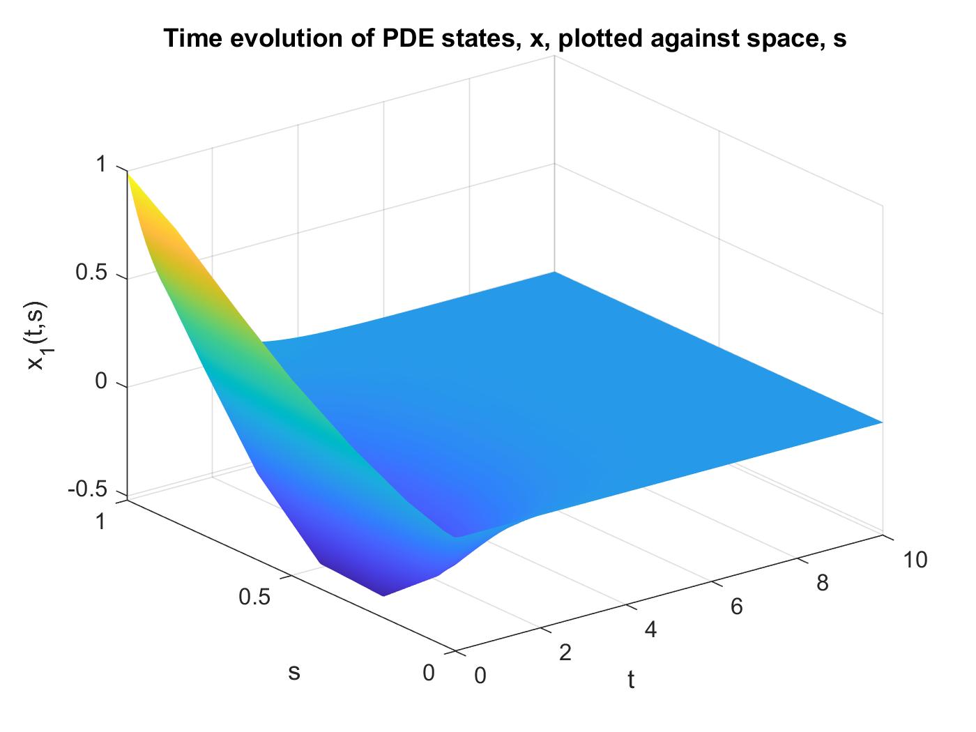
Figure 1: Ex. 26: Surface plot of closed loop response $\mathbf{x}(t,s)$ against $t$ and $s$ under the disturbance $w(t)=\sin(10t)/(10t)$

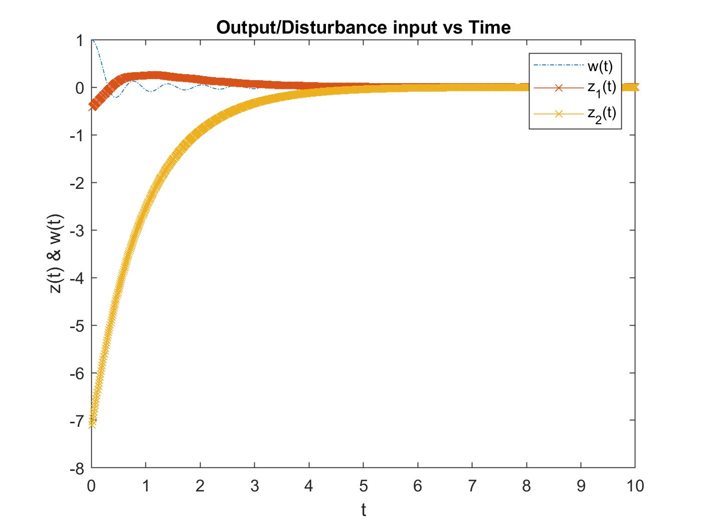
Figure 2: Ex. 26: Plot of output $z(t)=\int_{0}^{1}\mathbf{x}(t,s)ds$ against $t$ under the disturbance $w(t)=\sin(10t)/(10t)$

Example 27 (Wave equation).

Wave equation is a conservative system and stable. However, the states of the wave equation do not converge to zero with time, and hence, the wave PDE is not asymptotically stable. In this example, we use a dynamic controller to drive the states of the wave equation PDE via boundary inputs to zero. First, we perform a change of variable to cast the PDE in the standard form shown in Sec. III. Consider the wave equation with initial and boundary conditions specified below

$$\ddot{\eta}(t,s)=\partial_{s}^{2}\eta(t,s)+w(t),$$

$$\eta(0,s)=sin(\pi s),~{}~{}\dot{\eta}(0,s)=0,$$

$$\eta(t,0)=0,~{}~{}\partial_{s}\eta(t,1)=x(t),$$

$$\dot{x}(t)=-x(t)+u(t),$$

$$z(t)=\begin{bmatrix}\int_{0}^{1}\eta(t,s)ds\\ u(t)\end{bmatrix}$$ (48)

where $u$ is the input required to drive $w(t,\cdot)$ to zero through the coupling with the controller state $x(t)$, $z$ is the regulated output and $d$ is an $L_{2}$-bounded external disturbance. We use the change of variable $\mathbf{x}=col(\partial_{s}\eta,\dot{\eta})$ to obtain the following system in the standard form (as presented in Sec. III)

$$\begin{bmatrix}\dot{x}(t)\\ z(t)\end{bmatrix}=\begin{bmatrix}-1&0&1&0\\ \begin{bmatrix}0\\ 0\end{bmatrix}&\begin{bmatrix}0\\ 0\end{bmatrix}&\begin{bmatrix}0\\ 1\end{bmatrix}&\begin{bmatrix}1\\ 0\end{bmatrix}\end{bmatrix}\begin{bmatrix}x(t)\\ w(t)\\ u(t)\\ r(t)\end{bmatrix},$$

$$\dot{\mathbf{x}}(t,s)=\begin{bmatrix}0&1\\ 1&0\end{bmatrix}\partial_{s}\mathbf{x}(t,s)+\begin{bmatrix}0\\ 1\end{bmatrix}w(t),$$

$$r(t)=\int_{0}^{1}\begin{bmatrix}(1-s)&0\end{bmatrix}\mathbf{x}(t,s)ds,$$

$$\begin{bmatrix}0&1&0&0\\ 0&0&1&0\end{bmatrix}\begin{bmatrix}\mathbf{x}(t,0)\\ \mathbf{x}(t,1)\end{bmatrix}=\begin{bmatrix}0\\ 1\end{bmatrix}x(t).$$

Using PIETOOLS, we obtain a feedback law of the form $u(t)=\mathcal{K}\begin{bmatrix}x(t)\\ \mathbf{x}(t)\end{bmatrix}$ with an $H_{\infty}$-norm of $2.2\times 10^{4}$, where the $\mathcal{K}$ is a 4-PI operator as defined in Eq. (51). In Figures 3 and 4, we plot the response of the closed loop system for a disturbance input $w(t)=\sin(10t)/(10t)$ with initial conditions set to as $\sin(\pi s)$ for all PDE states and $0$ for ODE states.

$$\mathcal{K}=\mathcal{P}\left[\footnotesize\begin{array}[]{c|c}P&Q_{1}\\ \hline\cr 0&\{0\}\end{array}\right],\quad P=-0.17322,\quad Q_{1}(s)=10^{-3}\begin{bmatrix}Q_{11}(s)\\ Q_{12}(s)\end{bmatrix}$$ (51)

$$Q_{11}(s)=5s^{8}-20s^{7}+30s^{6}-20s^{5}-300s^{4}+600s^{3}$$

$$\qquad-700s^{2}+200s-8,$$

$$Q_{12}(s)=2s^{8}-7s^{7}+0.6s^{6}+6s^{5}-50s^{4}-200s^{3}$$

$$\qquad+800s^{2}-20s-400.$$

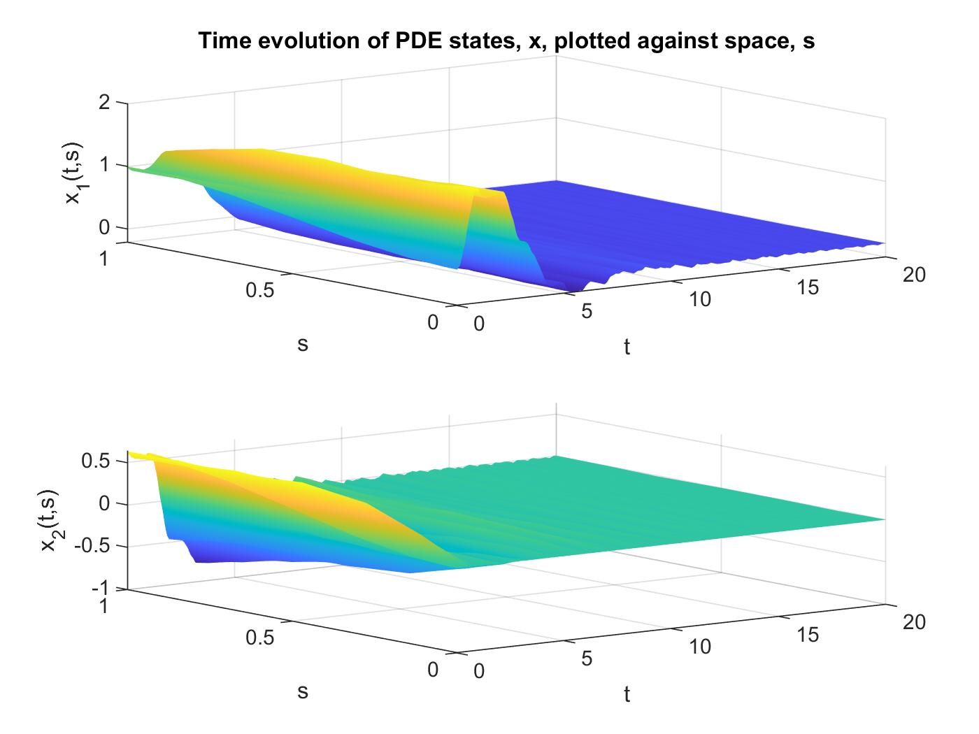
Figure 3: Ex. 27: Surface plot of closed loop response $\mathbf{x}(t,s)$ against $t$ and $s$ under the disturbance $w(t)=\sin(10t)/(10t)$

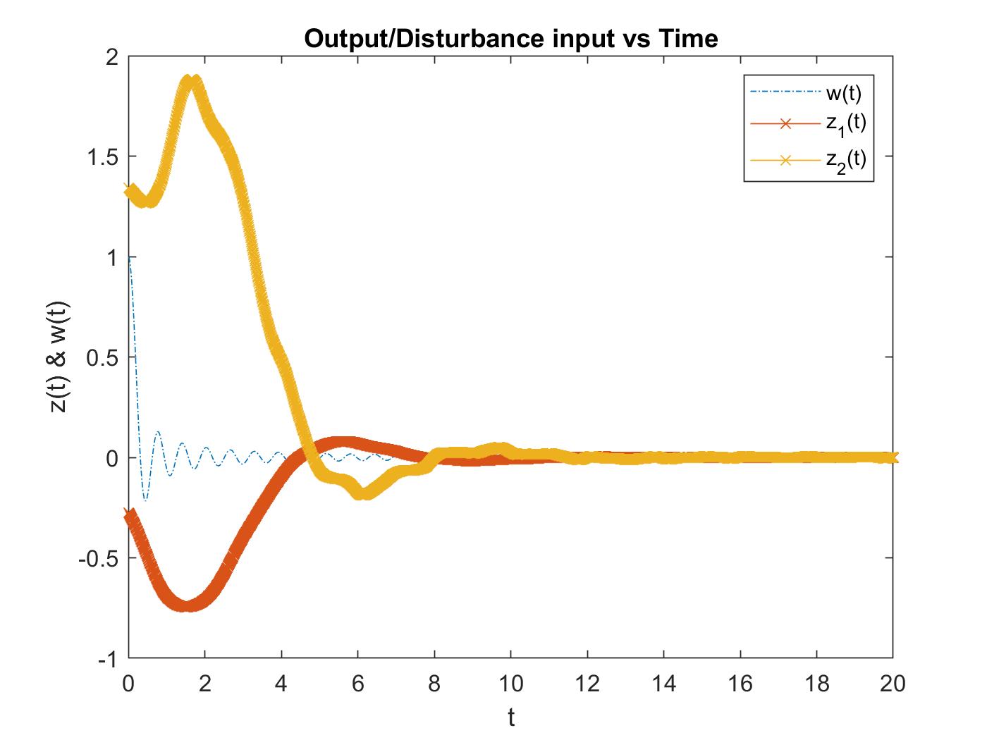
Figure 4: Ex. 27: Plot of output $z(t)=\int_{0}^{1}\eta(t,s)ds$ against $t$ under the disturbance $w(t)=\sin(10t)/(10t)$

XVII-C Stabilizing Boundary Controller

In this subsection, we present a numerical example where the LPI (32) was used to find a boundary control law using PIETOOLS. However, note that, due to the conservatism the optimization problem was solvable only when the stability parameter $\lambda$ of the reaction-diffusion PDE was close to stable values. For larger values of $\lambda$ the LPI was unable to find a feasible solution for low order polynomial parametrization of the decision variables $\mathcal{P}$ and $\mathcal{Z}$.

Example 28.

Consider the PDE in Example 24. Suppose $\lambda=10$. Then the system is unstable. This time, we use a static boundary input to stabilize the system as opposed to the dynamic boundary controller used in the previous examples. The goal of this exercise was to determine if the conservative LPI derived in Theorem 13 can perform better than the dynamic boundary controller approach. Given the PDE

$$\dot{\mathbf{x}}(t,s)=\lambda\mathbf{x}(t,s)+\partial_{s}^{2}\mathbf{x}(t,s)$$

$$\mathbf{x}(t,0)=0,~{}\mathbf{x}(t,1)=u(t),~{}\mathbf{x}(0,s)=sin(\pi s),$$

we try to find a control law $u(t)=\int_{a}^{b}K(s)\partial_{s}^{2}\mathbf{x}(t,s)ds$ by solving the LPI in Theorem 13. Preliminary tests indicate that conservatism of the Young’s inequality LPI is too high and a stabilizing static boundary controller could not be found for the PDE for large $\lambda$ as documented below.

$\lambda$	$\begin{matrix}\text{Dynamic}\\ \text{Boundary Control}\end{matrix}$	$\begin{matrix}\text{Static}\\ \text{Boundary control}\end{matrix}$
10	feasible	feasible
12	feasible	feasible
15	feasible	infeasible
30	feasible	infeasible

XVIII CONCLUSIONS

In this article, we solved the controller synthesis problem for a general class of linear ODE-PDEs by rewriting ODE-PDEs as PIEs and then using computational tools used in controller synthesis for PIEs. First, we presented a dual stability result for PIEs which allows us to formulate controller synthesis problem as convex optimization problems called as LPIs. The LPI result was then used to find stabilizing and $H_{\infty}$-optimal controllers for ODE-PDEs where the controllers act in the domain. Furthermore, we showed that the boundary control problem for ODE-PDEs lead to a PI inequality that is quadratic and provided a tightened PI inequality that can be written as an LPI. Finally, we use numerical examples to compare the conservatism of the method with other controller design techniques for ODE-PDEs.

Formulae to convert ODE-PDE to a PIE

$$n_{\mathbf{x}}=\sum_{i=0}^{N}n_{i},\quad n_{S_{i}}:=\sum_{j=i}^{N}n_{j}\quad n_{S}=\sum_{i=1}^{N}n_{S_{i}}\quad n_{i:j}:=\sum_{k=i}^{j}n_{k},$$

$$T_{i,j}(s)=\frac{s^{j-i}}{(j-i)!}\begin{bmatrix}0_{n_{Si}-n_{Sj}\times n_{Sj}}\\ I_{n_{Sj}}\end{bmatrix},\qquad T(s)=\begin{bmatrix}T_{1,1}(s)&T_{1,2}(s)&\cdots&T_{1,N}(s)\\ 0&T_{2,2}(s)&\cdots&T_{2,N}(s)\\ \vdots&\vdots&\ddots&\vdots\\ 0&0&\cdots&T_{N,N}(s)\end{bmatrix}\in\mathbb{R}^{n_{S}\times n_{S}},$$

$$U_{2i}=\begin{bmatrix}0_{n_{i}\times n_{i+1:N}}\\ I_{n_{i+1:N}}\end{bmatrix}\in\mathbb{R}^{n_{S_{i}}\times n_{S_{i+1}}},\qquad U_{2}=\begin{bmatrix}\text{diag}(U_{2,0},\cdots,U_{2,(N-1)})\\ 0_{n_{N}\times n_{S}}\end{bmatrix}\in\mathbb{R}^{\left(n_{\mathbf{x}}+n_{S}\right)\times n_{S}},$$

$$U_{1i}=\begin{bmatrix}I_{n_{i}}\\ 0_{n_{i+1:N}\times n_{i}}\end{bmatrix}\in\mathbb{R}^{n_{S_{i}}\times n_{i}},\qquad U_{1}=\begin{bmatrix}U_{10}&&\\ &\ddots&\\ &&U_{1N}\end{bmatrix}\in\mathbb{R}^{(n_{S}+n_{\mathbf{x}})\times n_{\mathbf{x}}},$$

$$Q_{i}(s)=\begin{bmatrix}0&\tau_{0}(s)I_{n_{i}}&&&\\ 0&&\tau_{1}(s)I_{n_{i+1}}&&\\ \vdots&&&\ddots&\\ 0&&&&\tau_{N-i}(s)I_{n_{N}}\end{bmatrix},\qquad Q(s)=\begin{bmatrix}Q_{1}(s)\\ \vdots\\ Q_{N}(s)\end{bmatrix}\in\mathbb{R}^{n_{S}\times n_{\mathbf{x}}},$$

$$B_{T}:=B\begin{bmatrix}T(0)\\ T(b-a)\end{bmatrix}\in\mathbb{R}^{n_{BC}\times n_{S}},\quad B_{Q}(s)=-B_{T}^{-1}B\begin{bmatrix}0\\ Q(b-s)\end{bmatrix},$$

$$G_{0}=\begin{bmatrix}I_{n_{0}}&\\ &0_{(n_{\mathbf{x}}-n_{0})}\end{bmatrix},\qquad G_{2}(s,\theta)=\begin{bmatrix}0\\ T_{1}(s-a)B_{Q}(\theta)\end{bmatrix},$$

$$G_{1}(s,\theta)=\begin{bmatrix}0\\ Q_{1}(s-\theta)\end{bmatrix}+G_{2}(s,\theta),\qquad G_{v}(s)=\begin{bmatrix}0\\ T_{1}(s-a)B_{T}^{-1}B_{v}\end{bmatrix},$$

$$R_{D,2}(s,\theta)=U_{2}T(s-a)B_{Q}(\theta)\qquad R_{D,1}(s,\theta)=R_{D,2}(s,\theta)+U_{2}Q(s-\theta)$$

$$\left[\begin{array}[]{c|c}D_{rv}&C_{rx}\\ \hline\cr B_{xv}&\{\hat{A}_{i}\}\end{array}\right]=\mathbf{P}_{c}^{4}\left(\left[\footnotesize\begin{array}[]{c|c}\begin{bmatrix}0&D_{rb}\end{bmatrix}&C_{r}\\ \hline\cr\begin{bmatrix}B_{xv}&B_{xb}\end{bmatrix}&\{A_{i}\}\end{array}\right],\left[\footnotesize\begin{array}[]{c|c}\begin{bmatrix}I_{n_{v}}\\ B_{T}^{-1}B_{v}\\ T(b-a)B_{T}^{-1}B_{v}\end{bmatrix}&\begin{bmatrix}0_{n_{r}\times n_{x}}\\ B_{Q}(s)\\ T(b-a)B_{Q}(s)+Q(b-s)\end{bmatrix}\\ \hline\cr U_{2}T(s-a)B_{T}^{-1}B_{v}&\{U_{1},R_{D,1},R_{D,2}\}\end{array}\right]\right)$$

$$\hat{\mathcal{T}}=\mathcal{P}\left[\footnotesize\begin{array}[]{c|c}\emptyset&\emptyset\\ \hline\cr\emptyset&\{G_{i}\}\end{array}\right],\qquad\mathcal{T}_{v}=\mathcal{P}\left[\footnotesize\begin{array}[]{c|c}\emptyset&\emptyset\\ \hline\cr G_{v}&\{\emptyset\}\end{array}\right],$$

$$\hat{\mathcal{A}}=\mathcal{P}\left[\footnotesize\begin{array}[]{c|c}\emptyset&\emptyset\\ \hline\cr\emptyset&\{\hat{A}_{i}\}\end{array}\right]\quad\mathcal{B}_{v}=\mathcal{P}\left[\footnotesize\begin{array}[]{c|c}\emptyset&\emptyset\\ \hline\cr B_{xv}&\{\emptyset\}\end{array}\right]\quad\mathcal{C}_{r}=\mathcal{P}\left[\footnotesize\begin{array}[]{c|c}\emptyset&C_{rx}\\ \hline\cr\emptyset&\{\emptyset\}\end{array}\right]\quad\mathcal{D}_{rv}=\mathcal{P}\left[\footnotesize\begin{array}[]{c|c}D_{rv}&\emptyset\\ \hline\cr\emptyset&\{\emptyset\}\end{array}\right]$$

$$\mathcal{T}=\begin{bmatrix}I_{n_{x}}&0\\ G_{v}C_{v}&\hat{\mathcal{T}}\end{bmatrix},\quad\mathcal{T}_{w}=\begin{bmatrix}0&0\\ G_{v}D_{vw}&0\end{bmatrix},\quad\mathcal{T}_{u}=\begin{bmatrix}0&0\\ G_{v}D_{vu}&0\end{bmatrix},$$

$$\mathcal{A}=\begin{bmatrix}A+B_{xr}\mathcal{D}_{rv}C_{v}&B_{xr}\mathcal{C}_{r}\\ \mathcal{B}_{v}C_{v}&\hat{\mathcal{A}}\end{bmatrix},\quad\mathcal{B}_{1}=\begin{bmatrix}B_{xw}+B_{xr}\mathcal{D}_{rv}D_{vw}\\ \mathcal{B}_{v}D_{vw}\end{bmatrix},\quad\mathcal{B}_{2}=\begin{bmatrix}B_{xu}+B_{xr}\mathcal{D}_{rv}D_{vu}\\ \mathcal{B}_{v}D_{vu}\end{bmatrix},$$

$$\mathcal{C}_{1}=\begin{bmatrix}C_{z}+D_{zr}\mathcal{D}_{rv}C_{v}&D_{zr}\mathcal{C}_{r}\end{bmatrix},\quad\mathcal{D}_{11}=D_{zw}+D_{zr}\mathcal{D}_{rv}D_{vw},\quad\mathcal{D}_{12}=D_{zu}+D_{zr}\mathcal{D}_{rv}D_{vu}.$$

Figure 5: Formulae based on parameters $\{n,\mathbf{G}_{\mathrm{b}},\mathbf{G}_{\mathrm{o}},\mathbf{G}_{\mathrm{p}}\}$.

XIX APPENDIX: Proof of Lemma 21

Lemma 29.

Suppose $P\in\mathbb{R}^{m\times m}$, $Q:[a,b]\to\mathbb{R}^{m\times n}$, $R_{0}:[a,b]\to\mathbb{R}^{n\times n}$ and $R_{1},R_{2}:[a,b]^{2}\to\mathbb{R}^{n\times n}$ are matrices and matrix-valued polynomials with $P$ and $\mathcal{P}_{\{H_{i}\}}$ invertible with the inverse being $\mathcal{P}_{\{L_{i}\}}$, where

$$H_{0}(s) =R_{0}(s),\quad H_{i}(s,\theta)=R_{i}(s,\theta)-Q(s)^{T}P^{-1}Q(\theta),$$

for $~{}i\in\{1,2\}$. Then, the inverse of $\mathcal{P}\left[\footnotesize\begin{array}[]{c|c}P&Q\\ \hline\cr Q^{T}&\{R_{0}\}\end{array}\right]$ is given by

$$\left(\mathcal{P}\left[\footnotesize\begin{array}[]{c|c}P&Q\\ \hline\cr Q^{T}&\{R_{i}\}\end{array}\right]\right)^{-1} =\mathcal{P}\left[\footnotesize\begin{array}[]{c|c}\hat{P}&\hat{Q}\\ \hline\cr\hat{Q}^{T}&\{\hat{R}_{i}\}\end{array}\right],$$

where $\hat{P},\hat{Q},\hat{R}_{i}$ are defined as

$$\hat{R}_{0}(s) =L_{0}(s),\quad\hat{R}_{i}(s,\theta)=L_{i}(s,\theta),\quad\text{for}~{}i\in\{1,2\},$$

$$\hat{P} =P^{-1}+P^{-1}\left(\int_{a}^{b}(Q(s)L_{0}(s)Q(s)^{T}+\int_{s}^{b}Q(\theta)L_{1}(\theta,s)Q(\theta)^{T}d\theta+\int_{a}^{s}Q(\theta)L_{2}(\theta,s)Q(\theta)^{T}d\theta\right)dsP^{-1}$$

$$\hat{Q}(s) =-P^{-1}\left(Q(s)L_{0}(s)+\int_{s}^{b}Q(\theta)L_{1}(\theta,s)d\theta+\int_{a}^{s}Q(\theta)L_{2}(\theta,s)d\theta\right).$$

Proof.

We prove this by verification of inverse. Let

$$\mathcal{P}\left[\footnotesize\begin{array}[]{c|c}A&B\\ \hline\cr B^{T}&\{C_{i}\}\end{array}\right]:=\mathcal{P}\left[\footnotesize\begin{array}[]{c|c}P&Q\\ \hline\cr Q^{T}&\{R_{i}\}\end{array}\right]\mathcal{P}\left[\footnotesize\begin{array}[]{c|c}\hat{P}&\hat{Q}\\ \hline\cr\hat{Q}^{T}&\{\hat{R}_{i}\}\end{array}\right].$$

Then, by the composition formulae for 4-PI operators, we have

$$A =P\hat{P}+\int_{a}^{b}Q(s)\hat{Q}^{T}(s)ds$$

$$=P\left(P^{-1}+P^{-1}\left(\int_{a}^{b}(Q(s)L_{0}(s)Q(s)^{T}+\int_{s}^{b}Q(\theta)L_{1}(\theta,s)Q(\theta)^{T}d\theta+\int_{a}^{s}Q(\theta)L_{2}(\theta,s)Q(\theta)^{T}d\theta\right)dsP^{-1}\right)$$

$$\quad-\int_{a}^{b}Q(s)\left(L_{0}(s)Q(s)^{T}+\int_{s}^{b}Q(\theta)L_{1}(\theta,s)Q(\theta)^{T}d\theta+\int_{a}^{s}Q(\theta)L_{2}(\theta,s)Q(\theta)^{T}d\theta\right)P^{-1}ds$$

$$=I.$$

Next, for $B$, we have the formula

$$B(s) =P\hat{Q}(s)+Q(s)\hat{R}_{0}(s)+\int_{s}^{b}Q(\theta)\hat{R}_{1}(\theta,s)\text{d}\theta+\int_{a}^{s}Q(\theta)\hat{R}_{2}(\theta,s)\text{d}\theta$$

$$P\hat{Q}(s)+Q(s)L_{0}(s)+\int_{s}^{b}Q(\theta)L_{1}(\theta,s)\text{d}\theta+\int_{a}^{s}Q(\theta)L_{2}(\theta,s)\text{d}\theta=0.$$

Lastly, for $C_{i}$, we have

$$C_{0}(s) =R_{0}(s)\hat{R}_{0}(s)=R_{0}(s)L_{0}(s)=R_{0}(s)H_{0}(s)^{-1}=R_{0}(s)R_{0}(s)^{-1}=I,$$

$$C_{1}(s,\theta) =Q(s)^{T}\hat{Q}(\theta)+R_{0}(s)\hat{R}_{1}(s,\theta)+R_{1}(s,\theta)\hat{R}_{0}(\theta)+\int_{a}^{\theta}R_{1}(s,\eta)\hat{R}_{2}(\eta,\theta)\text{d}\eta+\int_{\theta}^{s}R_{1}(s,\eta)\hat{R}_{1}(\eta,\theta)\text{d}\eta$$

$$\qquad+\int_{s}^{b}R_{2}(s,\eta)\hat{R}_{1}(\eta,\theta)\text{d}\eta$$

$$=-Q(s)^{T}P^{-1}Q(\theta)L_{0}(\theta)-Q(s)^{T}P^{-1}\left(\int_{\theta}^{b}Q(s)L_{1}(s,\theta)ds+\int_{a}^{\theta}Q(s)L_{2}(s,\theta)ds\right)$$

$$\qquad+R_{0}(s)L_{1}(s,\theta)+R_{1}(s,\theta)L_{0}(\theta)+\int_{a}^{\theta}R_{1}(s,\eta)L_{2}(\eta,\theta)\text{d}\eta+\int_{\theta}^{s}R_{1}(s,\eta)L_{1}(\eta,\theta)\text{d}\eta$$

$$\qquad+\int_{s}^{b}R_{2}(s,\eta)L_{1}(\eta,\theta)\text{d}\eta=0.$$

Then, clearly, $\mathcal{P}\left[\footnotesize\begin{array}[]{c|c}P&Q\\ \hline\cr Q^{T}&\{R_{i}\}\end{array}\right]\mathcal{P}\left[\footnotesize\begin{array}[]{c|c}\hat{P}&\hat{Q}\\ \hline\cr\hat{Q}^{T}&\{\hat{R}_{i}\}\end{array}\right]=I_{L_{2}}.$ Likewise, we can show that $\mathcal{P}\left[\footnotesize\begin{array}[]{c|c}\hat{P}&\hat{Q}\\ \hline\cr\hat{Q}^{T}&\{\hat{R}_{i}\}\end{array}\right]\mathcal{P}\left[\footnotesize\begin{array}[]{c|c}P&Q\\ \hline\cr Q^{T}&\{R_{i}\}\end{array}\right]=I_{L_{2}}$. ∎

XX APPENDIX: Proof of Theorem 18

Theorem 30.

Suppose there exist $\epsilon>0,\gamma>0$, bounded linear operators $\mathcal{P}:\mathbb{R}L_{2}^{m,n}[a,b]\to\mathbb{R}L_{2}^{m,n}[a,b]$ and $\mathcal{Z}:\mathbb{R}L_{2}^{m,n}[a,b]\to\mathbb{R}^{p}$, such that $\mathcal{P}$ is self-adjoint, coercive and $\mathcal{P}^{D}\preccurlyeq 0$ Then, for any $w\in L_{2}$, for $u(t)=\mathcal{K}\mathbf{x}(t)$ where $\mathcal{K}=\mathcal{ZP}^{-1}$, any $\mathbf{v}$ and $z$ that satisfy the PIE (XV) also satisfy $\left\|z\right\|_{L_{2}}\leq\gamma\left\|w\right\|_{L_{2}}$.

Proof.

Let $V(t)=\left\langle{\left(\mathcal{T}+\mathcal{T}_{u}\mathcal{K}\right)^{*}x(t)},{\mathcal{P}\left(\mathcal{T}+\mathcal{T}_{u}\mathcal{K}\right)^{*}x(t)}\right\rangle_{H}$ be a candidate for Lyapunov function where $x\in\mathbb{R}L_{2}^{m,n}$ and $z\in R^{l}$ satisfy the dual PIE (XV). Since $\mathcal{P}$ is coercive and bounded, there exists $\alpha>0$ and $\beta>0$ such that

$$\alpha\left\|\left(\mathcal{T}+\mathcal{T}_{u}\mathcal{K}\right)^{*}x\right\|_{H}\leq V(x)\leq\beta\left\|\left(\mathcal{T}+\mathcal{T}_{u}\mathcal{K}\right)^{*}x\right\|_{H}\quad\forall x\in Z.$$

The time derivative of $V(t)$ along the solutions of Eq. (XV) is given by

$$\dot{V}(t) =\left\langle{\left(\mathcal{T}+\mathcal{T}_{u}\mathcal{K}\right)^{*}x(t)},{\mathcal{P}(\mathcal{A}+\mathcal{B}_{2}\mathcal{K})^{*}x(t)}\right\rangle_{H}+\left\langle{(\mathcal{A}+\mathcal{B}_{2}\mathcal{K})^{*}x(t)},{\mathcal{P}\left(\mathcal{T}+\mathcal{T}_{u}\mathcal{K}\right)^{*}x(t)}\right\rangle_{H}$$

$$~{}~{}\quad+\left\langle{\left(\mathcal{T}+\mathcal{T}_{u}\mathcal{K}\right)^{*}x(t)},{\mathcal{P}(\mathcal{C}+\mathcal{D}_{12}\mathcal{K})^{*}w(t)}\right\rangle_{H}+\left\langle{(\mathcal{C}+\mathcal{D}_{12}\mathcal{K})^{*}w(t)},{\mathcal{P}\left(\mathcal{T}+\mathcal{T}_{u}\mathcal{K}\right)^{*}x(t)}\right\rangle_{H}$$

$$=\left\langle{x(t)},{\left(\mathcal{T}\mathcal{P}\mathcal{A}^{*}+\mathcal{A}\mathcal{P}\mathcal{T}^{*}+\mathcal{A}\mathcal{Z}^{*}\mathcal{T}_{u}^{*}+\mathcal{T}_{u}\mathcal{Z}\mathcal{A}^{*}+\mathcal{T}\mathcal{Z}^{*}\mathcal{B}_{2}^{*}+\mathcal{B}_{2}\mathcal{Z}\mathcal{T}^{*}\right)x(t)}\right\rangle_{H}$$

$$\quad+\left\langle{x(t)},{\left(\mathcal{T}_{u}\mathcal{Z}\mathcal{P}^{-1}\mathcal{Z}^{*}\mathcal{B}_{2}^{*}+\mathcal{B}_{2}\mathcal{Z}\mathcal{P}^{-1}\mathcal{Z}^{*}\mathcal{T}_{u}^{*}\right)x(t)}\right\rangle_{H}$$

$$~{}~{}\quad+\left\langle{x(t)},{\left(\mathcal{T}\mathcal{P}\mathcal{C}_{1}^{*}+\mathcal{T}_{u}\mathcal{Z}\mathcal{C}_{1}^{*}+\mathcal{T}\mathcal{Z}^{*}\mathcal{D}_{12}^{*}\right)w(t)}\right\rangle_{H}+\left\langle{w(t)},{\left(\mathcal{C}_{1}\mathcal{P}\mathcal{T}^{*}+\mathcal{C}_{1}\mathcal{Z}^{*}\mathcal{T}_{u}^{*}+\mathcal{D}_{12}\mathcal{Z}\mathcal{T}^{*}\right)x(t)}\right\rangle_{H}$$

$$\qquad+\left\langle{x(t)},{\mathcal{T}_{u}\mathcal{Z}\mathcal{P}^{-1}\mathcal{Z}^{*}\mathcal{D}_{12}^{*}w(t)}\right\rangle_{H}+\left\langle{w(t)},{\mathcal{D}_{12}\mathcal{Z}\mathcal{P}^{-1}\mathcal{Z}^{*}\mathcal{T}_{u}^{*}x(t)}\right\rangle_{H}$$

where we have used a change of variable $\mathcal{KP}=\mathcal{Z}$. Furthermore, using Lemma 14, we have

$$\dot{V}(t) \leq\left\langle{x(t)},{\left(\mathcal{T}\mathcal{P}\mathcal{A}^{*}+\mathcal{A}\mathcal{P}\mathcal{T}^{*}+\mathcal{A}\mathcal{Z}^{*}\mathcal{T}_{u}^{*}+\mathcal{T}_{u}\mathcal{Z}\mathcal{A}^{*}+\mathcal{T}\mathcal{Z}^{*}\mathcal{B}_{2}^{*}+\mathcal{B}_{2}\mathcal{Z}\mathcal{T}^{*}\right)x(t)}\right\rangle$$

$$\quad+\left\langle{x(t)},{\left(\mathcal{T}_{u}\mathcal{Z}\mathcal{P}^{-1}\mathcal{Z}^{*}\mathcal{T}_{u}^{*}+\mathcal{B}_{2}\mathcal{Z}\mathcal{P}^{-1}\mathcal{Z}^{*}\mathcal{B}_{2}^{*}\right)x(t)}\right\rangle$$

$$~{}~{}\quad+\left\langle{x(t)},{\left(\mathcal{T}\mathcal{P}\mathcal{C}_{1}^{*}+\mathcal{T}_{u}\mathcal{Z}\mathcal{C}_{1}^{*}+\mathcal{T}\mathcal{Z}^{*}\mathcal{D}_{12}^{*}\right)w(t)}\right\rangle+\left\langle{w(t)},{\left(\mathcal{C}_{1}\mathcal{P}\mathcal{T}^{*}+\mathcal{C}_{1}\mathcal{Z}^{*}\mathcal{T}_{u}^{*}+\mathcal{D}_{12}\mathcal{Z}\mathcal{T}^{*}\right)x(t)}\right\rangle$$

$$\qquad+\left\langle{x(t)},{\mathcal{T}_{u}\mathcal{Z}\mathcal{P}^{-1}\mathcal{Z}^{*}\mathcal{T}_{u}^{*}x(t)}\right\rangle+\left\langle{w(t)},{\mathcal{D}_{12}\mathcal{Z}\mathcal{P}^{-1}\mathcal{Z}^{*}\mathcal{D}_{12}^{*}w(t)}\right\rangle$$

Suppose, $\mathcal{P}$ and $\mathcal{Z}$ satisfy the LPI (44). Then, by taking Schur’s complement, the following inequality is equivalent to LPI (44).

$$\begin{bmatrix}-\gamma&\left(\mathcal{C}_{1}\mathcal{P}\mathcal{T}^{*}+\mathcal{C}_{1}\mathcal{Z}^{*}\mathcal{T}_{u}^{*}+\mathcal{D}_{12}\mathcal{Z}\mathcal{T}^{*}\right)\\ (\cdot)^{*}&(\cdot)^{*}+\left(\mathcal{TPA}^{*}++\mathcal{T}_{u}\mathcal{Z}\mathcal{A}^{*}+\mathcal{T}\mathcal{Z}^{*}\mathcal{B}_{2}^{*}\right)\end{bmatrix}+\begin{bmatrix}\mathcal{D}_{11}^{*}&\mathcal{B}_{1}^{*}\\ \mathcal{Z}^{*}\mathcal{D}_{12}^{*}&0\\ 0&\sqrt{2}\mathcal{Z}^{*}\mathcal{T}_{u}^{*}\\ 0&\mathcal{Z}^{*}\mathcal{B}_{2}^{*}\end{bmatrix}^{*}\begin{bmatrix}-\gamma&0&0&0\\ 0&-\mathcal{P}&0&0\\ 0&0&-\mathcal{P}&0\\ 0&0&0&-\mathcal{P}\end{bmatrix}^{-1}\begin{bmatrix}\mathcal{D}_{11}^{*}&\mathcal{B}_{1}^{*}\\ \mathcal{Z}^{*}\mathcal{D}_{12}^{*}&0\\ 0&\sqrt{2}\mathcal{Z}^{*}\mathcal{T}_{u}^{*}\\ 0&\mathcal{Z}^{*}\mathcal{B}_{2}^{*}\end{bmatrix}\prec 0$$

For any given $w(t)\in\mathbb{R}^{p}$, let $z(t)$ and $\mathbf{x}(t)\in Z$ satisfy Eq. (XV). Then,

$$0>\left\langle{\begin{bmatrix}w(t)\\ \mathbf{x}(t)\end{bmatrix}},{\begin{bmatrix}-\gamma&\left(\mathcal{C}_{1}\mathcal{P}\mathcal{T}^{*}+\mathcal{C}_{1}\mathcal{Z}^{*}\mathcal{T}_{u}^{*}+\mathcal{D}_{12}\mathcal{Z}\mathcal{T}^{*}\right)\\ (\cdot)^{*}&(\cdot)^{*}+\left(\mathcal{TPA}^{*}++\mathcal{T}_{u}\mathcal{Z}\mathcal{A}^{*}+\mathcal{T}\mathcal{Z}^{*}\mathcal{B}_{2}^{*}\right)\end{bmatrix}\begin{bmatrix}w(t)\\ \mathbf{x}(t)\end{bmatrix}}\right\rangle$$

$$\quad+\left\langle{\begin{bmatrix}w(t)\\ \mathbf{x}(t)\end{bmatrix}},{\begin{bmatrix}\mathcal{D}_{11}^{*}&\mathcal{B}_{1}^{*}\\ \mathcal{Z}^{*}\mathcal{D}_{12}^{*}&0\\ 0&\sqrt{2}\mathcal{Z}^{*}\mathcal{T}_{u}^{*}\\ 0&\mathcal{Z}^{*}\mathcal{B}_{2}^{*}\end{bmatrix}^{*}\begin{bmatrix}-\gamma&0&0&0\\ 0&-\mathcal{P}&0&0\\ 0&0&-\mathcal{P}&0\\ 0&0&0&-\mathcal{P}\end{bmatrix}^{-1}\begin{bmatrix}\mathcal{D}_{11}^{*}&\mathcal{B}_{1}^{*}\\ \mathcal{Z}^{*}\mathcal{D}_{12}^{*}&0\\ 0&\sqrt{2}\mathcal{Z}^{*}\mathcal{T}_{u}^{*}\\ 0&\mathcal{Z}^{*}\mathcal{B}_{2}^{*}\end{bmatrix}\begin{bmatrix}w(t)\\ \mathbf{x}(t)\end{bmatrix}}\right\rangle$$

$$=\left\langle{\mathbf{x}(t)},{\left(\mathcal{T}\mathcal{P}\mathcal{A}^{*}+\mathcal{A}\mathcal{P}\mathcal{T}^{*}+\mathcal{A}\mathcal{Z}^{*}\mathcal{T}_{u}^{*}+\mathcal{T}_{u}\mathcal{Z}\mathcal{A}^{*}+\mathcal{T}\mathcal{Z}^{*}\mathcal{B}_{2}^{*}+\mathcal{B}_{2}\mathcal{Z}\mathcal{T}^{*}\right)\mathbf{x}(t)}\right\rangle$$

$$\quad+\left\langle{\mathbf{x}(t)},{\left(\mathcal{T}\mathcal{P}\mathcal{C}_{1}^{*}+\mathcal{T}_{u}\mathcal{Z}\mathcal{C}_{1}^{*}+\mathcal{T}\mathcal{Z}^{*}\mathcal{D}_{12}^{*}\right)w(t)}\right\rangle+\left\langle{w(t)},{\left(\mathcal{C}_{1}\mathcal{P}\mathcal{T}^{*}+\mathcal{C}_{1}\mathcal{Z}^{*}\mathcal{T}_{u}^{*}+\mathcal{D}_{12}\mathcal{Z}\mathcal{T}^{*}\right)\mathbf{x}(t)}\right\rangle-\gamma\left\|w(t)\right\|^{2}$$

$$~{}~{}\quad+\frac{1}{\gamma}\left\|z(t)\right\|^{2}+\left\langle{\mathbf{x}(t)},{\left(\mathcal{T}_{u}\mathcal{Z}\mathcal{P}^{-1}\mathcal{Z}^{*}\mathcal{T}_{u}^{*}+\mathcal{B}_{2}\mathcal{Z}\mathcal{P}^{-1}\mathcal{Z}^{*}\mathcal{B}_{2}^{*}\right)\mathbf{x}(t)}\right\rangle$$

$$\qquad+\left\langle{\mathbf{x}(t)},{\mathcal{T}_{u}\mathcal{Z}\mathcal{P}^{-1}\mathcal{Z}^{*}\mathcal{T}_{u}^{*}\mathbf{x}(t)}\right\rangle+\left\langle{w(t)},{\mathcal{D}_{12}\mathcal{Z}\mathcal{P}^{-1}\mathcal{Z}^{*}\mathcal{D}_{12}^{*}w(t)}\right\rangle\geq\dot{V}(t)-\gamma\left\|w(t)\right\|^{2}+\frac{1}{\gamma}\left\|z(t)\right\|^{2}$$

Then, for any $t>0$,

$$\dot{V}(t)-\gamma\left\|w(t)\right\|^{2}+\frac{1}{\gamma}\left\|z(t)\right\|^{2}<0.$$

Integrating forward in time with the initial condition $\mathbf{x}(0)=0$, we obtain

$$V(T)+\frac{1}{\gamma}\int_{0}^{T}\left\|z(t)\right\|^{2}dt\leq\gamma\int_{0}^{T}\left\|w(t)\right\|^{2}dt$$

which can be further simplified by using the fact $V(t)>0$ for any $t$, resulting in the constraint

$$\frac{1}{\gamma}\int_{0}^{T}\left\|z(t)\right\|^{2}dt\leq\gamma\int_{0}^{T}\left\|w(t)\right\|^{2}dt.$$

Then, by taking the limit $t\to\infty$, we get $\left\|z\right\|_{L_{2}}^{2}\leq\gamma^{2}\left\|w\right\|_{L_{2}}^{2}$. Using Theorem 7, the dual PIE of Eq. (XV) has the same bound on $L_{2}$-gain from input to output. In other words, for $w\in L_{2}$, any $\mathbf{x}$ and $z$ that satisfy equations Eq. (XV) with $u=\mathcal{K}\mathbf{x}$ and $\mathcal{K}=\mathcal{Z}\mathcal{P}^{-1}$, also satisfy the constraint $\left\|z\right\|_{L_{2}}\leq\gamma\left\|w\right\|_{L_{2}}$. ∎

XXI APPENDIX: Proof of Theorem 23

thm Given an coupled ODE-PDE defined by the parameters $\{n,\mathbf{G}_{\mathrm{b}},\mathbf{G}_{\mathrm{o}},\mathbf{G}_{\mathrm{p}}\}$, suppose there exist $\gamma>0$, bounded linear operators $\mathcal{P}:\mathbb{R}L_{2}^{m,n}[a,b]\to\mathbb{R}L_{2}^{m,n}[a,b]$ and $\mathcal{Z}:\mathbb{R}L_{2}^{m,n}[a,b]\to\mathbb{R}^{p}$, such that $\mathcal{P}$ is self-adjoint, coercive and

$$\begin{bmatrix}-\gamma I&\mathcal{D}_{11}&(\mathcal{C}_{1}\mathcal{P}+\mathcal{D}_{12}\mathcal{Z})\mathcal{T}^{*}\\ (\cdot)^{*}&-\gamma I&\mathcal{B}_{1}^{*}\\ (\cdot)^{*}&(\cdot)^{*}&(\cdot)^{*}+\mathcal{T}(\mathcal{A}\mathcal{P}+\mathcal{B}_{2}\mathcal{Z})^{*}\end{bmatrix}\preccurlyeq 0$$ (52)

where $\mathcal{T},\mathcal{A},\mathcal{B}_{1},\mathcal{B}_{2},\mathcal{C}_{1},\mathcal{D}_{11},\mathcal{D}_{12}$ are as defined in Eq. Block 5. Then, for any $w\in L_{2}$, for

$$u(t)=K_{0}x(t)+\int_{a}^{b}K_{1}(s)(\mathcal{D}^{f}\mathbf{x})(t,s)ds$$

any $\{x,\mathbf{x},z,y\}$ that satisfy the ODE-PDE (III) also satisfy $\left\|z\right\|_{L_{2}}\leq\gamma\left\|w\right\|_{L_{2}}$ with zero initial conditions where $K_{0}$ and $K_{1}$ are as defined in Corollary 22 and $\mathcal{D}^{f}\mathbf{x}=\text{col}(\mathbf{x}_{0},\partial_{s}\mathbf{x}_{1},\cdots,\partial_{s}^{N}\mathbf{x}_{N})$. thm

Proof.

Let $\gamma>0$, $\mathcal{P}:\mathbb{R}L_{2}^{m,n}[a,b]\to\mathbb{R}L_{2}^{m,n}[a,b]$ and $\mathcal{Z}:\mathbb{R}L_{2}^{m,n}[a,b]\to\mathbb{R}^{p}$ be such that $\mathcal{P}$ is self-adjoint, coercive and

$$\begin{bmatrix}-\gamma I&\mathcal{D}_{11}&(\mathcal{C}_{1}\mathcal{P}+\mathcal{D}_{12}\mathcal{Z})\mathcal{T}^{*}\\ (\cdot)^{*}&-\gamma I&\mathcal{B}_{1}^{*}\\ (\cdot)^{*}&(\cdot)^{*}&(\cdot)^{*}+\mathcal{T}(\mathcal{A}\mathcal{P}+\mathcal{B}_{2}\mathcal{Z})^{*}\end{bmatrix}\preccurlyeq 0$$ (53)

where $\mathcal{T},\mathcal{A},\mathcal{B}_{1},\mathcal{B}_{2},\mathcal{C}_{1},\mathcal{D}_{11},\mathcal{D}_{12}$ are as defined in Eq. Block 5 for given parameters $\{n,\mathbf{G}_{\mathrm{b}},\mathbf{G}_{\mathrm{o}},\mathbf{G}_{\mathrm{p}}\}$.

Then from Theorem 17, any $\mathbf{x}_{f}$ and $z$ that satisfy the PIE (IV) for any $w\in L_{2}$, for $u(t)=\mathcal{ZP}^{-1}\mathbf{x}_{f}(t)$ also satisfy $\left\|z\right\|_{L_{2}}\leq\gamma\left\|w\right\|_{L_{2}}$. From Corollary 6.1 of [17], $\text{col}(x,\mathbf{x}):=\mathcal{T}\mathbf{x}_{f}$ and $z$ satisfy the ODE-PDE defined by $\{n,\mathbf{G}_{\mathrm{b}},\mathbf{G}_{\mathrm{o}},\mathbf{G}_{\mathrm{p}}\}$ for zero initial conditions and inputs $w$ and

$$u(t)=\mathcal{ZP}^{-1}\mathbf{x}_{f}(t)=\mathcal{ZP}^{-1}\begin{bmatrix}x(t)\\ \mathcal{D}^{f}\mathbf{x}(t)\end{bmatrix}=K_{0}x(t)+\int_{a}^{b}K_{1}(s)(\mathcal{D}^{f}\mathbf{x})(t,s)ds$$

while also satisfying $\left\|z\right\|_{L_{2}}\leq\gamma\left\|w\right\|_{L_{2}}$. ∎

References

• [1] P. Apkarian and D. Noll. Boundary control of partial differential equations using frequency domain optimization techniques. Systems & Control Letters, 135:104577, 2020.
• [2] S. Boyd, L. El Ghaoui, E. Feron, and V. Balakrishnan. Linear matrix inequalities in system and control theory, volume 15. SIAM, 1994.
• [3] S. S. Collis and M. Heinkenschloss. Analysis of the streamline upwind/Petrov-Galerkin method applied to the solution of optimal control problems. CAAM TR02-01, 108, 2002.
• [4] R. F. Curtain and H. J. Zwart. An Introduction to Infinite-dimensional Linear Systems Theory. Springer-Verlag New York, 1995.
• [5] A. Das, S. Shivakumar, S. Weiland, and M. Peet. ${H}_{\infty}$ optimal estimation for linear coupled PDE systems. In Proceedings of the IEEE Conference on Decision and Control, 2019.
• [6] I. M. Gelf́and and G. E. Shilov. Generalized functions. AMS Chelsea Publishing, 3, 1976.
• [7] I. Gohberg, S. Goldberg, and M. A. Kaashoek. Classes of linear operators Vol. I, volume 63. Birkhäuser, 2013.
• [8] K. Ito and S. Ravindran. Optimal control of thermally convected fluid flows. SIAM Journal on Scientific Computing, 19(6):1847–1869, 1998.
• [9] K. Ito and S. Ravindran. A reduced basis method for control problems governed by PDEs. In Control and estimation of distributed parameter systems, pages 153–168. Springer, 1998.
• [10] I. Karafyllis and M. Krstic. Input-to-state stability for PDEs. Springer, 2019.
• [11] M. Krstic and A. Smyshlyaev. Boundary control of PDEs: A course on backstepping designs, volume 16. SIAM, 2008.
• [12] K. Lenz, H. Ozbay, A. Tannenbaum, J. Turi, and B. Morton. Robust control design for a flexible beam using a distributed-parameter ${H}_{\infty}$-method. In Proceedings of the IEEE Conference on Decision and Control, pages 2673–2678, 1989.
• [13] M. Peet. A dual to Lyapunov’s second method for linear systems with multiple delays and implementation using SOS. IEEE Transactions on Automatic Control, 64(3):944 – 959, 2019.
• [14] M. Peet. A convex solution of the ${H}_{\infty}$-optimal controller synthesis problem for multidelay systems. SIAM Journal on Control and Optimization, 58(3):1547–1578, 2020.
• [15] M. Peet. A partial integral equation (PIE) representation of coupled linear PDEs and scalable stability analysis using LMIs. Automatica, 125:109473, 2021.
• [16] S. Shivakumar, A. Das, S. Weiland, and M. Peet. Duality and ${H}_{\infty}$-optimal control of coupled ODE-PDE systems. pages 5689–5696, 2020.
• [17] S. Shivakumar, A. Das, S. Weiland, and M. Peet. Extension of the partial integral equation representation to GPDE input-output systems. arXiv preprint arXiv:2205.03735, 2022.
• [18] S. Shivakumar, D. Jagt, and M. Peet. PIETOOLS. https://github.com/CyberneticSCL/PIETOOLS, 2019.
• [19] S. Shivakumar and M. Peet. Computing input-ouput properties of coupled linear PDE systems. In American Control Conference, pages 606–613. IEEE, 2019.
• [20] O. Toker and H. Ozbay. ${H}_{\infty}$-optimal and suboptimal controllers for infinite dimensional SISO plants. IEEE Transactions on Automatic Control, 40(4):751–755, 1995.
• [21] A. Zemouche, R. Rajamani, B. Boulkroune, H. Rafaralahy, and M. Zasadzinski. ${H}_{\infty}$ circle criterion observer design for lipschitz nonlinear systems with enhanced LMI conditions. In American Control Conference, pages 131–136. IEEE, 2016.