The Ghost of Performance Reproducibility Past

Abstract

The importance of ensemble computing is well established. However, executing ensembles at scale introduces interesting performance fluctuations that have not been well investigated. In this paper, we trace our experience uncovering performance fluctuations of ensemble applications (primarily constituting a workflow of GROMACS tasks), and unsuccessful attempts, so far, at trying to discern the underlying cause(s) of performance fluctuations. Is the failure to discern the causative or contributing factors a failure of capability? Or imagination? Do the fluctuations have their genesis in some inscrutable aspect of the system or software? Does it warrant a fundamental reassessment and rethinking of how we assume and conceptualize performance reproducibility? Answers to these questions are not straightforward, nor are they immediate or obvious. We conclude with a discussion about the performance of ensemble applications and ruminate over the implications for how we define and measure application performance.

I Introduction

Scientific high-performance computing (HPC) has focused on a workload’s functionality, scale, and performance with a single large task. However, the end of Dennard scaling, coupled with the realities of post-Moore parallelism, places increasingly severe limitations on the ability of a single monolithic task to achieve significant performance gains on large-scale parallel machines. In response to these challenges, scientific workflows have emerged as an important way of developing scientific applications on HPC platforms [1]. The coupling of AI to traditional HPC simulations is further increasing the performance and the sophistication of scientific workflow applications [2, 3].

Ensemble computing represents a particular case of workflows in which multiple copies of the same application are executed concurrently but independently. Ensemble-based applications have been used to generate improved scientific insight in multiple domains [4, 3, 5]. Today, ensemble-based applications executing on HPC platforms orchestrate 100s to 1000s of, individual tasks. Typically, each task is a scientific simulation implemented as a parallel MPI program spanning one or more distributed computing nodes. Further, the tasks can be heterogeneous regarding the application they represent and the computing resources to which they are mapped. Applications on the horizon [6] will require the concurrent execution of $10^{6}-10^{8}$ MPI tasks, the implications of which are many-fold and profound [7]

This work investigates the issue of the performance of an ensemble of tasks. In particular, it explores variability in the performance (as measured by the time-to-execution) of a set of otherwise identical tasks executed concurrently. Contrary to expectation, individual tasks did not have identical times-to-execution. The variability in runtime is seemingly independent of the specific executable and time-invariant (viz., state-of-the HPC machine). This paper builds upon and extends the result earlier identified  [8, 9]. Whether the execution time of otherwise identical tasks is indeed scale and time invariant, and independent of the specific task remain open questions.

To address these open questions, we investigate the performance of an ensemble of tasks, and measure the performance of an individual task taken from a set of otherwise identical tasks. We also evaluate the performance of the same set of tasks (workload) run at different instances of time. Lastly, we investigate the performance variability as a function of the workload size (i.e., the number of tasks).

The key contributions of this experience paper are: 1. Demonstrating and investigating performance variability of individual tasks that are part of a set of concurrently executing tasks; 2. Characterizing spatio-temporal aspects of the performance variability; 3. Design of experiments to investigate and narrow the possible causes of performance variability; 4. Postulating possible causes of performance variability and challenges in establishing performance reproducibility; and 5. Synthesizing the insight gained towards a nuanced yet generalized perspective of performance and performance reproducibility.

II Characterizing Performance Variation in GROMACS Ensembles

Homogeneous ensemble execution typically consists of simultaneously executing copies of the same program (ensemble task) on different input decks, representing for example, different initial conditions or input execution parameters. When input decks are different, individual ensemble tasks may execute different code paths leading to some natural variation in the individual task runtime. However, when the ensemble tasks execute identical input decks on identical resource allocations, any variation in task performance must result from system (exogenous) factors. Examples of these system factors known to cause application performance variation include processor variability [10], inter-job network interference [11], and operating system (OS) noise [12].

Experiments in Section II assumes that all tasks in the workload exactly concurrently fit in the allocated node resources. In such a scenario, makespan or the total execution time of the workload is affected by the task runtime variation arising from system (exogenous) factors. Two questions arise in this scenario: Q-1 What is the range of the execution times of individual ensemble tasks? Equally, how much do system factors affect the individual task runtime? Q-2 What is the range of the makespan itself? Equally, how much do system factors cause the makespan to vary across identical ensemble workload executions?

Even if the makespan itself does not vary significantly across ensemble workload executions, a large range of task runtimes within an ensemble workload execution can waste computing resources, because the workload does not complete until the last task has finished executing. Characterizing the degree to which system factors affect individual task performance and the makespan can help the understanding of these system (exogenous) factors (OS noise, inter-job interference, processor variability) and how they affect particular applications. This study presents our observations on executing GROMACS ensemble workloads on the Theta cluster at the Argonne Leadership Computing Facility. GROMACS was chosen partly because it is frequently executed as a part of ensemble workflows and partly because of our familiarity with it. In particular, we pay special attention to the methodology employed to: (1) characterize the performance variation observed from executing large-scale GROMACS ensembles, and (2) systematically narrow down the list of the potential system (exogenous) factors responsible for the behavior.

II-A The Observation That We Seek to Characterize

Figure 1 captures the behavior we seek to characterize and investigate. A total of 2,500 GROMACS ensemble tasks belonging to ensemble workloads spread across 10, 256-node batch jobs. Each of these GROMACS tasks employs 64 MPI ranks and executes 100,000 simulation timesteps with OpenMP support turned off. By default, checkpointing is enabled once every minute of wallclock execution time. Further, these tasks operate on identical input decks and execute on identical resource allocations (single, 64-core Theta KNL node). The task time-to-execution displays 16% of a difference between the runtimes for the fastest and the slowest tasks. The experimental setup would imply that the system (exogenous) factors are solely responsible for causing the variation in task performance, requiring further investigation and root cause analysis.

The observations in Figure 1 provide an answer to the Question 1 when the tasks are spread across multiple ensemble workloads. The question of whether or not the number of batch jobs used to execute 2,500 tasks makes a difference to the result is indeed open. Further, when executing on a small scale (development queue, less than 8 KNL nodes), the makespan of the resulting ensemble workload executions displayed little to no variation. The runtime of the ensemble tasks within any given workload fell within tight upper and lower limits. A larger ensemble workload was required to consistently observe any significant degree of performance variation. Unless specified otherwise, the experimental results that follow assume the ensemble workload configuration described in Section II-A.

Figure 1: Performance Variation of Ensemble Tasks

II-B Characterizing Temporal Aspects of the Behavior

We characterize the temporal aspects of the performance variation by investigating: (1) the range of individual task runtimes within a given ensemble workload, and (2) the range of the makespan as a function of when the batch-job containing the ensemble workload executes. In the process, we wanted to identify if there was any correlation between the machine load (state) and the performance variations observed. We submitted several identical, 256-node GROMACS ensemble workloads for execution on different days and at different times during the day. Some of these ensemble workloads were deliberately submitted during the night when the machine load was low with few jobs actively executing. Figure 2 depicts the resulting plots of the task execution times from ensemble workloads that were executed on three different days. These results indicate that the makespan varies significantly across time.

Figure 2: Variation in the Ensemble Makespan

The range of individual task runtimes within an ensemble workload also varies across time. Importantly, we found no correlation between these variations and the machine load. Therefore, we can safely disregard the job placement and network interference from other jobs as likely factors. The results from this experiment confirmed our expectation, viz., each GROMACS ensemble task executed on a dedicated Theta KNL node, effectively sandboxing the task from interfering or being interfered with by other jobs running on the machine. The observations from this study strongly suggested that whatever system factor was responsible for causing the variation was either (1) local to each KNL node and was triggered independently of the state of other nodes, or (2) common across all nodes.

II-C Ruling out “Bad” Nodes

Our next set of experiments were designed to identify any persistent “bad” nodes in the system, i.e., nodes that consistently worsened the performance of any GROMACS ensemble task assigned to execute on them. Note that we assume a general, hardware-based definition for what could cause a node to be “bad”, ranging from firmware issues to faulty power and CPU clock frequency management. To test this “bad node” hypothesis, we set up the experiment as follows: 1. Submit a 256-node batch job request; 2. Run three identical, 256-task ensemble workloads successively on the same batch job allocation; 3. Record the task ID, node ID, and the execution time of each task; and 4. Correlate the execution time of each task and the node ID for the task offline.

In this experiment, each GROMACS task executed 200,000 timesteps of the main simulation loop, and checkpointing was enabled. Figure 3 depicts the execution time (Y-axis) as a function of task ID (X-axis). Tasks with IDs in the range 0-255 belong to the first ensemble workload, tasks with IDs in the range 256-511 belong to the second ensemble workload, and tasks with IDs in the range 512-755 belong to the third ensemble workload. The node ID was generated based on the result of the hostname command. A careful analysis of the execution times of GROMACS tasks and the nodes they were assigned to suggested that the “bad node” hypothesis did not hold water. As Figure 3 illustrates, tasks with IDs 201, 505, and 612 (marked as red dots) ran on the same KNL node but displayed vastly different execution times.

Figure 3: Testing The “Bad Node” Hypothesis

II-D Instrumentation to Understand the Affected Routines

With the “bad node” hypothesis effectively ruled out, we focused on identifying the GROMACS routines affected by the system factors. Specifically, through instrumentation, we wanted to account for “extra” time spent by the slowest task compared to the fastest. The TAU Performance System [13] was employed to wrap MPI and POSIX I/O routines using lightweight library interposition techniques. Figure 4 is a “diff” or a comparison of two TAU profiles — one for the fastest GROMACS task and one for the slowest GROMACS task in an affected workload. To our surprise, we found that the “extra” time in the slowest task was attributed entirely to four routines — MPI_Wait, MPI_Allreduce, MPI_Sendrecv, and MPI_Recv. I/O routines were also affected but to a lesser extent.

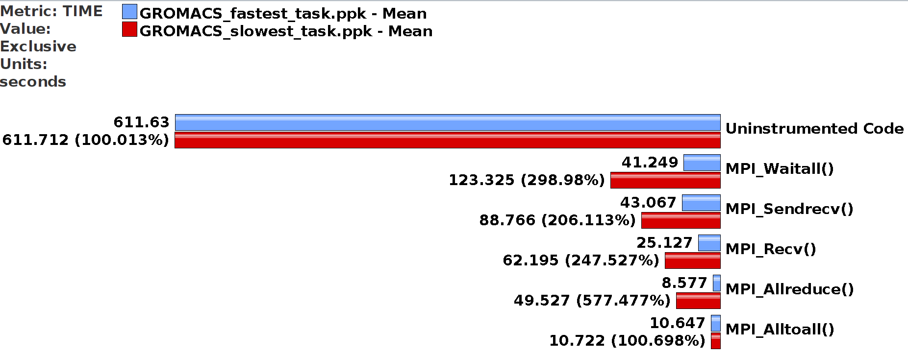
Figure 4: TAU Profiles for Fastest and Slowest Tasks

II-E Toggling Checkpoint and Parallel File I/O

With the insight gained from profiling tasks with min-max execution times, our focus turned to identify if the system factor was local to each node, or not, i.e., commonly present across multiple (or all) nodes. The network was previously ruled out as a contributor, leaving the parallel filesystem as the only candidate fitting the bill. Previous experiments enabled checkpointing at a frequency of once a minute, and each GROMACS task produced a 2 MB checkpoint file. Further, a deep dive into the GROMACS checkpoint code module revealed that MPI rank 0 was responsible for performing the file I/O after receiving data from other participating MPI ranks.

We set up an experiment to determine if disabling the checkpoint module would result in greater consistency in GROMACS execution time. Two 256-node ensemble workloads were simultaneously submitted, one with the checkpoint module enabled and the other with the checkpoint module disabled. To ensure that the tasks run for a sufficiently long time to allow the system factor a good chance to “show itself” during the execution, the number of simulation timesteps was set to 400,000. Figure 5 depicts the sorted task execution times of tasks in these two ensemble workloads. The orange line represents the ensemble workload where checkpointing was disabled, and the blue line represents the workload where checkpointing was enabled. Checkpointing is indeed correlated with the occurrence of the variation in task runtime.

Figure 5: Runtime Variation with Checkpoint Enabled/Disabled

Next, we identified the line in the checkpoint module representing the file write call. To identify the conditions necessary for the system factor to show up, we requested a 256-node batch job allocation and ran four 256-task ensemble workloads in the following configuration:

1. YY: Checkpoint enabled (Y) and file I/O enabled (Y); 2. YN: Checkpoint enabled (Y) and file I/O disabled (N); 3. NY: Checkpoint disabled (N) and file I/O enabled (Y); 4. NN: Checkpoint disabled (N) and file I/O disabled (N).

In Figure 6, tasks with IDs in the range 0-255 belong to configuration 1, tasks with IDs in the range 256-511 belong to configuration 2, tasks with IDs in the range 512-767 belong to configuration 3, and tasks with IDs in the range 768-1023 belong to configuration 4. System factors causing the runtime variation is triggered if checkpointing is enabled and the file I/O is enabled.

Figure 6: Toggling Checkpointing and File I/O

These results obtained from executing configuration 3 exonerate the parallel file system as the root cause for the variation. If the parallel file system was indeed the root cause, then the “diff” in the routine execution times (see Figure 4) between the fastest and the slowest tasks would have shown up in the write call. However, this is not the case — instead, the “diff” in the routine execution times shows up inside MPI routines. To further rule out the parallel file system as the cause, we set up an experiment involving the IOR synthetic parallel file I/O benchmark. The benchmark was configured to write 2 MB worth of “dummy” checkpoint data at a frequency of once every minute, thereby emulating the GROMACS checkpoint module. Identical copies of the IOR benchmark were executed inside an ensemble, and the ensemble workload was gradually scaled up from one to 256 KNL nodes on Theta. Regardless of the ensemble workload size, the IOR task performance remained virtually constant (i.e., no runtime variation was observed between the IOR tasks).

II-F Inducing Performance Variation

Assuming the system factor “shows up” uniformly for all applications, why is GROMACS affected while the IOR benchmark was not? The experimental observations thus far suggest that the MPI call structure surrounding the GROMACS checkpoint module makes it particularly sensitive to whatever system factor was responsible for causing the variation. We wondered if the “sensitivity” of the checkpoint module execution time to minor variations in the file write time can be triggered by replacing the write call with a sleep call for a “random” amount of time in the range of 0.09 to 0.25 seconds. These numbers were chosen based on the time to write a 2 MB checkpoint file.

We ran three successive sets of 256-node GROMACS ensembles within the same batch job. For Set 1, the checkpoint module and file I/O were enabled. For Set 2, the checkpoint module and file I/O were disabled, and for Set 3, the checkpoint module was enabled, but the file write call was replaced with a random sleep call. Figure 7 depicts the results of this experiment. Set 1 displays a moderate degree of variation in the task runtime while Set 2 displays a minimal degree of variation (expected). Surprisingly, Set 3, which replaces the file write call with an “equivalent” sleep call displays the highest degree of variation in task runtime. Specifically, the sleep call perturbed the execution of a few outlier tasks to the extent of adding hundreds of seconds to the total execution time.

Figure 7: Induced Performance Variation

II-G Relying on Prior Work

In summary, the observations from our experiments suggest that: 1. The system factor causing the variation is local to each KNL node (and task); 2. Its occurrence and the severity of the impact on task execution time can not be predicted but is bounded; 3. The system factor is not the result of faulty hardware; and 4. GROMACS performance is susceptible to the presence of this system factor when checkpointing is enabled.

The sleep call and the write call have a common “pathway” or element causing the behavior we seek to understand. Our collective hypothesis at this point was that the system factor is OS noise, but we did not know how to test this hypothesis. A brief review of the existing literature on prior performance variation studies yielded valuable insight. Chunduri et al. [12] report on the exogenous system factors known to cause performance variation on the Theta cluster. As part of their study, they investigated the impact of OS noise on the execution time of the Selfish benchmark [14] with and without “core specialization” — a mechanism allowing the user to dedicate a set of cores to execute OS services. They observed a ten-fold reduction in noise when core specialization was enabled. However, they did not explore the impact of OS noise on production HPC applications.

By default, core specialization on Theta is disabled, allowing the OS to select any core to schedule its services. We modified the GROMACS task configuration to execute on 63 KNL cores instead of using all the 64 cores, reserving one core on every node for the OS to schedule its services. Over several days, we executed ten 256-node ensemble workloads in this new configuration. Figure 8 depicts the results of employing a dedicated core for scheduling OS services — the range of GROMACS task execution time reduced from 16% (when using all 64 cores) to 3.5% (when using 63 cores). As a result of using one less CPU core, the individual task performance worsens by 1-2% but the collective performance of the workload improves.

Figure 8: Reserving a Dedicated Core for OS Services

III Discussion

Although we reduced task runtime variation putatively caused by OS noise, we still have no good way of proving through a set of measurements that the OS noise was indeed the dominant cause. By running all MPI processes of a GROMACS task on a single Theta node, network contention between the processes is minimized (all communication is through shared memory), ruling this out as a cause for the differential timings in the MPI routines. Is there another easily measured metric that might correlate to OS noise? The number of process context switches is a possible candidate, since it might suggest more direct OS activity, but it is more likely what happens between process context switch that matters rather than the number. We might try to measure the time spent in the OS, but there might be little variation, assuming the OS is doing similar tasks on each node. What is weird is that only a percentage of tasks are affected and the variation is showing up in MPI routines. This suggests that it matters where in the task’s execution the OS interference occurs, not how much time it lasts. We speculate that some of the GROMACS tasks are just unlucky and the OS interfers at times that disrupts MPI behavior, adding delays and impacting syncronication.

There is a need to fundamentally understand the genesis of performance variation resulting from exogenous and endogenous factors and study their impact on critical HPC applications such as GROMACS. Prior studies have been primarily conducted on (micro)benchmarks; it is largely unclear how these results translate to production HPC applications. Having some systematic means to perturb application execution might be useful to explore performance sensitivities. However, modeling the impact of task level performance variation on HPC ensembles is a different endeavor altogether. A more hierarchical methodology might be required: performance variation observed at a task level may, or may not, translate to performance variation at an ensemble workload level, especially if there are several more tasks to execute than available computing resources.

Before discussing performance reproducibility in ensemble computations, it is beneficial to reflect on performance variation assumptions of an HPC application. It is generally expected that a deterministic application code will exhibit minor, if any, relevant variation in its performance if it is run in the same configuration on the same machine. It is this expectation that forms the basis for HPC performance optimization where inefficiencies can be reliably identified and improvements made. That said, several exogenous factors can lead to performance variation, including differences in processor clock rates, contention with other running codes, operating system interference, and more. Endogenous to an application, there can be non-determinism inherent in its execution and fine sensitivities to memory and network operation.

Nevertheless, it is reasonable to maintain the expectation of minor performance variation in HPC applications; otherwise, our performance optimization methodology breaks down. It might be even assumed possible to characterize any variability within the context of the application code, in order to determine bounds and vulnerabilities. With this in mind, performance variation for an HPC application can be generally regarded as a distribution around expected performance value, one that very well might be able to be reproduced.

However, ensemble execution is a different matter. All factors for performance variation of a single HPC application are still valid for ensemble tasks. Instead of a single code, the variability analysis is compounded by the multiplicity of tasks. Indeed, tasks can interfere with each other as a result of sharing system infrastructure and cause perturbations that lead to further performance variation. In addition, it is essential to realize that how a task is configured at the time of its execution and the resources assigned are not necessarily fixed. The same task might be run in a variety of configurations during the lifetime of the ensemble computation. It is not the optimization of an individual task under a particular configuration that matters. Task performance naturally has a much fuller distribution because it covers a potentially broader set of options that the ensemble runtime system has to choose from during task scheduling.

A fundamental shift arising from ensemble (task) performance variability is that it is no longer the performance or optimization of a single task that is critical, but the collective performance of all ensemble members (viz., the makespan of the workload that matters). What implications does this have on performance reproducibility in ensemble computations? Are we asking for individual task performance to be reproducible, and by extrapolation, thinking the ensemble’s performance should then be reproducible? Given that an ensemble workflow maintains task dependencies, does this imply that reproducibility will require invariance in task execution ordering from one ensemble run to the next?

We contend that the focus of reproducibility should not be on whether an individual task’s performance is reproducible in ensemble computation. When a task is ready to run, it will then be scheduled and configured according to the resources allocated. If the task is run again at another point in the workflow, it might be configured differently and with different resources. It makes little sense to compare the two task executions if they are configured differently – a 4-node MPI+OpenMP task with 32 CPU threads per node will behave very differently from a 1-process instantiation of the task with 4 GPUs. Here performance variation stares the ensemble scheduler directly in the face. Furthermore, decisions regarding resource assignment might have less to do with optimal task performance than with dynamic resource availability and collective utilization of ensemble resources. Even as we relinquish the belief of single task performance reproducibility, we are constrained by need for collective performance invariance (viz., makespan) and reproducibility.

It is worthwhile to define three regimes of ensemble execution relative to resources and workload (tasks ready to run): (1) there are inadequate resources to run the entire workload, (2) there are adequate resources available to execute the workload, and (3) there are excessive (more than adequate) resources available to execute the workload. Understanding that the workload amount at any point in the ensemble computation will vary, without loss of generality, we can characterize the regimes. In (1), the appropriate and optimal subset of tasks will have to be selected and ordered to complete the workload. That decision is non-trivial and can involve other criteria than task performance per se. While tasks in a workload set are independent, some might be determined to be of higher priority. In (3), the correct subset of resources have to be selected, and the rest possibly released to save cost. In (2), the mapping of tasks to resources (which assumes alternative task configurations) has to be optimal. In all regimes, we are dealing with reasoning about the workload performance concerning the collective.

Even if we knew the expected performance of each task instance (for possible configurations and resource assignment), the scheduling problem is difficult a priori. Allowing for even a tiny variation in any task’s performance makes finding the “optimal” schedule significantly harder. A distribution of solutions will very likely be required. Knowing whether a task’s execution will be reproducible does little to make the problem tractable. If we forget about whether task performance is reproducible, how should we define “reproducibility” in the context of ensembles? One possible way to approach this is to simplify the focus of the problem of scheduling the next task. Indeed, given an executing subset of workload tasks, the ensemble runtime system must a) decide which task to execute next, b) select/allocate free resources to that task, and c) configure the task appropriately. Thus, the problem is reduced to deciding on the next task and its execution.

It is not to say that the problem is now easy. If we had any information about the performance of the remaining tasks, that might be beneficial, but we have to assume it will have performance variability. We may also need to consider non-stationary distributions from which individual task performance is drawn. Having no knowledge of expected performance is equivalent to high variability. Once a task begins, its performance is determined by its execution. The workload performance as a collective will be determined by the next task assignment, task by task. Interestingly, at those points extra information will be available about which task(s) finished and how resource availability may have changed as a result. Furthermore, it is possible to gain further information and insight into how well individual tasks are performing by employing support for observation and monitoring in the ensemble system.

In one sense, then, we could reason about ensemble reproducibility concerning whether the same decision would be made about scheduling the next task if the circumstances were the same in different ensemble executions, for every ensemble task. Unfortunately, this reasoning falls on its face since any task performance variation has the potential to make each ensemble execution different. If, instead, we recast reproducibility as making “locally optimal”scheduling decisions, there is more consistency across multiple runs of an ensemble computation that we can imagine.

Carrying this further, if we rationalize ensemble computing concerning its potential for massive makespan, we could imagine that its performance will begin to conform to the Law of Large Numbers. That is, the greater the “span” of tasks off the critical path, the less impact variations among those tasks will have acute effects, even if they are scheduled differently. That is rationally sound but likely difficult to actually prove experimentally. Lastly, although we have downplayed adaptability in this paper, the institution of an observation and monitoring framework would allow not only increased performance awareness to better inform future scheduling decisions, but also enable detection of performance anomalies when they arise, allowing corrective actions, however possible. The situational awareness of performance state coupled with in situ analytics and dynamic response to problematic behavior will make observation, monitoring, and adaptive control critical for harnessing reproducibility in ensemble computing.

This work was partially supported by the DOE HEP Center for Computational Excellence at Brookhaven National Laboratory under B&R KA2401045, as well as NSF-1931512 (RADICAL-Cybertools). We thank Andre Merzky and Li Tan for useful discussions and support.

References

- [1] S. Jha, S. Lathrop et al., “Incorporating Scientific Workflows in Computing Research Processes,” Computing in Science & Engineering, vol. 21, no. 4, pp. 4–6, 2019.
- [2] H. Lee, A. Merzky et al., “Scalable hpc and ai infrastructure for covid-19 therapeutics,” Platform for Advanced Scientific Computing Conference (PASC ’21), July 5–9, 2021, Geneva, Switzerland. ACM, New York, NY, USA, 2021, https://arxiv.org/abs/2010.10517.
- [3] A. Brace, I. Yakushin et al., “Coupling streaming ai and hpc ensembles to achieve 100–1000 faster biomolecular simulations,” in 2022 IEEE International Parallel and Distributed Processing Symposium (IPDPS). IEEE, 2022, pp. 806–816.
- [4] V. Balasubramanian, M. Turilli et al., “Harnessing the power of many: Extensible toolkit for scalable ensemble applications,” in International Parallel and Distributed Processing Symposium. IEEE, 2018, pp. 536–545.
- [5] P. M. Kasson and S. Jha, “Adaptive ensemble simulations of biomolecules,” Current Opinion in Structural Biology, vol. 52, pp. 87 – 94, 2018.
- [6] V. Balasubramanian, T. Jensen et al., “Adaptive ensemble biomolecular applications at scale,” SN Computer Science, vol. 1, no. 2, pp. 1–15, 2020, https://doi.org/10.1007/s42979-020-0081-1.
- [7] A. Merzky, M. Turilli, and S. Jha, “Raptor: Ravenous throughput computing,” in 2022 22nd International Symposium on Cluster, Cloud and Internet Computing (CCGrid), 2022, pp. 595–604.
- [8] L. Pouchard, S. Baldwin et al., “Computational reproducibility of scientific workflows at extreme scales,” The Int. Journal of High Performance Computing Applications, vol. 33, no. 5, pp. 763–776, 2019.
- [9] ——, “Use cases of computational reproducibility for scientific workflows at exascale,” arXiv preprint arXiv:1805.00967, 2018.
- [10] Y. Inadomi, T. Patki et al., “Analyzing and mitigating the impact of manufacturing variability in power-constrained supercomputing,” in SC’15: Proceedings of the International Conference for High Performance Computing, Networking, Storage & Analysis. IEEE, 2015, pp. 1–12.
- [11] A. Bhatele, K. Mohror et al., “There goes the neighborhood: performance degradation due to nearby jobs,” in SC’13: Proceedings of the International Conference on High Performance Computing, Networking, Storage and Analysis. IEEE, 2013, pp. 1–12.
- [12] S. Chunduri, K. Harms et al., “Run-to-run variability on xeon phi based cray xc systems,” in International Conference for High Performance Computing, Networking, Storage & Analysis, 2017, pp. 1–13.
- [13] S. Shende and A. Malony, “The TAU parallel performance system,” The International Journal of High Performance Computing Applications, vol. 20, no. 2, pp. 287–311, 2006.
- [14] P. Beckman, K. Iskra et al., “Benchmarking the effects of operating system interference on extreme-scale parallel machines,” Cluster Computing, vol. 11, no. 1, pp. 3–16, 2008.