scale=1,
color=black,
opacity=1.0,
angle=0,
contents=![[Uncaptioned image]](/html/2208.09047/assets/x1.png) \abstracttitleAbstract
\abstracttitleAbstract
Machine learning algorithms for three-dimensional mean-curvature computation in the level-set method
Abstract
We propose a data-driven mean-curvature solver for the level-set method. This work is the natural extension to of our two-dimensional error-correcting strategy presented in [Larios-Cárdenas and Gibou, DOI: 10.1007/s10915-022-01952-2 (October 2022)] [1] and the hybrid inference system of [Larios-Cárdenas and Gibou, DOI: 10.1016/j.jcp.2022.111291 (August 2022)] [2]. However, in contrast to [2, 1], which built resolution-dependent dictionaries of curvature neural networks, here we develop a single pair of neural models in , regardless of the mesh size. The core of our system comprises two feedforward neural networks. These models ingest preprocessed level-set, gradient, and curvature information to fix numerical mean-curvature approximations for selected nodes along the interface. To reduce the problem’s complexity, we have used the local Gaussian curvature to classify stencils and fit these networks separately to non-saddle (where ) and saddle (where ) input patterns. The Gaussian curvature is essential for enhancing generalization and simplifying neural network design. For example, non-saddle stencils are easier to handle because they exhibit a mean-curvature error distribution characterized by monotonicity and symmetry. While the latter has allowed us to train only on half the mean-curvature spectrum, the former has helped us blend the machine-learning-corrected output and the baseline estimation seamlessly around near-flat regions. On the other hand, the saddle-pattern error structure is less clear; thus, we have exploited no latent characteristics beyond what is known. Such a stencil distinction makes learning-tuple generation in quite involving. In this regard, we have trained our models on not only spherical but also sinusoidal and hyperbolic paraboloidal patches at various configurations. Our approach to building their data sets is systematic but gleans samples randomly while ensuring well-balancedness. Furthermore, we have resorted to standardization and dimensionality reduction as a preprocessing step and integrated layer-wise regularization to minimize outlying effects. In addition, our strategy leverages mean-curvature rotation and reflection invariance to improve stability and precision at inference time. The synergy among all these features has led to a performant mean-curvature solver that works for any grid resolution. Experiments with several interfaces confirm that our proposed system can yield more accurate mean-curvature estimations in the and norms than modern particle-based interface reconstruction and level-set schemes around under-resolved regions. Although there is ample room for improvement, this research already shows the potential of machine learning to remedy geometrical problems in well-established numerical methods. Our neural networks are available online at https://github.com/UCSB-CASL/Curvature_ECNet_3D.
keywords:
machine learning , mean curvature , Gaussian curvature , error neural modeling , neural networks , level-set methodMSC:
[2010]65D15 , 65D18 , 65N06 , 65N50 , 65Z05 , 68T201 Introduction
Curvature is a fundamental geometrical attribute related to minimal surfaces in differential geometry [3] and surface tension in physics [4, 5]. In particular, mean curvature plays a crucial role in solving free-boundary problems (FBP) [6, 7] with applications in multiphase flows [8, 9, 10, 11, 12, 13, 14], heat conduction and solidification [15, 16, 17, 18, 19], wildfire propagation [20], biological systems [21, 22, 23, 24], and computer graphics and vision [25, 26, 27, 28, 29, 30, 31]. In surface-tension modeling, for example, computing curvature accurately at the interface is essential for recovering specific equilibrium solutions to the FBP’s partial differential equations (PDE) [5]. Well-balanced numerical schemes that do so should also work appropriately near regions of topological change to avoid erroneous pressure jumps that may affect breakup and coalescence [21, 32, 33].
Over the years, the research community has devised several numerical procedures for solving FBPs efficiently. Among them, the level-set method [4, 34, 35] has emerged as a popular choice for its simplicity and ability to capture and transport deformable surfaces. The level-set framework belongs to the family of Eulerian formulations, alongside the phase-field [36] and volume-of-fluid (VOF) schemes [37]. Unlike Lagrangian front-tracking methods [38, 39], they all represent free boundaries implicitly with higher-dimensional functions. Thus, Eulerian formulations can handle complex topological changes naturally, with no need for overcomplicated interface-reconstruction (IR) algorithms [34].
The standard curvature-estimating method in the level-set framework is straightforward. Yet, level-set field irregularities often undermine its accuracy, especially around under-resolved regions and near discontinuities [21, 40, 32, 33]. To remedy these flaws, computational scientists have introduced different approaches. In [40], for example, du Chéné, Min, and Gibou have developed high-order reinitialization schemes that yield second-order accurate curvature computations on uniform and adaptive Cartesian grids. These schemes extend the idea of redistancing the level-set field with iterative algorithms until it resembles a signed distance function [8]. When executed correctly, not only can reinitialization restore level-set smoothness, but it can also dampen the critical problem of mass loss [41]. These efforts, however, do not always guarantee satisfactory results on coarse discretizations. And, although we can refine the mesh next to the free boundary with adaptive grids efficiently [42, 43], this only delays the onset of under-resolution issues. Moreover, there are FBPs, such as high- turbulent flows [44, 14], for which increasing the resolution in is prohibitive even on multicore computing systems. Here, we put forward a data-driven solution constructed on the above numerical schemes. Nevertheless, our goal is to attain high mean-curvature precision around under-resolved regions while short-cutting the need for further mesh refinement.
Other practitioners have adopted a geometrical approach to reduce mean-curvature errors when handling level-set discontinuities. Among them, we can find the schemes of Macklin and Lowengrub [21]. They have approximated two-dimensional interfaces with least-squares quadratic polynomials and recalculated curvature on local sub-grids near level-set singularities (i.e., around kinks in the underlying level-set function emerging from free-boundary collisions). Similarly, Lervåg [32] has devised a method to parametrize interfaces with Hermite splines and estimate curvature, spawning no additional sub-cell stencils. While accurate, these systems are difficult to extend to three-dimensional space because of their surface reconstruction requirement. However, their topology-aware strategy has motivated the emergence of sophisticated yet easy-to-integrate non-curve-fitting alternatives derived from insertion/extraction algorithms [45]. In this context, technologies, such as the local level-set extraction method (LOLEX) [33], have recently outperformed any of their predecessors when computing geometrical attributes in extreme interfacial conditions (e.g., involving self-folding bodies). In the same spirit as LOLEX, here, we have designed a mean-curvature solver that researchers can readily incorporate into existing level-set codebases. Its inner workings are optimized to leverage distance and other geometrical information to model and fix errors in finite-difference-based mean-curvature estimations.
In this manuscript, we propose to address the level-set’s curvature shortcomings from a data-driven perspective. The latest developments of Qi et al. [46] and Patel et al. [47], in particular, have inspired our machine- and deep-learning incursions for solving not only for mean-curvature [48, 2, 1] but also passive transport [49]. In the pioneering study of Qi et al. [46], the researchers fitted two-layered perceptrons to circular-interface samples to estimate curvature from area fractions in the VOF representation. Later, in [47], Patel et al. extended this idea and trained mean-curvature feedforward networks with randomized spherical patches in three-dimensional VOF problems. In both cases, their approaches showed promising, accurate results in two-phase flow simulations. Like these, there have been other contemporary deep learning implementations devoted to solving geometrical difficulties in conventional numerical schemes. These include, for instance, the curvature prediction from angular and normal-vector information [50] in front-tracking and the neural calculation of linear piecewise interface construction (PLIC [51]) coefficients [52] in the VOF method. Likewise, one can find advancements in the level-set framework, such as Buhendwa, Bezgin, and Adams’ consistent algorithms for inferring area fractions and apertures for IR [53].
Our research incorporates the notion of neural error quantification first introduced in computational fluid dynamics to fix artificial numerical diffusion and augment coarse-grid simulations [44, 49]. More importantly, our study is the natural extension to of the preliminary two-dimensional error-correcting strategy presented in [1]. In previous work, we optimized simple multilayer perceptrons (MLP) [54] with samples from circular and sinusoidal zero-isocontours to offset numerical curvature errors at the interface. Then, we blended the neurally corrected and the baseline approximations selectively to improve precision around under-resolved regions and near steep111In this work, we use the term steep to qualify a surface with regions where the dimensionless mean curvature is much greater than 0.1. interface transitions. Compared to a network-only approach [48] and an earlier hybrid inference system [2], error correction has proven more effective at closing the gap between the expected curvature and its numerical estimation. Indeed, beyond-usual contextual information (e.g., level-set values, gradients, and the curvature itself), dimensionality reduction, and regularization have been important factors in achieving the results reported in [1].
Here, we propose a hybrid solver to estimate mean-curvature in three-dimensional free-boundary problems. At the core of our system, we have two shallow feedforward neural networks. These models ingest preprocessed level-set, normal-vector, and curvature information to fix numerical mean-curvature approximations selectively along the interface. To reduce the problem’s complexity, we have used the local Gaussian curvature [3], , as an inexpensive stencil classifier and fitted these networks separately to non-saddle (where ) and saddle (where ) input patterns. Unlike [47], Gaussian curvature is essential in our strategy for enhancing generalization and simplifying neural architecture and design. Non-saddle stencils, for example, are easier to handle because they exhibit a mean-curvature error distribution characterized by monotonicity and symmetry. While the latter has allowed us to train only on half the mean-curvature spectrum, the former has helped us blend the machine-learning-corrected output and the baseline estimation seamlessly around near-flat regions. On the other hand, the saddle-pattern error structure is less clear; thus, we have exploited no latent characteristics beyond what is known. Such a distinction between stencils makes learning-tuple generation in more involving than its planar counterpart [1]. In this regard, we have trained our models on not only spherical but also sinusoidal and hyperbolic paraboloidal patches at various configurations. Our approach to building their corresponding data sets is systematic but gleans samples in a randomized fashion while ensuring well-balancedness as much as possible. In the same spirit as [49, 1], we have resorted to standardization and dimensionality reduction as a preprocessing step and integrated layer-wise regularization to minimize outlying effects. In addition, our strategy leverages mean-curvature rotation and reflection invariance, as in [53], to improve stability and precision at inference time. The synergy among all these features has led to a performant mean-curvature solver that works for any grid resolution. And there is more to it. Experiments with several geometries have confirmed that our proposed system yields more accurate mean-curvature estimations in the and norms than modern particle-based IR [13] and level-set schemes around under-resolved regions. Although there is ample room for improvement, this research already shows the potential of machine learning and neural networks to remedy geometrical problems in well-established numerical methods. Our results below and those given in preliminary studies [44, 53, 49, 1] suggest that data-driven solutions perform better when they supplement conventional frameworks rather than when they try to replace them.
We have organized the contents of this manuscript into five sections. First, Sections 2 and 3 summarize the level-set method and adaptive Cartesian grids, which are the only way of handling FBPs in efficiently. Then, Section 4 describes all the aspects related to our proposed hybrid inference system and the algorithms to generate its learning data and deploy its components. After that, we evaluate our strategy through a series of experiments in Section 5. Finally, we reflect on our findings and outline some future work in Section 6.
2 The level-set method
The level-set method [4] is an implicit formulation for capturing and evolving interfaces represented as the zero-isocontour of a high-dimensional, Lipschitz relation known as the level-set function. In this framework, we denote an interface by , which partitions the computational domain into and 222For compactness, we will omit functional dependence on time in the rest of this paper.. Deforming and convecting in level-set schemes require solving a Hamilton–Jacobi PDE known as the level-set equation,
| (1) |
where is an application-dependent velocity field. Traditionally, we solve eq. 1 with high-order accurate schemes, such as HJ-WENO [55], or with unconditionally stable semi-Lagrangian approaches [56, 57, 42] in passive-transport FBPs.
The implicit nature of the level-set framework makes it straightforward to calculate normal vectors and mean curvature values at virtually any point . We define both attributes with
| (3a) | ||||
| (3b) | ||||
Likewise, one can compute the Gaussian curvature at any using Goldman’s derivation [59] and the extended relation for implicit surfaces provided by [58] as
| (4a) | ||||
| (4b) | ||||
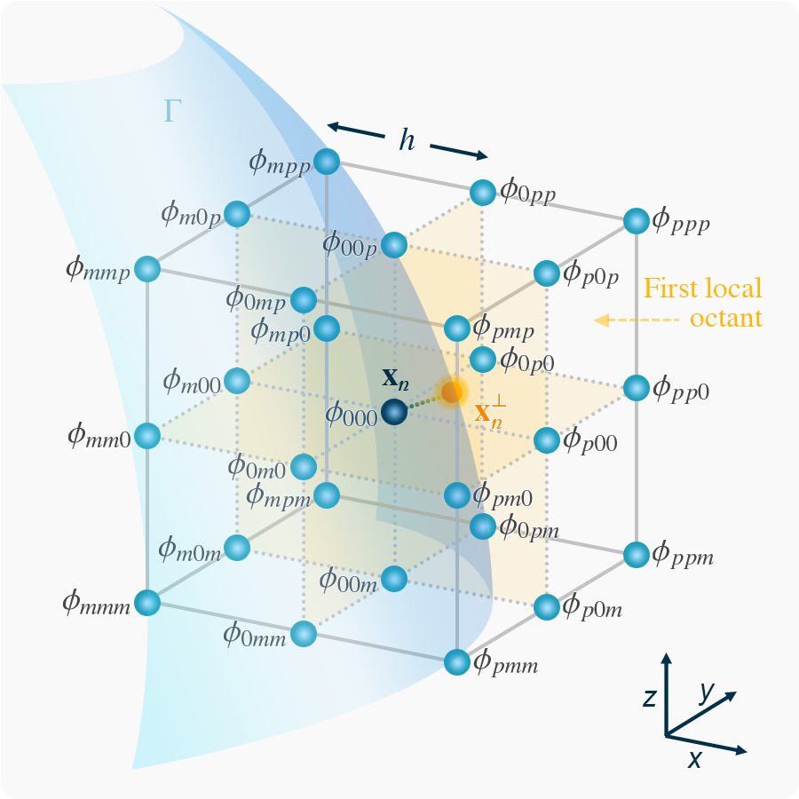
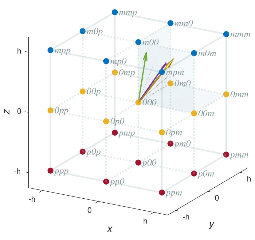
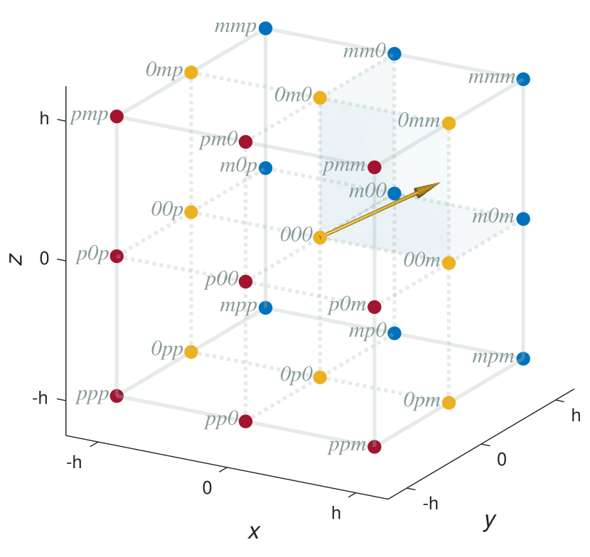
where is the adjoint of ’s Hessian matrix. In practice, we employ stencils of level-set values (see fig. 1) and first- and second-order central differences to discretize eqs. 3 and 4b and approximate the gradient in eq. 2 [60, 40]. Equation 4b is critical for our current research since it allows us to characterize grid points333We use the terms grid point and node interchangeably to refer to the discrete locations in a Eulerian mesh. for downstream regression.
| (5) |
where and are the principal curvatures [3].
Curvature computations in the level-set representation are often noisy because of the second derivatives in eqs. 3 and 4b. However, it is possible to estimate and accurately if guarantees sufficient smoothness and regularity [40]. On this point, signed-distance functions are an excellent choice because they are beneficial not only for curvature calculations but also for mass preservation. Unfortunately, even if one chooses as a signed-distance function at the onset, we cannot ensure that solving eq. 1 under an arbitrary velocity field will preserve this feature throughout the simulation. For this reason, it is typical to redistance periodically by solving the pseudo-transient reinitialization equation [8]
| (6) |
to a steady state (e.g., for iterations) using a Godunov spatial discretization and high-order temporal TVD Runge–Kutta schemes [61, 62]. In eq. 6, represents fictitious time, is a smoothed-out signum function, and is the arbitrary level-set function before the reshaping process. Furthermore, when resembles a signed-distance function, , several calculations simplify, and one can produce more robust estimates of eqs. 2 to 4 [40]. Similarly, preliminary research [48, 2, 1] has shown that redistancing can help remove unstructured patterns that may undermine the performance of deep learning curvature models in .
In this study, we have resorted to the level-set algorithms developed by Du Chéné, Min, and Gibou [60] and their parallel implementation on p4est [63], as described in [43]. For a more comprehensive analysis, we refer the interested reader to the level-set texts by Osher, Fedkiw, and Sethian [64, 34] and the recent review by Gibou et al. [35].
3 Adaptive Cartesian grids
Solving FBPs on uniform grids is particularly expensive when the underlying phenomena exhibit a wide range of length scales. High- channel-flow simulations [14], for example, require a high grid resolution along the boundary layers to capture wake vortices and other flow characteristics. In such cases, working with adaptive Cartesian grids is more cost-effective because we only refine the mesh next to , where accuracy is needed the most [42].
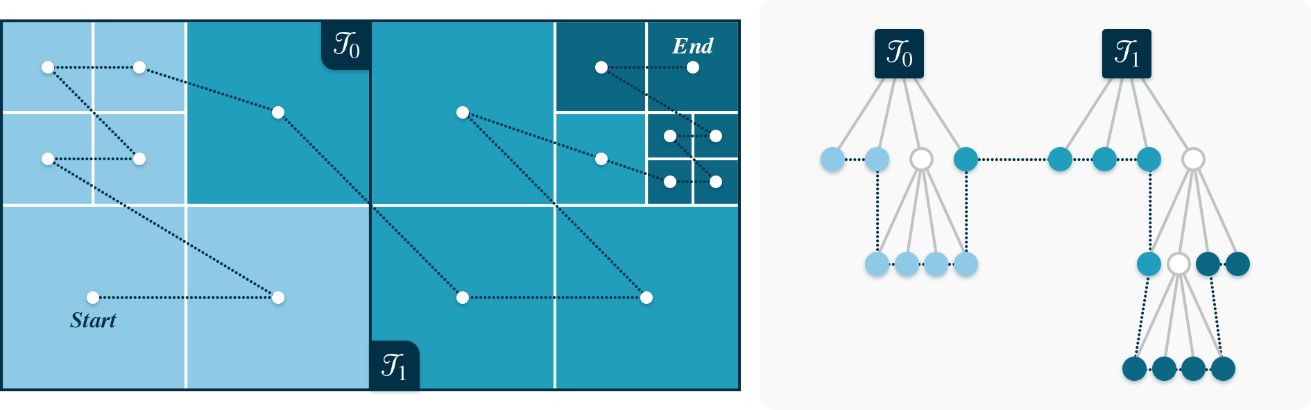
In this context, quadtree- () and octree-based () Cartesian grids have grown popular among level-set practitioners because they are easy to implement with signed distance functions [42, 60, 43]. Quad/octrees are rooted data structures covering a region . They are composed of cells organized recursively into levels, where each cell either has four (eight) children (i.e., quadrants (octants)) or is a leaf [65]. Once constructed, a quad/octree with maximum depth can support several operations efficiently, such as searching in and sorting [42]. Figure 2 illustrates two squared quadtrees, where and have and maximum levels of refinement. Figure 2 also describes a straightforward characterization of a domain’s discretization in from the p4est library’s perspective.
The p4est framework [63] is a family of parallel algorithms for grid management. This library provides scalable methods for parallelizing, partitioning, and load-balancing spatial tree data structures across heterogeneous computing systems. Recently, p4est has been shown to handle up to 458,752 cores [66] in various resource-intensive tasks where working with the memory and processing power of a single computing node is unfeasible (e.g., see [14]). In p4est, we build an adaptive Cartesian grid with non-overlapping trees rooted in a coarse scaffolding known as the macromesh. This coarse grid can adopt different configurations, but we always assume it to be small enough to be replicated on every process. For simplicity, here, we have limited ourselves to uniform brick-like macromesh layouts, as depicted on the left diagram of fig. 2.
Each tree in a p4est macromesh first undergoes coarsening and refinement based, for instance, on the interface’s location. In this study, we have opted for Min’s extension [67] to the Whitney decomposition criteria [42], as presented in [60, 43], to guide the discretization process. In particular, we mark a cell for refinement if the criterion
| (7) |
holds, where is a cell vertex (i.e., a grid node), is ’s Lipschitz constant (set to across ), and is ’s diagonal. Conversely, we tag a cell for coarsening if the condition
| (8) |
is valid. Besides these criteria, we can enforce a uniform band of smallest cells around by subdividing quadrants (octants) for which the inequality
| (9) |
is true. Our research considers only cubic cells to reduce the number of degrees of freedom in the problem at hand. Hence, in eq. 9 (see fig. 1), where is ’s mesh size, and is the maximum depth of the unit-hexahedron octrees in .
After fitting to using eqs. 7 to 9, p4est linearizes the trees using a -curve that traverses their leaf cells, as shown in fig. 2. Such a space-filling curve [68] helps partition and load-balance among processes while ensuring that leaves with close -indices remain close to each other, on average. In practice, this property is beneficial because it reduces MPI communications [69] and leads to efficient interpolation and finite difference procedures [43]. For additional p4est details and algorithms, the reader may consult [63].
As remarked at the end of Section 2, the present study is also based on Mirzadeh and coauthors’ parallel level-set schemes [43]. Mirzadeh et al. have exploited p4est’s global-indexing and ghost-layering features to devise a simple reinitialization procedure and a scalable interpolation algorithm for semi-Lagrangian advection. In the upcoming sections, we will use their redistancing scheme and Algorithm 2 to solve eq. 6 and estimate at . Meanwhile, we refer the reader to [43, 42, 60] for further information about parallelizable level-set procedures on non-uniform meshes.
4 Methodology
In this study, we investigate the possibility of extending the error-correcting approach introduced in [49, 1] to the three-dimensional mean-curvature problem. Our goal is to endow the level-set framework with data-driven mechanisms that compensate for its lack of inbuilt features to calculate at the interface [5]. Traditionally, one circumvents this limitation by first evaluating eq. 3b at the grid nodes. Then, we interpolate these results at their nearest locations on . This procedure, however, does not always yield accurate estimations around under-resolved regions and steep surface portions. For this reason, we propose a methodology that computes on-the-fly corrections to such numerical approximations using deep learning. More succinctly, if represents the dimensionless mean curvature444A few notation pointers: denotes the numerical baseline estimation to the dimensionless mean curvature, is the neurally corrected value, and is the best approximation from our proposed hybrid solver to the true . interpolated at node ’s perpendicular projection
| (10) |
then the expression
| (11) |
realizes the numerical deviation from the true by some .
We claim neural networks trained on various stencil configurations can model and fix selectively. Here, we plan to devise a hybrid curvature solver by coupling these networks and the schemes from Section 2 to furnish better estimations denoted by . In particular, one should restrict such an inference system to interface nodes, where holds at least for one of the six neighbors at , in the direction of the standard basis vectors .
4.1 A hybrid mean-curvature solver enhanced by error-correcting neural networks
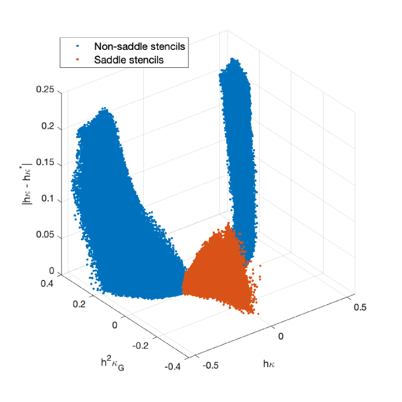
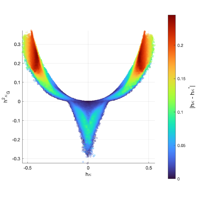
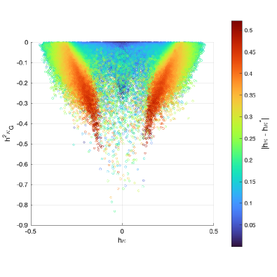
In analogy to the two-dimensional problem in [1], we propose using a neural function, , to characterize in eq. 11. However, building this neural network requires further analysis in than simply deciding on what features it should ingest. For example, fig. 3 plots the distribution of for a collection of nodes adjacent to randomized sinusoidal surfaces. Sinusoidal waves are essential because they host a variety of stencil patterns determined by a wide range of Gaussian curvature values associated with their center nodes. Section 4.2.2 discusses this class of interfaces from the training point of view, but we introduce them at this point to motivate neural network design. Let and be the linearly interpolated, non-dimensionalized mean and Gaussian curvatures at . Then, a swift inspection of fig. 3 reveals the following key observations:
-
OB.1
If , we have that as , and we can safely disregard .
-
OB.2
If , grows nonlinearly with and in a less separable fashion.
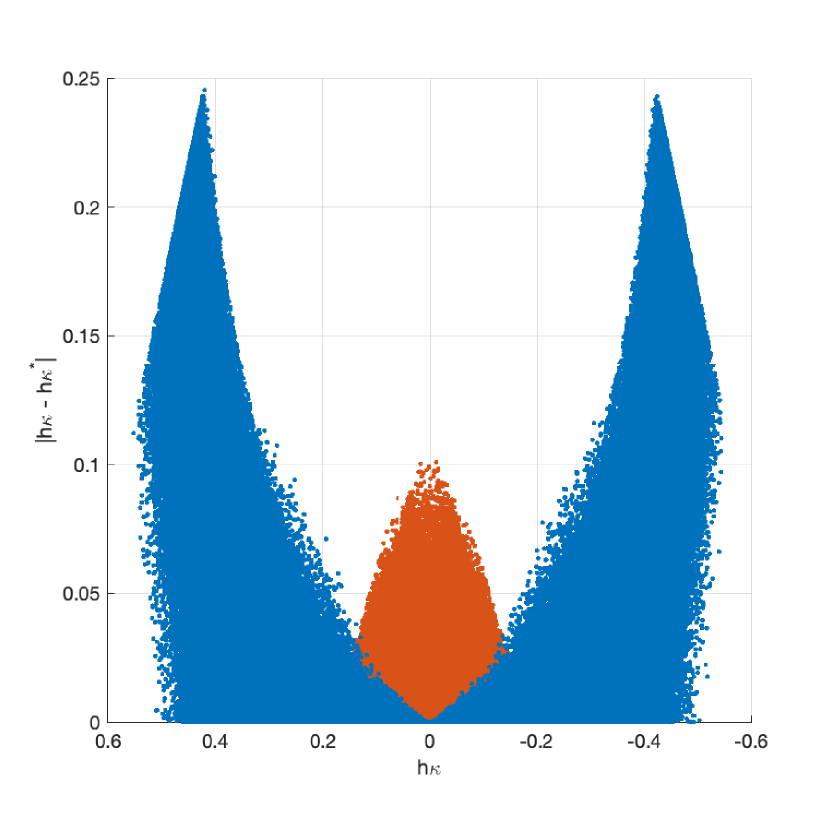
These observations suggest incorporating as an inexpensive stencil classifier. In particular, OB.1 corresponds to the typical behavior alluded to in [2, 1] for the two-dimensional curvature problem. Here, we refer to patterns described by this observation as non-saddle stencils. As seen in figs. 3(b) and 3(c), there is an intrinsic symmetry about the plane that we can exploit to simplify ’s topology. In this case, we can train only on the negative mean-curvature spectrum and rely on numerical schemes to determine whether the stencil belongs to a convex or concave region.
Observation OB.2, on the other hand, depicts a more complex use case that prevents us from exploiting symmetry like before. For instance, can be large, even for saddle stencils555We will extend the usage of the non-saddle and saddle qualifiers to distinguish not only stencils but also patterns, regions, samples, and data—all of them characterized by observations OB.1 and OB.2. whose value at is close to zero (e.g., see fig. 3(c)). This non-saddle- and saddle-pattern dichotomy prompts us to build two neural functions: and . At inference time, the solver would choose one or the other depending on . To distinguish non-saddle from saddle objects, sets, or artifacts, we will continue to use the superscripts and in the remaining sections of this manuscript.
and are as simple as MLPs. Figure 4 overviews their distinctive cascading architecture organized into five hidden layers. This diagram also illustrates the preprocessing module and a skip-connection that carries the signal from the input layer to a non-adaptable output neuron. The latter completes the error-correcting task by adding to the value computed internally to produce . As stated above, we expect to be closer to than , especially around under-resolved regions.
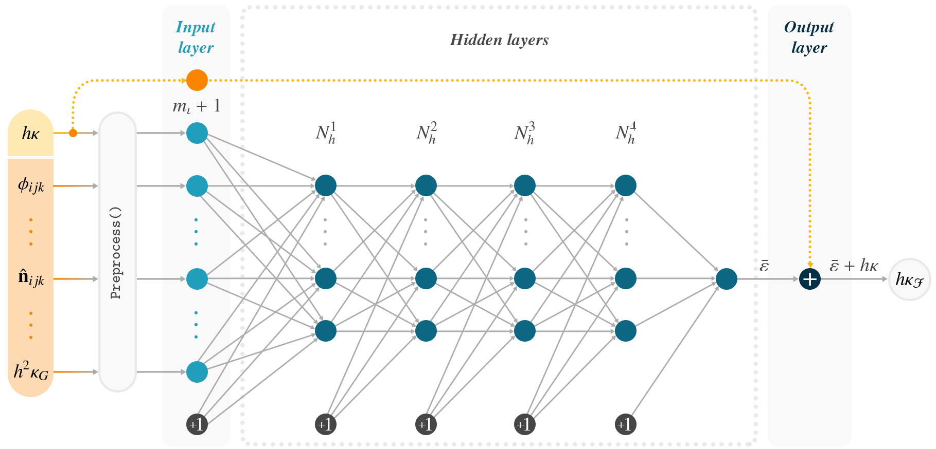
The Preprocess() subroutine in fig. 4 transforms incoming raw feature vectors into a more suitable representation for training and evaluating our downstream regressor [70]. In this work, we have constrained ourselves to evaluate data extracted only from regular -uniform 27-point stencils. Later, in Section 4.3, we will discuss the Preprocess() module’s specific implementation alongside the technical corners of the project. To provide and with as much information as possible, we consider more field data than just level-set values [48, 2] (or volume fractions in VOF technologies [46, 47]). Similar to the two-dimensional approach [1], our hybrid solver and models take in stencil level-set and gradient data, as well as the Gaussian and mean curvatures projected onto from the center grid point (see fig. 1). We have organized all these features into data packets of the form
| (12) |
where , with 666This notation resembles the Pythonic representation of a dict data type. We also use , , and as subscripts to enumerate grid points in a stencil., is a nodal attribute within ’s stencil centered at .
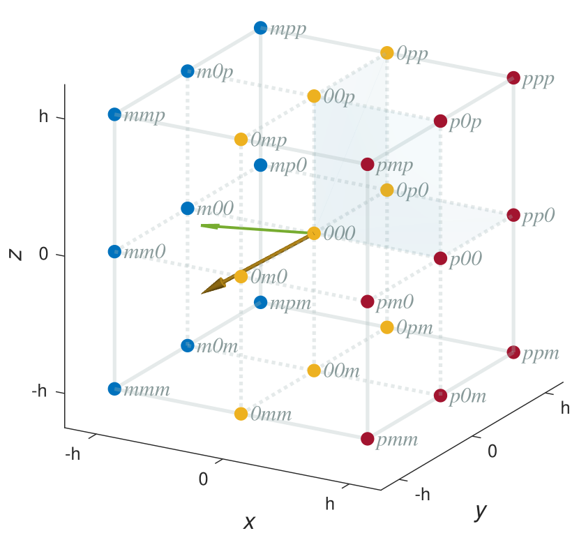
Likewise, we exploit curvature rotation and reflection invariance to reduce the problem’s degrees of freedom and improve prediction stability in two ways. First, we train and with a single class of normalized stencil configuration. In particular, we can always find a sequence of 90-degree rotations about the Cartesian-coordinate axes to leave into its first standard form, , where has all its components nonnegative. Not only does rotating stencils in this manner preserve and , but it also prevents our MLPs from diverting neural capacity to unnecessary data-packet orientations. This type of normalization is a staple preprocessing step in eigenface computation [71, 72]. And recently, it has been incorporated into data-driven semi-Lagrangian advection [49] and two-dimensional curvature estimation [1]. Figures 5(a) to 5(c) exemplify the reorientation process on the raw data packet, , associated with an arbitrary interface node . The reader may track ’s transformation into by following the evolution of its nodal labels and colors.
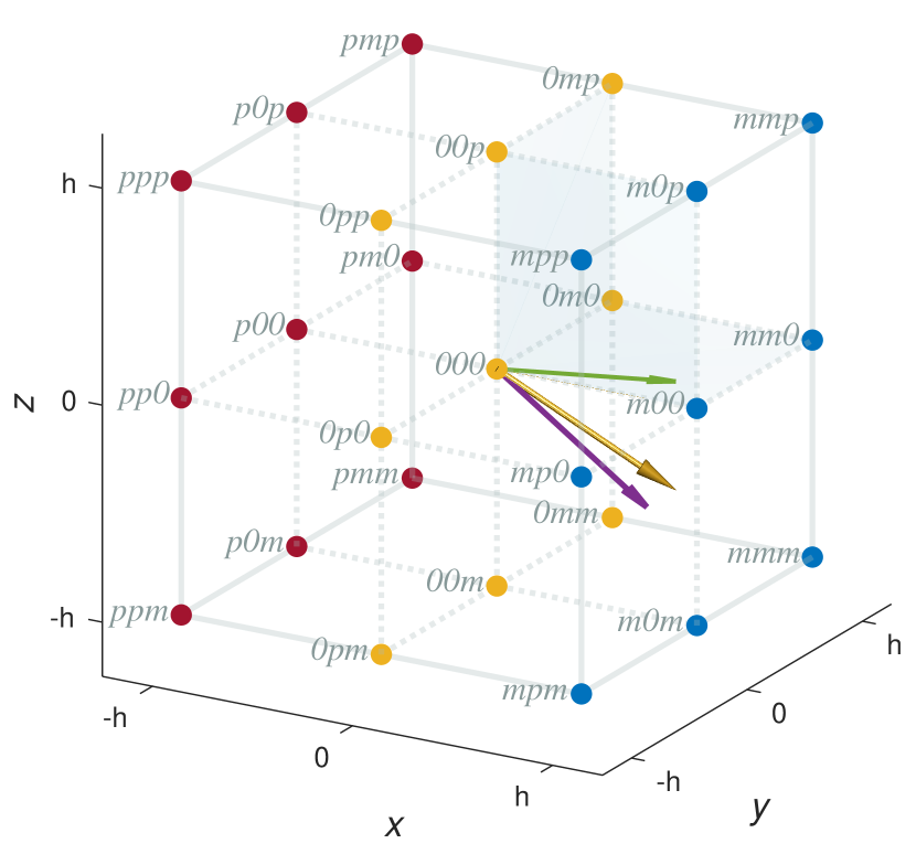
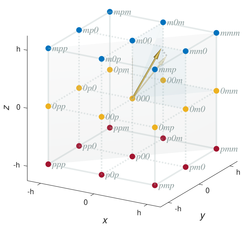
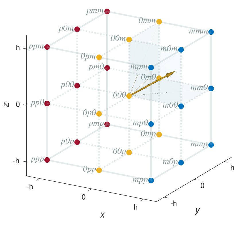
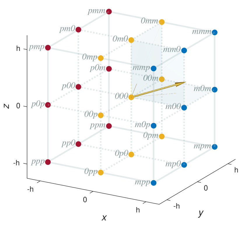
The second way of leveraging curvature rotation and reflection invariance regards symmetry enforcement. Practitioners have already used this resource to estimate volume fractions and apertures [53] and improve two-dimensional curvature accuracy in level-set [1] and VOF [73] schemes. The idea is to reflect and rotate a standard-formed data packet to extract additional stencil variations while keeping ’s components nonnegative. The benefit of such a process is twofold. At the inference stage, we can evaluate our MLPs on these data packets and take the average of the corrected curvature predictions. During training, this procedure facilitates data augmentation because it provides a geometric means for producing multiple samples per interface node. Figures 5(c) to 6 depict ’s six standard forms. Each corresponds to a permutation of the reoriented unit normal-vector entries at the center grid point of fig. 5(c). To get these variations, we have combined a sequence of reflections about the planes and and rotations about the Cartesian-coordinate axes, as shown in Algorithm 1.

We now introduce our hybrid mean-curvature solver, which yields for an interface node with a complete, -uniform stencil. The listing, shown in Algorithm 2, integrates traditional numerical schemes with the machine learning ingredients we got acquainted with above. This routine assumes that we have already fitted and to their respective training sets, as described in Section 4.2. In the same manner, it expects precomputed nodal level-set values and unit normal vectors ,777We distinguish -element vectors from 3-by- matrices by using bold lowercase symbols (e.g., ) and normal-weight uppercase letters (e.g., ). Here, denotes the number of grid points in . We have realized these abstractions using ghosted, parallel PETSc [74] vectors in p4est [63]. evaluated at least on a uniform band of half-width around (see eq. 9). Our hybrid solver also requires and to be extracted from a reinitialized level-set field that resembles a signed distance function. Other formal parameters include the mesh size and the and bounds for blending non-saddle averaged predictions with their numerical approximations near zero. Similarly, we need the dimensionless Gaussian curvature lower bound to discriminate non-saddle from saddle data packets.
Algorithm 2 is straightforward. In the beginning, we compute ’s numerical mean and Gaussian curvatures using finite-difference schemes to discretize eqs. 4b and 3b [40]. Then, we resort to linear interpolation to estimate and at [43]. represents the baseline we want to improve, and the next course of action depends on whether belongs to a non-saddle or saddle region. We resolve this classification subproblem by verifying if exceeds , which we have set throughout this study to (see OB.1 and OB.2). This threshold has resulted from examining various data sets, like those in fig. 3 and Section 4.2.3. In such analyses, we have observed that remains bounded by , even for interface grid points where . This finding has allowed us to slide the non-saddle/saddle decision boundary and extend our symmetrized approach to improve accuracy near .
If belongs to a non-saddle region, we can terminate Algorithm 2 prematurely whenever drops below . This threshold accounts for the ability of traditional numerical schemes to perform well along flat interface sectors. Here, is also equivalent to the learning hyperparameter , which we have chosen in analogy to the two-dimensional curvature problem [1]. Next, we select or , depending on the pattern type. For succinctness, MLCurvature() references to the appropriate MLP through the alias, which processes a transformed version of ’s data packet . To assemble , we employ the CollectFeatures() module, which reads in and structures field data, as provided in eq. 12. Then, we generate its six standard forms (see figs. 5(c) to 6) with Algorithm 1 while taking special care of the exclusive negative-mean-curvature normalization for non-saddle stencils.
The last portion of Algorithm 2 carries out inference and symmetry enforcement. In the former task, we evaluate on ’s preprocessed standard forms and average the corresponding corrected mean curvatures into . Afterward, MLCurvature() finishes as soon as we find for saddle stencils. Non-saddle regions, on the other hand, require some post-processing before outputting . To improve non-saddle accuracy and prevent sharp transitions near zero, we blend and linearly for , where . Finally, we restore the expected mean-curvature sign from and exit Algorithm 2 by returning to the calling routine.
The following subsections describe our methodology to assemble and —the training sets for and . Also, we provide implementation details to train, instantiate and deploy our MLPs to numerical applications.
4.2 Training
Although generating training data sets for our MLPs is an expensive endeavor, one must carry out this task just once. The idea is to construct and by following randomized strategies that guarantee well-balanced distributions.
Our data-generating approach extends the algorithms described in [1, 47] to three-dimensional level-set schemes. In [1], we developed a systematic yet scalable framework based on non-dimensionalizing the curvature-inference problem. Once more, we have adopted that methodology to confine and to (absolute) dimensionless mean curvatures between and ,888It is recommended to enforce to improve ’s interpolative power near the upper end of the negative mean-curvature spectrum. For us, and are equivalent. where for saddle data packets (see fig. 3). Together, non-dimensionalization and preprocessing have made it possible to train a single pair of MLPs on one mesh size and port the optimized models across resolutions with marginal accuracy variations.
Next, we examine three kinds of training surfaces to build and . First, we consider spherical patches to extract non-saddle learning tuples, similar to [47]. Likewise, in analogy to [1], we use three-dimensional sinusoidal waves to capture a wider diversity of patterns and enrich the contents of . As noticed above, sinusoids can produce saddle stencils, and here we incorporate a subset of those samples into . Then, we evaluate hyperbolic paraboloids as the third class of training surfaces. In particular, hyperbolic paraboloids are to as spheres are to . These saddle interfaces are necessary because it is more difficult and costly to determine the correct sinusoidal parameters to populate on the entire interval for .
4.2.1 Spherical-interface data-set construction
Spheres are our first kind of elementary learning surface. We have chosen them because it is trivial to calculate their exact mean curvature as , where is their nonzero radius. Also, it is easy to compute normal distances to spheres, and it is straightforward to integrate them into level-set applications as splitting criteria (see eqs. 7 to 9). Formally, the level-set field
| (13) |
defines a signed distance function with a spherical interface centered at , where for all points on . The latter statement makes spheres the surface of choice to populate in our training pipeline.
We have adapted the procedure to collect spherical training samples from the strategy suggested by Patel et al. [47]. In their research, the authors proposed to generate thousands of spheres with uniformly distributed random radii and extracted a single learning tuple from each at a random surface location. We have modified those heuristics in two fundamental ways. The first difference lies in how we space out when defining . In this regard, we draw radii from randomly distributed mean curvatures instead of retrieving from uniformly distributed radii. Also, we produce more than one learning sample from each while enforcing our problem-simplifying negative-mean-curvature normalization. Algorithm 3 combines these steps into a routine to build —the set of spherical-interface learning pairs. Ultimately, will take in alongside complementary data from the sinusoidal geometries discussed in Section 4.2.2.
The list of formal parameters for Algorithm 3 includes the maximum level of refinement, , and the nonnegative target dimensionless mean-curvature bounds, and . In our case, we have chosen and across grid resolutions to non-dimensionalize the non-saddle portion of the problem. Similarly, we have selected as the maximal because it is equivalent to the dimensionless mean curvature associated with the smallest resolvable sphere of radius . In the same manner, we provide Algorithm 3 with the number of distinct spheres to evaluate and how many samples we desire from each patch. Here, we have chosen and to populate with two million learning pairs. At last, we supply and : the number of redistancing steps and the amount of random uniform noise. Later, we will employ these to alter the otherwise exact signed distance function in eq. 13.
First, Algorithm 3 solves for and the target curvature bounds. Then, it uses these to populate the array TgtK with NSph decreasing uniform random steps between and .
For each , we define its radius and use it to spawn a level-set field, , whose spherical interface centers randomly at . Then, we find a couple of random (spherical-coordinated) angles, and , to locate a point on . The computation of and replicates the techniques suggested by Patel et al. [47], who showed that the stochastic nature of these azimuthal and polar angles guarantees a uniform sampling coverage of the spherical surface. allows us to create a -side-length bounding box centered at , where rounds each component to the nearest multiple of . Afterward, we use and to discretize with an adaptive Cartesian grid that ensures a uniform band of half-width around . Such a small bounding box helps cut down processing costs in , especially as . Later, we will reap the benefits of minimal bounding boxes as we transition to interfaces with no analytical distance-to-point formulae.
The following statements in Algorithm 3 evaluate eq. 13 on and gather its nodal level-set values into the vector . The latter contains exact signed distances, which we perturb in two ways to favor generalization. First, we alter by adding uniform noise, as in , where . Then, we reinitialize by solving eq. 6 with iterations, as in [2, 1]. Shortly after redistancing, we employ to estimate nodal unit normal vectors, , and baseline curvatures, and , to prepare data collection.
A loop traversing the set of extracted interface nodes with regular, -uniform stencils orchestrates the data collection subtask. The traversal pattern is typical not only for data-generative routines but also for testing and deploying Algorithm 2. Essentially, for each node , we start by structuring its features into a data packet containing the (linearly) interpolated, non-dimensionalized curvatures at (see eq. 12). Then, we normalize so that whenever the stencil belongs to a convex region and . Furthermore, as remarked in Section 4.1, any interface grid point can give rise to six standard-formed data packets through Algorithm 1 (see figs. 5(c) to 6). Hence, one must generate a tuple for every variation , having all different input patterns map to the same output. In Algorithm 3, these tuples are accumulated in the auxiliary set . And, eventually, we pull NSamPerSph random samples from it and add them to . Algorithm 3 thus completes after exhausting the entries in TgtK. Upon exiting, the calling routine receives with learning samples that exhibit a well-balanced frequency distribution on the -axis.
4.2.2 Sinusoidal-interface data-set construction
Three-dimensional sinusoidal waves are our second type of elementary surface. They are the analog to the planar sinusoids first considered in [2]. Unlike spherical patches [47], sinusoidal waves are critical for training and because we can use them to extract non-saddle and saddle samples, as seen in fig. 3.
To better organize the generative process, we have chosen two separate data sets, and , which prevent mixing non-saddle and saddle patterns. Their learning tuples originate from level-set functions characterized by sinusoidal interfaces. These waves embedded in are parametrized as Monge patches [3] of the form
| (14) |
where denotes the amplitude, and and are the frequencies in the and directions. Expressing a sinusoidal surface in this manner allows us to calculate the exact mean and Gaussian curvatures for any with
| (15) |
where and .
Given a sinusoid in its canonical frame (i.e., as provided in eq. 14), we can construct the level-set function
| (16) |
where yields the shortest distance between a point and a surface. This definition of partitions the computational domain so that lies strictly above , and is found right beneath it.
The procedure to populate and requires fiddling with , , and to gather an assortment of learning tuples. However, additional pattern variations are possible if one introduces affine transformations [75] to perturb the canonical patch in eq. 14. In this work, we have constrained ourselves to rotating and translating the local coordinate system, , that holds . More specifically, if is the translation induced by a shift vector , and is the rotation by an angle about some unit axis , then
| (17) |
maps points and vectors in homogeneous coordinates999Points and vectors in homogenous coordinates are suffixed with 1 and 0, respectively. Thus, and denote the point and vector versions of . This is also the reason why three-dimensional affine transformations are -by- matrices. Refer to [75] for more details. from into their representation within the world frame . With similar reasoning, we can derive the inverse transformation
| (18) |
which maps points and vectors expressed in coordinates in terms of the sine wave’s canonical frame. Figure 7 shows a sinusoid and its sampled nodes under the effects of these rigid-body transformations.
Equation 18 is indispensable for keeping eq. 16’s evaluation simple, especially when finding a query point’s perpendicular projection to compute . For instance, if is an arbitrary nodal position provided in (e.g., one of those in fig. 1 or fig. 7), we can find its level-set value with ease as . Likewise, we can compute the target mean and Gaussian curvatures of an interface node by estimating from first and then using in eq. 15. Here, the operators and append and remove homogeneous suffixes.
Algorithm 4 blends the above numerical ingredients within a combinatorial procedure that assembles and . As in Algorithm 3, we must provide and , which we observe to both parametrize sinusoidal geometries and enforce subsampling protocols that contain flat-region over-representation. Algorithm 4 also expects the related probabilities minHKPr, maxHKLowPr, and maxHKUpPr. They help us construct nonuniform probability distributions for non-saddle patterns where the odds of selecting learning tuples with are far smaller than those of . Analogously, the routine requires a couple of subsampling Gaussian curvature bounds, and , alongside their respective probabilities, minIH2KGPr and maxIH2KGPr. Unlike and , this last group of input arguments does not influence eq. 14’s parametrization directly; however, they act as filters that balance saddle-pattern variations in (e.g., see Algorithm 5).
Other formal parameters in Algorithm 4 include the number of iterations to reinitialize eq. 16, the amount of random noise to perturb , and the Gaussian curvature lower bound to distinguish non-saddle stencils. In addition, we must supply the number of amplitude steps (NA), how many rotations (NT) we need per random unit axis, and the number of steps (Nhk) we would like to have for the maximum achievable between and . Preliminary analyses have resolved that , , and can produce reasonably sized data sets for any grid resolution .
As in the case of the spherical-interface sampling routine, the first few statements in Algorithm 4 begin the generative procedure by finding the mesh size and the minimum and maximum values. This time, however, and determine the amplitude bounds, and , where the latter is equivalent to half the largest radius from Algorithm 3. Also, here, we set the interval , which helps populate the array hkMax with Nhk randomly distributed target mean curvatures for the crests and troughs. Then, we enter a series of nested loops that employ NA and NT to vary the surface and the canonical frame affine-transformation parameters in a combinatorial fashion.
The outermost iterations in Algorithm 4 process NA uniformly distributed random sinusoidal amplitudes. For each , we allocate the buffers and to accumulate non-saddle and saddle learning tuples. Their role is to organize data more effectively in anticipation of histogram-based balancing and keep memory consumption under control. Likewise, we must solve for and in eq. 14 for every , so that matches the expected at the peaks. In general, this problem is under-determined, but we approach it by first taking with being the corresponding maximal mean curvature. Then, we can have if we find the frequency that yields a maximal , such that . Intuitively, these steps vary the wave geometry for a given by transitioning from circular to elliptical profiles every time we pull from . Algorithms 4 to 4 in Algorithm 4 describe these actions more clearly with a couple of nested loops that build sequences of pairs.
The two innermost iterative blocks in Algorithm 4 incorporate affine transformations to alter . To assemble these, we first construct a set of orthonormal random basis vectors. After that, we take uniformly distributed random angles in the range of to define multiple matrices for each . As in Algorithm 3, we also compute a random shift whose components are never farther than half a (smallest) cell away from ’s origin. thus induces the translation matrix that completes eqs. 17 and 18. In practice, , , and are all absorbed alongside the amplitude and frequencies into the SinusoidalLevelSet class instantiated by . This object shall carry out the change of coordinates and level-set evaluation transparently.
Realizing and discretizing through in Algorithm 4 is more complex than in Algorithm 3. The problem lies in the lack of a closed form to calculate in eq. 16, even if we express in terms of the sinusoidal Monge patch coordinate system. Certainly, we can estimate via numerical optimization. But doing so for every node in is prohibitive since we must repeat the process thousands of times—for all parameter combinations. Instead, we construct and partition based on rough distance estimations to . Then, we recompute via numerical optimization, but only within a small neighborhood about . To prepare , we begin by establishing a limiting sphere. Its radius, , ought to be no larger than and at least or twice the (longer) sinusoid period, plus some slack of . This sampling sphere restricts the workspace with a circumscribing box that p4est uses for spawning a macromesh with a uniform band of half-width around .
Behind scenes, the GenerateGrid() subroutine in Algorithm 4 estimates linearly by computing distances to a triangulated surface structured into a fast-querying balltree [76, 77]. At the same time, this function memoizes such approximations to shortcut the recursive computations during the octree subdivision. The cache constructed this way accelerates ’s populating task, too, especially for nodes far away from . For grid points near the interface, however, we prefer to evaluate by solving the shortest-distance problem via thrust-region-based unconstrained minimization with dlib [78]. With this numerical tool, we compute the perpendicular projections , which we exploit later to retrieve target mean curvatures when collecting learning tuples.
After gathering the level-set values into , we continue to perturb the otherwise “exact” distances near by adding uniform random noise in the scaled range of , where . Likewise, we reinitialize the level-set field with iterations before sampling the surface through the specialized CollectSinusoidalSamples() method.
Algorithm 5 describes the steps in CollectSinusoidalSamples() for extracting learning tuples along . Unlike Algorithm 3, it tackles the sampling problem with nonuniform probability distributions to keep flat-region overrepresentation at bay. In other words, it is clear from fig. 7 that the ratio between crest-/trough-stencils and near-planar stencils is disproportionally skewed in favor of the latter. Thus, it is paramount to provide steep-mean-curvature patterns with higher selection probabilities not only to balance the histogram but also to save memory and disk space. We have approached this requirement in Algorithm 5 for non-saddle and saddle patterns separately, using and as their corresponding inputs to custom probability maps (defined below, in eq. 19).
The leading statements in Algorithm 5 compute the normalized gradient and curvatures across by operating on the input nodal level-set vector . Then, the subroutine traverses the set of interface nodes with complete, -uniform stencils to decide which should produce training samples to return in or . The opening criterion within the main loop (algorithms 5 to 5) excludes nodes too close to the walls or outside the sampling sphere of radius . For the remaining candidate grid points, subsequent tests probe the interpolated and reference at to keep or discard depending on whether the stencil belongs to a saddle or non-saddle region. These last criteria are stochastic. For example, if owns a non-saddle stencil (i.e., ), we must use to compute ’s likelihood of making it into . As noted above, we do not take in non-saddle samples whose values fall below . For steep interface sectors, however, we have adopted a conditioned filtering strategy assisted by easing functions. Easing-in and -off maps are commonly employed to interpolate and control motion along curves in computer animation. [79]. Here, they furnish us with nonlinear, smooth transitions expressed by
| (19) |
where represents a finite support interval, and denotes the probability range. In particular, if does not exceed , the probability of keeping results from evaluating eq. 19 with , , , and . Similarly, we can replicate this probabilistic selection process when by “left-shifting” the limits in eq. 19 and introducing and through the right end. Intuitively, these probability arguments should offer a threefold higher chance of selecting non-saddle stencils whose values lie in the upper portion of . Nevertheless, further measures are still necessary if one wishes to increase non-saddle patterns’ visibility around sinusoidal peaks and valleys.
The saddle-pattern selection policy in Algorithm 5 recreates the non-saddle methodology above by replacing for as the definitive sampling factor. The rationale behind this choice is the lack of a simplified relation between and , as shown in fig. 3. As long as , we keep with a probability that results from evaluating in eq. 19, where the support interval maps to the range of . Although these arguments (i.e., the chosen values for , , , and in eq. 19) should remove the excess of small- saddle data when (see fig. 3(c)), some post-processing is again necessary to attain a uniform distribution of categorized values. Such a post-processing step takes place in Algorithm 4, as explained below.
The concluding section of Algorithm 5 puts together six standardized data packets into using Algorithm 1 for interface nodes that got through the selection filters successfully. Then, it constructs the learning tuples for each and adds them to or , applying non-saddle negative-mean-curvature normalization when appropriate. Finally, the subroutine hands over and back to Algorithm 4. On algorithm 4, the latter dumps their contents into their respective buffers for the ongoing amplitude iteration before moving on to the next random affine transformation for the current geometry.
After completing each -iteration in Algorithm 4, we perform histogram-based subsampling on and to reduce their sizes and balance the target mean-curvature distribution. This task first buckets learning pairs according to their values into a histogram . This histogram has up to equally spaced bins for non-saddle patterns and up to for saddle ones. Then, we randomly drop samples from any bucket as needed until
| (20) |
holds for all bins. Here, , and .
Lastly, Algorithm 4 reapplies histogram-based subsampling on the consolidated and and returns their final versions to the caller. and from Algorithm 3 should then be merged into to optimize by taking all or just a (uniform random) fraction of their contents.
4.2.3 Hyperbolic-paraboloidal-interface data-set construction
Hyperbolic paraboloids are the third class of training interfaces. They complement the methodology depicted in Algorithms 4 and 5, which has been observed to populate only with learning tuples whose . Hyperbolic paraboloids are easier to handle than sinusoids. Also, they are one of the simplest saddle surfaces in Euclidean space that we can manipulate to yield any desirable mean curvatures in —the set of hyperbolic-paraboloidal samples.
To assemble , we extract data from level-set functions characterized by hyperbolic paraboloidal interfaces. The model that describes these surfaces in is the Monge patch
| (21) |
where and are positive shape parameters. Expressing the saddle surface in this way allows us to calculate the mean and Gaussian curvatures at any with
| (22) |
where is always negative, as expected.
Formally, the patch definition in eq. 21 gives rise to a level-set function
| (23) |
where is an arbitrary point expressed in terms of the local coordinate system . Like in eq. 16, partitions the computational domain into above and right beneath it.
By varying and systematically in eq. 21, we can retrieve distinct mean curvatures and stencil patterns. However, further generalization is possible if we again incorporate random affine transformations to perturb ’s canonical frame. As in Section 4.2.2, we have restrained these transforms to rotations and translations (see eqs. 17 and 18). These should be good enough to enrich and simplify ’s approximation in eq. 23.
Algorithm 6 provides the general combinatorial procedure for constructing . The main idea is to set a target, maximal . Then, we should solve for its hyperbolic paraboloidal parameters drawn from an assorted pool of ratios and apply many random affine transformations to the geometry defined by every pair. For each such instance of eq. 23, we would examine the interface nodes and collect learning tuples using a probabilistic strategy to balance the distribution.
The formal parameters in Algorithm 6 include the mesh resolution and the number of steps Nhk to space out the maximally achievable between and . Incidentally, we have chosen so that the overlap with the sinusoidal saddle data collected with Algorithms 4 and 5 is minimal. The routine also expects NR—the initial number of ratios in the range of , where . In our preliminary experiments, we have found that and work well with , which denotes the least number of affine transformations to alter .
In addition, Algorithm 6 requires a few probabilistic bounds and their support values for easing-based subsampling functions. Among these, we need minIH2KGPr and maxIH2KGPr, where maps to the latter and to the former. These Gaussian-curvature parameters are supplemented by probabilities associated with , like hk0Pr and hkNoErrorPr. While hk0Pr helps reduce the skewness in the mean-curvature distribution near zero, hkNoErrorPr aids in minimizing the overrepresentation of small-error samples whose . Later, we will focus our discussion on these formal parameters in Algorithm 7.
The last input arguments in Algorithm 6 are recurrent across our data-generative routines. They are the number of redistancing steps, the amount of uniform random noise to perturb , and the -normalized Gaussian-curvature decision boundary to identify non-saddle patterns. For consistency and the benefit of our MLPs, we have set them again to , , and , respectively.
The outermost loop in Algorithm 6 iterates over Nhk uniformly distributed random values between and . Each represents a target non-dimensionalized maximal mean curvature that we can use to characterize eq. 21. In other words, our goal is to solve for and such that (see eq. 22). This optimization problem is under-determined, but we can approach it by constraining so that or , where . Algorithm 6 alternates randomly between these two choices by drawing from an Nr-element array whose size increases proportionally with . The purpose of this dynamic-size strategy is to make up for the growing difficulty of collecting high-curvature samples as .
When , has a saddle point at ’s origin and four global-extremum, nonzero critical points sitting on the - or -axis. However, when , the global mean-curvature extrema may be negative and appear symmetrically on the -axis (if ), or they may be positive and lie symmetrically on the -axis (if ). In any of the latter cases, a bifurcation occurs when , where the two global-extremum critical points collapse onto . Algorithm 6 handles all these conditions in algorithms 6 to 6 when finding and for the desired . Likewise, this block of statements ensures that such critical points are at least apart from each other when . This restriction provides the sampling procedure with the ability to leave out degenerate scenarios where is unreachable due to ’s resolution. Part of the dynamic-sizing strategy discussed above for the ratios array is also motivated by this constraint, alongside the increasing number of skipped ratios as .
After defining and , we allocate the buffer to accumulate learning samples across variations of the same geometry. Its purpose is to aid in class balancing via histogram-based subsampling at the intermediate stages of ’s construction. Here too, a couple of other preparatory instructions determine the sampling radius and the varying number Nt of rotations (and translations). Nt’s definition is identical to Nr’s, except that its lower bound is NT. In line with Nr, Nt’s dynamic size works against the difficulty of garnering steep-mean-curvature data as .
The innermost loop in Algorithm 6 instantiates Nt times for a prescribed pair. Its structure is comparable to what we have described in Algorithm 4. In each iteration, we first draw an angle and a unit axis from uniform random distributions to build a rotation matrix . The RandomUnitAxis() method, in particular, recreates algorithms 3 to 3 in Algorithm 3 to yield from the unit sphere. Afterward, we produce a random shift around ’s origin to complete the definition of the affine transforms in eqs. 17 and 18.
Next, we set up by finding the smallest cube enclosing the affine-transformed cylinder of radius , whose base is at and top is at . Our goal is to define about ’s centroid with minimal but sufficient space for capturing at or . After that, and the corresponding HypParaboloidalLevelSet object are used to spawn with a uniform band of half-width around . As in Algorithm 4, we have also triangulated and organized the surface into a balltree for fast computations during mesh refinement and partitioning. Similarly, memoization has allowed us to speed up level-set evaluation when far away from the interface. Near , however, we have resorted to dlib’s minimization tools to determine and calculate “exact” signed distances wherever the linear approximation to does not exceed .
Upon evaluating eq. 23 into , we perform the typical random level-set perturbation followed by reinitialization. Then, we trigger sample collection along by calling the CollectHypParaboloidalSamples() subroutine shown in Algorithm 7.
The high-level logic of Algorithms 7 and 5 is very much alike. The only difference resides in how Algorithm 7 filters saddle-pattern interface nodes lying inside the sampling sphere and not too close to the walls. Here, we abridge the discussion by centering our attention on the conditional statement in algorithms 7 to 7. Furthermore, we assume is a candidate node with a regular, -uniform stencil satisfying . To add ’s learning tuples into the returning set , we verify three probabilistic criteria on ’s curvature attributes. First, we determine whether to keep or discard by calculating ’s probability from an easing function (see eq. 19), where the support maps to , and . This criterion ensures that higher-Gaussian-curvature samples are more likely to make it into than those with . If succeeds in this test, we continue to check . In this case, the probability of keeping depends on a distribution where maps to and maps to . Such a distribution starts with a narrow support interval during the first iterations of the outermost loop in Algorithm 6. Then, it widens as , gradually reducing the selection probabilities around low-mean-curvature regions.
The last sampling criterion in Algorithm 7 depends on ’s mean-curvature error. Its purpose is to increase the visibility of the saddle-pattern interface nodes where . To this end, we again compute ’s selection probability with an easing function that maps the support interval to the range of . In our implementation, has worked well alongside to mitigate low-error-sample overrepresentation. In fact, we have found this error-based strategy helpful for trimming saddle data, given the complex relationship between , , and , as shown in fig. 8.
All interface nodes succeeding through the internal filters in Algorithm 7 contribute to with six standard-formed-input learning tuples. Eventually, we return this set to Algorithm 6 on algorithm 6, where the orchestrating, innermost loop transfers its contents into . The histogram in this auxiliary buffer grows steadily in the negative and positive directions, but is not always guaranteed to be well-balanced. For this reason, we have interleaved histogram-based subsampling with every by bucketing ’s samples into to uniform slots (see eq. 20). Thanks to this intermediate bucketing and balancing, Algorithm 6 can populate efficiently. Had we not done so, we could have run into memory-consumption issues, given the combinatorial nature of our routine.
As in Algorithm 4, the concluding statement in Algorithm 6 levels up the final distribution in . Unlike , however, we cannot build by just joining with . The reason is that both data sets’ histograms have varying-length supports and may exhibit disproportionate frequencies. To address this problem, we have resorted to bucketing and balancing once more, using equally spaced intervals to categorize . Then, with and at hand, we can proceed to the next training step and optimize the error-correcting models needed in Algorithm 2.
4.3 Technical aspects
Our prior experience in [2, 1] has provided a starting point for tackling the technical corners of the three-dimensional mean-curvature problem. Most ideas, such as dimensionality reduction, z-scoring, regularization, -fold cross-validation splitting, and even network design, have been readily adapted to our workflow to favor generalization. Similarly, we have used performant, parallel libraries to deploy our neural models and Algorithm 2 into the level-set framework.
First, we should point out that we have instrumented the algorithms in this report within our C++ implementation of the parallel level-set schemes proposed by Mirzadeh et al. [43]. At its core, our level-set codebase relies on p4est [63], MPI [69], and PETSc [74] to distribute numerical computations in a heterogenous system; however, we have augmented this codebase with OpenMP [80] to improve performance when solving shortest-distance problems with dlib [78].
Unlike the two-dimensional case, parallel processing is indispensable for making data-set construction viable in . Consider Algorithm 4, for example. Even with multiprocessing enabled, assembling and can take up to four days for one mesh resolution on a 3.7GHz 12-logical-core workstation with 64GB RAM. Fortunately, the combinatorial design of Algorithms 3 to 7 has allowed us to split ranges of iterations among multiple computing nodes (e.g., on Stampede2 [81]). By exploiting this feature, we have populated and and left them ready for training in less than five days. In this context, it is also worth noting that sampling could have grown intractable for any strategy had we approached the problem with uniform grids.
In this research, we have optimized and with TensorFlow [82] and Keras [83] in Python. Moreover, we have adopted a conventional data splitting strategy, reserving , , and of the learning tuples in and for their training, testing, and validation subsets. The validation subset is critical to prevent overfitting and guide model selection as we explore the hyperparameter space [54, 84].
To reduce the likelihood of biased distributions in the training, testing, and validation subsets, we have employed Scikit-learn’s split() method from the StratifiedKFold class [70]. -fold cross-validation is a staple feature in machine learning for assessing the performance of regression and classification models. It involves splitting a parent data set into subsets called folds and fitting and evaluating a model times, choosing a different fold for testing in every iteration while training on the other segments [54, 85]. A full-fledged -fold cross-validation session is unaffordable in deep learning when the data sets are oversized. However, the StratifiedKFold’s split() subroutine offers a convenient way of assembling randomized subsets with the same label distribution as or . To incorporate this method into our pipeline, we initially label all entries in and by bucketing their values into one hundred categories with Panda’s cut() function [86]. Afterward, we partition the parent data sets into folds by calling split(). Then, we group them accordingly to achieve the desired subset proportions.
Another essential component in our mean-curvature solver is the preprocessing module portrayed in fig. 4. Its role is to transform eq. 12 into an amenable vector representation for our MLPs and rid the data of noisy, often harmful, signals. Algorithm 8 lists the preprocessing operations performed on an incoming data packet before sending it over to or . These transformations employ the statistics collected from the training subset during the fitting stage, and we assume they are available to the current routine through the Q object. First, Algorithm 8 -normalizes the level-set values in . Not only does this normalization release from some particular mesh size, but it also minimizes the possibility of losing precision as . Then, we compute its z-scores after constructing ’s feature vector . Standardization, or z-scoring, transforms into by centering it around the feature-wise mean and scaling it by the corresponding standard deviation [72]. During training, we have easily retrieved these first and second statistical moments using a StandardScaler object from Scikit-learn.
The last section in Algorithm 8 performs dimensionality reduction and whitening on via principal component analysis (PCA). In contrast to plain z-scoring [48], our preliminary research [2, 49, 1] and the work by LeCun et al. [87] have shown that centering, scaling, and uncorrelating data with these techniques can accelerate convergence and increase the predictive accuracy of the downstream estimators. On one hand, PCA allows us to approximate a matrix by a sum of a few rank-one matrices [88]. Also, it is the method of choice to uncover the intrinsic axes with the maximum spread of the data [72]. More succinctly, suppose is the -sample matrix version of one of our training subsets. Furthermore, let be its 110-by-110 positive semi-definite covariance matrix, where contains ’s column-wise mean row vector stacked times. Then, we can find ’s principal components by factoring , where the columns in are ’s singular vectors, and holds the singular values. Incidentally, has the largest possible variance , has the second largest variance , and so on. Thus, PCA-transforming into in Algorithm 8 entails projecting onto a -dimensional space that closely approximates ’s underlying structure. As seen in fig. 4, is a hyperparameter that we must adjust individually for and . Likewise, we should remark that is technically ’s correlation matrix in our case, since the columns in were standardized in the preceding step. By using such a correlation matrix in our workflow, we have prevented PCA from picking up spurious correlations determined by the scale of the data [72].
The whitening operation in Algorithm 8 is a simple normalization of the projected data by the resulting explained standard deviations (i.e., , for ) [70]. Its role is to provide equal importance to uncorrelated concepts so that our MLPs can decide which of them to emphasize during the fitting process [54]. In this work, we have exploited Scikit-learn’s PCA class to extract principal components and explained variances from the training subsets. Similarly, we have exported the PCA and StandardScaler transformers into pickle- and JSON-formatted artifacts to facilitate offline and online inference in Python and C++.
The Keras module in TensorFlow 2.0 has provided us with a high-level functional API101010Refer to TensorFlow’s Python Application Programming Interface [89]. for assembling and monitoring the fitting process of our neural models prototyped in fig. 4. In their two-part input layers, and have linearly activated neurons that transfer preprocessed feature vectors and the signal toward the hidden and output layers. The first four hidden layers contain fully connected ReLU units, where , and . ReLU functions are almost linear and share many of the properties that make linear models easy to optimize with (stochastic) gradient descent [90]. Also, they are fast to evaluate, and their non-saturating feature counteracts the vanishing-gradient problem when training deep supervised neural networks [91].
After the nonlinear hidden layers in fig. 4, a single linear neuron calculates the error-correction term and sends it over to the output unit that produces . We can express a forward pass on either or more formally by the recurrence
| (24) |
where , , and are weight matrices, and is a bias vector.
As in [1], we have used TensorFlow’s backpropagation and its Adam optimizer [92] to adapt the parameters in eq. 24. In particular, we have chosen to minimize the root mean squared error loss (RMSE) over the training subset. Initially, the weights are set randomly to a uniform Glorot distribution [93], and the biases start at zero. Then, stochastic gradient descent periodically updates the neural parameters after evaluating batches of 64 samples for up to one thousand epochs. At the same time, we monitor the mean absolute error (MAE) to halt optimization whenever the validation subset’s MAE stagnates for fifty iterations. This validation error helps stabilize the learning process, too. In Keras, we have attained the latter by integrating a plateau-detecting callback function that halves the learning rate from to every fifteen epochs of no MAE improvement. In like manner, Keras has allowed us to introduce hidden-layer-wise kernel L2 regularizers. Here, we have adopted that type of penalization111111Also known as Tikhonov regularization. because it has been shown to boost generalization by acting as a weight decay or gradual forgetting mechanism during the parameter updates [54]. For brevity, we have omitted a thorough presentation of the mathematical aspects and the inner workings of standard backpropagation; however, we refer the interested reader to [54, 90, 82, 83] for additional information and tutorials.
To conclude, we comment on the third-party utilities employed to realize Algorithms 2 and 8. These are Lohmann’s json library [94], Hermann’s frugally-deep [95], and OpenBLAS [96]. First, the json library and a selected group of frugally-deep methods have helped us import the network parameters and Q from Python into C++. Once there, we used OpenBLAS to carry out neural inference efficiently as 32-bit sgemm121212A single-precision general matrix-matrix multiply operation of the form . In our case, and . See [97] for more information. matrix operations. Indeed, single-precision computations are faster than 64-bit operations, both at inference time and during training. Similarly, single-precision has been essential in this study for saving disk space by lowering the 110-feature storage cost by half.
5 Results
In this section, a series of experiments illustrate how neural models constructed with the workflow above can improve numerical mean-curvature estimations in . Unless otherwise stated, we consider as a base case (i.e., ). But, any user-defined should lead to comparable results. In fact, we have discovered that level-set -normalization and dimensionality reduction on the correlation matrix have made it possible to deploy our neural networks transparently across grid resolutions with marginal accuracy variations. This observation is also important because it allows the researcher to use and even in uniform grids where and .
| Neural function | L2 factor | Training subset size | Testing subset size | Validation subset size | Number of parameters | ||
| 72 | 140 | 4,491,984 | 962,739 | 962,694 | 69,581 | ||
| 80 | 140 | 3,680,753 | 788,812 | 788,786 | 70,701 |
The resource-intensive, generative routines in Section 4 led to 12.3GB and 6.2GB worth of non-saddle and saddle data for . Afterward, we randomly took 67% of the spherical data and 60% of the non-saddle sinusoidal samples to assemble a more practical while keeping 100% of the saddle data for . Columns 5 to 7 in table 1 outline the number of learning tuples in each subset. With these data, we then optimized and , settling at the network configurations shown in the rest of table 1. In the end, these optimal architectures produced the error statistics displayed for and in table 2. Clearly, our MLPs can reduce the maximum absolute error (MaxAE) at least by a factor of five for non-saddle stencils and four for saddle patterns.
| Type of stencils | Method | MAE | MaxAE | RMSE | Epochs |
| Non-saddle | 602 | ||||
| Baseline | - | ||||
| Saddle | 485 | ||||
| Baseline | - |
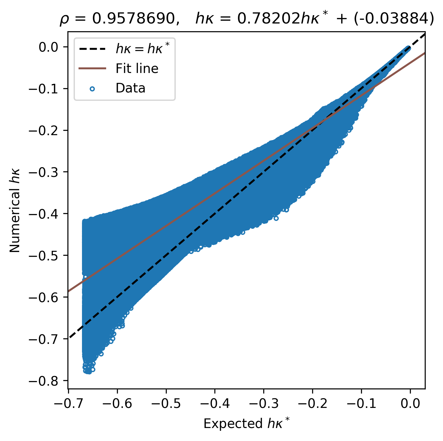
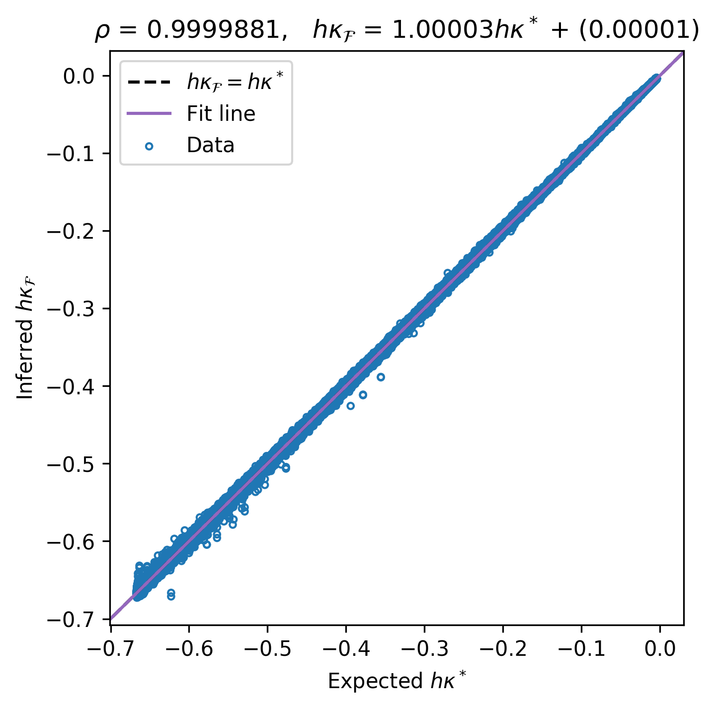
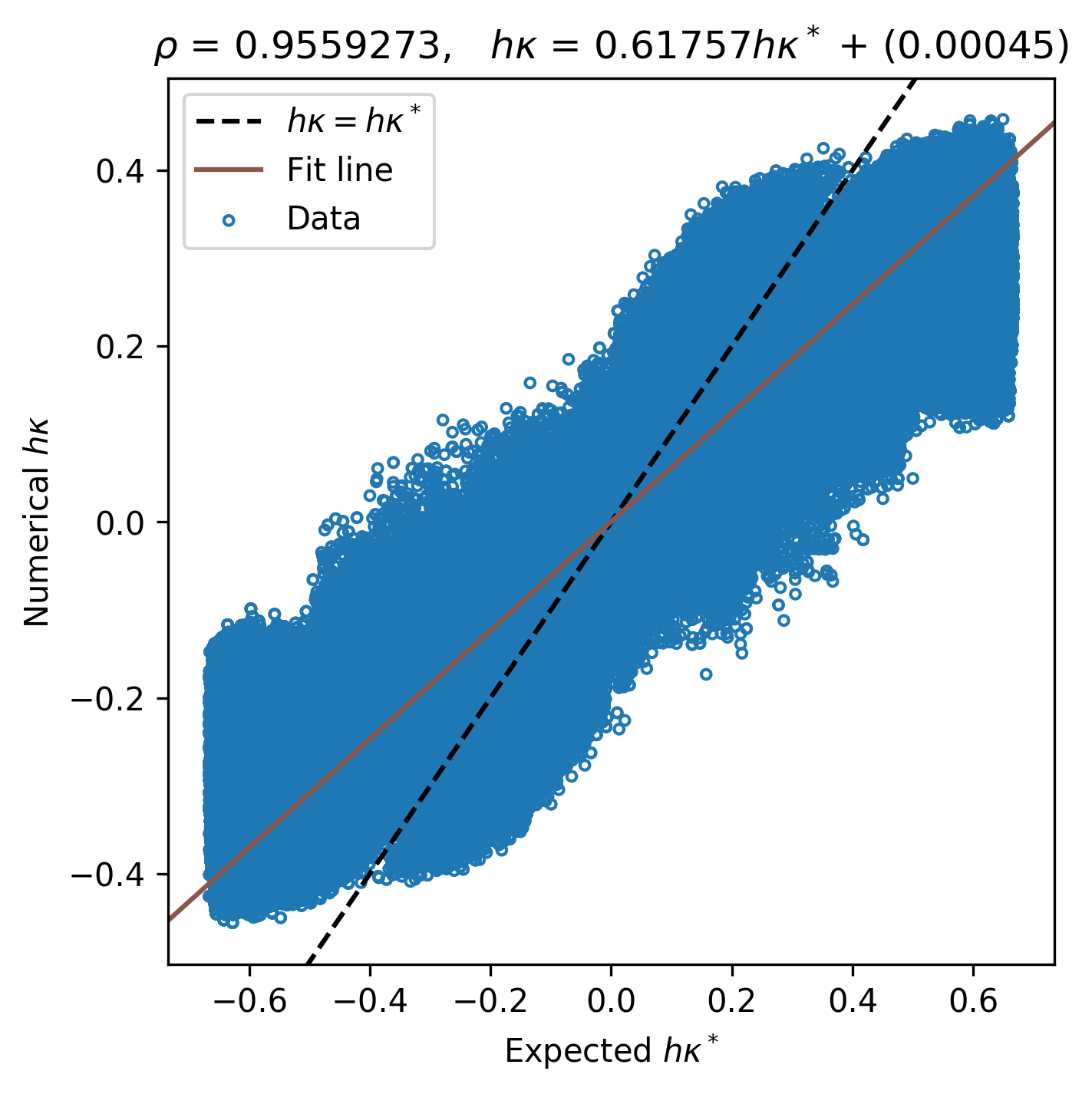
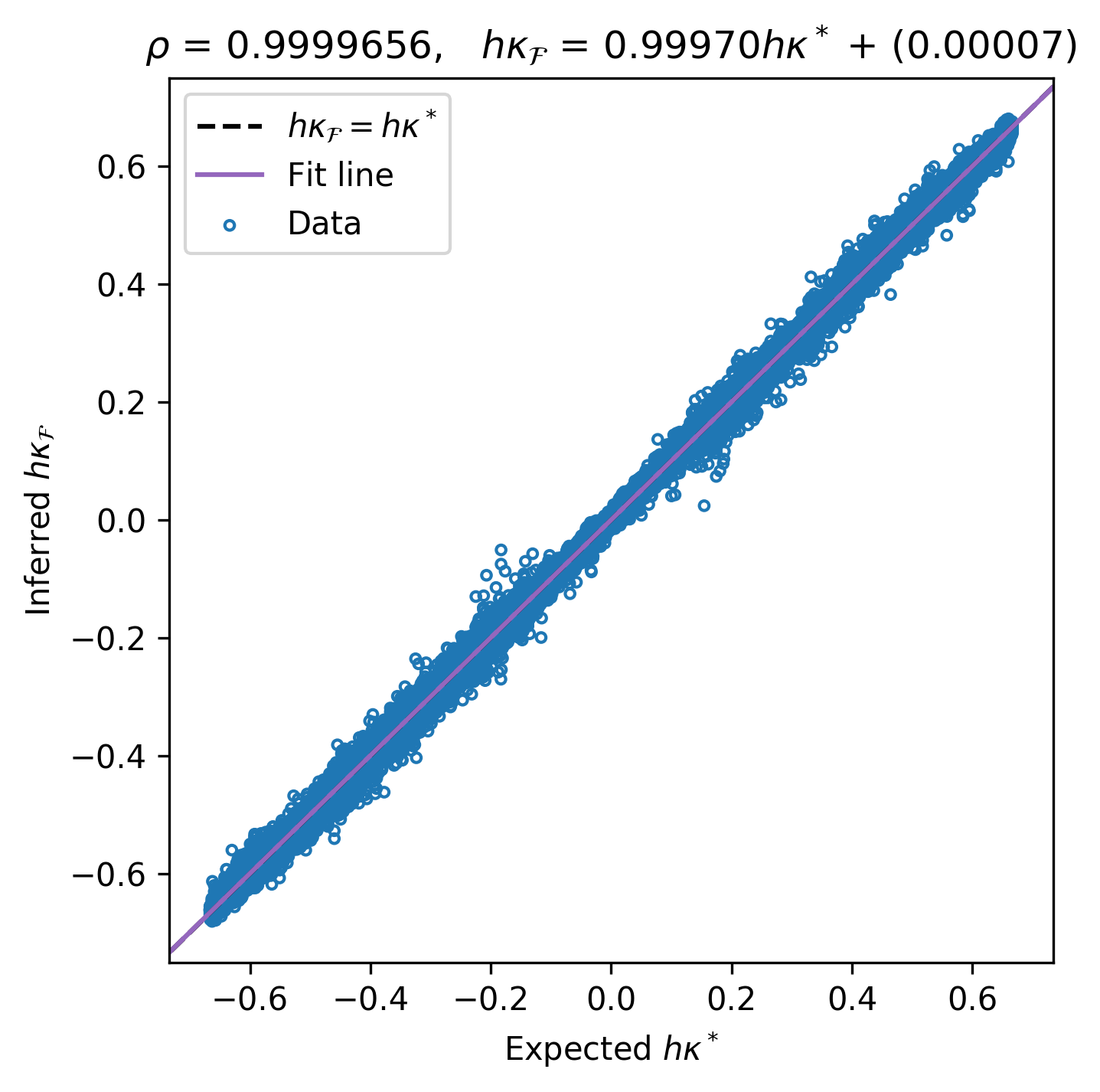
Figure 9 validates the results in table 2 by contrasting the quality of the fit of our neural functions and the numerical baseline. In particular, the higher correlation factors of and demonstrate the ability of our error-quantifiers to fix along under-resolved and steep interface regions. For the interested reader, we have released these and the neural networks trained for other mesh resolutions as HDF5 and Base64-encoded JSON files at https://github.com/UCSB-CASL/Curvature_ECNet_3D. In the same repository, we have provided the preprocessing objects from Algorithm 8 as JSON and pickle files alongside testing data and their supplementary documentation.
5.1 Geometrical tests
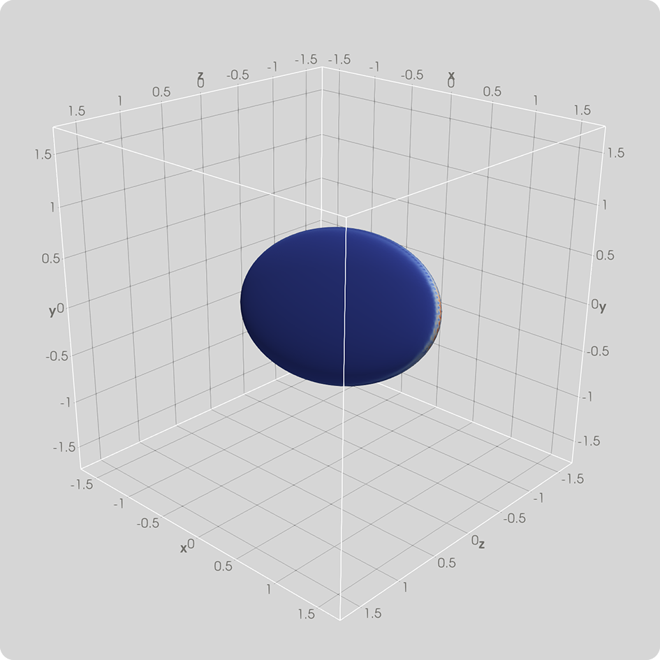
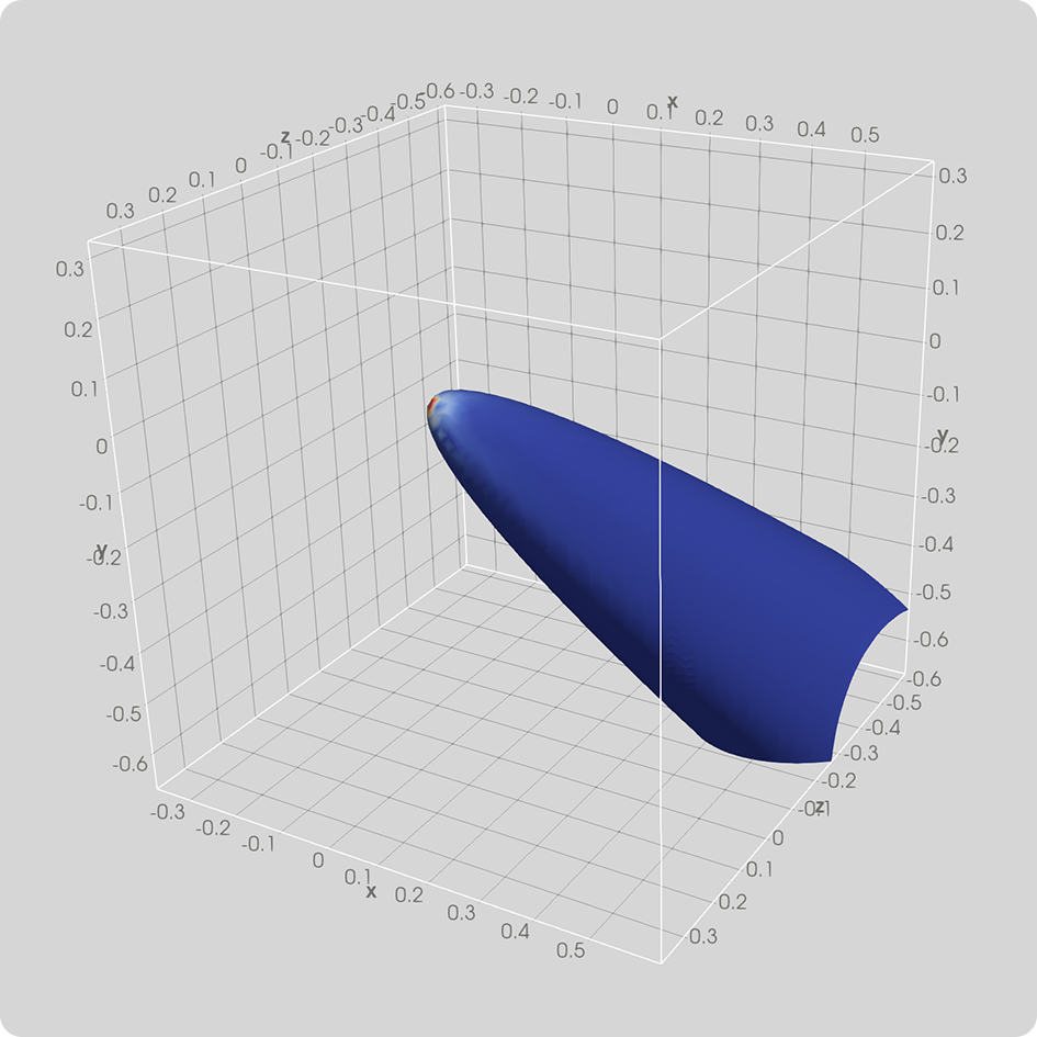
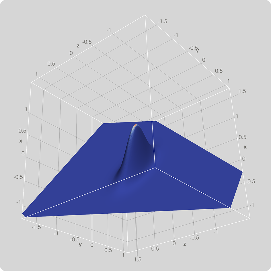
In this section, we evaluate our hybrid strategy with three stationary geometries not accounted for during training. These geometries—an ellipsoid, a paraboloid, and a Gaussian shown in fig. 10—represent the zero-isosurfaces of their respective level-set functions. Then, we validate the MLCurvature() routine on a sphere morphing into an ellipsoid with large mean curvatures at its semi-axes. In principle, our starting point is for all scenarios, but we have introduced and when appropriate to compare the conventional approach and Algorithm 2.
Before addressing each case, we briefly describe the general experimental setup. First, we prescribe a random affine transformation (see eqs. 17 and 18) and discretize with adaptive Cartesian grids accordingly. Such a discretization must enforce a uniform band of half-width around the affine-transformed interface, where . Then, we evaluate by calculating “exact” signed distances to at least within a (linearly approximated) shell of half-width . These normal distances have resulted from solving the nearest-location problem with dlib, as in Algorithms 4 and 6. After that, we perturb the nodal level-set values with uniform random noise in the range of , where . Finally, we redistance our level-set function with steps and estimate at with Algorithm 2 for all the interface nodes. Note that we have continued to use to distinguish non-saddle from saddle stencils.
5.1.1 An ellipsoidal interface
Consider an ellipsoid parametrized in spherical coordinates by
| (25) |
where is the reduced latitude (as measured from the -plane), is the longitude, and , , and are the semi-axis lengths in its canonical frame [98]. Furthermore, suppose is some query point on the surface. Then, we can derive and evaluate the mean and Gaussian curvatures at as
| (27) |
| (28) |
where yields the shortest distance between (expressed in terms of ) and the surface. This definition partitions the computational domain in such a way that lies inside , and corresponds to the exterior space. Moreover, since , we expect mostly non-saddle stencils enabling in Algorithm 2.
In this experiment, we have chosen , , and , so the local extrema at the -, -, and -intercepts are 0.345182, 0.148637, and . Figure 10(a) pictures the ellipsoid as ’s zero-isosurface while emphasizing regions along where is large. The statistics for our hybrid method and the numerical baseline appear in table 3. For reference, we have included the error metrics and costs for estimating mean curvatures numerically at twice and four times the grid resolution (i.e., at ). Furthermore, we have wall-timed131313In C++ 14, we enabled compiling optimization with the options -O2 -O3 -march=native. the evaluations using three MPI tasks on a MacBook Pro with six 2.2 GHz Intel i7 cores and 16 GB RAM. We have selected the best runtimes out of ten trials in all the assessments in this section.
| MAE | MaxAE | Performance | |||||||
| Method | Improv. Factor | Improv. Factor | Time (secs.) | Cost (%) | |||||
| MLCurvature() | 6 | - | - | 6.5107 | - | ||||
| Baseline | 6 | 9.74 | 8.70 | 4.7991 | |||||
| 7 | 2.82 | 3.56 | 19.3433 | ||||||
| 8 | 1.21 | 1.22 | 85.8928 | ||||||
Table 3 provides the and error norms for and to ease the comparisons between the solvers at the same and different mesh sizes. In particular, the improvement factor column indicates the -error ratio from the baseline to our hybrid inference system. Similarly, the cost column shows how much more () or less () time it takes for the MLCurvature() routine to solve the same problem as the numerical approach. At , for example, our strategy can reduce the estimation error by a factor of at least while incurring an additional overhead of . This inference cost might seem discouraging, but we can justify it by analyzing the rows of and . In this regard, not only does increasing the grid resolution improve the numerical accuracy, but it also has a detrimental effect on the baseline performance. Consider , for instance. In that case, table 3 reveals that the conventional schemes alone cannot guarantee the same precision as MLCurvature(), which now requires one-third of the cost. In addition, the statistics in this table suggest that our proposed method can attain a comparable level of precision to the baseline at four times the mesh size but at of the numerical cost. Figure 11 complements these results by contrasting the quality of the evaluated approximations. Clearly, our solver offers an inexpensive way to offset mean-curvature errors, with no need for further mesh refinement.
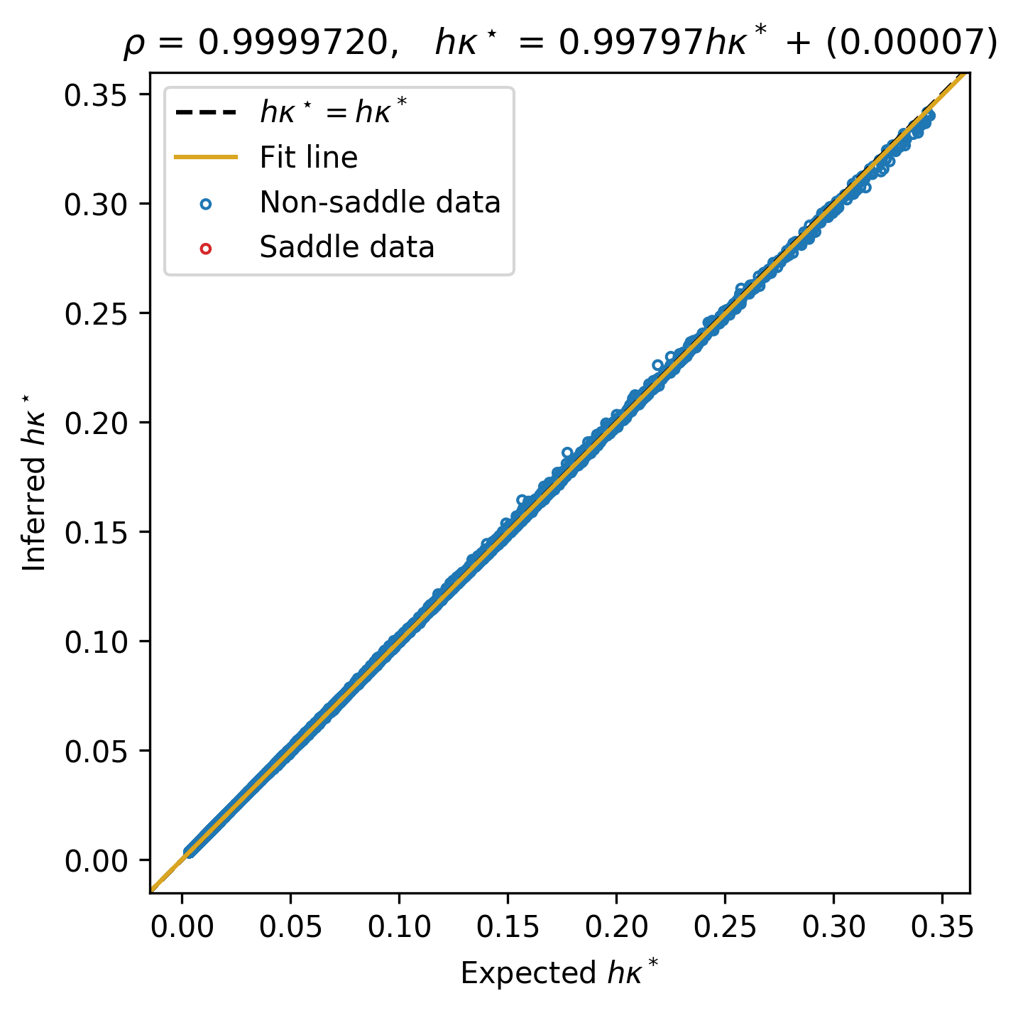
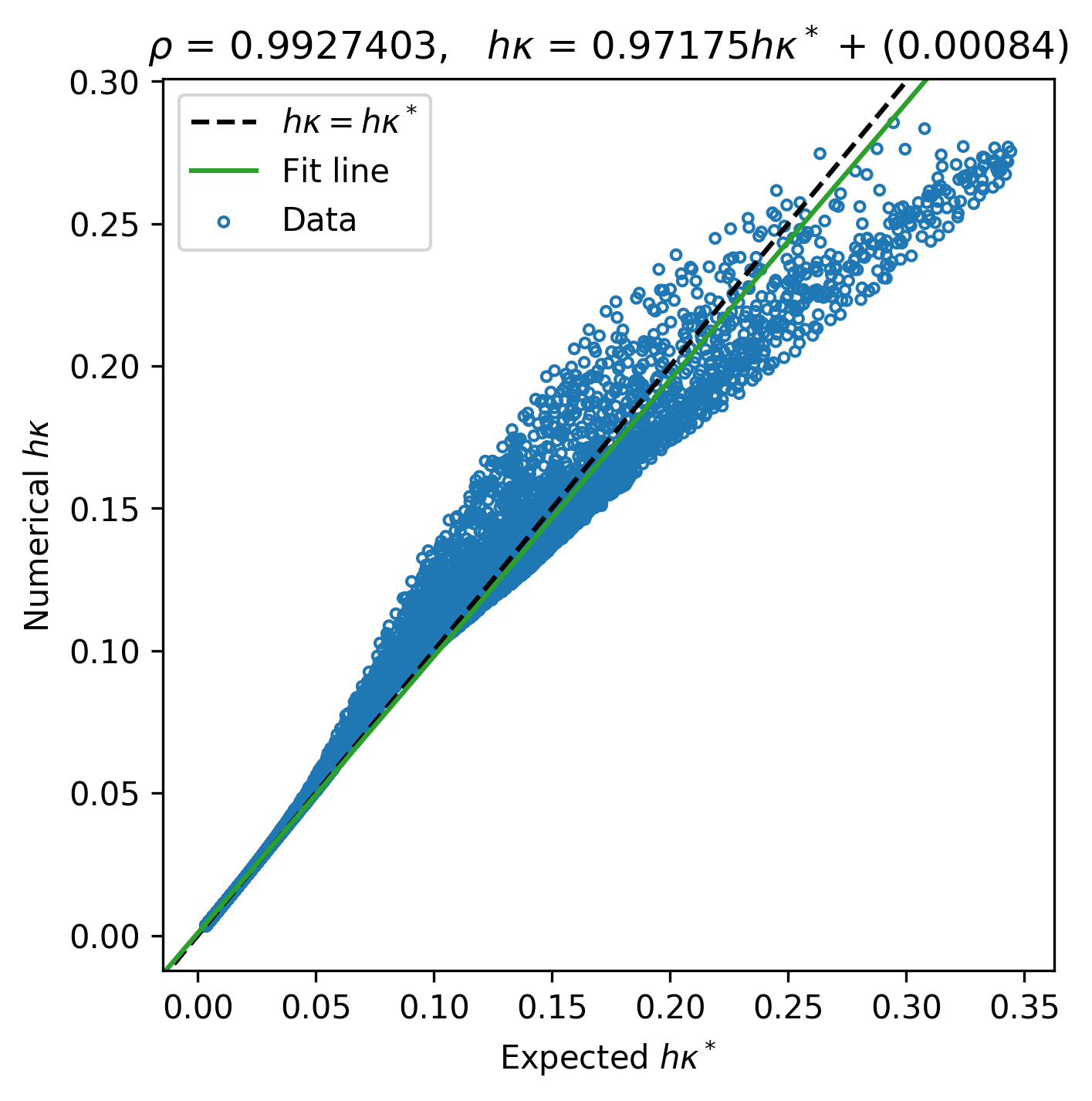
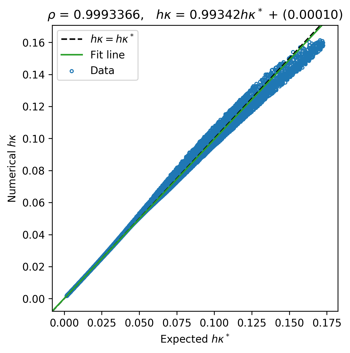
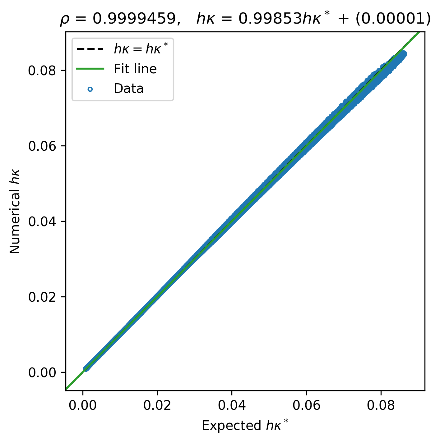
5.1.2 A paraboloidal interface
Next, consider a paraboloid denoted by the Monge patch
| (29) |
where and are positive shape parameters. Expressing the paraboloidal surface with eq. 29 allows us to find the exact mean and Gaussian curvatures at any query point with
| (30) |
where for all , at least theoretically. In practice, the latter implies more frequent activations of the non-saddle path in Algorithm 2.
The patch definition in eq. 29 leads us to the level-set function
| (31) |
where is given in the representation of the local coordinate system . Like in eq. 23, partitions the computational domain into above and right beneath it.
In this test, we have selected and so that at the trough. In addition, we have introduced a customized parameter to set the paraboloid’s height. This parameter has helped us bound and keep the entire affine-transformed surface from to within the computational domain. Figure 10(b) illustrates the paraboloidal interface in the world coordinate system. In analogy to Section 5.1.1, the mean-curvature accuracy results and the performance metrics for this experiment appear in table 4.
| MAE | MaxAE | Performance | |||||||
| Method | Improv. Factor | Improv. Factor | Time (secs.) | Cost (%) | |||||
| MLCurvature() | 6 | - | - | 0.6854 | - | ||||
| Baseline | 6 | 10.86 | 39.07 | 0.5663 | |||||
| 7 | 2.78 | 15.34 | 1.4223 | ||||||
| 8 | 1.04 | 4.10 | 4.2628 | ||||||
Table 4, once more, confirms the ability of our data-driven strategy to reduce mean-curvature errors significantly. For example, when the paraboloid is embedded in a discretized grid with , we can get error-reduction factors of at least one order of magnitude and up to forty in the and norms. Likewise, as discussed in Section 5.1.1, increasing to 7 and 8 improves the baseline mean-curvature approximations, but not at the same level as the MLCurvature() routine when . Indeed, our hybrid solver yields better estimations than the numerical approach at twice the resolution but requires only half of the cost. Table 4 also corroborates that Algorithm 2 can attain a comparable level of precision to the standard level-set approach at four times the base mesh size, but at of the numerical cost. Lastly, fig. 12 offers another perspective on the quality of the neural and numerical curvature computations by plotting them against . As expected, the baseline’s entries look noisier than ours at , particularly when handling steep interface regions.
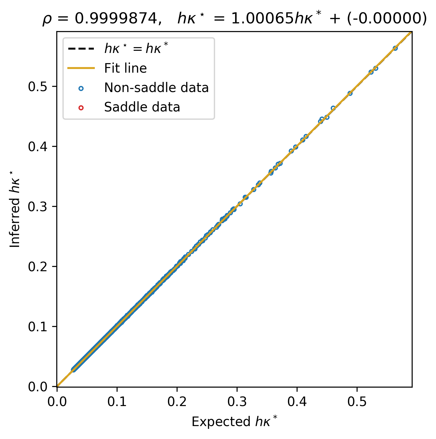
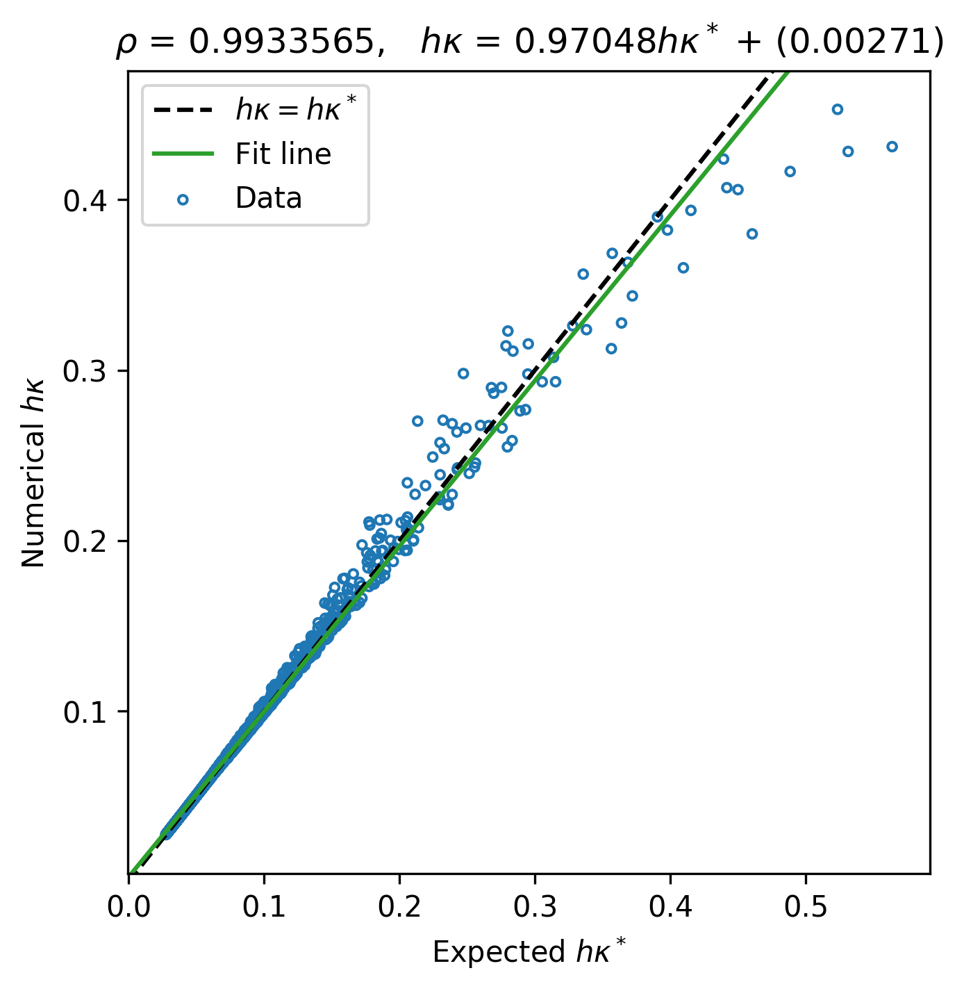
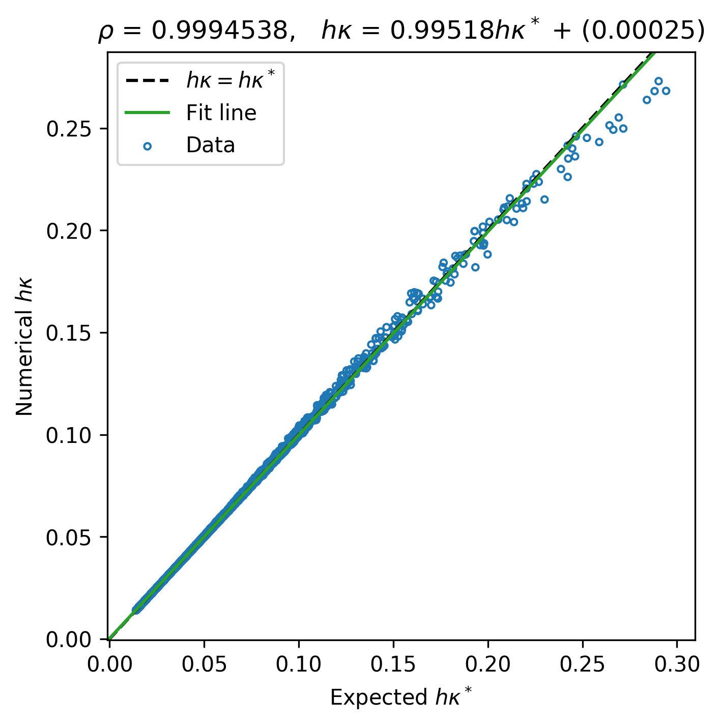
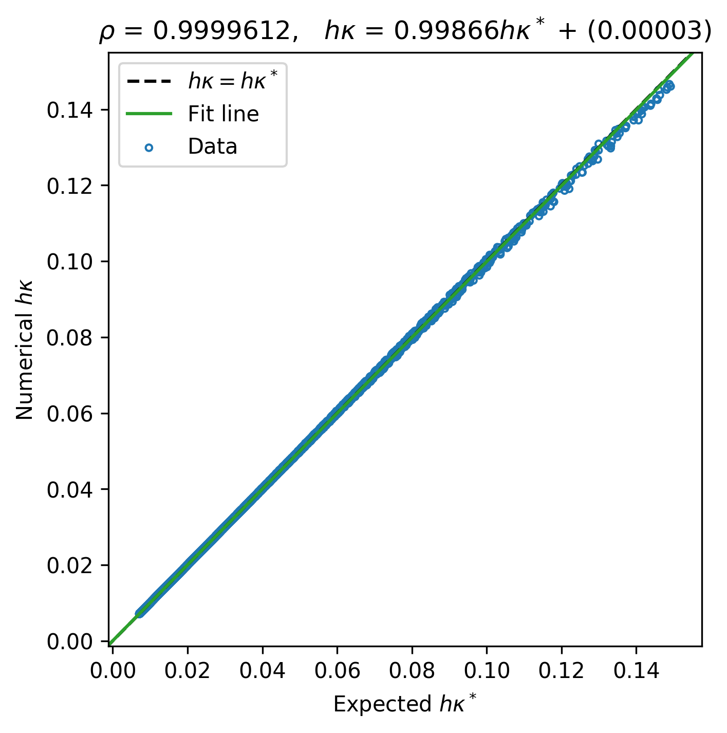
5.1.3 A Gaussian interface
Now, we evaluate the accuracy of the mean-curvature estimations along a Gaussian Monge patch given by
| (32) |
where is the height, and the nonzero and parameters control the spread of the data in the and directions. After applying the procedures from [3] on eq. 32, we arrive at the analytical forms
| (33) |
to calculate the mean and Gaussian curvatures at any . Unlike eqs. 26 and 30, may be positive or negative. This property enables the non-saddle and saddle paths in Algorithm 2 and thus allows us to test our solver’s response when both and partake in the mean-curvature computations.
As before, we can use eq. 32 to construct the level-set function
| (34) |
where is expressed in terms of the local coordinate frame . Equation 34 partitions the computational space into above and right beneath it.
In this experiment, we consider the shape parameters , , and so that the desired at the peak reaches . Also, we have ensured that the randomly affine-transformed Gaussian surface inscribed in an elliptical cylinder of semi-axes and is fully contained within the discretized . Here, and denote the locations where (i.e., they define the four ’s saddle points in the and directions). We have approximated these critical points with the Newton–Raphson subroutine provided by the Boost C++ library [99]. Furthermore, we have only accounted for stencils lying inside the limiting cylinder when sampling and gleaning error statistics to keep flat-region overrepresentation at bay.
| MAE | MaxAE | Performance | |||||||
| Method | Improv. Factor | Improv. Factor | Time (secs.) | Cost (%) | |||||
| MLCurvature() | 6 | - | - | 7.7799 | - | ||||
| Baseline | 6 | 3.83 | 11.85 | 6.4389 | |||||
| 7 | 1.13 | 6.19 | 27.1916 | ||||||
| 8 | 0.46 | 2.06 | 136.3310 | ||||||
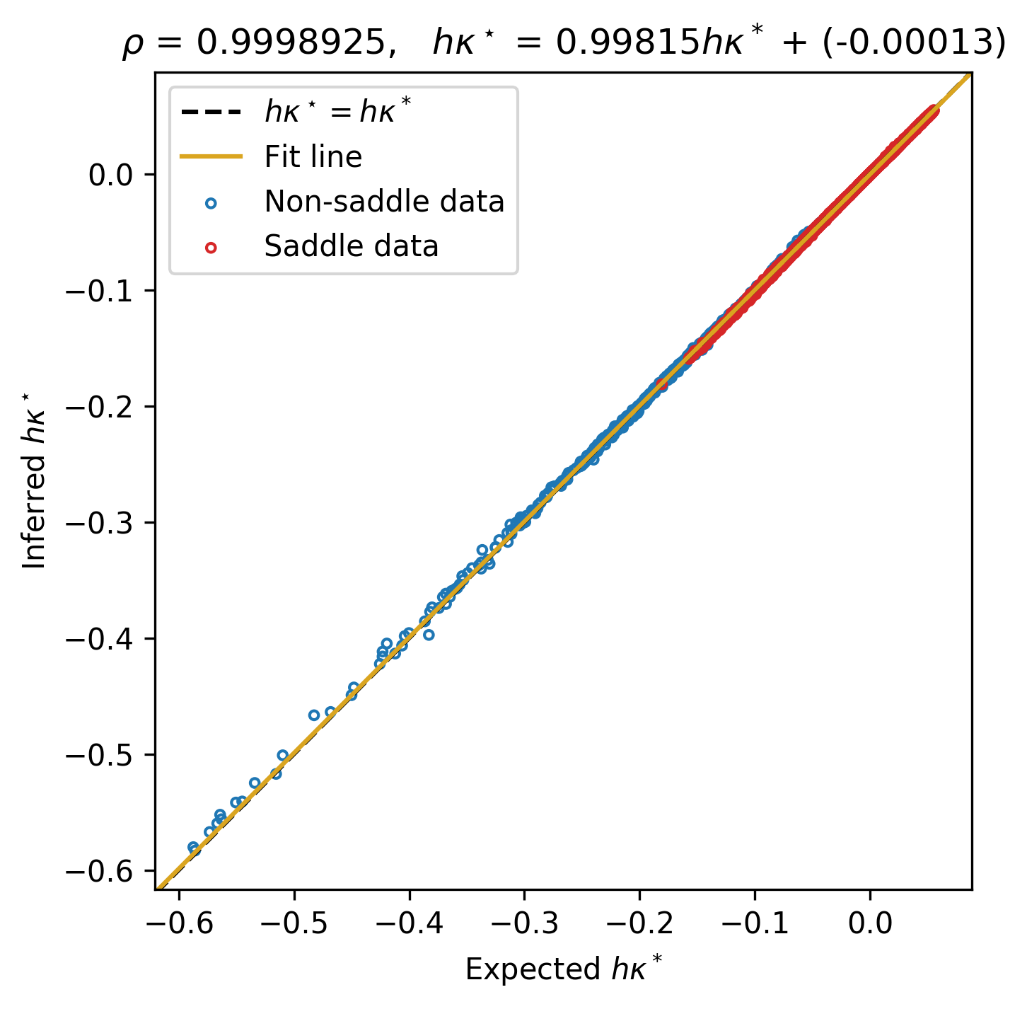
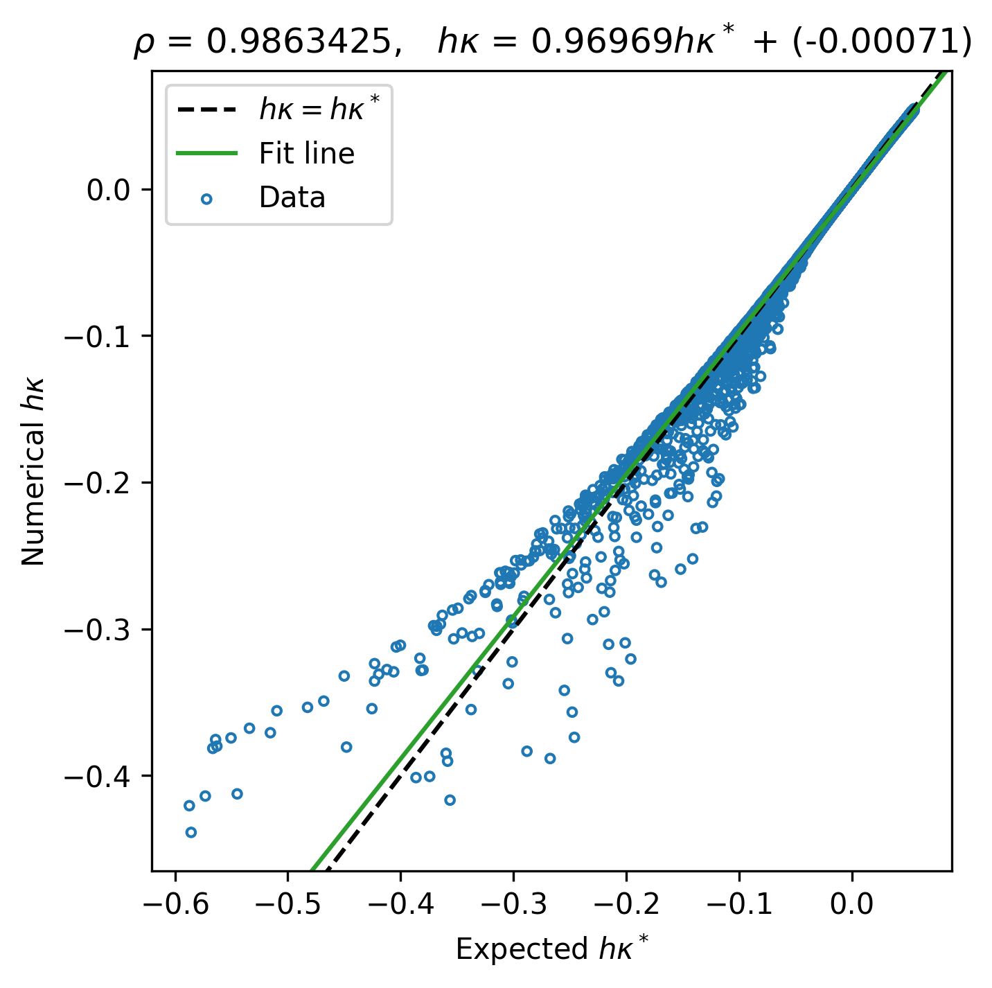
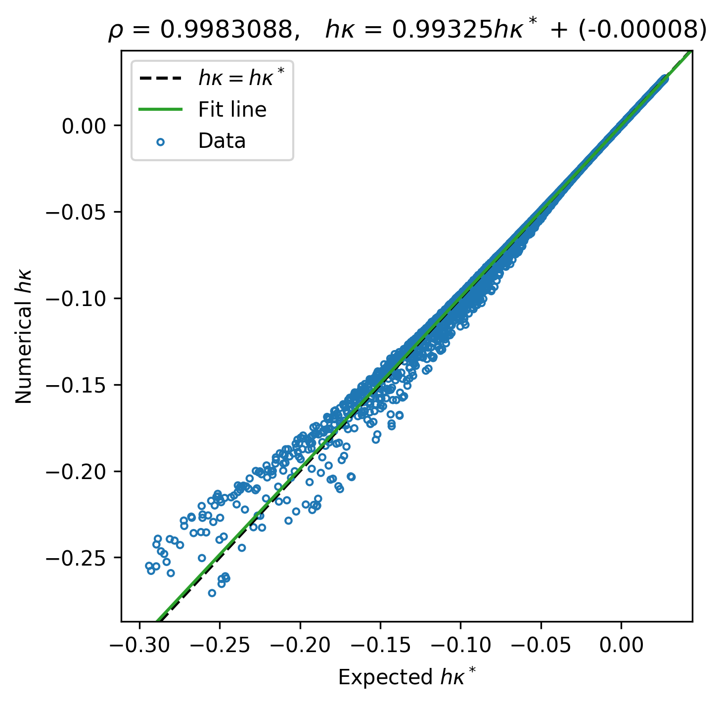
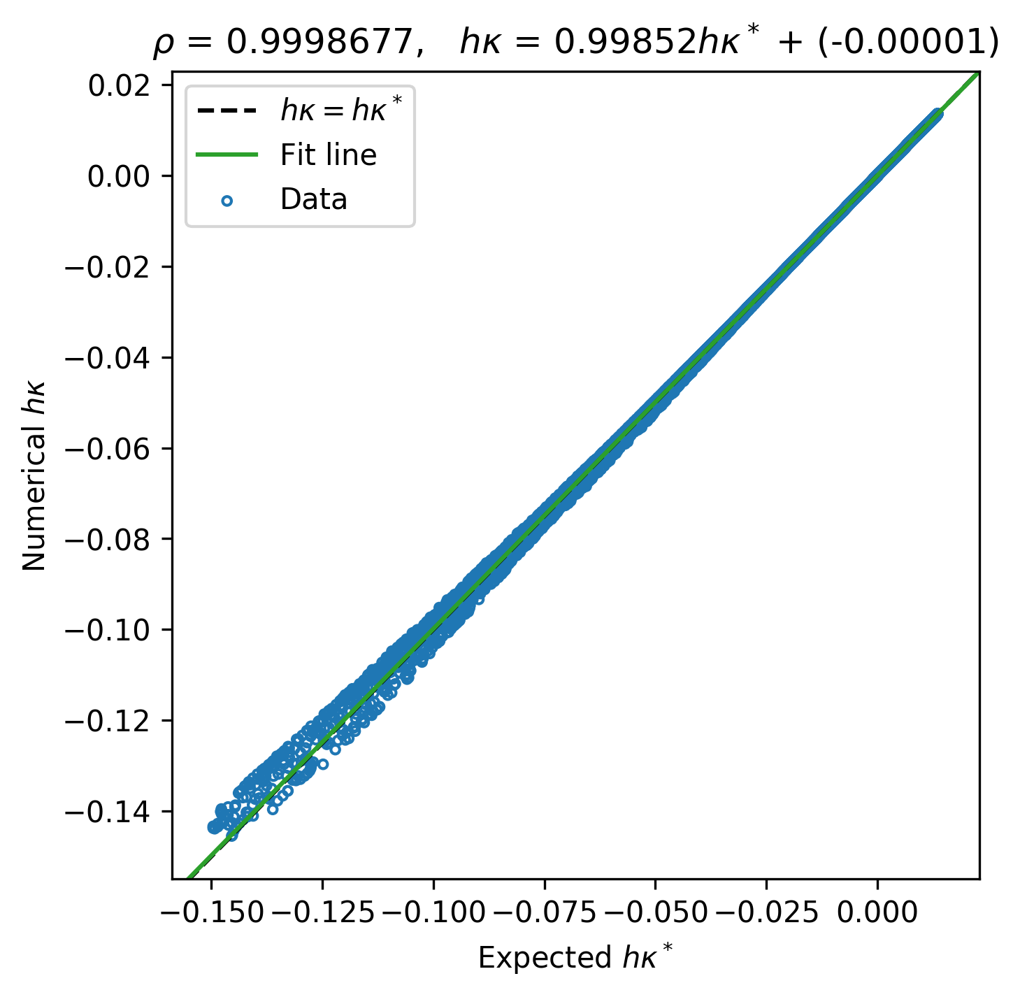
Following the above assumptions, we have summarized the results in table 5 for the Gaussian interface shown in fig. 10(c). These metrics reveal that our approach is again superior to the numerical baseline by at least one order of magnitude in the norm when . Surely, one can narrow this gap by doubling the grid resolution to , but this only quadruples the cost with unsatisfactory results as (see fig. 13(c)). Likewise, reducing the mesh size to enhances the numerical precision significantly, but it raises the computational cost by 17.5 times compared to our Algorithm 2 at . Our strategy is thus more resilient to high-mean-curvature (non-saddle and saddle) regions and can fix such mean-curvature errors without increasing mesh refinement. More importantly, training with saddle surfaces has endowed our solver with the ability to handle a larger variety of instantiated level-set stencils than those considered by other systems tailored only for non-saddle patterns [47]. To conclude, fig. 13 corroborates the statistics in table 5 and facilitates the error analysis and contrast between the baseline and the proposed method. The improvements are remarkable.
5.1.4 A sphere morphing into an ellipsoid
We conclude this series of geometrical experiments with a spherical interface morphing into an ellipsoid. Initially, we consider a level-set function, such as eq. 13, with a randomly shifted spherical zero-isosurface of radius . Then, we steadily interpolate from to , , and so that transforms into in eq. 28 after 51 steps. In each stage, we have perturbed the nodal level-set values with random uniform noise and reinitialized with ten iterations, as noted in the preamble of Section 5.1.
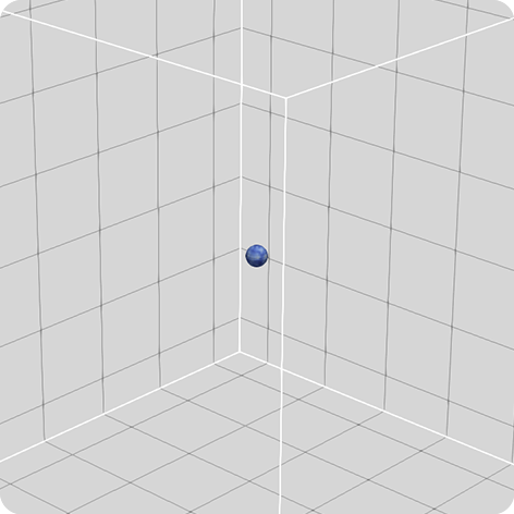
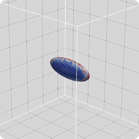
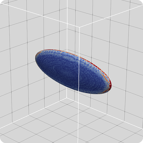
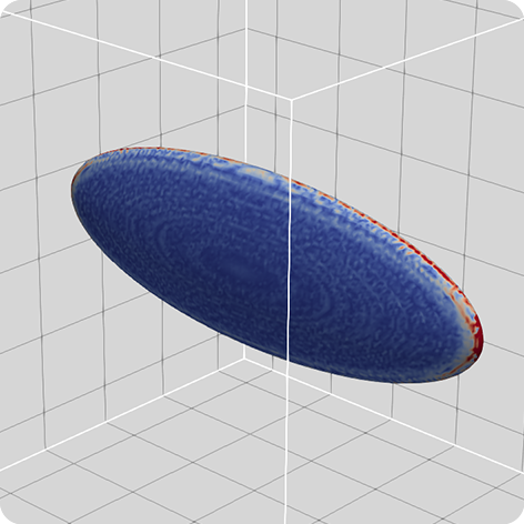
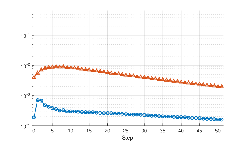
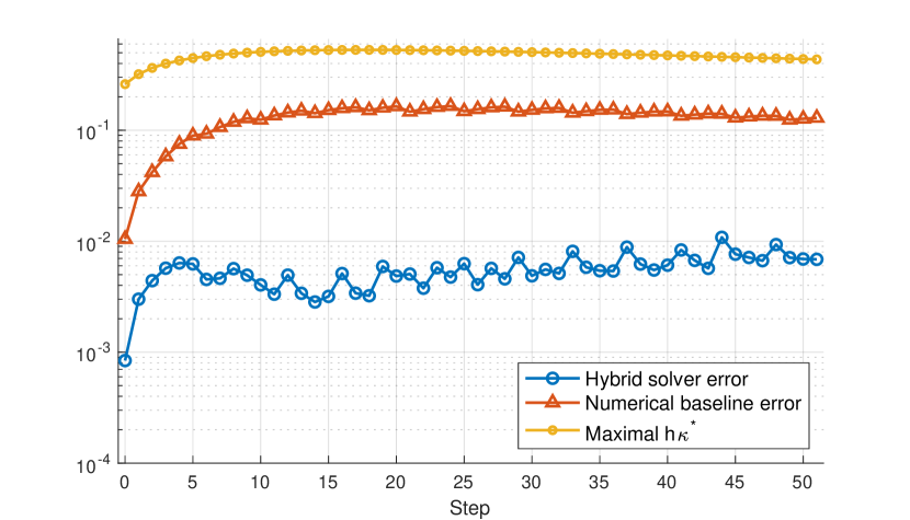
The top row in fig. 14 depicts the evolution of the morphing surface with a few snapshots. In particular, we have emphasized the regions where the baseline schemes exhibit significant mean-curvature errors. Figure 14 also asserts the ability of our neural networks to reduce by contrasting the numerical and hybrid and error norms in a couple of charts. These plots mostly demonstrate a sustained accuracy improvement of about one order of magnitude. However, the hybrid solver’s MaxAE growing trend in fig. 14(f) reveals an underlying problem with and that we have not analyzed yet. In the next section, we address this issue from the perspective of two convergence use cases.
5.2 Convergence tests
Next, we verify the accuracy and analyze the convergence of Algorithm 2 on spherical interfaces. The first test deals with octree-based meshes, where and . After that, we validate our strategy on arbitrary uniform grids where the latter condition no longer holds.
5.2.1 Case 1: Relative errors on compatible adaptive grids
First, we consider the convergence test proposed by Karnakov et al. in Section 3.1 in [13]. Karnakov and coauthors have developed a hybrid mean-curvature solver for the VOF representation using strings of particles in equilibrium and height functions. Their method has been shown to outperform the combination of height functions and parabolic fitting [100] for under-resolved interfaces in multiphase flows.
In this test, we define a spherical-interface level-set function of radius , as in eq. 13. Then, we vary the number of cells per radius, , and evaluate one hundred randomly shifted instances of the same surface. The procedure for generating these instances is analogous to Algorithm 3. Here, we extract their centers (component by component) from a uniform random distribution between and . Afterward, we discretize with an adaptive grid , enforcing a uniform band of half-width around . Next, we find the exact signed distances to , reinitialize with iterations, and compute mean curvatures along the surface. For each , we have constructed with one cubic octree so that , , and . The relative metrics collected for every ratio include
| (35) |
where is the set of all interface nodes.
Incidentally, we have chosen because it is almost the smallest sphere we can resolve for . Furthermore, we have gathered results using the MLPs optimized for and the models trained individually for the other resolutions. To fit these additional estimators, we have followed the methodologies presented in Section 4 by changing where appropriate. The reader may find all these neural networks at https://github.com/UCSB-CASL/Curvature_ECNet_3D.
| MLCurvature() () | Order | MLCurvature() () | Order | Baseline | Order | |
| - | - | - | ||||
| -0.56 | -0.63 | 1.28 | ||||
| -0.20 | 0.17 | 1.60 | ||||
| -0.49 | -0.86 | 1.75 | ||||
| -0.72 | -0.99 | 1.73 |
| MLCurvature() () | Order | MLCurvature() () | Order | Baseline | Order | |
| - | - | - | ||||
| -0.19 | -0.19 | 1.09 | ||||
| 0.34 | 0.77 | 1.66 | ||||
| -0.96 | -1.42 | 1.86 | ||||
| -1.47 | -0.98 | 1.25 |
Tables 6 and 7 summarize the relative errors and the order of convergence of our hybrid inference system and the baseline. To distinguish the neural networks used with Algorithm 2, we have labeled their training resolution with and . The wildcard denotes matching training and testing mesh sizes. Tables 6 and 7 and the accompanying plots in fig. 15 reveal the superiority of our error-correcting strategy over the baseline and Karnakov’s schemes along under-resolved interface sectors. For , for example, the and error norms can decrease at least by a factor of 7.7. In addition, these results demonstrate that neural networks fitted to data from a prescribed can be used with negligible accuracy variations in other discretizations. This observation is important because the methodology outlined in Section 4 can free the scientist from building data sets and training pairs of neural models for each distinct they plan to support. Consequently, our strategy is more cost-effective than constructing resolution-dependent dictionaries of MLPs, as proposed in [48, 2].
Tables 6 and 7 and fig. 15 also corroborate the lack of convergence in the machine learning solution, as noted in prior studies for [2, 1]. In fact, our relative accuracy deteriorates rather quickly as , thus suggesting the need for a better blending strategy between and (see algorithms 2 to 2 Algorithm 2). There are several possibilities in this regard. Karnakov and coauthors, for instance, have used conventional mechanisms to switch between their particle approximation and height functions when computing curvatures in [13]. In contrast, Buhendwa et al. have resorted to neural networks to decide when to reconstruct a level-set interface via machine learning or with consistent numerical procedures [53]. Enforcing consistency in our MLCurvature() routine is a topic that deserves further investigation, possibly incorporating classifiers like those in [101, 102, 53].
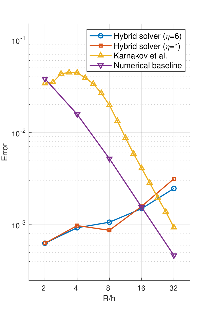
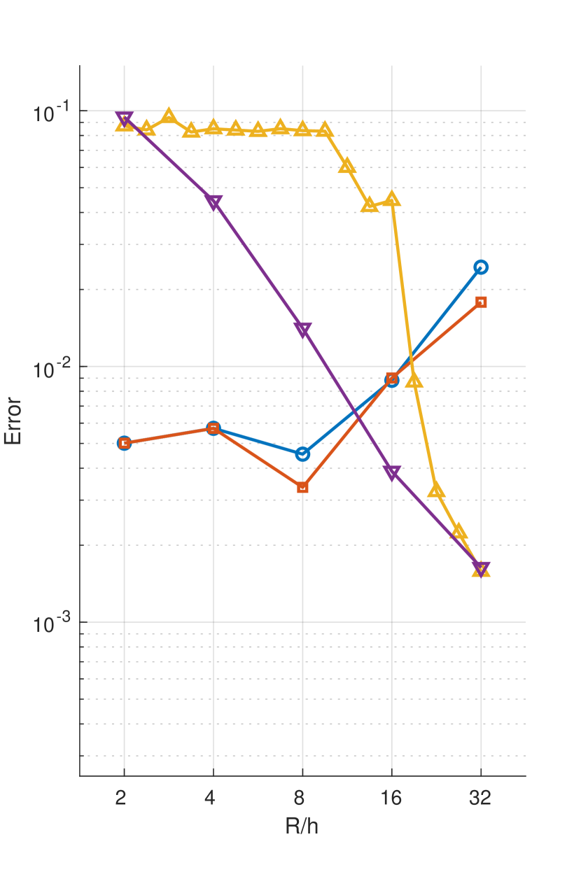
5.2.2 Case 2: Absolute errors on arbitrary uniform grids
To conclude, we demonstrate that Algorithm 2 works on uniform grids where is unconstrained. This last test recreates the assessment in Section 5.3 in [40], which considers the domain and the level-set field defined by
| (36) |
Equation 36 has a spherical interface of radius centered at the origin, but it is not a signed distance function. Consequently, we have reinitialized with iterations, as in [40], and then computed mean curvatures at with four uniform grid resolutions. Tables 8 and 9 summarize the convergence results when using our models for and an initial mesh with cubic cells. Note we have not perturbed the level-set values or the geometry as before. In addition, we provide our statistics in terms of (not ).
| Cell count | MLCurvature() | Order | Baseline | Order |
| - | - | |||
| 0.88 | 0.71 | |||
| 0.06 | 1.74 | |||
| -0.05 | 1.77 |
| Cell count | MLCurvature() | Order | Baseline | Order |
| - | - | |||
| -0.34 | 0.18 | |||
| 0.51 | 1.98 | |||
| -0.81 | 1.63 |
Tables 8 and 9 show that our hybrid inference system works transparently across grid resolutions after training and . They also confirm that our strategy is superior to the baseline when resolving steep mean curvatures. In particular, these metrics indicate that we can improve the numerical estimations for up to one order of magnitude in the and norms for relatively coarse meshes. However, these statistics and fig. 16 reiterate that our solver is not consistent. For a better hybrid method, we should be able to detect well-resolved stencils with reliable mean-curvature estimations. Then, we could fall back to the standard level-set approach and converge to the correct answer as .
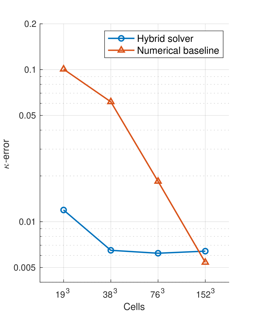
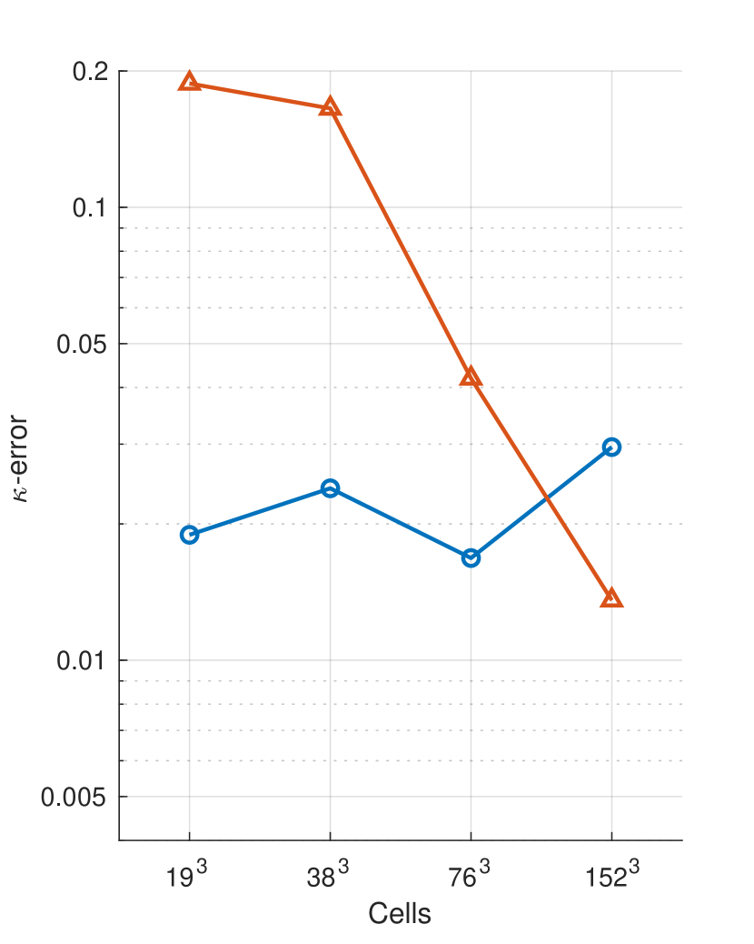
6 Conclusions
We have introduced a machine learning strategy to enhance mean-curvature computations in the level-set representation in . Our approach entails optimizing and deploying error-quantifying neural networks that improve numerical mean-curvature estimations, , at the interface, regardless of the mesh size. Unlike [47] in the VOF framework, these models leverage local level-set and gradient, as well as other geometrical information within a novel hybrid inference system. In line with [53], our solver also enforces symmetry by blending multiple inferred estimations and the standard approximation selectively.
To minimize our solver’s time-space complexity, we have tackled the mean-curvature problem from two perspectives. These depend on whether the Gaussian curvature associated with an interface node is (approximately) nonnegative or negative. The former (non-saddle) case is simpler to handle [2, 1] because its baseline error grows monotonically with . This feature has helped increase neural capacity by training only on the negative mean-curvature spectrum. Likewise, it has allowed us to convex-combine the machine-learning solution and baseline approximations in Algorithm 2 when . Saddle patterns (i.e., ), on the other hand, do not offer the same flexibility. Hence, we have fitted separate estimators, using the full spectrum for our saddle model. Pattern separability has thus led us to design data-generative routines that yield learning tuples from spherical, sinusoidal, and hyperbolic-paraboloidal interfaces. In this regard, Section 4 has introduced the corresponding procedures to build well-balanced data sets with a randomized strategy. Similarly, we have presented other technical aspects to train and realize our two kinds of neural functions and port their preprocessing artifacts into level-set applications.
Experiments with stationary, steep- geometries have confirmed our models’ ability to fix the numerical error in the conventional level-set approach. In particular, we have observed accuracy improvements of around one order of magnitude in the norm along under-resolved interface regions. Also, we have shown that our proposed solver can estimate sharp mean curvatures at an unparalleled level of precision, even if one doubles the mesh resolution to reduce the baseline mean-curvature error. Our relative accuracy, however, can deteriorate as stencils become more well-resolved. On this matter, the convergence tests in the second half of Section 5 have underlined the lack of consistency in Algorithm 2 as . Making the MLCurvature() routine consistent is thus the natural next step in our research. Although various possibilities exist, we have narrowed down this problem to identifying well-resolved patterns so that we can fall back to the standard mean-curvature estimations when appropriate. Such an identification function could be as simple as a quality metric [103, 21, 32, 33] or as sophisticated as a neural binary classifier [101, 102, 53].
To conclude, we comment on a potential enhancement to the data-generating strategy from Sections 4.2.1 to 4.2.3. Although comprehensive, our learning data sets are only well-balanced with respect to . Other latent distributions, like those of and , could be heavily skewed and impair generalization. For this reason, we have entertained the possibility of using two-dimensional histograms to level up sample frequencies along and either or . Then, one would expect more robust neural responses across broader error and mean-curvature spectra.
Acknowledgements
This research was funded by ONR MURI N00014-11-1-0027 and NSF CBET-EPSRC 2054894. This work used the Extreme Science and Engineering Discovery Environment (XSEDE), which is supported by National Science Foundation grant number ACI-1053575, for resources at the Texas Advanced Computing Center (TACC).
References
- [1] L. Á. Larios-Cárdenas and F. Gibou. Error-correcting neural networks for two-dimensional curvature computation in the level-set method. J. Sci. Comput., 93(1):6, October 2022.
- [2] L. Á. Larios-Cárdenas and F. Gibou. A hybrid inference system for improved curvature estimation in the level-set method using machine learning. J. Comput. Phys., 463:111291, August 2022.
- [3] A. Gray, E. Abbena, and S. Salamon. Modern Differential Geometry of Curves and Surfaces with MATHEMATICA. Studies in Advanced Mathematics. Chapman & Hall/CRC, Boca Raton, FL, third edition, 2006.
- [4] S. Osher and J. A. Sethian. Fronts propagating with curvature-dependent speed: Algorithms based on Hamilton–Jacobi formulations. J. Comput. Phys., 79(1):12–49, November 1988.
- [5] S. Popinet. Numerical models of surface tension. Annu. Rev. Fluid Mech., 50(1):49–75, January 2018.
- [6] A. Friedman. Variational Principles of Free-Boundary Problems. Dover Publications, 2010.
- [7] G. Carinci, A. de Masi, C. Giardinà, and E. Presutti. Free Boundary Problems in PDEs and Particle Systems. SpringerBriefs Math. Springer, Cham, 2016.
- [8] M. Sussman, P. Smereka, and S. Osher. A level set approach for computing solutions to incompressible two-phase flow. J. Comput. Phys., 114(1):146–159, September 1994.
- [9] M. Sussman, E. Fatemi, P. Smereka, and S. Osher. An improved level set method for incompressible two-phase flows. Comput. & Fluids, 27(5-6):663–680, June 1998.
- [10] F. Gibou, L. Chen, D. Nguyen, and S. Banerjee. A level set based sharp interface method for the multiphase incompressible Navier–Stokes equations with phase change. J. Comput. Phys., 222(2):536–555, March 2007.
- [11] M. Theillard, F. Gibou, and D. Saintillan. Sharp numerical simulation of incompressible two-phase flows. J. Comput. Phys., 391:91–118, August 2019.
- [12] F. Gibou, D. Hyde, and R. Fedkiw. Sharp interface approaches and deep learning techniques for multiphase flows. J. Comput. Phys., 380:442–463, March 2019.
- [13] P. Karnakov, S. Litvinov, and P. Koumoutsakos. A hybrid particle volume-of-fluid method for curvature estimation in multiphase flows. Int. J. Multiph. Flow, 125:103209, January 2020.
- [14] R. Egan, A. Guittet, F. Temprano-Coleto, T. Isaac, F. J. Peaudecerf, J. R. Landel, P. Luzzatto-Fegiz, C. Burstedde, and F. Gibou. Direct numerical simulation of incompressible flows on parallel octree grids. J. Comput. Phys., 428:110084, March 2021.
- [15] H. Chen, C. Min, and F. Gibou. A numerical scheme for the Stefan problem on adaptive Cartesian grids with supralinear convergence rate. J. Comput. Phys., 228(16):5803–5818, September 2009.
- [16] J. Papac, F. Gibou, and C. Ratsch. Efficient symmetric discretization for the Poisson, heat and Stefan-type problems with Robin boundary conditions. J. Comput. Phys., 229(3):875–889, February 2010.
- [17] J. Papac, A. Helgadottir, C. Ratsch, and F. Gibou. A level set approach for diffusion and Stefan-type problems with Robin boundary conditions on quadtree/octree adaptive Cartesian grids. J. Comput. Phys., 233:241, January 2013.
- [18] M. Mirzadeh and F. Gibou. A conservative discretization of the Poisson–Nernst–Planck equations on adaptive Cartesian grids. J. Comput. Phys., 274:633–653, October 2014.
- [19] M. Theillard, F. Gibou, and T. Pollock. A sharp computational method for the simulation of the solidification of binary alloys. J. Sci. Comput., 63:330–354, August 2015.
- [20] V. Mallet, D. E. Keyes, and F. E. Fendell. Modeling wildland fire propagation with level set methods. Comput. Math. Appl., 57(7):1089–1101, April 2009.
- [21] P. Macklin and J. Lowengrub. An improved geometry-aware curvature discretization for level set methods: Application to tumor growth. J. Comput. Phys., 215(2):392–401, July 2006.
- [22] F. Boudon, J. Chopard, O. Ali, B. Gilles, O. Hamant, A. Boudaoud, J. Traas, and C. Godin. A computational framework for 3D mechanical modeling of plant morphogenesis with cellular resolution. PLoS Comput. Biol., 11(1):e1003950, January 2015.
- [23] S. A. Ocko, A. Heyde, and L. Mahadevan. Morphogenesis of termite mounds. Proc. Natl. Acad. Sci. USA, 116(9):3379–3384, February 2019.
- [24] M. A. Alias and P. R. Buenzli. A level-set method for the evolution of cells and tissue during curvature-controlled growth. Int. J. Numer. Methods Biomed. Eng., 36(1):e3279, January 2020.
- [25] T. F. Chan and L. A. Vese. Active contours without edges. IEEE Trans. on Image Process., 10(2):266–277, February 2001.
- [26] S. Osher and N. Paragios. Geometric Level Set Methods in Imaging, Vision, and Graphics. Springer New York, 1 edition, 2003.
- [27] F. Losasso, F. Gibou, and R. Fedkiw. Simulating water and smoke with an octree data structure. ACM Trans. Graph. (SIGGRAPH Proc.), 23(3):457–462, August 2004.
- [28] F. Gibou, D. Levy, C. Cardenas, P. Liu, and A. Boyer. Partial differential equation-based segmentation for radiotherapy treatment planning. Math. Biosci. Eng., 2(2):209–226, April 2005.
- [29] F. Losasso, T. Shinar, A. Selle, and R. Fedkiw. Multiple interacting liquids. SIGGRAPH ACM TOG, 25(3):812–819, July 2006.
- [30] T. H. N. Le, K. G. Quach, K. Luu, C. N. Duong, and M. Savvides. Reformulating level sets as deep recurrent neural network approach to semantic segmentation. IEEE Trans. on Image Process., 27(5):2393–2407, May 2018.
- [31] Q. Zhang. Construction of robot computer image segmentation model based on partial differential equations. J. of Sensors, 2022:6216423, July 2022.
- [32] K. Y. Lervåg. Calculation of interface curvature with the level-set method. https://arxiv.org/abs/1407.7340, July 2014.
- [33] Å. Ervik, K. Y. Lervåg, and S. T. Munkejord. A robust method for calculating interface curvature and normal vectors using an extracted local level set. J. Comput. Phys., 257, Part A:259–277, January 2014.
- [34] S. Osher and R. Fedkiw. Level Set Methods and Dynamic Implicit Surfaces. Appl. Math. Sci. 153. Springer, Cham, 2002.
- [35] F. Gibou, R. Fedkiw, and S. Osher. A review of level-set methods and some recent applications. J. Comput. Phys., 353:82–109, January 2018.
- [36] R. S. Qin and H. K. Bhadeshia. Phase field method. Materials Sci. Tech., 26(7):803–811, 2010.
- [37] C. W. Hirt and B. D. Nichols. Volume of fluid (VOF) method for the dynamics of free boundaries. J. Comput. Phys., 39(1):201–225, January 1981.
- [38] G. Tryggvason, B. Bunner, A. Esmaeeli, D. Juric, N. Al-Rawahi, W. Tauber, J. Han, S. Nas, and Y.-J. Jan. A front-tracking method for the computations of multiphase flow. J. Comput. Phys., 169(2):708–759, May 2001.
- [39] W. Bo, X. Liu, J. Glimm, and X. Li. A robust front tracking method: Verification and application to simulation of the primary breakup of a liquid jet. SIAM J. Sci. Comput., 33(4):1505–1524, July 2011.
- [40] A. du Chéné, C. Min, and F. Gibou. Second-order accurate computation of curvatures in a level set framework using novel high-order reinitialization schemes. J. Sci. Comput., 35:114–131, June 2008.
- [41] G. Russo and P. Smereka. A remark on computing distance functions. J. Comput. Phys., 163(1):51–67, September 2000.
- [42] J. Strain. Tree methods for moving interfaces. J. Comput. Phys., 151(2):616–648, May 1999.
- [43] M. Mirzadeh, A. Guittet, C. Burstedde, and F. Gibou. Parallel level-set methods on adaptive tree-based grids. J. Comput. Phys., 322:345–364, October 2016.
- [44] J. Pathak, M. Mustafa, K. Kashinath, E. Motheau, T. Kurth, and M. Day. Using machine learning to augment coarse-grid computational fluid dynamics simulations. https://arxiv.org/abs/2010.00072, October 2020.
- [45] D. Salac and W. Lu. A local semi-implicit level-set method for interface motion. J. Sci. Comput., 35:330–349, June 2008.
- [46] Y. Qi, J. Lu, R. Scardovelli, S. Zaleski, and G. Tryggvason. Computing curvature for volume of fluid methods using machine learning. J. Comput. Phys., 377:155–161, January 2019.
- [47] H. V. Patel, A. Panda, J. A. M. Kuipers, and E. A. J. F. Peters. Computing interface curvature from volume fractions: A machine learning approach. Comput. & Fluids, 193:104263, October 2019.
- [48] L. Á. Larios-Cárdenas and F. Gibou. A deep learning approach for the computation of curvature in the level-set method. SIAM J. Sci. Comput., 43(3):A1754–A1779, May 2021.
- [49] L. Á. Larios-Cárdenas and F. Gibou. Error-correcting neural networks for semi-Lagrangian advection in the level-set method. J. Comput. Phys., 471:111623, December 2022.
- [50] H. L. França and C. M. Oishi. A machine learning strategy for computing interface curvature in front-tracking methods. J. Comput. Phys., 450:110860, February 2022.
- [51] D. L. Youngs. Time-dependent multi-material flow with large fluid distortion. Num. Method Fluid Dyn., 24:273–285, January 1982.
- [52] M. Ataei, M. Bussmann, V. Shaayegan, F. Costa, S. Han, and C. B. Park. NPLIC: A machine learning approach to piecewise linear interface construction. Comput. & Fluids, 223:104950, June 2021.
- [53] A. B. Buhendwa, D. A. Bezgin, and N. A. Adams. Consistent and symmetry preserving data-driven interface reconstruction for the level-set method. J. Comput. Phys., 457:111049, May 2022.
- [54] C. C. Aggarwal. Neural Networks and Deep Learning – A Textbook. Springer, Cham, 2018.
- [55] G.-S. Jiang and D. Peng. Weighted ENO schemes for Hamilton–Jacobi equations. SIAM J. Sci. Comput., 21(6):2126–2143, 2000.
- [56] R. Courant, E. Isaacson, and M. Rees. On the solution of nonlinear hyperbolic differential equations by finite differences. Comm. Pure Appl. Math., 5:243–255, August 1952.
- [57] A. Wiin-Nielsen. On the application of trajectory methods in numerical forecasting. Tellus, 11(2):180–196, 1959.
- [58] E. Albin, R. Knikker, S. Xin, C. O. Paschereit, and Y. D’Angelo. Computational assessment of curvatures and principal directions of implicit surfaces from 3D scalar data. In M. Floater, T. Lyche, M.-L. Mazure, K. Mørken, and L. L. Schumaker, editors, Mathematical Methods for Curves and Surfaces, volume 10521 of Lecture Notes in Comput. Sci., pages 1–22, Cham, October 2017. Springer International Publishing.
- [59] R. Goldman. Curvature formulas for implicit curves and surfaces. Comput. Aided Geom. Des., 22(7):632–658, October 2005.
- [60] C. Min and F. Gibou. A second order accurate level set method on non-graded adaptive Cartesian grids. J. Comput. Phys., 225(1):300–321, July 2007.
- [61] C.-W. Shu and S. Osher. Efficient implementation of essentially non-oscillatory shock capturing schemes. J. Comput. Phys., 77(2):439–471, August 1988.
- [62] C.-W. Shu and S. Osher. Efficient implementation of essentially non-oscillatory shock capturing schemes, II. J. Comput. Phys., 83(1):32–78, July 1989.
- [63] C. Burstedde, L. C. Wilcox, and O. Ghattas. p4est: Scalable algorithms for parallel adaptive mesh refinement on forests of octrees. SIAM J. Sci. Comput., 33(3):1103–1133, May 2011.
- [64] J. A. Sethian. Level Set Methods and Fast Marching Methods. Cambridge Monogr. Appl. Comput. Math. Cambridge University Press, Cambridge, UK, 2nd edition, 1999.
- [65] M. de Berg, M. van Kreveld, M. Overmars, and O. Schwarzkopf. Computational Geometry - Algorithms and Applications. Springer, Cham, 2nd edition, 2000.
- [66] T. Isaac, C. Burstedde, L. C. Wilcox, and O. Ghattas. Recursive algorithms for distributed forests of octrees. SIAM J. Sci. Comput., 37(5):C497–C531, September 2015.
- [67] C. Min. Local level set method in high dimension and codimension. J. Comput. Phys., 200(1):368–382, October 2004.
- [68] S. Aluru and F. E. Sevilgen. Parallel domain decomposition and load balancing using space-filling curves. In Proceedings Fourth International Conference on High-Performance Computing, HIPC ’97, pages 230–235, Washington, DC, December 1997. IEEE Computer Society.
- [69] W. Gropp, E. Lusk, and A. Skjellum. Using MPI: Portable Parallel Programming with the Message-Passing Interface. MIT Press, Cambridge, MA, 3rd edition, 2014.
- [70] F. Pedregosa, G. Varoquaux, A. Gramfort, V. Michel, B. Thirion, O. Grisel, M. Blondel, P. Prettenhofer, R. Weiss, V. Dubourg, J. Vanderplas, A. Passos, D. Cournapeau, M. Brucher, M. Perrot, and E. Duchesnay. Scikit-learn: Machine learning in Python. J. Mach. Learn. Res., 12:2825–2830, 2011.
- [71] M. Turk and A. Pentland. Eigenfaces for recognition. J. Cogn. Neurosci., 3(1):71–86, January 1991.
- [72] D. S. Parker. Exploring the Matrix – Adventures in Modeling with Matlab. UCLA Course Reader Solutions, January 2016.
- [73] A. Önder and P. L.-F. Liu. Deep learning of interfacial curvature: A symmetry-preserving approach for the volume of fluid method. https://arxiv.org/abs/2206.06041, June 2022.
- [74] S. Balay, S. Abhyankar, M. F. Adams, J. Brown, P. Brune, K. Buschelman, L. Dalcin, A. Dener, V. Eijkhout, W. D. Gropp, D. Karpeyev, D. Kaushik, M. G. Knepley, D. A. May, L. Curfman McInnes, R. Tran Mills, T. Munson, K. Rupp, P. Sanan, B. F. Smith, S. Zampini, H. Zhang, and H. Zhang. PETSc. https://www.mcs.anl.gov/petsc, September 2019. v3.12.0.
- [75] Jr. F. S. Hill. Computer Graphics Using OpenGL. Prentice-Hall Inc., 2nd edition, 2001.
- [76] T. Liu, A. W. Moore, A. Gray, and K. Yang. An investigation of practical approximate nearest neighbor algorithms. In Proc. 17th International Conf. NIPS, NIPS’ 04, pages 825–832, Cambridge, MA, USA, December 2004. MIT Press.
- [77] S. M. Omohundro. Five balltree construction algorithms. Technical report, International Computer Science Institute, Berkeley, CA, USA, November 1989.
- [78] D. E. King. Dlib-ml: A machine learning toolkit. J. Mach. Learn. Res., 10:1755–1758, 2009. https://github.com/davisking/dlib. November 2021. v19.22.
- [79] R. Parent. Computer Animation: Algorithms and Techniques. Morgan Kaufmann, 2nd edition, 2008.
- [80] B. Chapman, G. Jost, and R. van der Pas. Using OpenMP: Portable Shared Memory Parallel Programming. Scientific and engineering computation. MIT Press, Cambridge, MA, 2008.
- [81] University of Texas. Texas Advanced Computing Center. https://www.tacc.utexas.edu, August 2022.
- [82] M. Abadi, A. Agarwal, P. Barham, E. Brevdo, Z. Chen, C. Citro, G. S. Corrado, A. Davis, J. Dean, M. Devin, S. Ghemawat, I. Goodfellow, A. Harp, G. Irving, M. Isard, R. Jozefowicz, Y. Jia, L. Kaiser, M. Kudlur, J. Levenberg, D. Mané, M. Schuster, R. Monga, S. Moore, D. Murray, C. Olah, J. Shlens, B. Steiner, I. Sutskever, K. Talwar, P. Tucker, V. Vanhoucke, V. Vasudevan, F. Viégas, O. Vinyals, P. Warden, M. Wattenberg, M. Wicke, Y. Yu, and X. Zheng. TensorFlow: Large-scale machine learning on heterogeneous systems. https://www.tensorflow.org, 2015.
- [83] F. Chollet et al. Keras. https://keras.io, 2015.
- [84] P. Mehta, M. Bukov, C.-H. Wang, A. G. R. Day, C. Richardson, C. K. Fisher, and D. J. Schwab. A high-bias, low-variance introduction to machine learning for physicists. Phys. Rep., 810:1–124, May 2019.
- [85] A. Géron. Hands-on Machine Learning with Scikit-Learn, Keras & TensorFlow: Concepts, Tools, and Techniques to Build Intelligent Systems. O’Reilly, 2nd edition, November 2019.
- [86] W. McKinney. Data structures for statistical computing in Python. In S. van der Walt and J. Millman, editor, Proceedings of the 9th Python in Science Conference, pages 56–61, June 2010. https://pandas.pydata.org.
- [87] Y. A. LeCun, L. Bottou, G. B. Orr, and K.-R. Müller. Efficient BackProp, volume 7700 of Lecture Notes in Comput. Sci., pages 9–48. Springer Berlin Heidelberg, Berlin, Heidelberg, 2012.
- [88] C. Moler. Numerical Computing with MATLAB. The MathWorks, electronic edition, 2013. https://www.mathworks.com/moler/index_ncm.html.
- [89] TensorFlow. TensorFlow v2.0.0 API for Python. https://www.tensorflow.org/versions/r2.0/api_docs/python/tf, October 2020. Last checked in July 2022.
- [90] I. Goodfellow, Y. Bengio, and A. Courville. Deep Learning. MIT Press, 2016. https://www.deeplearningbook.org.
- [91] X. Glorot, A. Bordes, and Y. Bengio. Deep sparse rectifier neural networks. In G. Gordon, D. Dunson, and M. Dudík, editors, Proceedings of the Fourteenth International Conference on Artificial Intelligence and Statistics, volume 15 of Proceedings of Machine Learning Research, pages 315–323, Fort Lauderdale, FL, USA, April 2011. PMLR.
- [92] D. P. Kingma and J. L. Ba. Adam: A method for stochastic optimization. ICLR, pages 1–13, May 2015.
- [93] X. Glorot and Y. Bengio. Understanding the difficulty of training deep feedforward neural networks. In Y. W. Teh and M. Titterington, editors, Proceedings of the Thirteen International Conference on Artificial Intelligence and Statistics, volume 9 of Proceedings of Machine Learning Research, pages 249–256, Chia Laguna Resort, Sardinia, Italy, May 2010. PMLR.
- [94] N. Lohmann. JSON for modern C++. https://github.com/nlohmann/json, August 2020. v3.9.1.
- [95] T. Hermann. Frugally-deep. https://github.com/Dobiasd/frugally-deep, February 2021. v0.15.2.
- [96] Z. Xianyi and M. Kroeker. OpenBLAS: An optimized BLAS library. https://github.com/xianyi/OpenBLAS, July 2021. v0.3.17.
- [97] Intel Corporation. Developer reference for Intel® oneAPI Math Kernel Library - C: cblas_?gemm. https://www.intel.com/content/www/us/en/develop/documentation/onemkl-developer-reference-c/top/blas-and-sparse-blas-routines/blas-routines/blas-level-3-routines/cblas-gemm.html, May 2022. Last checked in July 2022.
- [98] R. Nürnberg. Distance from a point to an ellipsoid. https://www.ma.ic.ac.uk/~rn/distance2ellipse.pdf, 2006. Last checked in July 2022.
- [99] The Boost Community. Boost C++ libraries. https://www.boost.org, August 2019. v1.71.0.
- [100] S. Popinet. An accurate adaptive solver for surface-tension-driven interfacial flows. J. Comput. Phys., 228(16):5838–5866, September 2009.
- [101] D. Ray and J. S. Hesthaven. An artificial neural network as a troubled-cell indicator. J. Comput. Phys., 367:166–191, August 2018.
- [102] N. R. Morgan, S. Tokareva, X. Liu, and A. Morgan. A machine learning approach for detecting shocks with high-order hydrodynamic methods. AIAA SciTech Forum, January 2020.
- [103] P. Macklin and J. Lowengrub. Evolving interfaces via gradients of geometry-dependent interior Poisson problems: Application to tumor growth. J. Comput. Phys., 203(1):191–220, February 2005.