Self-Supervised Primal-Dual Learning for Constrained Optimization

Abstract

This paper studies how to train machine-learning models that directly approximate the optimal solutions of constrained optimization problems. This is an empirical risk minimization under constraints, which is challenging as training must balance optimality and feasibility conditions. Supervised learning methods often approach this challenge by training the model on a large collection of pre-solved instances. This paper takes a different route and proposes the idea of Primal-Dual Learning (PDL), a self-supervised training method that does not require a set of pre-solved instances or an optimization solver for training and inference. Instead, PDL mimics the trajectory of an Augmented Lagrangian Method (ALM) and jointly trains primal and dual neural networks. Being a primal-dual method, PDL uses instance-specific penalties of the constraint terms in the loss function used to train the primal network. Experiments show that, on a set of nonlinear optimization benchmarks, PDL typically exhibits negligible constraint violations and minor optimality gaps, and is remarkably close to the ALM optimization. PDL also demonstrated improved or similar performance in terms of the optimality gaps, constraint violations, and training times compared to existing approaches.

1 Introduction

This paper considers constrained optimization problems which are ubiquitous in many disciplines including power systems, supply chains, transportation and logistics, manufacturing, and design. Some of these problems need to be solved within time limits to meet business constraints. This is the case for example of market-clearing optimizations in power systems, sensitivity analyses in manufacturing, and real-time transportation systems to name only a few. In many cases, these optimization problems must be solved repeatedly for problem instances that are closely related to each other (the so-called structure hypothesis (Bengio, Lodi, and Prouvost 2021)). These observations have stimulated significant interest in recent years at the intersection of machine learning and optimization.

This paper is concerned with one specific approach in this rich landscape: the idea of learning the input/output mapping of an optimization problem. This approach has raised significant interest in recent years, especially in power systems. Supervised machine learning has been the most prominent approach to tackling these problems (e.g., (Zamzam and Baker 2020; Fioretto, Mak, and Van Hentenryck 2020; Chatzos, Mak, and Van Hentenryck 2021; Kotary, Fioretto, and Van Hentenryck 2021; Chatzos et al. 2020; Kotary, Fioretto, and Van Hentenryck 2022; Chen et al. 2022)). Moreover, to balance feasibility and optimality, existing methods may perform a Lagrangian relaxation of the constraints. Supervised learning relies on a collection of pre-solved instances usually obtained through historical data and data generation.

These supervised methods have achieved promising results on a variety of problems. They also have some limitations including the need to generate the instance data which is often a time-consuming and resource-intensive process. Moreover, the data generation is often subtle as optimization problems may admit multiple solutions and exhibit many symmetries. As a result, the data generation must be orchestrated carefully to simplify the learning process (Kotary, Fioretto, and Van Hentenryck 2021). Recently, Donti, Rolnick, and Kolter (2021) have proposed a self-supervised learning method, called DC3, that addresses these limitations: it bypasses the data generation process by training the machine-learning model with a loss function that captures the objective function and constraints simultaneously.

Existing approaches are also primal methods: they learn a network to predict the values of the decision variables. As a result, the constraint multipliers they use to balance feasibility and optimality are not instance-specific: they are aggregated for each constraint over all the instances. This aggregation limits the capability of the learning method to ensure feasibility. For these reasons, dedicated procedures have been proposed to restore feasibility in a post-processing step (e.g., (Zamzam and Baker 2020; Velloso and Van Hentenryck 2021; Chen et al. 2021a; Fioretto, Mak, and Van Hentenryck 2020)). This repair process however may lead to sub-optimal solutions.

This paper is an attempt to address these limitations for some classes of applications. It proposes Primal-Dual Learning (PDL), a self-supervised primal-dual learning method to approximate the input/output mapping of a constrained optimization problem. Being a self-supervised method, PDL does not rely on a set of pre-solved instances. Moreover, being a primal-dual method, PDL is capable of using instance-specific multipliers for penalizing constraints. The key idea underlying PDL is to mimic the trajectories of an Augmented Lagrangian Method (ALM) and to jointly train primal and dual neural networks. As a result, during each iteration, the training process learns the primal and dual iteration points of the ALM algorithm. Eventually, these iteration points, and hence the primal and dual networks, are expected to converge to the primal and dual solutions of the optimization problem.

The effectiveness of PDL is demonstrated on a number of benchmarks including convex quadratic programming (QP) problems and their non-convex QP variants, quadratic constrained quadratic programming (QCQP), and optimal power flows (OPF) for energy systems. The results highlight that PDL finds solutions with small optimality gaps and negligible constraint violations. Its approximations are remarkably close to those of optimization with ALM and, on the considered test cases, PDL exhibits improved accuracy compared to supervised methods and primal self-supervised approaches.

In summary, the key contributions of PDL are summarized as follows:

• PDL proposes a self-supervised learning method for learning the input/output mapping of constrained optimization problems. It does so by mimicking the trajectories of the ALM without requiring pre-solved instances or the use of an optimization solver.

• PDL is a primal-dual method: it jointly trains two networks to approximate the primal and dual solutions of the underlying optimization. PDL can leverage the dual network to impose instance-specific multipliers/penalties for the constraints in the loss function.

• Experimental results show that, at inference time, PDL obtains solutions with negligible constraint violations and minor optimality gaps on a collection of benchmarks that include QP, QCQP, and OPF test cases.

The rest of this paper is organized as follows. Section 2 presents the related work at a high level. Section 3 presents the paper notation and learning goal, and it reviews existing approaches in more detail. Section 4 presents PDL and Section 5 reports the experimental results. Section 6 concludes the paper.

2 Related Work

This section gives a broad overview of related work. Detailed presentations of the key related work are introduced in Section 3. The use of machine learning for optimization problems can be categorized into two main threads (See the survey by Bengio, Lodi, and Prouvost (2021) for a broad overview of this area): 1) Learning to optimize where machine learning is used to improve an optimization solver by providing better heuristics or branching rules for instance (Chen et al. 2021b; Liu, Fischetti, and Lodi 2022); 2) optimization proxies/surrogates where the machine-learning model directly approximates the input/output mapping of the optimization problem (Vesselinova et al. 2020; Kotary et al. 2021).

Reinforcement learning has been mostly used for the first category including learning how to branch and how to apply cutting planes in mixed integer programming (e.g., (Khalil et al. 2016; Tang, Agrawal, and Faenza 2020; Liu, Fischetti, and Lodi 2022), and how to derive heuristics for combinatorial optimization problems on graphs (e.g., (Khalil et al. 2017)).

Supervised learning has been mostly used for the second category. For example, Fioretto, Mak, and Van Hentenryck (2020), Chatzos et al. (2020), and Zamzam and Baker (2020) propose deep-learning models for optimal power flow that approximate generator setpoints. These supervised approaches require a set of pre-solved instances obtained from historical data and complemented by a data augmentation process that uses an optimization solver. This data augmentation process can be very time-consuming and resource-intensive, and may not be practical for certain type of applications (e.g., (Chen et al. 2022)).

Donti, Rolnick, and Kolter (2021) propose a self-supervised learning approach that avoids the need for pre-solved instances, using the objective function and constraint violations to train the neural network directly.

3 Preliminaries

3.1 Notations

Bold lowercase notations are used for vectors or sets of functions, and bold uppercase notations are used for matrices. A capital calligraphic notation such as $\mathcal{G}$ represents a set, a distribution, or a loss function. $\left\lVert\cdot\right\rVert$ represents an arbitrary norm.

3.2 Assumptions and Goal

This paper considers a constrained optimization problem $P_{\mathbf{x}}(\mathbf{y})$ of the form:

$$P_{\mathbf{x}}(\mathbf{y}): \operatornamewithlimits{\text{{minimize}}}_{\mathbf{y}\in\mathbf{Y}} f_{\mathbf{x}}(\mathbf{y}),$$ (1)

subject to $$g_{\mathbf{x},j}(\mathbf{y})\leq 0,\;\;\forall j\in\mathcal{G},$$

$$h_{\mathbf{x},j}(\mathbf{y})=0,\;\;\forall j\in\mathcal{H}.$$

$\mathbf{x}\in\mathbb{R}^{p}$ represents instance parameters that determine the functions $f_{\mathbf{x}}$, $\mathbf{g}_{\mathbf{x}}$, and $\mathbf{h}_{\mathbf{x}}$. Each $\mathbf{x}$ thus defines an instance of the optimization problem (1). $\mathcal{G}$ and $\mathcal{H}$ are the indices sets of the inequality and equality functions, respectively. $\mathbf{Y}$ is the variable domain, i.e., a closed subset of $\mathbb{R}^{n}$ defined by some bound constraints. The functions $f_{\mathbf{x}}$, $\mathbf{g}_{\mathbf{x}}$, and $\mathbf{h}_{\mathbf{x}}$ are smooth over $\mathbf{Y}$, and possibly nonlinear and non-convex.

The goal is to approximate the mapping from $\mathbf{x}$ to an optimal solution $\mathbf{y}^{*}$ of the problem $P_{\mathbf{x}}(\mathbf{y})$ (Eq. (1)). This work restricts the potential approximate mappings to a family of neural nets $N_{\theta}$ parameterized by trainable parameters $\theta$. The model $N_{\theta}$ is trained offline and, at inference time, it is expected to yield, in real-time, a high-quality approximation to an optimal solution. This paper measures the quality of an approximation using optimality gaps and maximum constraint violations over unseen test instances.

3.3 Supervised Learning

This subsection revisits some supervised-learning schemes to meet the above requirements. These methods need the ground truth, i.e., an actual optimal solution for each instance parameters $\mathbf{x}$ that can be obtained by solving problem $P_{\mathbf{x}}(\mathbf{y})$ with an optimization solver. Given the dataset consisting of pairs $\{\mathbf{x},\mathbf{y}^{*}\}$, the neural net $N_{\theta}$ strives to yield an output $\mathbf{y}$ approximating the ground truth $\mathbf{y}^{*}$ as accurately as possible.

The Naïve Approach

The naïve supervised-learning approach (e.g., (Zamzam and Baker 2020)) minimizes a simple and intuitive loss function such as

$$\mathcal{L}_{\text{na\"{i}ve{}}}=\left\lVert\mathbf{y}-\mathbf{y}^{*}\right\rVert.$$ (2)

MAE and MSE have been widely used as loss functions. The main limitation of the naïve approach is that it may provide approximations that violate constraints significantly.

The Supervised Penalty Approach

The supervised penalty approach uses a loss function that includes terms penalizing constraint violations (e.g., (Nellikkath and Chatzivasileiadis 2022))

$$\mathcal{L}_{\text{na\"{i}ve{}}}+\sum_{j\in\mathcal{G}}{\rho_{g,j}\nu\left(g_{\mathbf{x},j}(\mathbf{y})\right)}+\sum_{j\in\mathcal{H}}{\rho_{h,j}\nu\left(h_{\mathbf{x},j}(\mathbf{y})\right)}$$ (3)

where $g_{\mathbf{x},j}$ and $h_{\mathbf{x},j}$ are the $j^{th}$ inequality and equality constraints, respectively, and $\nu\left(\cdot\right)$ is any violation penalty function. Each constraint also has a penalty coefficient $\rho>0$.

The Lagrangian Duality Method

It is not an obvious task to choose penalty coefficients (or Lagrangian multipliers) to minimize constraint violations and balance them with the objective function. Fioretto, Mak, and Van Hentenryck (2020) propose a Lagrangian Duality (LD) approach to determine suitable Lagrangian multipliers. They employ a subgradient method that updates the multipliers every few epochs using the rules:

$$\rho_{g,j} \leftarrow\rho_{g,j}+\gamma\nu\left(g_{\mathbf{x},j}(\mathbf{y})\right),\;\forall j\in\mathcal{G},\;\text{and}$$

$$\rho_{h,j} \leftarrow\rho_{h,j}+\gamma\nu\left(h_{\mathbf{x},j}(\mathbf{y})\right),\;\forall j\in\mathcal{H},$$

where the hyperparameter $\gamma>0$ represents the step size for updating $\rho$.

3.4 Self-Supervised Learning

Obtaining $\mathbf{y}^{*}$ for a large collection of instances is a time-consuming and resource-intensive task. In addition, the data augmentation process should proceed carefully since modern solvers are often randomized and may yield rather different optimal solutions to similar optimization problems (Kotary, Fioretto, and Van Hentenryck 2021). Self-supervised learning approaches remedy this limitation by learning the neural network directly without using any pre-solved instances. Instead, they use a loss function that includes the objective function of the optimization problem.

The Self-Supervised Penalty Approach

The self-supervised penalty approach uses the loss function

$$f_{\mathbf{x}}(\mathbf{y})+\sum_{j\in\mathcal{G}}{\rho_{g,j}\nu\left(g_{\mathbf{x},j}(\mathbf{y})\right)}+\sum_{j\in\mathcal{H}}{\rho_{h,j}\nu\left(h_{\mathbf{x},j}(\mathbf{y})\right)}.$$ (4)

This loss function resembles the supervised penalty approach, except that the objective function term replaces the norm term that measures the proximity to the ground truth.

DC3

DC3 (Deep Constraint Completion and Correction) is a self-supervised learning method proposed by Donti, Rolnick, and Kolter (2021). It uses the same loss as the self-supervised penalty approach (Eq. (4)), but also employs completion and correction steps to ensure feasibility. In particular, the core neural network only approximates a subset of the variables. It is then followed by a completion step that uses implicit differentiation to compute a variable assignment that satisfies the equality constraints. The correction step then uses gradient descent to correct the output and satisfy the inequality constraints. Those steps ensure that a feasible solution is found. However, the obtained solution may be sub-optimal, as shown in Section 5.

4 Self-Supervised Primal-Dual Learning

This section is the core of the paper. It presents a self-supervised Primal-Dual Learning (PDL) that aims at combining the benefits of self-supervised and Lagrangian dual methods. The key characteristics of PDL can be summarized as follows.

• Self-Supervised Training Process Inspired by ALM The training process of PDL mimics an Augmented Lagrangian Method (ALM) (Hestenes 1969; Powell 1969; Rockafellar 1974; Bertsekas 2014).

• Primal and Dual Approximations PDL jointly trains two independent networks: one for approximating primal variables and another for approximating dual variables that can then serve as Lagrangian multipliers in the primal training.

• Instance-Specific Lagrangian Multipliers Contrary to the supervised methods, PDL uses instance-specific Lagrangian multipliers, yielding a fine-grained balance between constraint satisfaction and optimality conditions.

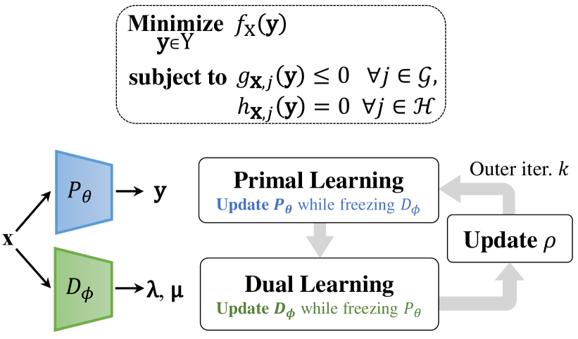
Figure 1: Schematic overview of PDL for training both primal and dual neural networks that output the optimal solutions of the constrained optimization problems.

A high-level overview of PDL is presented in Figure 1. It highlights that PDL alternates between primal learning, dual learning, and updating a penalty coefficient at each outer iteration. Given instances $\mathbf{x}$, the primal network $P_{\theta}$ outputs the primal solution estimates $\mathbf{y}$, i.e., $P_{\theta}(\mathbf{x})=\mathbf{y}$, whereas the dual network $D_{\phi}$ provides the dual solution estimates $\bm{\mu},\bm{\lambda}$ for equalities and inequalities, i.e., $D_{\phi}(\mathbf{x})=\{\bm{\mu},\bm{\lambda}\}$. The trainable parameters $\theta$ and $\phi$, associated with the primal and dual networks, respectively, are learned during training. Specifically, the primal learning updates $P_{\theta}$ while $D_{\phi}$ is frozen. Conversely, the dual learning updates $D_{\phi}$ while $P_{\theta}$ is frozen. Observe that PDL obtains both primal and dual estimates at inference time and is able to leverage any neural network architecture. The rest of this section provides all the details of PDL.

4.1 Primal Learning

The loss function for training the primal network is the objective function of the primal subproblem of the ALM: it combines a Lagrangian relaxation with a penalty on constraint violations. For each outer iteration $k$, the parameters $\theta$ of the primal network $P_{\theta}$ are trained while freezing $D_{\phi}$. The loss function of the primal training is given by

$$\mathcal{L}_{\text{p}}\left(\mathbf{y}\middle|\bm{\mu},\bm{\lambda}\right) =f_{\mathbf{x}}(\mathbf{y})\!+\!\bm{\mu}^{T}\mathbf{g}_{\mathbf{x}}(\mathbf{y})\!+\!\bm{\lambda}^{T}\mathbf{h}_{\mathbf{x}}(\mathbf{y})+$$ (5)

$$\frac{\rho}{2}\!\!\left(\sum_{j\in\mathcal{G}}\nu\left(g_{\mathbf{x},j}(\mathbf{y})\right)\!+\!\sum_{j\in\mathcal{H}}\nu\left(h_{\mathbf{x},j}(\mathbf{y})\right)\!\right),$$

where $\bm{\mu}$ and $\bm{\lambda}$ are the output of the frozen dual network $D_{\phi}$, i.e., the dual solution estimates for the inequality and equality constraints, respectively. Note that these dual estimates are instance-specific: for instance $\mathbf{x}$, the dual estimates are given by $D_{\phi}(\mathbf{x})$. The dual estimates are initialized to zero at the first outer iteration (which is readily achievable by imposing the initial weights and bias parameters of the final layer of $D_{\phi}$ to be zero). Observe that the initial dual estimate setting induces the primal loss function (5) is identical to the penalty loss (4). Also, this setting is mostly used in ALM itself. In Eq. (5), following the ALM, the violation functions for the inequality and equality constraints are defined as $\nu\left(g(\mathbf{y})\right)=\max\{g(\mathbf{y}),0\}^{2}$ and $\nu\left(h(\mathbf{y})\right)=h(\mathbf{y})^{2}$.

4.2 Dual Learning

The dual learning is particularly interesting. PDL does not store the dual estimates for all instances for ensuring efficiency and scalability. Instead, it trains the dual network $D_{\phi}$ to estimate them on a need basis. This training is again inspired by the ALM algorithm. At outer iteration $k$, the ALM updates the dual estimates using a proximal subgradient step:

$$\bm{\mu}_{k+1}\leftarrow\max\{\bm{\mu}_{k}+\rho\mathbf{g}(\mathbf{y}),0\},$$ (6)

$$\bm{\lambda}_{k+1}\leftarrow\bm{\lambda}_{k}+\rho\mathbf{h}(\mathbf{y}).$$

This update step suggests the targets for updating $D_{\phi}$. However, the dual training requires some care since the update rules refer both to the current estimates of the dual values, and to their new estimates. For this reason, at outer iteration $k$, the dual learning first copies the dual network into a “frozen” network $D_{\phi_{k}}$ that will provide the current estimates $\bm{\mu}_{k}$ and $\bm{\lambda}_{k}$. The dual learning can then update the dual network to yield a new estimate that is close to the RHS of the ALM dual update rule (Eq. (6)). Specifically, the dual network $D_{\phi}$ is trained by minimizing the following dual loss function:

$$\mathcal{L}_{\text{d}}\!\left(\!\bm{\mu},\bm{\lambda}\middle|\mathbf{y},\bm{\mu}_{k},\bm{\lambda}_{k}\!\right) =\!\left\lVert\bm{\mu}\!-\!\left(\max\{\bm{\mu}_{k}\!+\!\rho\mathbf{g}_{\mathbf{x}}(\mathbf{y}),0\}\right)\right\rVert$$ (7)

$$+\left\lVert\bm{\lambda}\!-\!\left(\!\bm{\lambda}_{k}\!+\!\rho\mathbf{h}_{\mathbf{x}}(\mathbf{y})\right)\right\rVert.$$

where $\bm{\mu}_{k}$ and $\bm{\lambda}_{k}$ are the outputs of the frozen network $D_{\phi_{k}}$ and $\mathbf{y}$ is the output of the primal network $P_{\theta}$. Note that the primal network $P_{\theta}$ is also frozen during the dual learning. Moreover, by minimizing the dual loss function (Eq. (7)), it is expected that, for each instance, the dual network yields the dual solution estimates that are close to those obtained in the ALM algorithm after applying the first-order proximal rule (Eq. (6)).

Algorithm 1 Primal-Dual Learning (PDL)

Parameter: Initial penalty coefficient $\rho$, Maximum outer iteration $K$, Maximum inner iteration $L$, Penalty coefficient updating multiplier $\alpha$, Violation tolerance $\tau$, Upper penalty coefficient safeguard $\rho_{\text{max}}$
Input: Training dataset $\mathcal{D}$
Output: learned primal and dual networks $P_{\theta}$, $D_{\phi}$

1:for $k\in\{1,\dots,K\}$ do

2:     for $l\in\{1,\dots,L\}$ do $\triangleright$ Primal Learning

3:         Update $P_{\theta}$ using $\nabla_{\theta}\mathcal{L}_{\text{p}}$ (See Eq. (5))

4:     end for

5:     Calculate $v_{k}$ as Eq. (8)

6:     Define $D_{\phi_{k}}$ by copying $D_{\phi}$

7:     for $l\in\{1,\dots,L\}$ do $\triangleright$ Dual Learning

8:         Update $D_{\phi}$ using $\nabla_{\phi}\mathcal{L}_{\text{d}}$ (See Eq. (7))

9:     end for

10:     Update $\rho$ with Eq. (9)

11:end for

12:return $\theta$ and $\phi$

4.3 Updating the Penalty Coefficient $\rho$

When constraint violations are severe, it is desirable to increase the penalty coefficient $\rho$, which is also used as a step size for updating the duals, in order to penalize violations more. PDL adopts the penalty coefficient updating rule from (Andreani et al. 2008) but slightly modifies it to consider all instances in the training dataset. At each outer iteration $k$, the maximum violation $v_{k}$ is calculated as

$$v_{k}=\max_{\mathbf{x}\sim\mathcal{D}}\left\{\max\{\left\lVert\mathbf{h}_{\mathbf{x}}(\mathbf{y})\right\rVert_{\infty},\left\lVert\bm{\sigma_{\mathbf{x}}(\mathbf{y})}\right\rVert_{\infty}\}\right\},$$ (8)

$$\text{where }\sigma_{\mathbf{x},j}(\mathbf{y})=\max\{g_{\mathbf{x},j}(\mathbf{y}),-\frac{\lambda_{k,j}}{\rho}\},\;\forall j\in\mathcal{G}$$

and $\mathcal{D}=\{\mathbf{x}^{(i)}\}_{i=1}^{N}$ is the training dataset. Informally speaking, the vector $\bm{\sigma}$ represents the infeasibility and complementarity for the inequality constraints (Andreani et al. 2008). At every outer iteration $k>1$, the penalty coefficient is increased when the maximum violation $v_{k}$ is greater than a tolerance value $\tau v_{k-1}$ as follows:

$$\rho\leftarrow\min\{\alpha\rho,\rho_{\text{max}}\}\;\text{if }v_{k}>\tau v_{k-1},$$ (9)

where $\tau\in(0,1)$ is a tolerance to determine the update of the penalty coefficient $\rho$, $\alpha>1$ is an update multiplier, and $\rho_{\text{max}}$ is the upper safeguard of $\rho$.

4.4 Training

The overall training procedure of PDL is detailed in Algorithm 1. The training alternates between the updates of the primal and dual networks. Unlike conventional training processes, the PDL training procedure contains outer and inner iterations. In an outer iteration, the two inner loops tackle the primal and dual learning subproblems. Each inner iteration samples a mini-batch and updates the trainable parameters ($\theta$ or $\phi$). Note that each outer iteration aims at estimating the primal and dual iteration points of the ALM algorithm. Eventually, these iteration points are expected to converge to the primal and dual solutions on the training instances and also provide the optimal solution estimates on unseen testing instances.

5 Experiments

This section demonstrates the effectiveness of PDL on a number of constrained optimization problems. The performance of PDL is measured by its optimality gaps and maximum constraint violations, which quantify both optimality and feasibility, respectively. PDL is compared to the supervised (SL) and self-supervised (SSL) baselines introduced in Section 3, i.e.,

• (Supervised) naïve MAE, naïve MSE: they respectively use the l₁-norm and the l₂-norm between the optimal solution estimates and the actual optimal solutions as loss functions (See Eq. (2)).

• (Supervised) MAE+Penalty, MSE+Penalty, LD: on top of naïve-MAE (or naïve-MSE), these methods add terms to penalize constraint violations (See Eq. (3)). For LD, l₁-norm is associated as used in (Chatzos et al. 2020).

• (Self-Supervised) Penalty this method uses a loss function that represents the average of the penalty functions given in Eq. (4) over the training instances.

• (Self-Supervised) DC3 The self-supervised method proposed by Donti, Rolnick, and Kolter (2021).

Note that DC3 is only tested on QP problems because the publicly available code is only applicable to those problems. Also, the penalty function in MAE(MSE)+Penalty(SL) and Penalty(SSL) uses absolute violations i.e., $\nu(a)=|a|$ for equalities and $\nu(a)=\max\{a,0\}$ for inequalities.

Note that PDL is generic and agnostic about the underlying neural network architectures. For comparison purposes with respect to the training methodology, the experimental evaluations are based on the simple fully-connected neural networks followed by ReLU activations. The implementation is based on PyTorch and the training was conducted using a Tesla RTX6000 GPU on a machine with Intel Xeon 2.7GHz. For training the models, the Adam optimizer (Kingma and Ba 2014) with the learning rate of $1\mathrm{e}{\textrm{-}4}$ was used. Other hyperparameters of PDL and the baselines were tuned using a grid search. The hyperparameter settings and architectural design are detailed in Appendix C.

5.1 Performance Results

Convex QP & Non-convex QP Variant

Method	Type	Obj.	Opt. Gap(%)	Max eq.	Max ineq.	Mean eq.	Mean ineq.
		convex QP (Eq. (10))
Optimizer(OSQP)		-15.047	-	0.000	0.001	0.000	0.000
Optimizer(ALM)		-15.046	0.003	0.000	0.000	0.000	0.000
PDL(ours)	SSL	-15.017(0.009)	0.176(0.054)	0.005(0.001)	0.001(0.000)	0.002(0.000)	0.000(0.000)
Penalty		-15.149(0.003)	0.680(0.017)	0.048(0.003)	0.030(0.003)	0.013(0.000)	0.004(0.001)
DC3		-14.112(0.015)	6.219(0.098)	0.000(0.000)	0.000(0.000)	0.000(0.000)	0.000(0.000)
Naïve MAE	SL	-15.051(0.003)	0.046(0.012)	0.025(0.002)	0.018(0.003)	0.008(0.001)	0.002(0.000)
Naïve MSE		-15.047(0.001)	0.122(0.025)	0.018(0.001)	0.023(0.004)	0.006(0.000)	0.003(0.001)
MAE+Penalty		-15.043(0.004)	0.093(0.013)	0.031(0.001)	0.016(0.001)	0.010(0.000)	0.002(0.000)
MSE+Penalty		-15.047(0.001)	0.059(0.004)	0.026(0.003)	0.016(0.001)	0.008(0.001)	0.002(0.000)
LD		-15.043(0.006)	0.093(0.015)	0.033(0.001)	0.016(0.001)	0.011(0.001)	0.002(0.000)
		non-convex QP variant (Eq. (11))
Optimizer(IPOPT)		-11.592	-	0.000	0.000	0.000	0.000
Optimizer(ALM)		-11.592	0.002	0.000	0.000	0.000	0.000
PDL (ours)	SSL	-11.552(0.006)	0.324(0.051)	0.004(0.001)	0.001(0.000)	0.001(0.000)	0.000(0.000)
Penalty		-11.654(0.002)	0.532(0.015)	0.042(0.002)	0.027(0.001)	0.011(0.000)	0.003(0.000)
DC3		-11.118(0.017)	4.103(0.151)	0.000(0.000)	0.000(0.000)	0.000(0.000)	0.000(0.000)
Naïve MAE	SL	-11.593(0.004)	0.044(0.021)	0.020(0.002)	0.022(0.006)	0.006(0.000)	0.001(0.001)
Naïve MSE		-11.593(0.002)	0.031(0.008)	0.017(0.000)	0.029(0.010)	0.005(0.000)	0.002(0.001)
MAE+Penalty		-11.591(0.004)	0.073(0.016)	0.033(0.001)	0.016(0.002)	0.010(0.000)	0.001(0.000)
MSE+Penalty		-11.593(0.001)	0.050(0.002)	0.023(0.002)	0.017(0.001)	0.007(0.001)	0.001(0.000)
LD		-11.593(0.005)	0.072(0.005)	0.032(0.001)	0.017(0.002)	0.010(0.000)	0.001(0.000)

Table 1: Performance results of the self-supervised (SSL) and supervised learning (SL) schemes for the convex QP problem (Top) and non-convex QP problem (Bottom) with $n=100$, $n_{\text{eq}}=n_{\text{ineq}}=50$ on 833 test instances. Std. dev. in parenthesis is evaluated across 5 independent runs. Underlined numbers denote poor results (opt. gap over 1% or max violation over 0.01).

This benchmark uses convex QP problems and their non-convex variants proposed for evaluating DC3 (Donti, Rolnick, and Kolter 2021). The experiments followed the same experimental protocol as in that paper. Given various $\mathbf{x}\in\mathbb{R}^{n_{\text{eq}}}$, the mathematical formulation for both cases reads as

$$\min_{\mathbf{y}\in\mathbb{R}^{n}}\frac{1}{2}\mathbf{y}^{T}\mathbf{Q}\mathbf{y}\!+\!\mathbf{r}^{T}\mathbf{y},\text{ s.t. }\mathbf{A}\mathbf{y}\!=\!\mathbf{x},\;\mathbf{G}\mathbf{y}\leq\mathbf{h},$$ (10)

$$\min_{\mathbf{y}\in\mathbb{R}^{n}}\frac{1}{2}\mathbf{y}^{T}\mathbf{Q}\mathbf{y}\!+\!\mathbf{r}^{T}\!\sin(\mathbf{y}),\text{ s.t. }\mathbf{A}\mathbf{y}\!=\!\mathbf{x},\,\mathbf{G}\mathbf{y}\leq\mathbf{h},$$ (11)

where $\mathbf{Q}\!\in\!\mathbb{R}^{n\times n}\!\succeq\!0$, $\mathbf{r}\!\in\!\mathbb{R}^{n}$, $\mathbf{A}\!\in\!\mathbb{R}^{n_{\text{eq}}\times n}$, $\mathbf{G}\!\in\!\mathbb{R}^{n_{\text{ineq}}\times n}$, and $\mathbf{h}\!\in\!\mathbb{R}^{n_{\text{ineq}}}$. $n$, $n_{\text{eq}}$, and $n_{\text{ineq}}$ denote the number of variables, equations, and inequality constraints, respectively. Eq. (11) is a non-convex variant of the convex QP (Eq. (10)) obtained by adding the element-wise sine operation. Overall, $10,000$ instances were generated and split into training/testing/validation datasets with the ratio of $10\!\!:\!\!1\!\!:\!\!1$.

Table 1 reports the performance results of the convex QP problem and its non-convex variant on the test instances. The first row for both tables reports the results of the ground truth, which is obtained by the optimization systems OSQP (Stellato et al. 2020) or IPOPT (Wächter and Biegler 2006). In addition, the results of the ALM are also reported: they show that the ALM converges well for these cases. The optimality gap in percentage is the average value of the optimality gaps over the test instances, i.e., $\frac{|f(\mathbf{y}^{*})-f(\mathbf{y})|}{|f(\mathbf{y}^{*})|}$. In the tables, columns ‘Max eq.’, ‘Max ineq.’, ‘Mean eq.’, ‘Mean ineq.’ represent the average violation of the maximum or average values for the equality or inequality constraints across the test instances. The performance of PDL, which is only slightly worse than ALM, is compelling when considering both optimality and feasibility. The baselines each present their own weakness. For example, supervised approaches tend to violate some constraints substantially, which can be marginally mitigated by adding penalty terms or employing the LD method. DC3, as it exploits the completion and correction steps, satisfies the constraints but presents significant optimality gaps. The superiority of PDL for these cases is even more compelling when testing with various configurations. Fig. 2 shows the optimality gaps and the maximum violations in various settings. Note that the PDL results are located close to the origin, meaning that it has negligible optimality gaps and constraint violations.

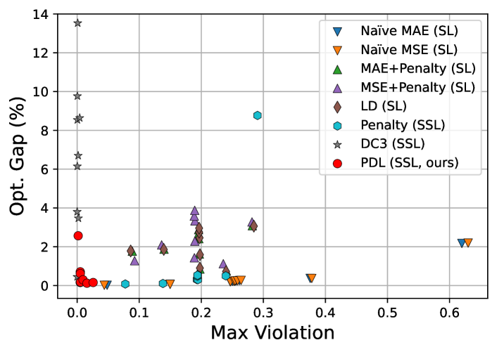
Figure 2: The optimality gaps (%) and maximum violations for various convex QP problems. Tested on 9 problem configurations using $n_{\text{eq}}\!=\!\{10,30,50,70,90\}$ and $n_{\text{ineq}}\!=\!50$, or $n_{\text{eq}}\!=\!50$ and $n_{\text{ineq}}\!=\!\{10,30,70,90\}$. The detailed results are described in Appendix D.

Quadratically Constrained Quadratic Program (QCQP)

Method	Obj.	Opt. Gap (%)		Time (s)
		mean	max
Opt.(Gurobi)	710.071	-	-	257.361
Opt.(CVXPY-QCQP)	1082.793	52.597	408.631	4.646
Opt.(ALM)	710.923	0.119	7.659	128.992
PDL(SSL, ours)	711.064	0.141	8.307	0.004
Penalty (SSL)	1295.388	82.555	109.406	0.004
Naïve MAE (SL)	716.132	0.834	67.051	0.004
Naïve MSE (SL)	716.695	0.911	85.073	0.004
MAE+Penalty (SL)	714.891	0.664	61.093	0.004
MSE+Penalty (SL)	717.869	1.072	80.577	0.004
LD (SL)	715.522	0.751	73.290	0.004

Table 2: Performance results for the QCQP problem (Eq. (12)) with $n=50$ and $n_{\text{aff}}=75$ on 1000 test instances. The best results are shown in bold.

QCQP is basically a non-convex problem in which both objective function and constraints are quadratic functions. This experiment considers a binary least-square minimization problem, which can be defined as

$$\min_{\mathbf{y}\in\mathbb{R}^{n}}\left(\mathbf{A}\mathbf{y}\!-\!\mathbf{x}\right)^{T}\!\!\left(\mathbf{A}\mathbf{y}\!-\!\mathbf{x}\right),\text{ s.t. }y_{i}^{2}=1,\;\forall i\!\in\!\{1,\dots,n\},$$ (12)

where $\mathbf{A}\in\mathbb{R}^{n_{\text{aff}}\times n}$ and $\mathbf{x}\in\mathbb{R}^{n_{\text{aff}}}$. Here, $n_{\text{aff}}$ is the dimension of the affine space. This problem can be formulated as a 0-1 integer programming problem as

$$\min_{\mathbf{y}\in\{-1,1\}^{n}}\left(\mathbf{A}\mathbf{y}-\mathbf{x}\right)^{T}\left(\mathbf{A}\mathbf{y}-\mathbf{x}\right).$$

Gurobi 9.5.2 (Gurobi Optimization, LLC 2022) was used as the optimization solver to produce the instance data for the supervised baselines, and also served as the reference for computing optimality gaps. In addition, CVXPY-QCQP (Park and Boyd 2017) was used as an alternative heuristic optimizer for additional comparisons. Since it is a heuristic method, CVXPY-QCQP tends to solve problems faster, but often converges to a suboptimal solution. The ALM is also included in the table for comparison. As it is a local search method and the local solution depends on the initial point, the table reports the best objective values obtained from 50 independent ALM runs with randomized initial points.

The overall results for $n=50$ and $n_{\text{aff}}=75$ are illustrated in Table 2. The supervised baselines are trained on 10,000 instances solved by Gurobi and the training instances for the self-supervised learning methods are generated on the fly during training. In this experiment, finding a feasible point is readily achievable as one can exploit a sigmoid function in the last layer of the neural network. Hence, the constraint violation results are not reported. Similar to the ALM and also inspired by the stochastic multi-start local search (Schoen 1991), 10 independent models with different seeds were built for each training method, and the reported results in the table are based on the best values among 10 inferences. The times reported in the table denote the inference times for training the learning schemes or the solving times for the optimization runs.

The results in Table 2 show that PDL is particularly effective. PDL is almost as accurate as the ALM in terms of optimality gaps, with a mean optimality gap of 0.14% and a maximum optimality gap of only 8.31% among 1,000 test instances. Note that the ALM method has a mean optimality gap of 0.12% and a maximum optimality gap of only 7.66% when solving (not learning) the 1,000 test instances. As a result, PDL provides about an order of magnitude improvement over the baselines. Moreover, PDL presents a speedup of around $64,340\times$ over Gurobi at the cost of a reasonable loss in optimality.

Method	case57		case118
	Gap(%)	Max viol.	Gap(%)	Max viol.
PDL (SSL, ours)	0.21(0.02)	0.01(0.00)	0.73(0.12)	0.04(0.01)
Penalty (SSL)	9.73(0.03)	0.03(0.00)	5.51(0.11)	0.05(0.00)
Naïve MAE (SL)	0.39(0.54)	0.09(0.06)	0.73(0.25)	0.35(0.13)
Naïve MSE (SL)	0.06(0.01)	0.06(0.03)	0.34(0.38)	0.21(0.12)
MAE+Penalty (SL)	0.37(0.52)	0.03(0.01)	0.91(0.86)	0.08(0.02)
MSE+Penalty (SL)	0.05(0.01)	0.02(0.00)	0.37(0.33)	0.05(0.01)
LD (SL)	0.33(0.45)	0.02(0.00)	0.70(0.60)	0.06(0.00)

Table 3: Performance results for the case56 and case118 AC-OPF problems. Std. dev. in parenthesis is evaluated across 5 independent runs. The detailed results on various AC-OPF problems are provided in Appendix D. The best values are in bold.

AC-Optimal Power Flow Problems

AC-optimal power flow (AC-OPF) is a fundamental building block for operating electrical power systems. AC-OPF determines the most economical setpoints for each generator, while satisfying the demand and physical/engineering constraints simultaneously. Different instances of an AC-OPF problem are given by the active and reactive power demands. The variables, which correspond to the output of the (primal) neural network, are the active and reactive power generations, the nodal voltage magnitudes, and the phase angles for all buses. The mathematical formulation of AC-OPF used in the paper is based on the formulation from PGLIB (Babaeinejadsarookolaee et al. 2019) and is described in Appendix B.

Table 3 reports the performance results of the case56 and case118 in PGLib (Babaeinejadsarookolaee et al. 2019). The results show that PDL produces competitive optimality gaps and maximum constraint violations, while supervised penalty approaches also show fine performances. However, for bulk power systems, where gathering the pre-solved instances is cumbersome, PDL may become a strong alternative to the supervised approaches for yielding real-time approximations of the solutions.

5.2 Training Time vs. Data Generation Time

Test Case	Training Time (s)		Pre-solved Training Set Generation Time (s)
	PDL (SSL)	LD (SL)
Convex QP	1558.5	1493.3	32.5
Nonconvex QP	1624.5	1550.4	630.1
AC-OPF(case57)	5932.5	8473.2	3690.2
AC-OPF(case118)	7605.1	9149.6	13120.3
QCQP	5553.2	3572.3	2573607.3 $\approx$ 715 hours

Table 4: The averaged elapsed time (s) for training PDL and the representative supervised learning baseline, LD (mid-column). The CPU time for gathering the pre-solved training instances (right-column).

Table 4 reports the training times for PDL, and shows that they are comparable to those of one of the supervised learning baselines, LD. Importantly, it also highlights a key benefit of PDL and self-supervised methods in general. Supervised learning schemes rely on pre-solved instances and may need to run an optimization solver on each input data. The QCQP problem required around $715$ hours of CPU time to collect the training dataset. In contrast, PDL, being self-supervised, does not need this step. This potential benefit may be important for training input/output mappings for large constrained optimization problems in a timely manner.

6 Conclusion

This paper presented PDL, a self-supervised Primal-Dual Learning scheme to learn the input/output mappings of constrained optimization problems. Contrary to supervised learning methods, PDL does not require a collection of pre-solved instances or an optimization solver. Instead, PDL tracks the iteration points of the ALM and jointly learns primal and dual networks that approximate primal and dual solution estimates. Moreover, being a primal-dual method, PDL features a loss function for primal training with instance-specific multipliers for its constraint terms. Experimental results on a number of constrained optimization problems highlight that PDL finds solutions with small optimality gaps and negligible constraint violations. Its approximations are remarkably close to the optimal solutions from the ALM, and PDL typically exhibits improved accuracy compared to supervised methods and primal self-supervised approaches.

PDL has also a number of additional benefits that remain to be explored. Being a primal-dual method, PDL provides dual approximations which can be useful for downstream tasks (e.g., approximating Locational Marginal Prices in power systems or prices in general). Dual solutions estimates can also be leveraged when learning is used for warm-starting an optimization or, more generally, speeding up an optimization solver by identifying the set of binding constraints. Finally, observe that PDL is generic with respect to the type of underlying primal and dual neural networks. The use of implicit layer to restore the feasibility of the primal solution estimates can be considered. Exploring more complex architectures for a variety of graph problems is also an interesting direction.

Appendix A Augmented Lagrangian Method

ALM (Bertsekas 2014; Hestenes 1969; Rockafellar 1974; Andreani et al. 2008; Wright, Nocedal et al. 1999) has been used for solving nonlinear constrained optimization problems. Suppose that we aim at solving the following constrained optimization problem:

$$P(\mathbf{y}): \operatornamewithlimits{\text{{minimize}}}_{\mathbf{y}\in\mathbf{Y}} f(\mathbf{y}),$$

subject to $$g_{j}(\mathbf{y})\leq 0,\;\forall j\in\mathcal{G},$$

$$h_{j}(\mathbf{y})=0,\;\forall j\in\mathcal{H}.$$

Given the Lagrangian multiplier estimates $\bm{\mu}\in\mathbb{R}^{|\mathcal{G}|}$, $\bm{\lambda}\in\mathbb{R}^{|\mathcal{H}|}$, the augmented Lagrangian function $L_{\rho}\!:\!\mathbb{R}^{n}\!\times\!\mathbb{R}_{+}^{|\mathcal{G}|}\!\times\!\mathbb{R}^{|\mathcal{H}|}\rightarrow\mathbb{R}$ is defined as follows:

$$L_{\rho}(\mathbf{y},\bm{\mu},\bm{\lambda})=f(\mathbf{y})+\bm{\mu}^{T}\mathbf{g}(\mathbf{y})+\bm{\lambda}^{T}\mathbf{h}(\mathbf{y})$$

$$+\frac{\rho}{2}\left(\left\lVert\max\{\mathbf{g}(\mathbf{y}),0\}\right\rVert_{2}^{2}+\left\lVert\mathbf{h}(\mathbf{y})\right\rVert_{2}^{2}\right),$$

where the max operator is applied element-wisely. At each iteration $k$, given the fixed Lagrangian multiplier estimates $\bm{\mu}_{k}$, $\bm{\lambda}_{k}$, it is aimed to solve the primal subproblem as

$$\mathbf{y}_{k}\in\operatorname*{arg\!\min}L_{\rho}(\mathbf{y},\bm{\mu}_{k},\bm{\lambda}_{k})$$

Then, using the proximal algorithm the Lagrangian multiplier estimates are updated as

$$\bm{\mu}_{k+1}\leftarrow\max\{\bm{\mu}_{k}+\rho\mathbf{g}(\mathbf{y}),0\}$$

$$\bm{\lambda}_{k+1}\leftarrow\bm{\lambda}_{k}+\rho\mathbf{h}(\mathbf{y}).$$

Also, the scaler $\rho>0$ could be increased when the violation gets worse. The $\rho$ updating rule comes from (Andreani et al. 2008), which considers both feasibility and complementarity. Specifically, the violation is first calculated for both equalities and inequalities as

$$v_{k}=\max\{\left\lVert\mathbf{h}_{\mathbf{x}}(\mathbf{y})\right\rVert_{\infty},\left\lVert\bm{\sigma_{\mathbf{x}}(\mathbf{y})}\right\rVert_{\infty}\}$$ (13)

$$\text{where }\sigma_{\mathbf{x},j}(\mathbf{y})=\max\{g_{\mathbf{x},j}(\mathbf{y}),-\frac{\lambda_{k,j}}{\rho}\},\;\forall j\in\mathcal{G}$$

Then, at every iteration $k>1$, the penalty coefficient $\rho$ is increased when the maximum violation $v_{k}$ is greater than a tolerance value $\tau v_{k-1}$ as

$$\rho\leftarrow\min\{\alpha\rho,\rho_{\text{max}}\}\;\text{if }v_{k}>\tau v_{k-1}$$ (14)

Overall, Algorithm 2 summarizes the procedure of the ALM. It is known that the primal and dual variables through the ALM converge to the KKT point at the limit. To show its performance, the ALM (Algorithm 2) is applied to the synthetic problems in the experiments including the QC problems and QCQP problem. In the implementation, the function minimize in Scipy 1.8.1 is used for solving the primal subproblem (corresponding to the line 3 in Algorithm 2). Specifically, a nonlinear conjugate gradient algorithm by Polak and Ribiere (Wright, Nocedal et al. 1999) involved in the function minimize is utilized with the terminating tolerance of $1\mathrm{e}{\textrm{-}4}$.

For the QC problems, $\alpha$ is set to $10$, initial penalty coefficient $\rho$ is set to $1.$, and $\tau=0.5$. Also the maximum outer iteration $K$ is set to $20$. The Lagrangian Multiplier estimates are initialized to zero. The initial primal point is randomly sampled from the uniform distribution over $[-1,1]$.

For the QCQP problem, since it is highly non-convex, stochastic multi-start local search (Schoen 1991) is applied. Specifically, 50 independent runs are conducted and the best objective value is chosen. To do so, the initial primal point is also i.i.d. sampled from the uniform distribution over $[-2,2]$. Also the initial Lagrangian multiplier estimates $\bm{\lambda}$ are i.i.d sampled from the uniform distribution over $[-2,2]$. (Note that $\bm{\mu}$ is not used in this problem.) The parameters are set differently; $\alpha=1.2$, $\rho=0.1$, $\tau=0.5$. The maximum outer iteration $K$ is set to $50$.

Algorithm 2 Augmented Lagrangian Method (ALM)

1:Initialize $\bm{\mu}_{1}$, $\bm{\lambda}_{1}$, and $\rho$

2:for $k\in\{1,\dots,K\}$ do

3:     Solve $\mathbf{y}_{k}\in\operatorname*{arg\!\min}_{\mathbf{y}}L_{\rho}(\mathbf{y},\bm{\mu}_{k},\bm{\lambda}_{k})$

4:     $\displaystyle\bm{\mu}_{k+1}\leftarrow\max\{\bm{\mu}_{k}+\rho\mathbf{g}(\mathbf{y}),0\}$

5:     $\bm{\lambda}_{k+1}\leftarrow\bm{\lambda}_{k}+\rho\mathbf{h}(\mathbf{y})$

6:     Calculate $v_{k}$ using Eq. (13)

7:     if $v_{k}<\epsilon$ then

8:         Converged

9:     end if

10:     Update $\rho$ using Eq. (14)

11:end for

Appendix B Details on AC-OPF Problem

The Optimal Power Flow (OPF) determines the most economic generator setpoints that satisfy the load demands as well as physical constraints simultaneously in a power network. The power network can be represented as a graph $(\mathcal{N},\mathcal{E})$ where $\mathcal{N}$ is the nodes representing the set of bus IDs, which also contains generators and load units, and $\mathcal{E}$ represents the set of transmission line IDs between buses. $(lij)\in\mathcal{E}$ where $l$ is a branch ID connected from node $i$ to $j$. The set $\mathcal{E}^{R}$ captures the reversed orientation of $\mathcal{E}$, i.e., $(lji)\in\mathcal{E}^{R}$. Also, two subsets of $\mathcal{N}$ are defined; the set of generator IDs $\mathcal{G}$ and set of load demand IDs $\mathcal{L}$.

Overall, the AC-OPF formulation is detailed in Model (1). This AC-OPF problem is a nonlinear and non-convex program over complex numbers and variables. AC power generation $S^{g}$ is a complex number of which a real part $p^{g}$ is an active power generation and an imaginary part $q^{g}$ is a reactive power generation per each generator. Also, at each bus, AC voltage $V$ can be separated into a voltage magnitude $v$ and voltage angle $\theta$.

The objective (15) is to minimize the sum of the quadratic costs of the active power generations. At the reference bus $r$, the voltage angle is set to zero as defined in constraint (16). Maximum and minimum active and reactive power generation at each generation unit are captured in constraints (17a), (17b). Similarly, the bounds of the voltage magnitude are set in constraint (18). Constraint (19a), (19b) represent the power flow at each branch that is governed by Ohm’s law. Constraint (20) ensures that at each bus the power balance should be maintained. Constraints (21), (22) capture the branch thermal limit and branch voltage angle difference limit, respectively.

Model 1 AC-Optimal Power Flow (AC-OPF) Problem

Sets:

$$\text{bus IDs }\mathcal{N}$$

$$\text{generator IDs }\mathcal{G}$$

$$\text{load demand IDs }\mathcal{L}$$

$$\text{transmission line IDs }\mathcal{E}$$

Parameters:

$$\text{AC power demand }S_{i}^{d}=p_{i}^{d}+jq_{i}^{d} \forall i\in\mathcal{L}$$

$$\text{cost coefficients }c_{2i},c_{1i},c_{0i} \forall i\in\mathcal{G}$$

$$\text{reference bus ID }r\in\mathcal{N}$$

$$\text{generation bounds }\underline{p}_{i}^{g},\overline{p}_{i}^{g},\underline{q}_{i}^{g},\overline{q}_{i}^{g} \forall i\in\mathcal{G}$$

$$\text{series admittance }Y_{l} \forall(lij)\in\mathcal{E}$$

$$\text{line charging susceptance }b_{l}^{c} \forall(lij)\in\mathcal{E}$$

$$\text{transformer parameter }T_{l} \forall(lij)\in\mathcal{E}$$

$$\text{bus shunt admittance }Y_{i}^{s} \forall i\in\mathcal{N}$$

$$\text{thermal bound }\bar{s}_{l} \forall(lij)\in\mathcal{E}$$

$$\text{angle difference bounds }\underline{\Delta\theta}_{l},\overline{\Delta\theta}_{l} \forall(lij)\in\mathcal{E}$$

Variables:

$$\text{AC power generation }S^{g}_{i}=p_{i}^{g}+jq_{i}^{g} \forall i\in\mathcal{G}$$

$$\text{AC voltage }V_{i}=v_{i}\angle\theta_{i} \forall i\in\mathcal{N}$$

$$\text{AC branch power flow }S_{lij} \forall(lij)\!\in\!\mathcal{E}\!\cup\!\mathcal{E}^{R}$$

Objective Function:

$$\min\sum_{i\in\mathcal{G}}{c_{2i}(p_{i}^{g})^{2}+c_{1i}p_{i}^{g}+c_{0i}},$$ (15)

Constraints:

$$\theta_{r}=0,$$ (16)

$$\underline{p}_{i}^{g}\leq p_{i}^{g}\leq\overline{p}_{i}^{g},\; \forall i\in\mathcal{G}$$ (17a)

$$\underline{q}_{i}^{g}\leq q_{i}^{g}\leq\overline{q}_{i}^{g},\; \forall i\in\mathcal{G}$$ (17b)

$$\underline{v}_{i}\leq v_{i}\leq\overline{v}_{i}, \forall i\in\mathcal{N}$$ (18)

$$S_{lij}\!=\!\left(Y_{l}^{*}\!-\!j\frac{b_{l}^{c}}{2}\right)\frac{v_{i}^{2}}{|T_{l}|^{2}}-Y_{l}^{*}\frac{V_{i}V_{j}^{*}}{T_{l}} \forall(lij)\!\in\!\mathcal{E}$$ (19a)

$$S_{lji}\!=\!\left(Y_{l}^{*}\!-\!j\frac{b_{l}^{c}}{2}\right)v_{i}^{2}-Y_{l}^{*}\frac{V_{i}^{*}V_{j}}{T_{l}^{*}} \forall(lji)\!\in\!\mathcal{E}^{R}$$ (19b)

$$\sum_{k\in\mathcal{G}_{i}}S_{k}^{g}\!\!-\!\!S_{i}^{d}\!\!-\!\!Y_{i}^{s}|V_{i}|^{2}=\!\!\!\!\!\!\!\!\sum_{(lij)\in\mathcal{E}\cup\mathcal{E}^{R}}\!\!\!\!S_{lij} \forall i\in\mathcal{N}$$ (20)

$$|S_{lij}|\leq\bar{s}_{l} \forall(lij)\!\in\!\mathcal{E}\!\cup\!\mathcal{E}^{R}$$ (21)

$$\underline{\Delta\theta}_{l}\leq\theta_{i}-\theta_{j}\leq\overline{\Delta\theta}_{l} \forall(lij)\!\in\!\mathcal{E}$$ (22)

Appendix C Details on Experiment Settings

C.1 Data Generation

QP cases

As the protocol of the experiments for the convex QP and its non-convex variant follows that of DC3 (Donti, Rolnick, and Kolter 2021), the overall data generation process is exactly the same as that in the paper. For the sake of completeness, the general process of generating the data instances is presented as follows. The quadratic matrix $\mathbf{Q}$ involved in the objective function (both Eq. (10) and Eq. (11)) is assumed to be diagonal and positive semi-definite, which is ensured by setting the all diagonal entries are i.i.d. sampled from the uniform distribution on $[0.,1.]$. Also, the elements in matrices $\mathbf{A}$ and $\mathbf{G}$ are i.i.d. sampled from the uniform distribution on $[0.,1.]$. The matrix $\mathbf{h}$ is determined to be $\mathbf{h}=\sum_{j}{|\mathbf{G}\mathbf{A}^{+}|_{ij}}$ where $\mathbf{A}^{+}$ is the Moore-Penrose pseudo-inverse of $\mathbf{A}$, i.e. $\mathbf{A}\mathbf{A}^{+}=\mathbf{I}$. Then this ensures that the problem is always feasible with the variables satisfying $\mathbf{A}\mathbf{y}=\mathbf{x}$ because

$$\mathbf{G}\mathbf{y}\leq\mathbf{h}\Rightarrow\mathbf{G}\mathbf{A}^{+}\mathbf{x}\leq\sum_{j}{|\mathbf{G}\mathbf{A}^{+}|_{ij}}$$ (23)

which holds for every $\mathbf{x}$ with $x_{j}\in[-1,1]$ for all $j$. Thus, $\mathbf{x}$ is i.i.d. sampled from the uniform distribution $\mathcal{U}(-1,1)$ to satisfy the inequality constraints.

For training the supervised baselines on the convex cases, OSQC 0.6.2 is utilized. Also, for the non-convex cases, IPOPT (cyipopt 1.1.0) is used. For both optimizers, the default settings are used when gathering the data instances.

QCQP case

The each element of input $\mathbf{x}\in\mathbb{R}^{n_{\text{aff}}}$ is i.i.d. sampled from the uniform distribution $\mathcal{U}(-1,1)$. Also, Ensure that $\mathbf{A}\in\mathbb{R}^{n_{\text{aff}}\times n}$ is full column rank in which all the elements are i.i.d. sampled from the standard normal distribution. The self-supervised baseline and PDL use the training data instances generated on the fly, whereas the supervised baselines used $10000$ pre-solved instances of $\mathbf{x}$ and $\mathbf{y}$ pairs for training. At inference time, 1000 instances that are unseen during training are used for reporting the performance. Gurobi 9.5.2 is used for generating the pre-solved instances for testing as well as for training the supervised baselines.

AC-OPF cases

Test case	dim($\mathbf{x}$)	dim($\mathbf{y}$)	$n_{\text{ineq}}$	$n_{\text{eq}}$	$|\mathcal{N}|$	$|\mathcal{G}|$	$|\mathcal{L}|$	$|\mathcal{E}|$
case57_ieee	84	151	160	114	57	7	42	80
case118_ieee	198	412	372	236	118	54	99	186

Table 5: Specifications of the AC-OPF test cases.

As shown in Table 5, two test cases varying the number of buses, generators, and load units are considered.

For the AC-OPF test cases, the load demands, $p^{d}$, $q^{d}$, for all load units $\mathcal{L}$ are perturbed to augment the problem data instances. In PGLIB (Babaeinejadsarookolaee et al. 2019), the original (reference) load demands is specified. Let us denote the concatenated vector of the original active and reactive load demands as $\hat{\mathbf{x}}$ then the perturbed input $\mathbf{x}$ is realized by multiplying so-called load factor $\mathbf{f}$ as

$$\mathbf{x}=\mathbf{f}\odot\hat{\mathbf{x}},$$ (24)

where $\odot$ is the element-wise multiplication. The load factor $\mathbf{f}$ is sampled from the truncated multivariate Gaussian distribution following (Zamzam and Baker 2020) as

$$\mathbf{f}\sim\mathcal{T}\mathcal{N}\left(\mathbf{1},\Sigma,(1-\mu)\mathbf{1},(1+\mu)\mathbf{1}\right),$$ (25)

where the first argument is the mean, $\Sigma$ denotes the covariance matrix, and the other two are lower and upper limits for truncation. In our experiment, we set $\mu$ to $0.3$ and the covariance matrix $\Sigma$ to the correlated covariance with the correlation parameter of $0.8$.

Totally 30000 instances are generated and separated into train/valid/test datasets with a ratio of 10:1:1. The optimizer is included in PowerModels.jl (Coffrin et al. 2018), which is IPOPT 3.14.4 in general with MUMPS 5.4.1 as a linear solver. We have used the default settings for experiments.

C.2 Architecture Design and Training Procedure

QC cases

For both the primal and dual nets in PDL and for other baselines, MLP with 2 hidden layers of size 500 is used. Also, a ReLU activation is attached to each layer. Batch normalization and Dropout layers are excluded because it is found that adding those degrades the performance. But for DC3, those are not excluded as used in the original work. For the baselines, the number of maximum epochs is set to $10000$, which is equivalent to using the maximum outer iteration of $K=10$ with the $500$ inner epochs (for each primal or dual learning) for PDL.

QCQP case

The architectural design for PDL and the baselines is the same as it is for QC cases except that the Sigmoid activation is attached to the final layer to yield a binary decision, which is, in turn, scaled to $\left[-1,1\right]$. The number of iterations for the self-supervised penalty method is set to $100000$ and equivalently, for the supervised baselines, the number of epochs is set to $2000$. Also, for PDL, the number of outer iterations is set to $10$ and $5000$ inner iterations for both primal and dual learning are used.

AC-OPF cases

The input and output of the (primal) neural network are defined as below:

$\;\;-$ Input

AC power demands $p_{i}^{d},q_{i}^{d}$, $\forall i\in\mathcal{N}$

$\;\;-$ Output

AC power generations $p_{i}^{g},q_{i}^{g}$, $\forall i\in\mathcal{G}$
AC voltage magnitudes $v_{i}$, $\forall i\in\mathcal{N}$
AC voltage angle difference $\theta_{i}-\theta_{j}$, $\forall(lij)\in\mathcal{E}$

The AC power demands are all concatenated to serve an input $\mathbf{x}$. The hidden representation is embedded using 2 layered MLPs. Each layer has $1.2\times$dim($\mathbf{y}$) nodes. Then the hidden representation is served as an input of the ‘individual’ net for outputting the four individual estimates; active, reactive generations, and the voltage magnitude and angle difference. All four individual nets have one hidden layer with nodes of the same size as the output dimension for each output. Also, ReLU activations are followed to all fully-connected layers. Since the AC power generations and voltage magnitudes have bound constraints, the Hardsigmoid activation, which outputs a value in a range of $[0.,1.]$, is attached to the last layer. Then, using the bound limits, the convex combination of both bounds using the output of the individual model would be the eventual output of the neural net. Consequently, the bound constraints Eq. (17a), (17b), (18), and (22) in AC-OPF problem (Model (1)) are always satisfied without having the explicit penalty functions. Once the outputs from the four individual neural nets are furnished, the power flows $S_{lij}$ can be directly calculated from Ohm’s law (Eq. (19a) and (19b) in AC-OPF problem (Model (1))).

For PDL, the number of outer iterations is set to $10$ and the inner epochs are set to $250$ for both learning subproblems. For the self-supervised and supervised baseline, the number of epochs is set to $5000$.

C.3 Hyperparameters

For all cases and methods, the number of instances in the minibatch $|\mathcal{B}|$ is set to $200$. Also, the training process is performed using Adam optimizer (Kingma and Ba 2014) with a learning rate of $1\mathrm{e}{\textrm{-}4}$. For PDL, the learning rate is decayed by $0.99$ when the validation loss is bigger than the best validation loss in the primal or dual learning procedure. For QCQP cases, validation loss is evaluated every 500 inner iterations to determine the adjustment of the learning rate whereas for the other problem cases, it is evaluated every epoch. Since this learning rate decay is not beneficial to the baselines empirically (it leads to premature convergence in most cases), it is not applied to those.

QP cases

For DC3, all the hyperparameters suggested by the original work (Donti, Rolnick, and Kolter 2021) are used. The hyperparameters for PDL and other baselines are tuned using the convex case through the grid search and those resultant combinations are also applied to the non-convex QP variants. For all methods, here is the list of the candidate hyperparameters where the chosen hyperparameters are in bold.

• PDL

  • $\tau$: $0.5$, $0.6$, $0.7$, $\mathbf{0.8}$, $0.9$

  • $\rho$: $0.1$, $\mathbf{0.5}$, $1.$, $10.$

  • $\rho_{\text{max}}$: $1000.$, $\mathbf{5000.}$, $10000.$, $50000.$

  • $\alpha$: $1.$, $1.5$, $2.$, $5.$, $\mathbf{10.}$

• MAE+Penalty, MSE+Penalty, and LD (SL)

  • $\rho_{g}$: $0.1$, $0.5$, $1.$, $\mathbf{5.}$, $10.$, $50.$

  • $\rho_{h}$: $0.1$, $0.5$, $1.$, $\mathbf{5.}$, $10.$, $50.$

  • LD updating epochs: $\mathbf{50.}$, $100$, $200$, $300$, $500$, $1000$

  • LD step size: $1\mathrm{e}{0}$, $1\mathrm{e}{\textrm{-}1}$, $1e{\textrm{-}2}$, $\mathbf{1\mathrm{e}{\textrm{-}3}}$, $1\mathrm{e}{\textrm{-}4}$

• Penalty (SSL)

  • $\rho_{g}$: $0.1$, $0.5$, $1.$, $\mathbf{5.}$, $10.$, $50.$, $100.$

  • $\rho_{h}$: $0.1$, $0.5$, $1.$, $\mathbf{5.}$, $10.$, $50.$, $100.$

QCQP case

All experiment settings and the architectural design for all baselines and the PDL are the same as those for the QP problems. Hyperparameters are as follows:

• PDL

  • $\tau$: $0.5$, $0.6$, $0.7$, $\mathbf{0.8}$, $0.9$

  • $\rho$: $0.1$, $0.5$, $\mathbf{1.}$, $10.$

  • $\rho_{\text{max}}$: $1000.$, $5000.$, $\mathbf{10000.}$, $50000.$

  • $\alpha$: $1.$, $\mathbf{1.5}$, $2.$, $5.$, $10.$

• MAE+Penalty and LD (SL)

  • $\rho_{g}$: $\mathbf{0.1}$, $0.5$, $1.$, $5.$, $10.$, $50.$

  • $\rho_{h}$: $\mathbf{0.1}$, $0.5$, $1.$, $5.$, $10.$, $50.$

  • LD updating epochs: $\mathbf{50}$, $100$, $200$, $300$, $500$, $1000$

  • LD step size: $\mathbf{1\mathrm{e}{0}}$, $1\mathrm{e}{\textrm{-}1}$, $1e{\textrm{-}2}$, $1\mathrm{e}{\textrm{-}3}$, $1\mathrm{e}{\textrm{-}4}$

• MSE+Penalty (SL)

  • $\rho_{g}$: $0.1$, $0.5$, $\mathbf{1.}$, $5.$, $10.$, $50.$

  • $\rho_{h}$: $0.1$, $0.5$, $\mathbf{1.}$, $5.$, $10.$, $50.$

• Penalty (SSL)

  • $\rho_{g}$: $0.1$, $0.5$, $1.$, $5.$, $10.$, $50.$, $\mathbf{100.}$

  • $\rho_{h}$: $0.1$, $0.5$, $1.$, $5.$, $10.$, $50.$, $\mathbf{100.}$

AC-OPF cases

Hyperparameter tuning for AC-OPF cases were conducted on case118, then applied the same hyperparameter combination to the case57 problem.

• PDL

  • $\tau$: $0.5$, $0.6$, $0.7$, $\mathbf{0.8}$, $0.9$

  • $\rho$: $0.1$, $0.5$, $\mathbf{1.}$, $10.$

  • $\rho_{\text{max}}$: $1000.$, $5000.$, $\mathbf{10000.}$, $50000.$

  • $\alpha$: $1.$, $1.5$, $\mathbf{2.}$, $5.$, $10.$

• MAE+Penalty, MSE+Penalty, and LD (SL)

  • $\rho_{g}$: $0.1$, $0.5$, $\mathbf{1.}$, $5.$, $10.$, $50.$

  • $\rho_{h}$: $0.1$, $0.5$, $\mathbf{1.}$, $5.$, $10.$, $50.$

  • LD updating epochs: $\mathbf{50.}$, $100$, $200$, $300$, $500$, $1000$

  • LD step size: $\mathbf{1\mathrm{e}{0}}$, $1\mathrm{e}{\textrm{-}1}$, $1e{\textrm{-}2}$, $1\mathrm{e}{\textrm{-}3}$, $1\mathrm{e}{\textrm{-}4}$

• Penalty (SSL)

  • $\rho_{g}$: $0.1$, $0.5$, $\mathbf{1.}$, $5.$, $10.$, $50.$, $100.$

  • $\rho_{h}$: $0.1$, $0.5$, $\mathbf{1.}$, $5.$, $10.$, $50.$, $100.$

Appendix D Additional Experiment Results

D.1 Training Time vs. Data Generation Time

Test Case	PDL (SSL)	Penalty (SSL)	DC3 (SSL)	Naïve MAE (SL)	Naïve MSE (SL)	MAE+Penalty (SL)	MSE+Penalty (SL)	LD (SL)
convex QP	1558.45	1516.40	8099.22	1338.56	1329.03	1406.61	1417.23	1493.29
non-convex QP variant	1624.46	1576.17	6133.50	1382.40	1372.23	1460.79	1474.86	1550.42
QCQP	555.32	559.99	-	321.22	322.44	344.73	344.94	357.23
AC-OPF(case57)	5932.47	8173.71	-	7058.20	7038.17	8471.24	8528.35	8473.21
AC-OPF(case118)	7605.10	9433.96	-	7628.11	7598.09	9147.71	9179.24	9149.57

Table 6: Averaged training GPU time (s) of the approaches for the various test cases.

Test Case	Instance Solving Time (s)	# Training Instances	Pre-solved Training Set Generation Time (s)
convex QP (OSQP)	0.0039	8334	32.50
non-convex QP variant (IPOPT)	0.0756	8334	630.05
AC-OPF (case57)	0.1476	25000	3690.21
AC-OPF (case118)	0.5248	25000	13120.30
QCQP (Gurobi)	257.3607	10000	2573607.34

Table 7: Averaged CPU time (s) for solving a problem instance. Considering the number of training instances, the CPU time for arranging the training dataset for the supervised learning schemes is calculated by default.

Typically, DC3 takes a longer time to train because it involves the implicit differentiation (in the completion steps) to satisfy the equalities. The difference in time taken for training between PDL and Penalty (SSL) comes from the architectural design; PDL uses two independent neural networks and the number of hidden nodes varies depending on the dimension of the output (the dimension of the primal or dual solution space). When comparing the naïve SL methods with the penalty SL methods, it is obvious that the penalty ones take a longer time. This is because it involves the back-propagation through the constraint functions.

D.2 Additional QP Results

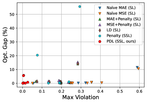
Figure 3: The optimality gaps (%) and maximum violations for various non-convex QP variants. The maximum violation means the maximum value between the equality and inequality constraint maximum violations. Tested on various problems generated using $n_{\text{eq}}\!=\!\{10,30,50,70,90\}$ and $n_{\text{ineq}}\!=\!50$, or $n_{\text{eq}}\!=\!50$ and $n_{\text{ineq}}\!=\!\{10,30,70,90\}$. DC3 is excluded due to its poor performance.

Method	$n_{\text{eq}}$	$10$	$30$	$70$	$90$	$50$	$50$	$50$	$50$	$10$	$30$	$70$	$90$	$50$	$50$	$50$	$50$
	$n_{\text{ineq}}$	$50$	$50$	$50$	$50$	$10$	$30$	$70$	$90$	$50$	$50$	$50$	$50$	$10$	$30$	$70$	$90$
		convex QP problems								non-convex QP problems
Optimizer(OSQP or IPOPT)	Obj.	-27.26	-23.13	-14.80	-4.79	-17.34	-16.33	-14.61	-14.26	-18.57	-16.92	-7.13	-1.33	-18.11	-12.30	-13.32	-8.64
PDL (SSL, ours)	Obj.	-26.55	-23.06	-14.78	-4.80	-17.31	-16.30	-14.50	-14.17	-18.56	-15.96	-7.12	-1.33	-18.07	-11.57	-13.29	-8.61
	Opt. Gap(%)	2.57	0.3	0.12	0.16	0.16	0.17	0.71	0.62	0.04	5.54	0.11	0.74	0.13	5.71	0.19	0.28
	Max eq.	0.00	0.01	0.02	0.03	0.01	0.00	0.00	0.01	0.00	0.00	0.01	0.03	0.00	0.01	0.00	0.00
	Max ineq.	0.00	0.00	0.00	0.00	0.00	0.00	0.00	0.00	0.00	0.00	0.00	0.00	0.00	0.00	0.00	0.00
Penalty (SSL)	Obj.	-27.28	-23.11	-14.76	-5.30	-17.39	-16.32	-14.52	-14.18	-14.78	-16.91	-7.23	-2.04	-18.09	-12.19	-13.32	-8.65
	Opt. Gap(%)	0.08	0.11	0.50	8.77	0.31	0.30	0.54	0.53	20.38	0.12	1.03	55.60	0.18	0.54	0.23	0.37
	Max eq.	0.08	0.14	0.24	0.29	0.19	0.19	0.19	0.19	0.08	0.13	0.24	0.29	0.19	0.19	0.19	0.19
	Max ineq.	0.05	0.04	0.00	0.00	0.02	0.02	0.02	0.02	0.03	0.02	0.00	0.00	0.00	0.02	0.02	0.02
DC3 (SSL)	Obj.	-26.30	-21.11	-14.23	-4.76	-16.14	-14.90	-12.60	-12.85	-13.83	-14.57	4e33	-1.25	-17.83	-10.97	-12.30	-8.20
	Opt. Gap(%)	3.47	8.64	3.80	0.45	6.70	8.54	13.53	9.77	25.53	13.55	4e34	3.67	1.48	10.45	7.49	5.00
	Max eq.	0.00	0.00	0.00	0.00	0.00	0.00	0.00	0.00	0.00	0.00	2e2	0.00	0.00	0.00	0.00	0.00
	Max ineq.	0.00	0.00	0.00	0.00	0.00	0.00	0.00	0.00	0.00	0.01	2e17	0.00	0.00	0.01	0.00	0.00
Naïve MAE (SL)	Obj.	-27.25	-23.14	-14.84	-4.89	-17.35	-16.35	-14.63	-14.29	-18.57	-16.93	-7.18	-1.48	-18.13	-12.32	-13.35	-8.66
	Opt. Gap(%)	0.02	0.06	0.37	2.17	0.20	0.22	0.24	0.26	0.03	0.10	0.72	11.50	0.15	0.29	0.21	0.31
	Max eq.	0.05	0.15	0.38	0.62	0.25	0.25	0.26	0.26	0.06	0.19	0.35	0.59	0.29	0.32	0.25	0.24
	Max ineq.	0.01	0.01	0.03	0.00	0.01	0.03	0.05	0.06	0.01	0.05	0.01	0.00	0.02	0.07	0.04	0.04
Naïve MSE (SL)	Obj.	-27.25	-23.14	-14.84	-4.89	-17.35	-16.35	-14.63	-14.29	-18.57	-16.93	-7.18	-1.46	-18.13	-12.31	-13.34	-8.66
	Opt. Gap(%)	0.01	0.06	0.37	2.19	0.19	0.22	0.24	0.26	0.02	0.13	0.69	10.50	0.15	0.33	0.20	0.30
	Max eq.	0.04	0.15	0.38	0.63	0.25	0.25	0.26	0.26	0.05	0.26	0.35	0.60	0.33	0.41	0.25	0.24
	Max ineq.	0.01	0.01	0.03	0.00	0.01	0.02	0.05	0.06	0.01	0.07	0.00	0.00	0.04	0.07	0.04	0.04
MAE+Penalty (SL)	Obj.	-26.77	-22.69	-14.66	-4.99	-17.16	-16.04	-14.18	-13.82	-18.31	-16.72	-7.17	-1.52	-18.05	-12.13	-13.24	-8.54
	Opt. Gap(%)	1.77	1.87	0.75	3.08	0.85	1.62	2.69	2.88	1.37	1.16	0.70	14.12	0.24	1.07	0.47	0.97
	Max eq.	0.09	0.14	0.24	0.28	0.20	0.20	0.20	0.20	0.07	0.14	0.24	0.28	0.20	0.20	0.20	0.19
	Max ineq.	0.00	0.00	0.00	0.00	0.00	0.00	0.00	0.00	0.00	0.00	0.00	0.00	0.00	0.00	0.00	0.00
MSE+Penalty (SL)	Obj.	-26.91	-22.63	-14.59	-5.01	-17.07	-15.93	-14.05	-13.67	-18.31	-16.64	-7.14	-1.53	-18.01	-12.08	-13.17	-8.44
	Opt. Gap(%)	1.28	2.10	1.13	3.28	1.43	2.29	3.58	3.88	1.36	1.59	0.67	15.37	0.42	1.55	0.92	1.99
	Max eq.	0.09	0.14	0.24	0.28	0.19	0.19	0.19	0.19	0.07	0.13	0.23	0.28	0.19	0.19	0.19	0.19
	Max ineq.	0.00	0.00	0.00	0.00	0.00	0.00	0.00	0.00	0.00	0.00	0.00	0.00	0.00	0.00	0.00	0.00
LD (SL)	Obj.	-26.77	-22.69	-14.67	-4.99	-17.15	-16.05	-14.17	-13.81	-18.31	-16.71	-7.17	-1.51	-18.05	-12.13	-13.24	-8.54
	Opt. Gap(%)	1.78	1.86	0.72	3.06	0.90	1.59	2.75	2.96	1.39	1.18	0.69	14.16	0.26	1.09	0.49	0.96
	Max eq.	0.09	0.14	0.24	0.28	0.20	0.20	0.20	0.20	0.07	0.14	0.24	0.28	0.20	0.20	0.20	0.19
	Max ineq.	0.00	0.00	0.00	0.00	0.00	0.00	0.00	0.00	0.00	0.00	0.00	0.00	0.00	0.00	0.00	0.00

Table 8: Performance results of various convex and non-convex QP problems.

We exclude DC3 results from Figure 3 for the non-convex QP variant cases because it is unstable in some cases. The detailed performance values can be found in Table 8.

D.3 Detailed QCQP results

Method	Obj.	Opt Gap (%)				Time (s)
		min	mean	median	max
Optimizer(Gurobi)	710.071	-	-	-	-	257.361
Optimizer(CVXPY-QCQP)	1082.793	5.583	52.597	50.589	408.631	4.646
Optimizer(ALM)	710.923	0.000	0.119	0.000	7.659	128.992
PDL(SSL, ours)	711.064(0.049)	0.000(0.000)	0.141(0.007)	0.000(0.000)	8.307(0.000)	0.004(0.000)
Penalty (SSL)	1295.388(9.994)	62.211(2.179)	82.555(1.406)	82.145(1.418)	109.406(3.712)	0.004(0.000)
Naïve MAE (SL)	716.132(0.544)	0.000(0.000)	0.834(0.075)	0.000(0.000)	67.051(14.249)	0.004(0.000)
Naïve MSE (SL)	716.695(1.223)	0.000(0.000)	0.911(0.168)	0.000(0.000)	85.073(24.454)	0.004(0.000)
MAE+Penalty (SL)	714.891(0.604)	0.000(0.000)	0.664(0.082)	0.000(0.000)	61.093(2.492)	0.004(0.000)
MSE+Penalty (SL)	717.869(0.945)	0.000(0.000)	1.072(0.130)	0.000(0.000)	80.577(8.594)	0.004(0.000)
LD (SL)	715.522(0.696)	0.000(0.000)	0.751(0.095)	0.000(0.000)	73.290(10.249)	0.004(0.000)

Table 9: Detailed performance results for QCQP problem (Eq. (12)) with $n=50$ and $n_{\text{aff}}=75$ on 1000 test instances. The best results are shown in bold. Std. dev. values in parenthesis calculated across 5 independent experiment sets. For the PDL and baselines, 10 independent neural networks are arranged and denote the best objective values per each experiment set.

D.4 Detailed AC-OPF results

Method		case57_ieee	case118_ieee	case57_ieee (SAD)	case118_ieee (SAD)
Optimizer(IPOPT)	Obj.	36926.823	97422.703	36711.670	98451.014
PDL (SSL, ours)	Obj.	36891.156(16.770)	97371.053(350.655)	36567.166(107.837)	93842.756(131.439)
	Opt. Gap(%)	0.206(0.015)	0.730(0.118)	0.538(0.115)	4.455(0.110)
	Max eq.	0.012(0.000)	0.041(0.005)	0.012(0.000)	0.045(0.008)
	Max ineq.	0.000(0.000)	0.001(0.000)	0.000(0.000)	0.000(0.000)
Penalty (SSL)	Obj.	33346.842(12.062)	92020.227(106.900)	32675.748(25.923)	88659.323(69.800)
	Opt. Gap(%)	9.727(0.034)	5.510(0.110)	11.015(0.071)	9.677(0.072)
	Max eq.	0.025(0.000)	0.047(0.004)	0.026(0.001)	0.045(0.003)
	Max ineq.	0.000(0.000)	0.001(0.000)	0.000(0.000)	0.000(0.000)
Naïve-MAE (SL)	Obj.	36873.743(46.728)	96882.388(375.567)	36753.908(50.397)	98591.628(164.089)
	Opt. Gap(%)	0.387(0.538)	0.725(0.252)	1.052(1.915)	0.334(0.086)
	Max eq.	0.089(0.059)	0.349(0.125)	0.193(0.140)	0.324(0.039)
	Max ineq.	0.000(0.000)	0.009(0.007)	0.000(0.000)	0.004(0.003)
Naïve-MSE (SL)	Obj.	36928.445(11.403)	97105.196(395.409)	36717.866(19.535)	98530.690(262.072)
	Opt. Gap(%)	0.056(0.014)	0.337(0.380)	0.071(0.023)	0.240(0.194)
	Max eq.	0.058(0.026)	0.206(0.118)	0.072(0.025)	0.264(0.032)
	Max ineq.	0.000(0.000)	0.007(0.004)	0.000(0.000)	0.004(0.002)
MAE+Penalty (SL)	Obj.	36874.845(40.974)	96620.466(971.152)	36697.187(25.572)	98198.849(839.035)
	Opt. Gap(%)	0.369(0.518)	0.914(0.858)	0.621(0.457)	0.696(0.762)
	Max eq.	0.031(0.006)	0.076(0.018)	0.039(0.006)	0.099(0.011)
	Max ineq.	0.000(0.000)	0.000(0.000)	0.000(0.000)	0.000(0.000)
MSE+Penalty (SL)	Obj.	36925.534(9.584)	97172.067(431.041)	36720.188(24.651)	98547.417(229.001)
	Opt. Gap(%)	0.048(0.008)	0.372(0.332)	0.461(0.461)	0.301(0.081)
	Max eq.	0.017(0.003)	0.050(0.006)	0.018(0.001)	0.055(0.003)
	Max ineq.	0.000(0.000)	0.000(0.000)	0.000(0.000)	0.000(0.000)
LD (SL)	Obj.	36907.882(27.457)	96763.095(655.200)	36703.457(29.607)	98546.519(575.095)
	Opt. Gap(%)	0.326(0.451)	0.698(0.596)	0.631(0.444)	0.590(0.307)
	Max eq.	0.022(0.002)	0.059(0.004)	0.029(0.003)	0.067(0.004)
	Max ineq.	0.000(0.000)	0.001(0.001)	0.000(0.000)	0.000(0.000)

Table 10: Performance results for the AC-OPF test cases.

Small Angle Difference (SAD) variants of the original AC-OPF cases are also included in the AC-OPF test cases. SAD variants are more challenging than the original ones because the branch voltage angle difference is tightened in SAD cases. As shown in Table 10, the violations get worse in most SAD cases.

References

- Andreani et al. (2008) Andreani, R.; Birgin, E. G.; Martínez, J. M.; and Schuverdt, M. L. 2008. On augmented Lagrangian methods with general lower-level constraints. SIAM Journal on Optimization, 18(4): 1286–1309.
- Babaeinejadsarookolaee et al. (2019) Babaeinejadsarookolaee, S.; Birchfield, A.; Christie, R. D.; Coffrin, C.; DeMarco, C.; Diao, R.; Ferris, M.; Fliscounakis, S.; Greene, S.; Huang, R.; et al. 2019. The power grid library for benchmarking ac optimal power flow algorithms. arXiv preprint arXiv:1908.02788.
- Bengio, Lodi, and Prouvost (2021) Bengio, Y.; Lodi, A.; and Prouvost, A. 2021. Machine learning for combinatorial optimization: a methodological tour d’horizon. European Journal of Operational Research, 290(2): 405–421.
- Bertsekas (2014) Bertsekas, D. P. 2014. Constrained optimization and Lagrange multiplier methods. Academic press.
- Chatzos et al. (2020) Chatzos, M.; Fioretto, F.; Mak, T. W.; and Van Hentenryck, P. 2020. High-fidelity machine learning approximations of large-scale optimal power flow. arXiv preprint arXiv:2006.16356.
- Chatzos, Mak, and Van Hentenryck (2021) Chatzos, M.; Mak, T. W.; and Van Hentenryck, P. 2021. Spatial network decomposition for fast and scalable ac-opf learning. IEEE Transactions on Power Systems, 37(4): 2601–2612.
- Chen et al. (2021a) Chen, B.; Donti, P. L.; Baker, K.; Kolter, J. Z.; and Bergés, M. 2021a. Enforcing policy feasibility constraints through differentiable projection for energy optimization. In Proceedings of the Twelfth ACM International Conference on Future Energy Systems, 199–210.
- Chen et al. (2021b) Chen, T.; Chen, X.; Chen, W.; Heaton, H.; Liu, J.; Wang, Z.; and Yin, W. 2021b. Learning to optimize: A primer and a benchmark. arXiv preprint arXiv:2103.12828.
- Chen et al. (2022) Chen, W.; Park, S.; Tanneau, M.; and Van Hentenryck, P. 2022. Learning optimization proxies for large-scale security-constrained economic dispatch. Electric Power Systems Research, 213: 108566.
- Coffrin et al. (2018) Coffrin, C.; Bent, R.; Sundar, K.; Ng, Y.; and Lubin, M. 2018. PowerModels.jl: An Open-Source Framework for Exploring Power Flow Formulations. In 2018 Power Systems Computation Conference (PSCC), 1–8.