Monte Carlo is a good sampling strategy for polynomial approximation in high dimensions

Abstract

This paper concerns the approximation of smooth, high-dimensional functions from limited samples using polynomials. This task lies at the heart of many applications in computational science and engineering – notably, some of those arising from parametric modelling and computational uncertainty quantification. It is common to use Monte Carlo sampling in such applications, so as not to succumb to the curse of dimensionality. However, it is well known that such a strategy is theoretically suboptimal. Specifically, there are many polynomial spaces of dimension $n$ for which the sample complexity scales log-quadratically, i.e., like $c\cdot n^{2}\cdot\log(n)$ as $n\rightarrow\infty$. This well-documented phenomenon has led to a concerted effort over the last decade to design improved, and moreover, near-optimal strategies, whose sample complexities scale log-linearly, or even linearly in $n$.

In this work we demonstrate that Monte Carlo is actually a perfectly good strategy in high dimensions, despite its apparent suboptimality. We first document this phenomenon empirically via a systematic set of numerical experiments. Next, we present a theoretical analysis that rigorously justifies this fact in the case of holomorphic functions of infinitely-many variables. We show that there is a least-squares approximation based on $m$ Monte Carlo samples whose error decays algebraically fast in $m/\log(m)$, with a rate that is the same as that of the best $n$-term polynomial approximation. This result is non-constructive, since it assumes knowledge of a suitable polynomial subspace in which to perform the approximation. We next present a compressed sensing-based scheme that achieves the same rate, except for a larger polylogarithmic factor. This scheme is practical, and numerically it performs as well as or better than well-known adaptive least-squares schemes.

Overall, our findings in this paper demonstrate that Monte Carlo sampling is a good choice for polynomial approximation in high dimensions and shed light on why this is the case. Therefore, the benefits of improved sampling strategies are generically limited to lower-dimensional settings.

41A10, 41A63, 65C05

1 Introduction

Approximating a smooth function $f:\mathcal{U}\subseteq\mathbb{R}^{d}\rightarrow\mathbb{C}$ from (noisy) sample values

(1) $$f(\bm{y}_{i})+e_{i},\quad i=1,\ldots,m,\qquad\text{where }\bm{y}_{1},\ldots\bm{y}_{m}\in\mathcal{U},$$

is a task of fundamental importance in computational science and engineering. This task is well understood in low dimensions. But many modern applications [smith2013uncertainty, sullivan2015introduction] call for the approximation of functions depending on many (and potentially infinitely many) variables. Such high-dimensional approximation problems occur in many fields, for example in parametric modelling and computational Uncertainty Quantification (UQ). Here, smooth, high-dimensional functions commonly arise as solution maps of parametric Differential Equations (DEs).

Methods based on polynomials have proved to be effective tools for approximating such functions. Both classical techniques such as Least Squares (LS) and more recent tools such as Compressed Sensing (CS) have been intensively investigated over the last several decades. See §1.5 for a historical discussion. Although by no means the only choice, these tools have been quite widely adopted in the aforementioned applications.

1.1 Monte Carlo sampling and sample complexity

This paper is about the choice of sampling strategy for polynomial approximation in high dimensions. In any approximation scheme, the choice of sample points $\bm{y}_{1},\ldots,\bm{y}_{m}$ is of singular importance. Obtaining samples is often a key bottleneck in applications, since they may require time- or resource-consuming numerical simulations or physical experiments. Thus, it is vital to choose sample points in a judicious manner, so as to facilitate accurate and stable approximations from as few samples as possible.

Care is needed when selecting a sampling strategy for a high-dimensional problem so as not to succumb to the curse of dimensionality. Taking inspiration from high-dimensional quadrature, it is common to use Monte Carlo (MC) sampling in polynomial approximation schemes, i.e., the points $\bm{y}_{1},\ldots,\bm{y}_{m}$ are drawn randomly and independently from some underlying probability measure. Such sampling strategies also occur naturally in UQ settings, where the variables are stochastic.

MC sampling is a remarkably effective technique for high-dimensional integration. Yet, in the context of high-dimensional polynomial approximation, MC sampling suffers from a critical limitation. The sample complexity – the number of samples $m$ required for a stable and accurate approximation – usually scales poorly with the problem dimension $d$ or approximation space dimension $n$. For example, if $\mathcal{U}=[-1,1]^{d}$ and the underlying measure is the uniform measure, then there are polynomial subspaces of dimension $n$ for which the sample complexity scales log-quadratically, i.e.,

(2) $$m=c\cdot n^{2}\cdot\log(n)$$

for some $c>0$. See, e.g., [chkifa2015discrete, migliorati2014analysis, cohen2013stability]. Note that $n$ also scales exponentially with $d$ for many classical approximation spaces, such as those corresponding to tensor-product, total degree, or hyperbolic cross index sets (see §2.3). As a result, (2) implies that $m$ may need to grow twice as exponentially fast in $d$ as $n$ for these choices.

1.2 Improved and (near-) near-optimal sampling strategies

This well-known limitation of MC sampling has led to a concerted effort in the development of sampling strategies that offer either better theoretical sample complexity, better practical performance or (ideally) both. One finds many different approaches in the recent literature, including preconditioning [rauhut2012sparse], asymptotic sampling [hampton2015coherence], coherence-optimal sampling [hampton2015coherence], Christoffel sampling [narayan2017christoffel], randomly subsampled quadratures [zhou2015weighted], low-discrepancy points [migliorati2015analysis], Quasi Monte Carlo sampling, Latin hypercube sampling, deterministically subsampled quadratures [seshadri2017effectively], boosting techniques [haberstich2022boosted], and methods based on optimal design of experiments [fajraoui2017sequential, diaz2018sparse]. See [guo2020constructing, hadigol2018least] for further discussion and references. However, perhaps most notably, in the last several years random sampling strategies have been introduced that are provably near-optimal [cohen2017optimal] (see also [hampton2015coherence] for earlier work in this direction and [adcock2022towards, guo2020constructing] for reviews). Specifically, for any fixed (polynomial or, in fact, nonpolynomial) approximation space of dimension $n$, the corresponding sample complexity scales log-linearly, i.e.,

(3) $$m=c\cdot n\cdot\log(n).$$

1.3 Aims of this paper

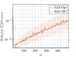
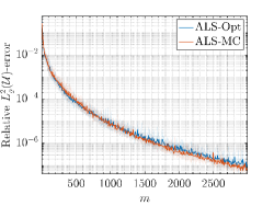
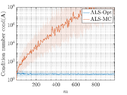
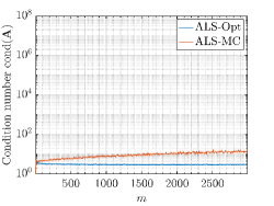
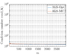
The previous discussion suggests that MC is a bad sampling strategy for polynomial approximation. And indeed, almost all of the above strategies yield significant benefits over MC sampling in low dimensions, where the dimension $d$ may be on the order of five or less. However, such benefits have been consistently observed to lessen as the dimension increases. When $d$ is on the order of 10 or more, the performance gap between MC sampling and any improved sampling strategy is often strikingly less. This is even the case for the near-optimal sampling strategies, in spite of their theoretical optimality. A typical example of effect is shown in Fig. 1, with further examples presented in §LABEL:s:MC-bad. Here LS with MC sampling is unstable and potentially divergent in low dimensions as the number of samples $m$ increases, but in higher dimensions its performance is essentially the same as that LS with a theoretically near-optimal sampling strategy.

$d=1$	$d=4$	$d=32$

Figure 1: In low dimensions, MC sampling from the uniform measure on $\mathcal{U}=[-1,1]^{d}$ is a poor choice. However, it becomes far better as the dimension increases. This figure plots the error (top row) and ($2$-norm) condition number of the LS matrix (bottom row) versus $m$ for (adaptive) LS polynomial approximation using MC samples (ALS-MC) and a near-optimal sampling strategy (ALS-Opt) described in §1.2. The function considered is a quantity of interest of a parametric DE with lognormal diffusion term (see §LABEL:ss:lognormal-pDE). The scaling $m=\max\{n+1,\lceil n\log(n)\rceil\}$ is used in both cases. For MC sampling, the LS problem is highly ill-conditioned when $d=1$, since $m$ scales log-linearly with $n$ rather than log-quadratically, as in (2). This causes a dramatic loss of accuracy due to round-off error. However, as $d$ increases, this LS problem becomes much better conditioned, with both its condition number and the error closely tracking those of the near-optimal strategy.

The aim of this paper is to shed light on this phenomenon. We first document it through a series of numerical experiments on different smooth test functions in both low and high dimensions (in the range $d=1$ to $d=32$). Then we provide a theoretical explanation for why it occurs. We summarize these theoretical results next.

1.4 Nontechnical summary of main theoretical results

Our theoretical analysis centres on polynomial approximation of holomorphic functions of infinitely-many variables. Specifically, we combine the theory of best $n$-term polynomial approximation of such functions with the theories of LS and CS.

1.4.1 Polynomial approximation theory in infinite dimensions

The topic of polynomial approximation theory for infinite-dimensional functions has developed over the last decade or so, motivated by applications in parametric DEs and UQ. See [cohen2015approximation] and [adcock2022sparse, Chpts. 3 & 4] for reviews. A key result in this area is the assertion of certain algebraic rates of convergence for best $n$-term polynomial approximations to certain classes of holomorphic, infinite-dimensional functions.

Consider the infinite hypercube $\mathcal{U}=[-1,1]^{\mathbb{N}}$ equipped with the uniform measure $\varrho$ and let $L^{2}_{\varrho}(\mathcal{U})$ be the Lebesgue space of (complex-valued) square-integrable functions $[-1,1]^{\mathbb{N}}\rightarrow\mathbb{C}$. (For the reader who is unfamiliar with concepts of infinite-dimensional measures and function spaces, we refer to §LABEL:s:polyapp-inf-dim). Any function $f\in L^{2}_{\varrho}(\mathcal{U})$ has an infinite expansion with respect to multivariate orthogonal polynomials, which in this case are tensor products of the univariate Legendre polynomials. The best $n$-term approximation to $f$ is the polynomial formed simply by picking the largest $n$ terms of this expansion in absolute value. In this paper, we denote this approximation as $f_{n}$.

Now let $0<p<1$, $\varepsilon>0$ and $\bm{b}\in\ell^{p}(\mathbb{N})$. Then a key result in this area is that there is a class $\mathcal{H}(\bm{b},\varepsilon)\subset L^{2}_{\varrho}(\mathcal{U})$ of holomorphic functions within which the best $n$-term approximation converges algebraically with rate depending on $1/p$. Specifically,

(4) $${\|f-f_{n}\|}_{L^{2}_{\varrho}(\mathcal{U})}\leq C(\bm{b},\varepsilon,p)\cdot n^{\frac{1}{2}-\frac{1}{p}},\quad\forall f\in\mathcal{H}(\bm{b},\varepsilon),\ n\in\mathbb{N}.$$

In other words, there are classes of functions whose approximation is free from the curse of dimensionality: despite depending on infinitely many variables, they can be approximated with algebraic rate by a finite ($n$-term) polynomial approximation.

The class $\mathcal{H}(\bm{b},\varepsilon)$, which is known as the class of (unit-norm) $(\bm{b},\varepsilon)$-holomorphic functions [chkifa2015breaking, schwab2019deep], is both theoretically interesting, since it defines a class where algebraic rates are obtained, and practically relevant. It was first introduced to describe the parametric regularity of the solutions of certain parametric DEs. It is now known that several important families of parametric DEs have parametric solution maps that belong to such classes (for suitable $\bm{b}$, $\varepsilon$ depending on the DE). These include parametric diffusion equations, parametric heat equations, PDEs over parametrized domains, and parametric initial value problems with affine parametric dependence. See §LABEL:s:pDE-background for some further discussion.

Note that $(\bm{b},\varepsilon)$-holomorphic functions are anisotropic. As we see in §LABEL:s:polyapp-inf-dim, the $j$th component $b_{j}$ of the sequence $\bm{b}$ effectively controls the degree of smoothness of functions in $\mathcal{H}(\bm{b},\varepsilon)$ with respect to the $j$th variable $y_{j}$.

1.4.2 First contribution: sharpness of the rate (4)

In our first contribution, Theorem LABEL:t:alg-rate-sharp, we show that the rate (4) is effectively sharp. In particular, there exist sequences $\bm{b}\in\ell^{p}(\mathbb{N})$ and infinitely many functions $f\in\mathcal{H}(\bm{b},\varepsilon)$ for which $n^{1/2-1/p}$ is the best possible algebraic rate of convergence.

1.4.3 Second contribution: near-optimal approximation in the case of known anisotropy

Our other two theoretical results concern constructing polynomial approximations to functions in $\mathcal{H}(\bm{b},\varepsilon)$ from MC samples, i.e., $\bm{y}_{1},\ldots,\bm{y}_{m}\sim_{\mathrm{i.i.d.}}\varrho$, that attain this algebraic rate. In view of (2), one would generally expect to be able to recover an $n$-term polynomial approximation from $m$ samples via LS for $n$ at most $\sqrt{2m/(c\log m)}$. Combining this upper bound on $n$ with (4), it is therefore tempting to believe that the best one could hope to achieve is

$${\|f-\hat{f}\|}_{L^{2}_{\varrho}(\mathcal{U})}\leq C\cdot\left(m/\log(m)\right)^{\frac{1}{2}(\frac{1}{2}-\frac{1}{p})},$$

when $\bm{b}\in\ell^{p}(\mathbb{N})$. In other words, the algebraic rate is halved, due to the log-quadratic sample complexity (2). However, this is not the case. In Theorem LABEL:t:main-res we show that there is a LS approximation for which the error behaves like

(5) $${\|f-\hat{f}\|}_{L^{2}_{\varrho}(\mathcal{U})}\leq C\cdot\left(m/\log(m)\right)^{\frac{1}{2}-\frac{1}{p}}.$$

Hence the approximation converges with the same rate as that of the best $n$-term approximation, up to constants and the log term. We conclude that MC sampling is not only a good sampling strategy in infinitely many dimensions, but in view of the result in §1.4.2, it is in fact near optimal for the class $\mathcal{H}(\bm{b},\varepsilon)$.

1.4.4 Second contribution: near-optimal approximation in the case of unknown anisotropy

A limitation of any LS scheme is that it requires knowledge of a space in which the function is well approximated. The above result is no different, since it involves a judicious choice of polynomial subspace of dimension $\leq n$ (depending on the parameters $\bm{b}$ and $\varepsilon$) in which one simultaneously obtains the same algebraic rate of convergence (4) as the best $n$-term approximation, while also not suffering from poor sample worst-case complexity bound (3) for MC sampling. At the very least, constructing such a subspace requires a priori knowledge of the parameters $\bm{b}$ and $\varepsilon$. Unfortunately, these are generally unknown in practice.

Because of this limitation, LS is often used as part of an adaptive approximation scheme [migliorati2019adaptive]. Here, rather than a single approximation, one computes a sequence of approximations $\hat{f}^{(1)},\hat{f}^{(2)},\ldots$ and (nested) polynomial subspaces $\mathcal{P}^{(1)}\subseteq\mathcal{P}^{(2)}\subseteq\cdots$, in which the approximation $\hat{f}^{(l)}$ is used to construct the next subspace $\mathcal{P}^{(l+1)}$, typically in a greedy manner. As we see later in this paper, so-called Adaptive Least-Squares (ALS) approximation is often quite effective. However, it lacks theoretical guarantees. It is currently unknown whether such an approximation achieves the algebraic rates of convergence (4) of the best $n$-term approximation (up to constants and log factors).

With this in mind, in the final part of this paper we demonstrate that this issue can be avoided by changing the approximation procedure. By using ideas from CS, we show it is possible to compute a polynomial approximation from $m$ MC samples for which the error behaves like

(6) $${\|f-\hat{f}\|}_{L^{2}_{\varrho}(\mathcal{U})}\leq C\cdot\left(m/\log^{4}(m)\right)^{\frac{1}{2}-\frac{1}{p}},$$

subject to the slightly stricter requirement $\bm{b}\in\ell^{p}_{\mathsf{M}}(\mathbb{N})$, where $\ell^{p}_{\mathsf{M}}(\mathbb{N})$ is the monotone $\ell^{p}$-space. See Theorem LABEL:t:main-res-2. Thus, for a slightly restricted class of functions, it is possible to achieve the same algebraic rates of convergence as the best $n$-approximation in terms of the number of samples $m$, up to a polylogarithmic factor.

This scheme is also practical. We present a series of numerical experiments comparing it to ALS. These show that the CS scheme offers consistently as good as, or sometimes better, performance, while also having theoretical guarantees.

1.4.5 The gap between theory and practice

Our theoretical analysis asserts that MC sampling is near-optimal for polynomial approximation in infinite dimensions. Throughout this article we present numerical experiments for functions of finitely many variables only. Our analysis does apply in finite dimensions – since a function of $d$ variables can be viewed as a function of infinitely many variables that is constant with respect to all but the first $d$ variables – but, as we discuss later, it may not accurately predict the convergence rate when the dimension is small. There is consequently a gap between the theoretical analysis and practice, which leads one naturally to wonder ‘how high is high-dimensional’? In our experiments, we consistently witness this effect in finite dimensions. Most often, it occurs when $d$ is still relatively small (e.g., $d\leq 8$), and certainly by $d=32$, which is the largest dimension considered in this paper. However, we currently have no theoretical understanding of how large $d$ should be for such behaviour to kick in. This is an interesting problem that we leave for future work.

1.4.6 Why bother?

As noted, the development of improved sampling strategies for high-dimensional approximation has been an active area of interest over the last few years. The purpose of this work is to show that MC sampling is actually eminently suitable (in fact, near-optimal) for certain high-dimensional approximation tasks – in particular, those arising from parametric DE problems, which served as the original motivation for much of this line of research.

However, the reader may justifiably be wondering why we bother. Why use MC sampling when we know how to design sampling strategies that are near-optimal regardless of the dimension? For this, we offer several arguments. First, it is both academically interesting and practically relevant to understand the limits of what one stands to gain by changing the sampling strategy. Our results suggest that these gains are limited to lower-dimensional problems, at least for smooth function approximation on bounded domains. Second, methods based on MC sampling have the distinct advantage of allowing one to decouple the function evaluation and function approximation phases. Thus, in the parametric DE context, the major computational burden of evaluating the target function at the sample points can be trivially parallelized. On the other hand, when adaptive approximation schemes (e.g., the aforementioned ALS method) are combined with near-optimal sampling, the sampling strategy also becomes adaptive. Hence, the tasks of sampling the function (i.e., numerically solving a DE) and constructing the polynomial approximation cannot be decoupled. In practice, this might require the design of ad hoc software interfaces or data transfer strategies. Third and finally, MC samples are exchangeable and usually easy to generate. They are found ubiquitously in UQ and machine learning applications; in particular, applications involving legacy data, where one is not afforded the luxury to adapt the samples to the target function and/or approximation scheme.

In summary, there are ample reasons why MC samples may be preferred in practice. Hence investigations into their theoretical and practical performance in high dimensions are particularly relevant.

1.5 Historical context and discussion

Our primary interest is the polynomial approximation of smooth high- and infinite-dimensional functions, with specific focus on Least Squares (LS) and Compressed Sensing (CS) techniques. LS approximation is a classical topic, with a genesis that can be traced back to very early work by Gauss and Legendre at the turn of the 18th and 19th centuries [stigler1981gauss]. LS is utilized in countless areas of applied mathematics and statistics, with eminent examples such as function approximation (of direct interest in this paper) and statistical regression.

Our work stems from a vigorous research stream started in the early 2010s, characterized by renewed interest towards LS [cohen2013stability, chkifa2015discrete, migliorati2014analysis] and the application of the CS paradigm [doostan2011nonadapted, mathelin2012compressed, rauhut2012sparse] in the context of high-dimensional function approximation. The fast development of this research area is in tandem with progress in the fields of stochastic and parametric DEs. For stochastic DEs, this is strongly related to polynomial chaos technique. This dates back to the 1930s [wiener1938homogeneous], and has found tremendous success in computational science and engineering since its inception in the 1990s [ghanem1990polynomial] and thanks to a series of influential works in the 2000s, such as [xiu2002wiener, babuska2008stochastic], which contributed to the development of the UQ field (see also [smith2013uncertainty, sullivan2015introduction]). As noted, a signature result for parametric DEs was the discovery that solution maps of a large class of parametric models admit best $n$-term polynomial approximation rates that are independent of the number of parameters, and therefore free from the curse of dimensionality. For more details about parametric DEs and historical remarks we refer to [cohen2015approximation] and [adcock2022sparse, Chpt. 4].

Although considerably younger than LS, MC sampling is also a classical technique. The happenings that led to its widespread use in computational science are intertwined with the construction of the first electronic programmable digital computer (ENIAC), pioneering simulations of complex physical systems, and – regrettably – the creation of the first nuclear weapons in the 1940s. The history of the MC method features scientists of the calibre of Fermi, von Neumann, Ulam and Metropolis [metropolis1990alamos, metropolis1987beginning].

One of the most popular applications of MC sampling is numerical quadrature. It is well known that the MC quadrature error scales proportionally to $m^{-1/2}$, where $m$ is the number of MC samples of the function to be integrated (see, e.g., [owen2013monte, Section 2.1]). Remarkably, this decay rate is independent of the number of function’s variables, which – at least, intuitively – motivates the use of MC in high dimensions. We recall, though, that in this work we are concerned with high-dimensional function approximation, as opposed to quadrature. In particular, it is worth noting that best $n$-term approximation error rates of the smooth high-dimensional functions of interest in this paper decay much faster than the MC quadrature error (see §1.4.1).

Naturally, any discussion of LS and MC sampling would be incomplete without a word on regression. We now warn the reader that this is not a paper on statistical regression. Statistical regression refers to the problem of fitting a model to noisy data under some probabilistic assumptions on the noise (e.g., homoscedasticity). This is not the perspective adopted in this paper. In fact, our goal is the accurate and stable approximation of a ‘ground truth’ function from pointwise samples, where the noise corrupting the samples need not be modelled as a random variable. For a more in-depth discussion of the differences between the function approximation and statistical regression settings, we refer to [guo2020constructing, §1.1], of which we share the same viewpoint.

1.6 Outline

In §2 we present an overview of polynomial approximation of multivariate functions and (weighted) LS. In §3 we present relevant theory for (weighted) LS, before discussing MC sampling and the near-optimal strategy mentioned in §1.2. In §LABEL:s:MC-bad we present numerical experiments demonstrating the main phenomenon considered in this work. We then turn our attention to its theoretical explanation. In §LABEL:s:polyapp-inf-dim we introduce and review polynomial approximation theory for $(\bm{b},\varepsilon)$-holomorphic functions. We present our first result in §LABEL:s:main-res, i.e., the existence of a LS approximation achieving the bound (5). Finally, we consider CS schemes in §LABEL:s:polyappCS, including both the error bound (6) and a numerical comparison between ALS and CS.

This paper also has supplementary materials. These contain background on infinite-dimensional measures (§LABEL:s:inf_dim_measures), proofs of various results (§LABEL:s:proofs), additional information on the experimental setup (§LABEL:s:additional-info), background on parametric DEs (§LABEL:s:pDE-background) and further experiments (§LABEL:s:further-experiments). MATLAB code reproducing all the experiments is available at https://github.com/benadcock/is-MC-bad.

2 Polynomials and least-squares polynomial approximation

In this section, we describe multivariate orthogonal polynomials and polynomial approximation via LS. In order to keep the technical level reasonable, we consider the finite-dimensional case only. The infinite-dimensional case is introduced in §LABEL:s:polyapp-inf-dim.

2.1 Univariate notation

Let $\varrho$ be a probability measure on $[-1,1]$ and write $L^{2}_{\varrho}([-1,1])$ for the corresponding Lebesgue space of square-integrable functions $f:[-1,1]\rightarrow\mathbb{C}$. We assume that $\varrho$ generates a unique sequence of orthonormal polynomials $\{\psi_{\nu}\}_{\nu\in\mathbb{N}_{0}}\subset L^{2}_{\varrho}([-1,1])$. In other words,

$$\langle\psi_{\nu},\psi_{\nu^{\prime}}\rangle=\delta_{\nu,\nu^{\prime}},\quad\forall\nu,\nu^{\prime}\in\mathbb{N}_{0},\quad\text{and}\quad\mathrm{span}\{\psi_{0},\ldots,\psi_{n}\}=\mathbb{P}_{n},\quad\forall n\in\mathbb{N}_{0},$$

where $\mathbb{P}_{n}$ is the space of polynomials of degree at most $n$. Note that this is a mild assumption (see, e.g., [narayan2018computation, §2.1]). Two particular cases we focus on in this paper are the uniform and Chebyshev (arcsine) measures

$$\,\mathrm{d}\varrho(y)=2^{-1}\,\mathrm{d}y,\qquad\,\mathrm{d}\varrho(y)=(\pi\sqrt{1-y^{2}})^{-1}\,\mathrm{d}y,$$

which generate the Legendre and (first kind) Chebyshev polynomials, respectively.

2.2 Multivariate polynomial approximation

Let $d\in\mathbb{N}$ and consider the symmetric hypercube $\mathcal{U}=[-1,1]^{d}$. We define a probability measure over $\mathcal{U}$ via tensor products. Abusing notation, we write $\varrho=\varrho\times\cdots\times\varrho$ for this measure, where on the right-hand side $\varrho$ denotes the probability measure on $[-1,1]$.

Let $L^{2}_{\varrho}(\mathcal{U})$ be the Lebesgue space of square-integrable functions $f:\mathcal{U}\rightarrow\mathbb{C}$. We construct an orthonormal polynomial basis for this space via tensor products. Writing $\bm{\nu}=(\nu_{1},\ldots,\nu_{d})\in\mathbb{N}^{d}_{0}$ for an arbitrary multi-index, we define

$$\Psi_{\bm{\nu}}(\bm{y})=\psi_{\nu_{1}}(y_{1})\cdots\psi_{\nu_{d}}(y_{d}),\qquad\bm{y}=(y_{i})^{d}_{i=1}\in\mathcal{U}.$$

The set $\{\Psi_{\bm{\nu}}\}_{\bm{\nu}\in\mathbb{N}^{d}_{0}}\subset L^{2}_{\varrho}(\mathcal{U})$ forms an orthonormal basis. Hence any function $f\in L^{2}_{\varrho}(\mathcal{U})$ has the convergent expansion

(7) $$f=\sum_{\bm{\nu}\in\mathbb{N}^{d}_{0}}c_{\bm{\nu}}\Psi_{\bm{\nu}},\qquad\text{where }c_{\bm{\nu}}=\langle f,\Psi_{\bm{\nu}}\rangle_{L^{2}_{\varrho}(\mathcal{U})}=\int_{\mathcal{U}}f(\bm{y})\overline{\Psi_{\bm{\nu}}(\bm{y})}\,\mathrm{d}\varrho(\bm{y}).$$

We are interested in $n$-term approximations to such functions. An $n$-term approximation to $f$ based on an multi-index set $S\subset\mathbb{N}^{d}_{0}$, $|S|=n$, has the form

(8) $$f_{S}=\sum_{\bm{\nu}\in S}c_{\bm{\nu}}\Psi_{\bm{\nu}}.$$

Due to Parseval’s identity, the error of such an approximation is determined by the size of the coefficients $c_{\bm{\nu}}$ not included in $S$. Specifically,

(9) $${\|f-f_{S}\|}^{2}_{L^{2}_{\varrho}(\mathcal{U})}=\sum_{\bm{\nu}\notin S}|c_{\bm{\nu}}|^{2}.$$

2.3 Choosing $S$

In standard multivariate polynomial approximation it is common to make an a priori choice of $S$ with some prescribed structure (see, e.g., [guo2020constructing]). Given $\ell\in\mathbb{N}_{0}$, classical examples are the tensor-product index set of order $\ell$,

$$S^{\mathsf{TP}}_{\ell}=\left\{\bm{\nu}=(\nu_{k})_{k=1}^{d}\in\mathbb{N}_{0}^{d}:\max\{\nu_{1},\ldots,\nu_{d}\}\leq\ell\right\},$$

or the total degree index set of order $\ell$,

$$S^{\mathsf{TD}}_{\ell}=\left\{\bm{\nu}=(\nu_{k})_{k=1}^{d}\in\mathbb{N}_{0}^{d}:\nu_{1}+\cdots+\nu_{d}\leq\ell\right\}.$$

However, the cardinality of these index sets scales exponentially with the dimension $d$, making them poorly suited in all but low-dimensional problems. Specifically, $|S^{\mathsf{TP}}_{\ell}|=(\ell+1)^{d}$ and $|S^{\mathsf{TD}}_{\ell}|={\ell+d\choose d}$ for any $\ell\in\mathbb{N}_{0}$ and $d\in\mathbb{N}$. Applying Stirling’s formula, one deduces that $|S^{\mathsf{TD}}_{\ell}|\sim\ell^{d}/d!$ as $\ell\to\infty$ for fixed $d$. This effect can be partially mitigated by working with hyperbolic cross index sets (see, e.g., [guo2020constructing]). Yet, the cardinalities of these sets also grow exponentially with dimension.

Alternatively, one can look to replace such isotropic sets with anisotropic variants. High-dimensional functions may be highly anisotropic, i.e., they may depend more strongly on some variables than others. The aforementioned index sets fail to capture this behaviour, thus potentially leading to poor approximations. However, selecting a good anisotropic set a priori requires detailed knowledge about the function $f$, which is typically unavailable in practice.

A theoretical alternative is provided by the concept of best $n$-term approximation. Here, one does away with the classical notion of polynomial degree (as described by the parameter $\ell$ in $S^{\mathsf{TP}}_{\ell}$ and $S^{\mathsf{TD}}_{\ell}$) and instead seeks an optimal index set in a function-dependent manner by minimizing the error (9) over all possible sets. A best $n$-term approximation $f_{n}$ of $f$ is thus defined as

(10) $$f_{n}=f_{S^{*}},\qquad\text{where }S^{*}\in{\underset{}{\operatorname{argmin}}}\{{\|f-f_{S}\|}_{L^{2}_{\varrho}(\mathcal{U})}:S\subset\mathbb{N}^{d}_{0},\ |S|=n\}.$$

It follows straightforwardly from (9) that $S^{*}$ consists of those multi-indices corresponding to the $n$ largest coefficients $c_{\bm{\nu}}$ of $f$ in absolute value; that is to say, $S^{*}=\{\bm{\nu}_{1},\bm{\nu}_{2},\ldots,\bm{\nu}_{n}\}$, where $\bm{\nu}_{1},\bm{\nu}_{2},\ldots$ are such that $|c_{\bm{\nu}_{1}}|\geq|c_{\bm{\nu}_{2}}|\geq\cdots$.

Unfortunately, the best $n$-term approximation is a theoretical benchmark. It is generally impossible to construct, since doing so would generically involve computing and sorting infinitely-many coefficients – something that clearly cannot be done from the finite data (1). A more practical approach is therefore to construct a set $S$ – or more precisely, a nested sequence of set $S^{(1)}\subseteq S^{(2)}\subseteq\cdots$ – in a function dependent, adaptive manner. This is typically done via a greedy procedure, with multi-indices being added according to some importance criterion. The aforementioned ALS method is a procedure of this type. We discuss it further in §LABEL:s:ALS and §LABEL:ss:adaptive-LS.

Regardless of how the index set (or sets) is constructed, however, it is generally useful to restrict one’s attention sets with certain structure. A lower set (also known as monotone or downward closed – see, e.g., [cohen2015approximation]) is a set $S\subseteq\mathbb{N}^{d}_{0}$ for which

$$(\bm{\nu}\in S\text{ and }\bm{\mu}\leq\bm{\nu})\ \Rightarrow\ \bm{\mu}\in S,$$

(here the inequality $\bm{\mu}\leq\bm{\nu}$ is understood componentwise). Lower sets are ubiquitous in multivariate polynomial approximation, with (isotropic or anisotropic) tensor-product, total degree and hyperbolic cross index sets all being examples. Lower sets are also commonly employed in adaptive strategies such as ALS (see §LABEL:ss:adaptive-LS), so as to make the greedy selection procedure tractable. Indeed, given a lower set $S^{(l)}$ there are only finitely many multi-indices $\bm{\nu}\in\mathbb{N}^{d}_{0}\backslash S^{(l)}$ for which $S^{(l)}\cup\{\bm{\nu}\}$ is also lower.

2.4 Weighted least-squares polynomial approximation

Fix a set multi-indices $S\subset\mathbb{N}^{d}_{0}$, $|S|=n$, and consider $m\geq n$ noisy samples (1) of a function $f\in L^{2}_{\varrho}(\mathcal{U})$ at sample points $\bm{y}_{1},\ldots,\bm{y}_{m}\in\mathcal{U}$. We wish to compute an approximation to $f$ from the polynomial space defined by $S$: namely, the subspace

$$\mathcal{P}_{S}=\mathrm{span}\{\Psi_{\bm{\nu}}:\bm{\nu}\in S\}\subset L^{2}_{\varrho}(\mathcal{U}).$$

Given a positive and almost everywhere finite weight function $w:\mathcal{U}\rightarrow\mathbb{R}$, we define a weighted least-squares approximation to $f$ as

(11) $$\hat{f}\in{\underset{p\in\mathcal{P}_{S}}{\operatorname{argmin}}}{\frac{1}{m}}\sum^{m}_{i=1}w(\bm{y}_{i})|f(\bm{y}_{i})+e_{i}-p(\bm{y}_{i})|^{2}.$$

This is readily computed by solving an algebraic LS problem for the coefficients of $\hat{f}$. Indeed, let $\bm{\nu}_{1},\ldots,\bm{\nu}_{n}$ be an enumeration of the indices in $S$. Then

$$\hat{f}=\sum^{n}_{i=1}\hat{c}_{i}\Psi_{\bm{\nu}_{i}},\quad\text{where }\hat{\bm{c}}=(\hat{c}_{i})^{n}_{i=1}\in{\underset{\bm{z}\in\mathbb{C}^{n}}{\operatorname{argmin}}}{\left\|\bm{A}\bm{z}-\bm{f}\right\|}_{2}^{2},$$

and the LS matrix $\bm{A}\in\mathbb{C}^{m\times n}$ and vector $\bm{f}\in\mathbb{C}^{m}$ are given by

(12) $$\bm{A}=\left(\sqrt{w(\bm{y}_{i})/m}\Psi_{\bm{\nu}_{j}}(\bm{y}_{i})\right)^{m,n}_{i,j=1},\qquad\bm{f}=\left(\sqrt{w(\bm{y}_{i})/m}(f(\bm{y}_{i})+e_{i})\right)^{m}_{i=1}.$$

3 Theory of (weighted) least-squares approximation

In this section, we present some elementary theory for weighted LS approximation. For the sake of generality, in the majority of this section we consider an arbitrary $n$-dimensional subspace $\mathcal{P}\subset L^{2}_{\varrho}(\mathcal{U})$ (i.e., not necessarily a polynomial subspace of the form $\mathcal{P}=\mathcal{P}_{S}$). We write $\{\Psi_{i}\}^{n}_{i=1}$ for an orthonormal basis for $\mathcal{P}$. However, for convenience, we make the mild assumption that the constant function $p(\bm{y})=1$, $\forall\bm{y}\in\mathcal{U}$, is an element of $\mathcal{P}$. Note that this always holds when $\mathcal{P}=\mathcal{P}_{S}$ and $S$ is a lower set.

3.1 Accuracy and stability

Given sample points $\bm{y}_{1},\ldots,\bm{y}_{m}\in\mathcal{U}$ and a weight function $w:\mathcal{U}\rightarrow\mathbb{R}$, define the discrete semi-norm

$${\|f\|}^{2}_{\mathsf{disc},w}=\frac{1}{m}\sum^{m}_{i=1}w(\bm{y}_{i})|f(\bm{y}_{i})|^{2},\quad\forall f\in L^{2}_{\varrho}(\mathcal{U})\cap C(\mathcal{U}),$$

(here $C(\mathcal{U})$ is the set of continuous functions on $\mathcal{U}$) and the discrete stability constants

$$\alpha_{w} =\inf\left\{{\|p\|}_{\mathsf{disc},w}:p\in\mathcal{P},\ {\left\|p\right\|}_{L^{2}_{\varrho}(\mathcal{U})}=1\right\},$$

$$\beta_{w} =\sup\left\{{\|p\|}_{\mathsf{disc},w}:p\in\mathcal{P},\ {\left\|p\right\|}_{L^{2}_{\varrho}(\mathcal{U})}=1\right\},$$

Notice that $\alpha_{w}=\sigma_{\min}(\bm{A})$ and $\beta_{w}=\sigma_{\max}(\bm{A})$, where is the LS matrix (12).

Lemma 3.1 (Accuracy and stability of weighted LS).

Let $\mathcal{P}\subset L^{2}_{\varrho}(\mathcal{U})\cap C(\mathcal{U})$ with $1\in\mathcal{P}$, $f\in L^{2}_{\varrho}(\mathcal{U})\cap C(\mathcal{U})$, $\bm{e}\in\mathbb{C}^{m}$, $\bm{y}_{1},\ldots,\bm{y}_{m}\in\mathcal{U}$ and $w:\mathcal{U}\rightarrow\mathbb{R}$ be such that $w(\bm{y}_{i})>0$, $\forall i\in[m]:=\{1,\ldots,m\}$. If $\alpha_{w}>0$ then the problem

(13) $$\min_{p\in\mathcal{P}}{\frac{1}{m}}\sum^{m}_{i=1}w(\bm{y}_{i})|f(\bm{y}_{i})+e_{i}-p(\bm{y}_{i})|^{2}$$

has a unique solution $\hat{f}$. This solution satisfies

(14) $${\|f-\hat{f}\|}_{L^{2}_{\varrho}(\mathcal{U})}\leq\inf_{p\in\mathcal{P}}\left\{{\|f-p\|}_{L^{2}_{\varrho}(\mathcal{U})}+\frac{1}{\alpha_{w}}{\|f-p\|}_{\mathsf{disc},w}\right\}+\frac{\beta_{w}}{\alpha_{w}}{\left\|\bm{e}\right\|}_{\infty}.$$

Also, the ($2$-norm) condition number of the LS matrix satisfies $\mathrm{cond}(\bm{A})=\beta_{w}/\alpha_{w}$.

This result is standard (see, e.g., [migliorati2014analysis, Prop. 1]). We include a short proof in §LABEL:s:proofs for completeness. Note that the last statement is immediate, since $\mathrm{cond}(\bm{A})=\sigma_{\max}(\bm{A})/\sigma_{\min}(\bm{A})$ by definition. The main takeaway from this lemma is that the accuracy and stability of $\hat{f}$ are determined by the size of the constants $\alpha_{w}$ and $\beta_{w}$. In the next subsection, we discuss how to control these constants in the case of random sampling. In doing so, we also obtain an estimate for the sample complexity.

3.2 Sample complexity

We now consider the sample complexity of weighted LS approximation in the case of random sampling. Specifically, we now assume that $\bm{y}_{1},\ldots,\bm{y}_{m}\sim_{\mathrm{i.i.d.}}\mu$, where $\mu$ is some probability measure with support in $\mathcal{U}$.

The analysis of this type of sampling strategy involves the (reciprocal) Christoffel function of the subspace $\mathcal{P}$ [cohen2013stability]:

$$\mathcal{K}(\mathcal{P})(\bm{y})=\sup\left\{|p(\bm{y})|^{2}:p\in\mathcal{P},\ {\left\|p\right\|}_{L^{2}_{\varrho}(\mathcal{U})}=1\right\},\quad\forall\bm{y}\in\mathcal{U}.$$

Observe that $\mathcal{K}(\mathcal{P})(\bm{y})\geq 1$, $\forall\bm{y}\in\mathcal{U}$, since, by assumption, the function $1\in\mathcal{P}$. It is also a short argument to show that $\mathcal{K}(\mathcal{P})$ has the equivalent expression

(15) $$\mathcal{K}(\mathcal{P})(\bm{y})=\sum^{n}_{i=1}|\Psi_{i}(\bm{y})|^{2},\quad\forall\bm{y}\in\mathcal{U},$$

where $\{\Psi_{i}\}^{n}_{i=1}$ is any orthonormal basis for $\mathcal{P}$. Given $\mathcal{K}$ and a weight function $w:\mathcal{U}\rightarrow(0,\infty)$, we now also define

(16) $$\kappa(\mathcal{P};w)=\sup_{\bm{y}\in\mathcal{U}}w(\bm{y})\mathcal{K}(\mathcal{P})(\bm{y}).$$

Theorem 1.

[Sample complexity of weighted LS with random sampling] Let $\mathcal{P}\subset L^{2}_{\varrho}(\mathcal{U})\cap C(\mathcal{U})$ with $\dim(\mathcal{P})=n$ and $1\in\mathcal{P}$, $0<\epsilon<1$ and $\mu$ be a probability measure on $\mathcal{U}$ such that

(17) $$\,\mathrm{d}\mu(\bm{y})=(w(\bm{y}))^{-1}\,\mathrm{d}\varrho(\bm{y})$$

for some strictly positive and finite almost everywhere weight function $w:\mathcal{U}\rightarrow\mathbb{R}$. Let $\bm{y}_{1},\ldots,\bm{y}_{m}\sim_{\mathrm{i.i.d.}}\mu$, where $m$ satisfies

(18) $$m\geq 7\cdot\kappa(\mathcal{P};w)\cdot\log(2n/\epsilon).$$

Then the following holds with probability at least $1-\epsilon$. For any $f\in L^{2}_{\varrho}(\mathcal{U})\cap C(\mathcal{U})$, the solution $\hat{f}$ of the weighted LS problem (13) is unique and satisfies

(19) $${\|f-\hat{f}\|}_{L^{2}_{\varrho}(\mathcal{U})}\leq\inf_{p\in\mathcal{P}}\left\{{\|f-p\|}_{L^{2}_{\varrho}(\mathcal{U})}+2{\|f-p\|}_{\mathsf{disc},w}\right\}+2{\|\bm{e}\|}_{\infty}.$$

Moreover, the condition number satisfies $\mathrm{cond}(\bm{A})\leq 2$.

This result is based on standard ideas, in particular, the use of the matrix Chernoff inequality (see, e.g., [cohen2017optimal, Thm. 2.1]). We include a short proof in §LABEL:s:proofs for completeness. Note that the number $7$ in (18) is somewhat arbitrary. As can be seen from the proof, one can replace it with a smaller constant at the expense of larger constants in the error and condition number bounds.

The most important aspect of this result is the sample complexity bound (18). Since $\mu$ is a probability measure, (17) implies that

(20) $$\int_{\mathcal{U}}(w(\bm{y}))^{-1}\,\mathrm{d}\varrho(\bm{y})=1,$$

and orthonormality and the alternative expression (15) for $\mathcal{K}(\mathcal{P})$ imply that

(21) $$\int_{\mathcal{U}}\mathcal{K}(\mathcal{P})(\bm{y})\,\mathrm{d}\varrho(\bm{y})=n$$

and

$$\kappa(\mathcal{P};w)=\int_{\mathcal{U}}\kappa(\mathcal{P};w)/w(\bm{y})\,\mathrm{d}\varrho(\bm{y})\geq\int_{\mathcal{U}}\mathcal{K}(\mathcal{P})(\bm{y})\,\mathrm{d}\varrho(\bm{y})=n.$$

Hence $\kappa(\mathcal{P};w)\geq n$ for any $\mathcal{P}$ and $w$. As a result, the sample complexity bound (18) is always at least log-linear in $n$. In the next subsection, we show that it is generally superlinear in $n$. However, in §LABEL:ss:opt-samp-scheme we show that it is always possible to choose the sampling measure $\mu$ so as to achieve the optimal value of the right-hand side of (18).

3.3 The case of Monte Carlo sampling

MC sampling corresponds to the choice $\mu=\varrho$, in which case (17) holds with $w=1$. The approximation (13) is correspondingly an unweighted LS approximation. In this case, the sample complexity estimate (18) takes the form

(22) $$m\geq c\cdot\kappa(\mathcal{P})\cdot\log(n/\epsilon),\quad\text{where }\kappa(\mathcal{P})=\kappa(\mathcal{P};1)={\left\|\mathcal{K}(\mathcal{P})\right\|}_{L^{\infty}(\mathcal{U})}.$$

Recall that $\kappa(\mathcal{P})\geq n=\dim(\mathcal{P})$. Unfortunately, $\kappa(\mathcal{P})$ can be arbitrarily large, even in cases such as Chebyshev and Legendre polynomial approximation. We now state two standard results, which are based on [chkifa2015discrete, chkifa2014high, chkifa2018polynomial] (see also [adcock2022sparse, Props. 5.13 & 5.17]).