Construction of a traversable wormhole from a suitable embedding function.

Abstract

In this work, we construct a traversable wormhole by providing a suitable embedding function ensuring the fulfilling of the flaring–out condition. The solution contains free parameters that are reduced through the study of the acceptable conditions of a traversable wormhole. We compute both the quantifier of exotic matter and the quasi–normal modes through the $13^{th}$ order WKB as a function of the remaining free parameters. We obtain that the wormhole geometry can be sustained by a finite amount of exotic matter and seems to be stable under scalar perturbations.

I Introduction

Since the seminal work by Morris and Thorne Morris:1988cz , the study of traversable wormholes has remain as an attractive research line for many years given the intriguing features it encodes Morris:1988tu ; Alcubierre:2017pqm ; Visser:1995cc ; Lobo:2005us ; Garattini:2019ivd ; Stuchlik:2021guq ; Bronnikov:2021ods ; Blazquez-Salcedo:2021udn ; Churilova:2021tgn ; Konoplya:2021hsm ; Tello-Ortiz:2021kxg ; Bambi:2021qfo ; Capozziello:2020zbx ; Blazquez-Salcedo:2020czn ; Berry:2020tky ; Maldacena:2020sxe ; Garattini:2020kqb . However, the detection of gravitational waves by LIGO/Virgo from the merger of binary black holes LIGOScientific:2016aoc ; LIGOScientific:2016sjg ; LIGOScientific:2017bnn has driven the attention on the possibility of considering wormholes as black holes mimickers Bueno:2017hyj ; Cardoso:2016oxy ; Konoplya:2016hmd . To be more precise, as the ringdown phase of black hole mergers is dominated by the quasinormal modes of the final object, it has been claimed that wormholes can mimic black holes based on the similitude of their quasinormal modes spectrum.

From a technical point of view, any traversable wormhole could be constructed by providing its geometry in terms of free parameters which should be constrained based on the acceptability conditions it must satisfy: i) the existence of a throat connecting two asymptotically flat regions, ii) small tidal forces bearable by a human being iii) finite proper time to traverse the throat, among others. However, the fulfilling of all the requirements is not always possible. For example, the solution should not be asymptotically flat or should require an infinite amount of exotic matter supporting it. It should be emphasized that the above mentioned requirements are not universal but sufficient for a wormhole to be a physically viable and suitable for interstellar travel by human beings. For example, we can construct asymptotically AdS wormholes which are suitable for interstellar travels. Blazquez-Salcedo:2020nsa . Nevertheless, in this work, it is our main goal to construct an asymptotically flat traversable wormhole supported by a finite amount of exotic matter by assuming a general embedding function. Besides, we explore its stability thorough its response to scalar perturbation.

The response of a wormhole to perturbations is dominated by damped oscillations called quasi–normal modes. The computation of the QNM modes can be performed through a variety of methods (for an incomplete list see Konoplya:2022tvv ; Churilova:2021nnc ; Konoplya:2020jgt ; Konoplya:2020bxa ; Konoplya:2019nzp ; Rincon:2021gwd ; Panotopoulos:2020mii ; Rincon:2020cos ; Rincon:2020iwy ; Rincon:2020pne ; Xiong:2021cth ; Zhang:2021bdr ; Panotopoulos:2019gtn ; Lee:2020iau ; Churilova:2019qph ; Oliveira:2018oha ; Panotopoulos:2017hns and references therein, for example). However, in this work, we shall use the recently developed WKB approximation to the $13^{th}$ order which has brought the attention of the community Konoplya:2019hlu . It should be emphasized that, for the application of the method in the context of traversable wormholes, a bell–shape potential must be ensured. In this work, we study the QNM for the model after providing the suitable sets of parameters that ensure a bell–shaped potential.

This work is organized as follows. In section II we review the mains aspects related to traversable wormholes. Next, in section III we propose the embedding function, obtain the shape of the wormhole and analyse the quantifier of the exotic matter. In section IV we implement the $13^{th}$ order WKB approximation to compute and interpret the quasinormal modes associated to the scalar perturbations of the wormhole. Finally, in the last section we conclude the work.

II Traversable wormholes

Let us consider the spherically symmetric line element

$$ds^{2}=-e^{2\phi}dt^{2}+dr^{2}/(1-b/r)+r^{2}(d\theta^{2}+\sin^{2}\theta d\phi^{2}),$$

with $\phi=\phi(r)$ and $b=b(r)$ the redshift and shape functions respectively. Assuming that (II) is a solution of Einstein’s equations

$$R_{\mu\nu}-\frac{1}{2}g_{\mu\nu}R=\kappa T_{\mu\nu},$$ (2)

with $\kappa=8\pi G/c^{4}$ , sourced by $T^{\mu}_{\nu}=diag(-\rho,p_{r},p_{t},p_{t})$ we arrive at

$$\rho = \frac{1}{8\pi}\frac{b^{\prime}}{r^{2}}$$ (3)

$$p_{r} = -\frac{1}{8\pi}\left[\frac{b}{r^{3}}-2\left(1-\frac{b}{r}\right)\frac{\phi^{\prime}}{r}\right]$$ (4)

$$p_{t} = \frac{1}{8\pi}\left(1-\frac{b}{r}\right)\bigg{[}\phi^{\prime\prime}+(\phi^{\prime})^{2}-\frac{b^{\prime}r-b}{2r^{2}(1-b/r)}\phi^{\prime}$$ (5)

$$-\frac{b^{\prime}r-b}{2r^{3}(1-b/r)}+\frac{\phi^{\prime}}{r}\bigg{]}.$$

In what follows we shall describe the main aspects of a traversable wormhole by its embedding in the three dimensional Euclidean space. First, note that as our solution is spherically symmetric, we can consider $\theta=\pi/2$ without loss of generality. Now, considering a fixed time, $t=constant$, the line element reads

$$ds^{2}=\frac{dr^{2}}{1-b/r}+r^{2}d\phi^{2}.$$ (6)

The surface described by (6) can be embedded in $\mathbf{R}^{3}$ where the metric in cylindrical coordinates $(r,\phi,z)$ reads

$$ds^{2}=dz^{2}+dr^{2}+r^{2}d\phi^{2}.$$ (7)

Next, as $z$ is a function of the radial coordinate we have

$$dz=\frac{dz}{dr}dr,$$ (8)

from where

$$ds^{2}=\left[1+\left(\frac{dz}{dr}\right)^{2}\right]dr^{2}+r^{2}d\phi^{2}.$$ (9)

Finally, from (6) and (9) we obtain

$$\frac{dz}{dr}=\pm\left(\frac{r}{b}-1\right)^{-1/2},$$ (10)

where is clear that $b>0$ for $r\in[r_{0},\infty)$. At this point some comments are in order. First, the wormhole geometry must be endowed with minimum radius which leads to $dz/dr\to\infty$ as $r\to b_{0}$ (that occurs when $b=r$). Accordingly, the existence of a minimum radius requires that at $r=b_{0}$ the shape function must be $b=b_{0}$. Second, we demand that the solution is asymptotically flat which implies both, $b/r\to 0$ (from where $dz/dr\to 0$) and $\phi\to 0$ as $r\to\infty$. Third, as as the conditions

$$\lim\limits_{r\to b_{0}}\frac{dz}{dr}\to\infty$$ (11)

$$\lim\limits_{r\to\infty}\frac{dz}{dr}=0,$$ (12)

must be satisfied, the smoothness of the geometry is ensured whenever the embedding surface flares out at or near the throat, namely

$$\frac{d^{2}r}{dz^{2}}>0,$$ (13)

from where

$$\frac{b-b^{\prime}r}{2b^{2}}>0,$$ (14)

which corresponds to the flaring–out condition.

It is worth mentioning that, the flaring out condition (14) leads to the violation of the null energy condition (NEC) as we shall see in what follows. Let us define the quantity

$$\xi=-\frac{p_{r}+\rho}{|\rho|}=\frac{b/r-b^{\prime}-2(r-b)\phi^{\prime}}{|b^{\prime}|},$$ (15)

which can be written as

$$\xi=\frac{2b^{2}}{r|b^{\prime}|}\frac{d^{2}r}{dz^{2}}-2(r-b)\frac{\phi^{\prime}}{|b^{\prime}|}$$ (16)

Now, as $(r-b)\to 0$ at the throat, we have

$$\xi=\frac{2b^{2}}{r|b^{\prime}|}\frac{d^{2}r}{dz^{2}}>0$$ (17)

so that

$$\xi=-\frac{p_{r}+\rho}{|\rho|}>0.$$ (18)

Note that if $\rho>0$ the above condition implies $p_{r}<0$ which entails that $T^{1}_{1}$ should be interpreted as a tension. Furthermore, if we define $\tau=-p_{r}$ the flaring out condition leads to

$$\tau-\rho>0,$$ (19)

which implies that, for this exotic matter, the throat tension must be greater than the total energy density which violates the NEC, as we stated before. Although there is not evidence of exotic matter in the universe, we can minimize the amount required to construct a traversable wormhole by demanding that the quantifier Visser:2003yf

$$I=\int dV(\rho+p_{r})=-\int\limits_{r_{0}}^{\infty}(1-b^{\prime})\left[\ln\left(\frac{e^{2\phi}}{1-b/r}\right)\right]dr$$

is finite.

From a technical point of view, the construction of traversable wormholes require solving the system (3)-(5), namely three equations with five unknowns. The strategy should be either supplying the metric functions that satisfy the geometric constraints listed above or giving one of the metrics and an auxiliary condition, namely an equation of state or a metric constraint. In this work we follow an alternative route which consists of proposing a suitable embedding function.

III A wormhole model

In this section, we construct a traversable wormhole geometry by providing a general embedding function with the aim to integrate Eq. (10) and obtain the shape function $b$. Note that, although Eq. (10) can always be inverted numerically, in this work we look for analytical solutions so we propose

$$z(r)=\sqrt{\log\left(a+\left(\frac{cr}{r_{0}}+d\right)^{2}\right)}$$ (21)

where $a$, $c$ and $d$ are free parameters. The free parameters can be constrained by imposing both the existence of a throat (a minimum radius $r_{0}$) and the flaring out condition given by Eqs. (11) and (12) which lead to

$$a=1-c^{2}-2cd-d^{2}$$ (22)

In figure 1 we show the embedding function for different values of the parameters involved. Note that the profiles flare out slowly as both $c$ and $d$ increases.

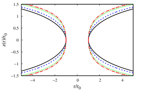
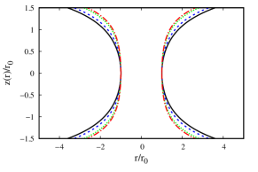
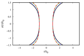
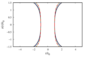
Figure 1: Embedding diagrams for $c=0.4$ (first row, left panel), $0.8$ (first row, right panel), $1.2$ (second row, first panel), $1.6$ (second row, right panel) and $d=0.2$ (black), $d=0.6$ (blue), $d=1.4$ (green), $d=1.8$ (red)

The shape function is obtained by replacing (21) in (10). As a result we obtain

$$b(r)=\frac{c^{2}\zeta^{2}r}{c^{2}\zeta^{2}+r_{0}^{2}\left(a+\zeta^{2}\right)^{2}\log\left(a+\zeta^{2}\right)}$$ (23)

where

$$\zeta=\left(\frac{cr}{r_{0}}+d\right).$$ (24)

Note that the conditions $z(r_{0})=0$ and $b(r_{0})=r_{0}$ hold, as expected. In figure 2 we show the embedding function and the shape function for different values of the parameters involved. Note that, the solution is asymptotically flat as required.

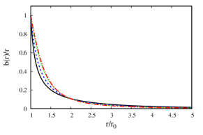
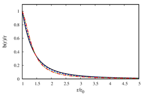
Figure 2: Plots of $b/r$ as a function of $r/r_{0}$ for $c=0.4$ (first row, left panel), $0.8$ (first row, right panel), $1.2$ (second row, left panel), $1.6$ (second row, right panel) and d = 0.2 (black), $d=0.6$ (blue), $d=1.4$ (green), $d=1.8$ (red)

In order to specify the wormhole metric completely, we must propose a suitable redshift function. In this work we shall take the simplest choice, namely $\phi=0$, so the solution has a vanishing radial tidal force. At this point, the matter sector can be completely specified but the expressions of the density and pressure are too long to be shown here. Nevertheless, a more interesting issue is the analysis of the quantifier of the exotic matter which is finite for all the parameters under consideration as shown in Fig. (3). Besides, for $c=0.4$, the amount of exotic matter required to sustain the wormhole increases as $d$ grows. In contrast, for $c=\{0.8,1.2,1.6\}$ the decreasing of the amount of exotic matter is associated with an increasing of the free parameter $d$.

Figure 3: Quantifier as a function of $d$ for $c=0.4$ (first row, left panel), $0.8$, (first row, right panel) $1.2$ (second row, left panel), $1.6$ (second row, right panel).

IV QNM by the WKB approximation

The perturbations of the TW can be carried out by adding test fields (scalar or vectorial) to the background or through perturbations of the space–time itself. However, independently of how it is performed, the equation governing the evolution of the perturbation can be reduced to a like–Schrödinger equation given by

$$\bigg{(}\frac{d^{2}}{dr_{*}^{2}}+\omega^{2}-V(r_{*})\bigg{)}\chi(r_{*})=0,$$ (25)

where $r_{*}$ is the tortoise radial coordinates defines as

$$r_{*}(r)=\int_{r_{0}}^{r}\frac{1}{\sqrt{1-b(r^{\prime})/r^{\prime}}}dr^{\prime},$$ (26)

and $V(r)$ is an effective potential. Notices that the tortoise coordinate $r_{*}$ is defined in the interval $(-\infty,\infty)$ in such way that the spatial infinity at both sides of the wormhole corresponds to $r_{*}=\pm\infty$ and the wormhole throat is located at $r_{*}=0$. In this work, we will focus on the study of scalar perturbations, so the effective potential takes the form

$$V_{L}(r)=e^{2\phi}\bigg{(}\frac{L(L+1)}{r^{2}}-\frac{rb^{\prime}-b}{2r^{3}}+\frac{\phi^{\prime}}{r}\bigg{(}1-\frac{b}{r}\bigg{)}\bigg{)},$$ (27)

where $L$ is called the multipole number or fundamental tone. The solution of (25) with the boundary conditions

$$\chi(r_{*})\sim C_{\pm}\exp(\mp i\omega r_{*}),\,\,\,\,\,r_{*}\rightarrow\pm\infty,$$ (28)

corresponding to purely out-going waves at infinity, are the QNM with frequency $\omega=Re(\omega)+iIm(\omega)$. The real part of of the QNM frequencies corresponds to the frequency of oscillation, while the imaginary part $Im(\omega)$ relates with the damping factor due to the loss of energy produced by the gravitational radiation. It is worth noticing that when $Im(\omega)>0$, the perturbation grows exponentially meaning an instability in the system. For the system to be stable, is required that $Im(\omega)<0$. Also consider that a complete perturbation will be a superposition of different tones $L$, which means that we need that every possible frequency satisfy $Im(\omega)<0$. The QNM frequencies are usually obtained by numerical methods but, in this work, we shall implement the WKB approach taking advantage of the similarity of Eq. (25) with the one-dimensional Schrödinger equation with a potential barrier. This method was first used by Schutz and Will in Ref. Schutz:1985km to study scattering around black holes and has been extended to higher orders around the top of the bell-shaped potential Churilova:2019qph . Specifically, the $13^{th}$ order formula reads

$$i\frac{\omega^{2}-V_{0}}{\sqrt{-2V_{0}^{\prime\prime}}}-\sum_{j=2}^{13}\Lambda_{j}=n+\frac{1}{2},$$ (29)

being $V_{0}$ the maximum height of the potential and $V_{0}^{\prime\prime}$ its second derivative with respect to the tortoise coordinate evaluated at the radius where $V_{0}$ reaches a maximum which for a TW with a bell–shaped potential occurs at the throat ($r=r_{0}$, $r_{*}=0$). The higher order corrections are encoded in $\Lambda_{j}$ which depend on the value of the potential its derivatives evaluated at the maximum. The exact expressions for this corrections can be found in Konoplya:2019hlu .

In what follows, we shall show numerical results for the QNM associated to scalar perturbations of the model. As we stated previously, the implementation of the WKB method requires a bell–shaped potential as a function of the tortoise coordinate as shown in Fig. (4) for different values of the parameters involved. We note that the peak of the potential decreases as $l$ decreases. Besides, the potential spread out and its peak decreases as $c$ grows.

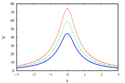
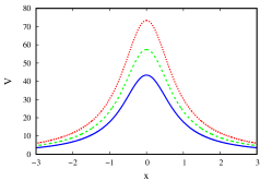
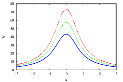
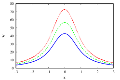
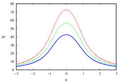
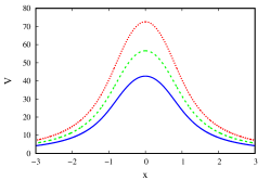
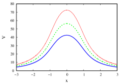
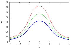
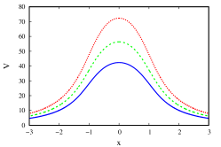
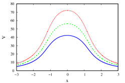
Figure 4: The potential of perturbation as a function of $x$ (the tortoise coordinate) for $l=6$ (blue), $l=7$ (green), $l=8$ (red). We have set $c=0.4$ (first row), $c=0.8$ (second row), $c=1.2$ (third row) and $c=1.6$ (fourth row). For each row we have $d=0.2$ (left panel), $d=0.6$ (center panel) and $d=1.4$ (right panel).

In Fig. 5 we show the imaginary part of the frequency as a function of the parameter $d$. For $c=0.4$ (first row), we note that the profile is monotonously increasing and approaches asymptotically to zero. In contrast, for $n=2$ and $n=3$, $Im(\omega)$ decreases with $d$, reach a minimum and grows again approaching asymptotically to zero. Particularly, for $l=6$, the frequency has positives values for $d\in(0.2,0.3)$ which means that the wormhole is unstable for this interval. For $c=0.8$ (second row), $c=1.2$ (third row) and $c=1.6$ (fourth row), $Im(\omega)$ is an increasing function and is always negative for the values of $d$ under consideration so the solution can be considered as stable under scalar perturbation for this parameters. We also note that the value of $Im(\omega)$ decreases as the overtone $n$ increases.

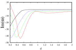
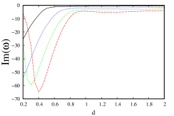
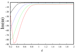
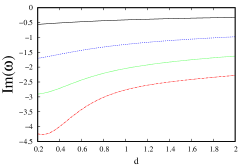
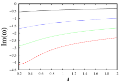
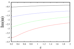
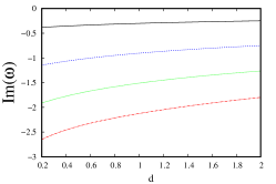
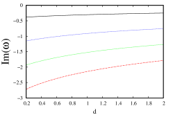
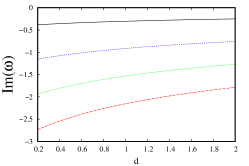
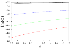
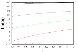
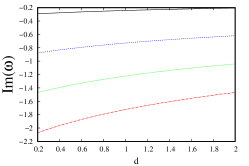
Figure 5: Imaginary part of the frequency as a function of $d$ for $n=0$ (black), $n=1$ (blue), $n=2$ (green), $n=3$ (red). We have set $c=0.4$ (first row), $c=0.8$ (second row), $c=1.2$ (third row) and $c=1.6$ (fourth row). For each row we have $l=6$ (left panel), $l=7$ (center panel) and $l=8$ (right panel).

In Fig. 6 we show the $Re(\omega)$ as a function of $d$ for different values of the parameter $c$. For $c=0.4$ (first row), the profile reaches a minimum located at different values of $d$ depending of the overtone. More precisely, as $n$ increases, the location of the minimum shift to larger values of $d$. Besides, except for $n=3$, the $Re(\omega)$ converge to the same value as $d$ grows which means that the oscillatory behaviour of the signal in indistinguishable for each overtone for large $d$. The asymptotic line shift to bigger values of $Re(\omega)$ as $l$ increases. For $c=0.8$ (second row) except for $n=0$ which remains constant, the $Re(\omega)$ reaches a maximum in contrast to the previous case. Moreover, the signal approaches asymptotically to a constant value which is different for each overtone. For $c=1.20$ (third row) and $l=6$, the signal is constant for $n=0$ and increases monotonously for $n=1$ and $n=2$ and reach a minimum for $n=3$. In contrast to the previous cases, the $Re(\omega)$ do not approach asymptotically to any value in the interval under consideration. For $l=7$ and $l=8$, except for the lowest overtone, $Re(\omega)$ increases monotonously. For $c=1.6$, the signal is constant for $n=0$, and increases monotonously for $n=1$ and $n=2$. For $n=3$, the signal increases with but undergoes some oscillatory behaviour for large $d$. This behaviour can be associated to numerical instabilities.

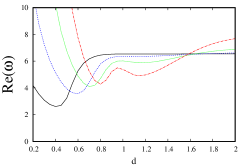
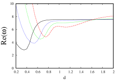
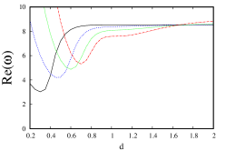
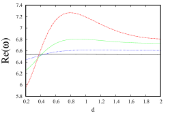
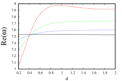
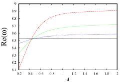
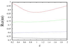
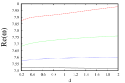
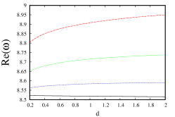
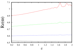
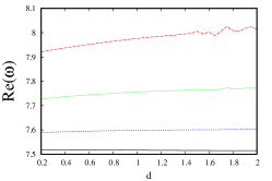
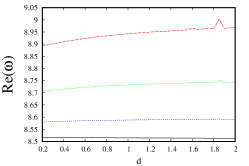
Figure 6: Real part of the frequency as a function of $d$ for $n=0$ (black), $n=1$ (blue), $n=2$ (green), $n=3$ (red). We have set $c=0.4$ (first row), $c=0.8$ (second row), $c=1.2$ (third row) and $c=1.6$ (fourth row). For each row we have $l=6$ (left panel), $l=7$ (center panel) and $l=8$ (right panel).

Based on the previous results, at this point some comments are in order. First, for $c=0.4$, the behaviour of signal for large $d$ is almost independent of the overtone. In particular, the damping factor, given by $e^{Im(\omega)}$, is almost the same for each $n$ under consideration. Similarly, the oscillatory behaviour is almost monochromatic: $Re(\omega)$ converge to the same value as $l$ grows. In this regard, if the main goal is to differentiate the behaviour from overtones for $c=0.4$, our model must be tested in the interval $d\in(0.2,1)$. It is worth mentioning that the model seems unstable in this interval for $n=3$. However, it is a well known fact that the model works well for lower overtones so that such instability could be associated to inaccuracy of the method. Second, for $c=0.8$ the behaviour clearly depends on the value of the overtone in the whole interval of $d$ under consideration. In particular, the damping is both stronger for large $n$ and weaker a $d$ grows. Regarding the $Re(\omega)$, the behaviour of the oscillatory part depends on the value of $d$. Indeed, $Re(\omega)$ decreases as $n$ grows in $d\in(0.2,0.4)$ but increases for large $n$ in $d\in(0.4,2)$. Interestingly, all the frequencies of the oscillatory part coincide for $d=0.4$. Finally, for $c=1.2$ and $c=1.6$, the pattern is clear: the damping is stronger as $n$ increases and $d$ decreases and the frequency of the oscillations grow as $n$ grows.

V Conclusions

In this work we obtained a traversable wormhole with vanishing radial tidal force by proposing a general embedding function with some free parameters. The parameters were reduced by imposing the basic requirements that must be satisfied by a wormhole geometry. In particular, we demanded the existence of a minimum radius (which defines the throat of the hole) and the flaring out condition. In order to explore how the geometry behaves in terms of the remaining parameter we analyzed both the quantifier of the exotic matter and the quasi normal modes of the solution. As a results, we observed that the solution requires a finite amount of exotic matter that decreases for certain values of the parameters involved. Besides, we obtained that in general the solution seems stable after scalar perturbations. Indeed, the imaginary part of the quasinormal frequencies remains negative which leads to a suitable damping factor for the signal.

References

- (1) M. S. Morris and K. S. Thorne. Wormholes in space-time and their use for interstellar travel: A tool for teaching general relativity. Am. J. Phys., 56:395–412, 1988.
- (2) M. S. Morris, K. S. Thorne, and U. Yurtsever. Wormholes, Time Machines, and the Weak Energy Condition. Phys. Rev. Lett., 61:1446–1449, 1988.
- (3) Miguel Alcubierre. Wormholes, Warp Drives and Energy Conditions, volume 189. Springer, 2017.
- (4) Matt Visser. Lorentzian wormholes: From Einstein to Hawking. 1995.
- (5) Francisco S. N. Lobo. Phantom energy traversable wormholes. Phys. Rev. D, 71:084011, 2005.
- (6) Remo Garattini. Casimir Wormholes. Eur. Phys. J. C, 79(11):951, 2019.
- (7) Zdeněk Stuchlík and Jaroslav Vrba. Epicyclic orbits in the field of Einstein–Dirac–Maxwell traversable wormholes applied to the quasiperiodic oscillations observed in microquasars and active galactic nuclei. Eur. Phys. J. Plus, 136(11):1127, 2021.
- (8) Kirill A. Bronnikov, Pavel E. Kashargin, and Sergey V. Sushkov. Magnetized Dusty Black Holes and Wormholes. Universe, 7(11):419, 2021.
- (9) Jose Luis Blázquez-Salcedo, Christian Knoll, and E. Radu. Einstein-Dirac-Maxwell wormholes: ansatz, construction and properties of symmetric solutions. 8 2021.
- (10) M. S. Churilova, R. A. Konoplya, Z. Stuchlik, and A. Zhidenko. Wormholes without exotic matter: quasinormal modes, echoes and shadows. JCAP, 10:010, 2021.
- (11) R. A. Konoplya and A. Zhidenko. Traversable Wormholes in General Relativity. Phys. Rev. Lett., 128(9):091104, 2022.
- (12) Francisco Tello-Ortiz, S. K. Maurya, and Pedro Bargueño. Minimally deformed wormholes. Eur. Phys. J. C, 81(5):426, 2021.
- (13) Cosimo Bambi and Dejan Stojkovic. Astrophysical Wormholes. Universe, 7(5):136, 2021.
- (14) Salvatore Capozziello, Orlando Luongo, and Lorenza Mauro. Traversable wormholes with vanishing sound speed in gravity. Eur. Phys. J. Plus, 136(2):167, 2021.
- (15) Jose Luis Blázquez-Salcedo, Christian Knoll, and Eugen Radu. Traversable wormholes in Einstein-Dirac-Maxwell theory. Phys. Rev. Lett., 126(10):101102, 2021.
- (16) Thomas Berry, Francisco S. N. Lobo, Alex Simpson, and Matt Visser. Thin-shell traversable wormhole crafted from a regular black hole with asymptotically Minkowski core. Phys. Rev. D, 102(6):064054, 2020.
- (17) Juan Maldacena and Alexey Milekhin. Humanly traversable wormholes. Phys. Rev. D, 103(6):066007, 2021.
- (18) Remo Garattini. Generalized Absurdly Benign Traversable Wormholes powered by Casimir Energy. Eur. Phys. J. C, 80(12):1172, 2020.
- (19) B. P. Abbott et al. Observation of Gravitational Waves from a Binary Black Hole Merger. Phys. Rev. Lett., 116(6):061102, 2016.
- (20) B. P. Abbott et al. GW151226: Observation of Gravitational Waves from a 22-Solar-Mass Binary Black Hole Coalescence. Phys. Rev. Lett., 116(24):241103, 2016.
- (21) Benjamin P. Abbott et al. GW170104: Observation of a 50-Solar-Mass Binary Black Hole Coalescence at Redshift 0.2. Phys. Rev. Lett., 118(22):221101, 2017. [Erratum: Phys.Rev.Lett. 121, 129901 (2018)].
- (22) Pablo Bueno, Pablo A. Cano, Frederik Goelen, Thomas Hertog, and Bert Vercnocke. Echoes of Kerr-like wormholes. Phys. Rev. D, 97(2):024040, 2018.
- (23) Vitor Cardoso, Seth Hopper, Caio F. B. Macedo, Carlos Palenzuela, and Paolo Pani. Gravitational-wave signatures of exotic compact objects and of quantum corrections at the horizon scale. Phys. Rev. D, 94(8):084031, 2016.
- (24) R. A. Konoplya and A. Zhidenko. Wormholes versus black holes: quasinormal ringing at early and late times. JCAP, 12:043, 2016.
- (25) Jose Luis Blázquez-Salcedo, Xiao Yan Chew, Jutta Kunz, and Dong-Han Yeom. Ellis wormholes in anti-de Sitter space. Eur. Phys. J. C, 81(9):858, 2021.
- (26) R. A. Konoplya and A. Zhidenko. Quasinormal ringing of general spherically symmetric parametrized black holes. 1 2022.
- (27) M. S. Churilova, R. A. Konoplya, and A. Zhidenko. Analytic formula for quasinormal modes in the near-extreme Kerr-Newman–de Sitter spacetime governed by a non-Pöschl-Teller potential. Phys. Rev. D, 105(8):084003, 2022.
- (28) R. A. Konoplya, A. F. Zinhailo, and Z. Stuchlik. Quasinormal modes and Hawking radiation of black holes in cubic gravity. Phys. Rev. D, 102(4):044023, 2020.
- (29) R. A. Konoplya and A. F. Zinhailo. Quasinormal modes, stability and shadows of a black hole in the 4D Einstein–Gauss–Bonnet gravity. Eur. Phys. J. C, 80(11):1049, 2020.
- (30) Roman A. Konoplya, C. Posada, Z. Stuchlík, and A. Zhidenko. Stable Schwarzschild stars as black-hole mimickers. Phys. Rev. D, 100(4):044027, 2019.
- (31) Angel Rincon, P. A. Gonzalez, Grigoris Panotopoulos, Joel Saavedra, and Yerko Vasquez. Quasinormal modes for a non-minimally coupled scalar field in a five-dimensional Einstein-power-Maxwell background. 12 2021.
- (32) Grigoris Panotopoulos and Ángel Rincón. Quasinormal spectra of scale-dependent Schwarzschild–de Sitter black holes. Phys. Dark Univ., 31:100743, 2021.
- (33) Ángel Rincón and Victor Santos. Greybody factor and quasinormal modes of Regular Black Holes. Eur. Phys. J. C, 80(10):910, 2020.
- (34) Ángel Rincón and Grigoris Panotopoulos. Quasinormal modes of an improved Schwarzschild black hole. Phys. Dark Univ., 30:100639, 2020.
- (35) Angel Rincon and Grigoris Panotopoulos. Quasinormal modes of black holes with a scalar hair in Einstein-Maxwell-dilaton theory. Phys. Scripta, 95(8):085303, 2020.
- (36) Wei Xiong, Peng Liu, Cheng-Yong Zhang, and Chao Niu. Quasi-normal modes of the Einstein-Maxwell-aether Black Hole. 12 2021.
- (37) Chao Zhang, Tao Zhu, and Anzhong Wang. Gravitational axial perturbations of Schwarzschild-like black holes in dark matter halos. Phys. Rev. D, 104(12):124082, 2021.
- (38) Grigoris Panotopoulos and Ángel Rincón. Quasinormal modes of five-dimensional black holes in non-commutative geometry. Eur. Phys. J. Plus, 135(1):33, 2020.
- (39) Chong Oh Lee, Jin Young Kim, and Mu-In Park. Quasi-normal modes and stability of Einstein–Born–Infeld black holes in de Sitter space. Eur. Phys. J. C, 80(8):763, 2020.
- (40) M. S. Churilova, R. A. Konoplya, and A. Zhidenko. Arbitrarily long-lived quasinormal modes in a wormhole background. Phys. Lett. B, 802:135207, 2020.
- (41) R. Oliveira, D. M. Dantas, Victor Santos, and C. A. S. Almeida. Quasinormal modes of bumblebee wormhole. Class. Quant. Grav., 36(10):105013, 2019.
- (42) Grigoris Panotopoulos and Ángel Rincón. Quasinormal modes of black holes in Einstein-power-Maxwell theory. Int. J. Mod. Phys. D, 27(03):1850034, 2017.
- (43) R. A. Konoplya, A. Zhidenko, and A. F. Zinhailo. Higher order WKB formula for quasinormal modes and grey-body factors: recipes for quick and accurate calculations. Class. Quant. Grav., 36:155002, 2019.
- (44) Matt Visser, Sayan Kar, and Naresh Dadhich. Traversable wormholes with arbitrarily small energy condition violations. Phys. Rev. Lett., 90:201102, 2003.
- (45) Bernard F. Schutz and Clifford M. Will. BLACK HOLE NORMAL MODES: A SEMIANALYTIC APPROACH. Astrophys. J. Lett., 291:L33–L36, 1985.