Large-momentum-transfer atom interferometers with $\mu$rad-accuracy using Bragg diffraction

Abstract

Large-momentum-transfer (LMT) atom interferometers using elastic Bragg scattering on light waves are among the most precise quantum sensors to date. To advance their accuracy from the mrad to the $\mu$rad regime, it is necessary to understand the rich phenomenology of the Bragg interferometer, which differs significantly from that of a standard two-mode interferometer. We develop an analytic model for the interferometer signal and demonstrate its accuracy using comprehensive numerical simulations. Our analytic treatment allows the determination of the atomic projection noise limit of an LMT Bragg interferometer, and provides the means to saturate this limit. It affords accurate knowledge of the systematic phase errors as well as their suppression by two orders of magnitude down to a few $\mu\mathrm{rad}$ using appropriate light pulse parameters.

Atom interferometery enables the most precise determination of the fine-structure constant [1, 2] as well as the most accurate quantum test of the universality of free fall [3]. The unique ability to perform absolute measurements of inertial forces [4] with high accuracy and precision makes atom interferometers prime candidates for real-world applications [5] like gravimetry [6, 7], gravity cartography [8], and inertial navigation [9, 10]. It has also recently led to the first measurement of the gravitational Aharonov-Bohm effect [11]. Large-momentum-transfer (LMT) beam splitting exploits the enhanced scaling of the interferometer sensitivity with the spatial separation of the coherent superposition of matter waves. Several proof-of-principle experiments have demonstrated record-breaking separations [12, 13, 14, 15] using various beam splitting techniques. LMT holds the potential for unprecedented precision of quantum sensors and will greatly facilitate our understanding of fundamental physics, e.g., through the detection of gravitational waves as well as the search for ultra-light dark matter [16, 17, 18, 19, 20, 21].

To date, all atom interferometers demonstrating metrological gain from LMT separations [1, 22, 11] use beam splitters based on the elastic scattering of atoms from time-dependent optical lattice potentials, i.e., Bragg diffraction [23, 24]. Compared to the standard picture of a two-mode interferometer, higher-order Bragg processes feature undesired diffraction orders [25, 26], see configuration (A) in Fig. 1, causing systematic uncertainties on the $\mathrm{mrad}$-level referred to as diffraction phase [27, 28, 13, 4, 29]. Yet, a comprehensive analytical model of Bragg interferometers is still missing.

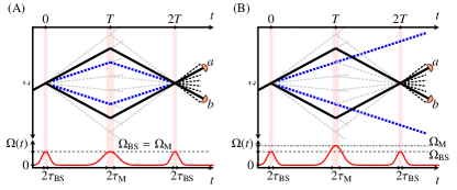
Figure 1: Mach-Zehnder (MZ) interferometer (solid trajectories) realized by $n$th-order Bragg beam splitters featuring parasitic paths and open ports (dashed lines), as shown in (A) and (B) in the inertial frame of the optical lattice. Imperfections arise from population of undesired diffraction orders and affect the atom numbers in the detected ports ${a},{b}$. Dominant parasitic paths for fifth-order of Bragg diffraction (thick dashed blue lines). Lower panels depict Gaussian pulse profiles $\Omega(t)$ equally spaced by an interrogation time $T$ and having individual pulse widths $\tau_{\mathrm{BS,M}}$. While peak values $\Omega$ are identical in (A), a tailored choice of $\Omega_{\mathrm{M}}$ enables the deflection of undesired paths and thus the suppression of the dominant parasitic interference effects in (B), see main text. In the following, we will refer to the depicted configurations as MZ types (A) and (B).

In this article, we present an analytical theory for atom interferometery that takes into account the multi-port as well as multi-path physics of Bragg diffraction. Using the popular Mach-Zehnder (MZ) geometry as an example, we present a conceptually straightforward way to suppress the diffraction phase simply by a suitable choice of pulse parameters. Indeed, a tailored combination of laser intensity and duration of the Bragg mirror pulse prevents the dominant parasitic paths from closing interferometers, as illustrated in Fig. 1(B). By largely suppressing the parasitic interferometer paths, the physics of the diffraction phase is dramatically simplified and reduces to a phase offset that can be readily determined. This way, we reduce the remaining diffraction phase below the $\mathrm{mrad}$-level for almost the entire range of beam splitter pulse parameters that yield diffraction losses $<10\%$, compatible with efficient high-order Bragg pulses [25, 26]. We verify the accuracy of our model by comparison to simulations of the MZ interferometer in numerical experiments.

In addition to the systematic effects, the complex contributions of parasitic paths and undetected, open ports in Bragg interferometers, depicted in Fig. 1, also affect their statistical properties. The statistical uncertainty is defined by the (Quantum) Cramér-Rao bounds ((Q)CRB) [30], which have not yet been determined for Bragg interferometers, although they modify the standard-quantum limit. We calculate the (Q)CRB and show that it exhibits a nontrivial dependence on the inevitable atom loss associated with Bragg diffraction. Moreover, we demonstrate that the phase estimation strategies we present in this work allow saturation of these fundamental bounds. Our detailed study of the atomic projection noise of efficient Bragg interferometers crucially establishes important design criteria for operating these devices at or below the standard quantum limit [31, 32, 33, 34].

Analytical model of Bragg MZ interferometer.— Bragg beam splitters and mirrors are generated by diffraction from an optical lattice potential $\displaystyle V(t)=2\hbar\Omega(t)\cos{(k\hat{z}-\delta t+\phi_{\mathrm{L}}(t))}$.

The lattice is pulsed by adjusting the intensity and relative frequencies, $\delta\equiv\omega_{1}-\omega_{2}$, of two counterpropagating light fields to coherently impart to the atoms a multiple of twice the photon recoil, $2n\hbar k$, and a lattice phase, $\phi_{\mathrm{L}}(t)$. The latter is determined by the relative phase between the two lattice laser fields. The integer $n$ denotes the Bragg order and the right choice of the velocity of the lattice $v_{\mathrm{L}}=\delta/k$ ensures resonance. Here, we focus on smooth Gaussian two-photon Rabi frequencies, $\Omega(t)=\Omega\,e^{-t^{2}/2\tau^{2}}$, reducing population of undesired diffraction orders [25]. Beam splitter and mirror operations can be realized with various combinations of peak Rabi frequency $\Omega$ and pulse width $\tau$ if they fulfill the respective condition on the pulse area [25, 26]. This freedom affords an optimized choice tailored to the experiment by balancing scattering to multiple diffraction orders against losses from velocity selectivity due to the Doppler effect [35, 26], predominant for short and long pulses, respectively.

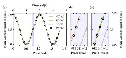
Figure 2: Signal phase scan. (a,b) Signal of MZ type (A) with $n=5$ in port ${a}$ scanned via the lattice phase $\phi_{\mathrm{L}}(t)=\phi_{\mathrm{L}}$ of the final beam splitter. We compare numerically simulated data $P^{\mathrm{meas}}_{a}(\phi)$ (symbols) to an ideal sinusoidal signal, $P^{\mathrm{ideal}}_{\mathrm{{a}}}(\phi)\equiv 1/2\cdot(1+\cos{(n\phi))}$ (gray solid line), and the analytical predictions of Eqs. (1) (orange dashed line) and Eq. (2) (green dotted line). Pulse parameters are $\Omega,\tau_{\mathrm{BS}},\tau_{\mathrm{M}}=28.5\omega_{\mathrm{r}},0.309\omega_{\mathrm{r}}^{-1},0.681\omega_{\mathrm{r}}^{-1}$, with $\omega_{\mathrm{r}}=\hbar k^{2}/2m$ being the recoil frequency of an atom with mass $m$. Beam splitter diffraction losses of $\approx 1.4\%$ amplify the signal distortions. (b) shows a bias phase shift of the ideal sinusoidal signal on the $\mathrm{mrad}$-level around mid fringe, i.e., $P_{a}(\phi)\approx 0.5$. In (c) mirror pulse parameters $\Omega_{\mathrm{M}},\tau_{\mathrm{M}}=31.8\omega_{\mathrm{r}},0.463\omega_{\mathrm{r}}^{-1}$ suppress dominant interference effects as illustrated in Fig. 1(B). This provides excellent agreement between the numerics and both analytical models in Eqs. (1) and Eq. (2).

In a MZ interferometer, two identical beam splitters and a mirror pulse generate and recombine out of a wave packet several copies of different momenta. The pulses are separated by an interrogation time $T$ and will be characterized in the following by $\Omega_{\mathrm{BS}},\tau_{\mathrm{BS}}$ and $\Omega_{\mathrm{M}},\tau_{\mathrm{M}}$.

Previously, we have modeled the physics of individual Bragg pulses by transfer matrices [26]. Here, we extend this treatment to also inlcude the dominant parasitic diffraction orders, see the Supplemental Material (SM). Transfer matrices that account for the diffraction operations and free propagation are combined to obtain the scattering matrix of a complete MZ interferometer $\mathcal{S}_{\mathrm{MZ}}(\phi,T,\Omega_{\mathrm{BS}},\tau_{\mathrm{BS}},\Omega_{\mathrm{M}},\tau_{\mathrm{M}})$, which, in addition to the parameters introduced above, depends on the metrological phase $\phi$ to be measured. Furthermore, we consider an incoming atomic ensemble with average momentum $-n\hbar k$ relative to the optical lattice and a Gaussian momentum width well below the lattice recoil $\sigma_{\!\!p}\ll\hbar k$, consistent with recently realized, ultracold Bose-Einstein condensate sources [36, 37], as initial state $\ket*{\psi^{\mathrm{in}}(\sigma_{\!\!p})}$. Putting the two together, we arrive at an expression for the output state $\ket*{\psi^{\mathrm{out}}(\phi,T,\Omega_{\mathrm{BS}},\tau_{\mathrm{BS}},\Omega_{\mathrm{M}},\tau_{\mathrm{M}},\sigma_{\!\!p})}=\mathcal{S}_{\mathrm{MZ}}\ket*{\psi^{\mathrm{in}}(\sigma_{\!\!p})}$. Its construction and explicit form are detailed in the SM.

From $\ket*{\psi^{\mathrm{out}}}$ follows the expected form of the signal for the relative atom numbers in the detected ports, $\displaystyle P_{{a}}(\phi)=N_{a}(\phi)/\left(N_{a}(\phi)+N_{b}(\phi)\right)$ and similarly for port ${b}$, cf. Fig. 1. In atom interferometry, the measurement of relative populations $P^{\mathrm{meas}}_{{a}}(\phi)$ ideally suppresses the statistical fluctuations of the initial atom number $N_{\mathrm{atoms}}$ in $\ket*{\psi^{\mathrm{in}}}$. Phase estimation usually requires scanning the phase $\phi$, e.g. via the control of the lattice phase $\phi_{\mathrm{L}}$ in the experiment, in order to fit the analytic model $P_{{a}}(\phi)$ to the interferometer signal $P^{\mathrm{meas}}_{{a}}(\phi)$. Subsequently, the inversion $P_{{a}}(\phi)$ yields the phase estimate $\phi^{\mathrm{est}}=P_{{a}}^{-1}(P^{\mathrm{meas}}_{{a}})$. Therefore, the quality of the model $P_{{a}}(\phi)$ crucially determines the systematic accuracy and the statistical sensitivity of the phase measurement, both of which we discuss below.

Interferometer including parasitic paths.— In an interferometer realized by higher-order Bragg pulses with a generic set of parameters $\Omega_{\mathrm{BS}},\tau_{\mathrm{BS}},\Omega_{\mathrm{M}},\tau_{\mathrm{M}}$, undesired diffraction orders will populate parasitic interferometer paths and open output ports illustrated in Fig. 1(A) to varying degrees. Their contributions to the interferometer signal can be significant and have been observed in experiments [38, 39, 40]. Our analytical model for $\ket{\psi_{\mathrm{out}}}$ reflects this in a signal for the relative atom number measurement, which takes the form of an infinite Fourier series,

$$P^{\mathrm{exact}}_{{a}}(\phi)=P_{0}+\sum^{\infty}_{j=1}A_{j}\cos{\left(j\,\phi+\varphi_{j}\right)}.$$ (1)

The amplitudes $A_{j}$ and phases $\varphi_{j}$ in Eq. (1) can be calculated as explained in the SM. We contrast this result with the standard model of an $n$-th-order Bragg MZ interferometer, which is obtained by idealizing the beam splitters and mirror as two-mode operations, $\displaystyle P^{\mathrm{ideal}}_{{a}({b})}(\phi)=P_{0}\pm A\cos{\left(n\phi\right)}$.

In Fig. 2(a,b) we demonstrate good agreement between the analytical signal of Eq. (1), taking into account the dominant parasitic paths for $n=5$, and data from numerical simulations. These are based on one-dimensional descriptions of the complete matter-wave interferometer in position space as per [41], whereby all diffraction orders are fully accounted for. In Fig. 2(a,b), we scan $\phi$ via the phase of the final beam splitting pulse, which we control by selecting a value for $\phi_{\mathrm{L}}=\phi_{\mathrm{L}}(t)$ for each data point. We consider an example of a set of pulses as in Fig. 1(A) with identical peak Rabi frequency, $\Omega=\Omega_{\mathrm{BS}}=\Omega_{\mathrm{M}}$, and durations that satisfy the corresponding pulse area conditions [25, 26] realizing efficient Bragg diffraction with about $1.4\%$ losses from the main paths per the first beam splitting pulse. Even for this small population of undesired diffraction orders, the sinusoidal signal of an ideal two-mode interferometer is inadequate and exhibits a diffraction phase shift of several mrad, cf. Fig. 2(b).

Evidence of undesired additional Fourier components contributing to the signal is found in [38, 39, 40], the origin of which can be understood as follows: (i) Figure 1 makes evident that the multi-port nature of the Bragg beam splitters and the associated interference render the combined atom number in the detected ports ${a}$ and ${b}$, $N_{a}(\phi)+N_{b}(\phi)=N_{\mathrm{atoms}}-N_{\mathrm{open}}(\phi)$, phase-dependent. Here, $N_{\mathrm{open}}(\phi)\big{)}$ denotes the population of all undetected (open) output ports, cf. Fig. 1. This is in contrast to an ideal two-mode interferometer, where $N_{a}(\phi)+N_{b}(\phi)$ simply amounts to the total number of atoms $N_{\mathrm{atoms}}$. Accordingly, the relative atom numbers in a Bragg interferometer, $\displaystyle N_{{a}({b})}(\phi)/\big{(}N_{\mathrm{atom}}-N_{\mathrm{open}}(\phi)\big{)}$, will be a ratio of $\phi$-dependent functions and therefore in general contain Fourier components of any order. (ii) In addition, the functional dependence of the absolute atom numbers $N_{{a},{b}}(\phi)$ is also complicated by the occurrence of parasitic interferometers. For the example of the MZ interferometer in Fig. 1(A) parasitic MZ terms (cf. [38]) arise, when undesired diffraction orders overlap with the main interferometry arms at $t=2T$. In particular, this causes $A_{j}$ and $\varphi_{j}$ to depend on the interrogation time $T$, in addition to the parameters of the individual Bragg pulses, as observed in [38, 39]. Notwithstanding its correctness, it will be challenging to apply the waveform in Eq. (1) due to the large number of parameters involved and the limited control over them.

Interferometer with suppressed parasitic paths.— A simple way to efficiently suppress interference with the dominant parasitic paths in the MZ geometry is to design the mirror pulse to be approximately transparent to them, as illustrated in Fig. 1(B). Specific combinations $\Omega_{\mathrm{M}},\tau_{\mathrm{M}}$ achieving this for $n=5$ are stated in the SM but they do in fact exist for all relevant higher orders of Bragg diffraction, except $n=2$. It is straightforward to omit the influence of parasitic paths in our analytical model and consider only the effects of the open ports (point (i) above). Doing so simplifies the signal of the MZ interferometer in ports ${a}$ and ${b}$ to

$$\begin{split}P_{{a}({b})}(\phi)&=P_{0}\pm\sum^{3}_{j=1}A_{j}\sin{\left(j\cdot\left(n\phi+\gamma+\frac{\pi}{2}\right)\right)}+\mathcal{O}[\gamma^{3}],\end{split}$$ (2)

where $P_{{b}}(\phi)$ is shifted by $\pi$ relative to $P_{{a}}(\phi)$ as one would expect, see SM. In contrast to Eq. (1) this expression contains only the harmonics of a single Fourier component $n\phi$, and a phase shift $\gamma$ common to all harmonics. Moreover, we can show that this shift is independent of $T$ and can be calculated for given beam splitter parameters $\Omega_{\mathrm{BS}},\tau_{\mathrm{BS}}$, see SM. In fact, $\gamma$ is a small parameter closely related to the losses to undesired diffraction orders during beam splitting [26]. For an interferometer with suppressed parasitic paths as in Fig. 1(B), both the exact signal in Eq. (1) and the much simpler formula in Eq. (2) are in excellent agreement with the data from a numerical simulation, as can be seen in Fig. 2(c).

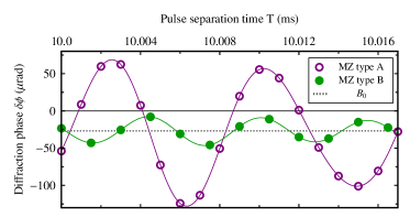
Figure 3: Phase estimation error. We evaluate the diffraction phase $\delta\phi$ in Eq. (3) using numerical simulations of MZ interferometers of types (A) and (B) with $n=5$. $\delta\phi$ is determined at mid fringe $\phi=\frac{3\pi}{2}\frac{1}{5}$ and beam splitters are chosen to operate at a so-called ’magic’ Bragg duration minimizing individual diffraction losses to $\approx 0.18\%$ (see main text). This reduces oscillations in $\delta\phi$ to the $\mu\mathrm{rad}$-level while scanning the pulse separation time $T$ (cf. [38, 39]). The first data set (open circles) has been obtained for parameters $\Omega,\tau_{\mathrm{BS}},\tau_{\mathrm{M}}=30.75\omega_{\mathrm{r}},0.218\omega_{\mathrm{r}}^{-1},0.519\omega_{\mathrm{r}}^{-1}$, with $\omega_{\mathrm{r}}=\hbar k^{2}/2m$ being the recoil frequency of an atom with mass $m$. Suppressing dominant parasitic interference effects via $\Omega_{\mathrm{M}},\tau_{\mathrm{M}}=31.8\omega_{\mathrm{r}},0.463\omega_{\mathrm{r}}^{-1}$ (closed circles, case (B)) further reduces the oscillation amplitude by a factor of five to $<40\,\mu\mathrm{rad}$. Solid lines represent fits to the data explained in the main text, the offset of which is the effectively same $B_{0}\approx-27\,\mu\mathrm{rad}$ (dotted) for both data sets.

Diffraction phase.— We proceed to quantify the diffraction phase [28, 39], i.e., the systematic deviation of the model in Eq.  (2) from the actual signal obtained in numerical simulations. We compare its application to the signal of interferometers (A) without and (B) with suppression of parasitic paths, as in Fig. 1(A) and (B) respectively. The deviation between the phase and its estimate $\phi^{\mathrm{est}}=P_{{a}}^{-1}(P_{a}^{\mathrm{meas}})$ is

$$\delta\phi=P_{{a}}^{-1}(P_{a}^{\mathrm{meas}})-\phi=\left.P_{{a}}^{-1}(P_{a}^{\mathrm{meas}})\right|_{\gamma=0}-\phi-\frac{\gamma}{n}.$$ (3)

Here, we emphasize the fact, that $\gamma$ is a shift common to all Fourier components in Eq. (2), which we have taken advantage of in the second equality. The error $\delta\phi$ in determining the actual phase $\phi$ depends on the knowledge of the value of $\gamma$ and the accuracy of the model with respect to the remaining phase, $\left.P_{{a}}^{-1}(P_{a}^{\mathrm{meas}})\right|_{\gamma=0}$. Since $\gamma$ can be inferred quite accurately for given beam splitter parameters (cf. SM) it is the latter contribution which sets the systematic uncertainty. Furthermore, the scaling $n\phi$ in Eq. (2) highlights, that both contributions to the diffraction phase in Eq. (3) will be linearly suppressed by the order $n$ of the Bragg pulses, cf. [28].

We extract $\delta\phi$ after fitting the analytical model Eq. (2) to signals $P_{a}^{\mathrm{meas}}$ generated in numerical simulations and plot it in Fig. 3 against the pulse separation time $T$ for interferometers of type (A) and (B). In both realizations of the MZ geometry with fifth-order Bragg pulses, spurious MZ interference terms cause oscillations at frequencies $(5\pm 1)\omega_{\mathrm{r}}$, which are related to the recoil frequency $\omega_{\mathrm{r}}=\hbar k^{2}/2m$ via the kinematic phases of the main interferometer arms relative to the main parasitic diffraction orders, cf. [38, 39]. Here, $m$ is the mass of the atom. This is despite minimizing beam splitter losses to about $0.18\%$ via our selection of pulse parameters, referred to by Parker et al. as a ’magic’ Bragg duration, which effectively reduces the $T$-dependence of the diffraction phase in the $n=5$ conjugated Ramsey-Bordé interferometer discussed in Ref. [39]. We can use a fit model $f(T)=B_{0}+B_{1}\cos{\left(4\omega_{\mathrm{r}}T+\eta_{1}\right)}+B_{2}\cos{\left(6\omega_{\mathrm{r}}T+\eta_{2}\right)}$ to extract the amplitude offset $B_{0}$ and the peak-to-peak value $\mathrm{PP}\equiv\absolutevalue{\max\nolimits_{\forall T}f(T)-\min\nolimits_{\forall T}f(T)}$ of the oscillations in the diffraction phase. For the pulse parameters assumed in Fig. 3, the offset $B_{0}\approx-27\,\mu\mathrm{rad}$ is the same for both cases (A) without and (B) with suppression of parasitic paths. This shows, that the inclusion of $\gamma/n\approx 280\,\mu\mathrm{rad}$ in Eq. (3) accounts for most of the $T$-independent shift. However, $\mathrm{PP}$ values of both data sets are very different, lying in the range of 200 $\mu$rad for (A) and about 40 $\mu$rad for (B). This reduction is significant because the net diffraction phase shift may be on the order of the PP value due to insufficient control over the separation time $T$ at the $\mu$s level or, if $T$ is sampled, due to aliasing effects, cf. [39].

The offset $|B_{0}|$ and the $\mathrm{PP}$ value of the oscillations in the diffraction phase are given in Fig. 4(a,b) for a range of parameters $\Omega_{\mathrm{BS}},\tau_{\mathrm{BS}}$, which we restrict by requiring beam splitter losses of less than $10\%$. We again compare both Bragg mirror pulse configurations (A) and (B). Figure 4(a) confirms that through the inclusion of $\gamma$ in Eq. (2) we achieve a residual $T$-independent contribution to the diffraction phase $\delta\phi$ of at most a few tenths of $\mu\mathrm{rad}$ for both Bragg mirror configurations. At the same time, Fig. 4(b) highlights that the oscillations of $\delta\phi$ can be on the order of several $\mathrm{mrad}$ and are therefore comparable to $\gamma/n$, see SM, in case of pulse parameters with relatively strong couplings to undesired diffraction orders. As implied by Fig. 4(c), the behavior of both quantities characterizing $\delta\phi$ is directly related to the losses in beam splitter operations. Notably, the local minimum indicates the magic Bragg duration for fifth-order Bragg beam splitters mentioned earlier but in fact, such minima exist for all orders $n>1$ and are a feature predicted by Landau-Zener theory [26].

We conclude that the diffraction phase of MZ Bragg interferometers can be suppressed by means of the Bragg mirror pulse below $1~{}\mathrm{mrad}$ for most parameters $\Omega_{\mathrm{BS}},\tau_{\mathrm{BS}}$ and even down to a few $\mu\mathrm{rad}$ for sufficiently long beam splitter durations. In contrast, without suppression of parasitic paths and without account for the diffraction phases (including $\gamma$) by means of Eq. (2), the accuracy would be limited to more than $0.5~{}\mathrm{mrad}$ in the same regime, which constitutes an improvement by two orders of magnitude. The remaining diffraction phase is limited by higher-order contributions in $\gamma$ and the finite efficiency in suppressing parasitic paths.

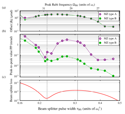
Figure 4: Diffraction phase suppression in MZ geometry. (a,b) Fits to Eq. (3) are evaluated for numerical MZ signals recorded over scans of $T\in[10,10.016]~{}\mathrm{ms}$ as shown in Fig. 3(a) using pulse parameter respecting the condition on the Bragg pulse area [25, 26]. Closed (open) symbols represent data with (w/o) suppression of parasitic paths parameterized via $\Omega=\Omega_{\mathrm{BS}},\tau_{\mathrm{BS}}$. (a) shows absolute values of the residual offset $|B_{0}|\leq 30\,\mu\mathrm{rad}$ (symbols) independent of the mirror pulse. (b) The adapted mirror pulse (case (B)) significantly suppresses PP values for most parameters below $1~{}\mathrm{mrad}$ and to less than $10~{}\mu\mathrm{rad}$ for sufficiently long beam splitter pulse durations. Lines connecting the data points serve as guides to the eye. (c) Numerically obtained population loss from the main diffraction orders $\ket{\pm 5\hbar k}$ of a single beam splitter. Results in Fig. 2 (Fig. 3) use parameters corresponding to the visible local maximum (minimum) denoted by the solid (dotted) vertical line.

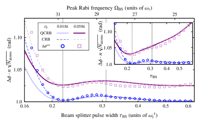
Figure 5: Sensitivity bound of multi-port Bragg interferometers with uncorrelated particles. Cramér-Rao bound (CRB, dashed lines) and Quantum Cramér-Rao bound (QCRB, solid lines) for a fifth-order Bragg MZ interferometer in configuration (B). Upon scanning $\Omega_{\mathrm{BS}},\tau_{\mathrm{BS}}$ we suppress the dominant parasitic interferometery paths using pulse parameters $\Omega_{\mathrm{M}},\tau_{\mathrm{M}}=31.8\omega_{\mathrm{r}},0.463\omega_{\mathrm{r}}^{-1}$. Both bounds are shown for momentum spread $\sigma_{\!\!p}=0.01\hbar k~{}(0.05\hbar k)$ in blue (purple) and scaled to the projection noise limit of an ideal two-mode MZ, $n\sqrt{N_{\mathrm{atoms}}}$. Symbols represent the statistical uncertainty $\Delta\phi^{\mathrm{est}}$ of a phase estimate based on Eq. (2) at mid fringe obtained for numerical simulations. We set $\phi=\frac{3\pi}{2}\frac{1}{5}$ for both the CRB and for $\Delta\phi^{\mathrm{est}}$ and fix the time $T=10~{}\mathrm{ms}$. The statistical uncertainty operated with equal Peak Rabi frequencies (case (A) in inset) suffers from increased finite-velocity Doppler effects.

Phase sensitivity.— To complete our study of the model in Eq. (2), we discuss the statistical uncertainty of the phase estimate $\phi^{\mathrm{est}}=P_{{a}}^{-1}(P_{a}^{\mathrm{meas}})$, which is given by the projection noise $\Delta\phi^{\mathrm{est}}\approx\sqrt{\frac{P_{a}(\phi)(1-P_{a}(\phi))}{N_{a}(\phi)+N_{b}(\phi)}}\frac{1}{\absolutevalue{\partial_{\phi}P_{a}(\phi)}}$, cf. SM. We emphasize that this is quite different from the projection noise of an ideal two-mode MZ-Bragg interferometer, which is $\Delta\phi^{\mathrm{est}}=\frac{\sqrt{P_{0}(1-P_{0})}}{n\,A\sqrt{N_{\mathrm{atoms}}}}$ at mid fringe, where again $N_{\mathrm{atoms}}$ denotes the number of atoms entering the interferometer. We benchmark the achievable phase sensitivity by the CRB and the QCRB, both of which follow from the analytical expression for $\ket*{\psi^{\mathrm{out}}}$, cf. SM. The CRB sets the projection noise limit when measuring relative atom numbers in the main ports ${a},{b}$, as depicted in Fig. 1. The QCRB bounds the projection noise for arbitrary measurements performed on all output ports of the final Bragg beam splitter.

The results are shown in Fig. 5 for MZ interferometers of type (B) and, in the inset, for (A) for the same range of beam splitter parameters considered in Fig. 4. First of all, we observe that $\Delta\phi^{\mathrm{est}}$ for phase estimation based on Eq. (2) using numerical data agrees well with the analytical CRB and QCRB. The visible deviations are on the level to be expected due to our perturbative treatment of finite velocity effects and beam splitter losses, cf. SM. We show the phase sensitivity in Fig. 5 scaled to $n\sqrt{N_{\mathrm{atoms}}}$, i.e., the CRB of an ideal two-mode interferometer with $P_{0}=A=1/2$. This reveals that the projection noise limit for a Bragg interferometer lies a few percent above this value. The increase of the CRB with growing momentum spread $\sigma_{\!\!p}$ is caused by atom losses due to velocity selectivity of the Bragg process, which become stronger for longer pulse durations, cf. [35]. In addition, as revealed by our two choices of velocity width, velocity selectivity is reduced for case (B) because of the relatively short mirror pulse duration for the suppression of parasitic paths, see SM. The loss of sensitivity at shorter beam splitter pulse durations is due to the increasing non-adiabaticity of Bragg diffraction and the associated diffraction losses [26], see Fig. 4(c). Interestingly, there is no discernible difference in performance between either configuration despite deliberately deflecting atoms out of the interferometer in scenario (B), see Fig. 1(B). The reason being, that Bragg diffraction losses primarily populate parasitic interferometers with scale factors smaller than the main diffraction order (here, $n=5$). Accordingly, their contributions effectively decrease the space-time area and thus increase the statistical uncertainty of the phase measurement. Overall, best sensitivity is achieved at the local minimum of beam splitting losses from the main diffraction orders $\pm 5\hbar k$, cf. Fig. 4(c). This sets the fundamental projection noise limit of a Bragg atom interferometer.

Conclusions.— In summary, we have presented an analytical model for LMT atom interferometers based on Bragg diffraction, which permits a thorough understanding of their systematic and statistical uncertainties and their fundamental sensitivity bounds. Our model provides design criteria for reaching these bounds and paves the way towards accuracies in the $\mu$rad-range using higher-order Bragg diffraction in combination with ultra-cold atomic sources [36, 37]. The operation of LMT interferometers at or near the limit of quantum projection noise is a critical requirement if they are to be combined with entangled sources [33, 34]. The methods and techniques developed here are general and can be applied also to other interferometer topologies, such as the conjugated Ramsey-Bordé interferometer in [1], and to other diffraction techniques as, e.g., double Bragg diffraction pulses [42, 43, 44]. Our work contributes to the development of high-precision quantum sensors for fundamental tests and towards atom interferometers fulfilling the size, weight, and power (SWaP) requirements of modern real-world applications [4, 29], especially in combination with resonator-enhanced light fields [45].