Modeling Network-level Traffic Flow Transitions on Sparse Data

Abstract.

Modeling how network-level traffic flow changes in the urban environment is useful for decision-making in transportation, public safety and urban planning. The traffic flow system can be viewed as a dynamic process that transits between states (e.g., traffic volumes on each road segment) over time. In the real-world traffic system with traffic operation actions like traffic signal control or reversible lane changing, the system’s state is influenced by both the historical states and the actions of traffic operations. In this paper, we consider the problem of modeling network-level traffic flow under a real-world setting, where the available data is sparse (i.e., only part of the traffic system is observed). We present DTIGNN, an approach that can predict network-level traffic flows from sparse data. DTIGNN models the traffic system as a dynamic graph influenced by traffic signals, learns the transition models grounded by fundamental transition equations from transportation, and predicts future traffic states with imputation in the process. Through comprehensive experiments, we demonstrate that our method outperforms state-of-the-art methods and can better support decision-making in transportation.

1. Introduction

Modeling how network-level traffic flow changes in the urban environment is useful for decision-making in various applications, ranging from transportation (Lin et al., 2018; Fu et al., 2020), public safety (Wang et al., 2017; Zhang et al., 2017) to urban planning (Jayarajah et al., 2018). For example, modeling the network-level traffic flow can help build a good simulator and serve as a foundation and a testbed for reinforcement learning (RL) on traffic signal control (Wei et al., 2018), routing (Wang et al., 2019) and autonomous driving (Wu et al., 2018).

The modeling of the traffic flow system can be viewed as a dynamic process that transits from state $s_{t}$ to state $s_{t+1}$. The state of the system can include traffic conditions like traffic volume, average speed, etc. The ultimate objective to build a real predictor is to minimize the error between estimated state $\hat{s}_{t+1}$ and true state observation $s_{t+1}$. Traditional transportation approaches assume the state transition model is given and calibrate parameters accordingly using observed data (Kotsialos et al., 2002; Boel and Mihaylova, 2006; Wang et al., 2022; Oh et al., 2018). However, the assumption on the state transition model is often far from the real world because the real-world system is a highly complex process, especially for the system in which humans are key players.

Recently, growing research studies have developed data-driven methods to model state transitions. Unlike traditional transportation approaches, data-driven methods do not assume the underlying form of the transition model and can directly learn from the observed data. With the data-driven methods, a more sophisticated state transition model can be represented by a parameterized model like neural nets and provides a promising way to mimic the real-world state transitions. These data-driven models predict the next states based on the current state and historical states with spatial information, through deep neural networks like Recurrent Neural Network (RNN) (Yao et al., 2018; Yu et al., 2017b) or Graph Neural Network (GNN)  (Kim et al., 2020; Li et al., 2017; Song et al., 2020; Wang et al., 2020; Wu et al., 2020; Zhang et al., 2020a; Zhao et al., 2019; Guo et al., 2019; Fang et al., 2021). As shown in Figure 1(a), these methods focus on directly minimizing the error between estimated state $s_{t+1}$ and true observed state $s_{t+1}$, with an end-to-end prediction model $P$. Although having shown great effectiveness over traditional methods, these approaches face two major challenges:

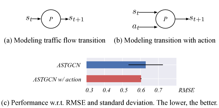
Figure 1. Two perspectives in modeling traffic flow. (a) Existing data-driven models directly predict the next state $s_{t+1}$ based on its past states with a model $P$. (b) Modeling the traffic state transition takes both past states and traffic management actions. (c) The method with traffic management actions as input (ASTGCN (Guo et al., 2019) w/ action) shows better performance.

$\bullet$ The influence of traffic management actions. In the real-world traffic system with traffic management actions like traffic signal control or reversible lane changing, the system’s state is influenced not only by its previous states, but more importantly, by the actions of traffic management actions. Simply taking previous states (e.g.., volumes) as input may cause conflicting learning problems. For example, given a road segment $A$ with $K$ vehicles at time $t$, the road segment has traffic signals at its end, controlling whether the vehicles can leave the road or not. When $A$ is having green light, the future traffic volume on the road is likely to drop, but if $A$ is having red light, the future traffic volume is likely to rise. When the model only considers historical traffic volumes, the conflicting traffic volume will confuse the learning process. As a result, the learned model is likely to predict $s_{t+1}$ with a large error or variance. As is shown in Figure 1, if we take the traffic management actions (e.g., how traffic signal changes) into consideration, the traffic flow will be predicted more accurately. To the best of our knowledge, none of the existing literature has integrated traffic actions into data-driven models.

It is worth noting that modeling the traffic flow state transition with traffic management actions is more than improving the prediction accuracy. A well-trained state transition model with traffic management actions can be utilized to provide actionable insights: it can be used to find the best decision to mitigate the problems in traffic flow system (e.g., traffic congestion), and then on prescribing the best actions to implement such a decision in the physical world and study the impact of such implementation on the physical world.

$\bullet$ The sparsity of traffic data. In most real-world cases, the available observation is sparse, i.e., the traffic flow states at every location are difficult to observe. It is infeasible to install sensors for every vehicle in the road network or to install cameras covering every location in the road network to capture the whole traffic situation. Most real-world cases are that the camera data usually only covers some intersections of the city, and the GPS trajectories may only be available on some cars, like taxis. As data sparsity is considered as a critical issue for unsatisfactory accuracy in machine learning, directly using datasets with missing observations to learn the traffic flow transitions could make the model fail to learn the traffic situations at the unobserved roads.

To deal with sparse observations, a typical approach is to infer the missing observations first (García-Laencina et al., 2010; Batista et al., 2002; Li et al., 2019; Luo et al., 2018; Yoon et al., 2018; Qin et al., 2021) and then learn the model with the transition of traffic states. This two-step approach has an obvious weakness, especially in the problem of learning transition models with some observations entirely missing. For example, mean imputation (García-Laencina et al., 2010) is often used to infer the missing states on the road by averaging the states from nearby observed roads. However, not all the traffic from nearby roads would influence the unobserved road because of traffic signals, making the imputed traffic states different from the true states. Then training models on the inaccurate data would further lead to inaccurate predictions. A better approach is to integrate imputation with prediction because they should inherently be the one model: the traffic state on the unobserved road at time $t$ is actually influenced by the traffic flows before $t$, including the flows traversed from nearby roads and the remaining flows of its own, which is also unobserved and needs inference.

In this paper, we present DTIGNN, a GNN-based approach that can predict network-level traffic flows from sparse observations, with Dynamic adjacency matrix, Transition equations from transportation, and Imputation. To model the influence of traffic management actions, DTIGNN represents the road network as a dynamic graph, with the road segments as the nodes, road connectivity as the edges, and traffic signals changing the road connectivity from time to time. To deal with the sparse observation issue, we design a Neural Transition Layer to incorporate the fundamental transition equations from transportation, with theoretical proof on the equivalence between Neural Transition Layer and the transportation equations. DTIGNN further imputes the unobserved states iteratively and predict future states in one model. The intuition behind is, the imputation and prediction provided by data-driven models should also follow the transition model, even though some flows are unobservable.

We conduct comprehensive experiments using both synthetic and real-world data. We demonstrate that our proposed method outperforms state-of-the-art methods and can also be easily integrated with existing GNN-based methods. The ablation studies show that the dynamic graph is necessary, and integrating transition equation leads to an efficient learning process. We further discuss several interesting results to show that our method can help downstream decision-making tasks like traffic signal control.

2. Related Work

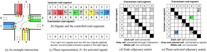
Figure 2. Illustration of traffic signals and their influence on the connectivity between road segments. (a) An intersection with eight connecting road segments and traffic signals. (b) The signals set and their controlled road segments in the example, with right-turn signals illustrated in grey cells. (c) The phase representation for the activated signals in the example intersection.(d) The static adjacency matrix between road segments induced by road network structure. (e) the dynamic adjacency matrix induced by traffic signals. Best viewed in color.

Traffic Prediction with Deep Learning. Recently, many efforts have been devoted to developing traffic prediction techniques based on various neural network architectures. One straightforward solution is to apply the RNN, or convolutional networks (CNN) to encode the temporal (Yu et al., 2017a; Liu et al., 2016) and spatial dependency (Zhang et al., 2017; Yao et al., 2018, 2019). Recent works introduce GNN to learn the traffic networks (Zhang et al., 2020a). DCRNN (Li et al., 2017) utilizes the bi-directional random walks on the traffic graph to model spatial information and captures temporal dynamics by RNN. Transformer models (Wang et al., 2020; Kim et al., 2020; Wu et al., 2020; Zhao et al., 2019; Zhang et al., 2020b) utilize spatial and temporal attention modules in transformer for spatial-temporal modeling. STGCN (Yu et al., 2017b) and GraphWaveNet (Wu et al., 2019) model the spatial and temporal dependency separately with graph convolution and 1-D convolution. Later studies (Song et al., 2020; Guo et al., 2019) attempt to incorporate spatial and temporal blocks altogether by localized spatial-temporal synchronous graph convolution module regardless of global mutual effect. However, when predicting traffic states, all the previous GNN-based models assume that the node feature information is complete, which is unfeasible in real-world cases. Our work can be easily integrated into these GNN-based methods and handle incomplete and missing feature scenarios, which have not been well explored in existing solutions.  
 Traffic Inference with Missing Data. Incomplete and missing data is common in real-world scenario. In machine learning area, imputation techniques are widely used for data completion, such as mean imputation (García-Laencina et al., 2010), matrix factorization (Koren et al., 2009; Mazumder et al., 2010), KNN (Batista et al., 2002) and generative adversarial networks (Li et al., 2019; Luo et al., 2018; Yoon et al., 2018). However, general imputation methods are not always competent to handle the specific challenge of spatial and temporal dependencies between traffic flows, especially when traffic flows on unmonitored road segments are entirely missing in our problem setting.

Many recent studies (Tang et al., 2019; Yi et al., 2019) use graph embeddings or GNN to model the spatio-temporal dependencies in data for network-wide traffic state estimation. Researchers further combine temporal GCN with variational autoencoder and generative adversarial network to impute network-wide traffic state (Qin et al., 2021). However, most of these methods assume the connectivity between road segments is static, whereas the connectivity changes dynamically with traffic signals in the real world. Moreover, all the graph-based methods do not explicitly consider the flow transition between road segments in their model. As a result, the model would likely infer a volume for a road segment when the nearby road segments do not hold that volume in the past.

3. Preliminaries

Definition 3.1 (Road network and traffic flow).

A road network consists of road segments, intersections, and traffic signals. Road segments are connected through intersections, and their connectivity changes with the action of traffic signals. The traffic flow on a road segment is directional, with incoming traffic flow from several upstream road segments, and different outgoing traffic flows to downstream road segments.

Definition 3.2 (Traffic signal action $p$).

The traffic signal action $p_{t}\in\{0,1\}^{P}$ represents a traffic signal phase (Wei et al., 2019) at time $t$, where there are $P$ signals in total, and its $k$-th value $p_{t}[k]=1$, indicating the signal is green, and corresponding traffic flows are allowed to travel from upstream roads to downstream roads.

Definition 3.3 (Road adjacency graph $\mathcal{G}$).

We represent the road network as a directed dynamic graph $\mathcal{G}_{t}=\{\mathcal{R},\mathcal{A}_{t}\}$ at time $t$, where $\mathcal{R}=\{r^{1},...,r^{N}\}$ is a set of $N$ road segments and $\mathcal{A}_{t}\in\mathbb{R}^{N\times N}$ is the adjacency matrix indicating the connectivity between road segments at time t. In this paper, $\mathcal{A}_{t}$ is dynamically changing with time $t$ due to the actions of traffic signals.

Figure 2(a) shows an example intersection. Figure 2(b) indicates the intersection has 12 different signals, each of which changes the traffic connectivity from the upstream road segments to corresponding the downstream roads. Now the intersection is at signal phase $p_{t}$. In Figure 2(c), $p_{t}[0]=1$ denotes that traffic flows can move from the upstream road $\#1$ to downstream road $\#8$. A static adjacency matrix is constructed based on the road network topology, and a dynamic adjacency matrix can be constructed based on the connectivity of between upstream and downstream road segments with signal phases.

Definition 3.4 (Observability mask M).

In real-world traffic systems, some road segments are unobserved for the entire time due to the lack of sensors. We denote the observability of traffic states as a static binary mask matrix $\textbf{M}\in\{0,1\}^{N\times F}$, and $F$ is the length of a state feature (also called channels), where $F=3$ when the road has three outgoing flows. When the road segment is observed, $\textbf{M}^{i}=\textbf{1}^{F}$; when the road segment is unobserved, $\textbf{M}^{i}=\textbf{0}^{F}$.

Definition 3.5 (Graph state tensor $\mathcal{X}$, observed $\dot{\mathcal{X}}$, unobserved $\ddot{\mathcal{X}}$, predicted $\widehat{\mathcal{X}}$, merged $\mathcal{X}^{\prime}$).

We use $\textbf{x}_{t}^{i}\in\mathbb{R}^{F}$ to denote the traffic volumes on road $r^{i}\in\mathcal{R}$ at time $t$. $\textbf{X}_{t}=(\textbf{x}_{t}^{1},\textbf{x}_{t}^{2},\cdots,\textbf{x}_{t}^{N})\in\mathbb{R}^{N\times F}$ denotes the states of all the road segments at time $t$, including the observed part $\dot{\textbf{X}}_{t}=\textbf{X}_{t}\odot\textbf{M}$ and unobserved part $\ddot{\textbf{X}}_{t}=\textbf{X}_{t}\odot(\textbf{1}-\textbf{M})$, where $\odot$ is the element-wise multiplication. The graph state tensor $\mathcal{X}=(\textbf{X}_{1},\textbf{X}_{2},\cdots,\textbf{X}_{T})\in\mathbb{R}^{N\times F\times T}$ denotes the states of all the road segments of all time, with $\dot{\mathcal{X}}=(\dot{\textbf{X}}_{1},\dot{\textbf{X}}_{2},\cdots,\dot{\textbf{X}}_{T})$ as observed state tensor and $\ddot{\mathcal{X}}$ as unobserved state tensor. The predicted values of $\mathcal{X}$ will be denoted with $\widehat{\mathcal{X}}$, and the merged values for $\mathcal{X}$ will be denoted as $\mathcal{X}^{\prime}$.

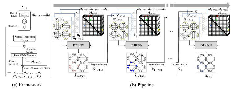
Figure 3. Model framework and training pipeline. (a) The framework of DTIGNN network. The network can be built upon exiting spatial-temporal GNNs with our Attention based Spatial-Temporal GNNs Layer appended after existing GNNs. (b) The training pipeline of DTIGNN. One training round goes through data in an auto-regressive way, and the predictions from previous time steps are used as imputations to update the unobserved data at the current time step.

Problem 1 (Traffic Flow Transition Modeling).

Based on the definitions above, the modeling of traffic flow transition is formulated as: given the observed tensor $\dot{\mathcal{X}}$ on a road adjacency graph $\mathcal{G}$, the goal of modeling traffic flow transition is to learn a mapping function $f$ from the historical $T$ observations to predict the next traffic state,

(1) $$[\dot{\textbf{X}}_{t-T+1},\cdots,\dot{\textbf{X}}_{t};\mathcal{G}_{t-T+1},\cdots,\mathcal{G}_{t}]\overset{f}{\longrightarrow}[\textbf{X}_{t+1}]$$

It’s worth noting that the modeling of state transitions focuses on predicting the next state $\textbf{X}_{t+1}$, rather than predicting future $T^{\prime}$ steps ($T^{\prime}\geq 2$), since it requires future $\mathcal{G}_{t+T^{\prime}-1}$ which is influenced by future traffic operation actions. The learned mapping function $f$ can be easily extended to predict for longer time steps in an auto-regressive way if future traffic operation actions are preset.

4. Methodology

4.1. Overall Framework

Figure 3 shows the framework of our proposed network which mainly consists of three components: a base GNN module, a Neural Transition Layer, and an output Layer. The base GNN module takes the static adjacency matrix $\mathcal{A}_{static}$ and observed state tensor $\dot{\mathcal{X}}=(\dot{\textbf{X}}_{t-T+1},\dot{\textbf{X}}_{t-T+2},\cdots,\dot{\textbf{X}}_{t})$ as input, and output an attention matrix $Att$. Grounded by the transition equations from transportation, the Neural Transition Layer takes the $\mathbf{\Gamma}$ along with dynamic Phase-activated Adjacency Matrix $\mathcal{A}$ and $\dot{\mathcal{X}}$ to predict the state tensor $\widehat{\textbf{X}}_{t+1}$. As is shown in Figure 3(b), there are iterative imputation steps from the time step $t-T+1$ toward $t+1$, where the unobserved part of the predict state tensor $\widehat{\ddot{\textbf{X}}}_{t-\tau+1}$ from the time step $t-\tau$ would be merged with $\dot{\textbf{X}}_{t-\tau+1}$ and used for the prediction for $\dot{\textbf{X}}_{t-\tau+2}$. Then the Output Layer generates a prediction of $\mathcal{X}_{t+1}$.The details and implementation of the models will be described in the following section.

4.2. Phase-activated Adjacency Matrix

As introduced in Section 2, existing traffic flow prediction methods rely heavily on a static adjacency matrix $\mathcal{A}_{static}$ generated from the road network, which is defined as:

(2) $$\small\mathcal{A}_{static}^{i,j}=\begin{cases}1,&\text{road segment $i$ is the upstream of $j$}\\[-3.87498pt] 0,&\text{otherwise}\\ \end{cases}$$

Considering that traffic signal phases change the connectivity of the road segments, we construct a Phase-activated Adjacency Matrix $\mathcal{A}_{t}$ through the signal phase $p_{t}$ at time $t$:

(3) $$\small\mathcal{A}_{t}^{i,j}=\begin{cases}1,&\text{${\exists}$ $k\in\{1,\cdots,P\}$, $up[k]=i$, $down[k]=j$, $p_{t}[k]=1$}\\[-3.87498pt] 0,&\text{\ otherwise}\end{cases}$$

where $p_{t}[k]$ denotes the activation state of the $k$-th element in $p_{t}$ at time $t$, $up[k]$ and $down[k]$ denote the upstream road segment and the downstream road segment that associated with the $k$-th signal. Intuitively, upstream road $i$ will be connected with road $j$, when the $k$-th signal in current phase $p_{t}$ is green.

4.3. Transition-based Spatial Temporal GNN

4.3.1. Base GNN Module

To capture the complex and spatial-temporal relationships simultaneously, a base GNN module is applied. GNNs update embeddings of nodes through a neighborhood aggregation scheme, where the computation of node representation is carried out by sampling and aggregating features of neighboring nodes. In this paper, any graph attention network (GAT) or graph convolutional network (GCN) model with multiple stacked layers could be adopted as our base GNN module. Without losing generality, here we introduce the first layer for GAT and GCN model stacks and then how to integrate them into our model.  
$\bullet$ The classic form of modeling dependencies in GAT can be formulated as (Guo et al., 2019): $\textbf{S}=\textbf{V}_{s}\cdot\sigma((\mathcal{X}\textbf{W}_{s}^{(1)})\textbf{W}_{s}^{(2)}(\textbf{W}_{s}^{(3)}\mathcal{X})^{\intercal}+\textbf{b}_{s})$, where $\mathcal{X}=(\textbf{X}_{1},\textbf{X}_{2},\cdots,\textbf{X}_{T})\in\mathbb{R}^{N\times F\times T}$ is the input of the GAT module, $F$ is the channels of input feature. $\textbf{V}_{s}\in\mathbb{R}^{N\times N}$,$\textbf{b}_{s}\in\mathbb{R}^{N\times N}$,$\textbf{W}_{s}^{(1)}$ $\in\mathbb{R}^{T}$,$\textbf{W}_{s}^{(2)}\in\mathbb{R}^{F\times T}$, and $\textbf{W}_{s}^{(3)}\in\mathbb{R}^{F}$ are learnable parameters. $\sigma$ denotes sigmoid activation function. Then the attention matrix $\textbf{Att}\in\mathbb{R}^{N\times N}$ is calculated as:

(4) $$\textbf{Att}^{i,j}=\frac{exp(\textbf{S}^{i,j})}{\sum^{N}_{j=1}exp(\textbf{S}^{i,j})}$$

where the attention coefficient is calculated by softmax function to capture the influences between nodes. 
$\bullet$ The classic form of modeling spatial influences in GCN can be formulated as $\textbf{H}^{(1)}=\sigma(\widehat{\textbf{A}}\mathcal{X}\textbf{W})$, where $\textbf{H}^{(1)}\in\mathbb{R}^{N\times F\times T}$ denotes the output of the 1st layer in GCN module, $\textbf{W}\in\mathbb{R}^{F\times F}$ is a learnable parameter matrix. $\sigma$ represents nonlinear activation. $\widehat{\textbf{A}}=\textbf{D}^{-\frac{1}{2}}\mathcal{A}_{static}\textbf{D}^{-\frac{1}{2}}\in\mathbb{R}^{N\times N}$ represents the normalized adjacency matrix, where $\mathcal{A}_{static}$ is the static adjacency matrix, and $\textbf{D}_{ii}=\sum_{j}\mathcal{A}_{static}^{i,j}$ is the diagonal matrix.

The output of GCN model is then feed into the following equation to align the outputs with GAT-based module: $\textbf{Q}=\textbf{V}_{q}\cdot\sigma((\textbf{H}^{(l)}\textbf{W}_{q}^{(1)})$ $\textbf{W}_{q}^{(2)}\ (\textbf{W}_{q}^{(3)}\textbf{H}^{(l)})^{\intercal}+\textbf{b}_{q})$, and we have the attention matrix for GCN-based module:

(5) $$\textbf{Att}^{i,j}=\frac{exp(\textbf{Q}^{i,j})}{\sum^{N}_{j=1}exp(\textbf{Q}^{i,j})}$$

where $\textbf{H}^{(l)}\in\mathbb{R}^{N\times F\times T}$ denotes the output of the last layer ($l$-th) in the GCN model, $\textbf{V}_{q}\in\mathbb{R}^{N\times N}$,$\textbf{b}_{q}\in\mathbb{R}^{N\times N}$,$\textbf{W}_{q}^{(1)}$ $\in\mathbb{R}^{T}$,$\textbf{W}_{q}^{(2)}\in\mathbb{R}^{F\times T}$, and $\textbf{W}_{q}^{(3)}\in\mathbb{R}^{F}$ are learnable parameters. $\sigma$ denotes sigmoid activation function.

In this case, the final outputs of both GAT- and GCN-based modules are attention matrix Att, which will be used in later parts of our model to facilitate imputation on subsequent layers in DTIGNN.

4.3.2. Neural Transition Layer

After the base GNN module, we can obtain the attention matrix Att. Then a dot product operation between attention matrix and Phase-activated Adjacency Matrix is required to get activated proportion matrix, which is defined as $\mathbf{\Gamma}_{t}=\mathcal{A}_{t}\odot\textbf{Att}$.

After getting the activated proportion matrix, we can calculate the latent traffic volume for all the road segments $\widehat{\textbf{Z}}$ at time $t+1$ as:

(6) $$\small\widehat{\textbf{Z}}_{t+1}=\mathbf{\Gamma}_{t}^{\intercal}\dot{\textbf{X}}_{t}=(\mathcal{A}_{t}\odot\textbf{Att})^{\intercal}\dot{\textbf{X}}_{t}$$

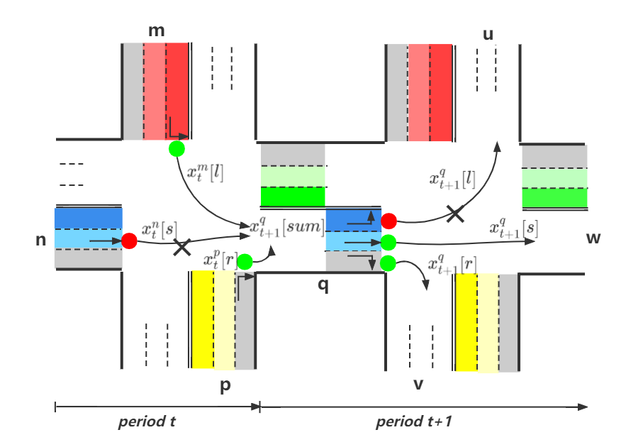
Figure 4. The transition of traffic flows for road $q$.

As we will show in the next section, Eq. (6) is actually supported by the fundamental transition equations from transportation.

Transition equations from transportation. From the perspective of transportation (Aboudolas et al., 2009; Varaiya, 2013), the traffic flow on a road segment consists of incoming and outgoing flow. In Figure 4, the traffic flows on road segment $q$ can be formulated as:

(7) $$\small\mathbf{x}_{t+1}^{q}[sum]=\mathbf{x}_{t}^{q}[sum]-\mathbf{x}_{t}^{q}[out]+\mathbf{x}_{t+1}^{q}[in]\\$$

where $\mathbf{x}_{t+1}^{q}[sum]$ denotes the total volume of traffic flow on road segment $q$ at time $t+1$, $\mathbf{x}_{t}^{q}[out]$ denotes the traffic volume leaving road segment $q$ at time $t$, and $\mathbf{x}_{t+1}^{q}[in]$ denotes the traffic volume that will arrive $q$ at time $t+1$.

Since the traffic flow is directional with downstream traffic flow coming from its upstream, which can be formulated as:

(8) $$\small\mathbf{x}_{t}^{q}[out]=\mathcal{A}_{t}^{q,u}\cdot\gamma^{q,u}\cdot\mathbf{x}_{t}^{q}[l]+\mathcal{A}_{t}^{q,w}\cdot\gamma^{q,w}\cdot\mathbf{x}_{t}^{q}[s]+\mathcal{A}_{t}^{q,v}\cdot\gamma^{q,v}\cdot\mathbf{x}_{t}^{q}[r]\\$$

(9) $$\small\mathbf{x}_{t+1}^{q}[in]=\mathcal{A}_{t}^{m,q}\cdot\gamma^{m,q}\cdot\mathbf{x}_{t}^{m}[l]+\mathcal{A}_{t}^{p,q}\cdot\gamma^{p,q}\cdot\mathbf{x}_{t}^{p}[r]+\mathcal{A}_{t}^{n,q}\cdot\gamma^{n,q}\cdot\mathbf{x}_{t}^{n}[s]\\$$

where $u$, $v$, $w$ denote the downstream road segments of $q$, $\mathcal{A}_{t}^{i,j}$ denotes the connectivity of road segment $i$ and $j$ based on the Phase-activated Adjacency Matrix at time $t$, $\mathcal{A}_{t}^{i,j}=1$ if road segment $i$ and $j$ is connected. $\gamma^{i,j}$ is the saturation flow rate in transportation (Varaiya, 2013; Hurdle, 1984), which is a physical constant for $i$ and $j$, indicating the proportion of traffic volume that flows from $i$ to downstream $j$.

Intuitively, Eq. (8) indicates the outgoing flows are directional, moving from $q$ to its downstream roads that are permitted by traffic signals. Similarly, Eq. (9) indicates the incoming flows are also directional, moving from $q$’s upstream roads to $q$ are permitted by traffic signals. Specifically, as the proportion of traffic volume from $i$ to $j$, $\gamma^{i,j}$ considers the real-world situations where not all the intended traffic from $i$ to $j$ could be satisfied, due to physical road designs like speed limit, number of lanes, etc. (Hurdle, 1984).

Theorem 4.1 (Connection with transition equations).

The latent traffic volume calculated by Eq. (6) equals to the transition equations, Eq. (8) and Eq. (9) from transportation.

Proof.

The proof can be done by expanding out the calculation for every element in $\textbf{Z}_{t}$.

For any $\tau\in\{1,\dots,T\}$, the latent traffic state $\widehat{\textbf{Z}}_{t-\tau+1}^{i}$ on road segment $i$ at time $t-\tau+1$ can be inferred by aggregating the features of all upstream traffic flows (allowed by traffic signal phase), which is similar to transition equations, Eq. (8) and Eq. (9).

(10) $$\widehat{\textbf{Z}}_{t-\tau+1}^{i} =\sum_{j\in\mathcal{N}_{t-\tau}(i)}\mathcal{A}_{t-\tau}^{j,i}\cdot\gamma^{j,i}\cdot\textbf{X}_{t-\tau}^{j}$$

$$=\sum_{j\in\mathcal{N}_{t-\tau}(i)}(\mathcal{A}_{t-\tau}\odot\gamma)^{j,i}\cdot\textbf{X}_{t-\tau}^{j}$$

where $\mathcal{N}_{t}(i)$ denotes upstreams of road segment $i$. When we set $\gamma^{j,i}\in\textbf{Att}^{\intercal}$, the above equation equals to Eq. (6). Similar deduction also applys for Eq. (9).

∎

The transition equations  (8) and (9) could be considered as the propagation and aggregation process of $\textbf{X}_{t}$ toward $\widehat{\textbf{Z}}_{t+1}$ under the guidance of Phase-activated Adjacency Matrix $\mathcal{A}_{t}$, and the attention matrix Att modeled by the base GNN module. According to Eq. (7), a combination between $\textbf{X}_{t}$ and $\widehat{\textbf{Z}}_{t+1}$ could be applied for the final prediction for $\textbf{X}_{t+1}$ to combine Eq. (8) and Eq. (9).

4.3.3. Output Layer

After Neural Transition Layer, an output layer is designed to model the combinations indicated by Eq. (7). The output layer contains residual connections to comply with Eq. (7) and alleviate the over-smoothing problem. A fully connected layer is also applied to make sure the output of the network and the forecasting target have the same dimension. The final output is:

(11) $$\small\widehat{\textbf{X}}_{t+1}=ReLU(\sigma(\widehat{\textbf{Z}}_{t+1}+\textbf{X}_{t})\textbf{W}_{L}+\textbf{b}_{L})$$

where $\textbf{W}_{L}$ and $\textbf{b}_{L}$ are learnable weights.

4.4. Iterative Imputation for Prediction

Our model takes $T$ slices of X as input, and output two types of values: the prediction traffic volume of road segments in the historical $T-1$ time steps $(\widehat{\textbf{X}}_{t-T+2},\widehat{\textbf{X}}_{t-T+3},\cdots,\widehat{\textbf{X}}_{t})$ and states of all road segments in the next time step $\widehat{\textbf{X}}_{t+1}$. At iteration $\tau$, the model would provide the predicted traffic volumes $\widehat{\textbf{X}}_{t-\tau}$ on all the road segments for time $t-\tau+1$ , no matter accurate or not. Then the unobserved part from predicted traffic volume $\widehat{\ddot{\textbf{X}}}_{t-\tau+1}$ will be merged with the observed states $\dot{\textbf{X}}_{t-\tau+1}$ as merged states ${\textbf{X}}^{\prime}_{t-\tau+1}$ for $t-\tau+1$:

(12) $$\footnotesize{\textbf{X}}^{\prime}_{t-\tau+1}=\dot{\textbf{X}}_{t-\tau+1}+\widehat{\ddot{\textbf{X}}}_{t-\tau+1}={\textbf{X}}_{t-\tau+1}\odot\textbf{M}+\widehat{\textbf{X}}_{t-\tau+1}\odot(1-\textbf{M})$$

Then ${\textbf{X}}^{\prime}_{t-\tau+1}$, along with the imputed states from previous iterations $\{{\textbf{X}}^{\prime}_{t-T+1},\cdots,{\textbf{X}}^{\prime}_{t-\tau}\}$ and observed states for future iterations $\{\dot{\textbf{X}}_{t-\tau+2},\cdots,\dot{\textbf{X}}_{t}\}$, would be used to predict ${\widehat{\textbf{X}}}_{t-\tau+2}$ for the next iteration. Since the first iteration do not have predictions from the past, random values are generated as $\widehat{\textbf{X}}_{t-T+1}$. At the last iteration, we will have all the past merged states (${\textbf{X}}^{\prime}_{t-T+1},{\textbf{X}}^{\prime}_{t-\tau+1},\cdots,{\textbf{X}}^{\prime}_{t}$), and the predicted value $\widehat{\textbf{X}}_{t+1}$ will be used as the final prediction.  
 Loss function. Our loss function is proposed as follows:

(13) $$\small\begin{split}\min\limits_{\theta}\mathcal{L}_{p}(\theta)=&\frac{1}{T-1}\frac{1}{N}\sum_{i=1}^{T-1}\sum_{j=1}^{N}\parallel(\textbf{x}^{j}_{T-i}-\widehat{\textbf{x}}^{j}_{T-i})\odot\textbf{M}^{j}\parallel_{2}\\[-3.87498pt] &+\frac{1}{N}\sum_{j=1}^{N}\parallel(\textbf{x}^{j}_{T+1}-\widehat{\textbf{x}}^{j}_{T+1})\odot\textbf{M}^{j}\parallel_{2}\\ \end{split}$$

where $\theta$ are the model parameters to update, $T$ is the historical time step, and N is the number of all the road segments in the network. The first part of Eq. (13) aims to minimize loss for imputation, and the second part aims to minimize loss for prediction. With the mask matrix M, our model is optimized over the observed tensor $\dot{\textbf{X}}_{j}$, but with iterative imputation, the prediction on unobserved states could also be optimized. The detailed algorithm can be found in Appendix A.

5. Experiments

In this section, we conduct experiments to answer the following research questions:

$\bullet$ RQ1: Compared with state-of-the-arts, how does DTIGNN perform?

$\bullet$ RQ2: How do different components affect DTIGNN?

$\bullet$ RQ3: Is DTIGNN flexible to be integrated into existing methods?

$\bullet$ RQ4: How does DTIGNN support downstream tasks?

Table 1. The MAE, RMSE and MAPE of different methods on synthetic data and real-world data. The lower, the better.

Datasets	Metrics	STGCN (Yu et al., 2017b)	STSGCN (Song et al., 2020)	ASTGCN(Guo et al., 2019)	ASTGNN(Guo et al., 2021)	WaveNet (Wu et al., 2019)	Ours (ASTGNN)	Ours (WaveNet)
$D_{4\times 4}$	MAE	0.0563	0.1244	0.0605	0.0562	0.0427	0.0484	0.0378
	RMSE	0.1885	0.2993	0.2092	0.2124	0.1981	0.1920	0.1825
	MAPE	0.0216	0.0460	0.0302	0.0256	0.0165	0.0215	0.0145
$D_{HZ}$	MAE	0.4909	0.6079	0.4458	0.4020	0.4556	0.3810	0.4071
	RMSE	0.8756	0.9104	0.7425	0.7408	0.8668	0.6618	0.6883
	MAPE	0.3135	0.3863	0.2953	0.2527	0.2987	0.2455	0.2599
$D_{NY}$	MAE	0.2651	0.4476	0.3136	0.2437	0.2168	0.2437	0.2306
	RMSE	1.1544	1.1235	1.0625	1.0704	1.1485	0.9493	1.1002
	MAPE	0.1146	0.2358	0.1620	0.1272	0.0988	0.1283	0.1207

5.1. Datasets

We verify the performance of DTIGNN on a synthetic traffic dataset $D_{4\times 4}$ and two real-world datasets, $D_{HZ}$ and $D_{NY}$, where the road-segment level traffic volume are recorded with traffic signal phases. We generate sparse data by randomly masking several intersections out to mimic the real-world situation where the roadside surveillance cameras are not installed at certain intersections. Detailed descriptions and statistics can be found in Appendix B.  
 $\bullet$ $D_{4\times 4}$. The synthetic dataset is generated by the open-source microscopic traffic simulator CityFlow (Zhang et al., 2019). The traffic simulator takes $4\times 4$ grid road network and the traffic demand data as input, and simulates vehicles movements and traffic signal phases. The dataset is collected by logging the traffic states and signal phases provided by the simulator at every 10 seconds and randomly masking out several intersections.  
 $\bullet$ $D_{HZ}$. This is a public traffic dataset that covers a $4\times 4$ network in Hangzhou, collected from surveillance cameras near intersections in 2016. This dataset records the position and speed of every vehicle at every second. Then we aggregate the real-world observations into 10-second intervals on road-segment level traffic volume, which means there are 360 time steps in the traffic flow for one hour. We treat these records as groundtruth observations and sample observed traffic states by randomly masking out several intersections.  
 $\bullet$  $D_{NY}$. This is a public traffic dataset that covers a $7\times 28$ network in New York, collected by both camera data and taxi trajectory data in 2016. We sampled the observations in a similar way as in $D_{HZ}$.

5.2. Baseline Methods

We compare our model mainly on data-driven baseline methods. For fair comparison, unless specified, all the methods are using the same data input, including the observed traffic volumes and traffic signal information.  
 $\bullet$ Spatio-Temporal Graph Convolution Network (STGCN) (Yu et al., 2017b): STGCN is a data-driven model that utilizes graph convolution and 1D convolution to capture spatial and temporal dependencies respectively.  
 $\bullet$ Spatial-Temporal Synchronous Graph Convolutional Networks (STSGCN) (Song et al., 2020): STSGCN utilizes multiple localized spatial-temporal subgraph modules to capture the localized spatial-temporal correlations directly.  
 $\bullet$ Attention based Spatial Temporal Graph Convolutional Networks (ASTGCN) (Guo et al., 2019): ASTGCN uses spatial and temporal attention mechanisms to model spatial-temporal dynamics.  
 $\bullet$ Attention based Spatial Temporal Graph Neural Networks (ASTGNN) (Guo et al., 2021): Based on ASTGCN, ASTGNN further uses a dynamic graph convolution module to capture dynamic spatial correlations.  
 $\bullet$ GraphWaveNet (WaveNet) (Wu et al., 2019): WaveNet combines adaptive graph convolution with dilated casual convolution to capture spatial-temporal dependencies.

5.3. Experimental Settings and Metrics

Here we introduce some of the important experimental settings and detailed hyperparameter settings can be found in Appendix C. We split all datasets with a ratio 6: 2: 2 into training, validation, and test sets. We generate sequence samples by sliding a window of width $T+T^{\prime}$. Specifically, each sample sequence consists of 31 time steps, where 30 time steps are treated as the input while the last one is regarded as the groundtruth for prediction.

Following existing studies (Guo et al., 2019, 2021; Li et al., 2017; Song et al., 2020; Yao et al., 2019), MAE, RMSE and MAPE are adopted to measure the errors between predicted against groundtruth traffic volume. Their detailed formula for calculation can be found in Appendix D.

5.4. Overall Performance (RQ1)

In this section, we investigate the performance of DTIGNN on predicting the next traffic states under both synthetic data and real-world data. Table 1 shows the performance of DTIGNN, traditional transportation models and state-of-the-art data-driven methods. We have the following observations:  
 $\bullet$ Among the data-driven baseline models, WaveNet and ASTGNN perform relatively better than other baseline methods in $D_{4\times 4}$ and $D_{NY}$. One reason is that these two models have a special design to capture the dynamic spatial graph, which could explicitly model the dynamic connectivity between road segments.  
 $\bullet$ DTIGNN can achieve consistent performance improvements over state-of-the-art prediction methods, including the best baseline models like Wavenet and ASTGNN. This is because DTIGNN not only models the dynamic connectivity explicitly with the dynamic adjacency matrix, but also incorporates transition equations and imputation in the training process, the influences of missing observations are further mitigated. As we will see in Section 5.5.3, our proposed method can be easily integrated into the existing baseline methods and achieve consistent improvements.

5.5. Model Analysis

To get deeper insights into DTIGNN, we also investigate the following aspects about our model with empirical results: (1) ablation study on different parts of proposed components, (2) the effectiveness of imputation with prediction in one model, and (3) the sensitivity of DTIGNN on different base models and under different data sparsity.

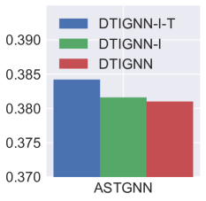
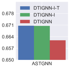
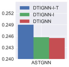
(a) MAE	(b) RMSE	(c) MAPE

Figure 5. MAE, RSME and MAPE of DTIGNN with the influence of different components on $D_{HZ}$. The lower, the better.

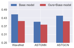
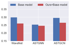
(a) MAE	(b) RMSE	(c) MAPE

Figure 6. MAE, RSME and MAPE of the variants of DTIGNN against different baseline models on $D_{HZ}$. The lower, the better. The variants of DTIGNN are implemented on corresponding baseline models. DTIGNN achieves the better performance over corresponding baseline models. Similar trends are also found on other datasets.

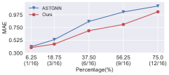
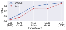
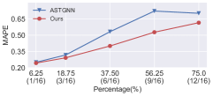
(a) MAE	(b) RMSE	(c) MAPE

Figure 7. MAE, RSME and MAPE of DTIGNN against baseline models under different levels of sparsity on $D_{HZ}$. The lower, the better. The x-axis indicates the percentage of sparsity, which is calculated with the number of unobserved intersections divided by total number of intersections in the network (here $D_{HZ}$ has 16 intersections) in percentage. Our proposed model achieves consistent better performance under different sparsity.

5.5.1. Ablation Study (RQ2)

In this section, we perform an ablation study to measure the importance of dynamic graph and imputation on the following variants:  
 $\bullet$ DTIGNN-I-T. This model takes both the network-level traffic volume and signal phases as its input and outputs the future traffic volume directly, which does not include Neural Transition Layer to model the transition equations and does not have imputation in the training process. It can also be seen as the baseline model ASTGNN with additional node features of traffic signal phases.  
 $\bullet$ DTIGNN-I. Based on DTIGNN-I-T, this model additionally uses Neural Transition Layer to incorporate transition equations, while it does not impute the sparse data in the training process.  
 $\bullet$ DTIGNN. This is our final model, which integrates Neural Transition Layer, and imputes sparse observations in the training process.

Figure 5 shows the performance of the variants. We can observe that DTIGNN-I outperforms DTIGNN-I-T, indicating the effectiveness of Neural Transition Layer as a way to incorporate transition equations. DTIGNN further outperforms DTIGNN-I, since it iteratively imputes the sparse data in the training process and optimize the imputation and prediction at the same time.

Table 2. Performance of DTIGNN against different baselines and their corresponding two-step variants on $D_{HZ}$. The lower, the better. Vanilla baseline methods and DTIGNN learn from sparse observations, while the two-step variants impute sparse observations first and train on the imputed data. DTIGNN achieves the best performance in all cases. Similar trends are also found on other datasets.

Method	MSE	RMSE	MAPE
ASTGCN (vanilla)	0.4458	0.7425	0.2953
ASTGCN (two step)	0.4423	0.7417	0.2928
WaveNet (vanilla)	0.4556	0.8668	0.2987
WaveNet (two step)	0.4104	0.6977	0.2594
ASTGNN (vanilla)	0.4020	0.7408	0.2527
ASTGNN (two step)	0.3842	0.6706	0.2490
Ours	0.3810	0.6618	0.2455

5.5.2. Imputation Study

To better understand how imputation helps prediction, we compare two representative baselines with their two-step variants. Firstly, we use a pre-trained imputation model to impute the sparse data following the idea of (Tang et al., 2019; Yi et al., 2019). Then we train the baselines on the imputed data.

Table 2 shows the performance of baseline methods in $D_{HZ}$. We find out that the vanilla baseline methods without any imputation show inferior performance than the two-step approaches, which indicates the importance of imputation in dealing with missing states. DTIGNN further outperforms the two-step approaches. This is because DTIGNN learns imputation and prediction in one step, combining the imputation and prediction iteratively across the whole framework. Similar results can also be found in$D_{4\times 4}$ and $D_{NY}$, and we omit these results due to page limits.

5.5.3. Sensitivity Study

In this section, we evaluate the sensitivity of DTIGNN with different base models and different data sparsity.  
 $\bullet$ Choice of base model. (RQ3) DTIGNN can be easily integrated with different GNN structures. To better understand how different base models influence the final performance, we compare DTIGNN with different GNN models as base GNN modules against corresponding GNN models. Figure 6 summarizes the experimental results. Our proposed method performs steadily under different base models across various metrics, indicating the idea of our method is valid across different base models. In the rest of our experiments, we use ASTGNN as our base model and compare it with other methods.  
 $\bullet$  Data sparsity. In this section, we investigate how different sampling strategies influence DTIGNN. We randomly sample 1, 3, 6, 9, 12 intersections out of 16 intersections from $D_{HZ}$ and treat them unobserved to get different sampling rates. We set the road segments around the sampled intersections as the missing segments and evaluate the performance of our model in predicting the traffic volumes for all the road segments. As is shown in Figure 7, with sparser observations, DTIGNN performs better than ASTGNN with lower errors, though the errors of both methods increase. Even when over half the observations are missing, our proposed method can still predict future traffic states with lower errors, indicating the consistency of DTIGNN under a wide range of sparsity.

5.6. Case Study (RQ4)

To test the feasibility of using our proposed model in the downstream tasks, we conduct experiments on a traffic signal control task, where only part of traffic states in the road network is observable. Ideally, adaptive signal control models take the full states as input and provide actions to the environment, which then executes the traffic signal actions from the control models. However, in the sparse data setting, the signal models at unobserved intersections will fail to generate any adaptive actions since there is no state as input. With a well-trained state transition model, the full traffic states could be predicted for all the intersections, upon which the signal control models could generate actions. Intuitively, a good state transition model would provide the signal controller with more precise states, and enable better results in traffic signal control.

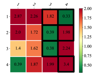
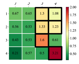
(a) RMSE of baseline (left) and DTIGNN (right). The lower, the better.
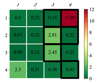
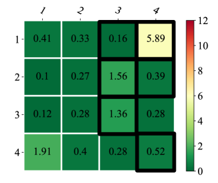
(b) Queue length of MaxPressure using predictions from baseline (left) and DTIGNN (right). The lower, the better.

Figure 8. The performance of the baseline method and DTIGNN under sparse data on $D_{HZ}$ for two sequential tasks: traffic state modeling w.r.t. RMSE, and traffic signal control w.r.t. queue length using MaxPressure. The x-axis and y-axis indicate the location of the intersections in the road network of $D_{HZ}$. The black boxes indicate the intersections without any observation. DTIGNN has lower prediction error in predicting next traffic states. These predictions are then used by MaxPressure (Varaiya, 2013) to achieve better performance with a lower average queue length. Best viewed in color.

The experiment is conducted on the traffic simulator CityFlow (Zhang et al., 2019) with $D_{HZ}$. We use the states returned by the traffic simulator as full states and mask out the observations of several intersections to mimic the sparse data setting. Based on the sparse data, state transition models can predict the full future states. Then the traffic signal control model (here we use an adaptive model, MaxPressure (Varaiya, 2013)) will decide the actions and feed the actions into the simulator. We compare the performance of DTIGNN against ASTGNN, the best baseline model on $D_{HZ}$, for the state transition task and the traffic signal control task. For traffic signal control task, the average queue length of each intersection and the average travel time of all the vehicles are used as metrics, following the existing studies (Wei et al., 2018; Zhang et al., 2019). Detailed descriptions can be found in Appendix E.

Figure 8 shows the experimental results for each intersection in $D_{HZ}$, and we have the following observations:  
 $\bullet$ DTIGNN has better performance in both predicting traffic states and traffic signal control in Figure 8(a) and Figure 8(b). We also measure the average travel time of all vehicles in the network and found out that the average travel time by DTIGNN is 494.26 seconds, compared to the 670.45 seconds by ASTGNN. This indicates that DTIGNN can better alleviate downstream signal control task that suffers from missing data problems.  
 $\bullet$ We also notice that, although ASTGNN shows lower RMSE on certain intersections (e.g., intersection 1_4, 2_3, 3_3 on the left of Figure 8(a)), its performance on traffic signal control result is inferior. This is because network-level traffic signal control requires observation and coordination between neighboring intersections, which requires accurate modeling on global traffic states. In contrast, DTIGNN shows satisfactory prediction performance on the global states and thus achieve better performance on traffic signal control task even when the traffic signal controller.

6. Conclusion

In this paper, we propose a novel and flexible approach to model the network-level traffic flow transition. Specifically, our model learns on the dynamic graph induced by traffic signals with a network design grounded by transition equations from transportation, and predicts future traffic states with imputation in the process. We conduct extensive experiments using synthetic and real-world data and demonstrate the superior performance of our proposed method over state-of-the-art methods. We further show in-depth case studies to understand how the state transition models help downstream tasks like traffic signal control, even for intersections without any traffic flow observations.

We would like to point out several important future directions to make the method more applicable to the real world. First, more traffic operations can be considered in the modeling of transitions, including road closures and reversible lanes. Second, the raw data for observation only include the phase and the number of vehicles on each lane. More exterior data like the road and weather conditions might help to boost model performance.

Appendix A algorithm

Input: Observed state tensor $\dot{\mathcal{X}}=(\dot{X}_{t-T+1},\dot{X}_{t-T+2},\cdots,\dot{X}_{t})$, phase Activate Matrix $(\mathcal{A}_{t-T+1},\mathcal{A}_{t-T+2},\cdots,\mathcal{A}_{t})$, Static Adjacency Matrix $\mathcal{A}$, initial training options and model’s parameters $\theta_{0}$, etc.

Output: $X=(X_{t+1})$, the last dimension is 3 dimensions represent l,s,r traffic volumes of road segments,respectively.

for $epoch\leftarrow{0,1,\cdots}$ do

       for $\tau\leftarrow{t-T+1,\cdots,t}$ do

             // Base GNN Module

             Generate Attentation Matrix $Att$ using Eq (4);

             // Neural Transition Layer

             Generate Proportion Matrix $\Gamma_{t}$;

             Calculate latent states $\widehat{\textbf{Z}}_{\tau}$ using Eq (6);

             // Output Layer

             Predict traffic states of unobserved road segments using Eq (11) ;

             Impute on $\ddot{\textbf{X}}_{\tau}$ with Eq (12)

       end for

      Predict $X$;

       Update $\theta$ by minimize the training loss with Eq (13)

end for

Algorithm 1 Training procedure of DTIGNN

Appendix B Dataset Description

We conduct experiments on one synthetic traffic dataset $D_{4\times 4}$ and two real-world datasets, $D_{HZ}$ and $D_{NY}$, where the road-segment level traffic volume are recorded with traffic signal phases. The data statistics are shown in Table 3, and the road networks in these datasets are shown in Figure 9 and Figure 10.

Table 3. Statistics of datasets.

Dataset	$D_{4\times 4}$	$D_{HZ}$	$D_{NY}$
Duration (seconds)	3600	3600	3600
Time steps	360	360	360
# of intersections	16	16	196
# of road segments	80	80	854
# of groundtruth states (full)	23040	23040	282240
% of unobserved intersections	12.5	12.5	10.4

$\bullet$ $D_{4\times 4}$. The synthetic dataset is generated by the open-source microscopic traffic simulator CityFlow (Zhang et al., 2019). The traffic simulator takes $4\times 4$ grid road network and the traffic demand data (represented as the origin and destination location, the route and the start time) as input, and simulates vehicles movements and traffic signal phases. Each intersection in the road network has four directions (West$\rightarrow$East, East$\rightarrow$West, South$\rightarrow$North, and North$\rightarrow$South), and 3 lanes (300 meters in length and 3 meters in width) for each direction. Vehicles come uniformly with 180 vehicles/lane/hour in both West$\leftrightarrow$East direction and South$\leftrightarrow$North direction. The dataset is collected by logging the traffic states and signal phases provided by the simulator at every 10 seconds and randomly masking out several intersections.  
 $\bullet$ $D_{HZ}$. This is a public traffic dataset that covers a $4\times 4$ network of Gudang area in Hangzhou, collected from surveillance cameras near intersections in 2016. This dataset records the position and speed of every vehicle at every 1 second. Then we aggregate the real-world observations into 10-second intervals on road-segment level traffic volume, which means there are 360 time steps in the traffic flow for one hour. We treat these records as groundtruth observations trajectories and sample observed traffic states by randomly masking out several intersections.  
 $\bullet$  $D_{NY}$. This is a public traffic that dataset covers a $7\times 28$ network of Upper East Side of Manhattan, New York, collected by both camera data and taxi trajectory data in 2016. This dataset records the lane-level volumes at every 10 second, which means there are 360 time steps in the traffic flow for one hour. We sampled the sparse observations in a similar way as in $D_{HZ}$.

Appendix C Hyperparameter Settings

Some of the important hyperparameters can be found in Table 4.

Table 4. Hyper-parameter settings for DTIGNN.

Parameter	Value	Parameter	Value
Batch size	32	Historical time slice $T$	30
Convolution kernel	64	Predict time slice $T^{\prime}$	1
Time interval of raw data	10(s)	Input channel	11
Chebyshev polynomial	3	Output channel	3
Learning rate	0.001	Training epochs	100

Appendix D Evaluation Metrics

We use MAE, RMSE and MAPE to evaluate the performance of predicting next state, which are defined as:

(14) $$MAE=\frac{1}{N}\frac{1}{F}\mathop{\sum}_{i=1}^{N}\mathop{\sum}_{j=1}^{F}|\textbf{x}_{t}^{i,j}-\hat{\textbf{x}}^{i,j}_{t}|$$

(15) $$RMSE=\sqrt{\frac{1}{N}\frac{1}{F}\mathop{\sum}_{i=1}^{N}\mathop{\sum}_{j=1}^{F}||\textbf{x}_{t}^{i,j}-\hat{\textbf{x}}^{i,j}_{t}||^{2}}$$

(16) $$MAPE=\begin{cases}&\frac{1}{N}\frac{1}{F}\mathop{\sum}_{i=1}^{N}\mathop{\sum}_{j=1}^{F}\frac{|\textbf{x}_{t}^{i,j}-\hat{\textbf{x}}^{i,j}_{t}|}{\textbf{x}_{t}^{i,j}},\ \textbf{x}_{t}^{i,j}\not=0\\ &1,\ \textbf{x}_{t}^{i,j}=0,\&\textbf{x}_{t}^{i,j}\not=\hat{\textbf{x}}^{i,j}_{t}\\ &0,\ \textbf{x}_{t}^{i,j}=0,\&\textbf{x}_{t}^{i,j}=\hat{\textbf{x}}^{i,j}_{t}\\ \end{cases}$$

where $N$ is the total number of road segments, $F$ is the size of observed state vector on the road segment, $\textbf{x}_{t}^{i,j}$ and $\hat{\textbf{x}}^{i,j}_{t}$ are the $j$-th element in the traffic volume states of $i$-th road segment at time $t$ in the ground truth and predicted traffic volumes relatively.

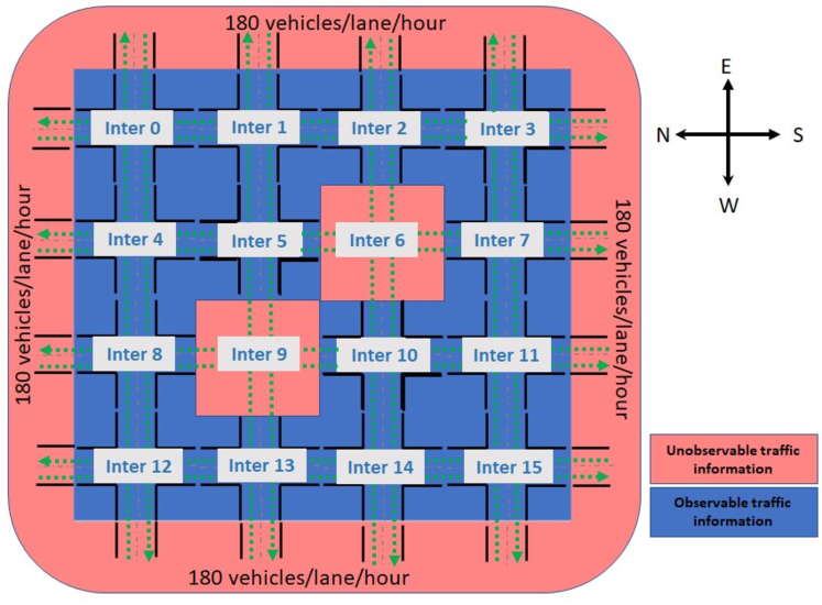
Figure 9. Road networks for synthetic data set. $D_{4\times 4}$ has 16 intersections with bi-directional traffic. Green dot lines represent traffic flow direction on each lane. Traffic information in the red regions is unobservable while in the blue region information is entirely recorded.

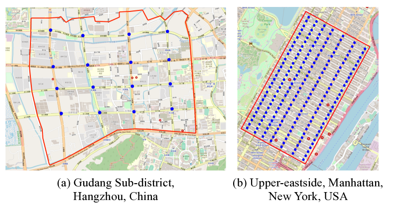
Figure 10. Road networks for real-world datasets. Red polygons are the areas we select to model, blue dots are intersections with traffic signals. (a) $D_{HZ}$, 16 intersections with uni- & bi-directional traffic. (b) $D_{NY}$, 196 intersections with uni-directional traffic.

Appendix E Case Study Settings

The traffic signal control task requires the simulator to provide the groundtruth states. After having the states, we mask out the states for several intersections and provide sparse state observations to the traffic signal models. Ideally, the signal control models would take the full states as input and provide actions to the simulator, which would then executes the traffic signal actions from the control method. However, in the sparse data setting, the traffic signal controller at unobserved intersections will not be able to generate any actions since it has no state as input. With a well-trained state transition model, the full traffic states could be predicted all the intersections, upon which the signal control models would be able to generate actions.

Following the settings in traffic signal methods (Wei et al., 2018, 2019),we process the traffic dataset into a format acceptable by the simulator CityFlow (Zhang et al., 2019). In the processed traffic dataset for the simultor, each vehicle is described as $(o,t,d)$, where $o$ is the origin location, $t$ is time, and $d$ is the destination location. Locations $o$ and $d$ are both locations on the road network. Each green signal is followed by a three-second yellow signal and two-second all red time.

At each time step, we acquire the full state observations from the simulator, mask traffic observations in part of intersections as missing data, and use the state transition model to predict these the next states for all the road segments. Then baseline model ASTGNN and DTIGNN are used as the transition model to recover missing values returned from the simulator and exploit the recovered observations. MaxPressure controller then decides the next traffic signal phase and feed the actions into the simulator. During this process, we can collect groundtruth traffic states from the simulator environment, and predict values from our transition model. After one round of simulation (here we set as 3600 seconds with action interval as 10 seconds), we get the average travel time from the environment and the average queue length for each intersection to evaluate the performance for traffic signal control task.

Appendix F Exploration about Loss Function

We attempt to incorporate graph contrastive learning (Zhu et al., 2020) into the model to make the model learn additional representations from the prediction. The goal of graph contrastive learning is to learn an embedding space in which positive pairs stay close to each other while negative ones are far apart. In the case of this paper, positive pairs are defined as outputs generated by model using the same input, while negative samples are defined as outputs generated by model using different inputs. In the training process, we first generate two correlated graph views by randomly performing corruption on the model’s output. Then, we use the new loss function to not only minimize prediction loss but also maximize the agreement between outputs in these two views. We select loss function proposed by  (Zhu et al., 2020) and combine it with Eq. (13) to construct new loss function. In addition, Two loss functions, which combine loss function proposed by  (Zhu et al., 2020) and its variants separately, are proposed to better adapt to the scenario of traffic networks.  
 $\bullet$ $\mathcal{L}_{N}$. For any observable node $i$, its two outputs generated by model at time $T+1$, $u_{T+1}^{i}$ and $v_{T+1}^{i}$, form the positive sample, and outputs of nodes other than $i$ in the two views are regarded as negative samples. Formally, we define the critic $d(u,v)=s(f(u),f(v))$, where $s$ is the cosine similarity and $f$ is the output of model. The pairwise objective for each positive pair ($u_{T+1}^{i},v_{T+1}^{i}$) is defined as:

(17) $$\begin{split}\ell(u_{T+1}^{i},v_{T+1}^{i})=\log\frac{e^{d(u_{T+1}^{i},v_{T+1}^{i})/\tau}}{e^{d(u_{T+1}^{i},v_{T+1}^{i})/\tau}+\sum_{k=1}^{N}\mathbbm{1}_{[k\neq i]}e^{d(u_{T+1}^{i},v_{T+1}^{i})/\tau}}\end{split}$$

Where $\mathbbm{1}_{k\neq i}\in\{0,1\}$ is an indication that equals to 1 if $k\neq i$, and $\tau$ is a temperature parameter. Since two views are symmetric, the loss at $T+1$ for another view is defined similarly for $\ell(v_{T+1}^{i},u_{T+1}^{i})$. The definition of $\mathcal{L}_{N}$ is as follows:

(18) $$\begin{split}\mathcal{L}_{N}=\mathcal{L}_{p}+\frac{1}{2N}\sum_{i=1}^{N}[\ell(u_{T+1}^{i},v_{T+1}^{i})+\ell(v_{T+1}^{i},u_{T+1}^{i})]\end{split}$$

Where $\mathcal{L}_{p}$ represent loss function of Eq. (13). The goal of the remainder of $\mathcal{L}_{N}$ is to minimize the distance between pairs of positive samples and maximize the distance between pairs of negative samples.  
 $\bullet$ $\mathcal{L}_{N-N}$. Based on $\mathcal{L}_{N}$, $\mathcal{L}_{N-N}$ removes denominator of Eq. (17). It can be considered that we only need to make the positive pairs as close as possible regardless of the distance between the negative pairs. It is reasonable in traffic networks, for road segments that are considered main roads may have similar traffic flow values at the same time interval. The definition of $\mathcal{L}_{N-N}$ is as follows:

(19) $$\begin{split}\mathcal{L}_{N-N}=\mathcal{L}_{p}+\frac{1}{2N}\sum_{i=1}^{N}[\ell^{-}(u_{T+1}^{i},v_{T+1}^{i})+\ell^{-}(v_{T+1}^{i},u_{T+1}^{i})]\end{split}$$

Where $\ell^{-}(u_{T+1}^{i},v_{T+1}^{i})=d(u_{T+1}^{i},v_{T+1}^{i})/\tau$.

Table 5 shows the performance of the loss function and its variants. We can observe that DTIGNN with $\mathcal{L}_{N-N}$ outperforms DTIGNN with $\mathcal{L}_{N}$, indicating that there is no obvious negative pairs relationship between outputs produced by different inputs under the traffic scenario. Moreover, DTIGNN further outperforms DTIGNN with $\mathcal{L}_{N-N}$. We believe that the model’s method of constructing positive pairs may be too arbitrary to learn additional information, resulting in suboptimal performance.

Table 5. Performance of DTIGNN using different loss functions on $D_{HZ}$. The lower, the better. Similar trends are also found on other datasets.

Method	MSE	RMSE	MAPE
DTIGNN with $\mathcal{L}_{N}$	0.4588	0.8359	0.2969
DTIGNN with $\mathcal{L}_{N-N}$	0.4355	0.7282	0.2876
Ours	0.3810	0.6618	0.2455

References

- (1)
- Aboudolas et al. (2009) Konstantinos Aboudolas, Markos Papageorgiou, and Elias Kosmatopoulos. 2009. Store-and-forward based methods for the signal control problem in large-scale congested urban road networks. TR-C 17, 2 (2009).
- Batista et al. (2002) Gustavo EAPA Batista, Maria Carolina Monard, et al. 2002. A study of K-nearest neighbour as an imputation method. His 87, 251-260 (2002).
- Boel and Mihaylova (2006) René Boel and Lyudmila Mihaylova. 2006. A compositional stochastic model for real time freeway traffic simulation. TR-C (2006).
- Fang et al. (2021) Zheng Fang, Qingqing Long, Guojie Song, and Kunqing Xie. 2021. Spatial-temporal graph ode networks for traffic flow forecasting. In KDD’21. 364–373.
- Fu et al. (2020) Kun Fu, Fanlin Meng, Jieping Ye, and Zheng Wang. 2020. Compacteta: A fast inference system for travel time prediction. In KDD’20.
- García-Laencina et al. (2010) Pedro J García-Laencina, José-Luis Sancho-Gómez, et al. 2010. Pattern classification with missing data: a review. Neural Computing and Applications (2010).
- Guo et al. (2021) Shengnan Guo, Youfang Lin, et al. 2021. Learning Dynamics and Heterogeneity of Spatial-Temporal Graph Data for Traffic Forecasting. TKDE (2021).
- Guo et al. (2019) Shengnan Guo, Youfang Lin, Ning Feng, Chao Song, and Huaiyu Wan. 2019. Attention Based Spatial-Temporal Graph Convolutional Networks for Traffic Flow Forecasting. AAAI’19 (2019).
- Hurdle (1984) VF Hurdle. 1984. Signalized intersection delay models–a primer for the uninitiated. TR-B (1984).
- Jayarajah et al. (2018) Kasthuri Jayarajah, Andrew Tan, and Archan Misra. 2018. Understanding the interdependency of land use and mobility for urban planning. In UbiComp’18.
- Kim et al. (2020) Kihwan Kim, Seungmin Jin, et al. 2020. STGRAT: A Spatio-Temporal Graph Attention Network for Traffic Forecasting. CIKM’20 (2020).
- Koren et al. (2009) Yehuda Koren, Robert Bell, and Chris Volinsky. 2009. Matrix factorization techniques for recommender systems. Computer 42, 8 (2009).
- Kotsialos et al. (2002) Apostolos Kotsialos, Markos Papageorgiou, Christina Diakaki, Yannis Pavlis, and Frans Middelham. 2002. Traffic flow modeling of large-scale motorway networks using the macroscopic modeling tool METANET. TITS (2002).
- Li et al. (2019) Steven Cheng-Xian Li, Bo Jiang, et al. 2019. Misgan: Learning from incomplete data with generative adversarial networks. arXiv:1902.09599 (2019).
- Li et al. (2017) Yaguang Li, Rose Yu, et al. 2017. Diffusion convolutional recurrent neural network: Data-driven traffic forecasting. arXiv:1707.01926 (2017).
- Lin et al. (2018) Kaixiang Lin, Renyu Zhao, Zhe Xu, and Jiayu Zhou. 2018. Efficient large-scale fleet management via multi-agent deep reinforcement learning. In KDD’18.
- Liu et al. (2016) Qiang Liu, Shu Wu, Liang Wang, and Tieniu Tan. 2016. Predicting the next location: A recurrent model with spatial and temporal contexts. In AAAI’16.
- Luo et al. (2018) Yonghong Luo, Xiangrui Cai, Ying Zhang, Jun Xu, et al. 2018. Multivariate time series imputation with generative adversarial networks. In NeurIPS’18.
- Mazumder et al. (2010) Rahul Mazumder, Trevor Hastie, and Robert Tibshirani. 2010. Spectral regularization algorithms for learning large incomplete matrices. JMLR (2010).
- Oh et al. (2018) Simon Oh, Young-Ji Byon, Kitae Jang, and Hwasoo Yeo. 2018. Short-term travel-time prediction on highway: A review on model-based approach. KSCE Journal of Civil Engineering (2018).
- Qin et al. (2021) Huiling Qin, Xianyuan Zhan, Yuanxun Li, et al. 2021. Network-Wide Traffic States Imputation Using Self-interested Coalitional Learning. (2021).
- Song et al. (2020) Chao Song, Youfang Lin, Shengnan Guo, and Huaiyu Wan. 2020. Spatial-temporal synchronous graph convolutional networks: A new framework for spatial-temporal network data forecasting. In AAAI’20.
- Tang et al. (2019) Xianfeng Tang, Boqing Gong, Yanwei Yu, et al. 2019. Joint modeling of dense and incomplete trajectories for citywide traffic volume inference. In TheWebConf’19.
- Varaiya (2013) Pravin Varaiya. 2013. Max pressure control of a network of signalized intersections. Transportation Research Part C: Emerging Technologies 36 (2013), 177–195.
- Wang et al. (2019) Hongjian Wang, Xianfeng Tang, et al. 2019. A simple baseline for travel time estimation using large-scale trip data. TIST (2019).
- Wang et al. (2017) Jingyuan Wang, Chao Chen, et al. 2017. No longer sleeping with a bomb: a duet system for protecting urban safety from dangerous goods. In KDD’17.
- Wang et al. (2020) Xiaoyang Wang, Yao Ma, Yiqi Wang, Wei Jin, Xin Wang, et al. 2020. Traffic flow prediction via spatial temporal graph neural network. In TheWebConf’20.
- Wang et al. (2022) Yibing Wang, Mingming Zhao, et al. 2022. Real-time joint traffic state and model parameter estimation on freeways with fixed sensors and connected vehicles: State-of-the-art overview, methods, and case studies. TR-C (2022).
- Wei et al. (2019) Hua Wei, Chacha Chen, Guanjie Zheng, et al. 2019. Presslight: Learning max pressure control to coordinate traffic signals in arterial network. In KDD’19.
- Wei et al. (2018) Hua Wei, Guanjie Zheng, Huaxiu Yao, and Zhenhui Li. 2018. Intellilight: A reinforcement learning approach for intelligent traffic light control. In KDD’18.
- Wu et al. (2018) Cathy Wu, Alexandre M Bayen, and Ankur Mehta. 2018. Stabilizing traffic with autonomous vehicles. In ICRA’18. IEEE.
- Wu et al. (2019) Zonghan Wu, Shirui Pan, Guodong Long, et al. 2019. Graph wavenet for deep spatial-temporal graph modeling. arXiv:1906.00121 (2019).
- Wu et al. (2020) Zonghan Wu, Shirui Pan, Guodong Long, et al. 2020. Connecting the dots: Multivariate time series forecasting with graph neural networks. In CIKM’20.
- Yao et al. (2019) Huaxiu Yao, Xianfeng Tang, Hua Wei, et al. 2019. Revisiting spatial-temporal similarity: A deep learning framework for traffic prediction. In AAAI’19.
- Yao et al. (2018) Huaxiu Yao, Fei Wu, Jintao Ke, et al. 2018. Deep multi-view spatial-temporal network for taxi demand prediction. In AAAI.
- Yi et al. (2019) Xiuwen Yi, Zhewen Duan, Ting Li, et al. 2019. Citytraffic: Modeling citywide traffic via neural memorization and generalization approach. In CIKM’19.
- Yoon et al. (2018) Jinsung Yoon, James Jordon, and Mihaela Schaar. 2018. Gain: Missing data imputation using generative adversarial nets. In ICML’18.
- Yu et al. (2017b) Bing Yu, Haoteng Yin, and Zhanxing Zhu. 2017b. Spatio-temporal graph convolutional networks: A deep learning framework for traffic forecasting. arXiv:1709.04875 (2017).
- Yu et al. (2017a) Rose Yu, Yaguang Li, Cyrus Shahabi, Ugur Demiryurek, and Yan Liu. 2017a. Deep learning: A generic approach for extreme condition traffic forecasting. In SDM’17.
- Zhang et al. (2019) Huichu Zhang, Siyuan Feng, et al. 2019. Cityflow: A multi-agent reinforcement learning environment for large scale city traffic scenario. In TheWebConf’19.
- Zhang et al. (2017) Junbo Zhang, Yu Zheng, and Dekang Qi. 2017. Deep spatio-temporal residual networks for citywide crowd flows prediction. In AAAI’17.
- Zhang et al. (2020a) Xiyue Zhang, Chao Huang, et al. 2020a. Spatial-temporal convolutional graph attention networks for citywide traffic flow forecasting. In CKIM’18.
- Zhang et al. (2020b) Xiyue Zhang, Chao Huang, Yong Xu, et al. 2020b. Traffic Flow Forecasting with Spatial-Temporal Graph Diffusion Network. AAAI’20 (2020).
- Zhao et al. (2019) Ling Zhao, Yujiao Song, et al. 2019. T-gcn: A temporal graph convolutional network for traffic prediction. TITS’19 (2019).
- Zhu et al. (2020) Yanqiao Zhu, Yichen Xu, Feng Yu, Qiang Liu, Shu Wu, and Liang Wang. 2020. Deep graph contrastive representation learning. arXiv preprint arXiv:2006.04131 (2020).