Ji et al.

Risk-Aware Linear Bandit

Risk-Aware Linear Bandits: Theory and Applications in Smart Order Routing

Jingwei Ji Viterbi School of Engineering, University of Southern California, jingweij@usc.edu, Renyuan Xu Viterbi School of Engineering, University of Southern California, renyuanx@usc.edu, Ruihao Zhu SC Johnson College of Business, Cornell University, ruihao.zhu@cornell.edu

Motivated by practical considerations in machine learning for financial decision-making, such as risk aversion and large action space, we consider risk-aware bandits optimization with applications in smart order routing (SOR). Specifically, based on preliminary observations of linear price impacts made from the NASDAQ ITCH dataset, we initiate the study of risk-aware linear bandits. In this setting, we aim at minimizing regret, which measures our performance deficit compared to the optimum’s, under the mean-variance metric when facing a set of actions whose rewards are linear functions of (initially) unknown parameters. Driven by the variance-minimizing globally-optimal (G-optimal) design, we propose the novel instance-independent Risk-Aware Explore-then-Commit (RISE) algorithm and the instance-dependent Risk-Aware Successive Elimination (RISE++) algorithm. Then, we rigorously analyze their near-optimal regret upper bounds to show that, by leveraging the linear structure, our algorithms can dramatically reduce the regret when compared to existing methods. Finally, we demonstrate the performance of the algorithms by conducting extensive numerical experiments in the SOR setup using both synthetic datasets and the NASDAQ ITCH dataset. Our results reveal that 1) The linear structure assumption can indeed be well supported by the Nasdaq dataset; and more importantly 2) Both RISE and RISE++ can significantly outperform the competing methods, in terms of regret, especially in complex decision-making scenarios.

online learning, risk-aware bandits, regret analysis, smart order routing, algorithmic trading, mean-variance

1 Introduction

The increasing amount of financial data has revolutionized the techniques on data analytics, and brought new theoretical and computational challenges to the finance industry. In contrast to classic stochastic control theory and other analytical approaches, which typically reply heavily on model assumptions, machine learning based approaches can fully leverage the large amount of financial data. Moreover, they require much fewer model assumptions when utilized to improve financial decision-making (Hambly et al. 2021).

Among others, multi-armed bandit (MAB) is one of the most popular learning-based paradigms for sequential decision-making. At a high level, MAB concerns the scenario where an agent iteratively chooses one action/arm, among many, and then receives an action-specific random reward sampled from an (initially) unknown distribution. Rewards of other un-chosen actions remain unseen. The performance of the agent is (typically) measured by the notion of regret, which is the difference between the maximum expected total reward and the agent’s expected total reward. Here, the agent faces the classical exploration-exploitation dilemma, where she has to accurately learn the reward distribution of each action while collecting high rewards. Due to its flexibility and simplicity, MAB has found a wide variety of applications in revenue analytics (Li et al. 2010, Agrawal et al. 2019) and portfolio management (Shen et al. 2015).

In finance, a fundamental but largely overlooked problem of optimal executions across multiple venues, often referred to as smart order routing (SOR), could be naturally formulated into the MAB setup (see (Almgren and Chriss 2001, Cartea and Jaimungal 2016, Lin et al. 2015) for developments in the single-venue case). SOR is an automated trading procedure that seeks to find the best available way to execute orders among a range of different trading venues, including both lit pools and dark pools. A lit pool often refers to a public stock exchange where the order book is openly displayed and available for all participants. Dark pools are private exchanges only available to institutional investors. These private exchanges are known as “dark pools” due to their lack of transparency. When market participants have access to multiple venues and can split their orders and route the child orders to different venues for execution, the overall execution price and quantity could be improved significantly. Similar to the MAB setting, one of the key challenges of this problem is the partial observability and censored feedback of the orders submitted to dark pools (Agarwal et al. 2010). More specifically, only when an order is submitted to a given dark pool, can the market participant observes the corresponding executed amount (possibly smaller than the submitted order amount) and the execution price. This makes the MAB framework particularly suitable for modeling the SOR problem, as there is a natural exploration versus exploitation tradeoff.

Despite these, several challenges remain for the MAB to capture some main characteristics of the SOR problem and to be applied to a broader class of decision-making problems in finance:

• Challenge 1. Risk and Uncertainty: Most of the existing works in the MAB framework focus on maximizing the expected total reward for a risk-neutral agent. However, in many financial applications, reducing the risk and uncertainty of the outcome is equally important. In the SOR example, many institutional traders and brokers face the requirement of reducing the risk of their profits and losses (PnLs) or the worst-case losses made during a given period of time;

• Challenge 2. Large Action Space: For many financial decision-making problems, the action space can grow to prohibitively large, which prevents the direct adoption of the canonical MAB setup. Again in the SOR problem, for instance, splitting $V$ shares among $d$ venues results in $K=\Theta(V^{d})$ different actions This can easily make regret guarantee of many existing MAB algorithms vacuous.

To address Challenge 1, a recent line of works has started to develop learning algorithms that simultaneously achieve reward maximization and risk minimization. In these works, a commonly adopted measure that strikes the right balance between these two (potentially conflicting) goals is mean-variance (Markowitz 1952). Since its inception, the mean-variance metric has been widely adopted in many finance applications such as asset management and portfolio selection (Rubinstein 2002, Zhou and Yin 2003). In the mean-variance measure, the risk is quantified by the variance of the reward (i.e., deviation from the expected reward) and the objective is to minimize a difference between the total variance and the (weighted) expected total reward.

Regret minimization for MAB under the mean-variance measure is first considered by Sani et al. (2012) and then further studied in Vakili and Zhao (2016). Formally, let $T$ be the length of the entire time horizon of decision-making, and $X^{\pi}_{t}$ be the observed reward at time t. The cumulative mean-variance (MV) of policy $\pi$ is

$$\mathbb{E}\left[\sum_{t=1}^{T}\left(X_{t}^{\pi}-\frac{1}{T}\sum_{s=1}^{T}X_{s}^{\pi}\right)^{2}-\rho\sum_{t=1}^{T}X^{\pi}_{t}\right],$$ (1)

where $\rho\geq 0$ is the risk tolerance level. The regret is defined with respect to a policy which selects the best single action which attains the smallest MV. Compared with the canonical regret (without the variance term) considered in literature, the risk-aware regret is more amenable to financial applications, where the goal is not only to identify an optimal policy but also to ensure that the reward sequence collected remains stable throughout the learning process. This difference also arises some immediate difficulties. Under the measure of MV, regret can no longer be written as the sum of immediate performance loss at each time instant. Hence, a regret decomposition which involves higher-order statistics of the random time spent on each action is called upon.

However, as pointed out in Challenge 2, the number of actions $K$ can be prohibitively large in real-world applications. A direct application of methods from Sani et al. (2012), Vakili and Zhao (2016) may not yield a favorable performance guarantee, as the regret bounds can deteriorate rapidly with increasing $K$. To address this issue, many of the existing works propose to leverage the structure of the action space (see, e.g., part V of Lattimore and Szepesvári (2020) for a more thorough discussion). For example, a stream of works (Dani et al. 2008, Abbasi-Yadkori et al. 2011, Shipra Agrawal 2013) assumes that the expected reward of each action is an inner product between its feature vector and a common (initially) unknown parameter. This framework is known as the multiarmed bandit problem under a linear structure, or more succinctly as the linear bandit. Despite its name, this structure can integrate nonlinear information by constructing appropriate and possibly nonlinear feature/basis functions of our choice.

It turns out that in the SOR, our target application, the linear structure assumption aligns well with many empirical studies on price impacts observed in centralized limit order books(Bouchaud 2009). For instance, the practice of dividing large orders into smaller ones to minimize price impact is well-documented, with evidence indicating that the price impact of small orders is a polynomial of low degree relative to the order size (i.e., the action) (Bouchaud 2009, Cont et al. 2014). More specifically, as shown in Figure 1 using Amazon data, we observe a linear relationship between the average execution price and the order size (see Figure 1(a)) as well as another linear (up to noise perturbations) relationship between the variance of the execution price and the square of the order size (see Figure 1(b)). These evident relationships can be incorporated into a linear structure by introducing the order size and its square into the action vector (i.e., feature basis).

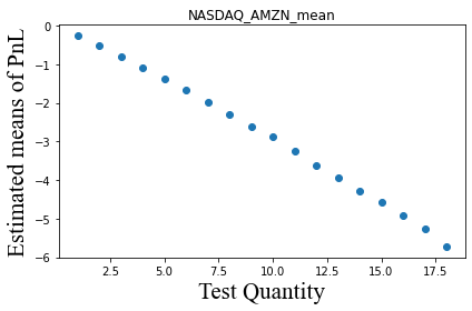
(a) AMZN NASDAQ mean with R-squared $R^{2}=0.99$

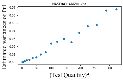
(b) AMZN NASDAQ var with R-squared $R^{2}=0.98$

Figure 1: The estimated means and variances of PnL for Amazon at NASDAQ exchange, at various test quantity to liquidate at each time point. This is an empirical justification for our linear form approximation.

Motivated by the above discussions, this paper focuses on regret minimization for bandits with a linear structure under the mean-variance metric, which appears to be the first of its kind to the best of our knowledge. In this case, the mean and variance of each action are assumed to have a linear structure on the action vector. Our main contributions can be summarized as follows:

• Modeling: We propose a modeling and learning framework designed to capture the key characteristics of many financial decision-making problems, notably a risk-sensitive objective and a large action space. To the best of our knowledge, this framework has not yet been investigated in the literature. In the context of SOR, as seen in Figure 1, we can introduce first, second, and even higher moments of the order size to capture the potentially nonlinear relationship between the reward and the action.

• Efficient Learning Algorithms: For the linear bandit setting, we propose two algorithms with near-optimal instance-independent regret upper bound and instance-dependent regret upper bound, respectively. Specifically, we first propose the Risk-Aware Explore-then-Commit (RISE) algorithm with instance-independent (i.e., worst case) regret upper bound of order $\tilde{O}(dT^{2/3}).$ To overcome the above-mentioned challenges, the algorithm follows the variance-minimizing G-optimal design (see, e.g., Chapter 21 of Lattimore and Szepesvári (2020)) to compute a distribution over a small subset of actions through which the unknown reward parameters can be learned efficiently. Then, RISE learns the unknown reward parameters by deploying this distribution. Afterwards, it sticks to a single action after a reasonable estimate of the unknown parameters is acquired.

  On the technical end, our analysis critically relies on a novel temporal decomposition of expected mean-variance regret (see Proposition 3.3). This is in sharp contrast to prior works, which would lead to polynomial dependence on the number of actions (which is typically large in our setting). This result helps to eliminate this dependence and dramatically reduce the mean-variance regret.

  To further exploit the possibly benign problem instances, we introduce the Risk-Aware Successive Elimination (RISE++) algorithm with instance-dependent bound of order $O(d^{3}\log(d)\log^{3}(KT))$. The algorithm runs in phases. In each phase, it explores the remaining actions using the re-computed G-optimal design (w.r.t. the remaining actions). Afterwards, it estimates the reward parameters with the collected data, and eliminates actions with poor estimated mean-variance values.

  While the instance-independent regret upper bound guarantees the growth rate of the expected regret (w.r.t. $T$) for all possible problem parameters, the instance-dependent regret upper bound can provide exponential improvement (w.r.t. $T$) for the growth rate of expected regret when the problem parameters are in our favor. We remark that both algorithms’ regret upper bounds successfully decouple the dependence on $K$ from that of $T$, which greatly reduce the regret when compared to existing approaches (see e.g., Sani et al. (2012), Vakili and Zhao (2016)), especially when the number of actions grows large. Hence, our algorithms are potentially more suitable for practical usage. When compared to the lower bounds developed in Vakili and Zhao (2016), both RISE and RISE++ enjoy nearly optimal (up to poly-logarithmic factors) dependence on $T$.

  Furthermore, driven by the practical necessity to adjust decisions according to evolving market conditions, we also study the extension of the contextual bandit (see Online Companion 9), wherein the coefficients are allowed to depend on the contexts. In this case, market information like order flow imbalance and volatilities can be integrated.

• Numerical Experiments for Smart Order Routing: To complement the above, we implement RISE and RISE++ on both synthetic datasets and the NASDAQ ITCH dataset for the SOR problem. Along the way, we first formally delineate the linear approximation of the SOR problem, with empirical evidence showing that the approximation error is small on the NASDAQ ITCH dataset. Then, we show that our proposed algorithms can significantly outperform competing methods in the literature for SOR in terms of regret.

• Comparisons with the Preliminary Version: A preliminary version of this paper ( 2022) has been published in Proceedings of the Third ACM International Conference on AI in Finance, in which only instance-independent regret upper bound (i.e., RISE) is established and the proposed algorithm is only tested on synthetic datasets. This version extends the preliminary version in several directions with substantial developments. In particular:

  1. We eliminate an additional additive factor of $O(d^{2})$ in the upper bound of RISE  by deriving a novel temporal decomposition of the regret.

  2. We further develop RISE++ that is capable of providing a near-optimal instance-dependent regret upper bound. It helps to capture the potentially more benign decision-making environment in our setting; and

  3. Motivated by practical need, we also propose a instance-independent bound for the contextual bandit setting. More importantly, we also provide a more thorough numerical experiment based on the NASDAQ ITCH dataset. This demonstrates the practicality of our proposed methods on real-world scenarios.

1.1 Related Literature

In this section, we discuss the existing results in literature and highlight the technical difficulty in our problem.

The linear bandit problem was first studied by Auer (2002) under the name of linear reinforcement learning. Improved and optimal algorithms for this setting are later proposed in Dani et al. (2008) and Abbasi-Yadkori et al. (2011). In this work, we examine linear bandits through an optimal design perspective (Lattimore and Szepesvári 2020, Zhu and Kveton 2022). This line of classical works does not consider risk aversion.

Regret minimization under the mean-variance measure has been studied in several existing works for the MAB setting. Sani et al. (2012) proposed a explore-then-commit algorithm with instance-independent regret $O(KT^{2/3})$ and a UCB-type algorithm with instance-dependent regret $O(K^{2}\sqrt{T})$. Later on, Vakili and Zhao (2016) established an $\Omega(K\log T)$ lower bound for the instance-dependent regret and an $\Omega(T^{2/3})$ lower bound for the instance-independent regret when $K=2$, alongside an improved analysis of the UCB-type algorithm. Zhu and Tan (2020) also proposes a Thompson sampling algorithm for mean-variance bandits. We remark that the above-mentioned works on risk-aware multi-armed bandits focus exclusively on the small action space scenario. Interested readers are referred to the survey Tan et al. (2022) for a more thorough discussion of existing works in risk-aware bandits, including the adaptation of other risk measures (Simchi-Levi et al. 2023b, Si et al. 2023).

To derive a desirable regret bound in risk-aware MAB studies, a common step is to decompose the risk-aware regret into higher-order statistics of actions and number of times each action is taken (c.f. Proposition 3.3 and Proposition 4.2). It turns out that in the linear bandit setting, existing decompositions in the literature do not facilitate a desirable analysis of the instance-independent regret. To this end, we propose a new temporal decomposition of the expected regret, and demonstrate how it streamlines the analysis of the explore-then-commit algorithm.

For the risk-neutral setting, going from linear bandit (Abbasi-Yadkori et al. 2011) to the contextual bandit (Chu et al. 2011, Blanchet et al. 2023) is relatively straightforward. However, in the risk-aware case, the total regret does not adhere to a mere additive structure based on the rewards of each round, hence not as trivial to go from the linear model to the contextual model.

The SOR problem across multiple lit pools was first studied in Cont and Kukanov (2017) under a convex optimization framework. Baldacci and Manziuk (2020) extended the single-period model to multiple trading periods and adopted a Bayesian framework for updating the model parameters. For allocation across dark pools, Laruelle et al. (2011) adopted a stochastic control approach to solve the optimal order splitting strategy, Ganchev et al. (2010) formulated the problem as an online learning problem with censored feedback and applied the Kaplan-Meier estimator to estimate the reward distribution. Agarwal et al. (2010) proposed an exponentiated gradient-style algorithm and proved an optimal regret guarantee $O(K\sqrt{T})$ under the adversarial setting. Bernasconi et al. (2022) applied an existing combinatorial MAB algorithm to the context of SOR and conducted numerical testing on it. It is worth noting that there are no existing results on learning to route across both dark pools and lit pools (Hambly et al. 2021). Finally, bandit algorithms have become increasingly popular in financial application domains. Examples include market making (Abernethy and Kale 2013), robo-advising (Alsabah et al. 2021) and portfolio selection (Huo and Fu 2017).

1.2 Organization

The paper is organized as follows. We first focus on the theoretical analysis for the linear bandit case (Sections 2-4) and then demonstrate the numerical performance of our proposed algorithm (Section 5). Section 2 formally describes the problem formulation for the linear bandit. In Section 3 and Section 4, we introduce and analyze the RISE  and RISE++ algorithms for the linear bandit, respectively. In Section 5, we explain the details of how the SOR problem can be formulated as a linear bandit problem and then showcase the superiority of our proposed algorithms for the SOR problem in a practical environment. Finally, to maintain a smooth reading flow, we defer the results regarding the contextual bandit to Online Companion 9.

2 Problem Formulation: Linear Bandit

In this section, we introduce the notations and the setup of our risk-aware linear bandit problem.

Notations: For any positive integer $n,$ we use $[n]$ to denote the set $\{1,2,\ldots,n\}.$ For any non-negative integer $m,$ $\|\cdot\|_{m}$ is the $\ell_{m}$-norm. We denote $\bm{1}[\cdot]$ as the indicator variable. We adopt the asymptotic notations $O(\cdot),\Omega(\cdot),$ and $\Theta(\cdot)$ (Cormen et al. 2009). When logarithmic factors are omitted, we use $\tilde{O}(\cdot),\tilde{\Omega}(\cdot),$ $\tilde{\Theta}(\cdot),$ respectively. With some abuse, these notations are used when we try to avoid the clutter of writing out constants explicitly.

Setup: Let $\mathcal{A}\subset\mathbb{R}^{d}$ be a fixed and finite set of actions with size $K$. We assume each $a\in\mathcal{A}$ has bounded $\ell_{2}$ norm, i.e., $\|a\|_{2}\leq 1$. At each time $t$, we select an action $A_{t}\in\mathcal{A}$ and observe a reward $X_{t}=\left\langle{A_{t},\theta_{*}}\right\rangle+\eta_{t}(A_{t}).$ Here,

$$\eta_{t}(A_{t})\sim\mathcal{N}\left(0,f(\left\langle{\phi_{*},A_{t}}\right\rangle)\right),\quad f(\left\langle{\phi_{*},A_{t}}\right\rangle)=\left\langle{\phi_{*},A_{t}}\right\rangle+\omega,$$ (2)

where $\mathcal{N}(0,\sigma^{2})$ denotes the Gaussian distribution with zero mean and variance $\sigma^{2}$, and $\omega$ is some constant which ensures the variance is non-negative. Vectors $\theta_{*},\phi_{*}\in\mathbb{R}^{d}$ are unknown parameters with bounded $\ell_{2}$-norm, i.e., $\|\theta_{*}\|_{2}\leq 1,\|\phi_{*}\|_{2}\leq\omega,$ so that $f(\left\langle{\phi_{*},A_{t}}\right\rangle)\in[\sigma_{\min}^{2},\sigma_{\max}^{2}]$.

We use $\rho\geq 0$ to denote the (user-specified) risk tolerance level. For ease of exposition, the expected reward of an action $a$ is denoted as $\mu_{a}=\left\langle{a,\theta_{*}}\right\rangle$ and the variance is denoted as $\sigma_{a}^{2}=\left\langle{\phi_{*},a}\right\rangle+\omega$. We also define

$$\Gamma_{a,b}=\mu_{a}-\mu_{b}\leq 2,\quad\Delta_{a,b}=\sigma_{a}^{2}-\rho\mu_{a}-(\sigma_{b}^{2}-\rho\mu_{b})$$ (3)

as the difference between the expected reward of actions $a$ and $b$, and the difference of the mean-variance (MV) of these two actions, respectively. Finally, we call $\Delta_{a}=\Delta_{a,a_{*}}$, where $a_{*}=\arg\min_{a\in\mathcal{A}}\{\sigma_{a}^{2}-\rho\mu_{a}\}$ the mean-variance gap of action $a$.

Regret and the Optimal Single Arm Policy: Let $\mathbb{F}=\left(\mathcal{F}_{t}\right)_{t=0}^{\infty}$ be the filtration with $\mathcal{F}_{t}:=\sigma\left(A_{1},X_{1},\ldots,A_{t},X_{t}\right)$. A policy $\pi$ maps $\mathcal{F}_{t-1}$, the history available at time $t$, to the action set $\mathcal{A}$. We denote by $X^{\pi}_{t}$ the reward obtained by a policy $\pi$ at time $t$. The mean-variance of policy $\pi$ over $T$ time periods is defined to be

$$\xi_{\pi}(T)=\sum_{t=1}^{T}\left(X_{t}^{\pi}-\frac{1}{T}\sum_{s=1}^{T}X_{s}^{\pi}\right)^{2}-\rho\sum_{t=1}^{T}X^{\pi}_{t}\ .$$ (4)

Let $\pi^{*}$ be the optimal single arm policy which has complete knowledge of $\theta_{*},\phi_{*}$ and always selects the action with the smallest mean-variance, we follow existing works on risk-aware MABs (Vakili and Zhao 2016, Sani et al. 2012, Zhu and Tan 2020) to define the expected (mean-variance) regret of a policy $\pi$ as

$$\mathbb{E}\left[{\mathcal{R}_{\pi}(T)}\right]=\mathbb{E}\left[{\xi_{\pi}(T)-\xi_{\pi^{*}}(T)}\right]\ .$$ (5)

3 Risk-Aware Explore-then-Commit (RISE) Algorithm for Linear Bandit

In this section, we begin with the description of the Risk-Aware Explore-then-Commit (RISE) algorithm and then establish its instance-independent regret upper bound. The key idea behind the Explore-then-Commit algorithm is to split the entire horizon into an exploration phase and the exploitation phase. The agent learns to eliminate sub-optimal arms in the exploration phase and then fully exploits the identified “best arm” in the exploitation phase. The structure of the algorithm design works particularly well for applications that have concerns with too much exploration such as financial decisions (Hambly et al. 2021) and personalized healthcare recommendations (Yu et al. 2021).

3.1 The Algorithm

Additional Notations: For any $\delta>0$, we denote $\alpha^{(1)}(\delta)=4\sqrt{2}\sigma_{\max}\sqrt{d+\log\left(\delta^{-1}\right)}$, $\alpha^{(2)}(\delta)=\sqrt{2d\left(\sigma_{\max}^{2}\right)^{2}\left(\left(C^{-1}_{2}\log\left(C_{1}\delta^{-1}\right)\right)^{2}+1\right)}$, $\alpha^{(3)}(\delta)=\sqrt{2d\sigma_{\max}^{2}\log\left(d\delta^{-1}\right)}$ where constants $C_{1}$ and $C_{2}$ are prescribed in Lemma 3 of Hsieh et al. (2019). Defining $\zeta(\delta)=\alpha^{(2)}({\delta}/{3})+2\alpha^{(3)}({\delta}/{3})\alpha^{(1)}({\delta}/{3})+\alpha^{(1)}({\delta}/{3})^{2}=C_{3}d\sqrt{\log{(d)}}\log{\delta^{-1}}$ for some absolute constant $C_{3},$ we let $\tilde{C}$ be a constant which ensures that

$$\rho\sigma_{\max}\sqrt{2\log\left(4\delta^{-1}\right)}+C_{3}d\sqrt{\log(d)}\log(4\delta^{-1})\leq\tilde{C}d\sqrt{\log{(d)}}\log\left({\delta^{-1}}\right).$$ (6)

Algorithm: The algorithm splits the entire horizon of $T$ rounds into the exploration phase and the exploitation phase. At the beginning of the exploration phase, the algorithm first utilizes the G-optimal design (i.e., globally-optimal design, see, e.g., Chapter 21 of Lattimore and Szepesvári (2020)) to identify a distribution $Q(\cdot)$ over $\mathcal{A}$ by solving the following optimization problem

$$\underset{Q(\cdot)}{\operatorname{minimize}}~{}\max_{a\in\mathcal{A}}~{}a^{\top}\left(\sum_{a\in\mathcal{A}}Q(a)aa^{\top}\right)^{-1}a$$

$$\text{s.t.,}~{}\sum_{a\in\mathcal{A}}Q(a)=1\,,\ Q(a)\geq 0~{}\forall a\in\mathcal{A}.$$ (7)

For convenience, we define $g(Q):=\max_{a\in\mathcal{A}}~{}a^{\top}\left(\sum_{a\in\mathcal{A}}Q(a)aa^{\top}\right)^{-1}a$. It has been shown in Theorem 21.1 of Lattimore and Szepesvári (2020) that there exists an optimal solution $Q^{*}$ for the above problem such that $Q^{*}$ is only non-zero for at most $d(d+1)/2$ entries. Furthermore, $g(Q^{*})\leq d$. Then, the algorithm selects each action $a$ by

$$n_{a}=\left\lceil\frac{\tilde{C}^{2}d^{2}\log{(d)}\log^{2}\left(\delta^{-1}\right)g(Q^{*})Q^{*}(a)}{\varepsilon^{2}}\right\rceil$$ (8)

number of times, where $\delta$ is an input parameter to be specified. We denote the length of the exploration phase by

$$n=\sum_{a\in\mathcal{A}}n_{a}.$$ (9)

Finally, the parameters $\theta_{*}$ and $\phi_{*}$ are estimated based on the collected data. Specifically, we define

$$V_{n}=\sum_{s=1}^{n}A_{s}A_{s}^{\top}$$ (10)

as the design matrix at the end of the exploration phase and the least-square estimates (see, e.g., Hsieh et al. (2019)) for $\theta_{*}$ and $\phi_{*}$ are thus

$$\hat{\theta}_{n}=V_{n}^{-1}\sum_{s=1}^{n}X_{s}A_{s},$$ (11)

$$\hat{\phi}_{n}=V_{n}^{-1}\sum_{s=1}^{n}f^{-1}\left(\left(X_{s}-\left\langle{\hat{\theta}_{n},\,A_{s}}\right\rangle\right)^{2}\right)A_{s}.$$ (12)

In the exploitation phase, the algorithm simply follows the action $\hat{a}^{*}$ with the best mean-variance value w.r.t. the estimated $\hat{\theta}_{n}$ and $\hat{\phi}_{n}$, i.e.,

$$\hat{a}^{*}=\arg\min_{a\in\mathcal{A}}~{}\left\langle{\hat{\phi}_{n}-\rho\hat{\theta}_{n},\,a}\right\rangle.$$ (13)

The formal description of the RISE algorithm is presented in Algorithm 1.

Remark 3.1 (Importance of the G-Optimal Design)

During the exploration phase, we utilize the G-optimal design to guide our exploration as it can minimize the estimation errors when the least squares estimators are applied to estimate the unknown parameters (see, e.g., Lattimore and Szepesvári (2020)). Most importantly, the G-optimal design $Q^{*}$ would only have at most $O(d^{2})$ non-zero entries. This avoids an exhaustive enumeration over all actions in $\mathcal{A}$ during the exploration phase thus leads to a low regret. In addition, compared to other techniques like barycentric spanner, G-optimal design yields a better dependence on $d$.

Algorithm 1 The Risk-Aware Explore-then-Commit (RISE) Algorithm.

(1) Given $\mathcal{A}$, find the $G$-optimal design $Q^{*}$ as the solution to

$$\underset{Q(\cdot)}{\operatorname{minimize}}~{}g(Q):=\max_{a\in\mathcal{A}}a^{\top}\left(\sum_{a\in\mathcal{A}}Q(a)aa^{\top}\right)^{-1}a$$

$$\text{s.t.,}~{}\sum_{a\in\mathcal{A}}Q(a)=1\,,\ Q(a)\geq 0~{}~{}~{}\forall a\in\mathcal{A}.$$

(2) Select each action $a\in\mathcal{A}$ for $n_{a}$ times, where $n_{a}$ is

$$n_{a}=\left\lceil\frac{\tilde{C}^{2}d^{2}\log{(d)}\log^{2}\left(\delta^{-1}\right)g(Q^{*})Q^{*}(a)}{\varepsilon^{2}}\right\rceil.$$

(3) Compute least squares estimates according to

$$\hat{\theta}_{n}=V_{n}^{-1}\sum_{s=1}^{n}X_{s}A_{s},\qquad\hat{\phi}_{n}=V_{n}^{-1}\sum_{s=1}^{n}f^{-1}\left(\left(X_{s}-\left\langle{\hat{\theta}_{n},\,A_{s}}\right\rangle\right)^{2}\right)A_{s}.$$

(4) For the remaining $T-n$ rounds, select the action that maximizes the estimated MV

$$\hat{a}^{*}=\arg\min_{a\in\mathcal{A}}\left\langle{\hat{\phi}_{n}-\rho\hat{\theta}_{n},\,a}\right\rangle.$$

3.2 Regret Analysis

We are now ready to present the regret upper bound of the RISE algorithm. We begin by stating a high probability deviation bound between the empirically best mean-variance value and the true optimal mean-variance value.

Proposition 3.2

For any fixed $n$ and $\varepsilon,\delta>0$, the algorithm RISE ensures

$$\mathbf{Pr}\left[{\left|\left\langle{a,\phi_{*}-\rho\theta_{*}}\right\rangle-\left\langle{a,\hat{\phi}_{n}-\rho\hat{\theta}_{n}}\right\rangle\right|\leq\varepsilon,~{}~{}\forall~{}a\in\mathcal{A}}\right]\geq 1-\delta.$$ (14)

The proof of this proposition is provided in Online Companion 7.1.

To proceed, we provide an upper bound on the expected regret. The proof of this upper bound hinges on a meticulous analysis of the instantaneous regret and is elaborated upon in Online Companion 7.2.

Proposition 3.3 (Temporal Decomposition of Mean-Variance Regret)

The expected regret of policy $\pi$ is bounded by

$$\mathbb{E}\left[{\mathcal{R}_{\pi}(T)}\right]=\mathbb{E}\left[{\sum_{t=1}^{T}\left\langle{\phi_{*}-\rho\theta_{*},A_{t}-a_{*}}\right\rangle}\right]+\mathbb{E}\left[{\sum_{t=1}^{T-1}\frac{1}{(t+1)}\sum_{s=1}^{t}\left(\left\langle{\theta_{*},A_{t+1}-A_{s}}\right\rangle\right)^{2}}\right]+O\left({\sqrt{T}}\right)\ .$$ (15)

By this decomposition, we see that in order to bound the expected regret, it suffices to control: (i) the accumulated loss in terms of MVs with respect to the optimal one, and (ii) the variance caused by switching back and forth from different arms. The last $O\left({\sqrt{T}}\right)$ term in (15) accounts for the variance arising from the interaction between future actions and current noises. Its order serves the purpose for the theorem which comes next.

Now we are ready to show that RISE  enjoys the instance-independent bound. By Proposition 3.2, with probability at least $1-\delta$, the loss in terms of expected MV will be at most $\varepsilon$ in each round, and hence RISE  has

$$\sum_{t=1}^{T}\left\langle{\phi_{*}-\rho\theta_{*},A_{t}^{\texttt{RISE}}-a_{*}}\right\rangle\leq n\cdot 2\left({\sigma_{\max}^{2}-\sigma_{\min}^{2}+2\rho}\right)+(T-n)2\varepsilon\ .$$ (16)

Next, we argue that the variance from the second term in (15) over the whole horizon contributes only of order $\tilde{O}(n)$ to the regret. To see this, we name the actions in $Q^{*}$ such that RISE  pulls arms $a_{1}$ for $n_{1}$ times, then action $a_{2}$ for $n_{2}$ times, and so forth. Let $\bar{A}$ be the (random) index of the action that is selected in the exploitation phase. By design of the algorithm, we have

$$\mathbb{E}\left[{\sum_{t=1}^{T-1}\frac{1}{(t+1)}\sum_{s=1}^{t}\left(\left\langle{\theta_{*},A_{t+1}^{\texttt{RISE}}-A_{s}^{\texttt{RISE}}}\right\rangle\right)^{2}}\right]$$ (17)

$$= \sum_{i=1}^{|Q^{*}|}\sum_{j=i+1}^{|Q^{*}|}n_{i}\sum_{s=1}^{n_{j}}\frac{1}{s+\sum_{v=1}^{j-1}n_{v}}\Gamma_{i,j}^{2}+\mathbb{E}\left[{\sum_{i=1}^{|Q^{*}|}\sum_{j=1}^{K}\mathbbm{1}\left[{j=\bar{A}}\right]n_{i}\left({\frac{1}{n+1}+\frac{1}{n+2}+\cdots+\frac{1}{T}}\right)\Gamma_{i,j}^{2}}\right]$$

$$\leq 4n+4\sum_{i=1}^{|Q^{*}|}\sum_{j=1}^{K}\mathbf{Pr}\left[{j=\bar{A}}\right]n_{i}\left({\frac{1}{n+1}+\frac{1}{n+2}+\cdots+\frac{1}{T}}\right)$$

$$= 4n+4\left({\frac{1}{n+1}+\frac{1}{n+2}+\cdots+\frac{1}{T}}\right)\sum_{i=1}^{|Q^{*}|}n_{i}\sum_{j=1}^{K}\mathbf{Pr}\left[{j=\bar{A}}\right]$$

$$\leq 4n+4\log\left({\frac{T}{n}}\right)n\ ,$$

where in the first inequality we used the fact that $\Gamma_{i,j}\leq 2$ and the length of the exploration phase is $n$. Therefore, in view of (15), (16), (17) and by setting $\delta=\frac{1}{T}$, we have

$$\mathbb{E}\left[{\mathcal{R}_{\texttt{RISE}}(T)}\right] \leq n\cdot 2\left({\sigma_{\max}^{2}-\sigma_{\min}^{2}+2\rho}\right)+(T-n)2\varepsilon+4n+4\log\left({\frac{T}{n}}\right)n+O\left({\sqrt{T}}\right)$$ (18)

$$\lesssim \log\left({T}\right)n+(T-n)\varepsilon+\sqrt{T}\ .$$

Recall that $n=\sum_{a\in\mathcal{A}}n_{a}=\tilde{\Theta}\left({d^{3}}/{\varepsilon^{2}}\right),$ by setting $\varepsilon=\Theta(dT^{-1/3})$, hence we have shown the following regret bound.

Theorem 3.4

With $\delta=T^{-1}$ and $\varepsilon=\Theta(dT^{-1/3})$, the algorithm RISE ensures

$$\mathbb{E}\left[{\mathcal{R}_{\texttt{RISE}}(T)}\right]=\tilde{O}\left(dT^{2/3}\right).$$ (19)

Remark 3.5 (Technical Difference Compared to Existing Works)

Just as in all previous studies on risk-aware MAB problems (Sani et al. 2012, Vakili and Zhao 2016, Zhu and Tan 2020), a regret decomposition in terms of both first-order and second-order moments or actions is imperative. Should we follow the regret decomposition developed in Zhu and Tan (2020), there would be an additive $O(K^{2})$ term in the total regret bound. Similarly, the decomposition in Sani et al. (2012) would also yield an additive term linear in $K$ in the regret. This is because both of these decompositions are carried out action-wise, instead of time. However, unlike decompositions used in the existing literature that typically focus on arms, our decomposition is conducted over time, hence termed “temporal decomposition” in Proposition 3.3.

In the forthcoming Online Companion 9, we will see that this decomposition also has a unique advantage for analyzing the contextual case.

Remark 3.6 (Near-Optimal Regret Upper Bound and the Advantages)

Existing regret upper bound for risk-aware bandits scales as $O(KT^{2/3})$ (Sani et al. 2012), which could easily become linear in $T$ when $K$ becomes large (e.g., when $K=\Omega(T^{1/3})$). In contrast, our regret upper bound critically decouples the the dependence on $K$ and $T.$ This implies that, even when the action space becomes large and complex, our regret bound would still be sub-linear in terms of $T.$ Moreover, compared to the regret lower bound developed in Vakili and Zhao (2016), we can conclude that our dependence on $T$ is indeed optimal up to a logarithmic factor.

4 Risk-Aware Successive Elimination (RISE++) Algorithm

In the previous section, RISE is shown to be able to ensure a regret of $\tilde{O}\left(dT^{2/3}\right)$ for any underlying parameters of our problem. However, as already noticed in the MAB setting (see, e.g., Section 7 of Lattimore and Szepesvári (2020)), it is in fact possible to attain a much smaller regret (in terms of dependence on $T$) when the problem parameters are set in favor of learning (especially when $\Delta_{a}$’s are relatively large when compared to $1/T$).

In this section, we exploit this possibility for risk-aware linear bandits. We first introduce the Risk-Aware Successive Elimination (RISE++) algorithm and then establish its instance-dependent regret upper bound.

4.1 The Algorithm

Additional Notations: Let $C_{4}$ be the leading constant prescribed in Eq.(17) in Hsieh et al. (2019). Let $\hat{C}$ be a constant which ensures that

$$8\rho\sigma_{\max}^{2}\sqrt{d+\log\left(2T^{2}\delta^{-1}\right)}+C_{4}d\sqrt{\log(d)}\log(T\delta^{-1})\leq\hat{C}d\sqrt{\log(d)}\log\left(T\delta^{-1}\right).$$

Algorithm: The Risk-Aware Successive Elimination (RISE++) algorithm successively eliminates undesirable actions in phases. In each phase, the remaining actions are explored in accordance with a G-optimal design.

To be specific, in phase $\ell$ for $\ell=1,2,\cdots$, let $\mathcal{A}_{\ell}$ be the set of promising actions to explore. We initialize $\mathcal{A}_{1}$ to be $\mathcal{A}$. In each phase, a new exploration basis is identified using the G-optimal design distribution $Q^{*}_{\ell}$, which is the solution to the following minimization problem:

$$\underset{Q(\cdot)}{\operatorname{minimize}}~{}g_{\ell}(Q):=\max_{a\in\mathcal{A}_{\ell}}a^{\top}\left(\sum_{a\in\mathcal{A}_{\ell}}Q(a)aa^{\top}\right)^{-1}a$$

$$\text{s.t.,}~{}\sum_{a\in\mathcal{A}}Q(a)=1\,,\ Q(a)\geq 0~{}\forall a\in\mathcal{A}_{\ell}.$$ (20)

Then, the algorithm selects each action $a\in\mathcal{A}_{\ell}$ by

$$n_{\ell,a}=\left\lceil\hat{C}^{2}\frac{d^{2}g_{\ell}(Q_{\ell}^{*})\log(d)Q_{\ell}^{*}(a)}{\varepsilon_{\ell}^{2}}\log^{2}\left(\frac{KT}{\delta}\right)\right\rceil$$ (21)

number of times, where $\delta$ is an input parameter and $\varepsilon_{\ell}=2^{-\ell}$ is the tolerance level in phase $\ell$. We denote by $n_{(\ell)}=\sum_{a\in\mathcal{A}_{\ell}}n_{\ell,a}$ the length of phase $\ell$. Let $V_{(\ell)}=\sum_{a\in\mathcal{A}_{\ell}}n_{\ell,a}aa^{\top}$ be the design matrix used in phase $\ell$. Let $t_{\ell}$ be the timestep of the beginning of phase $\ell$. Next, parameters $\theta_{*}$ and $\phi_{*}$ are estimated by OLS estimators

$$\hat{\theta}_{(\ell)}=V_{(\ell)}^{-1}\sum_{t=t_{\ell}}^{t_{\ell}+n_{(\ell)}}A_{t}X_{t}$$ (22)

and

$$\hat{\phi}_{(\ell)}=V_{(\ell)}^{-1}\sum_{t=t_{\ell}}^{t_{\ell}+n_{(\ell)}}f^{-1}\left(\left(X_{t}-\left\langle{\hat{\theta}_{(\ell)},A_{t}}\right\rangle\right)^{2}\right)A_{t}.$$ (23)

Underperforming actions are eliminated based on these estimates with the tolerance level $\varepsilon_{\ell}$. Thus, the action set to explore for phase $\ell+1$ is

$$\mathcal{A}_{\ell+1}=\left\{a\in\mathcal{A}_{\ell}:\max_{b\in\mathcal{A}_{\ell}}\left\langle\rho\hat{\theta}_{(\ell)}-\hat{\phi}_{(\ell)},b-a\right\rangle\leq 2\varepsilon_{\ell}\right\}.$$ (24)

The formal description of the RISE algorithm is presented in Algorithm 2.

Algorithm 2 Risk-Aware Successive Elimination Algorithm.

Set $\ell=1$, and $\mathcal{A}_{1}=\mathcal{A}$.

while  true  do

    (1) Given $\mathcal{A}_{\ell}$, find the G-optimal design $Q^{*}_{\ell}$ following

$$\underset{Q(\cdot)}{\operatorname{minimize}}~{}g_{\ell}(Q):=\max_{a\in\mathcal{A}_{\ell}}a^{\top}\left(\sum_{a\in\mathcal{A}_{\ell}}Q(a)aa^{\top}\right)^{-1}a$$

$$\text{s.t.,}~{}\sum_{a\in\mathcal{A}}Q(a)=1\,,\ Q(a)\geq 0~{}\forall a\in\mathcal{A}_{\ell}.$$

    (2) Select each action $a\in\mathcal{A}_{\ell}$ for

$$n_{\ell,a}=\left\lceil\hat{C}^{2}\frac{d^{2}g_{\ell}(Q_{\ell}^{*})\log(d)Q_{\ell}^{*}(a)}{\varepsilon_{\ell}^{2}}\log^{2}\left(\frac{KT}{\delta}\right)\right\rceil$$

times.

    (3) Compute least squares estimates according to

$$\hat{\theta}_{(\ell)} = V_{(\ell)}^{-1}\sum_{t=t_{\ell}}^{t_{\ell}+n_{(\ell)}}A_{t}X_{t},$$

$$\text{ and }\hat{\phi}_{(\ell)} = V_{(\ell)}^{-1}\sum_{t=t_{\ell}}^{t_{\ell}+n_{(\ell)}}f^{-1}\left(\left(X_{t}-\left\langle{\hat{\theta}_{(\ell)},A_{t}}\right\rangle\right)^{2}\right)A_{t}.$$

    (4) Eliminate underperforming actions in terms of MV according to

$$\mathcal{A}_{\ell+1}=\left\{a\in\mathcal{A}_{\ell}:\max_{b\in\mathcal{A}_{\ell}}\left\langle\rho\hat{\theta}_{(\ell)}-\hat{\phi}_{(\ell)},b-a\right\rangle\leq 2\varepsilon_{\ell}\right\}.$$

    (5) $\ell=\ell+1$.

end while

Remark 4.1 (Comparisons with the Design of RISE)

Although it is evident that the design of RISE++ shares some similarities with RISE (e.g., both of them are driven by the variance-minimizing G-optimal design), there are several critical differences: (1) RISE++ could have potentially more than one phase and keeps eliminating underperforming actions as long as there is more than one action remaining. Meanwhile, RISE only permits a single phase; (2) Associated with the previous point, RISE++ has to re-compute the G-optimal design (w.r.t. the remaining actions) at the beginning of each phase. In contrast, RISE only needs to compute the G-optimal design once. Altogether, one can immediately conclude that RISE++ virtually never stops exploration (as long as there are more than one action left). As shown in the forthcoming Theorem 4.5, this is extremely critical in achieving low instance-dependent regret. The reason is that the continuously exploring nature of RISE++ prevents it from stopping prematurely (as what RISE might), and can truly exploit the benign problem parameters.

4.2 Regret Analysis

Denote $\bar{\mu}_{a}(T)=\frac{1}{\sum_{t=1}^{T}\mathbbm{1}\left[{A_{t}=a}\right]}\sum_{t=1}^{T}\mathbbm{1}\left[{A_{t}=a}\right]X_{t}$. To bound the expected regret of RISE++, we first invoke the following result. Though it was derived in the MAB context, one can easily verify that it carries over to our linear bandit setting.

Proposition 4.2 (Lemma 2 in Vakili and Zhao (2016))

The expected regret can be decomposed as

$$\mathbb{E}\left[{\mathcal{R}_{\pi}(T)}\right]= \sum_{a\in\mathcal{A}}\mathbb{E}\left[\tau_{a}(T)\right]\Delta_{a}+\sum_{a\in\mathcal{A}}\mathbb{E}\left[\tau_{a}(T)\right]\Gamma_{a,*}^{2}-\frac{1}{T}\mathbb{E}\left[\left(\sum_{a\in\mathcal{A}}\tau_{a}(T)\left(\bar{\mu}_{a}(T)-\mu_{*}\right)\right)^{2}\right]+\sigma_{*}^{2}$$

$$\leq \sum_{a\in\mathcal{A}}\mathbb{E}\left[\tau_{a}(T)\right](\Delta_{a}+\Gamma_{a,*}^{2})+\sigma_{*}^{2}\,.$$ (25)

Given the decomposition of the expected regret, it suffices to bound the expected number of times to pull a suboptimal action. To this end, we first need to quantify how well RISE++ keeps refining its estimates of MVs of each action, over the entire horizon.

Proposition 4.3

For any $\delta>0$, we have

$$\mathbf{Pr}\left[{\left|\left\langle{\rho\theta_{*}-\phi_{*}-\left(\rho\hat{\theta}_{(\ell)}-\hat{\phi}_{(\ell)}\right),a}\right\rangle\right|\leq\varepsilon_{\ell},~{}\forall~{}a\in\mathcal{A},~{}\forall~{}\ell\in\mathbb{N}}\right]\geq 1-\delta.$$ (26)

The proof of this proposition is provided in Online Companion 7.3. Note that Proposition 4.3 is a variation of Proposition 3.2, being more convenient to use for the analysis of RISE++.

With underperforming actions removed in each phase, we can show that with high probability, the MV gap of a suboptimal action chosen in phase $\ell$ is at most $2\varepsilon_{\ell}$. In other words, with high probability, a suboptimal action $a$ with gap $\Delta_{a}$ will be eliminated before phase $\ell_{a}=\min\{\ell\geq 1:2\varepsilon_{\ell}<\Delta_{a}\}=\lceil\log_{2}(2/\Delta_{a})\rceil$. By properly tuning the parameter $\delta$ for RISE++, we can bound the expected number of times a suboptimal action being pulled.

Proposition 4.4

With $\delta=T^{-1}$, the expected number of times a suboptimal action $a\neq a_{*}$ with gap $\Delta_{a}>0$ being pulled by RISE++ is upper bounded by

$$\mathbb{E}\left[{\tau_{a}(T)}\right]\leq O\left(\frac{d^{3}\log(d)\log^{2}(KT)}{\Delta^{2}_{a}}\left(\sum_{\ell=1}^{\ell_{a}}Q^{*}_{l}(a)\right)\right).$$ (27)

The proof of this proposition is provided in Online Companion 7.4.

Combining Proposition 4.2 and Proposition 4.4, and defining $\ell_{\max}$ as the maximum number of phases, we can derive that the expected regret of RISE++ is

$$\mathbb{E}\left[{\mathcal{R}_{\texttt{RISE++}}(T)}\right]= O\left(\sum_{a\in\mathcal{A}}\frac{d^{3}\log(d)\log^{2}(KT)(\Delta_{a}+\Gamma_{a,*}^{2})}{\Delta^{2}_{a}}\left(\sum_{\ell=1}^{\ell_{a}}Q^{*}_{l}(a)\right)\right)$$

$$= O\left(\max_{a\in\mathcal{A}}\left(\frac{\Delta_{a}+\Gamma_{a,*}^{2}}{\Delta^{2}_{a}}\right)d^{3}\log(d)\log^{2}(KT)\left(\sum_{a\in\mathcal{A}}\sum_{\ell=1}^{\ell_{a}}Q^{*}_{l}(a)\right)\right)$$

$$= O\left(\max_{a\in\mathcal{A}}\left(\frac{\Delta_{a}+\Gamma_{a,*}^{2}}{\Delta^{2}_{a}}\right)d^{3}\log(d)\log^{2}(KT)\left(\sum_{a\in\mathcal{A}}\sum_{\ell=1}^{\ell_{\max}}Q^{*}_{l}(a)\right)\right)$$

$$= O\left(\max_{a\in\mathcal{A}}\left(\frac{\Delta_{a}+\Gamma_{a,*}^{2}}{\Delta^{2}_{a}}\right)d^{3}\log(d)\log^{2}(KT^{2})\log(T)\right)\,.$$ (28)

The second equation follows as we take the maximum over $a$ for the term $(\Delta_{a}+\Gamma^{2}_{a,*})/\Delta^{2}_{a}\,.$ The last equation follows because

$$\sum_{a\in\mathcal{A}}\sum_{\ell=1}^{\ell_{\max}}Q^{*}_{l}(a)=\sum_{\ell=1}^{\ell_{\max}}\sum_{a\in\mathcal{A}}Q^{*}_{l}(a)=\ell_{\max}=O\left(\log(T)\right).$$

Indeed, the length of phase $\ell$ is at least $n_{(\ell)}=\sum_{a\in\mathcal{A}_{\ell}}\left\lceil\hat{C}^{2}\frac{d^{2}g_{\ell}(Q_{\ell}^{*})\log(d)Q_{\ell}^{*}(a)}{\varepsilon_{\ell}^{2}}\log^{2}\left(\frac{KT}{\delta}\right)\right\rceil\geq\hat{C}^{2}\frac{d^{3}\log(d)}{\varepsilon_{\ell}^{2}}\log^{2}\left(\frac{KT}{\delta}\right)\,.$ By setting $\sum_{\ell=1}^{\ell_{\max}}\hat{C}^{2}{d^{3}\log(d)}{\varepsilon_{\ell}^{-2}}\log^{2}\left({KT}/{\delta}\right)=T$ and $\delta=T^{-1}\,,$ we thus have

$$\ell_{\max}=\frac{1}{2}\log\left(\frac{3T}{\hat{C}^{2}d^{3}\log(d)\log^{2}(KT^{2})}\right)=O\left(\log(T)\right)\,.$$

Therefore, we have proved the following theorem.

Theorem 4.5

With $\delta=T^{-1}$, the expected regret of RISE++ is

$$\mathbb{E}\left[{\mathcal{R}_{\texttt{RISE++}}(T)}\right]=O\left(\max_{a\in\mathcal{A}}\left(\frac{\Delta_{a}+\Gamma_{a,*}^{2}}{\Delta^{2}_{a}}\right)d^{3}\log(d)\log^{3}(KT)\right).$$

To this end, we make a couple of discussions to compare the regret bounds of prior works and that of RISE’s.

Remark 4.6 (Comparisons with Sani et al. (2012), Vakili and Zhao (2016))

Compared to the instance-dependent regret lower bound established in Vakili and Zhao (2016), we can conclude that our dependence on $T$ is nearly optimal up to a factor of $O(\log^{2}(T))$ (after ignoring dependence on $d$ and $K$). Moreover, compared to Sani et al. (2012), Vakili and Zhao (2016), RISE++ decouples the two parameters $K$ and $T$, which makes it suitable for applications with large action sets.

Remark 4.7 (Comparisons with Instance-Independent Regret)

We notice that the $O(d^{3}\log(d)\log^{3}(KT))$ instance-dependent regret bound can potentially provide an exponential improvement in terms of the dependence on $T$ when compared with the $\tilde{O}(dT^{2/3})$ instance-independent regret bound. Of course, there is a slightly worse dependence on $d\log(d)\,.$ This is expected as it is similar to the canonical MAB setting (Lattimore and Szepesvári 2020). Following the regret bounds, the benefits of instance-dependent regret becomes more obvious when $T$ grows large. This also aligns with prior understandings in the canonical MAB settings, that instance-dependent regret upper bounds become more meaningful when $\Delta$’s are relatively large when compared to $1/T.$ Nevertheless, we emphasize that, by taking advantage of the linear structure, both of them decouple the dependence on $K$ and $T$.

5 Application: Smart Order Routing

In this section, we demonstrate the performance of RISE algorithm and RISE++ algorithm to the smart order routing (SOR) problem under the linear bandit setting. When additional contextual information is available, the numerical experiment can be easily modified to the contextual setting. In what follows, we first explain the problem in-depth and model it in the framework of linear bandits. Then, we test our algorithms on both a synthetic dataset and the NASDAQ ITCH dataset.

Usually, the SOR problem arises for big institutions who need to liquidate a large amount of stocks. To do so, they can split the trade and submit orders to different venues, including both lit pools and dark pools. This could potentially improve the overall execution price and minimize the total market impact. Both the decision and the outcome are influenced by the characteristics of different venues as well as the structure of transaction fees and rebates across different venues. Interested readers are referred to for instance, JPMS Frequently Asked Questions – US Equities (2021), for further information.

Dark Pools: Dark pools are private exchanges for trading securities that are not accessible by the investing public. These exchanges, referred to as “dark pools of liquidity” due to their lack of transparency, were established to allow institutional investors to trade large amounts of securities without triggering too much impact on the market and facing adverse prices for their trades.

Lit Pools and Limit Order Books: Unlike dark pools, where prices at which participants are willing to trade are not revealed, lit pools do display bid offers and ask offers for different assets. Primary exchanges operate in such a way that available liquidity is displayed at all times. They form the bulk of the lit pools available to traders through the so-called Limit Order Books (LOB). An LOB is a list of orders that a trading venue (e.g., the NASDAQ exchange) uses to record the interest of buyers and sellers in a particular financial asset. There are two types of orders the buyers (sellers) can submit: a limit buy (sell) order with a preferred price for a given volume of the asset or a market buy (sell) order with a given volume which will be immediately executed with the best available limit sell (buy) orders. Therefore, limit orders have a price guarantee but are not guaranteed to be executed, whereas market orders are executed immediately at the best available price. The lowest price of all limit sell orders is called the best ask price, and the highest price of all limit buy orders is called the best bid price. The difference between the best ask and best bid is known as the spread and the average of the best ask and best bid is known as the mid-price.

A matching engine uses the LOB to store pending orders and match them with incoming buy and sell orders. This typically follows the price-time priority rule (Preis 2011), whereby orders are first ranked according to their price. Multiple orders having the same price are then ranked according to the time they were entered. According to Rosenblatt Securities (2022), dark pools executed approximately 15.03% of US equity volume in December 2022.

For the SOR problem, the most important characteristics of different dark pools are the chances of being matched with a counterparty and the price (dis)advantages; whereas the relevant characteristics of lit pools include the order flows, queue sizes, and cancellation rates. These characteristics are often not available (initially) and could be learned by trial and error.

5.1 Modeling SOR in the Framework of Linear Bandits

Consider a trader who faces a task of selling certain shares of a given asset in a repeated setting. The trader has access to $(J+N)$ venues where $J$ of them are lit pools and $N$ of them are dark pools.

In each iteration $t$, the trader receives a task to sell $S$ shares of the given asset where $S$ is a known constant. In the context of SOR problem, we overload $A_{t}$ to be $A_{t}=(M_{t}^{1},\cdots,M_{t}^{J},L_{t}^{1},\cdots,L_{t}^{J},D_{t}^{1},\cdots,D_{t}^{N},{M_{t}^{1}}^{2},\cdots,{M_{t}^{J}}^{2},{L_{t}^{1}}^{2},\cdots,{L_{t}^{J}}^{2},{D_{t}^{1}}^{2},\cdots,{D_{t}^{N}}^{2})\in\mathbb{R}^{2\times(J+J+N)}$ as the allocation taken by the trader at time $t$. Here, $M_{t}^{j}$ is the number of market orders submitted to the $j$th lit pool which will be executed against the limit buy orders, $L_{t}^{j}$ is the number of limit sell orders submitted to the $j$th lit pool to join the queue of the best ask price level, and $D_{t}^{n}$ is the quantity submitted to the $n$th dark pool. Motivated by the phenomenon observed in Figure 1, we also concatenate the squared terms in the action vector $A_{t}$. In view of the linear bandit framework, the dimension of the actions is the number of venues, i.e., $d=2\times(J+J+N)$. For $A_{t}$ to be admissible, we require that $\sum_{j=1}^{J}M_{t}^{j}+\sum_{j=1}^{J}L_{t}^{j}+\sum_{n=1}^{N}D_{t}^{n}=S$.

The reward, more specifically profit and loss (PnL) of the allocation, is assumed to have a linear form in $A_{t}$:

$$X_{t} = \sum_{j=1}^{J}\,p^{\texttt{m},j}M_{t}^{j}+\sum_{j=1}^{J}\,p^{\texttt{l},j}L_{t}^{j}+\sum_{n=1}^{N}\,p^{\texttt{d},n}D_{t}^{n}+\sum_{j=1}^{J}\,\tilde{p}^{\texttt{m},j}{M_{t}^{j}}^{2}+\sum_{j=1}^{J}\,\tilde{p}^{\texttt{l},j}{L_{t}^{j}}^{2}+\sum_{n=1}^{N}\,\tilde{p}^{\texttt{d},n}{D_{t}^{n}}^{2}+\eta_{t}(A_{t}),$$ (29)

where $p^{\texttt{m},\cdot},p^{\texttt{l},\cdot},p^{\texttt{d},\cdot},\tilde{p}^{\texttt{m},\cdot},\tilde{p}^{\texttt{l},\cdot},\tilde{p}^{\texttt{d},\cdot}$ are the coefficients to learn. In view of Eq. (2), we assume that the noise term in the reward follows $\eta_{t}(A_{t})\sim\mathcal{N}(0,f(A_{t}))$ with

$$f(A_{t})=\sum_{j=1}^{J}\,(\sigma^{\texttt{m},j})^{2}M_{t}^{j}+\sum_{j=1}^{J}\,(\sigma^{\texttt{l},j})^{2}L_{t}^{j}+\sum_{n=1}^{N}\,(\sigma^{\texttt{d},n})^{2}D_{t}^{n}+\sum_{j=1}^{J}\,(\tilde{\sigma}^{\texttt{m},j})^{2}M_{t}^{j}+\sum_{j=1}^{J}\,(\tilde{\sigma}^{\texttt{l},j})^{2}L_{t}^{j}+\sum_{n=1}^{N}\,(\tilde{\sigma}^{\texttt{d},n})^{2}D_{t}^{n}+\omega,$$ (30)

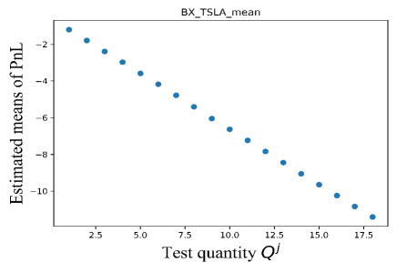
(a) BX mean with R-squared $R^{2}=0.99$

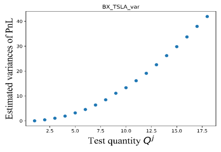
(b) BX var with R-squared $R^{2}=0.94$

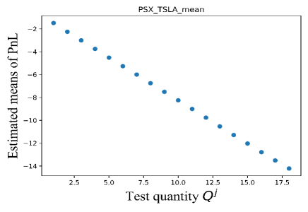
(c) PSX mean with R-squared $R^{2}=0.99$

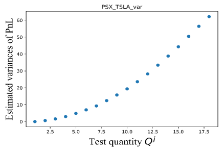
(d) PSX var

(e) NASDAQ mean with R-squared $R^{2}=0.99$

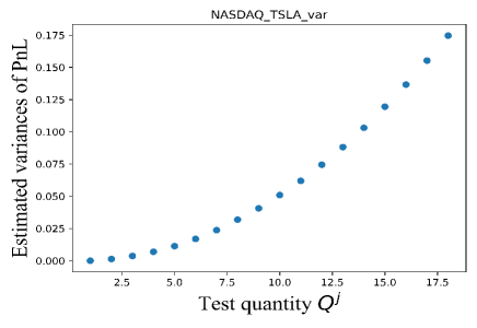
(f) NASDAQ var with R-squared $R^{2}=0.93$

Figure 5: The estimated means and variances of PnL for Tesla stock at different venues, as $Q^{j}$ varies. A clear linear relationship prevails for mean and a linear relationship for variance roughly holds. This is an empirical justification for our linear form approximation Eq. (29) and Eq. (30).

where $\omega>0$ is a positive constant to guarantee that the variance is well-defined. This formulation captures both the linear and the quadratic effect of the trading quantity in each venue on the PnL. These assumptions are supported by empirical observations from real data. See the discussion in Section 1 and Figures 1, 5 for the details.

5.2 A Synthetic Example

In this section, we first briefly showcase the superiority of RISE and RISE++ solving the SOR problem using synthetic data.

For simplicity, we consider only non-negative integer allocations of $S$ orders into $d$ venues. Throughout the experiments, we set the risk-aversion parameter $\rho=2$ and vary the choices of $d$ and $S$. We set $\omega=1$ and scale the action vectors accordingly so that the norms of actions are less than one.

Implementation Details: We note that when implementing RISE, rather than strictly following (8) and (9) to decide the length of exploration phase, we set $n=\lceil dT^{2/3}\rceil$ in the experiments for practical convenience. Also, when implementing RISE++, we set

$$n_{\ell,a}=\left\lceil 0.0001\cdot\frac{d^{3}\log(d)Q_{\ell}^{*}(a)}{\varepsilon_{\ell}^{2}}\log^{2}\left(KT^{2}\right)\right\rceil$$

rather than strictly follow (21). Moreover, we regularize the design matrix as $V_{(\ell)}=\sum_{a\in\mathcal{A}_{\ell}}n_{\ell,a}aa^{\top}+I_{d}$ to avoid singularity issue for RISE++.

To generate problem instances, we randomly sample coefficients from multivariate normal distribution.

Criterion and Benchmark Algorithms: In view of the connection between expected regret (cf. (5)) and intermediate regret established in Sani et al. (2012), we use the intermediate regret $\tilde{R}$ as a performance measure of different algorithms.

We compare RISE and RISE++ with two algorithms proposed by Sani et al. (2012) for the MAB problem. The first one is a variation of the UCB policy (referred to as UCB(MAB)) and the second is a variation of the exploration-and-exploitation policy (referred to as ExpExp(MAB)). To apply these two algorithms to the SOR problem, we simply let all non-negative integer allocations of $S$ orders into $d$ venues be the whole action space. The implementations of the UCB(MAB) and ExpExp(MAB) strictly follow the descriptions in Sani et al. (2012).

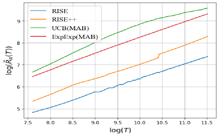
(a) $d=4,S=4,K=35$.

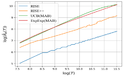
(b) $d=5,S=4,K=70$.

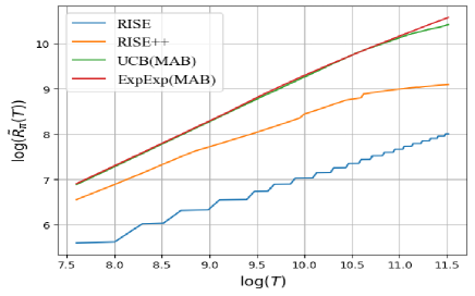
(c) $d=6,S=4,K=126$.

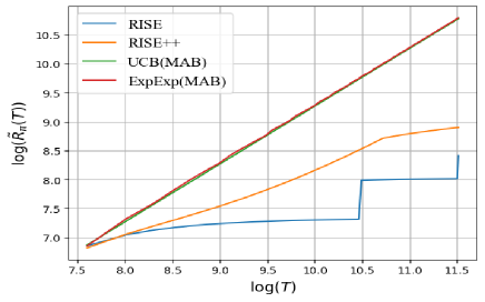
(d) $d=6,S=8,K=1287$.

Figure 2: Intermediate regrets of different algorithms over $T$. RISE and RISE++ outperform the benchmark algorithms.

Numerical Performance and Discussion: The regrets depicted in Figure 2(a) through Figure 2(d) are presented on a logarithmic scale. It is evident that RISE and RISE++ have the best empirical performances in all scenarios. Next, we observe in Figure 2(a) and 2(b) that when action space is relatively small ($K=35$ or $K=70$), the UCB(MAB) still exhibits a logarithmic regret growth rate, with large leading constant terms. Furthermore, through Figure 2(a) to 2(d), the performances of both UCB(MAB) and ExpExp(MAB) get worse as $K$ grows. Figure 2(d) shows that regrets of them grow linearly when the action space is large ($K=1287$). Specifically, since the length of its exploration phase is $K(T/14)^{2/3}$, UCB(ExpExp) will uniformly explore over the whole horizon when $K$ is large. On the contrary, RISE and RISE++ are able to fully utilize the linear structure of the problem and their regret growth rates do not rely on $K$, the size of action space. Therefore, RISE and RISE++ are especially competent for tasks with a huge action space.

5.3 A Numerical Study Based on the NASDAQ ITCH Dataset

Undoubtedly, the actual performance of algorithms is susceptible to the environment specification. In this section, we conduct a numerical study using the NASDAQ ITCH dataset to extract model parameters and evaluate the assumptions made in the framework. This approach ensures that the results of our study are representative of actual financial decision-making scenarios, and can be used to make more informed decisions in practice.

Data Source: Our numerical study is based on historical order book messages from three exchanges at NASDAQ on March 27, 2019. The data is publicly available (NASDAQ ITCH Data 2022). We only use data from 11:00 to 13:00, since the market is usually more stable during this period of time. We reconstruct the LOB from the message-level data using tools developed by Bernasconi-De-Luca et al. (2021). We call the configuration of the LOB at a particular moment the snapshot of the LOB. Each snapshot contains five queues on both the ask and bid side. This dataset consists of 3 lit-pool venues: NASDAQ BX (BX), NASDAQ PSX (PSX) and The Nasdaq Stock Market (NASDAQ). Each of them is a stock exchange with different liquidity incentives. To be specific, NASDAQ has the conventional price/time matching mechanism, while PSX uses a price/pro-rata allocation rule and BX has an inverted pricing model. More details can be found at e.g., Nasdaq (2022a, b, 2017).

Liquidity Simulation: The sampling procedure for estimation works as follows. For a given stock, we group all the LOB snapshots from 11:00 to 13:00 to 60 2-min buckets. To estimate the PnL of submitting market orders to venue $j$, we sample uniformly over time one snapshot at each venue $j$ from each bucket, with different values of test quantity $Q^{j}$. Let $p^{\texttt{bid},j}_{t,i}$ be the $i$th best bid price on the LOB snapshot at time $t$, and let $\bar{q}^{\texttt{bid},j}_{t,i}$ be the corresponding queue size. We split $Q^{j}$ orders to the five queues, with as many orders to the more favorable prices as possible. To be precise, let $q^{\texttt{bid},j}_{t,i}\in[0,\bar{q}^{\texttt{bid},j}_{t,i}]$ be the size of the market order submitted to the $i$th queue. We have $\sum_{i=1}^{5}q^{\texttt{bid},j}_{t,i}=Q^{j}$. Also, $q^{\texttt{bid},j}_{t,i}>0$ only when $\sum_{i^{\prime}=1}^{i-1}q^{\texttt{bid},j}_{t,i^{\prime}}<Q^{j}$ for $2\leq i\leq 5$. Note that due to the nature of the problem, we do not need to set $Q^{j}$ too large so that the orders in the bid queues are not enough to fulfill. We denote $p^{\texttt{mid-price},j}_{t}$ the mid-price of the $j$th venue. Then the relative PnL of market orders is defined to be

$$\sum_{i=1}^{5}p^{\texttt{bid},j}_{t,i}q^{\texttt{bid},j}_{t,i}-p^{\texttt{mid-price},j}_{t}\cdot Q^{j},$$ (31)

against the benchmark level $p^{\texttt{mid-price},j}_{t}\cdot Q^{j}$. See Figure 3 for visualization.

To sample uniformly over time we first uniformly sample a time point in the bucket, and then match it with the closest snapshot within the bucket. We note that this sampled time point is used across three venues. Finally, we obtain the empirical mean and variance of PnL (cf. Eq. (31)) over 60 buckets.

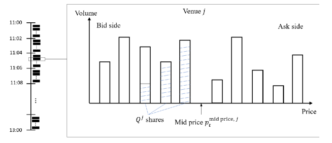
Figure 3: Visualization of the sampling procedure. We sample one snapshot of the LOB from each bucket uniformly over time. Then we obtain the empirical mean and variance PnL (cf. Eq. (31)) over 60 buckets.

For dark pools, we do not have access to any data to simulate from. So based on the estimated coefficients of lit pools, we randomly generate moments of dark pools such that they generally have higher but more volatile returns. Also, we make sure that the first two moments of dark pools are on a scale comparable to the lit pools. For this experiment, we set to sell $S=10$ shares over $d=5$ venues. Table 1 in Online Companion 8 reports the parameters we used for our experiments. The rows $p$ and $\tilde{p}$ stand for the coefficients of the mean of the PnL for each venue, and it is estimated by regressing PnL on $Q^{j}$ and ${(Q^{j})}^{2}$. Similarly, the rows $\sigma^{2}$ and $\tilde{\sigma}^{2}$ stand for the estimated coefficients of the variance.

Validation of Assumption (29) and (30): Figure 5 in Online Companion 8 plots the estimated means and variances of PnL for Tesla stock at different venues, as $Q^{j}$ varies. We observe strong empirical evidence for a linear relationship between the mean trading profit and $Q^{j}$ for the considered scale of $Q^{j}$, which supports the approximation in Eq. (29). Also, there is approximately a quadratic relationship between the variance of trading profit and $Q^{j}$. Essentially, this critically hinges on the fact that we are trading a volume that will not eat up the best bid queue in a liquid market.

Numerical Performance: Figure 4 shows that RISE and RISE++ still exhibit a sublinear regret growth in this more realistic experiment. Interestingly, we find that UCB(MAB) also performs well in this example. ExpExp(MAB) suffers a linear regret because its designed exploration phase scales as $K$, which will be excessively long in this case.

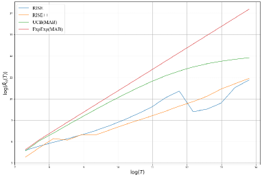
Figure 4: Intermediate regret. RISE and RISE++ exhibit sublinear regret in the experiment based on the NASDAQ ITCH dataset.

6 Conclusion

Linear bandit is a natural setting in online decision-making to handle large action sets which appear in many financial applications, meanwhile, mean-variance is one of the most popular criteria used by investors to balance the trade-off between the risk and expected returns of their investments. To the best of our knowledge, this is the first theoretical work that studies linear bandits under mean-variance framework. The numerical experiment justifies the linear approximation for the SOR problem, validates our theoretical finding, and demonstrates their strong performances compared with existing algorithms for the SOR problem. Motivated by other practical considerations in financial decision-making problems, future directions include risk-sensitive frameworks with other risk measures (Simchi-Levi et al. 2023b, Coache and Jaimungal 2023), delayed feedback (Pike-Burke et al. 2018, Bistritz et al. 2022, Blanchet et al. 2023), and non-stationary environment (Zhu and Zheng 2020, Cheung et al. 2022, Simchi-Levi et al. 2023a).

Electronic Companion

7 Omitted Proofs

7.1 Proof of Proposition 3.2

From Eq. (21.1) of Lattimore and Szepesvári [2020]), we have for any fixed $n,$ $\delta>0$, and every $a\in\mathcal{A},$

$$\mathbf{Pr}\left[{\left|\langle\hat{\theta}_{n}-\theta_{*},a\rangle\right|\geq\sigma_{\max}\sqrt{2\|a\|^{2}_{V^{-1}_{n}}\log\left(2\delta^{-1}\right)}}\right]\leq\delta.$$ (32)

Then from Theorem 1 of Hsieh et al. [2019], we have for any fixed $n,$ $\delta>0$, and every $a\in\mathcal{A},$

$$\left|\left\langle{\hat{\phi}_{n}-\phi_{*},a}\right\rangle\right|\leq C_{3}\left\|a\right\|_{V_{n}^{-1}}d\sqrt{\log(d)}\log(2\delta^{-1})\ .$$ (33)

By a union bound over (32) and (33), we have for any fixed $n,$ $\delta>0$, and every $a\in\mathcal{A},$ it holds with probability at least $1-\delta$, that

$$\left|\left\langle{a,\phi_{*}-\rho\theta_{*}}\right\rangle-\left\langle{a,\hat{\phi}_{n}-\rho\hat{\theta}_{n}}\right\rangle\right|$$

$$\leq \rho\left|\left\langle{a,\theta_{*}-\hat{\theta}_{n}}\right\rangle\right|+\left|\left\langle{a,\phi_{*}-\hat{\phi}_{n}}\right\rangle\right|$$

$$\leq \left\|a\right\|_{V_{n}^{-1}}\rho\sigma_{\max}\sqrt{2\log\left(4\delta^{-1}\right)}+C_{3}\left\|a\right\|_{V_{n}^{-1}}d\sqrt{\log(d)}\log(4\delta^{-1})$$

$$\leq \left\|a\right\|_{V_{n}^{-1}}\tilde{C}d\sqrt{\log{(d)}}\log({\delta^{-1}})\ ,$$ (34)

where the second step follows from the triangle inequality and the last step follows from the definition of $\tilde{C}$, c.f. Eq. (6).

Now recall the definition of $n_{a}$ in (8), we have

$$V_{n}= \sum_{a\in\mathcal{A}}n_{a}aa^{\top}=\sum_{a\in\mathcal{A}}\left\lceil\frac{\tilde{C}^{2}\log^{2}\left(\delta^{-1}\right)d^{2}\log{(d)}g(Q^{*})Q^{*}(a)}{\varepsilon^{2}}\right\rceil aa^{\top}$$

$$\succeq \sum_{a\in\mathcal{A}}\frac{\tilde{C}^{2}\log^{2}\left(\delta^{-1}\right)d^{2}\log{(d)}g(Q^{*})Q^{*}(a)}{\varepsilon^{2}}aa^{\top}$$

$$= \frac{\tilde{C}^{2}\log^{2}\left(\delta^{-1}\right)d^{2}\log{(d)}g(Q^{*})}{\varepsilon^{2}}\sum_{a\in\mathcal{A}}Q^{*}(a)aa^{\top}\ ,$$ (35)

where we denote by $B\succeq 0$ if the matrix $B$ is positive semi-definite. Hence, we arrive at

$$\left\|a\right\|_{V_{n}^{-1}}= \sqrt{a^{\top}V_{n}^{-1}a}\leq\sqrt{\frac{\varepsilon^{2}a^{\top}(\sum_{a\in\mathcal{A}}Q^{*}(a)aa^{\top})^{-1}a}{\tilde{C}^{2}\log^{2}\left(\delta^{-1}\right)d^{2}\log(d)g(Q^{*})}}$$

$$\leq \frac{\varepsilon}{\tilde{C}d\sqrt{\log(d)}\log\left(\delta^{-1}\right)}\ ,$$ (36)

where the last step follows from the fact that $Q^{*}$ is an optimal solution to (1). The statement follows by combining (34) and (36).

7.2 Proof of Proposition 3.3

For ease of notation, in this section we omit the superscript $\pi$ for the reward $X_{t}^{\pi}$ and action taken $A_{t}^{\pi}$ where no confusion arises.

The idea is to decompose the expected regret in time. The instantaneous expected regret at round $t,t\geq 2$ can be written as

$$\mathbb{E}\left[{r_{\pi}(t+1)}\right]$$ (37)

$$= \mathbb{E}\left[{\mathcal{R}_{\pi}(t+1)-\mathcal{R}_{\pi}(t)}\right]$$

$$= \mathbb{E}\left[{\xi_{\pi}(t+1)-\xi_{\pi}(t)}\right]-\left(\left\langle{\phi_{*},a_{*}}\right\rangle+\omega-\rho\left\langle{\theta_{*},a_{*}}\right\rangle\right)$$

$$= \mathbb{E}\left[{\sum_{s=1}^{t+1}\left(X_{s}^{\pi}-\frac{1}{t+1}\sum_{\tau=1}^{t+1}X_{\tau}^{\pi}\right)^{2}-\rho\sum_{s=1}^{t+1}X^{\pi}_{s}-\sum_{s=1}^{t}\left(X_{s}^{\pi}-\frac{1}{t}\sum_{\tau=1}^{t}X_{\tau}^{\pi}\right)^{2}+\rho\sum_{s=1}^{t}X^{\pi}_{s}}\right]-\left(\left\langle{\phi_{*},a_{*}}\right\rangle+\omega-\rho\left\langle{\theta_{*},a_{*}}\right\rangle\right)$$

$$= \mathbb{E}\left[{\frac{1}{t(t+1)}\left(tX_{t+1}-\sum_{s=1}^{t}X_{t}\right)^{2}-\rho X_{t+1}}\right]-\left(\left\langle{\phi_{*},a_{*}}\right\rangle+\omega-\rho\left\langle{\theta_{*},a_{*}}\right\rangle\right),$$

where the last equation is due to the following algebraic fact.

Lemma 7.1

Denote by $\bar{x}_{n}=\frac{1}{n}\sum_{k=1}^{n}x_{k}$ and let $S_{n}=\sum_{k=1}^{n}\left(x_{k}-\bar{x}_{n}\right)^{2}$. Then we have

$$S_{n+1}=S_{n}+\frac{\left(nx_{n+1}-n\bar{x}_{n}\right)^{2}}{n(n+1)}\ .$$ (38)

Continuing from (37), we have

$$\mathbb{E}\left[{r_{\pi}(t+1)}\right]$$ (39)

$$= \mathbb{E}\left[{\frac{1}{t(t+1)}\left(t\left\langle{\theta_{*},A_{t+1}}\right\rangle+t\eta_{t+1}(A_{t+1})-\sum_{s=1}^{t}\left(\left\langle{\theta_{*},A_{s}}\right\rangle+\eta_{s}(A_{s})\right)\right)^{2}}\right]-\rho\mathbb{E}\left[{\left\langle{\theta_{*},A_{t+1}}\right\rangle}\right]-\left(\left\langle{\phi_{*},a_{*}}\right\rangle+\omega-\rho\left\langle{\theta_{*},a_{*}}\right\rangle\right)$$

$$= \frac{1}{t(t+1)}\mathbb{E}\left[{\left(t\left\langle{\theta_{*},A_{t+1}}\right\rangle-\sum_{s=1}^{t}\left\langle{\theta_{*},A_{s}}\right\rangle\right)^{2}}\right]+\frac{1}{t(t+1)}\mathbb{E}\left[{\left(t\eta_{t+1}(A_{t+1})-\sum_{s=1}^{t}\eta_{s}(A_{s})\right)^{2}}\right]$$

$$-\rho\mathbb{E}\left[{\left\langle{\theta_{*},A_{t+1}}\right\rangle}\right]-\left(\left\langle{\phi_{*},a_{*}}\right\rangle+\omega-\rho\left\langle{\theta_{*},a_{*}}\right\rangle\right)$$

$$+\frac{2}{t(t+1)}\mathbb{E}\left[{\left(t\left\langle{\theta_{*},A_{t+1}}\right\rangle-\sum_{s=1}^{t}\left\langle{\theta_{*},A_{s}}\right\rangle\right)\left(t\eta_{t+1}(A_{t+1})-\sum_{s=1}^{t}\eta_{s}(A_{s})\right)}\right]\ .$$

We proceed to deal with each term in (39) respectively.

• For the first three terms, we note that

  $$\frac{1}{t(t+1)}\mathbb{E}\left[{\left(t\left\langle{\theta_{*},A_{t+1}}\right\rangle-\sum_{s=1}^{t}\left\langle{\theta_{*},A_{s}}\right\rangle\right)^{2}}\right]+\frac{1}{t(t+1)}\mathbb{E}\left[{\left(t\eta_{t+1}(A_{t+1})-\sum_{s=1}^{t}\eta_{s}(A_{s})\right)^{2}}\right]$$

  $$-\rho\mathbb{E}\left[{\left\langle{\theta_{*},A_{t+1}}\right\rangle}\right]-\left(\left\langle{\phi_{*},a_{*}}\right\rangle+\omega-\rho\left\langle{\theta_{*},a_{*}}\right\rangle\right)$$

  $$= \frac{1}{t(t+1)}\mathbb{E}\left[{\left(t\left\langle{\theta_{*},A_{t+1}}\right\rangle-\sum_{s=1}^{t}\left\langle{\theta_{*},A_{s}}\right\rangle\right)^{2}}\right]+\frac{1}{t(t+1)}\sum_{i=1}^{t}\sum_{j=1}^{t}\left(\mathbb{E}\left[{\eta_{t+1}^{2}}\right]-\mathbb{E}\left[{\eta_{i}\eta_{t+1}}\right]-\mathbb{E}\left[{\eta_{j}\eta_{t+1}}\right]+\mathbb{E}\left[{\eta_{i}\eta_{j}}\right]\right)$$

  $$-\rho\mathbb{E}\left[{\left\langle{\theta_{*},A_{t+1}}\right\rangle}\right]-\left(\left\langle{\phi_{*},a_{*}}\right\rangle+\omega-\rho\left\langle{\theta_{*},a_{*}}\right\rangle\right)$$

  $$= \mathbb{E}\left[{\frac{1}{t(t+1)}\left(t\left\langle{\theta_{*},A_{t+1}}\right\rangle-\sum_{s=1}^{t}\left\langle{\theta_{*},A_{s}}\right\rangle\right)^{2}+\frac{1}{t(t+1)}\left(t^{2}\left(\left\langle{\phi_{*},A_{t+1}}\right\rangle+\omega\right)+\sum_{s=1}^{t}\left(\left\langle{\phi_{*},A_{s}}\right\rangle+\omega\right)\right)}\right]$$

  $$-\rho\mathbb{E}\left[{\left\langle{\theta_{*},A_{t+1}}\right\rangle}\right]-\left(\left\langle{\phi_{*},a_{*}}\right\rangle+\omega-\rho\left\langle{\theta_{*},a_{*}}\right\rangle\right)$$

  $$\leq \mathbb{E}\left[{\frac{1}{t(t+1)}\left(\sum_{s=1}^{t}\left(\left\langle{\theta_{*},A_{t+1}-A_{s}}\right\rangle\right)^{2}\sum_{s=1}^{t}1\right)+\frac{1}{t(t+1)}\left(t^{2}\left(\left\langle{\phi_{*},A_{t+1}}\right\rangle+\omega\right)+\sum_{s=1}^{t}\left(\left\langle{\phi_{*},A_{s}}\right\rangle+\omega\right)\right)}\right]$$

  $$-\rho\mathbb{E}\left[{\left\langle{\theta_{*},A_{t+1}}\right\rangle}\right]-\left(\left\langle{\phi_{*},a_{*}}\right\rangle+\omega-\rho\left\langle{\theta_{*},a_{*}}\right\rangle\right)$$

  $$= \mathbb{E}\left[{\frac{1}{(t+1)}\sum_{s=1}^{t}\left(\left\langle{\theta_{*},A_{t+1}-A_{s}}\right\rangle\right)^{2}+\frac{1}{t(t+1)}\left(t^{2}\left\langle{\phi_{*},A_{t+1}-a_{*}}\right\rangle+\sum_{s=1}^{t}\left\langle{\phi_{*},A_{s}-a_{*}}\right\rangle\right)-\rho\left\langle{\theta_{*},A_{t+1}-a_{*}}\right\rangle}\right]$$

  $$= \mathbb{E}\left[{\frac{1}{(t+1)}\sum_{s=1}^{t}\left(\left\langle{\theta_{*},A_{t+1}-A_{s}}\right\rangle\right)^{2}+\left\langle{\phi_{*}-\rho\theta_{*},A_{t+1}-a_{*}}\right\rangle+\frac{1}{t(t+1)}\sum_{s=1}^{t}\left\langle{\phi_{*},A_{s}-A_{t+1}}\right\rangle}\right]\ .$$ (42)

  Equation (• ‣ 7.2) follows by noting that $\mathbb{E}\left[{\eta_{i}(A_{i})\eta_{j}(A_{j})}\right]=0$ for $i\neq j$. Inequality (• ‣ 7.2) follows from Cauchy. Let us observe that only the first two terms in (42) contribute significantly to the regret. Since,

  $$\mathbb{E}\left[{\sum_{t=1}^{T}\frac{1}{t(t+1)}\sum_{s=1}^{t}\left\langle{\phi_{*},A_{s}-A_{t+1}}\right\rangle}\right] \leq 2\sum_{t=1}^{T}\frac{1}{(t+1)}=O(\log\left({T}\right))\ .$$

• Regarding the last term in (39), which corresponds to the variance term caused by the accumulated noise, first we note that

  $$\mathbb{E}\left[{\left({t\left\langle{\theta_{*},A_{t+1}}\right\rangle-\sum_{s=1}^{t}\left\langle{\theta_{*},A_{s}}\right\rangle}\right)\eta_{t+1}(A_{t+1})}\right]=\mathbb{E}\left[{\left({t\left\langle{\theta_{*},A_{t+1}}\right\rangle-\sum_{s=1}^{t}\left\langle{\theta_{*},A_{s}}\right\rangle}\right)\mathbb{E}\left[{\eta_{t+1}(A_{t+1})\mid\mathcal{F}_{t}}\right]}\right]=0\ .$$ (43)

  Also, we have

  $$\frac{2}{t(t+1)}\mathbb{E}\left[{\left(\sum_{s=1}^{t}\left\langle{\theta_{*},A_{s}-A_{t+1}}\right\rangle\right)\sum_{s=1}^{t}\eta_{s}(A_{s})}\right]$$

  $$\leq \frac{2}{t(t+1)}2t\mathbb{E}\left[{\left|\sum_{s=1}^{t}\eta_{s}(A_{s})\right|}\right]$$

  $$= \frac{4}{t+1}\int_{0}^{\infty}\mathbf{Pr}\left[{\left|\sum_{s=1}^{t}\eta_{s}(A_{s})\right|>u}\right]du$$

  $$\leq \frac{4}{t+1}\int_{0}^{\infty}2\exp\left({-\frac{u^{2}}{2t\sigma_{\max}^{2}}}\right)du$$ (45)

  $$= 4\sqrt{2\pi\sigma_{\max}^{2}}\frac{\sqrt{t}}{t+1}\ .$$ (46)

  For (• ‣ 7.2), we recall the fact that $\|\theta_{*}\|_{2}\leq 1,\|a\|_{2}\leq 1$. Inequality (45) follows since the noises are sub-Gaussian.

Putting everything together, we arrive at

$$\mathbb{E}\left[{\mathcal{R}_{\pi}(T)}\right] \leq \sum_{t=1}^{T-1}\mathbb{E}\left[{\frac{1}{(t+1)}\sum_{s=1}^{t}\left(\left\langle{\theta_{*},A_{t+1}-A_{s}}\right\rangle\right)^{2}+\left\langle{\phi_{*}-\rho\theta_{*},A_{t+1}-a_{*}}\right\rangle}\right]$$ (47)

$$+\sum_{t=1}^{T}\left({4\sqrt{2\pi\sigma_{\max}^{2}}\frac{\sqrt{t}}{t+1}+\frac{1}{t+1}}\right)$$

$$= \sum_{t=1}^{T-1}\mathbb{E}\left[{\frac{1}{(t+1)}\sum_{s=1}^{t}\left(\left\langle{\theta_{*},A_{t+1}-A_{s}}\right\rangle\right)^{2}+\left\langle{\phi_{*}-\rho\theta_{*},A_{t+1}-a_{*}}\right\rangle}\right]+O\left({\sqrt{T}}\right)\ .$$

7.3 Proof of Proposition 4.3

By virtue of Eq. (20.3) in Lattimore and Szepesvári [2020], in phase $\ell$, for given $\delta_{\ell}>0$ we have

$$\mathbf{Pr}\left[{\left\|\hat{\theta}_{(\ell)}-\theta_{*}\right\|_{V_{(\ell)}}\leq 8\sigma_{\max}^{2}\sqrt{d+\log\left(\frac{1}{\delta_{\ell}}\right)}}\right]\geq 1-\delta_{\ell}.$$ (48)

Choosing $\delta_{\ell}=\frac{\delta}{2\ell^{2}}$ and applying the union bound over $\ell\in\mathbb{N}$, we see that

$$\mathbf{Pr}\left[{\left\|\hat{\theta}_{(\ell)}-\theta_{*}\right\|_{V_{(\ell)}}\leq 8\sigma_{\max}^{2}\sqrt{d+\log\left(\frac{2T^{2}}{\delta}\right)},~{}\forall\ell\in\mathbb{N}}\right]\geq 1-\delta.$$ (49)

Also, from Theorem 1 of Hsieh et al. [2019], for any fixed $\delta>0$, we have

$$\mathbf{Pr}\left[{\left\|\hat{\phi}_{(\ell)}-\phi_{*}\right\|_{V_{(\ell)}}\leq C_{4}d\sqrt{\log(d)}\log(\frac{T}{\delta}),\forall\ell\in\mathbb{N}}\right]\geq 1-\delta.$$ (50)

Combining the above two concentration results we know that for given $\delta>0$, with probability at least $1-\delta$,

$$\left|\left\langle{\rho\theta_{*}-\phi_{*}-\left(\rho\hat{\theta}_{(\ell)}-\hat{\phi}_{(\ell)}\right),a}\right\rangle\right| \leq \left\|\rho\theta_{*}-\phi_{*}-\left(\rho\hat{\theta}_{(\ell)}-\hat{\phi}_{(\ell)}\right)\right\|_{V_{(\ell)}}\left\|a\right\|_{V_{(\ell)}^{-1}}$$ (51)

$$\leq \left(\rho\left\|\hat{\theta}_{(\ell)}-\theta_{*}\right\|_{V_{(\ell)}}+\left\|\hat{\phi}_{(\ell)}-\phi_{*}\right\|_{V_{(\ell)}}\right)\left\|a\right\|_{V_{(\ell)}^{-1}}$$

$$\leq \left(\rho 8\sigma_{\max}^{2}\sqrt{d+\log\left(\frac{2T^{2}}{\delta}\right)}+C_{4}d\sqrt{\log(d)}\log(\frac{T}{\delta})\right)\left\|a\right\|_{V_{(\ell)}^{-1}}$$

$$\leq \hat{C}d\sqrt{\log(d)}\log\left(\frac{T}{\delta}\right)\left\|a\right\|_{V_{(\ell)}^{-1}}$$

for any $\ell\in\mathbb{N}$. Applying the union bound over the action set $\mathcal{A}$, we arrive at

$$\mathbf{Pr}\left[{\left|\left\langle{\rho\theta_{*}-\phi_{*}-\left(\rho\hat{\theta}_{(\ell)}-\hat{\phi}_{(\ell)}\right),a}\right\rangle\right|\leq\hat{C}d\sqrt{\log(d)}\log\left(\frac{KT}{\delta}\right)\left\|a\right\|_{V_{(\ell)}^{-1}},\forall\ell\in\mathbb{N}\text{ and }\forall a\in\mathcal{A}}\right]\geq 1-\delta.$$ (52)

Recalling the definition of $n_{\ell,a}$ in (21), we have

$$V_{(\ell)}=\sum_{a\in\mathcal{A}_{\ell}}n_{\ell,a}aa^{\top} = \sum_{a\in\mathcal{A}_{\ell}}\left\lceil\hat{C}^{2}\frac{d^{2}g_{\ell}(Q^{*}_{\ell})\log(d)Q_{\ell}^{*}(a)}{\varepsilon_{\ell}^{2}}\log^{2}\left(\frac{KT}{\delta}\right)\right\rceil aa^{\top}$$

$$\succeq \hat{C}^{2}\frac{d^{2}g_{\ell}(Q^{*}_{\ell})\log(d)}{\varepsilon_{\ell}^{2}}\log^{2}\left(\frac{KT}{\delta}\right)\sum_{a\in\mathcal{A}_{\ell}}Q_{\ell}^{*}(a)aa^{\top}.$$

Hence, we see that

$$\left\|a\right\|_{V_{(\ell)}^{-1}} = \sqrt{a^{\top}V_{(\ell)}^{-1}a}\leq\frac{\varepsilon_{\ell}}{\hat{C}d\sqrt{\log{d}}}\frac{1}{\log\left(\frac{KT}{\delta}\right)}\sqrt{\frac{a^{\top}\left(\sum_{a\in\mathcal{A}_{\ell}}Q_{\ell}^{*}(a)aa^{\top}\right)^{-1}a}{g_{\ell}(Q^{*}_{\ell})}}$$ (53)

$$\leq \frac{\varepsilon_{\ell}}{\hat{C}d\sqrt{\log{d}}}\frac{1}{\log\left(\frac{KT}{\delta}\right)},$$

where the last inequality follows from the fact that $Q^{*}_{\ell}(\cdot)$ is an optimal solution to (20). By combining (51) and (53), we conclude the desired result.

7.4 Proof of Proposition 4.4

We denote by $G_{\ell}^{a}$ the event that the MV estimate for action $a$ in phase $\ell$ deviates from the true value no more than $\varepsilon_{\ell}$, namely,

$$G_{\ell}^{a}=\left\{\left|\left\langle{\rho\hat{\theta}_{(\ell)}-\hat{\phi}_{(\ell)}-\left(\rho\theta_{*}-\phi_{*}\right),a}\right\rangle\right|\leq\varepsilon_{\ell}\right\}.$$

We say the good event happens if for any action $a$ in exploration basis $\mathcal{A}_{\ell}$ in all phases, $G_{\ell}^{a}$ happens. I.e., we let $G=\underset{\ell}{\mathbin{\scalebox{1.66}{$\cap$}}}\underset{a\in\mathcal{A}_{\ell}}{\mathbin{\scalebox{1.66}{$\cap$}}}G_{a}^{\ell}$. By Lemma 4.3, we know the event $G$ happens with probability at least $1-\delta$.

We first observe that if $G$ happens, then in phase $\ell$, the optimal action $a_{*}$ will not be eliminated at step (4) in Algorithm 2. To see this, suppose in phase $\ell$, the optimal action $a_{*}$ were eliminated by some suboptimal action $b$, which would mean $\exists~{}b\in\mathcal{A}_{\ell}$ such that

$$\left\langle{\rho\hat{\theta}_{(\ell)}-\hat{\phi}_{(\ell)},b-a_{*}}\right\rangle>2\varepsilon_{\ell}$$ (54)

$$\Leftrightarrow~{} \langle\rho\hat{\theta}_{(\ell)}-\hat{\phi}_{(\ell)},b\rangle-\varepsilon_{\ell}>\langle\rho\hat{\theta}_{(\ell)}-\hat{\phi}_{(\ell)},a_{*}\rangle+\varepsilon_{\ell}.$$

Since $G$ happens, we have

$$\langle\rho\theta_{*}-\phi_{*},b\rangle\geq\langle\rho\hat{\theta}_{(\ell)}-\hat{\phi}_{(\ell)},b\rangle-\varepsilon_{\ell}~{}~{}\text{and}~{}~{}\langle\rho\hat{\theta}_{(\ell)}-\hat{\phi}_{(\ell)},a_{*}\rangle+\varepsilon_{\ell}\geq\langle\rho\theta_{*}-\phi_{*},a_{*}\rangle,$$

which, combined with (54), leads to the contradiction $\langle\rho\theta_{*}-\phi_{*},b\rangle>\langle\rho\theta_{*}-\phi_{*},a_{*}\rangle$.

Next, we argue that provided the good event $G$ happens, a suboptimal action $a$ with gap $\Delta_{a}$ will be eliminated before $\ell_{a}=\min\{\ell:2\varepsilon_{\ell}<\Delta_{a}\}$. Indeed, at step (3) of phase $\ell+1$, the estimated MV gap of action $a$ based on estimators in the previous phase $\ell$ is no more than $2\varepsilon_{\ell}$, i.e.,

$$\max_{b\in\mathcal{A}_{\ell+1}}\left\langle{\rho\hat{\theta}_{(\ell)}-\hat{\phi}_{(\ell)},b-a}\right\rangle\leq 2\varepsilon_{\ell}=4\varepsilon_{l+1}.$$

In particular, the optimal action $a_{*}$ remains in $\mathcal{A}_{\ell+1}$. Hence, we have

$$\left\langle{\rho\hat{\theta}_{(\ell)}-\hat{\phi}_{(\ell)},a_{*}-a}\right\rangle\leq 2\varepsilon_{\ell}$$ (55)

for any suboptimal action $a\in\mathcal{A}_{\ell+1}$. On the other hand, the event $G$ implies that $-\varepsilon_{\ell}\leq\left\langle{\rho\hat{\theta}_{(\ell)}-\hat{\phi}_{(\ell)}-\left(\rho\theta_{*}-\phi_{*}\right),a}\right\rangle\leq\varepsilon_{\ell}$ and $-\varepsilon_{\ell}\leq\left\langle{\rho\hat{\theta}_{(\ell)}-\hat{\phi}_{(\ell)}-\left(\rho\theta_{*}-\phi_{*}\right),a_{*}}\right\rangle\leq\varepsilon_{\ell}$ hold, which means

$$-2\varepsilon_{\ell}\leq\left\langle{\rho\theta_{*}-\phi_{*},a_{*}-a}\right\rangle-\left\langle{\rho\hat{\theta}_{(\ell)}-\hat{\phi}_{(\ell)},a_{*}-a}\right\rangle\leq 2\varepsilon_{\ell}.$$ (56)

Combining (55) and (56) yields that

$$\Delta_{a}=\left\langle{\rho\theta_{*}-\phi_{*},a_{*}-a}\right\rangle\leq 4\varepsilon_{\ell}=2\varepsilon_{\ell+1}.$$

Therefore, the true MV gap incurred by a suboptimal action in $\mathcal{A}_{\ell}$ is at most $2\varepsilon_{\ell}$. In other words, when $G$ happens, a suboptimal action $a$ with gap $\Delta_{a}$ will be eliminated before phase $\ell_{a}=\min\{\ell\geq 1:2\varepsilon_{\ell}<\Delta_{a}\}=\lceil\log_{2}(2/\Delta_{a})\rceil$. This also indicates

$$\varepsilon_{\ell_{a}}\geq\frac{\Delta_{a}}{4}\,.$$ (57)

By setting $\delta={1}/{T}$, we can therefore bound the quantity $\mathbb{E}\left[{\tau_{a}(T)}\right]$:

$$\mathbb{E}\left[{\tau_{a}(T)}\right] \leq \frac{1}{T}\cdot T+(1-\frac{1}{T})\sum_{\ell=1}^{\ell_{a}}n_{\ell,a}$$

$$\leq 1+\sum_{\ell=1}^{\ell_{a}}\left\lceil\hat{C}^{2}\frac{d^{2}g_{\ell}(Q_{\ell}^{*})\log(d)Q_{\ell}^{*}(a)}{\varepsilon_{\ell}^{2}}\log^{2}\left(\frac{KT}{\delta}\right)\right\rceil$$

$$\leq 1+\sum_{\ell=1}^{\ell_{a}}\left(\hat{C}^{2}\frac{d^{3}\log(d)Q^{*}_{\ell}(a)}{\varepsilon_{\ell}^{2}}\log^{2}\left(\frac{KT}{\delta}\right)+1\right)$$

$$\leq 1+\hat{C}^{2}d^{3}\log(d)\log^{2}(KT^{2})\sum_{\ell=1}^{\ell_{a}}\frac{Q^{*}_{l}(a)}{\varepsilon_{\ell}^{2}}+\ell_{a}$$

$$\leq 1+\hat{C}^{2}d^{3}\log(d)\log^{2}(KT^{2})\frac{\sum_{\ell=1}^{\ell_{a}}Q^{*}_{l}(a)}{\varepsilon_{\ell_{a}}^{2}}+\log\left(\frac{2}{\Delta_{a}}\right)+1$$

$$\leq 2+\frac{16\hat{C}^{2}d^{3}\log(d)\log^{2}(KT^{2})}{\Delta^{2}_{a}}\left(\sum_{\ell=1}^{\ell_{a}}Q^{*}_{l}(a)\right)+\log\left(\frac{2}{\Delta_{a}}\right)\,.$$

Here, the second last inequality uses the fact that $\epsilon_{l-1}>\epsilon_{l}$ and the last step uses (57). Therefore, noting the simple algebraic fact that $\log\left(2/\Delta\right)<1/\Delta^{2}$ for positive $\Delta$, we conclude that

$$\mathbb{E}\left[{\tau_{a}(T)}\right]\leq O\left(\frac{d^{3}\log(d)\log^{2}(KT)}{\Delta^{2}_{a}}\left(\sum_{\ell=1}^{\ell_{a}}Q^{*}_{l}(a)\right)\right).$$

8 Figures and Tables for Section 5

Table 1: Model parameters used for the experiment

	PSX	BX	NASDAQ	Dark pool 1	Dark pool 2
$p$	- 1.1439	- 1.4709	- 0.07	-0.05	- 0.01
$\tilde{p}$	0.0008	-0.000001	-0.0002	0.0003	0.0002
$\sigma^{2}$	-0.031	- 0.000001	-0.000004	-0.0191	-0.0091
$\tilde{\sigma}^{2}$	0.0391	0.000001	0.00056	0.06	0.05

9 Extension: Risk-aware Contextual Bandit

In many financial applications such as smart order routing, market-making, and intra-day trading, the reward (e.g., profit-and-loss) depends on the real-time market microstructure such as order flow imbalance and volatility [Cont et al., 2014, Hambly et al., 2021]. Motivated by this practical consideration, this section considers the framework of contextual bandit where a random context arrives at each time point, representing the current market condition in the financial applications. The unknown coefficients in the model depend on the realization of the context.

Mathematically, we assume that the context $Z_{t}$ arrives at the beginning of each round $t$ and they are $i.i.d.$ following a categorical distribution $\operatorname{CG}\left({\mathbf{p}}\right)=[p_{1},\cdots,p_{M}]$, which we call the arrival distribution. Upon observing $Z_{t}=c$, we assume that the reward follows

$$X_{t}=\left\langle{A_{t},\theta_{*}^{c}}\right\rangle+\eta_{t}(A_{t}),\quad\text{with}$$

$$\eta_{t}(A_{t})\sim\mathcal{N}\left(0,f(\left\langle{\phi_{*}^{c},A_{t}}\right\rangle)\right),\quad f(\left\langle{\phi_{*}^{c},A_{t}}\right\rangle)=\left\langle{\phi_{*}^{c},A_{t}}\right\rangle+\omega,$$ (59)

where $\omega$ is some constant which ensures the variance is non-negative. Here vectors $\theta_{*}^{c},\phi_{*}^{c}\in\mathbb{R}^{d}$ are unknown parameters with bounded $\ell_{2}$-norm, i.e., $\|\theta_{*}^{c}\|_{2}\leq 1,\|\phi_{*}^{c}\|_{2}\leq\omega,$ so that $f(\left\langle{\phi_{*}^{c},A_{t}}\right\rangle)\in[\sigma_{\min}^{2},\sigma_{\max}^{2}]$. In addition, we assume the action set $\mathcal{A}$ is fixed over time regardless of the current context.

In the presence of contexts, the benchmark policy $\pi^{*}$ is the one that has the knowledge of $\left\{{\theta_{*}^{c}}\right\}_{c=1}^{M},\left\{{\phi_{*}^{c}}\right\}_{c=1}^{M}$ and selects the best action with the smallest mean-variance given the context. Namely, given $Z_{t}=c$, then the best action $a_{t}^{*}$ is the one which attains the best mean-variance, i.e. $a_{t}^{*}=\argmin_{a\in\mathcal{A}}\left\langle{\phi_{*}^{c},a}\right\rangle-\rho\left\langle{\theta_{*}^{c},a}\right\rangle$ .

Algorithm 3 The Contextual Risk-Aware Explore-then-Commit (CRISE) Algorithm.

(1) Given $\mathcal{A}$, find the $G$-optimal design $Q^{*}$ as the solution to

$$\underset{Q(\cdot)}{\operatorname{minimize}}~{}g(Q):=\max_{a\in\mathcal{A}}a^{\top}\left(\sum_{a\in\mathcal{A}}Q(a)aa^{\top}\right)^{-1}a$$

$$\text{s.t.,}~{}\sum_{a\in\mathcal{A}}Q(a)=1\,,\ Q(a)\geq 0~{}~{}~{}\forall a\in\mathcal{A}.$$

(2) For the first $n=dT^{2/3}$ rounds, observe the current context $c$. Select the next action in $N_{(c)}$.

(3) Compute least squares estimates for each $c\in[M]$

$$\hat{\theta}_{n}^{(c)}=\left({\sum_{s=1}^{n}\mathbbm{1}\left[{Z_{s}=c}\right]X_{s}X_{s}^{\top}}\right)^{-1}\sum_{s=1}^{n}\mathbbm{1}\left[{Z_{s}=c}\right]X_{s}A_{s},$$

$$\hat{\phi}_{n}^{(c)}=\left({\sum_{s=1}^{n}\mathbbm{1}\left[{Z_{s}=c}\right]X_{s}X_{s}^{\top}}\right)^{-1}\sum_{s=1}^{n}\mathbbm{1}\left[{Z_{s}=c}\right]f^{-1}\left(\left(X_{s}-\left\langle{\hat{\theta}_{n}^{(c)},\,A_{s}}\right\rangle\right)^{2}\right)A_{s}\ .$$

(4) For the remaining $T-n$ rounds, select the action that maximizes the estimated MV

$$\hat{a}^{*}_{t}=\arg\min_{a\in\mathcal{A}}\left\langle{\hat{\phi}_{n}^{(Z_{t})}-\rho\hat{\theta}_{n}^{(Z_{t})}\ ,a}\right\rangle\ .$$

We propose the Contextual Risk-Aware Explore-then-Commit (CRISE) Algorithm. It is a variant to the RISE algorithm, distinguished by a core modification that adapts to the random arrival of contexts. Note that in the contextual case, we lack the luxury of freely selecting actions as in the noncontextual scenario discussed in Sections 2-4. Consequently, we must plan ahead and adjust the estimation tolerance based on the anticipated number of context arrivals. To be specific, we find the $G$-optimal design $Q^{*}$ as the solution to Step (1) in Algorithm 3. Then in Step (2), for each context $c$, we set the estimation tolerance $\varepsilon_{(c)}=\frac{\sqrt{2}}{\sqrt{p_{c}}}\tilde{C}\sqrt{\log d\log^{2}\left({MT}\right)}dT^{-\frac{1}{3}}$. This way, we will explore more according to the $G$-optimal design for the more frequently seen contexts. We let the set of actions (repetitions allowed) to be explored under context $c$ be $N_{(c)}$, with $n_{(c)}^{a}=\left\lceil\frac{\tilde{C}^{2}d^{3}\log{(d)}\log^{2}\left(MT\right)Q^{*}(a)}{\varepsilon_{(c)}^{2}}\right\rceil$ many action $a$ in it. When it comes to the exploitation phase, we use the samples collected in the exploration phase to estimate the coefficients of each context individually. Specifically, in Step (4), whenever the context is $c$, we will select the actions one by one in the set $N_{(c)}$.

Proposition 9.1

Given the knowledge of the arrival distribution $[p_{1},\cdots,p_{M}]$, the expected regret of policy CRISE is bounded by $\tilde{\Theta}\left({dT^{\frac{2}{3}}\sqrt{M}}\right)$.

The key idea in this proof replies on adapting the decomposition method from Proposition 3.3 to the contextual case. The formal proof can be found in 9.1.

To this end, we denote by $\mu_{*}$ the random mean of the actions taken by the single-arm optimal policy and $\sigma_{*}^{2}$ the random variance of the actions taken by the single-arm optimal policy. Let $*(j)$ be the index of the best action in terms of MV given that the context is $j$. Hence, we have $\mathbb{E}\left[{\mu_{*}}\right]=\sum_{j=1}^{M}p_{j}\mu_{*(j)}$ and $\mathbb{E}\left[{\sigma_{*}^{2}}\right]=\sum_{j=1}^{M}p_{j}\sigma_{*(j)}^{2}$.

We need to first show that the variance of rewards over $T$ periods of the optimal policy $\mathbb{E}\left[{\sum_{t=1}^{T}\left({X_{t}^{*}-\mathbb{E}\left[{\mu_{*}}\right]}\right)^{2}}\right]$ is lower bounded by $T\sum_{j=1}^{M}p_{j}\sigma_{*(j)}^{2}=T\mathbb{E}\left[{\sigma_{*}^{2}}\right]$. Given this, we can now apply the decomposition and divide contexts into two groups: frequent contexts and rare contexts. In the presence of random contexts, the estimation error in the exploitation phase can be still properly controlled, even though we have no control over the frequency in which we see a particular context. This is because, due to the $i.i.d.$ arrival, we can expect to encounter contexts that were extensively explored during the exploration phase with a high degree of frequency in the exploitation phase, and vice versa. For frequent contexts, we can achieve a reliable estimation. However, for rare contexts, our estimations might be somewhat coarse due to limited data, but their contribution to the overall regret is also minimal.

9.1 Proof of Proposition 9.1

To proceed, we first show that the variance of rewards over $T$ periods of the optimal policy $\mathbb{E}\left[{\sum_{t=1}^{T}\left({X_{t}^{*}-\mathbb{E}\left[{\mu_{*}}\right]}\right)^{2}}\right]$ is lower bounded by $T\sum_{j=1}^{M}p_{j}\sigma_{*(j)}^{2}=T\mathbb{E}\left[{\sigma_{*}^{2}}\right]$. Indeed, we note that

$$\mathbb{E}\left[{\sum_{t=1}^{T}\left({X_{t}^{*}-\mathbb{E}\left[{\mu_{*}}\right]}\right)^{2}}\right]$$

$$= \sum_{t=1}^{T}\sum_{j=1}^{M}p_{j}\mathbb{E}\left[{\left({X_{t}^{*}-\mathbb{E}\left[{\mu_{*}}\right]}\right)^{2}\mid Z_{t}=j}\right]$$

$$= T\sum_{j=1}^{M}p_{j}\mathbb{E}\left[{\left({X_{t}^{*}}\right)^{2}+\left({\mathbb{E}\left[{\mu_{*}}\right]}\right)^{2}-2X_{t}^{*}\mathbb{E}\left[{\mu_{*}}\right]\mid Z_{t}=j}\right]$$

$$= T\sum_{j=1}^{M}p_{j}\left({\sigma_{*(j)}^{2}+\mu_{*(j)}^{2}+\left({\mathbb{E}\left[{\mu_{*}}\right]}\right)^{2}-2\mu_{*(j)}\mathbb{E}\left[{\mu_{*}}\right]}\right)$$

$$= T\sum_{j=1}^{M}p_{j}\sigma_{*(j)}^{2}+T\left({\sum_{j=1}^{M}p_{j}\mu_{*(j)}^{2}-\left({\sum_{j=1}^{M}p_{j}\mu_{*(j)}}\right)^{2}}\right)$$

$$\geq T\sum_{j=1}^{M}p_{j}\sigma_{*(j)}^{2}=T\mathbb{E}\left[{\sigma_{*}^{2}}\right]\ ,$$

where the last inequality follows since $\left({\sum_{j=1}^{M}p_{j}\mu_{*(j)}}\right)^{2}\leq\left({\sum_{j=1}^{M}p_{j}}\right)\left({\sum_{j=1}^{M}p_{j}\mu_{*(j)}^{2}}\right)$.

Given this observation, we are now ready to invoke the same reasoning to upper bound the expected regret as Proposition 3.3. First, following the same calculation as in (37), the instantaneous regret of policy $\pi$ can be bounded by

$$\mathbb{E}\left[{r_{\pi}(t+1)}\right]\leq\mathbb{E}\left[{\frac{1}{t(t+1)}\left(tX_{t+1}^{\pi}-\sum_{s=1}^{t}X_{t}^{\pi}\right)^{2}-\rho X_{t+1}^{\pi}}\right]-\left({\mathbb{E}\left[{\sigma_{*}^{2}}\right]-\rho\mathbb{E}\left[{\mu_{*}}\right]}\right)\ .$$

Now, continuing with the same rationale as expressed in (47), we obtain that

$$\mathbb{E}\left[{\mathcal{R}_{\pi}(T)}\right]\leq\mathbb{E}\left[{\sum_{t=1}^{T}\left\langle{\phi_{*}-\rho\theta_{*},A_{t}^{\pi}-a_{t}^{*}}\right\rangle}\right]+\mathbb{E}\left[{\sum_{t=1}^{T-1}\frac{1}{(t+1)}\sum_{s=1}^{t}\left(\left\langle{\theta_{*},A_{t+1}^{\pi}-A_{s}^{\pi}}\right\rangle\right)^{2}}\right]+O\left({\sqrt{T}}\right)\ .$$ (60)

We proceed to deal with the first two terms in the sequel.

1. Let $\tau^{\operatorname{exp}}_{i,c}$ and $\tau^{\operatorname{cmt}}_{i,c}$ be the number of times that action $i$ is selected when under context $c$ during the exploration phase and exploitation phase, respectively. Similarly, let $\tau_{\cdot,c}^{\operatorname{exp}}$ and $\tau^{\operatorname{cmt}}_{\cdot,c}$ be the number of times that context $c$ shows up in the exploration phase and exploitation phase, respectively.

   To proceed, we state a concentration result of multinomial distribution.

   Lemma 9.2 (Lemma 5 in Kawaguchi et al. [2022])

   If $X_{1},X_{2},\cdots,X_{M}$ are multinomially distributed with parameters $n$ and $p_{1},\cdots,p_{M}$, then for any $\delta>0$, with probability at least $1-\delta$, the following holds for all $i\in[M]$:

   $$p_{i}-\frac{X_{i}}{n}\leq\sqrt{\frac{2p_{i}\ln\left({M/\delta}\right)}{n}}\ .$$

   Denote by $n$ the length of exploration phase, and we set it to be $n=dT^{\frac{2}{3}}$. Let $F=\{c\in[M]:p_{c}>\frac{8\ln\left({MT}\right)}{n}\}$ be the set of indices of frequently seen contexts. Note that depending on the problem instance, the cardinality of set $F$ can range from 0 to $M$. Invoking Lemma 9.2, we know that with probability at least $1-\frac{1}{T}$, it holds for all $c\in[M]$ that

   $$\tau_{\cdot,c}^{\operatorname{exp}}\geq p_{c}n-\sqrt{2p_{c}n\ln\left({MT}\right)}\ .$$ (61)

   Recall that $x\geq\frac{b}{a-\theta}$ satisfies the quadratic inequality $ax^{2}-bx\geq\theta x^{2}$ where $a>\theta>0$ and $b>0$. Hence, if $\sqrt{n}\geq\frac{\sqrt{2p_{c}\ln\left({MT}\right)}}{p_{c}-\frac{1}{2}p_{c}}$, then $\tau_{\cdot,c}^{\operatorname{exp}}\geq p_{c}n-\sqrt{2p_{c}n\ln\left({MT}\right)}\geq\frac{1}{2}p_{c}n$. Consequently, for any frequent context $c\in F$, we will observe these contexts frequently often compared to their expected number of arrivals. Namely, it holds that $\tau_{\cdot,c}^{\operatorname{exp}}\geq\frac{1}{2}p_{c}n$.

   When (61) happens, according to Proposition 3.2, we can characterize the estimation error of the G-optimal design exploration:

   $$\mathbf{Pr}\left[{\left|\left\langle{a,\phi_{*}^{c}-\rho\theta_{*}^{c}}\right\rangle-\left\langle{a,\hat{\phi}_{n}^{c}-\rho\hat{\theta}_{n}^{c}}\right\rangle\right|\leq\varepsilon_{(c)},~{}~{}\forall~{}a\in\mathcal{A},~{}\forall~{}c\in F}\right]\geq 1-\frac{1}{T}\ ,$$ (62)

   by setting $\varepsilon_{(c)}=\frac{\sqrt{2}}{\sqrt{p_{c}}}\tilde{C}\sqrt{\log d\log^{2}\left({MT}\right)}dT^{-\frac{1}{3}}$ in CRISE.

   For frequent contexts in $F$, when the event in (62) happens, since we take actions greedily with respect to $\left\langle{a,\hat{\phi}_{n}^{c}-\rho\hat{\theta}_{n}^{c}}\right\rangle$, we have $\left\langle{\phi_{*}-\rho\theta_{*},A_{t}^{\pi}-a_{t}^{*}}\right\rangle\leq 2\varepsilon_{(c)}$. When the event in (62) does not happen, we bound $\left\langle{\phi_{*}-\rho\theta_{*},A_{t}^{\pi}-a_{t}^{*}}\right\rangle$ simply by $2\left({\sigma_{\max}^{2}-\sigma_{\min}^{2}+2\rho}\right)$. Hence, we obtain

   $$\mathbb{E}\left[{\sum_{t=n+1}^{T}\left\langle{\phi_{*}-\rho\theta_{*},A_{t}^{\pi}-a_{t}^{*}}\right\rangle}\right]$$

   $$\leq \sum_{t=n+1}^{T}\left({\sum_{c\in F}p_{c}2\varepsilon_{(c)}+\sum_{c\in F^{\complement}}2p_{c}\left({\sigma_{\max}^{2}-\sigma_{\min}^{2}+2\rho}\right)}\right)+\sum_{t=n+1}^{T}\frac{2}{T}\cdot 2\left({\sigma_{\max}^{2}-\sigma_{\min}^{2}+2\rho}\right)$$

   $$= \tilde{\Theta}\left({(T-n)dT^{-\frac{1}{3}}\sum_{c\in F}\sqrt{p_{c}}+\left({T-n}\right)\sum_{c\in F^{\complement}}d^{-1}T^{-\frac{2}{3}}}\right)$$

   $$\leq \tilde{\Theta}\left({dT^{\frac{2}{3}}\sqrt{M}+d^{-1}T^{\frac{1}{3}}M}\right)\ .$$

   The last inequality follows from Cauchy $\sum_{c\in F}\sqrt{p_{c}}\leq\sum_{c=1}^{M}\sqrt{p_{c}}\leq\sqrt{\sum_{j=1}^{M}p_{c}}=\sqrt{M}$.

2. For the second term in (9.1), let $\bar{A}^{c}$ be the random index of action taken in the exploitation phase when the context is $c$. Then, similar to the reasoning in (17), it follows that

   $$\mathbb{E}\left[{\sum_{t=1}^{T-1}\frac{1}{(t+1)}\sum_{s=1}^{t}\left(\left\langle{\theta_{*},A_{t+1}-A_{s}}\right\rangle\right)^{2}}\right]$$ (63)

   $$\leq 4n+4\mathbb{E}\left[{\sum_{t=n+1}^{T-1}\frac{1}{(t+1)}\sum_{c=1}^{M}\sum_{i=1}^{K}\mathbbm{1}\left[{Z_{t}=c}\right]\mathbbm{1}\left[{\bar{A}^{c}=i}\right]\sum_{i^{\prime}=1}^{K}\sum_{c^{\prime}=1}^{M}\tau^{\operatorname{exp}}_{i^{\prime},c^{\prime}}}\right]$$

   $$= 4n+4\mathbb{E}\left[{\sum_{t=n+1}^{T-1}\frac{1}{(t+1)}\sum_{c=1}^{M}\sum_{i=1}^{K}\mathbbm{1}\left[{Z_{t}=c}\right]\mathbbm{1}\left[{\bar{A}^{c}=i}\right]n}\right]$$

   $$= 4n+4\mathbb{E}\left[{\sum_{t=n+1}^{T-1}\frac{1}{(t+1)}n}\right]\leq 4n+4n\log\left({T}\right)\ .$$

   Here, in the first inequality we used the fact that length of the exploration phase is $n$ and $\Gamma_{i,j}\leq 4$. The first equation follows simply because length of the exploration phase is $n$ and hence $\sum_{i^{\prime}=1}^{K}\sum_{c^{\prime}=1}^{M}\tau^{\operatorname{exp}}_{i^{\prime},c^{\prime}}=n$. The second equation holds since there can be only action taken at any time point.

Now the proof is complete.

References

• Abbasi-Yadkori et al. [2011] Yasin Abbasi-Yadkori, Dávid Pál, and Csaba Szepesvári. Improved algorithms for linear stochastic bandits. Advances in neural information processing systems, 24, 2011.
• Abernethy and Kale [2013] Jacob Abernethy and Satyen Kale. Adaptive market making via online learning. Advances in Neural Information Processing Systems, 26, 2013.
• Agarwal et al. [2010] Alekh Agarwal, Peter Bartlett, and Max Dama. Optimal allocation strategies for the dark pool problem. In Proceedings of the Thirteenth International Conference on Artificial Intelligence and Statistics, pages 9–16. JMLR Workshop and Conference Proceedings, 2010.
• Agrawal et al. [2019] Shipra Agrawal, Vashist Avadhanula, Vineet Goyal, and Assaf Zeevi. Mnl-bandit: A dynamic learning approach to assortment selection. Operations Research, 67(5):1453–1485, 2019.
• Almgren and Chriss [2001] Robert Almgren and Neil Chriss. Optimal execution of portfolio transactions. Journal of Risk, 3:5–40, 2001.
• Alsabah et al. [2021] Humoud Alsabah, Agostino Capponi, Octavio Ruiz Lacedelli, and Matt Stern. Robo-advising: Learning investors’ risk preferences via portfolio choices. Journal of Financial Econometrics, 19(2):369–392, 2021.
• Auer [2002] Peter Auer. Using confidence bounds for exploitation-exploration trade-offs. Journal of Machine Learning Research, 3(Nov):397–422, 2002.
• Baldacci and Manziuk [2020] Bastien Baldacci and Iuliia Manziuk. Adaptive trading strategies across liquidity pools. arXiv preprint arXiv:2008.07807, 2020.
• Bernasconi et al. [2022] Martino Bernasconi, Stefano Martino, Edoardo Vittori, Francesco Trovò, and Marcello Restelli. Dark-pool smart order routing: a combinatorial multi-armed bandit approach. In Proceedings of the Third ACM International Conference on AI in Finance, pages 352–360, 2022.
• Bernasconi-De-Luca et al. [2021] Martino Bernasconi-De-Luca, Luigi Fusco, and Ozrenka Dragić. martinobdl/itch: Itch50converter, 2021. URL https://zenodo.org/record/5209267.
• Bistritz et al. [2022] Ilai Bistritz, Zhengyuan Zhou, Xi Chen, Nicholas Bambos, and Jose Blanchet. No weighted-regret learning in adversarial bandits with delays. The Journal of Machine Learning Research, 23(1):6205–6247, 2022.
• Blanchet et al. [2023] Jose Blanchet, Renyuan Xu, and Zhengyuan Zhou. Delay-adaptive learning in generalized linear contextual bandits. Mathematics of Operations Research, 2023.
• Bouchaud [2009] Jean-Philippe Bouchaud. Price impact. arXiv preprint arXiv:0903.2428, 2009.
• Cartea and Jaimungal [2016] Álvaro Cartea and Sebastian Jaimungal. Incorporating order-flow into optimal execution. Mathematics and Financial Economics, 10:339–364, 2016.
• Cheung et al. [2022] Wang Chi Cheung, David Simchi-Levi, and Ruihao Zhu. Hedging the drift: Learning to optimize under nonstationarity. Management Science, 68(3):1696–1713, 2022.
• Chu et al. [2011] Wei Chu, Lihong Li, Lev Reyzin, and Robert Schapire. Contextual bandits with linear payoff functions. In Proceedings of the Fourteenth International Conference on Artificial Intelligence and Statistics, pages 208–214. JMLR Workshop and Conference Proceedings, 2011.
• Coache and Jaimungal [2023] Anthony Coache and Sebastian Jaimungal. Reinforcement learning with dynamic convex risk measures. Mathematical Finance, 2023.
• Cont and Kukanov [2017] Rama Cont and Arseniy Kukanov. Optimal order placement in limit order markets. Quantitative Finance, 17(1):21–39, 2017.
• Cont et al. [2014] Rama Cont, Arseniy Kukanov, and Sasha Stoikov. The price impact of order book events. Journal of financial econometrics, 12(1):47–88, 2014.
• Cormen et al. [2009] Thomas H. Cormen, Charles E. Leiserson, Ronald L. Rivest, and Clifford Stein. Introduction to algorithms. In MIT Press, 2009.
• Dani et al. [2008] Varsha Dani, Thomas P Hayes, and Sham M Kakade. Stochastic linear optimization under bandit feedback. 2008.
• Ganchev et al. [2010] Kuzman Ganchev, Yuriy Nevmyvaka, Michael Kearns, and Jennifer Wortman Vaughan. Censored exploration and the dark pool problem. Communications of the ACM, 53(5):99–107, 2010.
• Hambly et al. [2021] Ben Hambly, Renyuan Xu, and Huining Yang. Recent advances in reinforcement learning in finance. arXiv preprint arXiv:2112.04553, 2021.
• Hsieh et al. [2019] Ping-Chun Hsieh, Xi Liu, Anirban Bhattacharya, and PR Kumar. Stay with me: Lifetime maximization through heteroscedastic linear bandits with reneging. In International Conference on Machine Learning, pages 2800–2809. PMLR, 2019.
• Huo and Fu [2017] Xiaoguang Huo and Feng Fu. Risk-aware multi-armed bandit problem with application to portfolio selection. Royal Society open science, 4(11):171377, 2017.
• JPMS Frequently Asked Questions – US Equities [2021] JPMS Frequently Asked Questions – US Equities. J.P. Morgan Securities LLC Electronic Trading: Frequently Asked Questions – US Equities. 2021. https://www.jpmorgan.com/content/dam/jpm/cib/complex/content/markets/aqua/US_Electronic_Trading_FAQs.pdf.
• Kawaguchi et al. [2022] Kenji Kawaguchi, Zhun Deng, Kyle Luh, and Jiaoyang Huang. Robustness implies generalization via data-dependent generalization bounds. In International Conference on Machine Learning, pages 10866–10894. PMLR, 2022.
• Laruelle et al. [2011] Sophie Laruelle, Charles-Albert Lehalle, and Gilles Pages. Optimal split of orders across liquidity pools: a stochastic algorithm approach. SIAM Journal on Financial Mathematics, 2(1):1042–1076, 2011.
• Lattimore and Szepesvári [2020] Tor Lattimore and Csaba Szepesvári. Bandit algorithms. Cambridge University Press, 2020.
• Li et al. [2010] Lihong Li, Wei Chu, John Langford, and Robert E Schapire. A contextual-bandit approach to personalized news article recommendation. In Proceedings of the 19th international conference on World wide web, pages 661–670, 2010.
• Lin et al. [2015] Qihang Lin, Xi Chen, and Javier Peña. A trade execution model under a composite dynamic coherent risk measure. Operations research letters, 43(1):52–58, 2015.
• Markowitz [1952] Harry Markowitz. Portfolio selection. The Journal of Finance, 7(1):7791, 1952.
• Nasdaq [2017] Nasdaq. Tradetalks nasdaq psx is the most unique equity exchange. 2017. https://www.nasdaq.com/articles/tradetalks-nasdaq-psx-is-the-most-unique-equity-exchange-2017-04-19.
• Nasdaq [2022a] Nasdaq. Indroduction to nasdaq bx. 2022a. https://www.nasdaq.com/solutions/nasdaq-bx-stock-market.
• Nasdaq [2022b] Nasdaq. Indroduction to nasdaq psx. 2022b. https://www.nasdaq.com/solutions/nasdaq-psx-stock-market.
• NASDAQ ITCH Data [2022] NASDAQ ITCH Data. Nasdaq itch data. 2022. https://emi.nasdaq.com/ITCH/.
• Pike-Burke et al. [2018] Ciara Pike-Burke, Shipra Agrawal, Csaba Szepesvari, and Steffen Grunewalder. Bandits with delayed, aggregated anonymous feedback. In International Conference on Machine Learning, pages 4105–4113. PMLR, 2018.
• Preis [2011] Tobias Preis. Price-time priority and pro rata matching in an order book model of financial markets. In Econophysics of Order-driven Markets, pages 65–72. Springer, 2011.
• Rosenblatt Securities [2022] Rosenblatt Securities. Let there be light - us edition: Market structure report. 2022. https://www.rblt.com/market-reports/let-there-be-light-us-edition-42.
• Rubinstein [2002] Mark Rubinstein. Markowitz’s “portfolio selection”: A fifty-year retrospective. The Journal of Finance, 57(3):1041–1045, 2002.
• Sani et al. [2012] Amir Sani, Alessandro Lazaric, and Rémi Munos. Risk-aversion in multi-armed bandits. In NIPS, 2012.
• Shen et al. [2015] Weiwei Shen, Jun Wang, Yu-Gang Jiang, and Hongyuan Zha. Portfolio choices with orthogonal bandit learning. In Twenty-fourth international joint conference on artificial intelligence, 2015.
• Shipra Agrawal [2013] Navin Goyal Shipra Agrawal. Thompson sampling for contextual bandits with linear payoffs. In Proceedings of the 30th International Conference on Machine Learning, 2013.
• Si et al. [2023] Nian Si, Fan Zhang, Zhengyuan Zhou, and Jose Blanchet. Distributionally robust batch contextual bandits. Management Science, 2023.
• Simchi-Levi et al. [2023a] David Simchi-Levi, Chonghuan Wang, and Zeyu Zheng. Non-stationary experimental design under structured trends. Available at SSRN 4514568, 2023a.
• Simchi-Levi et al. [2023b] David Simchi-Levi, Zeyu Zheng, and Feng Zhu. Stochastic multi-armed bandits: Optimal trade-off among optimality, consistency, and tail risk. In Thirty-seventh Conference on Neural Information Processing Systems, 2023b.
• Tan et al. [2022] Vincent Y. F. Tan, Prashanth L.A., , and Krishna Jagannathan. A survey of risk-aware multi-armed bandits. In IJCAI-ECAI, 2022.
• [2022] $\underline{~{}~{}~{}~{}~{}~{}~{}~{}~{}~{}}$. Risk-aware linear bandits with application in smart order routing. In Proceedings of the Third ACM International Conference on AI in Finance, pages 334–342, 2022.
• Vakili and Zhao [2016] Sattar Vakili and Qing Zhao. Risk-averse multi-armed bandit problems under mean-variance measure. IEEE Journal of Selected Topics in Signal Processing, 10(6):1093–1111, Sep 2016. ISSN 1941-0484. 10.1109/jstsp.2016.2592622. URL http://dx.doi.org/10.1109/JSTSP.2016.2592622.
• Yu et al. [2021] Chao Yu, Jiming Liu, Shamim Nemati, and Guosheng Yin. Reinforcement learning in healthcare: A survey. ACM Computing Surveys (CSUR), 55(1):1–36, 2021.
• Zhou and Yin [2003] Xun Yu Zhou and George Yin. Markowitz’s mean-variance portfolio selection with regime switching: A continuous-time model. SIAM Journal on Control and Optimization, 42(4):1466–1482, 2003.
• Zhu and Zheng [2020] Feng Zhu and Zeyu Zheng. When demands evolve larger and noisier: Learning and earning in a growing environment. In International Conference on Machine Learning, pages 11629–11638. PMLR, 2020.
• Zhu and Tan [2020] Qiuyu Zhu and Vincent Y. F. Tan. Thompson sampling algorithms for mean-variance bandits. In Proceedings of the 37th International Conference on Machine Learning, 2020.
• Zhu and Kveton [2022] Ruihao Zhu and Branislav Kveton. Safe data collection for offline and online policy learning. In arXiv:2111.04835 [cs.LG], 2022.
\ECSwitch
\ECHead