Partial-wave expansion of $\Lambda NN$ three-baryon interactions in chiral effective field theory

Abstract

An expression of partial wave expansion of three-baryon interactions in chiral effective field theory is presented. The derivation follows the method by Hebeler et al. [Phys. Rev. C91, 044001 (2015)], but the final expression is more general. That is, a systematic treatment of the higher-rank spin-momentum structure of the interaction becomes possible. Using the derived formula, a $\Lambda$-deuteron folding potential is evaluated. This information is valuable for inferring the possible contribution of the $\Lambda NN$ three-baryon forces to the hypertriton as the basis of further studies by sophisticated Faddeev calculations. A microscopic understanding of $\Lambda NN$ three-baryon forces together with two-body $\Lambda N$ interactions is essential for the description of hypernuclei and neutron-star matter.

I Introduction

Any description of two-body baryon-baryon interactions in which various degrees of freedom are eliminated or frozen is effective. When the interactions are applied in many-body systems, the appearance of three-body interactions is inevitable as induced interactions. The important role of three-body forces (3BFs) in nuclear physics has been observed in scattering and binding properties of few-nucleon systems WGH98 ; SS02 ; PPW01 and also in heavier nuclei and nuclear matter, in particular in connection with saturation properties PPW01 ; APR98 ; BB12 . The recent development of the construction of baryon-baryon interactions in chiral effective field theory (ChEFT) EHM09 ; ME11 provides a systematic way to introduce three-body (and more-than-three-body) forces in a power-counting scheme and therefore quantifies the role of 3BFs as opposed to simple phenomenological adjustment.

The inclusions of 3BFs in a microscopic description of nuclei often need partial-wave expansion in two Jacobi momenta. An efficient method was developed by Hebeler et al. Heb15 for the local 3BFs. Here the local means that the interaction is a function of the momentum transfer of each Jacobi momentum except for the cutoff regularization function that does not depend on angle variables. In their method, the original eight-dimensional angular integration, though five dimensional because of the rotational invariance, was reduced essentially to two dimensional.

In this article, following the derivation in Ref. Heb15 , a different expression for the partial-wave expansion of 3BFs is presented, which is more systematic for treating higher-rank coupling of spin and momentum vectors.

Before discussing the partial-wave expansion, the basic structure of leading-order 3BFs in ChEFT is summarized in Sec. II. The expression of partial wave decomposition of 3BFs in momentum space concerning the Jacobi momenta is presented in Sec. III. As an application of the derived expression, a possible role of the $\Lambda$NN 3BFs in the hypertriton is studied by calculating a $\Lambda$-deuteron folding potential from $\Lambda NN$ 3BFs. A summary follows in Sec. IV.

II Structure of $\Lambda NN$ 3BFs in ChEFT

Two-pion exchange $\Lambda NN$ 3BFs are considered as a concrete example, which is relevant for studying hypertriton. The structure of the $\Lambda NN$ force in the lowest-order, namely next-to-next-to-leading order (NNLO), is particularly simple because the $\pi\Lambda\Lambda$ vertex is not present. The contribution is only from the diagram shown in Fig. 1. The coordinate 1 is assigned to the $\Lambda$ hyperon.

Figure 1: Diagram of two-pion exchange $\Lambda NN$ 3BF. The small filled circle denotes the $NN\pi$ vertex with the coupling constant $g_{A}/f_{0}^{2}$, and the large filled circle denotes the $NN\pi\pi$ vertex specified by the coupling constants $3b_{0}+b_{D}$ and $2b_{2}+3b_{4}$ in Eq. (1).

Following the expression by Petschauer et al. Pet16 , the Born amplitude of this diagram is written as

$$V_{TPE}^{\Lambda NN}=\frac{g_{A}^{2}}{3f_{0}^{4}}(\mbox{\boldmath$\tau$}_{2}\cdot\mbox{\boldmath$\tau$}_{3})\frac{(\mbox{\boldmath$\sigma$}_{3}\cdot\mbox{\boldmath$q$}_{3d})(\mbox{\boldmath$\sigma$}_{2}\cdot\mbox{\boldmath$q$}_{2d})}{(\mbox{\boldmath$q$}_{3d}^{2}+m_{\pi}^{2})(\mbox{\boldmath$q$}_{2d}^{2}+m_{\pi}^{2})}$$

$$\times\{-(3b_{0}+b_{D})m_{\pi}^{2}+(2b_{2}+3b_{4})\mbox{\boldmath$q$}_{3d}\cdot\mbox{\boldmath$q$}_{2d}\},$$ (1)

where $\mbox{\boldmath$q$}_{2d}$ ($\mbox{\boldmath$q$}_{3d}$) is the difference between the final and initial momenta at the nucleon line 2 (line 3): $\mbox{\boldmath$q$}_{2d}=\mbox{\boldmath$k$}_{2}^{\prime}-\mbox{\boldmath$k$}_{2}$ and $\mbox{\boldmath$q$}_{3d}=\mbox{\boldmath$k$}_{3}^{\prime}-\mbox{\boldmath$k$}_{3}$. $g_{A}$ is the axial coupling constant, $f_{0}$ is the pion decay constant, $m_{\pi}$ is the pion mass, and $\mbox{\boldmath$\sigma$}_{i}$ and $\mbox{\boldmath$\tau$}_{i}$ stand for the spin and isospin operators, respectively, of nucleon $i$ (with $i=2,3$). The coupling constants $b_{0}$, $b_{D}$, $b_{2}$, and $b_{4}$ inherit those in the underlying Lagrangian. These coupling constants are to be determined in parametrizing $\Lambda N$ interactions in the next-to-next-to-leading order. However, such an attempt is not possible at present. In this paper, we use the estimation by Petshauer et al. Pet16 .

Figure 2: Three types of the Jacobi momenta. The length of the vectors $\mbox{\boldmath$p$}_{i}$ and $\mbox{\boldmath$q$}_{i}$ does not correspond to the distance in the figure.

In the following, particle 1 is assigned to the $\Lambda$ hyperon, and the case of the Jacobi momenta $(\mbox{\boldmath$p$}_{1},\mbox{\boldmath$q$}_{1})$ that is depicted by the leftmost diagram of Fig. 2 is considered. In the center-of-mass frame, $\mbox{\boldmath$k$}_{1}=\mbox{\boldmath$q$}_{1}$, $\mbox{\boldmath$k$}_{2}=\mbox{\boldmath$p$}_{1}-r_{NN}\mbox{\boldmath$q$}_{1}$, an $\mbox{\boldmath$k$}_{3}=-\mbox{\boldmath$p$}_{1}-r_{NN}\mbox{\boldmath$q$}_{1}$ with $r_{NN}\equiv 1/2$. Then, $\mbox{\boldmath$q$}_{1d}=\mbox{\boldmath$k$}_{1}^{\prime}-\mbox{\boldmath$k$}_{1}=\mbox{\boldmath$q$}_{1}^{\prime}-\mbox{\boldmath$q$}_{1}$, $\mbox{\boldmath$q$}_{2d}=\mbox{\boldmath$k$}_{2}^{\prime}-\mbox{\boldmath$k$}_{2}=\mbox{\boldmath$p$}_{1}^{\prime}-\mbox{\boldmath$p$}_{1}-r_{NN}(\mbox{\boldmath$q$}_{1}^{\prime}-\mbox{\boldmath$q$}_{1})$, and $\mbox{\boldmath$q$}_{3d}=\mbox{\boldmath$k$}_{3}^{\prime}-\mbox{\boldmath$k$}_{3}=-(\mbox{\boldmath$p$}_{1}^{\prime}-\mbox{\boldmath$p$}_{1})-r_{NN}(\mbox{\boldmath$q$}_{1}^{\prime}-\mbox{\boldmath$q$}_{1})$. $V_{TPE}^{\Lambda NN}$ is a function of $\mbox{\boldmath$p$}\equiv\mbox{\boldmath$p$}_{1}^{\prime}-\mbox{\boldmath$p$}_{1}$ and $\mbox{\boldmath$q$}\equiv\mbox{\boldmath$q$}_{1}^{\prime}-\mbox{\boldmath$q$}_{1}$ and can be organized in the following tensor-product representation.

$$V_{TPE}^{\Lambda NN}(\mbox{\boldmath$p$},\mbox{\boldmath$q$}) =4\pi(\mbox{\boldmath$\tau$}_{2}\cdot\mbox{\boldmath$\tau$}_{3})\sum_{K=0,1,2}\sum_{\ell_{a},\ell_{b}}V_{TPE}^{(K,\ell_{a},\ell_{b})}(p,q)$$

$$\times[[Y_{\ell_{a}}(\hat{\mbox{\boldmath$p$}})\times Y_{\ell_{b}}(\hat{\mbox{\boldmath$q$}})]^{K}\times[\mbox{\boldmath$\sigma$}_{2}\times\mbox{\boldmath$\sigma$}_{3}]^{K}]_{0}^{0},$$ (2)

where the standard notation is employed for the tensor product:

$$[Y_{\ell_{a}}(\hat{\mbox{\boldmath$a$}})\times Y_{\ell_{b}}(\hat{\mbox{\boldmath$b$}})]_{m_{c}}^{\ell_{c}}=\sum_{m_{a}m_{b}}(\ell_{a}m_{a}\ell_{b}m_{b}|\ell_{c}m_{c})$$

$$\times Y_{\ell_{a}m_{a}}(\hat{\mbox{\boldmath$a$}})Y_{\ell_{b}m_{b}}(\hat{\mbox{\boldmath$b$}}).$$ (3)

The explicit expressions of $V_{TPE}^{(K,\ell_{a},\ell_{b})}(p,q)$ for the Jacobi momenta $(\mbox{\boldmath$p$}_{1},\mbox{\boldmath$q$}_{1})$ are given in Appendix A. It is straightforward to obtain a similar representation for the other two sets of the Jacobi momenta, $(\mbox{\boldmath$p$}_{2},\mbox{\boldmath$q$}_{2})$ and $(\mbox{\boldmath$p$}_{3},\mbox{\boldmath$q$}_{3})$ in Fig. 2, for the 3BFs of Eq. (1). Because the mass of the $\Lambda$ hyperon differs from that of the nucleon, $\mbox{\boldmath$k$}_{i}$ and $\mbox{\boldmath$k$}_{i}^{\prime}$ ($i=1,2,3$) are not treated cyclically and the functional form of $V_{TPE}^{K,\ell_{a},\ell_{b}}(p,q)$ is different from those given in Appendix A. It is noted that the third sigma operator $\mbox{\boldmath$\sigma$}_{3}$ may appear in a general 3BF. In that case, the rank of $K=3$ can appear.

As for the cutoff, the following regulator function is introduced for the initial and final Jacobi momenta, $(\mbox{\boldmath$a$},\mbox{\boldmath$b$})=(\mbox{\boldmath$p$}_{1},\mbox{\boldmath$q$}_{1})$ or $(\mbox{\boldmath$p$}_{1}^{\prime},\mbox{\boldmath$q$}_{1}^{\prime})$, with the scale of $\Lambda=550$ MeV in present calculations:

$$f_{\Lambda}(\mbox{\boldmath$a$},\mbox{\boldmath$b$})=\exp\{-(\mbox{\boldmath$a$}^{2}+\frac{3}{4}\mbox{\boldmath$b$}^{2})^{2}/\Lambda^{4}\}.$$ (4)

Because this function does not depend on the angles, it does not affect the calculation of the partial-wave expansion, which is discussed in the next section.

III Partial-wave expansion

A 3BF is in general a function of the initial and final Jacobi momenta, $V_{3BF}(\mbox{\boldmath$p$}_{1}^{\prime},\mbox{\boldmath$q$}_{1}^{\prime},\mbox{\boldmath$p$}_{1},\mbox{\boldmath$q$}_{1})$ in the case of the leftmost diagram of Fig. 2 with supressing the spin and isospin indices. The partial-wave expansion requires integrals of the product of four spherical harmonics and $V_{3BF}(\mbox{\boldmath$p$}_{1}^{\prime},\mbox{\boldmath$q$}_{1}^{\prime},\mbox{\boldmath$p$}_{1},\mbox{\boldmath$q$}_{1})$ over the solid angles related to Jacobi momenta $\mbox{\boldmath$p$}_{1}^{\prime}$, $\mbox{\boldmath$q$}_{1}^{\prime}$, $\mbox{\boldmath$p$}_{1}$, and $\mbox{\boldmath$q$}_{1}$ for $V_{3BF}(\mbox{\boldmath$p$}_{1}^{\prime},\mbox{\boldmath$q$}_{1}^{\prime},\mbox{\boldmath$p$}_{1},\mbox{\boldmath$q$}_{1})$:

$$\frac{1}{\{(2\pi)^{3/2}\}^{4}}\int\cdots\int d\hat{\mbox{\boldmath$p$}_{1}^{\prime}}d\hat{\mbox{\boldmath$q$}_{1}^{\prime}}d\hat{\mbox{\boldmath$p$}_{1}}d\hat{\mbox{\boldmath$q$}_{1}}Y_{\ell_{p}^{\prime}m_{p}^{\prime}}^{*}(\hat{\mbox{\boldmath$p$}_{1}^{\prime}})$$

$$\times Y_{\ell_{q}^{\prime}m_{q}^{\prime}}^{*}(\hat{\mbox{\boldmath$q$}_{1}^{\prime}})Y_{\ell_{p}m_{p}}(\hat{\mbox{\boldmath$p$}_{1}})Y_{\ell_{q}m_{q}}(\hat{\mbox{\boldmath$q$}_{1}})V_{3BF}(\mbox{\boldmath$p$}_{1}^{\prime},\mbox{\boldmath$q$}_{1}^{\prime},\mbox{\boldmath$p$}_{1},\mbox{\boldmath$q$}_{1}).$$ (5)

To make the expression compact, the following notation is used in the subsequent derivation, in which the angular momenta $\ell_{p}$ and $\ell_{q}$ are coupled to $L$, and $\ell_{p}^{\prime}$ and $\ell_{q}^{\prime}$ to $L^{\prime}$, respectively. That is, supplementing the summation

$$\sum_{m_{\ell_{p}^{\prime}}m_{\ell_{q}^{\prime}}}\sum_{m_{\ell_{p}}m_{\ell_{q}}}(\ell_{p}^{\prime}m_{\ell_{p}^{\prime}}\ell_{q}^{\prime}m_{\ell_{q}^{\prime}}|L^{\prime}M_{L}^{\prime})(\ell_{p}m_{\ell_{p}}\ell_{q}m_{\ell_{q}}|LM_{L}),$$ (6)

the angular integration on a 3BF $V_{3BF}$ is expressed as

$$\frac{1}{(2\pi)^{6}}\langle[Y_{\ell_{p}^{\prime}}(\hat{\mbox{\boldmath$p$}_{1}^{\prime}})\times Y_{\ell_{q}^{\prime}}(\hat{\mbox{\boldmath$q$}_{1}^{\prime}})]_{M_{L}^{\prime}}^{L^{\prime}}|V_{3BF}$$

$$\times|[Y_{\ell_{p}}(\hat{\mbox{\boldmath$p$}_{1}})\times Y_{\ell_{q}}(\hat{\mbox{\boldmath$q$}_{1}})]_{M_{L}}^{L}\rangle,$$ (7)

where the left- and right-angle brackets represent $d\hat{\mbox{\boldmath$p$}_{1}^{\prime}}d\hat{\mbox{\boldmath$q$}_{1}^{\prime}}d\hat{\mbox{\boldmath$p$}_{1}}d\hat{\mbox{\boldmath$q$}_{1}}$ integration.

The angular momentum projection in momentum space postulates a complete plane-wave basis GL96 ,

$$\langle\mbox{\boldmath$p$}^{\prime}|p\ell_{p}m_{p}\rangle=\frac{\delta(p^{\prime}-p)}{p^{\prime}p}Y_{\ell_{p}m_{p}}(\hat{\mbox{\boldmath$p$}^{\prime}}).$$ (8)

The three-body basis states in jj coupling for the total three-body angular momentum $J$ are constructed as

$$|pq\alpha\rangle\equiv |pq(\ell_{p}s_{p})j_{p}(\ell_{q}1/2)j_{q}(j_{p}j_{q})JM\rangle$$

$$= \sum_{m_{j_{p}}m_{j_{q}}}\sum_{m_{p}m_{s_{p}}}\sum_{m_{q}m_{s_{q}}}(j_{p}m_{j_{p}}j_{q}m_{j_{q}}|JM)$$

$$\times(\ell_{p}m_{p}s_{p}m_{s_{p}}|j_{p}m_{j_{p}})(\ell_{q}m_{q}s_{q}m_{s_{q}}|j_{p}m_{j_{p}})$$

$$\times|p\ell_{p}m_{p}\rangle\chi_{p}^{s_{p},m_{s_{p}}}|q\ell_{q}m_{q}\rangle\chi_{q}^{s_{q},m_{s_{q}}},$$ (9)

where $\chi_{p}^{s_{p},m_{s_{p}}}$ and $\chi_{q}^{s_{q},m_{s_{q}}}$ represent spin states of the $p$ and $q$ degrees of freedom, rspectively. The isospin state can be treated separately. The basis states satisfy the orthonormality condition:

$$\langle p^{\prime}q^{\prime}\alpha^{\prime}|pq\alpha\rangle=\frac{\delta(p^{\prime}-p)}{p^{\prime}p}\frac{\delta(q^{\prime}-q)}{q^{\prime}q}\delta_{\alpha^{\prime}\alpha}.$$ (10)

For the case of a local 3BF $V_{3BF}(\mbox{\boldmath$p$}_{1}^{\prime},\mbox{\boldmath$q$}_{1}^{\prime},\mbox{\boldmath$p$}_{1},\mbox{\boldmath$q$}_{1})=V_{3BF}(\mbox{\boldmath$p$}_{1}^{\prime}-\mbox{\boldmath$p$}_{1},\mbox{\boldmath$q$}_{1}^{\prime}-\mbox{\boldmath$q$}_{1})$, the subtle manipulation Heb15 of adding a radial part to the angle integration while keeping the absolute value by a delta function is helpful,

$$d\hat{\mbox{\boldmath$p$}_{1}^{\prime}}\rightarrow d\mbox{\boldmath$p$}_{1}^{\prime\prime}\frac{\delta(p_{1}^{\prime\prime}-p_{1}^{\prime})}{{p_{1}^{\prime}}^{2}}\hskip 5.0pt\mbox{and}\hskip 5.0ptd\hat{\mbox{\boldmath$q$}_{1}^{\prime}}\rightarrow d\mbox{\boldmath$q$}_{1}^{\prime\prime}\frac{\delta(q_{1}^{\prime\prime}-q_{1}^{\prime})}{{q_{1}^{\prime}}^{2}}.$$ (11)

Changing the variables $\mbox{\boldmath$p$}_{1}^{\prime\prime}$ and $\mbox{\boldmath$q$}_{1}^{\prime\prime}$ to $p$ and $q$ by the shifts of $\mbox{\boldmath$p$}_{1}^{\prime\prime}=\mbox{\boldmath$p$}+\mbox{\boldmath$p$}_{1}$ and $\mbox{\boldmath$q$}_{1}^{\prime\prime}=\mbox{\boldmath$q$}+\mbox{\boldmath$q$}_{1}$, Eq. (7) is modified as

$$\frac{1}{(2\pi)^{6}}\langle[Y_{\ell_{p}^{\prime}}(\hat{\mbox{\boldmath$p$}_{1}^{\prime}})\times Y_{\ell_{q}^{\prime}}(\hat{\mbox{\boldmath$q$}_{1}^{\prime}})]_{M_{L}^{\prime}}^{L^{\prime}}|V_{3BF}$$

$$\times|[Y_{\ell_{p}}(\hat{\mbox{\boldmath$p$}_{1}})\times Y_{\ell_{q}}(\hat{\mbox{\boldmath$q$}_{1}})]_{M_{L}}^{L}\rangle$$

$$= \frac{1}{({2\pi})^{6}}\int_{0}^{\infty}p^{2}dp\int_{0}^{\infty}q^{2}dq$$

$$\hskip 20.00003pt\times\langle[Y_{\ell_{p}^{\prime}}(\widehat{\mbox{\boldmath$p$}_{1}+\mbox{\boldmath$p$}})\times Y_{\ell_{q}^{\prime}}(\widehat{\mbox{\boldmath$q$}_{1}+\mbox{\boldmath$q$}})]_{M_{L}^{\prime}}^{L^{\prime}}|$$

$$\hskip 20.00003pt\times\frac{\delta(|\mbox{\boldmath$p$}-\mbox{\boldmath$p$}_{1}|-p_{1}^{\prime})}{{p_{1}^{\prime}}^{2}}\frac{\delta(|\mbox{\boldmath$q$}-\mbox{\boldmath$q$}_{1}|-q_{1}^{\prime})}{{q_{1}^{\prime}}^{2}}V_{3BF}$$

$$\hskip 20.00003pt\times|[Y_{\ell_{p}}(\hat{\mbox{\boldmath$p$}_{1}})\times Y_{\ell_{q}}(\hat{\mbox{\boldmath$q$}_{1}})]_{M_{L}}^{L}\rangle.$$ (12)

The delta function can be written as follows by using a Legendre polynomial of the first kind $P_{k}$:

$$\delta(|\mbox{\boldmath$p$}-\mbox{\boldmath$p$}_{1}|-p_{1}^{\prime})=\frac{p_{1}^{\prime}}{pp_{1}}\delta\left(\cos\widehat{\mbox{\boldmath$p$}_{1}\mbox{\boldmath$p$}}-\frac{p_{1}^{\prime 2}-p_{1}^{2}-p^{2}}{2p_{1}p}\right)$$

$$= 2\pi\frac{p_{1}^{\prime}}{pp_{1}}\sum_{k^{\prime}}P_{k^{\prime}}(c_{p})(-1)^{k}\sqrt{\hat{k^{\prime}}}[Y_{k^{\prime}}(\hat{\mbox{\boldmath$p$}_{1}})\times Y_{k^{\prime}}(\hat{\mbox{\boldmath$p$}})]_{0}^{0},$$ (13)

$$\delta(|\mbox{\boldmath$q$}-\mbox{\boldmath$q$}_{1}|-q_{1}^{\prime})=\frac{q_{1}^{\prime}}{qq_{1}}\delta\left(\cos\widehat{\mbox{\boldmath$q$}_{1}\mbox{\boldmath$q$}}-\frac{q_{1}^{\prime 2}-q_{1}^{2}-q^{2}}{2q_{1}q}\right)$$

$$= 2\pi\frac{q_{1}^{\prime}}{qq_{1}}\sum_{k}P_{k}(c_{q})(-1)^{k}\sqrt{\hat{k}}[Y_{k}(\hat{\mbox{\boldmath$q$}_{1}})\times Y_{k}(\hat{\mbox{\boldmath$q$}})]_{0}^{0},$$ (14)

where $\hat{k}\equiv 2k+1$, $c_{p}\equiv\frac{p_{1}^{\prime 2}-p_{1}^{2}-p^{2}}{2p_{1}p}$, and $c_{q}\equiv\frac{q_{1}^{\prime 2}-q_{1}^{2}-q^{2}}{2q_{1}q}$. These $\delta$ functions restrict the $p$ and $q$ integrations as

$$p_{min}\equiv|p_{1}^{\prime}-p_{1}|\leq p\leq p_{max}\equiv p_{1}^{\prime}+p_{1},$$ (15)

$$q_{min}\equiv|q_{1}^{\prime}-q_{1}|\leq q\leq q_{max}\equiv q_{1}^{\prime}+q_{1}.$$ (16)

The spherical-harmonic functions $Y_{\ell_{p}^{\prime}}(\widehat{\mbox{\boldmath$p$}_{1}+\mbox{\boldmath$p$}})$ and $Y_{\ell_{q}^{\prime}}(\widehat{\mbox{\boldmath$q$}_{1}+\mbox{\boldmath$q$}})$ are also expanded as follows:

$$Y_{\ell_{p}^{\prime}m_{p}^{\prime}}(\widehat{\mbox{\boldmath$p$}_{1}+\mbox{\boldmath$p$}})= \sum_{j_{p}+j_{p}^{\prime}=\ell_{p}^{\prime}}\sqrt{\frac{4\pi(\hat{\ell_{p}^{\prime}})!}{(\hat{j_{p}})!(\hat{j_{p}^{\prime}})!}}\frac{p_{1}^{j_{p}}p^{j_{p}^{\prime}}}{{p_{1}^{\prime}}^{\ell_{p}^{\prime}}}$$

$$\times[Y_{j_{p}}(\hat{\mbox{\boldmath$p$}_{1}})\times Y_{j_{p}^{\prime}}(\hat{\mbox{\boldmath$p$}})]_{m_{p}^{\prime}}^{\ell_{p}^{\prime}},$$ (17)

$$Y_{\ell_{q}^{\prime}m_{q}^{\prime}}(\widehat{\mbox{\boldmath$q$}_{1}+\mbox{\boldmath$q$}})= \sum_{j_{q}+j_{q}^{\prime}=\ell_{q}^{\prime}}\sqrt{\frac{4\pi(\hat{\ell_{q}^{\prime}})!}{(\hat{j_{q}})!(\hat{j_{q}^{\prime}})!}}\frac{q_{1}^{j_{q}}q^{j_{q}^{\prime}}}{{q_{1}^{\prime}}^{\ell_{q}^{\prime}}}$$

$$\times[Y_{j_{q}}(\hat{\mbox{\boldmath$q$}_{1}})\times Y_{j_{q}^{\prime}}(\hat{\mbox{\boldmath$q$}})]_{m_{q}^{\prime}}^{\ell_{q}^{\prime}}.$$ (18)

A straightforward evaluation of the recoupling of these decoupled spherical harmonics finally gives

$$\frac{1}{(2\pi)^{6}}\langle[Y_{\ell_{p}^{\prime}}(\hat{\mbox{\boldmath$p$}_{1}^{\prime}})\times Y_{\ell_{q}^{\prime}}(\hat{\mbox{\boldmath$q$}_{1}^{\prime}})]_{M_{L}^{\prime}}^{L^{\prime}}|V_{TPE}^{\Lambda NN}|[Y_{\ell_{p}}(\hat{\mbox{\boldmath$p$}_{1}})\times Y_{\ell_{q}}(\hat{\mbox{\boldmath$q$}_{1}})]_{M_{L}}^{L}\rangle$$

$$= \frac{1}{({2\pi})^{6}}(-1)^{\ell_{p}^{\prime}+\ell_{q}^{\prime}-L^{\prime}}\sum_{JM}(-1)^{M_{L}^{\prime}}(L^{\prime}-M_{L}^{\prime}LM_{L}|JM)\frac{1}{p_{1}^{\prime}q_{1}^{\prime}{p_{1}}{q_{1}}}\int_{p_{min}}^{p_{max}}pdp\int_{q_{min}}^{q_{max}}qdq$$

$$\times(2\pi)^{2}\sum_{k^{\prime}k}\hat{k^{\prime}}\hat{k}P_{k^{\prime}}(c_{p})P_{k}(c_{q})\sum_{j_{p}+j_{p}^{\prime}=\ell_{p}^{\prime}}\sqrt{\frac{(\hat{\ell_{p}^{\prime}})!}{(\hat{j_{p}})!(\hat{j_{p}^{\prime}})!}}\frac{p_{1}^{j_{p}}p^{j_{p}^{\prime}}}{{p_{1}^{\prime}}^{\ell_{p}^{\prime}}}\sum_{j_{q}+j_{q}^{\prime}=\ell_{q}^{\prime}}(-1)^{j_{p}+j_{q}}\sqrt{\frac{(\hat{\ell_{q}^{\prime}})!}{(\hat{j_{q}})!(\hat{j_{q}^{\prime}})!}}\frac{q_{1}^{j_{q}}q^{j_{q}^{\prime}}}{{q_{1}^{\prime}}^{\ell_{q}^{\prime}}}\sqrt{\hat{\ell_{p}^{\prime}}\hat{\ell_{q}^{\prime}}\hat{L}\hat{L^{\prime}}}$$

$$\times\frac{1}{4\pi}\sum_{L_{p}L_{q}}\sqrt{\hat{j_{p}^{\prime}}\hat{j_{q}^{\prime}}\hat{j_{p}}\hat{j_{q}}}(k^{\prime}0j_{p}^{\prime}0|L_{p}0)(k0j_{q}^{\prime}0|L_{q}0)(k^{\prime}0j_{p}0|\ell_{p}0)(k0j_{q}0|\ell_{q}0)$$

$$\times\begin{Bmatrix}\ell_{q}&\ell_{q}^{\prime}&L_{q}\\ j_{q}^{\prime}&k&j_{q}\end{Bmatrix}\begin{Bmatrix}\ell_{p}&\ell_{p}^{\prime}&L_{p}\\ j_{p}^{\prime}&k^{\prime}&j_{p}\end{Bmatrix}\begin{Bmatrix}\ell_{p}^{\prime}&\ell_{q}^{\prime}&L^{\prime}\\ \ell_{p}&\ell_{q}&L\\ L_{p}&L_{q}&J\end{Bmatrix}\int d\hat{\mbox{\boldmath$p$}}d\hat{\mbox{\boldmath$q$}}\;[Y_{L_{p}}(\hat{\mbox{\boldmath$p$}})\times Y_{L_{q}}(\hat{\mbox{\boldmath$q$}})]_{M}^{J}V_{TPE}^{\Lambda NN}(\mbox{\boldmath$p$},\mbox{\boldmath$q$})$$ (19)

Observing $P_{\ell}(\cos\widehat{\mbox{\boldmath$p$}\mbox{\boldmath$q$}})=(-1)^{\ell}\frac{4\pi}{\sqrt{\hat{\ell}}}[Y_{\ell}(\hat{\mbox{\boldmath$p$}})\times Y_{\ell}(\hat{\mbox{\boldmath$q$}})]_{0}^{0}$, the above expression with $J=0$ corresponds to Eq. (6) of Ref. Heb15 . It is verified numerically that Eq. (19) with $J=0$ delivers the same results as Eq. (6) of Ref. Heb15 . The evaluation of $\hat{I}_{L^{\prime}L}V_{3BF}$ with $J>0$ is straightforward and transparent.

The angle integration in Eq. (19) for 3BFs in the form of Eq. (2) needs

$$\int d\hat{\mbox{\boldmath$p$}}d\hat{\mbox{\boldmath$q$}}\;[Y_{L_{p}}(\hat{\mbox{\boldmath$p$}})\times Y_{L_{q}}(\hat{\mbox{\boldmath$q$}})]_{M}^{J}[Y_{\ell_{a}}(\hat{\mbox{\boldmath$p$}})\times Y_{\ell_{b}}(\hat{\mbox{\boldmath$q$}})]_{\mu}^{K}$$

$$=(-1)^{K+\mu}\delta_{JK}\delta_{M,-\mu}\delta_{L_{p}\ell_{a}}\delta_{L_{q}\ell_{b}}(-1)^{\ell_{a}+\ell_{b}}.$$ (20)

This means that the angular momentum $J$ in Eq. (19) corresponds to the rank $K$ of the tensor-product structure of the angular-momentum coupling in 3BFs.

For actual calculations of the matrix element of 3BFs in various situations, it is convenient to define a reduced matrix element in a form similar to the Wigner-Eckart theorem,

$$\frac{1}{(2\pi)^{6}}\langle[Y_{\ell_{p}^{\prime}}(\hat{\mbox{\boldmath$p$}_{1}^{\prime}})\times Y_{\ell_{q}^{\prime}}(\hat{\mbox{\boldmath$q$}_{1}^{\prime}})]_{M_{L}^{\prime}}^{L^{\prime}}|V_{TPE}^{(K,\ell_{a},\ell_{b})}(p,q)[Y_{\ell_{a}}(\hat{\mbox{\boldmath$p$}})\times Y_{\ell_{b}}(\hat{\mbox{\boldmath$q$}})]_{\mu}^{K}|[Y_{\ell_{p}}(\hat{\mbox{\boldmath$p$}_{1}})\times Y_{\ell_{q}}(\hat{\mbox{\boldmath$q$}_{1}})]_{M_{L}}^{L}\rangle$$

$$= (LM_{L}K\mu|L^{\prime}M_{L}^{\prime})\langle[Y_{\ell_{p}^{\prime}}(\hat{\mbox{\boldmath$p$}_{1}^{\prime}})\times Y_{\ell_{q}^{\prime}}(\hat{\mbox{\boldmath$q$}_{1}^{\prime}})]^{L^{\prime}}||V_{TPE}^{(K,\ell_{a},\ell_{b})}(p,q)[Y_{\ell_{a}}(\hat{\mbox{\boldmath$p$}})\times Y_{\ell_{b}}(\hat{\mbox{\boldmath$q$}})]^{K}||[Y_{\ell_{p}}(\hat{\mbox{\boldmath$p$}_{1}})\times Y_{\ell_{q}}(\hat{\mbox{\boldmath$q$}_{1}})]^{L}\rangle_{pwe}.$$ (21)

From Eq. (19), the reduced matrix element is found as

$$\langle[Y_{\ell_{p}^{\prime}}(\hat{\mbox{\boldmath$p$}_{1}^{\prime}})\times Y_{\ell_{q}^{\prime}}(\hat{\mbox{\boldmath$q$}_{1}^{\prime}})]^{L^{\prime}}||V_{TPE}^{(K,\ell_{a},\ell_{b})}(p,q)[Y_{\ell_{a}}(\hat{\mbox{\boldmath$p$}})\times Y_{\ell_{b}}(\hat{\mbox{\boldmath$q$}})]^{K}||[Y_{\ell_{p}}(\hat{\mbox{\boldmath$p$}_{1}})\times Y_{\ell_{q}}(\hat{\mbox{\boldmath$q$}_{1}})]^{L}\rangle_{pwe}$$

$$= \frac{1}{4\pi}\frac{1}{(2\pi)^{4}}\sqrt{\frac{\hat{K}}{\hat{L^{\prime}}}}(-1)^{\ell_{p}+\ell_{q}}\frac{1}{p_{1}^{\prime}q_{1}^{\prime}{p_{1}}{q_{1}}}\sqrt{\hat{\ell_{p}^{\prime}}\hat{\ell_{q}^{\prime}}\hat{\ell_{p}}\hat{\ell_{q}}\hat{L}\hat{L^{\prime}}\hat{\ell_{a}}\hat{\ell_{b}}}\int_{p_{min}}^{p_{max}}pdp\int_{q_{min}}^{q_{max}}qdq\sum_{k^{\prime}k}\hat{k^{\prime}}\hat{k}P_{k^{\prime}}(c_{p})P_{k}(c_{q})$$

$$\times\sum_{j_{p}+j_{p}^{\prime}=\ell_{p}^{\prime}}\sqrt{\frac{(\hat{\ell_{p}^{\prime}})!}{(\hat{j_{p}})!(\hat{j_{p}^{\prime}})!}}\frac{p_{1}^{j_{p}}p^{j_{p}^{\prime}}}{{p_{1}^{\prime}}^{\ell_{p}^{\prime}}}\sum_{j_{q}+j_{q}^{\prime}=\ell_{q}^{\prime}}(-1)^{j_{p}+j_{q}}\sqrt{\frac{(\hat{\ell_{q}^{\prime}})!}{(\hat{j_{q}})!(\hat{j_{q}^{\prime}})!}}\frac{q_{1}^{j_{q}}q^{j_{q}^{\prime}}}{{q_{1}^{\prime}}^{\ell_{q}^{\prime}}}(k^{\prime}0\ell_{a}0|j_{p}^{\prime}0)(k0\ell_{b}0|j_{q}^{\prime}0)$$

$$\times(k^{\prime}0\ell_{p}0|j_{p}0)(k0\ell_{q}0|j_{q}0)\begin{Bmatrix}\ell_{q}&\ell_{q}^{\prime}&\ell_{b}\\ j_{q}^{\prime}&k&j_{q}\end{Bmatrix}\begin{Bmatrix}\ell_{p}&\ell_{p}^{\prime}&\ell_{a}\\ j_{p}^{\prime}&k^{\prime}&j_{p}\end{Bmatrix}\begin{Bmatrix}\ell_{p}^{\prime}&\ell_{q}^{\prime}&L^{\prime}\\ \ell_{p}&\ell_{q}&L\\ \ell_{a}&\ell_{b}&K\end{Bmatrix}V_{TPE}^{(K,\ell_{a},\ell_{b})}(p,q).$$ (22)

It should be remembered that this expression is valid for a 3BF depending only on $\mbox{\boldmath$p$}=\mbox{\boldmath$p$}_{1}^{\prime}-\mbox{\boldmath$p$}_{1}$ and $\mbox{\boldmath$q$}_{1}^{\prime}-\mbox{\boldmath$q$}_{1}$. Introduction of the regularization functions given by Eq. (4) does not affect the angular integrations.

IV $\Lambda$-deuteron folding potential

The construction of hyperon-nucleon interactions in the strangeness $S=-1$ sector has a difficulty in lacking sufficient scattering data. The fact that there is no two-body $\Lambda N$ bound state enhances the difficulty. The hypertriton is, therefore, an important hyper-nuclear system MK95 ; HMN20 for adjusting the interaction, where the tuning of $\Lambda N$ interactions in the spin-singlet and -triplet states together with the strength of $\Lambda N$-$\Sigma N$ coupling can be carried out. However, the possible role of the $\Lambda NN$ 3BFs has been investigated little. Expecting the settlement of the current controversy over the shallow binding energy STAR00 , it is important to describe the hypertriton including $\Lambda NN$ 3BFs. Before considering Faddeev calculations for the hypertriton including $\Lambda NN$ 3BFs, it is instructive to calculate the $\Lambda$-deuteron folding potential due to the $\Lambda NN$ interactions, applying the expression derived in the previous section, to obtain some idea about the contribution of the 3BFs.

The folding potential is evaluated by the following integration:

$$U_{\Lambda-d}^{J_{t}}(q_{1}^{\prime},q_{1})= \iint p_{1}^{\prime 2}dp_{1}^{\prime}p_{1}^{2}dp_{1}\langle[\Psi_{d}(\mbox{\boldmath$p$}_{1}^{\prime}),(\ell_{\Lambda}^{\prime}1/2)j_{\Lambda}]J_{t}|$$

$$\times V_{TPE}^{\Lambda NN}|[\Psi_{d}(\mbox{\boldmath$p$}_{1}),(\ell_{\Lambda}1/2)j_{\Lambda}]J_{t}\rangle,$$ (23)

$$\Psi_{d}(\mbox{\boldmath$p$}_{1})= \sum_{\ell_{d}=0,2}\frac{1}{p_{1}}\phi_{\ell_{d}}(p_{1})[Y_{\ell_{d}}(\hat{\mbox{\boldmath$p$}_{1}})\times\chi_{d}^{1}]_{m}^{1}.$$ (24)

The above expression is in an abbreviated notation. A more detailed calculational procedure is given in Appendix B.

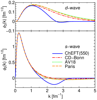
Figure 3: Deuteron $s$- and $d$-wave functions in momentum space described by various $NN$ interactions: ChEFT Epe05 , AV18 AV18 , CD-Bonn CDB , and Paris PARIS . The sign of the $d$-wave function is reversed. The normalization of these wave functions is $\int_{0}^{\infty}dk\>(\phi_{0}^{2}(k)+\phi_{2}^{2}(k))=1$.

Deuteron wave functions, the $s$ and $d$ components, are those of the N³LO ChEFT interactions with the cutoff of 550 MeV Epe05 . This scale of the wave functions and the 3BFs may not be soft enough to permit a perturbative treatment. Nevertheless, without strong short-range singularities, the resulting folding potential helps intuitively infer the $\Lambda$-deuteron interaction and therefore the possible role of the $\Lambda NN$ 3BFs to the hypertriton. It is noted that it is not appropriate to employ deuteron wave functions of other $NN$ interactions having strong short-range singularities together with the ChEFT 3BFs. For comparison, deuteron wave functions in momentum space are shown in Fig. 3 in which those of other $NN$ interactions, i.e., AV18 AV18 , CD-Bonn CDB , and Paris PARIS , are compared.

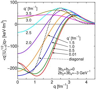
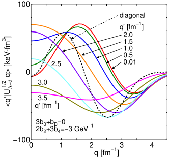
Figure 4: $\Lambda$-deuteron folding potential with $\ell_{\Lambda}=0$ from two-pion exchange $\Lambda NN$ interactions. The upper panel shows the contribution of the deuteron $s$-state pair. The lower panel shows the contribution of from the remaining pairs: $sd$, $ds$, and $dd$.

Calculated $s$-wave [$\ell_{\Lambda}^{\prime}=\ell_{\Lambda}=0$ in Eq. (23)] $\Lambda$-deuteron folding potential with $J_{t}=1/2$ from the leading-order $\Lambda NN$ interactions is presented in Fig. 4. The upper panel shows the contribution from the $s$-wave component of the deuteron wave function, in which $V_{TPE}^{(K=0,\ell_{a},\ell_{b})}$ participates. The lower panel presents the sum of the remaining contributions from the $s$-$d$, $d$-$s$, and $d$-$d$ pairs of the deuteron wave function. $V_{TPE}^{(K=2,\ell_{a},\ell_{b})}$ contributes in the $s$-$d$ and $d$-$s$ pairs. Both $V_{TPE}^{(K=0,\ell_{a},\ell_{b})}$ and $V_{TPE}^{(K=2,\ell_{a},\ell_{b})}$ contribute in the case of the $d$-$d$ pair. The potential with $J_{t}=3/2$ is identical to that with $J_{t}=1/2$ .

The employed parameters are taken from the estimation by Petshauer et al. Pet16 ; that is, $(3b_{0}+b_{D})=0$ and $(2b_{2}+3b_{4})=3.0\times 10^{-3}$ MeV^-1. In principle, parameters of the two-pion exchange 3BFs should be determined in fitting the two-body $\Lambda N$ interactions. However, the present experimental situation of the strangeness $S=-1$ sector does not allow such an investigation.

The calculated potential is weakly attractive, with a depth below about 200 keV. The experimental separation energy of the hypertriton is very small, $130\pm 50$ keV, though the actual value is still controversial. Therefore, its wave function extends and the $\Lambda NN$ 3BF contribution can be considered hindered. Still, the similar magnitude of the $\Lambda NN$ 3BF effect shown in Fig. 4 as the separation energy indicates that the effect may not be negligible in the hypertriton. Thus, it suggests that further study of the hypertriton in Faddeev formalism with incorporation of the 3BFs is necessary. The repulsive bump structure seen beyond $q\simeq 2.5$ fm implies that the scale of 550 MeV employed for the ChEFT description still has remnants of shorter-range singularities, which should be treated in a Faddeev framework.

V Summary

We have presented an expression of partial-wave decomposition of 3BFs concerning the relevant Jacobi momenta. The derivation essentially follows that of Hebeler et al. Heb15 , but the final formula differs in that it can systematically treat the higher-rank spin and angular-momentum tensor-product structure of 3BFs. Although the consideration is intended specifically for $\Lambda NN$ 3BFs and one set of the Jacobi momenta, the formula is general, as far as 3BFs are a function of the momentum transfer in each Jacobi momentum. Even if a regularization function is angle-dependent, the 3BFs can be expressed in the form of Eq. (2) and then the result of Eq. (22) is applicable.

As an application of the derived expression, the $\Lambda$-deuteron folding potential from NNLO $\Lambda NN$ 3BFs is evaluated. At the present stage, the construction of baryon-baryon interactions in the strangeness $S=-1$ sector in ChEFT is practiced up to the NLO level NLO13 ; HMN20 . Even at this low order, it is difficult to unambiguously determine coupling constants because of the lack of sufficient experimental data, and therefore a plausible assumption of the SU(3) symmetry has to be called for. In addition, there is no conclusive way to fix the parameters of the two-pion exchange $\Lambda NN$ 3BFs that are basically of the NNLO. This means that experimental and theoretical investigations are needed in the future. It is essentially important to quantitatively establish the contribution of $\Lambda NN$ 3BFs in hypernuclei, which is also relevant for the understanding of the appearance or absence of $\Lambda$ hyperons in neutron star matter MK18 ; GKW20 .

In particular, the investigation of the hypertriton is of fundamental importance. Before doing full Faddeev calculations for the hypertriton including $\Lambda NN$ 3BFs, it is worthwhile to estimate the possible role of the 3BFs for the hypertriton. The present folding potential calculation indicates the necessity of considering $\Lambda NN$ 3BFs in the theoretical study of the hypertriton because the quantitative estimation of their effects will influence the parametrization of $\Lambda N$ two-body interactions.

Acknowledgements. This work is supported by JSPS KAKENHI Grants No. JP19K03849 and No. JP22K03597.

Appendix A Tensor-product decomposition of $\Lambda NN$ three-body interactions

$V_{TPE}^{(K,\ell_{a},\ell_{b})}(p,q)$ in Eq. (2) for $K=0$, 1 and 2 in the case of the leftmost diagram of Fig. 1 are as follows:

$$V_{TPE}^{K=0,\ell_{a},\ell_{b}}(p,q)= (-1)^{\ell_{a}}\delta_{\ell_{a}\ell_{b}}\delta_{\ell_{a},even}\sqrt{\frac{\hat{\ell_{a}}}{3}}\frac{\{C_{0}m_{\pi}^{2}+C_{1}(-p^{2}+r_{NN}^{2}q^{2})\}(p^{2}-r_{NN}^{2}q^{2})}{2pr_{NN}q(p^{2}+r_{NN}^{2}q^{2}+m_{\pi}^{2})}Q_{\ell_{a}}(z_{pq}),$$ (25)

$$V_{TPE}^{K=1,\ell_{a},\ell_{b}}(p,q)= \delta_{\ell_{a}\ell_{b}}\delta_{\ell_{a},odd}\frac{\{C_{0}m_{\pi}^{2}+C_{1}(-p^{2}+r_{NN}^{2}q^{2})\}}{(p^{2}+r_{NN}^{2}q^{2}+m_{\pi}^{2})}\frac{1}{\hat{\ell_{a}}}\sqrt{\frac{\ell_{a}(\ell_{a}+1)}{6\hat{\ell_{a}}}}\{Q_{\ell_{a}+1}(z_{pq})-Q_{\ell_{a}-1}(z_{pq})\},$$ (26)

$$V_{TPE}^{K=2,\ell_{a},\ell_{b}}(p,q)= -\sqrt{\frac{2}{15}}\frac{\{C_{0}m_{\pi}^{2}+C_{1}(-p^{2}+r_{NN}^{2}q^{2})\}}{2pr_{NN}q(p^{2}+r_{NN}^{2}q^{2}+m_{\pi}^{2})}\sqrt{\hat{\ell_{a}}\hat{\ell_{b}}}(\ell_{a}0\ell_{b}0|20)\{p^{2}Q_{\ell_{b}}(z_{pq})-r_{NN}^{2}q^{2}Q_{\ell_{a}}(z_{pq})\},$$ (27)

where $C_{0}=-\frac{g_{A}^{2}}{3f_{0}^{4}}(3b_{0}+b_{D})$, $C_{1}=\frac{g_{A}^{2}}{3f_{0}^{4}}(2b_{2}+3b_{4})$, and $z_{pq}=\frac{p^{2}+r_{NN}^{2}q^{2}+m_{\pi}^{2}}{2pr_{NN}q}$. $Q_{\ell}$ is a Legendre polynomial of the second kind.

Appendix B Evaluation of $\Lambda$-deuteron folding potential from $\Lambda NN$ 3BFs

An explicit calculational procedure of the $\Lambda$-deuteron folding potential, given by Eq. (23), is provided. The abbreviated notation of Eq. (23) means

$$U_{\Lambda-d}^{J_{t}}(q_{1}^{\prime},q_{1})= \iint p_{1}^{\prime 2}dp_{1}^{\prime}p_{1}^{2}dp_{1}\langle[\Psi_{d}(\mbox{\boldmath$p$}_{1}^{\prime}),(\ell_{\Lambda}^{\prime}1/2)j_{\Lambda}]J_{t}|V_{TPE}^{\Lambda NN}|[\Psi_{d}(\mbox{\boldmath$p$}_{1}),(\ell_{\Lambda}1/2)j_{\Lambda}]J_{t}\rangle$$

$$= \sum_{\ell_{d}^{\prime}=0,2}\sum_{\ell_{d}=0,2}\iint p_{1}^{\prime 2}dp_{1}^{\prime}p_{1}^{2}dp_{1}\frac{1}{p_{1}^{\prime}}\phi_{\ell_{d}}(p_{1}^{\prime})\frac{1}{p_{1}}\phi_{\ell_{d}}(p_{1})\langle[[Y_{\ell_{d}^{\prime}}(\hat{\mbox{\boldmath$p$}_{1}^{\prime}})\times\chi_{d}^{1}]^{1}\times[Y_{\ell_{\Lambda}^{\prime}}(\hat{\mbox{\boldmath$q$}_{1}^{\prime}})\times\chi_{\Lambda}^{1/2}]^{j_{\Lambda}}]_{M_{t}}^{J_{t}}|$$

$$\times V_{TPE}^{\Lambda NN}|[[Y_{\ell_{d}}(\hat{\mbox{\boldmath$p$}_{1}})\times\chi_{d}^{1}]^{1}\times[Y_{\ell_{\Lambda}}(\hat{\mbox{\boldmath$q$}_{1}})\times\chi_{\Lambda}^{1/2}]^{j_{\Lambda}}]_{M_{t}}^{J_{t}}\rangle,$$ (28)

where $\chi_{d}^{1}$ and $\chi_{\Lambda}^{1/2}$ denote spin functions for the deuteron and the $\Lambda$ hyperon, respectively. The isospin degrees of freedom are not explicitly shown. Because the isospin of the $\Lambda$ hyperon is 0 and that of the deuteron is 0, the matrix element of the isospin operator $(\mbox{\boldmath$\tau$}_{2}\cdot\mbox{\boldmath$\tau$}_{3})$ in Eq. (2) becomes $-3$. Substituting $V_{TPE}^{\Lambda NN}$ of Eq. (2), the following angular-momentum recoupling is carried out:

$$\langle[[Y_{\ell_{d}^{\prime}}(\hat{\mbox{\boldmath$p$}_{1}^{\prime}})\times\chi_{d}^{1}]^{1}\times[Y_{\ell_{\Lambda}^{\prime}}(\hat{\mbox{\boldmath$q$}_{1}^{\prime}})\times\chi_{\Lambda}^{1/2}]^{j_{\Lambda}}]_{M_{t}}^{J_{t}}|V_{TPE}^{(K,\ell_{a},\ell_{b})}(p,q)[[Y_{\ell_{a}}(\hat{\mbox{\boldmath$p$}})\times Y_{\ell_{b}}(\hat{\mbox{\boldmath$q$}})]^{K}\times[\mbox{\boldmath$\sigma$}_{2}\times\mbox{\boldmath$\sigma$}_{3}]^{K}]_{0}^{0}$$

$$\times|[[Y_{\ell_{d}}(\hat{\mbox{\boldmath$p$}_{1}})\times\chi_{d}^{1}]^{1}\times[Y_{\ell_{\Lambda}}(\hat{\mbox{\boldmath$q$}_{1}})\times\chi_{\Lambda}^{1/2}]^{j_{\Lambda}}]_{M_{t}}^{J_{t}}\rangle$$

$$= \sum_{L^{\prime}L}\sum_{S^{\prime}S}3\hat{j_{\Lambda}}\sqrt{\hat{L^{\prime}}\hat{S^{\prime}}\hat{L}\hat{S}}\begin{Bmatrix}\ell_{d}^{\prime}&\ell_{\Lambda^{\prime}}&L^{\prime}\\ 1&1/2&S^{\prime}\\ 1&j_{\Lambda^{\prime}}&J_{t}\end{Bmatrix}\begin{Bmatrix}\ell_{d}&\ell_{\Lambda}&L\\ 1&1/2&S\\ 1&j_{\Lambda^{\prime}}&J_{t}\end{Bmatrix}\langle[[Y_{\ell_{d}^{\prime}}(\hat{\mbox{\boldmath$p$}_{1}^{\prime}})\times Y_{\ell_{\Lambda}^{\prime}}(\hat{\mbox{\boldmath$q$}_{1}^{\prime}})]^{L^{\prime}}\times[\chi_{d}^{1}\times\chi_{\Lambda}^{1/2}]^{S^{\prime}}]_{M_{t}}^{J_{t}}|$$

$$\times V_{TPE}^{(K,\ell_{a},\ell_{b})}(p,q)[[Y_{\ell_{a}}(\hat{\mbox{\boldmath$p$}})\times Y_{\ell_{b}}(\hat{\mbox{\boldmath$q$}})]^{K}\times[\mbox{\boldmath$\sigma$}_{2}\times\mbox{\boldmath$\sigma$}_{3}]^{K}]_{0}^{0}|[[Y_{\ell_{d}}(\hat{\mbox{\boldmath$p$}_{1}})\times Y_{\ell_{\Lambda}}(\hat{\mbox{\boldmath$q$}_{1}})]^{L}\times[\chi_{d}^{1}\times\chi_{\Lambda}^{1/2}]^{S}]_{M_{t}}^{J_{t}}\rangle$$

$$= \sum_{L^{\prime}L}\sum_{S^{\prime}S}3\hat{j_{\Lambda}}\sqrt{\hat{L^{\prime}}\hat{S^{\prime}}\hat{L}\hat{S}}\begin{Bmatrix}\ell_{d}^{\prime}&\ell_{\Lambda^{\prime}}&L^{\prime}\\ 1&1/2&S^{\prime}\\ 1&j_{\Lambda^{\prime}}&J_{t}\end{Bmatrix}\begin{Bmatrix}\ell_{d}&\ell_{\Lambda}&L\\ 1&1/2&S\\ 1&j_{\Lambda^{\prime}}&J_{t}\end{Bmatrix}\sqrt{\hat{J_{t}}\hat{L^{\prime}}\hat{S^{\prime}}}\begin{Bmatrix}J_{t}&J_{t}&0\\ L^{\prime}&L&K\\ S^{\prime}&S&K\end{Bmatrix}$$

$$\times\langle[Y_{\ell_{d}^{\prime}}(\hat{\mbox{\boldmath$p$}_{1}^{\prime}})\times Y_{\ell_{\Lambda}^{\prime}}(\hat{\mbox{\boldmath$q$}_{1}^{\prime}})]^{L^{\prime}}||V_{TPE}^{(K,\ell_{a},\ell_{b})}(p,q)[Y_{\ell_{a}}(\hat{\mbox{\boldmath$p$}})\times Y_{\ell_{b}}(\hat{\mbox{\boldmath$q$}})]^{K}||[Y_{\ell_{d}}(\hat{\mbox{\boldmath$p$}_{1}})\times Y_{\ell_{\Lambda}}(\hat{\mbox{\boldmath$q$}_{1}})]^{L}\rangle_{pwe}$$

$$\times 18\sqrt{\hat{S}\hat{K}}(-1)^{K+3/2+S}\begin{Bmatrix}S^{\prime}&S&K\\ 1&1&1/2\end{Bmatrix}\begin{Bmatrix}1&1&K\\ 1/2&1/2&1\\ 1/2&1/2&1\end{Bmatrix},$$ (29)

where $\mbox{\boldmath$p$}=\mbox{\boldmath$p$}_{1}^{\prime}-\mbox{\boldmath$p$}_{1}$ and $\mbox{\boldmath$q$}=\mbox{\boldmath$q$}_{1}^{\prime}-\mbox{\boldmath$q$}_{1}$. Then, Eq. (22) is applied in this expression. The result does not depend on $M_{t}$. Numerical results of the case of $\ell_{d}^{\prime}=\ell_{d}=0$ are presented in Sec. IV.

References

• (1) H. WitaΕ‚a, W. GlΓΆckle, D. HΓΌber, J. Golak, and H. Kamada, ”Cross Section Minima in Elastic Nd Scattering: Possible Evidence for Three-Nucleon Force Effects,” Phys. Rev. Lett. 81, 1183 (1998).
• (2) K. Sekiguchi, H. Sakai, H. WitaΕ‚a, W. GlΓΆckle, J. Golak, M. Hatano et al., ”Complete set of precise deuteron analyzing powers at intermediate energies: Comparison with modern nuclear force predictions,” Phys. Rev. C 65, 034003 (2002).
• (3) S. C. Pieper, V. R. Pandharipande, R. B. Wiringa, and J. Carlson, ”Realistic models of pion-exchange three-nucleon interactions,” Phys. Rev. C 64, 014001 (2001).
• (4) A. Akmal, V. R. Pandharipande, and D. G. Ravenhall, ”Equation of state of nucleon matter and neutron star structure,” Phys. Rev. C 58, 1804 (1998).
• (5) M. Baldo and G. F. Burgio, ”Properties of the nuclear medium,” Rep. Prog. Phys. 75, 026301 (2012).
• (6) E. Epelbaum, H.-W. Hammer, and U.-G. Meißner, ”Modern theory of nuclear force,” Rev. Mod. Phys. 81, 1773 (2009).
• (7) R. Machleidt and D. R. Entem, β€œChiral effective field theory and nuclear forces,” Phys. Rep. 503, 1 (2011).
• (8) K. Hebeler, H. Krebs, E. Epelbaum, J. Golak, and R. SkibiΕ„ski, ”Efficient calculation of chiral three-nucleon forces up to N3LO for ab initio studies,” Phys. Rev. C 91, 044001 (2015).
• (9) S. Petschauer, N. Kaiser, J. Haidenbauer, U.-G. Meißner, and W. Weise, ”Leading three-baryon forces from SU(3) chiral effective field theory,” Phys. Rev. C 93, 014001 (2016).
• (10) W. GlΓΆckle, H. WitaΕ‚a, D. HΓΌber, H. Kamada, J. Golak, β€œThe three-nucleon continuum: Achievements, challenges and applications”, Phys. Rep. 274, 107 (1996).
• (11) K. Miyagawa, H. Kamada, W. GlΓΆckle, V. Stoks, ”Properties of the bound $\Lambda$($\Sigma$)NN system and hyperon-nucleon interactions”, Phys. Rev. C 51, 2905 (1995).
• (12) J. Haidenbauer, U.-G. Meißner, and A. Nogga, ”Hyperon-nucleon interaction within chiral effective field theory revisited”, Eur. Phys. J. A 56, 91 (2020).
• (13) The STAR Collaboration, ”Measurement of the mass difference and the binding energy of the hypertriton and antihypertriton”, Nature Phys. 16, 409 (2020).
• (14) E. Epelbaum, W. GlΓΆckle, and U.-G. Meißner, ”The two-nucleon system at next-to-next-to-next-to-leading order,” Nucl. Phys. A 747, 362 (2005).
• (15) R. B. Wiringa, V. G. J. Stoks, and R. Schiavilla, ”Accurate nucleon-nucleon potential with charge-independence breaking,” Phys. Rev. C 51, 38 (1995).
• (16) R. Machleidt, ”High-precision, charge-dependent Bonn nucleon-nucleon potential,” Phys. Rev. C 63, 024001 (2001).
• (17) M. Lacombe, B. Loiseau, R. Vinh Mau, J. CΓ΄tΓ©, P. PirΓ©s, and R. de Tourreil, ”Parametrization of the deuteron wave function of the Paris potential,” Phys. Lete. 101B, 139 (1981).
• (18) J. Haidenbauer, S. Petschauer, N. Kaiser, U.-G. Meißner, A. Nogga, and W. Weise, ”Hyperon-nucleon interaction at next-to-leading order in chiral effective field theory,” Nucl. Phys. A 915, 24 (2013)
• (19) M. Kohno, ”Single-particle potential of the hyperon in nuclear matter with chiral effective field theory NLO interactions including effects of YNN three-baryon interactions,” Phys. Rev. C 97, 035206 (2018).
• (20) D. Gerstung, N. Kaiser, and W. Weise, ”Hyperon-nucleon three-body forces and strangeness in neutron stars,” Eur. Phys. J. A 56, 175 (2020).