High-temperature self-energy corrections to x-ray absorption spectra

Abstract

Effects of finite-temperature quasiparticle self-energy corrections to x-ray absorption spectra are investigated within the finite-temperature quasiparticle local density GW approximation up to temperatures $T$ of order the Fermi temperature. To facilitate the calculations, we parametrize the quasiparticle self-energy using low-order polynomial fits. We show that temperature-driven decrease in the electron lifetime substantially broadens the spectra in the near-edge region with increasing $T$. However, the quasiparticle shift is most strongly modified near the onset of plasmon excitations.

I Introduction

Calculations of x-ray absorption spectra (XAS) at finite temperature (FT) have been carried out routinely in recent years. These studies range from relatively low temperatures up to a few hundred K (LT), to the warm dense matter (WDM) regime at high-temperatures (HT), where $T$ is of order the Fermi temperature $T_{F}$ [1, 2, 3, 4, 5, 6, 7, 8, 9]. A standard FT approach is to apply Fermi’s golden rule with initial and final states calculated using conventional density functional theory (DFT) and Fermi occupation factors. Since DFT is a ground state theory, FT quasiparticle corrections to DFT are essential for HT excited state calculations [10, 11]. However, even at extreme temperatures, e.g., many thousands of K, self-consistent field calculations of the core-hole state have sometimes been done with ground state exchange-correlation functionals $\varepsilon_{xc}[\rho]$ [2, 12, 13, 8]. This ground-state approximation can be unreliable in that its validity depends strongly on the system state and its properties. Some properties are only weakly sensitive to the temperature dependence of exchange and correlation, at least for low temperatures well below the WDM regime. Others, such as the electrical conductivity and x-ray absorption spectra (XAS), are strongly temperature dependent [14, 15]. Nevertheless, the use of temperature-dependent free-energy exchange-correlation functionals $f_{xc}[\rho,T]$ [16, 17, 18, 19, 20, 21, 15] alone ignores effects like inelastic losses. For example, the electron inelastic scattering effect, which results in an energy-dependent broadening, is often included via a post-processing step by convolution of the absorption cross-section using an empirical model (e.g. Seah-Dench formalism [22, 23]), or the imaginary part of the self-energy [24]. However, the finite temperature dependence of the energy-dependent broadening is typically neglected.

Another common approach for XAS calculations has been the use of the real-space multiple scattering (RSMS) method, which is also referred to as the real-space Green’s function (RSGF) method [25]. This approach is the real-space analog of the Korringa-Kohn-Rostoker (KKR) approach [26, 27, 28, 29, 30]. The method treats excited quasiparticle states via an energy-dependent self-energy, and also takes into account the dynamic response of the system to the suddenly created core-hole. The self-energy can be viewed as an energy-dependent, non-local analog of the exchange-correlation potential in DFT [31]. The FT generalization of the self-energy can be done formally via the Matsubara formalism. For example, Benedict et al. used the approach to investigate the effect of $T$ on the spectral function in jellium and aluminum, e.g., on optical properties of solid-density Al. Alternatively, as discussed by Kas et al. [33], the FT self-energy can be calculated using a generalization of the Migdal approximation [34], analogous to the FT $GW$ approximation of Hedin [35].

Our main goal in this work is to discuss the effects of the FT GW self-energy on XAS, an approach that heretofore has not been explored in detail [36]. In particular, to facilitate the calculations we introduce a parametrization of the quasiparticle FT GW self-energy within the $G_{0}W_{0}$ scheme [37]. As illustrations we apply the approach to the XAS for two systems with $T$ up to 10 eV (i.e. $T$ of order $10^{5}$ K). Our calculations demonstrate that thermal broadening due to the imaginary part of the self-energy are significant above $T\approx 1$ eV. Although lattice vibrations also are strongly temperature dependent, that behavior is dependent on the lattice temperature $T_{l}$ which can differ from the electronic temperature $T$ in non-equilibrium states, as discussed in a previous work [36].

The remainder of the paper is organized as follows. Section II. provides an brief overview of the real-space Green’s function approach to XAS and its dependence on the self-energy $\Sigma$. In Section III, we highlight the FT corrections to XAS with a few examples and in Section IV, we present a brief summary and conclusions. Throughout we use Hartree atomic units $q_{e}=\hbar=m=1$, with $q_{e}=e$ the electron charge. Thus energies are in Hartree and distances in Bohr, unless otherwise noted. For temperature we use either K or eV, with 1 eV $\approx$ 11,604 K. Electron densities are expressed in Wigner-Seitz radii $r_{s}=(3/4\pi\rho)^{1/3}$.

II Theory Summary

II.1 Finite-temperature X-ray Absorption

Formally the zero temperature X-ray absorption cross section is defined via Fermi’s golden rule as

$$\sigma(\omega)=4\pi^{2}\frac{\omega}{c}\sum_{i,f}|\langle\Psi_{i}|\hat{\xi}\cdot\mathbf{R}|\Psi_{f}\rangle|^{2}\delta_{\Gamma}(\omega+E_{i}-E_{f}),$$ (1)

where $|\Psi_{i}\rangle$ and $|\Psi_{f}\rangle$ are the many-body initial and final states, $\hat{\xi}$ is the polarization of the incident photon, and $\mathbf{R}$ is the many-body position operator. Then within the single-particle (quasiparticle) approximation with dipole interactions and the sudden approximation, the zero temperature XAS becomes

$$\sigma_{s}(\omega)=4\pi^{2}\frac{\omega}{c}\sum_{i,f}|\langle i|{d}|f\rangle|^{2}\delta_{\Gamma}(\omega+\varepsilon_{i}-\varepsilon_{f}),$$ (2)

where $\varepsilon_{i}$ and $\varepsilon_{f}$ are the energies of the quasiparticle initial $|i\rangle$ and final $|f\rangle$ levels and many-body shake-up factors $S_{0}^{2}\approx 1$ are ignored. The $\delta_{\Gamma}$ factor denotes a Lorentzian of width $\Gamma$ which includes both quasiparticle and core-hole lifetime broadening. Here, the transition operator ${d=\hat{\xi}\cdot{\bf r}}=$ is the single-particle electric dipole operator. The one-particle states $|i\rangle$ and $|f\rangle$ can be obtained from Hartree-Fock theory or Kohn-Sham DFT. For the treatment via DFT, see e.g., Refs. 38, 39, 40.

For x-ray absorption, the number of final states $|f\rangle$ required to compute the dipole matrix element has an impact on the computational efficiency of evaluating Eq. (2). The present work uses the RSMS approach to alleviate this bottleneck. In RSMS, we replace the summation over the final states $|f\rangle$ with the retarded single-electron Green’s function $G(\omega)$ in a basis of local site-angular momentum states $|Lj\rangle$ [25],

$$G^{jj^{\prime}}_{LL^{\prime}}(\omega)=\sum_{f}\frac{\langle Lj|f\rangle\langle f|L^{\prime}j^{\prime}\rangle}{\omega-\varepsilon_{f}+i\eta}\;.$$ (3)

In this expression, $j$ is the index of a given site $\mathbf{R}_{j}$ and $L=(l,m)$ are the angular momentum quantum numbers. The initial states $|i\rangle$ are calculated with the ground state Hamiltonian $H=p^{2}/2+v(r)$ while the final states $|f\rangle$ are described by the quasiparticle Hamiltonian $H^{\prime}=p^{2}/2+v_{f}(r)+\Sigma(r,E)$, where $v(r)$ is the self-consistent one-electron Hartree potential, $v_{f}$ is the final state one electron Hartree potential in the presence of a screened core hole, and $\Sigma$ is the dynamically screened quasiparticle self-energy discussed in detail below.

The imaginary part of the quasiparticle self-energy $\Sigma$ accounts for the mean free path of the photoelectron. Within the quasiparticle local density approximation (QPLDA) [41], the self-energy is given by [42]

$$\Sigma(\textbf{r},E,T=0) = v^{LDA}_{xc}(\rho(\textbf{r}))+\Sigma_{GW}(\rho(\textbf{r}),E,T=0)$$ (4)

$$-\Sigma_{GW}(\rho(\textbf{r}),E_{F},T=0)\;.$$

Here $\Sigma_{GW}$ is the $GW$ self-energy calculated at the $G_{0}W_{0}$ level of refinement, that is, without self-consistent iteration of $G$ or $W$ [35]. For simplicity from here onward, we drop the spatial dependence r.

For the FT generalization, we replace the $T=0$ $GW$ self-energy with the finite-temperature $GW$ self-energy, $\Sigma_{GW}(T)$, and introduce $T$-dependent Fermi occupation numbers, $f(\varepsilon)=1/[\exp{\{\beta(\varepsilon-\mu)\}}+1]$ for the initial and final states in Eq. (2). In addition, the ground state exchange-correlation potential $v^{LDA}_{xc}$ is replaced by its FT generalization $v^{LDA}_{xc}(T)$. Thus, the finite-temperature QPLDA self-energy is

$$\Sigma(E,T) = v^{LDA}_{xc}(\rho,T)+\Sigma_{GW}(\rho,E,T)$$ (5)

$$-\textnormal{Re}\ [\Sigma_{GW}(\rho,\mu_{T},T)]$$

Lastly, by using $G^{jj^{\prime}}_{LL^{\prime}}(\omega)$ in Eq. (2) in place of the sum over final states $|f\rangle$, the FT quasiparticle cross section can be re-expressed as:[43]

$$\sigma_{qp}(\omega) = -4\pi^{2}\frac{\omega}{c}{\textnormal{Im}}\sum_{iLL^{\prime}}\langle i|\hat{d}G^{00}_{LL^{\prime}}(\omega+\varepsilon_{i})\hat{d}^{\dagger}|i\rangle$$ (6)

$$\times f(\varepsilon_{i})\big{[}1-f(\omega+\varepsilon_{i})\big{]},$$

Here, we denote the absorbing atom by the index 0.

II.2 Finite-temperature Self-energy $\Sigma$

The finite-$T$ quasiparticle electron self-energy within the $GW$ approximation is defined formally [34, 44] by the expression

$$\Sigma^{M}_{GW}({\mathbf{k}},i\omega_{m}) = -\frac{1}{\beta}\int\frac{d^{3}{\mathbf{q}}}{(2\pi)^{3}}\sum_{n=-\infty}^{\infty}G_{0}^{M}({\mathbf{k}}-{\mathbf{q}},i\omega_{m}-i\nu_{n})$$ (7)

$$\times W^{M}({\mathbf{q}},i\nu_{n})\;.$$

Here $G_{0}^{M}$ is the one-electron Matsubara Green’s function, $W^{M}=\epsilon^{-1}v$ is the screened Coulomb interaction, and $\omega_{m}=2(m+1)\pi k_{B}T$, $\nu_{n}=2n\pi k_{B}T$ are the Matsubara frequencies, where $\epsilon$ is the dielectric function and $v$ is the bare Coulomb potential. The screened interaction $W^{M}$ can be expressed in terms of its spectral representation as

$$W^{M}({\mathbf{q}},i\nu_{n}) = v({\mathbf{q}})+\int_{-\infty}^{\infty}d\omega^{\prime}\frac{D({\mathbf{q}},\omega^{\prime})}{i\nu_{n}-\omega^{\prime}+i\eta\,{\textnormal{sgn}}(\omega^{\prime})}$$ (8)

where $v({\mathbf{q}})=4\pi/q^{2}$ is the bare Coulomb potential in Fourier representation, and $D({\mathbf{q}},\omega)=(1/\pi)|{\textnormal{Im}}\,W^{M}_{c}({\mathbf{q}},\omega)|\,{\textnormal{sgn}}(\omega)$ is the anti-symmetric (in frequency) bosonic excitation spectrum. $W^{M}_{c}=W^{M}-v$ is the correlation part of the screened interaction.

Our choice of the electron gas dielectric function reflects a balance between the level of physics included and computational feasibility. Thus for simplicity, we use the random phase approximation (RPA), which is analogous to the FT generalization of the Lindhard function [45],

$$\epsilon({\mathbf{q}},\omega,T) = 1+2v({\mathbf{q}})\int\frac{d^{3}{\mathbf{k}}}{(2\pi)^{3}}\frac{f(\varepsilon_{{\mathbf{k}}-{\mathbf{q}}})-f(\varepsilon)}{\omega-\varepsilon_{{\mathbf{k}}-{\mathbf{q}}}+\varepsilon_{\mathbf{k}}+i\eta},$$ (9)

where $f(\varepsilon)=1/[\exp{\{\beta(\varepsilon-\mu)\}}+1]$ is the Fermi-Dirac occupation factor, and $\mu=\mu(T)$ is the chemical potential. The real part of $\epsilon({\mathbf{q}},\omega,T)$ is obtained from the imaginary part via a Kramers-Kronig transform. From an analytic continuation to the real-$\omega$ axis, the FT GW retarded self-energy $\Sigma_{GW}$ is given by the Migdal approximation [34]

$$\Sigma_{GW}({\mathbf{k}},\omega,T)=\Sigma_{X}({\mathbf{k}},\omega,T)+\int_{0}^{\infty}d\omega^{\prime}\int\frac{d^{3}{\mathbf{q}}}{(2\pi)^{3}}D({\mathbf{q}},\omega^{\prime})$$ (10)

$$\times \bigg{[}\frac{f(\varepsilon_{{\mathbf{k}}-{\mathbf{q}}})+N(\omega^{\prime})}{\omega+\omega^{\prime}-\varepsilon_{{\mathbf{k}}-{\mathbf{q}}}+i\eta}+\frac{1-f(\varepsilon_{{\mathbf{k}}-{\mathbf{q}}})+N(\omega^{\prime})}{\omega-\omega^{\prime}-\varepsilon_{{\mathbf{k}}-{\mathbf{q}}}+i\eta}\bigg{]},$$

where $\Sigma_{X}({\mathbf{k}},\omega,T)=\int[d^{3}{\mathbf{q}}/(2\pi)^{3}]f(\varepsilon_{{\mathbf{k}}-{\mathbf{q}}})v_{\mathbf{q}}$ is the exchange part of self-energy and $N(\omega)=1/[\exp\{\beta\omega\}-1]$ is the Bose factor. The poles of the Green’s function $G^{M}$ contribute to the Fermi occupations whereas the poles of the screened interaction $W^{M}$ contribute to the Bose factor.

Calculations of the imaginary part of $\Sigma_{GW}({\mathbf{k}},\omega,T)$ involves a singe integral over the magnitude of ${\mathbf{q}}$ but to obtained the real part we need to perform a Kramers-Kronig transform resulting in a double integral. In typical RSGF XAS calculations [46], tens of thousands of self-energy evaluations are required. Thus that calculation of quasiparticle self-energy $\Sigma_{GW}(k,k^{2}/2,T)$ immediately becomes a computational bottleneck. To circumvent that difficulty, we model $\Sigma_{GW}(k,k^{2}/2,T)$ via low-order polynomial fits to numerical calculation of $\Sigma_{GW}$ based on Eq. (10), on a grid up to $T=2T_{F}$, where $T_{F}=E_{F}/k_{B}$. The form of the fitting functions is described in detail in the Appendices. A comparison between the QPLDA $\Sigma_{GW}$ and the fits is shown in Fig. 1 for the homogeneous electron gas. For simplicity, we approximate the self-energy for levels $k<k_{F}$ with $v_{xc}(T)$ independent of $k$.

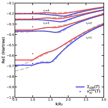
Figure 1: The real part of the $\Sigma_{GW}$ (dashed) and our parametrization (solid) for various densities: $r_{s}$ = 1.0, 2.0, 3.0, 4.0 at $T/T_{F}$ = 0.01 (blue) and 1.0 (red). For reference the LDA-$v_{xc}$(T) [20] values are denoted as dots at $k_{F}$.

III Results and Discussion

In this section, we present our results showing effects of the use of the FT $\Sigma_{GW}(T>0)$ instead of the zero $T$ values $\Sigma_{GW}(T=0)$. Note that $\Sigma_{GW}(T=0)$ depends implicitly on the electronic temperature $T$ through the self-consistent electron density at that temperature. The FT SCF calculations are carried out using an extension of the original RSMS code, which is now implemented in FEFF10 [46, 47]. For the FT exchange correlation-potential, we use the KSDT tabulation $v^{LDA}_{xc}(T)$ [20, 48] for both calculations. In the FEFF10 calculations, we compute the atomic part with the ground state exchange potential, whereas we use $\Sigma_{GW}(T)$ for the fine structure.

As noted in Ref. [2, 8], corrections to the core energy levels are needed for $T\gtrsim 1$ eV. We compute the core level shifts using the all-electron full-potential linearized plane wave code FLEUR [49, 50, 51]. Within these calculations, we ignore the explicit temperature dependence in the LDA exchange correlation functional [52]. As a side note, FLEUR uses non-overlapping muffin-tin potentials whereas FEFF uses overlapping muffin-tin potentials.

In the RSMS formalism, the decomposition of the Green’s function $G$ into a central atom $G^{c}$ contribution and a multiple-scattering $G^{sc}$ contribution allows us to describe the XAS in terms of the atomic background $\sigma_{0}$ and the oscillatory fine structure $\chi$, i.e., $\sigma=\sigma_{0}(1+\chi)$. For many XANES calculations, it is found that the atomic background matches the experimental results better when calculated without the self-energy corrections due to the overestimation of the exchange within the muffin-tin (MT) potential approximation [53]. Fig. 2 shows the effect of using the ground-state potential versus the use of $\Sigma_{GW}(T)$ for the atomic background. The pre-edge is dominated by the atomic background and thus is sensitive to the choice of exchange potential. The pre-edge amplitude is reduced by $\approx 28\%$ due to the temperature correction of $\Sigma_{GW}(T)$. More pump-probe experimental XAS measurements for $T\approx 10$ eV are required to validate the FT self-energy effect for the atomic background. Nonetheless, the FT self-energy corrections are important for the description of HT fine-structure.

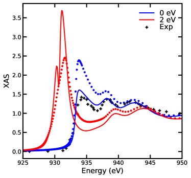
Figure 2: $\textnormal{L}_{3}$-edge XAS for Cu (lattice constant $a=3.61$ Å[54]) at electronic temperature $T=0$ eV and 2 eV. The solid curves denote the absorption with ground state atomic background while the dots represent the absorption with $\Sigma_{GW}(T>0)$ self-energy atomic background. The experimental measurement at ambient condition is shown as black cross.[55]

As a first example, we consider the FT K-edge x-ray absorption near-edge spectrum (XANES) for aluminum (fcc Al, lattice constant $a=4.05$ Å[54]). Al is a prototypical nearly-free electron system in the sense that the electronic density of states (DOS) in the conduction band has a nearly square root like dispersion at the bottom of the band. Fig. 3 shows the comparison of the Al K-edge spectrum at different temperatures including or excluding explicit electronic T-dependent effects in the self-energy, namely, using $\Sigma_{GW}(T=0)$ or $\Sigma_{GW}(T>0)$. When restricting the temperature T solely to that which is introduced through the density ($\Sigma_{GW}(T=0)$ case), we observe the broadening of the edge and no shift in the edge position. The shift in the core levels compensates for the shift in the valence density. On the other hand, for $T$ up to about 1 eV, the finite temperature self-energy correction is negligible, and the temperature-independent electron self-energy model is a good approximation. However, as temperature grows to order $\approx$ 10 eV, the fine structures are smoothed by the large broadening ($\approx$ 3 eV) associated with shortened electronic excitation lifetime. The shift in quasiparticle shift due to the finite temperature self-energy correction is small for the near-edge region, and only becomes significant between 10 eV and 20 eV above the chemical potential.

As a further illustration of the explicit $T$-dependence of the FT quasiparticle self-energy, we compute the quasiparticle energy correction $\Delta_{k}=\varepsilon_{qp}-\varepsilon_{k}$. Here, the quasiparticle energy $\varepsilon_{qp}$ is the solution to $\varepsilon_{qp}(k^{\prime})=\varepsilon_{k}+\Sigma_{GW}(k^{\prime},\varepsilon_{qp}(k^{\prime}))$ and $k=\sqrt{2(E-\mu)}$ is the photoelectron wavenumber. We compare the real part of $\Delta$ in Fig. 4 and imaginary part in Fig. 5 for different self-energies at the interstitial density: $\Sigma_{GW}(T=0)$ and $\Sigma_{GW}(T>0)$. Note that the real part of $\Delta$ shows a strong temperature dependence between 5 eV and 20 eV near the plasmon onset. For the imaginary part of $\Delta$, the broadening effect becomes important above $T$ = 1 eV.

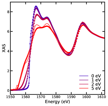
Figure 3: K-edge XAS for fcc aluminum ($a=4.05$ Å) using different self-energies: $T$-independent GW self-energy $\Sigma_{GW}(T=0)$ (solid curves) and $T$-dependent GW self-energy $\Sigma_{GW}(T>0)$ (dots).

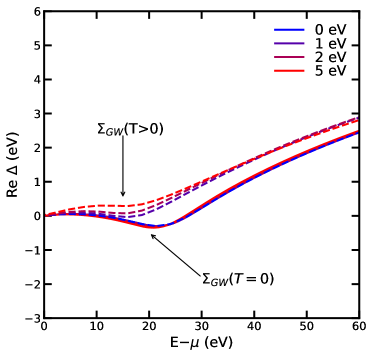
Figure 4: The quasiparticle corrections Re $\Delta_{k}$ for aluminum at temperatures $T=0,1,2$ and $5$ eV. The calculations used KSDT $v_{xc}(T)$ and different self-energies: $\Sigma_{GW}(T=0)$ (solid), and $\Sigma_{GW}(T>0)$ (dashed).

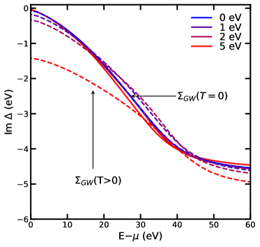
Figure 5: The quasiparticle corrections Im $\Delta_{k}$ for aluminum at temperatures $T=0,1,2$ and $5$ eV. The calculations used KSDT $v_{xc}(T)$ and different self-energies: $\Sigma_{GW}(T=0)$ (solid), and $\Sigma_{GW}(T>0)$ (dashed).

As a second example, we present results for a noble transition metal (fcc copper, lattice constant $a=3.61$ Å[54]) for which the $d$-bands are essentially full. Unlike the K-edge, the L-edge probes the highly-localized $d$-bands of Cu near the chemical potential. At high temperatures, the pre-edge peak increases in amplitude due to the decreasing $d$-state occupation [8, 36]. Fig. 6 shows the $\textnormal{L}_{3,2}$-edge XAS up to $T=5$ eV. The temperature dependence of $\textnormal{Im}\ \Sigma_{GW}(T)$ results in changes to pre-edge peaks at $T\gtrapprox 2$ eV. Consequently, the estimation of temperature based on the pre-edge area method or direct spectrum fitting will deviate more from the $\Sigma_{GW}(T=0)$ model as temperature increases.

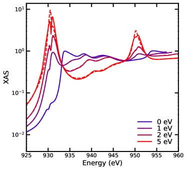
Figure 6: $\textnormal{L}_{3,2}$-edge XAS for Cu ($a=3.61$ Å) finite electronic temperature $T=0,1,2$ and $5$ eV, where the structure reflects that of the unfilled $d$-bands. The solid curves denote the $\Sigma_{GW}(T=0)$ self-energy results while the dashes represent the $\Sigma_{GW}(T>0)$ self-energy results.

IV Summary, Conclusions, and Outlook

Our parametrization of the FT GW electron self-energy enables efficient calculations of XAS at finite $T$, from LT of a few hundred K, up to the WDM regime with $T$ at least 10 eV. Our strategy uses the QPLDA $G_{0}W_{0}$ level of refinement for the self-energy, with the RPA dielectric function in conjunction with the KSDT finite-$T$ LDA exchange-correlation functional. Specifically, the FT self-energy for a system is approximated using the uniform electron gas with density equal to that of the local density. This is a significant simplification, as direct calculations using the exact loss function of the system for the entire energy range of typical XAS experiments would be computationally formidable. A finite-temperature SCF procedure for the XAS calculations is carried out in the complex energy plane in terms of the FT one-electron Green’s function. The procedure includes the FT exchange-correlation potential, approximated here by the KSDT parametrization. Important FT XAS effects include the smearing of the absorption edge and the presence of peaks in the spectrum below the $T=0$ K Fermi energy. The FT exchange-correlation potential has only a small effect on XAS at low temperatures $T\ll T_{F}$ compared to the effect of Fermi smearing. The FT self-energy is also important for XAS, accounting for both temperature dependent shifts and final-state broadening. To illustrate its efficacy, the approach was applied to calculations of XANES for crystalline Al and Cu at normal density. Above $T>1$ eV, the fine structures experience substantial broadening in the K-edges, corresponding to a reduction of the quasiparticle lifetime with increasing $T$.

Going forward, a computationally efficient approximation beyond the uniform electron gas dielectric function would be to use a many-pole model [56, 57], which is an extension of the Hedin-Lundqvist single plasmon-pole model [58, 59]. Ab-initio dielectric functions also can be obtained from modern electronic structure codes. Such a finite-temperature generalization of the many-pole model is currently under development.

Appendix A Model for $\textnormal{Re}\ \Sigma_{GW}$

The real part of the finite temperature GW self-energy, $\textnormal{Re}\ \Sigma_{GW}(T)$, is parametrized using low-order polynomials. The parametric variables are the Wigner-Seitz radius $r_{s}$, reduced momentum $x=k/k_{F}$ and reduced temperature $t=T/T_{F}$. Below the variable $X$ represents the array denoted $X=(r_{s},x,t)$.

$$\frac{\textnormal{Re}\ \Sigma_{GW}(X)}{E_{F}} = \begin{cases}\alpha_{0}(t)+\alpha_{1}(t)\beta_{1}(r_{s})x\\ +\alpha_{2}(t)\beta_{2}(r_{s})x^{3/2}\\ +\alpha_{3}(t)\beta_{3}(r_{s})x^{2}\\ +\alpha_{4}(t)\beta_{4}(r_{s})x^{5/2},x<\kappa(r_{s},t)\\ \\ \tilde{\alpha}_{1}(t)\tilde{\beta}_{1}(t)/x^{-1}\\ +\tilde{\alpha}_{2}(t)\tilde{\beta}_{2}(t)/x^{-2}\\ +\tilde{\alpha}_{3}(t)\tilde{\beta}_{3}(t)/x^{-3},x\geq\kappa(r_{s},t)\end{cases}$$ (11)

Here $\alpha_{i}(t)=\alpha_{i1}+\alpha_{i2}t+\alpha_{i3}t^{2}$ and $\tilde{\alpha}_{i}(t)$ has the same form. Similarly $\beta_{i}(r_{s})=\beta_{i1}r_{s}+\beta_{i1}r_{s}^{3/2}+\beta_{i1}r_{s}^{2}$ and $\tilde{\beta}_{i}(r_{s})$ has the same form. The function $\kappa$ is defined as:

$$\kappa(r_{s},t) = \bigg{(}1+\tanh\bigg{[}a_{1}r_{s}-\alpha_{1}(t)\bigg{]}\bigg{)}$$ (12)

$$\times\bigg{(}a_{2}\log\big{[}r_{s}\big{]}^{2}+\alpha_{2}(t)\bigg{)}+\alpha_{3}(t)$$

where it is fitted to the position of the cusp defined as

cusp $$= \begin{cases}\min(1.5,\operatorname*{arg\,min}_{x}\textnormal{Re}\ \Sigma_{GW}),\ 0.2<r_{s}\leq 5\\ \min(1.5,\operatorname*{arg\,max}_{x}\partial_{x}\textnormal{Re}\ \Sigma_{GW}),\ r_{s}>5\\ 1,\ r_{s}\leq 0.2\\ \end{cases}$$ (13)

The resulting $\textnormal{Re}\ \Sigma_{GW}$ parametrization is shown in Fig. 7. The absolute mean error for our parametrization is $\approx$ 0.007 $E_{F}$.

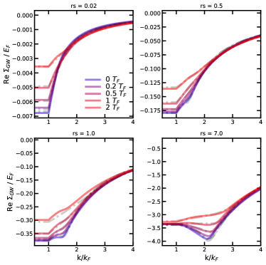
Figure 7: Our parametrization (solid) to the real part of $\Sigma_{GW}(T)$ (gray, dash-dotted) for $r_{s}$ = 0.02, 0.5, 1.0 and 7.0 (blue to red).

Appendix B Model for $\textnormal{Im}\ \Sigma_{GW}$

The imaginary part of the finite temperature GW self-energy, $\textnormal{Im}\ \Sigma_{GW}(T)$, is parametrized by

$$\frac{\textnormal{Im}\ \Sigma_{GW}(X)}{E_{F}} = \begin{cases}\eta_{1}(r_{s})kt+\eta_{2}(r_{s})kt^{\frac{3}{2}}\\ +\eta_{3}(r_{s})k^{2}t+\eta_{4}(r_{s})k^{2}t^{\frac{3}{2}}\\ +\eta_{5}(r_{s})k^{\frac{3}{2}}t+\eta_{6}(r_{s})k^{\frac{3}{2}}t^{\frac{3}{2}}\\ +\eta_{7}(r_{s})k+\eta_{8}(r_{s})k^{2}\\ +\eta_{9}(r_{s})k^{\frac{3}{2}}\\ +\frac{\textnormal{Im}\ \Sigma_{GW}(r_{s},x=1,t)}{E_{F}},x<\lambda(r_{s},t)\\ \\ \sigma\sum_{i=1}^{6}\tilde{\eta}_{i}(r_{s})\beta_{i}(t)k^{-i},x\geq\lambda(r_{s},t)\end{cases}$$ (14)

where $\eta_{i}(r_{s}),\tilde{\eta}(r_{s})=\eta_{i1}r_{s}+\eta_{i2}r_{s}^{3/2}+\eta_{i3}r_{s}^{2}$ and $\sigma$ is the standard deviation of the data points used. The function $\lambda(r_{s},t)$ is given by

$$\lambda(r_{s},t) = \bigg{(}1+\tanh\bigg{[}\frac{r_{s}-\frac{1}{2}}{p_{1}}\bigg{]}\bigg{)}$$ (15)

$$\times\bigg{(}p_{2}r_{s}+\eta_{1}(t)\bigg{)}+\eta_{2}(t)$$

and Im $\Sigma$ at the Fermi level, $k_{F}$, is parametrized by:

$$\frac{\textnormal{Im}\ \Sigma_{GW}(r_{s},x=1,t)}{E_{F}} = \nu_{1}(t)r_{s}^{\frac{1}{2}}+\nu_{2}(t)r_{s}$$ (16)

$$+\nu_{3}(t)r_{s}^{\frac{3}{2}}+\beta_{4}(t)r_{s}^{\frac{5}{2}}$$

where $\nu_{i}(t)=\nu_{i1}t+\nu_{i2}t^{3/2}+\nu_{i3}t^{2}$. The fittings of Eq. (14), Eq. (15) and Eq. (16) are done for two temperature regions: $t<0.5$ and $t\geq 0.5$, and two density regions: $r_{s}<0.2$ and $r_{s}\geq 0.2$.

The final model is a linear combination of the left and right regions in Eq. (14). The left region is weighted by the Fermi function $w=1/\{1+\exp[15\big{(}k-1.1\lambda(r_{s},t)\big{)}]\}$ and the right side by $1-w$. In addition, to prevent spurious negative values at very low $t$, we clip any negative values to be zero. The resulting parametrization is shown in Fig. 8. The absolute mean error for our parametrization is $\approx$ 0.006 $E_{F}$.

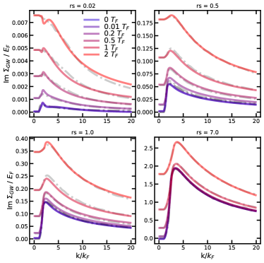
Figure 8: Our parametrization (solid) to the imaginary part of $\Sigma_{GW}(T)$ (gray, dash-dotted) for $r_{s}$ = 0.02, 0.5, 1.0 and 7.0 (blue to red).

References

- Peyrusse [2008] O. Peyrusse, Journal of Physics: Condensed Matter 20, 195211 (2008).
- Recoules and Mazevet [2009] V. Recoules and S. Mazevet, Phys. Rev. B 80, 064110 (2009).
- Cho et al. [2011] B. I. Cho, K. Engelhorn, A. A. Correa, T. Ogitsu, C. P. Weber, H. J. Lee, J. Feng, P. A. Ni, Y. Ping, A. J. Nelson, D. Prendergast, R. W. Lee, R. W. Falcone, and P. A. Heimann, Phys. Rev. Lett. 106, 167601 (2011).
- Dorchies et al. [2015] F. Dorchies, V. Recoules, J. Bouchet, C. Fourment, P. M. Leguay, B. I. Cho, K. Engelhorn, M. Nakatsutsumi, C. Ozkan, T. Tschentscher, M. Harmand, S. Toleikis, M. Störmer, E. Galtier, H. J. Lee, B. Nagler, P. A. Heimann, and J. Gaudin, Phys. Rev. B 92, 144201 (2015).
- Engelhorn et al. [2015] K. Engelhorn, V. Recoules, B. I. Cho, B. Barbrel, S. Mazevet, D. M. Krol, R. W. Falcone, and P. A. Heimann, Phys. Rev. B 91, 214305 (2015).
- Ogitsu et al. [2018] T. Ogitsu, A. Fernandez-Pañella, S. Hamel, A. A. Correa, D. Prendergast, C. D. Pemmaraju, and Y. Ping, Phys. Rev. B 97, 214203 (2018).
- Bolis et al. [2019] R. Bolis, J.-A. Hernandez, V. Recoules, M. Guarguaglini, F. Dorchies, N. Jourdain, A. Ravasio, T. Vinci, E. Brambrink, N. Ozaki, J. Bouchet, F. Remus, R. Musella, S. Mazevet, N. J. Hartley, F. Guyot, and A. Benuzzi-Mounaix, Physics of Plasmas 26, 112703 (2019).
- Jourdain et al. [2020] N. Jourdain, V. Recoules, L. Lecherbourg, P. Renaudin, and F. Dorchies, Phys. Rev. B 101, 125127 (2020).
- Li et al. [2021] Z. Li, W.-J. L. Li, C. Wang, D. Li, W. Kang, X.-T. He, and P. Zhang, Chinese Physics B 30, 057102 (2021).
- Faleev et al. [2006] S. V. Faleev, M. van Schilfgaarde, T. Kotani, F. Léonard, and M. P. Desjarlais, Phys. Rev. B 74, 033101 (2006).
- Hollebon et al. [2019] P. Hollebon, O. Ciricosta, M. P. Desjarlais, C. Cacho, C. Spindloe, E. Springate, I. C. E. Turcu, J. S. Wark, and S. M. Vinko, Phys. Rev. E 100, 043207 (2019).
- Cho et al. [2016] B. I. Cho, T. Ogitsu, K. Engelhorn, A. A. Correa, Y. Ping, J. W. Lee, L. J. Bae, D. Prendergast, R. W. Falcone, and P. A. Heimann, Scientific Reports 6, 18843 (2016).
- Denoeud et al. [2014] A. Denoeud, A. Benuzzi-Mounaix, A. Ravasio, F. Dorchies, P. M. Leguay, J. Gaudin, F. Guyot, E. Brambrink, M. Koenig, S. Le Pape, and S. Mazevet, Phys. Rev. Lett. 113, 116404 (2014).
- Karasiev et al. [2016] V. V. Karasiev, L. Calderín, and S. B. Trickey, Phys. Rev. E 93, 063207 (2016).
- Karasiev et al. [2018] V. V. Karasiev, J. W. Dufty, and S. Trickey, Phys. Rev. Lett. 120, 076401 (2018).
- Ichimaru et al. [1987] S. Ichimaru, H. Iyetomi, and S. Tanaka, Physics Reports 149, 91 (1987).
- Tanaka [2017] S. Tanaka, Contributions to Plasma Physics 57, 126 (2017).
- Tanaka [2016] S. Tanaka, The Journal of Chemical Physics 145, 214104 (2016).
- Perrot and Dharma-wardana [2000] F. Perrot and M. W. C. Dharma-wardana, Phys. Rev. B 62, 16536 (2000).
- Karasiev et al. [2014] V. V. Karasiev, T. Sjostrom, J. Dufty, and S. B. Trickey, Phys. Rev. Lett. 112, 076403 (2014).
- Groth et al. [2017] S. Groth, T. Dornheim, T. Sjostrom, F. D. Malone, W. M. C. Foulkes, and M. Bonitz, Phys. Rev. Lett. 119, 135001 (2017).
- Bunău and Calandra [2013a] O. Bunău and M. Calandra, Phys. Rev. B 87, 205105 (2013a).
- Seah and Dench [1979] M. P. Seah and W. A. Dench, Surface and Interface Analysis 1, 2 (1979).
- Cushing et al. [2018] S. K. Cushing, M. Zürch, P. M. Kraus, L. M. Carneiro, A. Lee, H.-T. Chang, C. J. Kaplan, and S. R. Leone, Structural Dynamics 5, 054302 (2018).
- Rehr and Albers [2000] J. J. Rehr and R. C. Albers, Rev. Mod. Phys. 72, 621 (2000).
- Korringa [1947] J. Korringa, Physica 13, 392 (1947).
- Kohn and Rostoker [1954] W. Kohn and N. Rostoker, Phys. Rev. 94, 1111 (1954).
- Dupree [1961] T. H. Dupree, Annals of Physics 15, 63 (1961).
- Beeby and Edwards [1967] J. L. Beeby and S. F. Edwards, Proceedings of the Royal Society of London. Series A. Mathematical and Physical Sciences 302, 113 (1967).
- Morgan [1966] G. J. Morgan, Proceedings of the Physical Society 89, 365 (1966).
- Casida [1995] M. Casida, Phys. Rev. A 51, 2005 (1995).
- Benedict et al. [2002] L. X. Benedict, C. D. Spataru, and S. G. Louie, Phys. Rev. B 66, 085116 (2002).
- Kas and Rehr [2017] J. J. Kas and J. J. Rehr, Phys. Rev. Lett. 119, 176403 (2017).
- Allen and Mitrović [1983] P. B. Allen and B. Mitrović (Academic Press, 1983) pp. 1–92.
- Hedin [1965] L. Hedin, Phys. Rev. 139, A796 (1965).
- Tan et al. [2021] T. S. Tan, J. J. Kas, and J. J. Rehr, Phys. Rev. B 104, 035144 (2021).
- Martin et al. [2016] R. M. Martin, L. Reining, and D. M. Ceperley, Interacting Electrons: Theory and Computational Approaches (Cambridge University Press, 2016).
- Bunău and Calandra [2013b] O. Bunău and M. Calandra, Phys. Rev. B 87, 205105 (2013b).
- Taillefumier et al. [2002] M. Taillefumier, D. Cabaret, A.-M. Flank, and F. Mauri, Phys. Rev. B 66, 195107 (2002).
- Gougoussis et al. [2009] C. Gougoussis, M. Calandra, A. P. Seitsonen, and F. Mauri, Phys. Rev. B 80, 075102 (2009).
- Sham and Kohn [1966] L. J. Sham and W. Kohn, Phys. Rev. 145, 561 (1966).
- Mustre de Leon et al. [1991] J. Mustre de Leon, J. J. Rehr, S. I. Zabinsky, and R. C. Albers, Phys. Rev. B 44, 4146 (1991).
- Ankudinov et al. [1998] A. L. Ankudinov, B. Ravel, J. J. Rehr, and S. D. Conradson, Phys. Rev. B 58, 7565 (1998).
- Mahan [2000] G. Mahan, Many-Particle Physics (Springer, 2000).
- Arista and Brandt [1984] N. R. Arista and W. Brandt, Phys. Rev. A 29, 1471 (1984).
- Kas et al. [2021] J. J. Kas, F. D. Vila, C. D. Pemmaraju, T. S. Tan, and J. J. Rehr, Journal of Synchrotron Radiation 28, 1801 (2021).
- Rehr et al. [2010] J. J. Rehr, J. J. Kas, F. D. Vila, M. P. Prange, and K. Jorissen, Phys. Chem. Chem. Phys. 12, 5503 (2010).
- Karasiev et al. [2019] V. V. Karasiev, S. B. Trickey, and J. W. Dufty, Phys. Rev. B 99, 195134 (2019).
- [49] The FLEUR code (version max-6.0): www.flapw.de.
- Weinert et al. [1982] M. Weinert, E. Wimmer, and A. J. Freeman, Phys. Rev. B 26, 4571 (1982).
- Alekseeva et al. [2018] U. Alekseeva, G. Michalicek, D. Wortmann, and S. Blügel, in Euro-Par 2018: Parallel Processing, edited by M. Aldinucci, L. Padovani, and M. Torquati (Springer International Publishing, Cham, 2018) pp. 735–748.
- Perdew and Zunger [1981] J. P. Perdew and A. Zunger, Phys. Rev. B 23, 5048 (1981).
- Rehr et al. [1994] J. J. Rehr, C. H. Booth, F. Bridges, and S. I. Zabinsky, Phys. Rev. B 49, 12347 (1994).
- Kittel [2005] C. Kittel, Introduction to solid state physics, 8th ed. (Wiley, Hoboken, NJ, 2005) p. 20.
- Kiyono et al. [1978] S. Kiyono, S. Chiba, Y. Hayasi, S. Kato, and S. Mochimaru, Japanese Journal of Applied Physics 17, 212 (1978).
- Kas et al. [2007] J. J. Kas, A. P. Sorini, M. P. Prange, L. W. Cambell, J. A. Soininen, and J. J. Rehr, Phys. Rev. B 76, 195116 (2007).
- Kas et al. [2009] J. J. Kas, J. Vinson, N. Trcera, D. Cabaret, E. L. Shirley, and J. J. Rehr, Journal of physics. Conference series 190, 10.1088/1742 (2009).
- Lundqvist [1967] B. I. Lundqvist, Physik der kondensierten Materie 6, 206 (1967).
- Hedin and Lundqvist [1971] L. Hedin and B. I. Lundqvist, Journal of Physics C: Solid State Physics 4, 2064 (1971).