The core population and kinematics of a massive clump at early stages: an ALMA view

Abstract

High-mass star formation theories make distinct predictions on the properties of the prestellar seeds of high-mass stars. Observations of the early stages of high-mass star formation can provide crucial constraints, but they are challenging and scarce. We investigate the properties of the prestellar core population embedded in the high-mass clump AGAL014.492-00.139, and we study the kinematics at the clump and the clump-to-core scales. We have analysed an extensive dataset acquired with the ALMA interferometer. Applying a dendrogram analysis to the Band 7 $\rm\text{o-}H_{2}D^{+}$ data, we identified 22 cores. We have fitted their average spectra in local-thermodinamic-equilibrium conditions, and we analysed their continuum emission at $0.8\,\rm mm$. The cores have transonic to mildly supersonic turbulence levels and appear mostly low-mass, with $M_{\mathrm{core}}<30\,\rm M_{\odot}$. Furthermore, we have analysed Band 3 observations of the $\rm N_{2}H^{+}$ (1-0) transition, which traces the large scale gas kinematics. Using a friend-of-friend algorithm, we identify four main velocity coherent structures, all of which are associated with prestellar and protostellar cores. One of them presents a filament-like structure, and our observations could be consistent with mass accretion towards one of the protostars. In this case, we estimate a mass accretion rate of $\dot{M}_{\mathrm{acc}}\approx 2\times 10^{-4}\rm\,M_{\odot}\,yr^{-1}$. Our results support a clump-fed accretion scenario in the targeted source. The cores in prestellar stage are essentially low-mass, and they appear subvirial and gravitationally bound, unless further support is available for instance due to magnetic fields.

1 Introduction

High-mass stars dominate the energetic of the interstellar medium (ISM), mainly due to feedback during their whole life cycle. Despite their importance, however, their formation process is significantly less known that the low-mass counterpart. From the theoretical point of view, two main families of models have been developed. The core-accretion (or core-fed) model is a scaled-up version with respect to the low-mass process (McKee & Tan, 2003). It predicts the existence of high mass prestellar cores (HMPCs, $M_{\mathrm{core}}=$ several tens of solar masses), which are virialised either due to turbulence or to the contribution of magnetic pressure, that collapse as a whole (Tan et al., 2013, 2014). In the clump-fed or competitive accretion scenarios, instead, early fragmentation in high-mass clumps leads to the formation of essentially low-mass cores, which keep accreting mass from the dense surrounding environment also during the initial protostellar stages (Bonnell et al., 2001; Bonnell & Bate, 2006; Smith et al., 2009). In order to distinguish among the existing theories, observational constraints on the properties of the initial stages of high-mass star formation are needed, in particular in terms of core masses and properties of accretion.

These observations are however challenging, since high-mass stars are intrinsically rarer and on average more distant than low-mass ones. The birthplace of high-mass stars is to be found in the heavily obscured environments of infrared dark clouds (IRDCs, Rathborne et al. 2006). In particular, IRDCs that are dark at $24$ and $70\,\rm\mu m$ are supposed to host the earliest evolutionary stages of high-mass star formation (Tan et al., 2013; Sanhueza et al., 2013; Guzmán et al., 2015). Several studies have hence targeted IRDCs with interferometric facilities, such as the Atacama Large Millimeter/submillimeter Array (ALMA, as done by Zhang et al. 2015; Ohashi et al. 2016; Contreras et al. 2018; Svoboda et al. 2019; Sanhueza et al. 2019; Morii et al. 2021), or the Submillimeter Array (SMA, see for instance Sanhueza et al., 2017; Li et al., 2019; Pillai et al., 2019). Multiple works unveiled that the lack of emission at mid-infrared wavelengths as seen with single-dish facilities (e.g. the Spitzer Space Telescope) does not guarantee a complete lack of star formation activity, due to the high extinction that characterises high-mass star-forming regions (see e.g. Tan et al., 2016; Pillai et al., 2019; Li et al., 2020; Morii et al., 2021; Tafoya et al., 2021).

In this context, the ALMA Survey of $70\,\mu$m dark High-mass clumps in Early Stages survey (ASHES; Sanhueza et al., 2019) targeted twelve IRDCs with ALMA Band 6 observations. In the first paper of the series, the authors studied the clumps fragmentation using the continuum emission at $1.3\,$mm, identifying $\approx 300$ cores, none of which appears more massive than $30\,\rm M_{\odot}$. Continuum emission together with spectral line observations have the potential to provide a more complete picture of star-forming regions, in particular in terms of evolutionary stage assessment. For instance, outflow tracers (e.g. CO, SiO), or so-called warm transitions, which have high upper level energies ($E_{\mathrm{u}}>20-30\,\rm K$), can be used to identify signs of protostellar activity, such as outflow emission or gas heating (see e,g, Sanhueza et al., 2012; Li et al., 2020).

In the hunt for HMPCs, it is crucial to find a good and unambiguous tracer of the prestellar phases. Deuterated species appear promising to this aim. At low temperatures ($T<20\,\rm K$) and high densities ($n\gtrsim 10^{5}\,\rm cm^{-3})$ found in prestellar gas, most C- and O-bearing species are frozen out onto dust grains (Caselli et al., 1999; Bacmann et al., 2002). This contributes to increasing the abundance of $\rm H_{2}D^{+}$, the precursor of deuterated species in the gas phase, since this molecule is predominantly destroyed by reaction with CO (e.g. Ceccarelli et al., 2014, and references therein). This results in a boost of deuteration, and deuterated molecules can therefore be good probes of cold and dense gas.

Redaelli et al. (2021) reported the first $\rm\text{o-}H_{2}D^{+}$ observations with ALMA in high-mass star-forming regions and showed that this molecule is a good probe of prestellar conditions. The $\rm\text{o-}H_{2}D^{+}(1_{1,0}-1_{1,1})$ line was detected towards two intermediate-mass clumps (AG351 and AG354), at a spatial resolution of $\approx 1500\,$AU. The authors identified 16 cores in total, and estimated their masses from the continuum emission at $0.8\rm\,mm$. At $T_{\mathrm{dust}}=10\,$K, all cores are less massive than $10\,\rm M_{\odot}$, and the majority is subvirial, assuming negligible contribution to the stability from magnetic fields.

Molecular lines yield information also on the gas kinematics, which is of great importance when trying to investigate the accretion processes in high-mass clumps. Among the different tracers used, two important ones are ammonia (see e.g. Lu et al. 2018; Williams et al. 2018; Sokolov et al. 2019) and $\rm N_{2}H^{+}$ (Henshaw et al., 2014; Chen et al., 2019). The kinematics of high-mass star-forming regions can be studied by means of algorithms dedicated to identify the hierarchy in their filamentary structures, as done for instance by Peretto et al. (2014); Chen et al. (2019); Henshaw et al. (2019); Wang et al. (2020). Many of these works report the detection of velocity gradients usually interpreted as gas motions, linked to accretion flows towards cores or hubs (see for instance Hacar et al., 2022, and references therein).

The $70\,\mu\rm m$-dark clump AGAL014.492-00.139 (hereafter AG14) has an estimated mass of $5200\,\rm M_{\odot}$ and it is located at a distance of $3.9\,\rm kpc$ (Sanhueza et al., 2019). It belongs to the ATLASGAL TOP100 sample (Giannetti et al., 2014; König et al., 2017), a statistically significant sample of high-mass clumps at different evolutionary stages in the inner Galaxy. AG14 was also included among the targets of the ASHES project: Sanhueza et al. (2019) identified 37 cores in continuum, 25 of which are associated with warm line or outflow emission. This point was investigated further by Li et al. (2020), who used $\rm CO$ and $\rm SiO$ observations with ALMA, and found that six cores are associated with outflows. In particular, four present bipolar emission. Throughout this work, we will refer to these cores as protostellar (or protostars). More recently, Sakai et al. (2022) studied the emission of several deuterated molecules ($\rm N_{2}D^{+}$, $\rm DCO^{+}$, and DCN) found in ALMA Band 6.

In this work, we present an extensive ALMA dataset on AG14, from $90$ up to $370\rm\,GHz$ in Sect. 2, consisting of Band 3 data covering the $\rm N_{2}H^{+}$ (1-0) line, Band 7 data of the $\rm\text{o-}H_{2}D^{+}(1_{1,0}-1_{1,1})$ line, and Band 6 data of the $\rm N_{2}D^{+}$ (3-2) transition (already published in Sakai et al. 2022). These different lines are used to trace distinct parts of the clump. $\rm H_{2}D^{+}$ is mainly destroyed by reactions with CO, and it is hence sensitive to temperature rising beyond the CO desorption temperature ($\approx 20\,\rm K$). Furthermore, its $\rm\text{o-}H_{2}D^{+}(1_{1,0}-1_{1,1})$ transition has a critical density of $n_{\mathrm{c}}\approx 10^{5}\,\rm cm^{-3}$ (Hugo et al., 2009), hence this line is an ideal tracer of cold and dense gas at the core scales. $\rm N_{2}H^{+}$ is also a well known high-density tracer. Its first rotational transition has a critical density of $6\times 10^{4}\rm\,cm^{-3}$, and it presents an isolated hyperfine component well separated from the others also in cases of large linewidths ($\sigma_{\mathrm{V}}\lesssim 2-4\,$$\rm km\,s^{-1}$). This component is usually optically thin or only moderately optically thick (Sanhueza et al., 2012; Barnes et al., 2018; Fontani et al., 2021). In the intracloud gas in high-mass clumps, the $\rm N_{2}H^{+}$ transition is excited over large scales. For all these reasons, $\rm N_{2}H^{+}$ represents an ideal probe of the clump and clump-to-core kinematics. Finally, $\rm N_{2}D^{+}$ is also a high-density tracer, but Giannetti et al. (2019) studied the correlation between the $\rm\text{o-}H_{2}D^{+}(1_{1,0}-1_{1,1})$ and the $\rm N_{2}D^{+}$ (3-2) transitions in three clumps embedded in the G351.77-0.51 complex, using single-dish data from APEX. The main result of those authors was an anticorrelation between the abundances of the two molecular species. This was explained as an evolutionary effect: in the prestellar phase, as time evolves, the abundance of $\rm\text{o-}H_{2}D^{+}$ is expected to lower, mainly due the conversion to its doubly and triply deuterated forms (see also Sabatini et al. 2020). $\rm N_{2}D^{+}$ instead forms later, and then its abundance keep increasing, since it can be formed also from $\rm D_{2}H^{+}$ and $\rm D_{3}^{+}$ (see for instance the chemical model of Sipilä et al., 2013, 2015). These findings hinted to the possibility of using the abundance ratio between $\rm N_{2}D^{+}$ and $\rm\text{o-}H_{2}D^{+}$ as an evolutionary indicator, and we aim to investigate this point in AG14 with the available data.

The paper is organised as follows. The observations are presented in Sect. 2. In the analysis, we first investigate the core population embedded in the clump, using the $\rm\text{o-}H_{2}D^{+}(1_{1,0}-1_{1,1})$ data (Sect. 3.1). We then present the clump-to-core kinematic properties in Sect. 3.2, based on the analysis of $\rm N_{2}H^{+}$ (1-0) data. In Sect. 3.3 we analyse the correlation between the $\rm\text{o-}H_{2}D^{+}$ and the $\rm N_{2}D^{+}$ emission in the identified cores, and Sect. 4 contains a discussion and the concluding remarks of this work.

2 Observations

The observations used in this work are described in the following subsections, and the main technical details (e.g. angular resolution, sensitivity,…) are summarised in Table 1. If the data have already been published, we refer to the corresponding publication.

Table 1: Observational parameters

Observation	Beam size	Spatial res.	$rms$	Spectral res.
Band 7
Continuum $0.5\,\rm mm$	$0^{\prime\prime}.66\times 0^{\prime\prime}.50$, $PA=-73.4$°	$2600\rm AU\times 2000AU$	$0.8\,\rm mJy/beam$	-
$\rm\text{o-}H_{2}D^{+}(1_{1,0}-1_{1,1})$	$0^{\prime\prime}.67\times 0^{\prime\prime}.50$, $PA=-73.4$°	$2600\rm AU\times 2000AU$	$100\,\rm mK$	$0.20\,$$\rm km\,s^{-1}$
Band 6
Continuum $1.34\,\rm mm$	$1^{\prime\prime}.29\times 0^{\prime\prime}.85$, $PA=72.5$°	$5000\rm AU\times 3300AU$	$0.17\,\rm mJy/beam$	-
$\rm N_{2}D^{+}$ (3-2)	$1^{\prime\prime}.44\times 1^{\prime\prime}.00$, $PA=74.8$°	$5600\rm AU\times 3900AU$	$180\,\rm mK$	$0.17\,$$\rm km\,s^{-1}$
Band 3
$\rm N_{2}H^{+}$ (1-0)	$2^{\prime\prime}.86\times 1^{\prime\prime}.61$, $PA=74.7$°	$11200\rm AU\times 6200AU$	$110\,\rm mK$	$0.20\,$$\rm km\,s^{-1}$

2.1 Band 7 observations

The Band 7 data were observed during Cycle 6 as part of the ALMA project 2018.1.00331.S (PI: Bovino) in three runs (November 2018 and March-April 2019). The observations, performed as a single-pointing, made use of both the Main Array (12m-array, 45 antennas) and the 7m-array (12 antennas), with baselines ranging from $7$ to $645\,\rm m$. The quasars J1924-2914, J1911-2006, J1733-1304, and J1751+0939 were used as calibrators. The spectral setup comprises four spectral windows (SPWs). The first one, dedicated to the observation of the $\rm\text{o-}H_{2}D^{+}(1_{1,0}-1_{1,1})$ transition, is centred at the frequency $\nu_{\mathrm{rest}}=372421.3558\,\rm MHz$ (Jusko et al., 2017), and has a resolution of $244\,\rm kHz$ (corresponding to $0.20\,$$\rm km\,s^{-1}$ at $372\,\rm GHz$) and a total bandwidth of $500\,\rm MHz$. The second SPW is dedicated to continuum, with a total bandwidth of $1.85\,\rm GHz$ around the frequency of $371\,\rm GHz$.

At these frequencies, and with the used configuration, the maximum recoverable scale is $\theta_{\mathrm{MRS}}\approx 20^{\prime\prime}$, the primary beams of the main array and of ACA are $17^{\prime\prime}$ and $30^{\prime\prime}$, respectively, and the angular resolution is $\approx 0^{\prime\prime}.6$ (corresponding to $\approx 2300\,\rm AU$ at the distance of $3.9\,\rm kpc$). The total observing time was $6.0\,\rm h$ (7m-array) and $2.5\,\rm h$ (12m-array). During the observations, the precipitable water vapour was typically $0.4\,\mathrm{mm}<PWV<0.6\,\mathrm{mm}$. The average system temperature values are found in the range $300-400\,\rm K$ for the SPW containing the $\rm\text{o-}H_{2}D^{+}(1_{1,0}-1_{1,1})$ line. The data were calibrated by the standard pipeline (casa, version 5.4; McMullin et al. 2007). From a first inspection of the dirty maps, the emission both in continuum and in line appear very extended in the whole Field-of-View (FoV). We therefore applied a modified weight of $2.4$ to the ACA observations, similarly to what was done in Redaelli et al. (2021). After a few tests, this choice appeared the ideal compromise to maximise the recovery of the large-scale flux, without downgrading too much the final angular resolution.

We imaged the data using the tclean task of the software casa (version 5.6), in interactive mode. We used the natural weighting and the multiscale deconvolver algorithm (Cornwell, 2008) (scales: $0,5,15$). In order to avoid oversampling, both the continuum and the line images have been re-gridded in order to ensure 3 pixels per beam minor axis, in agreement with the Nyquist theorem. Table 1 summarises the achieved sensitivities and resolutions. The molecular line data have been converted into the brightness temperature $T_{\mathrm{b}}$ scale, using the gain G computed as:

$$G=1.222\times 10^{6}\frac{1}{\nu^{2}\theta_{\mathrm{min}}\theta_{\mathrm{maj}}}=26\,\rm mK/(mJy\,beam^{-1})\;,$$ (1)

where $\nu$ is the frequency in GHz and $\theta_{\mathrm{min/maj}}$ are the beam sizes along the minor and major axes, respectively, expressed in arcsec.

Figure 1 shows the integrated intensity map of the $\rm\text{o-}H_{2}D^{+}$ line, computed in the velocity range $36-43\,$$\rm km\,s^{-1}$, masking channels with a signal lower than $1\sigma$. The contours show the distribution of the continuum emission at $0.8\,\rm mm$. Similarly to what has been noticed in Redaelli et al. (2021) in two different sources, the morphology of the continuum and of the line emission are in general different. Several bright peaks identified in dust thermal emission lack a counterpart in $\rm\text{o-}H_{2}D^{+}$ emission above the $3\sigma$ level.

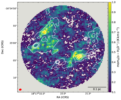
Figure 1: The colorscale shows the integrated intensity of the $\rm\text{o-}H_{2}D^{+}(1_{1,0}-1_{1,1})$ line, where pixels below the $3\sigma$ level have been masked. The mean uncertainty on the map is $1\sigma=60\,\rm mK\,$$\rm km\,s^{-1}$. The contours show the continuum emission at levels from $2$ to $11\sigma$, in steps of $3\sigma$. Both continuum and line data are shown prior to primary beam correction. The beam size and scalebar are indicated in the bottom left and right corners, respectively.

2.2 Band 6 observations

The Band 6 data of the continuum emission and of the $\rm N_{2}D^{+}$ (3-2) line at $\nu_{\mathrm{rest}}=231321.8283\,\rm MHz$ have been published by Sanhueza et al. (2019) and Sakai et al. (2022), respectively, and we refer to those papers for a complete description of the observations and of the data reduction. Briefly, the data were observed in Cycle 3 (Project ID: 2015.1.01539.S; PI: Sanhueza), with the 12, array, the 7m array (baselines ranging from 8 to 330 m), and the Total Power (the latter for spectral lines only). The data were acquired as mosaics, consisting of 10 pointings for the 12m array and 3 for the 7m array.

The spectral window containing the $\rm N_{2}D^{+}$ line was imaged using the automatic clean script yclean (Contreras et al., 2018), which uses natural weighting and multiscale deconvolver (scales: 0, 3, 10, 30). The casa version 5.4 was used for the imaging. To allow a better comparison with the $\rm\text{o-}H_{2}D^{+}(1_{1,0}-1_{1,1})$ data (see Sect. 3.3), we have excluded the Total Power data for this analysis, and the maximum recoverable scale is $\theta_{\mathrm{MRS}}=35^{\prime\prime}$. The final angular resolution of the 12m+7m combined datacube is $\approx 1^{\prime\prime}.0\times 1.^{\prime\prime}4$, and the pectral resolution is $0.17\,$$\rm km\,s^{-1}$. The data have been converted from the flux scale to temperature scale through the gain $G=15\,\rm mK/(mJy\,beam^{-1})$, computed with Eq. 1.

2.3 Band 3 observations

The Band 3 data were collected as part of project 2018.1.00299.S (PI: Contreras), during Cycle 6. The data consist of 12m array observations (performed in December 2018 and April 2019), 7m array observations (performed in January 2019), and Total Power (April 2019), with baseline ranging from $9.0\,\rm m$ to $500\rm\,m$. The average precipitable water vapour was in the range $4.6\,\mathrm{mm}<PWV<6\rm\,mm$. The quasars J2000-1748, J1517-2422, and J1832-2039 were used as calibrators for the 12m-array data, whilst J1751+0939, J2056-4714, and J1911-2006 were used during the 7m-array observations.

In this paper, we focus on the $\rm N_{2}H^{+}$ (1-0) transition at $93.174\,\rm GHz$, which was targeted by a dedicated SPW with a spectral resolution of $61\,\rm kHz$, corresponding to a velocity resolution of $0.20\,$$\rm km\,s^{-1}$ at the $\rm N_{2}H^{+}$ frequency. The primary beam size at the $\rm N_{2}H^{+}$ frequency is $\approx 60^{\prime\prime}$ for the 12m array, and $\approx 110^{\prime\prime}$ for the 7m array. The line was imaged with Briggs weighting (robust = 0.5) and multiscale deconvolver, using the tclean task of the software casa (version 5.7). The scales used were $0,5,15,25$ times the pixel size ($0^{\prime\prime}.4$, corresponding to 1/4 of the beam minor axis, in agreement with the Nyquist sampling). The final beam size of the composite datacube (12m+7m+TP arrays), after primary-beam correction, is $2^{\prime\prime}.9\times 1.6^{\prime\prime}$. The fluxes where converted in temperature scale using Eq. 1, obtaining the gain $G=30\,\rm mK/(mJy\,beam^{-1})$. The maximum recoverable scale considering the 12m and 7m array configuration is $\theta_{\mathrm{MRS}}=85^{\prime\prime}$, but the Total Power observations further increase it.

3 Analysis

3.1 The prestellar core population

The $\rm\text{o-}H_{2}D^{+}(1_{1,0}-1_{1,1})$ emission traces cold and dense gas. In this Section, we describe the analysis of the Band 7 data aimed to identify the population of prestellar cores in the clump, and to study their properties.

3.1.1 Prestellar cores identification

Our aim is to use the $\rm\text{o-}H_{2}D^{+}(1_{1,0}-1_{1,1})$ data to identify structures (cores) which are in a early, prestellar stage. Similarly to what has been done in Redaelli et al. (2021), we use scimes (Colombo et al., 2015), which is based on the dendrogram algorithm (Rosolowsky et al., 2008) and analyses data in three-dimensional, position-position-velocity (ppv) space.

The first key step of scimes is the dilmasking masking technique, which maximises the information recoverable in low signal-to-noise ratio (S/N) data (see Rosolowsky & Leroy 2006). The code identifies regions where the $\rm S/N$ is higher than a given threshold ($\rm S/N_{lim}$), that however contain emission peaks brighter than a second threshold ($\rm S/N_{peak}$). After a few test, we set $\rm S/N_{peak}=2$, and $\rm S/N_{lim}=1.5$, consistent with our choice in Redaelli et al. (2021), which maximises the signal recovery. Another key parameter to build the dendrogram is the minimum height (in flux/brightness) that a structure must have to be catalogued as an independent leaf ($\Delta_{min}$). We set the minimum height of an identified structure on $\Delta_{min}=2.8\times rms$, where $rms=100\,\rm mK$ (this is the value obtained on the datacube before primary-beam correction, since scimes requires data with constant noise). We set the minimum number of channels that a leaf must span to $N\rm^{min}_{chan}=2$, and we mask structures smaller than three times the beam area. With these input parameters, we find 22 prestellar cores, shown in Fig. 2. Some of them appear to overlap in projection on the plane of the sky. This is due to the fact that scimes works in ppv space, and it is therefore able to identify distinct velocity components as belonging to different structures. We report in Table 2 the positions and sizes, expressed in terms of effective radius, of the whole sample of cores.

Figure 2 confirms the fact that continuum and $\rm\text{o-}H_{2}D^{+}$ emission do not perfectly correlate, as seen also in Fig. 1. The positions of the protostellar candidates found by Li et al. (2020), also shown in Fig. 2, are usually associated with peaks of continuum (with the exception of the one in the north-west corner), and either not associated with, or found at the edges of, the $\rm H_{2}D^{+}$-identified cores. In Appendix A we present a more detailed study of the continuum cores.

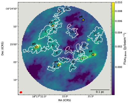
Figure 2: The cores identified in $\rm\text{o-}H_{2}D^{+}$ by scimes are shown as white contours, on top of the continuum emission. They are labelled in order of decreasing right-ascension. The star symbols show the position of the protostellar cores identified by Li et al. (2020), labelled in bold face. The beam size and scalebar are indicated in the bottom left and right corners, respectively.

Table 2: Core properties and best-fit results obtained fitting their average spectra with mcweeds. The $rms$ values are standard deviation over line-free channels. Uncertainties on $V_{\mathrm{lsr}}$, $\sigma_{\mathrm{V}}$, $N_{\mathrm{col}}$, one-dimension turbulent Mach number, and virial mass are expressed as 95% high probability density intervals (HPD).

Core id	Position		$R_{\mathrm{eff}}$	$rms$	$V_{\mathrm{lsr}}$	$\sigma_{\mathrm{V}}$	$N_{\mathrm{col}}$	$\mathcal{M}$	$M_{\mathrm{vir}}$
	RA(h:m:s.ss)	Dec (d:m:s.ss)	$10^{3}$AU	K	$\rm km\,s^{-1}$	$\rm km\,s^{-1}$	$\log_{10}(\rm cm^{-2})$		M⊙
1	$18:17:22.59$	$-16:25:1.35$	5.5	0.09	$38.26^{+0.06}_{-0.06}$	$0.38^{+0.07}_{-0.06}$	$13.20^{+0.06}_{-0.06}$	$1.84^{+0.42}_{-0.38}$	$4.8^{+1.7}_{-1.4}$
2	$18:17:22.41$	$-16:25:01.36$	2.4	0.07	$38.96^{+0.10}_{-0.11}$	$0.34^{+0.02}_{-0.02}$	$12.91^{+0.07}_{-0.07}$	$1.61^{+0.02}_{-0.02}$	$1.74^{+0.04}_{-0.04}$
3	$18:17:22.38$	$-16:24:56.44$	6.1	0.07	$40.33^{+0.04}_{-0.05}$	$0.40^{+0.02}_{-0.04}$	$13.27^{+0.04}_{-0.04}$	$2.01^{+0.11}_{-0.24}$	$6.1^{+0.6}_{-1.1}$
4	$18:17:22.29$	$-16:24:58.68$	2.5	0.07	$38.38^{+0.05}_{-0.05}$	$0.29^{+0.05}_{-0.05}$	$13.02^{+0.06}_{-0.06}$	$1.32^{+0.34}_{-0.32}$	$1.4^{+0.5}_{-0.4}$
5	$18:17:22.24$	$-16:25:0.27$	5.5	0.03	$38.43^{+0.04}_{-0.04}$	$0.40^{+0.04}_{-0.03}$	$13.04^{+0.03}_{-0.03}$	$2.00^{+0.22}_{-0.19}$	$5.5^{+1.0}_{-0.9}$
6	$18:17:22.22$	$-16:24:55.66$	5.1	0.04	$39.71^{+0.05}_{-0.05}$	$0.30^{+0.01}_{-0.01}$	$12.96^{+0.04}_{-0.04}$	$1.37^{+0.01}_{-0.01}$	$2.96^{+0.03}_{-0.03}$
7	$18:17:22.21$	$-16:24:53.65$	4.5	0.06	$40.42^{+0.04}_{-0.04}$	$0.36^{+0.04}_{-0.03}$	$13.16^{+0.04}_{-0.04}$	$1.74^{+0.22}_{-0.19}$	$3.6^{+0.7}_{-0.5}$
8	$18:17:22.21$	$-16:25:6.23$	4.5	0.06	$41.01^{+0.12}_{-0.13}$	$0.42^{+0.09}_{-0.09}$	$12.72^{+0.11}_{-0.10}$	$2.08^{+0.50}_{-0.52}$	$4.8^{+2.1}_{-1.7}$
9	$18:17:22.16$	$-16:25:2.31$	3.9	0.04	$39.23^{+0.03}_{-0.03}$	$0.30^{+0.03}_{-0.03}$	$12.96^{+0.04}_{-0.04}$	$1.38^{+0.20}_{-0.20}$	$2.3^{+0.4}_{-0.4}$
10	$18:17:22.10$	$-16:24:50.74$	3.7	0.21	$40.43^{+0.11}_{-0.12}$	$0.33^{+0.10}_{-0.09}$	$13.26^{+0.11}_{-0.14}$	$1.58^{+0.59}_{-0.55}$	$2.6^{+1.5}_{-1.1}$
11	$18:17:22.02$	$-16:25:4.36$	3.9	0.04	$41.21^{+0.06}_{-0.06}$	$0.33^{+0.01}_{-0.02}$	$12.76^{+0.05}_{-0.06}$	$1.60^{+0.04}_{-0.04}$	$2.7^{+0.1}_{-0.1}$
12	$18:17:21.97$	$-16:24:49.84$	2.9	0.33	$40.57^{+0.15}_{-0.14}$	$0.28^{+0.02}_{-0.05}$	$13.34^{+0.16}_{-0.16}$	$1.26^{+0.12}_{-0.12}$	$1.5^{+0.2}_{-0.2}$
13	$18:17:21.94$	$-16:25:1.57$	3.1	0.04	$38.86^{+0.05}_{-0.05}$	$0.21^{+0.04}_{-0.04}$	$12.50^{+0.08}_{-0.08}$	$0.83^{+0.29}_{-0.30}$	$1.0^{+0.3}_{-0.3}$
14	$18:17:21.87$	$-16:25:6.43$	3.2	0.07	$41.46^{+0.06}_{-0.05}$	$0.34^{+0.05}_{-0.05}$	$13.11^{+0.06}_{-0.06}$	$1.64^{+0.29}_{-0.28}$	$2.4^{+0.7}_{-0.6}$
15	$18:17:21.86$	$-16:24:56.45$	5.3	0.04	$39.55^{+0.04}_{-0.04}$	$0.22^{+0.03}_{-0.03}$	$12.76^{+0.06}_{-0.06}$	$0.91^{+0.21}_{-0.23}$	$1.9^{+0.4}_{-0.4}$
16	$18:17:21.84$	$-16:25:4.75$	2.4	0.08	$41.44^{+0.04}_{-0.04}$	$0.29^{+0.04}_{-0.04}$	$13.15^{+0.05}_{-0.05}$	$1.28^{+0.09}_{-0.18}$	$1.2^{+0.1}_{-0.2}$
17	$18:17:21.75$	$-16:25:2.60$	6.2	0.03	$39.28^{+0.03}_{-0.03}$	$0.24^{+0.03}_{-0.03}$	$12.77^{+0.04}_{-0.05}$	$1.02^{+0.19}_{-0.21}$	$2.5^{+0.5}_{-0.5}$
18	$18:17:21.68$	$-16:25:1.99$	2.7	0.06	$37.93^{+0.06}_{-0.06}$	$0.19^{+0.08}_{-0.06}$	$12.61^{+0.11}_{-0.12}$	$0.66^{+0.56}_{-0.49}$	$0.8^{+0.6}_{-0.3}$
19	$18:17:21.67$	$-16:25:3.87$	4.2	0.05	$41.34^{+0.02}_{-0.02}$	$0.27^{+0.02}_{-0.02}$	$13.20^{+0.03}_{-0.03}$	$1.25^{+0.13}_{-0.13}$	$2.2^{+0.3}_{-0.3}$
20	$18:17:21.63$	$-16:25:0.29$	3.7	0.06	$39.28^{+0.07}_{-0.07}$	$0.31^{+0.06}_{-0.06}$	$12.82^{+0.07}_{-0.08}$	$1.49^{+0.36}_{-0.34}$	$2.3^{+0.8}_{-0.7}$
21	$18:17:21.40$	$-16:24:56.93$	6.2	0.11	$40.25^{+0.04}_{-0.04}$	$0.29^{+0.03}_{-0.03}$	$13.35^{+0.05}_{-0.05}$	$1.35^{+0.20}_{-0.20}$	$3.5^{+0.7}_{-0.7}$
22	$18:17:21.35$	$-16:24:58.56$	3.6	0.14	$40.36^{+0.06}_{-0.06}$	$0.30^{+0.04}_{-0.05}$	$13.29^{+0.07}_{-0.08}$	$1.42^{+0.26}_{-0.28}$	$2.2^{+0.6}_{-0.5}$

3.1.2 Core properties from $\rm\text{o-}H_{2}D^{+}$ fitting

We perform a spectral fit of the $\rm\text{o-}H_{2}D^{+}(1_{1,0}-1_{1,1})$ in each core, in order to derive maps of the centroid velocity ($V_{\mathrm{lsr}}$), linewidth ($FWHM$), and column density $N_{\mathrm{col}}(\text{$\rm\text{o-}H_{2}D^{+}$})$. We use the parallelised version of the mcweeds code (Giannetti et al., 2017), which is based on the Weeds package of GILDAS (Maret et al., 2011). Weeds is able to produce synthetic spectra in LTE approximation based on a set of input parameters ($FWHM$, $V_{\mathrm{lsr}}$, molecular column density, excitation temperature, and source size), assuming that the line profile is Gaussian. mcweeds, instead, provides the framework to optimise the search for the best-fit solution of the parameters. The code analyses the spectrum in each pixel with Bayesian statistical models implemented using PyMC (Patil et al., 2010). In particular, we use a Markov chain Monte Carlo (MCMC) algorithm to sample the parameter space, with uninformative flat priors over the models’ free parameters. Similarly as in Redaelli et al. (2021), for each position the code performs 100000 iterations, with a burn-in of 1000 steps. For the excitation temperature, we assume $\text{$T_{\mathrm{ex}}$}=10\,\rm K$ (see for instance Caselli et al. 2008; Friesen et al. 2014; Redaelli et al. 2021). The initial guesses for the free parameters are selected individually for each core. mcweeds uses the line $FWHM$ as a free parameter, but here we show the velocity dispersion instead ($\sigma_{\mathrm{V}}=FWHM/(2\sqrt{2\,\rm ln(2)}$). Figure 3 shows the best-fit maps of the free parameters, obtained composing together those of the single cores. We show the best-fit parameter maps for each core individually in Appendix B.

Figure 3: Composite maps obtained showing together the results of mcweeds fit on the $\rm\text{o-}H_{2}D^{+}$ spectra for all the cores. Panel a): molecular column density, with contours of the $0.8\,\rm mm$ continuum emission overlaid (levels from $2$ to $11\sigma$, in steps of $3\sigma$); Panel b): $V_{\mathrm{lsr}}$ map, with the $\rm\text{o-}H_{2}D^{+}$-identified cores shown in black contours, and numeric labels; Panel c): velocity dispersion $\sigma_{\mathrm{V}}$ map; Panel d): one-dimensional turbulent Mach number. Note that in case of core overlapping, the maps show the results of only one of them. For the complete sets of maps of each individual core we refer to Appendix. B. The beam size and scalebar are indicated in the bottom left and right corners, respectively, of panel d).

The centroid velocity shows little gradient within each core. Excluding core 6 (one of the largest in terms of physical size) and core 12, the dispersion of $V_{\mathrm{lsr}}$ around the average is less than $0.20\,$$\rm km\,s^{-1}$. However, a clear change in $V_{\mathrm{lsr}}$ of the order of $3-4\,$$\rm km\,s^{-1}$ is visible at the clump level, in particular with changing declination. We can identify three separate groups: i) the southernmost cores have typical velocities of $>41\,$$\rm km\,s^{-1}$; ii) the cores in the central part of the clump present lower velocities ($V_{\mathrm{lsr}}$ $<40\,$$\rm km\,s^{-1}$). Group 1 and 2 overlap in the west part of the clump (see e.g. core 19, 17, and 18); iii) in the northern part of AG14 the cores have typical velocities of $40-40.5\,$$\rm km\,s^{-1}$. The presence of these three sub-populations of cores, with distinct velocities, suggests that AG14 presents a complex kinematics, with several velocity components that spatially overlap (see also the average spectra in Fig. 5). This is further investigated in Sect. 3.2.

To investigate the core properties in terms of velocity dispersion and column density, we present the density distribution of these two parameters in Fig. 4 (green colorscale), and compare it with the results for AG351 and AG354 obtained in Redaelli et al. (2021). We highlight that AG351 and AG354 are at about half of the distance with respect to AG14. However, the Band 7 data (both continuum and lines) were acquired with a higher angular resolution for AG14 ($\approx 0^{\prime\prime}.55$, to be compared with $\approx 0^{\prime\prime}.9$ for AG351 and AG354). Hence, the linear resolution of the data is only $\approx 25$% worse, allowing a fair comparison. The average $\rm\text{o-}H_{2}D^{+}$ column density in AG14 is $\langle N_{\mathrm{col}}\rangle=10^{13}\,\rm cm^{-2}$, which is consistent with the value obtained by Sabatini et al. (2020) with observations from the Atacama Pathfinder EXperiment (APEX), at a resolution ($17^{\prime\prime}$) comparable to the FoV of the ALMA data. The average velocity dispersion is $\langle\sigma_{\mathrm{V}}\rangle=0.30\,$$\rm km\,s^{-1}$. AG14 presents on average higher column density values than AG351.

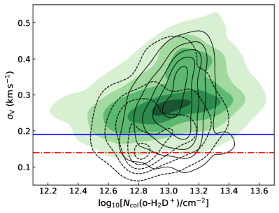
Figure 4: The green colorscale shows the normalised kernel density distribution of $\sigma_{\mathrm{V}}$ and $N_{\mathrm{col}}$ in AG14, with contour levels set on $[0.1,0.3,0.5,0.7,0.9]$. The same data are shown for AG351 with the dashed contours, and for AG354 with solid contours (taken from Redaelli et al. 2021; the $N_{\mathrm{col}}$ values have been corrected by a factor $\sqrt{\pi}$, see text for details). The horizontal blue solid and red dashed-dotted lines represent the sound speed and the thermal broadening of $\rm\text{o-}H_{2}D^{+}$, respectively, both at $10\,$K.

Furthermore, both clumps reported in Redaelli et al. (2021) showed very narrow lines, with a significant fraction on positions below both the isothermal sound speed at $10\,\rm K$ ($c_{\mathrm{s}}=0.19\,$$\rm km\,s^{-1}$, assuming a gas mean molecular weight $\mu=2.33$) and the thermal broadening of the $\rm\text{o-}H_{2}D^{+}(1_{1,0}-1_{1,1})$ at $10\,\rm K$ ($\sigma_{\mathrm{V,th}}=0.14\,$$\rm km\,s^{-1}$). On the contrary, in AG14 only 8% of the positions detected in $\rm\text{o-}H_{2}D^{+}$ present $\sigma_{V}<c_{\mathrm{s}}$ (to be compared with 36% and 23% in AG351 and AG354, respectively), and less than 1% are characterised by $\sigma_{\mathrm{V}}<\sigma_{\mathrm{V,th}}$ (17% and 7% in AG351 and AG354). The gas motions in AG14 hence appear less quiescent than in AG351 and AG354. We highlight that the derived velocity dispersion values might be overestimated, due to the limited spectral resolution of our observations. Lines narrower than $FWHM=0.6\,$$\rm km\,s^{-1}$ (corresponding to $\sigma_{\mathrm{V}}=0.25\,$$\rm km\,s^{-1}$), in fact, are resolved by less than three channels. However, the spectral resolution is the same for all three clumps, and therefore this problem would not affect the comparison between the sources. In Appendix C we discuss also the linewidth overestimation due to opacity effect, which is found to be at most 15% and only in the densest parts of the AG14.

From the total velocity dispersion $\sigma_{\mathrm{V}}$, the non-thermal contribution can be computed, in the assumption that the thermal and non-thermal contributions are independent and thus they sum in quadrature (see e.g. Myers et al., 1991):

$$\sigma_{\mathrm{V,NT}}=\sqrt{\sigma_{\mathrm{V}}^{2}-\sigma_{\mathrm{V,th}}^{2}}=\sqrt{\sigma_{\mathrm{V}}^{2}-\frac{k_{\mathrm{B}}T_{\mathrm{gas}}}{m_{\mathrm{H_{2}D^{+}}}}}\;,$$ (2)

where $m_{\mathrm{H_{2}D^{+}}}$ is the $\rm H_{2}D^{+}$ molecular mass (in g, 4 a.m.u.), $T_{\mathrm{gas}}$ is the gas temperature (assumed to be $10\,\rm K$), and $k_{\mathrm{B}}$ is the Boltzmann constant. The one-dimensional turbulent Mach number is then $\mathcal{M}=\sigma_{\mathrm{V,NT}}/c\rm_{s}$. The bottom-right panel of Fig. 3 shows the map of this parameter. In most of the cores, the turbulent motions are transonic or mildly supersonic ($\mathcal{M}=1-2$). A few cores, however, present subsonic non-thermal linewidhts (e.g. cores n. 15, 17, 18, and 19).

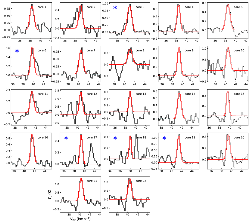
Figure 5: In black we show the average $\rm\text{o-}H_{2}D^{+}(1_{1,0}-1_{1,1})$ spectra obtained in each core (labelled at the top-right corner of each panel). The red histogram shows the best-fit obtained with mcweeds. The corresponding best-fit parameters are recorded in Table 2. Cores that overlap by at least 5% of their extension with another core are marked with a blue asterisk in the top-left corner of the panel.

3.1.3 Average core properties

An assessment of the dynamical state of each core can be obtained from the one-dimensional turbulent Mach number and the virial mass. These quantities are computed by fitting the averaged spectra within each core via mcweeds. The average spectra in each core, together with the obtained best-fit models, are shown in Fig. 5, and the best-fit values are presented in Table 2. In Fig. 5 we have highlighted with a blue asterisk those cores with significant overlap (at least 5% of their extension) with at least one other core. These cases present either multiple velocity components well separated in velocity (e.g. core 17 and 18), or broad wings and shoulders (core 6). We however select the initial guesses for the fit of the average spectra from the results of the pixel-by-pixel fit of each core, and mcweeds is hence able to identify and fit the correct velocity component.

From the $\sigma_{\mathrm{V}}$ values derived fitting the average spectra we computed the one-dimensional turbulent Mach number in each core, following the procedure described in Sect. 3.1.2. Furthermore, we have derived the total velocity dispersion of the gas ($\sigma_{\mathrm{dyn}}$) as:

$$\sigma_{\mathrm{dyn}}=\sqrt{\sigma_{\mathrm{NT}}^{2}+c_{\mathrm{s}}^{2}}\;,$$ (3)

from which we can derive the virial mass of the cores using the equation of Bertoldi & McKee (1992), in the assumption of uniform density (MacLaren et al., 1988):

$$M_{\mathrm{vir}}=\frac{5R_{\mathrm{core}}\sigma_{\mathrm{dyn}}^{2}}{G}=1200\times\left(\frac{R_{\mathrm{core}}}{\mathrm{pc}}\right)\left(\frac{\sigma_{\mathrm{dyn}}}{\mathrm{km\,s^{-1}}}\right)^{2}\rm{M_{\odot}}\;,$$ (4)

where for the $R_{\mathrm{core}}$ values we have used the effective radii listed in Table 2. This definition of the virial mass ignores contributes from magnetic fields and external pressure.

The values of $\mathcal{M}$ span the range $0.7-2.0$, with an average of $\langle\sigma_{\mathrm{V,NT}}/c\rm_{s}\rangle=1.4$. The turbulent motions in AG14 are transonic, or mildly supersonic. The $\sigma_{\mathrm{V,NT}}/c\rm_{s}$ values are significantly lower than the value reported by Sabatini et al. (2020) using APEX observations ($\sigma_{\mathrm{V,NT}}/c\rm_{s}=5.4$), most likely because the unresolved single-dish spectrum overestimates the linewidth, due to the velocity gradient that the ALMA data unveils ($\approx 4\,$$\rm km\,s^{-1}$) and the presence of several velocity components. The virial masses derived at $10\,\rm K$ are found within the range $0.8-6.1\,\rm M_{\odot}$, with 50% of the cores presenting $M\rm_{vir}<2.4\,M_{\odot}$. If the prestellar cores identified in $\rm\text{o-}H_{2}D^{+}$ are virialised, they are essentially low-mass.

In the analysis of the $\rm\text{o-}H_{2}D^{+}(1_{1,0}-1_{1,1})$ transition performed so far, we have assumed that the line opacity is low, and that the missing flux due to the filtering of the large scale emission from the interferometer is negligible. We discuss these points in further detail in Appendix  C.

3.1.4 Continuum emission

Further information on the core properties comes from the analysis of the continuum emission. In particular, we can estimate the core total mass ($M_{\mathrm{core}}$) using the equation:

$$M_{\mathrm{core}}=f\frac{D^{2}S_{\mathrm{tot}}}{B_{\nu}(T_{\mathrm{dust}})\kappa_{\nu}}\;,$$ (5)

where $f$ is the gas-to-dust ratio (assumed to be 100, Hildebrand 1983); $D$ is the source’s distance; $B_{\nu}(T_{\mathrm{dust}})$ is the Planck function at the frequency $\nu=371\,\rm GHz$ and temperature $T_{\mathrm{dust}}$; $S_{\mathrm{tot}}$ is the $0.8\,\rm mm$ total flux integrated within the contours of the $\rm\text{o-}H_{2}D^{+}$-identified cores, and $\kappa_{\nu}$ is the dust opacity at the frequency of the observations. For the latter, we use the power-law expression:

$$\kappa_{\nu}=\kappa_{0}\left(\frac{\nu}{\nu_{0}}\right)^{\beta}=1.71\,\rm cm^{2}\,g^{-1}\;,$$ (6)

in which we use $\beta=1.5$ for the dust emissivity index (Mezger et al., 1990; Walker et al., 1990) and $\kappa_{0}=10\,\rm cm^{2}\,g^{-1}$ for the dust opacity at the reference wavelength $\lambda_{0}=250\,\mu\rm m$ (Hildebrand, 1983; Beckwith et al., 1990). In the assumption of spherical symmetry and uniform gas distribution, we can evaluate the gas density as:

$${n\mathrm{(H_{2})}=\frac{3M_{\mathrm{core}}}{4\pi R_{\mathrm{eff}}^{3}\mu_{\mathrm{H_{2}}}m_{\mathrm{H}}}\;,}$$ (7)

where $m_{\mathrm{H}}$ and $\mu_{\mathrm{H_{2}}}=2.8$ are respectively the hydrogen mass and the gas mean molecular weight per hydrogen molecule (Kauffmann et al., 2008).

Table 3: Core properties derived from the continuum emission at $0.8\,\rm mm$. The core masses, volume densities, and virial parameters are computed at three distinct temperatures: 10, 15, and 20 K. The uncertainty on core masses and densities is 38%, whilst it is 43% on the virial parameter values.

Core id	$M_{\mathrm{core}}$	$n\rm(H_{2})$	$\alpha_{\mathrm{vir}}$	$M_{\mathrm{core}}$	$n\rm(H_{2})$	$\alpha_{\mathrm{vir}}$	$M_{\mathrm{core}}$	$n\rm(H_{2})$	$\alpha_{\mathrm{vir}}$
	$\mathrm{M_{\odot}}$	$10^{6}\rm cm^{-3}$		$\mathrm{M_{\odot}}$	$10^{6}\rm cm^{-3}$		$\mathrm{M_{\odot}}$	$10^{6}\rm cm^{-3}$
	$10\,\rm K$			$15\,\rm K$			$20\,\rm K$
1	$27\pm 10$	$4.9\pm 1.9$	$0.18\pm 0.08$	$13\pm 5$	$2.3\pm 0.9$	$0.40\pm 0.17$	$8\pm 3$	$1.4\pm 0.5$	$0.7\pm 0.3$
2	$1.9\pm 0.7$	$4.0\pm 1.5$	$0.9\pm 0.4$	$0.9\pm 0.3$	$1.8\pm 0.7$	$2.1\pm 0.9$	$0.5\pm 0.2$	$1.2\pm 0.4$	$3.6\pm 1.5$
3	$19\pm 7$	$2.5\pm 0.9$	$0.33\pm 0.14$	$9\pm 3$	$1.1\pm 0.4$	$0.8\pm 0.3$	$5\pm 2$	$0.7\pm 0.3$	$1.2\pm 0.5$
4	$2.2\pm 0.8$	$4.3\pm 1.6$	$0.6\pm 0.3$	$1.0\pm 0.4$	$2.0\pm 0.8$	$1.5\pm 0.6$	$0.6\pm 0.2$	$1.2\pm 0.5$	$2.5\pm 1.1$
5	$9\pm 3$	$1.5\pm 0.6$	$0.7\pm 0.3$	$3.9\pm 1.5$	$0.7\pm 0.3$	$1.5\pm 0.6$	$2.5\pm 0.9$	$0.4\pm 0.2$	$2.4\pm 1.0$
6	$10\pm 4$	$2.1\pm 0.8$	$0.31\pm 0.13$	$4.4\pm 1.7$	$1.0\pm 0.4$	$0.7\pm 0.3$	$2.8\pm 1.0$	$0.6\pm 0.2$	$1.2\pm 0.5$
7	$9\pm 4$	$3.1\pm 1.2$	$0.39\pm 0.17$	$4.3\pm 1.6$	$1.5\pm 0.6$	$0.9\pm 0.4$	$2.7\pm 1.0$	$0.9\pm 0.3$	$1.5\pm 0.6$
8	$6\pm 2$	$1.9\pm 0.7$	$0.8\pm 0.4$	$2.7\pm 1.0$	$0.9\pm 0.3$	$1.9\pm 0.8$	$1.7\pm 0.6$	$0.6\pm 0.2$	$3.1\pm 1.3$
10	$2.8\pm 1.1$	$1.6\pm 0.6$	$0.9\pm 0.4$	$1.3\pm 0.5$	$0.8\pm 0.3$	$2.2\pm 0.9$	$0.8\pm 0.3$	$0.5\pm 0.2$	$3.6\pm 1.6$
17	$8\pm 3$	$1.0\pm 0.4$	$0.32\pm 0.14$	$3.7\pm 1.4$	$0.5\pm 0.2$	$0.8\pm 0.3$	$2.3\pm 0.9$	$0.3\pm 0.1$	$1.3\pm 0.6$
18	$1.0\pm 0.4$	$1.6\pm 0.6$	$0.8\pm 0.3$	$0.5\pm 0.2$	$0.8\pm 0.3$	$1.9\pm 0.8$	$0.30\pm 0.11$	$0.5\pm 0.2$	$3.3\pm 1.4$
19	$13\pm 5$	$5\pm 2$	$0.16\pm 0.07$	$6\pm 2$	$2.5\pm 0.9$	$0.38\pm 0.16$	$3.9\pm 1.5$	$1.6\pm 0.6$	$0.6\pm 0.3$
21	$20\pm 7$	$2.4\pm 0.9$	$0.18\pm 0.08$	$9\pm 3$	$1.1\pm 0.4$	$0.42\pm 0.18$	$6\pm 2$	$0.7\pm 0.3$	$0.7\pm 0.3$
22	$8\pm 3$	$5.0\pm 1.9$	$0.28\pm 0.12$	$3.6\pm 1.4$	$2.3\pm 0.9$	$0.6\pm 0.3$	$2.3\pm 0.9$	$1.5\pm 0.6$	$1.1\pm 0.5$

Equation 5 and, as a consequence, Eq. 7 depend on the dust temperature. In the hypothesis that the line is excited in LTE conditions (which holds for $n(\mathrm{H_{2}})\gtrsim n_{\mathrm{cr}}\approx 10^{5}\,\rm cm^{-3}$, Hugo et al. 2009) and that the gas and dust are thermally coupled (which requires $n(\mathrm{H_{2}})\gtrsim 10^{4-5}\rm\,cm^{-3}$, Goldsmith 2001), we can assume that $T_{\mathrm{dust}}=T_{\mathrm{gas}}=T_{\mathrm{ex}}(\text{$\rm\text{o-}H_{2}D^{+}$})=10\,$K. However, in order to relax these assumptions and to take into consideration that locally the dust and gas temperatures could differ, we have computed the core masses and average densities at three temperatures, equal to 10, 15, and 20 K. The obtained values are summarised in Table 3. From this analysis, we exclude cores that are undetected in continuum, meaning that they lack of peak flux above the $3\sigma$ level. At $10\,\rm K$, the point-like mass sensitivity of our observations is $0.6\,\rm M_{\odot}$ ($3\sigma$ level). Due to the different morphology that the continuum and molecular line data present, as discussed in Sect. 3.1.1, eight cores are excluded.

Regarding uncertainties, we follow Sanhueza et al. (2017) (see in particular their Sect. 5.6), and we assume a 23% uncertainty on the dust-to-mass-ratio, and 28% uncertainty on the dust opacity. Furthermore, we assume a 10% uncertainty on the source’s distance. Hence, the uncertainty on the mass and on the density values are $38$%. In Equation 5, the total flux is computed integrating the continuum data within each core masks; in case of core overlap, naturally, this will cause an overestimation of their masses. This problem is more severe with increasing overlap area. We have estimated the significance of this bias using the method presented by Li et al. (2020) to decompose the dust-estimated masses of cores when spectroscopic data are available, in the hypothesis that the molecular transition is a high-density tracer (i.e. it traces densities higher than the threshold for dust-gas coupling) and is optically thin. Under these assumptions, which are both reasonably valid for our $\rm\text{o-}H_{2}D^{+}$ data, one can decompose the continuum flux into different cores according to the ratio of the line integrated intensity of each velocity component with respect to the total integrated intensity (computed over all the velocity components). We have performed this analysis for the five cores that overlap by more than 5% of their area (see also Fig. 5). We find that on average their masses are overestimated by 23%, i.e. less than the uncertainties here considered. We conclude that this possible bias does not affect significantly our results.

Focusing on the gas density values, we note that also assuming a higher dust temperature of 20 K, all the cores have average densities higher than $3\times 10^{5}\,\rm cm^{-3}$. This level is comparable to the critical density of the $\rm\text{o-}H_{2}D^{+}(1_{1,0}-1_{1,1})$ line, corroborating the assumption both of LTE conditions for this transition, and of dust-gas coupling. Regarding the masses, all cores are less massive than $30\,\rm M_{\odot}$ at any temperature value here considered. This is consistent with what is found by Sanhueza et al. (2019), who identified cores (at any evolutionary stage) in continuum Band 6 data. We however highlight that the lack of Total Power observations in continuum can lead to partial filter-out of the large scale emission, hence underestimating the mass values.

In Table 3 we report also the virial parameter values ($\alpha_{\mathrm{vir}}=M_{\mathrm{vir}}/M_{\mathrm{core}}$) at the three temperatures here considered. The uncertainty on $\alpha_{\mathrm{vir}}$ takes into account the 38% uncertainty on the core masses and a further 20% error, which corresponds to the average uncertainty on the virial mass values. At low dust temperature ($T_{\mathrm{dust}}=10\,\rm K$), all cores present $\alpha_{\mathrm{vir}}<1.0$, suggesting that they are both subvirial and gravitationally bound. Also at $T_{\mathrm{dust}}=15\,\rm K$, we derived $0.3\leq\alpha_{\mathrm{vir}}\leq 2.2$, and all cores are gravitationally bound ($\alpha_{\mathrm{vir}}<2$) within uncertainties. The virial parameter increaseas with temperature, but still at $T_{\mathrm{dust}}=20\,\rm K$ 50% of the cores in the sample are subvirial within uncertainties. In particular, the most massive cores present the lowest $\alpha_{\mathrm{vir}}$ values ($\alpha_{\mathrm{vir}}\lesssim 0.3$ for $\text{$M_{\mathrm{core}}$}\gtrsim 8\rm\,M_{\odot}$), in agreement with several observational results (see e.g. Kauffmann et al. 2013). This suggests that the largest cores in the sample are not in equilibrium, unless other sources of pressure (e.g. magnetic fields) contribute to the virialisation.

Singh et al. (2021) performed an extensive study regarding biases in the computation of the virial parameter that tend to lead to its underestimation. Those authors in particular discussed the role of i) neglecting the gas bulk motions in the calculation of $\sigma_{\mathrm{dyn}}$ and of ii) the subtraction of the background emission. They found that when these aspects are taken into account, many cores that appeared subvirial become instead virialised or supervirial. However, our analysis intrinsically limits this problem. Since $\sigma_{\mathrm{dyn}}$ is computed from averaged spectra in each core, bulk motions —if present— are already taken into account as they increase the velocity dispersion of the averaged signal. Furthermore, as noted also by Singh et al. (2021), interferometric observations naturally filter out the large scale emission, hence performing an approximate background subtraction. We conclude that these effects are likely negligible in our results.

We now discuss the properties of the most massive cores identified. Core 1, with $M_{\mathrm{core}}\approx 30\,M_{\odot}$ at $10\,\rm K$ is the most massive core and it is subvirial at any temperature value considered in this work. However, we have reasons to believe that this core is not in a prestellar stage. In fact, it overlaps with a continuum core associated with outflow emission and protostellar activity (see Appendix A). The continuum flux peak is found close to the edge of the core, suggesting that $\rm\text{o-}H_{2}D^{+}$ is tracing the part of the envelope which is still cold and dense enough to emit the $\rm\text{o-}H_{2}D^{+}(1_{1,0}-1_{1,1})$ transition. A similar discussion could be made for core 3, which has $M_{\mathrm{core}}=20\,\rm M_{\odot}$ (at 10 K) and it is subvirial, and it lays in close proximity to the protostar p5. Also core 21 has a similar mass, but unlike the other two, no protostellar core appears to be found in its surroundings. However, a significant continuum peak is found just outside its south-east edge. This peak is associated with the continuum-identified structure c8 (see Appendix A, where we speculated about the evolutionary stage of this core).

In Fig. 6 we compare the masses and sizes of the identified cores in AG351, AG354, and AG14 (at $T_{\mathrm{dust}}=10\,\rm{K}$). Cores in AG14 appear on average larger and more massive than in the other two clumps, as expected by the availability of a larger mass reservoir, since AG14 is a factor of $\approx 30$ more massive than the other two sources. In the figure, we also report several estimations of the threshold for high-mass star formation in the mass-size space. Krumholz & McKee (2008) derived analytically the surface density limit of $\Sigma\approx 1\,\rm g\,cm^{-2}$, which roughly translates into $M/\rm M_{\odot}=15\times 10^{3}(R/pc)^{2}$. From observational data of several IRDCs, Kauffmann & Pillai (2010) derived the relation $M/\rm M_{\odot}=870\,(R/pc)^{1.33}$, whilst more recently Baldeschi et al. (2017) reported $M/\rm M_{\odot}=1282\,(R/pc)^{1.42}$, based on the analysis of clouds in the Herschel Gould Belt survey. The most massive cores in AG14 sit well above all the relations here studied, and have therefore the potential to form high-mass stars in the future. However, since their masses are $M_{\mathrm{core}}\approx 10-30\,\rm{M_{\odot}}$, they still need to accrete significant mass from the surrounding environment, unless the star formation efficiency is locally high.

As previously noted, the angular resolutions of the observations of the three clumps are well matched to their distinct distances. However, the angular maximum recoverable scale is approximately the same for all the sources, which means that more large-scale flux is recovered in AG351 and AG354 with respect to AG14. This might affect the comparison between the core masses, which could be overestimated in AG351 and AG354 with respect to AG14. This however would not affect our conclusion that cores in the last clump are more massive than in the first two sources.

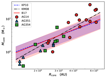
Figure 6: Core masses vs sizes in AG351 (blue triangles), AG354 (green squares), and AG14 (red circles). The thresholds for high-mass star formation described by Krumholz & McKee (2008), Kauffmann & Pillai (2010), and Baldeschi et al. (2017) are shown with the dash-dotted black curve, the dashed blue curve, and the solid red line, respectively. For the last two relations we also indicated uncertainties with shaded blue and red areas, which reflect differences in the dust opacity values used here and in those works. The uncertainties on $M_{\mathrm{core}}$ are $30$% (AG351 and AG354) and 38% (AG14).

3.2 The clump-to-core scale kinematics

The centroid velocity map obtained fitting the $\rm\text{o-}H_{2}D^{+}(1_{1,0}-1_{1,1})$ data, shown in Fig. 3, suggests a complex kinematics of the source, as indicated by the presence of several velocity components at many positions. In order to investigate the kinematics of AG14 at the clump scale, we have used ALMA Band 3 observations of the $\rm N_{2}H^{+}$ (1-0) transition. As illustrated in Sect. 1, this transition is better suited to trace the gas at larger scales than the $\rm\text{o-}H_{2}D^{+}(1_{1,0}-1_{1,1})$ data. Furthermore, the Band 3 data have a spatial resolution of $11200\rm AU\times 6180AU$ ($0.05\,\rm pc\times 0.03\,pc$), and they were acquired including Total Power observations (which are not available in the Band 7 dataset), which increases the sensitivity to the large scale emission. These observations are therefore ideal to probe the large-scale kinematics of the gas in which the cores identified in $\rm\text{o-}H_{2}D^{+}$ are embedded.

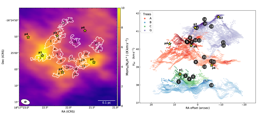
Figure 7: Left panel: the colorscale shows the integrated intensity of the isolated $\rm N_{2}H^{+}$ hyperfine component $F_{1}=0-1$. The white contours show the cores identified in $\rm\text{o-}H_{2}D^{+}$ (labelled with numbers), and the star symbols the positions of the protostars (labelled in bold face). The scalebar is indicated in the bottom-right corner. The white ellipse shows the beam size of the $\rm N_{2}H^{+}$ data, whilst the smaller grey ellipse represents the $\rm\text{o-}H_{2}D^{+}$ beam size. Right panel: position-velocity plot from the results of acorns. The plot is the projection in RA-velocity space of the 3D plot shown in Fig. 9. Right-ascension values are given as offsets with respect to the centre of the FoV (position $\rm RA=18^{h}17^{m}22^{s}.05$, $\rm Dec=-16\text{\degree}25^{\prime}01^{\prime\prime}.7$). The four main trees identified by acorns are shown with distinct colours, and the colorscale is determined by the peak intensity of the line, stretching linearly between $0\,K$ and 90% of the maximum $T_{\mathrm{peak}}$ in each tree. The positions of the prestellar and the protostellar cores are shown with the black circles and the yellow stars, respectively. Labels correspond to those in the left panel.

We focused on the isolated hyperfine component $F_{1}=0-1$ of the $\rm N_{2}H^{+}$ (1-0) transition, which is supposed to be optically thin or only moderately optically thick even at the high column densities found in high-mass star-forming regions (see for instance Sanhueza et al. 2012; Barnes et al. 2018; Fontani et al. 2021). The integrated intensity of this component is shown in the left panel of Fig. 7, where we overlap also the contours of the $\rm\text{o-}H_{2}D^{+}$ cores and the positions of the protostellar objects (star symbols). The field-of-view have been cut to the central $40^{\prime\prime}\times 40^{\prime\prime}$, focusing on the map area covered also by the Band 7 data. The $\rm N_{2}H^{+}$ emission is extended over almost the whole map coverage. The morphology appears filamentary, with several clumpy peaks of emission. Several of these peaks coincide with the position of protostellar candidates.

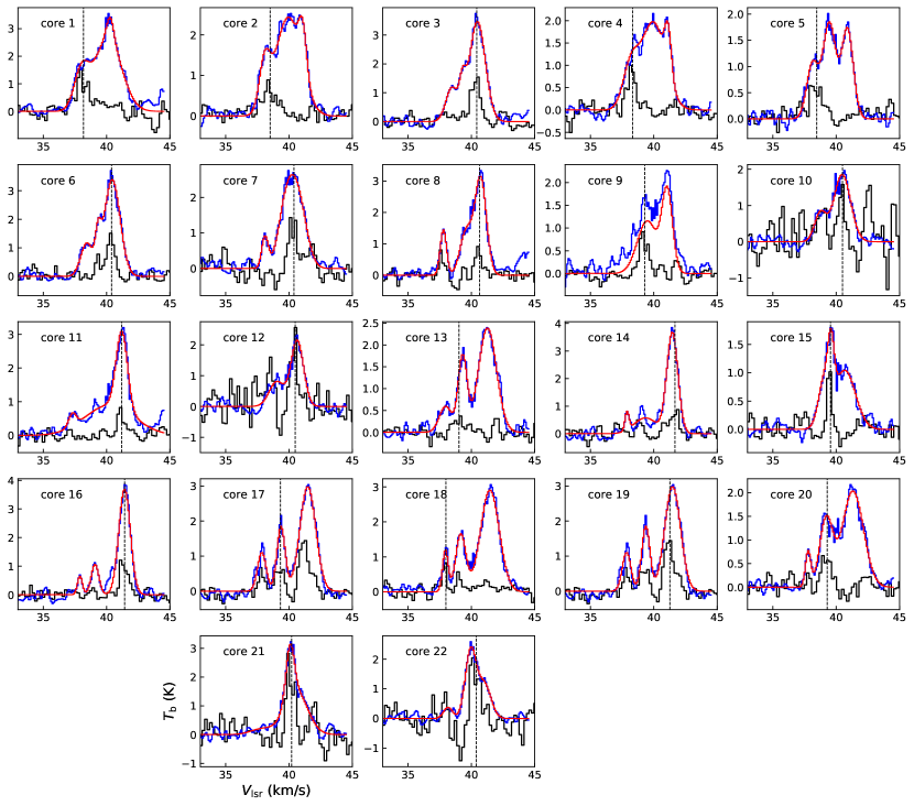
Figure 8: Comparison of the $\rm N_{2}H^{+}$ (1-0), in blue, and the $\rm\text{o-}H_{2}D^{+}(1_{1,0}-1_{1,1})$ spectra, in black, at the core positions. The spectra are taken at the position of the peak of $\rm\text{o-}H_{2}D^{+}$ integrated intensity. The red curves show the best model obtained fitting the $\rm N_{2}H^{+}$ data with three Gaussian components. The centroid velocity of the $\rm\text{o-}H_{2}D^{+}$ is shown with the vertical dashed line in each panel.

By a visual inspection of the datacube, it appears that three velocity components are present on a large extension of the source. We have hence proceeded with a three-components Gaussian fit using the pyspeckit package (Ginsburg & Mirocha, 2011). The technical details of the fitting routine are described in Appendix D. Figure 8 shows the comparison of the spectra of $\rm\text{o-}H_{2}D^{+}$ and $\rm N_{2}H^{+}$ at the peak of the $\rm\text{o-}H_{2}D^{+}$ integrated intensity, for each core identified in Sect. 3.1.1. The correspondence between the two species is remarkable. Every velocity components seen in $\rm\text{o-}H_{2}D^{+}$ is associated also with a $\rm N_{2}H^{+}$ component, whilst the opposite is not true. Furthermore, for corresponding components, $\rm\text{o-}H_{2}D^{+}(1_{1,0}-1_{1,1})$ tends to present narrower linewidths with respect to the $\rm N_{2}H^{+}$ line. These findings suggest the following scenario: over the whole clump, at least three gas components (separated in velocity usually by $0.5-1.0\,$$\rm km\,s^{-1}$) are visible, as traced by $\rm N_{2}H^{+}$, an abundant molecule that probes gas densities of $n\gtrsim 10^{4}\,\rm cm^{-3}$. Within these large scale structures, cores are formed, with significantly higher densities ($n>10^{5}\,\rm cm^{-3}$, see also Table 3). The gas within the cores is hence cold and dense, and it excites the $\rm\text{o-}H_{2}D^{+}(1_{1,0}-1_{1,1})$ emission. Arising from a more quiescent medium, the $\rm\text{o-}H_{2}D^{+}(1_{1,0}-1_{1,1})$ spectra are narrower than the $\rm N_{2}H^{+}$ ones, which instead are associated with larger scale, more turbulent gas, as suggested by the broader linewidths of this species.

The $\rm N_{2}H^{+}$ data allow us to study not only the kinematics within the cores (better traced by the $\rm\text{o-}H_{2}D^{+}$ data), but also that of the intraclump gas in which the cores are embedded, since we are able to link kinematically each core with one $\rm N_{2}H^{+}$ component. In order to investigate the gas structure in ppv space, we used the Agglomerative Clustering for ORganising Nested Structures (acorns; Henshaw et al. 2019). Similarly to scimes, acorns is a hierarchical clustering algorithm, which identifies structures and their hierarchical links in position-position-velocity space. However, unlike scimes, acorns is designed to work on already decomposed data. In other words, instead of working on the observed datacubes, it operates on the fitting results of the multi-component Gaussian fit previously described. The technical details about the acorns clustering are given in Appendix D. Using the terminology of Henshaw et al. (2019), acorns finds a forest of 18 trees in total, four of which contains $\approx 70$% of all data-points, and $\approx 80\%$ of the total flux. These trees present also the most complex hierarchical structures, containing each between two and seven leaves.

In Fig. 9 we show a screenshot of the 3D ppv plot of the four main trees found by acorns, together with the positions in ppv space of the prestellar and protostellar cores. For the prestellar ones, we use the positions of the peak intensity of the $\rm\text{o-}H_{2}D^{+}$ integrated intensity within each core, and the centroid velocity at the same position obtained with mcweeds (see Sect. 3.1.2). The properties of the protostellar cores are derived from Li et al. (2020), who used $\rm DCO^{+}$, $\rm N_{2}D^{+}$, or $\rm C^{18}O$ data to infer the systemic velocity values. A two-dimensional RA-velocity plot of the same data is shown in the right panel of Fig. 7.

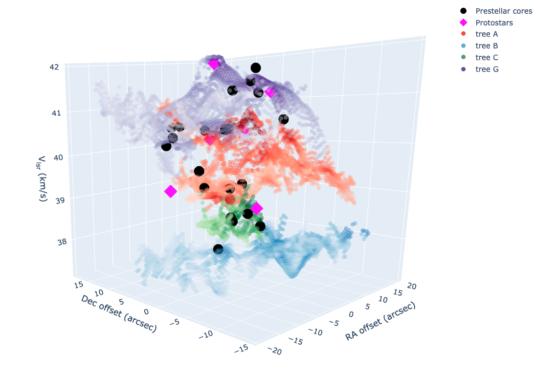
Figure 9: Screenshot of the ppv distribution of the four main trees identified by acorns, shown with distinct colors (A: red, B: blue, C: green, G: purple). The colorscale within each tree is determined by the peak intensity of the $\rm N_{2}H^{+}$ component. The black dots show the ppv position of the $\rm H_{2}D^{+}$ cores (taken at the peak of the line integrated intensity), whilst the magenta diamonds represent the positions of the protostellar cores, following Li et al. (2020). A permanent copy of this interactive plot is available at: http://theory-starformation-group.cl/sbovino/AG14_n2hp_light.html. The interactive version allows the reader to rotate the figure, to zoom in and out, and to see the numeric labels of the protostellar and prestellar cores by moving the cursor over.

All the four main trees identified by acorns appear associated with prestellar cores, and at least three of them host protostellar sources. These findings suggest that all of these structures have been or still are active in star formation. The structure at lower $V_{\mathrm{lsr}}$ values (shown in blue in Fig. 9, labelled B in Fig. 22) is the most coherent in velocity, as it span less than $1.0\,$$\rm km\,s^{-1}$, despite extending over $\approx 0.75\,\rm pc$ on the plane of the sky. It is also the most quiescent in star formation activity, based on the fact that it is associated with only one prestellar core, and no protostar. On the contrary, the tree coloured in green in Fig. 9 (cluster C in fig. 22), despite having a physical size of $\approx 0.15\,\rm pc$, contains four cores identified in $\rm\text{o-}H_{2}D^{+}$ and one protostellar core. The presence of tracers of both protostellar activity and of cold and dense gas suggest that the star formation is still on-going, and that the protostellar object is very young. The position of the protostellar core p1 is found in fact very close to the $\rm\text{o-}H_{2}D^{+}$ core 1, which hints to the fact that the protostellar envelope is still cold and dense enough to have a detectable abundance of $\rm\text{o-}H_{2}D^{+}$.

The remaining two trees (labels A and G in Fig. 22; shown respectively in red and purple in the right panel Fig. 7 and in Fig. 9) show a more complex and overlapping structure in ppv space, and they represent the most dynamically active part of the IRDC clump. At the same time they contain the large majority of cores identified in $\rm\text{o-}H_{2}D^{+}$ and three protostellar cores. This is indicative of the fact that this region of the clump is dynamically very active.

The two protostellar cores p4 and p6 are not associated in ppv space with any of the four main trees identified in $\rm N_{2}H^{+}$. After checking the whole cluster hierarchy found by acorns, however, p4 appears embedded in one of the minor trees identified (labelled as ’r’ in Fig. 22). The protostellar core p6, instead, has not correspondence in the forest identified by the algorithm. It still emits in the $\rm N_{2}H^{+}$ (1-0) transition (as can be seen in the integrated intensity map shown in Fig. 7), but with low flux, hence not fulfilling the S/N threshold that we require in the fitting algorithm. A possible interpretation of this observational evidence is that p6 has still an envelope, but this has been significantly cleared out by the protostellar activity, suggesting that this could be a more evolved protostar with respect to the others.

The tree labelled G (shown in purple in the right panel of Fig. 7 and in Fig. 9) is one of the largest identified trees, as alone it contains more than $20$% of the total data-points and $\approx 33$% of the total flux. It also presents a significant shift in velocity, extending from $\text{$V_{\mathrm{lsr}}$}=39.5\,$$\rm km\,s^{-1}$ to $42\,$$\rm km\,s^{-1}$. We now focus on its part connecting the two protostars p2 and p3 (see Fig.7), which presents the brightest peak intensities of the $\rm N_{2}H^{+}$ line. This section looks like a filament, elongating between the two protostellar cores, and containing four cores identified in the $\rm\text{o-}H_{2}D^{+}$ data (n. 11, 14, 16, and 19). The velocity is increasing from p3 towards p2.

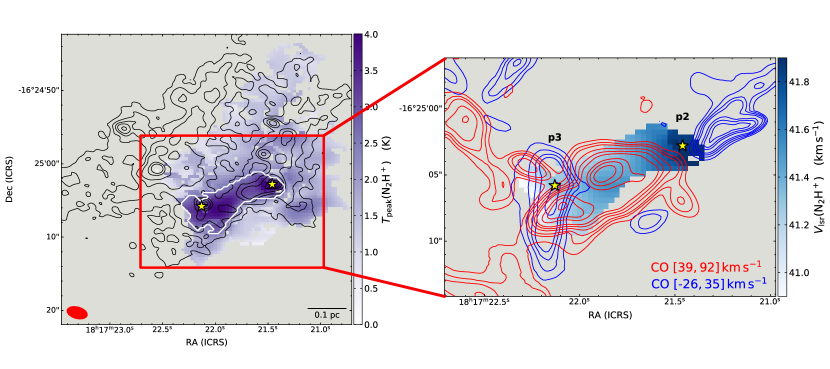
Figure 10: Left panel: The colorscale shows the peak intensity of the $\rm N_{2}H^{+}$ components associated with tree G, and the white contour shows the mask (corresponding to $T_{\mathrm{peak}}>2.5\,\rm K$) used to identify the filament studied in Sect. 3.2. The black contours show the continuum emission at 1.34 mm, at levels $[0.5,1.0,1.7,2.5,4.2,5.9]\,\rm mJy/beam$ (from Sanhueza et al. 2019). The red box indicates the position of the zoomed area shown in the right panel. Right panel: $V_{\mathrm{lsr}}$ map of tree G within the white contour of the left panel, with CO emission overlaid in contours (from Li et al., 2020). Contours are computed in the velocity indicated in the bottom-right corner, at levels: for the blue component, $[1.08,1.62,2.16,2.7,3.78,4.32,4.86]\,\rm Jy\,beam^{-1}\,$$\rm km\,s^{-1}$; for the red component, $[1.33,1.995,2.66,3.99,5.32,6.65,9.31,10.64,11.97]\,\rm Jy\,beam^{-1}\,$$\rm km\,s^{-1}$. The positions of protostars p2 and p3 are shown with yellow stars in both panels.

The left panel of Fig. 10 shows the map of peak intensity of points belonging to tree G. The material surrounding and linking the two protostar emits the brightest lines (with $T_{\mathrm{peak}}>2.5\,\rm K$) detected in the source. In the right panel of Fig. 10, we show the $V_{\mathrm{lsr}}$ map of this tree, with overlaid the contours of the outflows detected in the region by Li et al. (2020). The filamentary structure stretching between the two protostellar cores is found in correspondence with the red lobe of the outflow powered by protostar p2. However, the two features cannot coincide spatially, since their velocities are opposite: the outflow is red-shifted, and it has velocities higher than the local standard of rest velocity of protostar p2 ($V_{\mathrm{lsr}}=41.8\,$$\rm km\,s^{-1}$, according to Li et al. 2020), whilst the gas traced by the $\rm N_{2}H^{+}$ line is found at lower (blue-shifted) velocities than that of the protostar. Furthermore, the four $\rm H_{2}D^{+}$ cores embedded in the gas present low velocity dispersion ($\sigma_{\mathrm{V}}=0.27-0.34\,$$\rm km\,s^{-1}$) and transonic turbulent Mach number ($\mathcal{M}=1.2-1.6$, see Table 2), suggesting that the dense gas embedded in the filamentary structure is still cold and quiescent, and unperturbed by outflows.

We can thus speculate on the possible scenarios that would give raise to such an observed configuration. A first possibility is simply that we are seeing a bulk motion of the gas. The filament-like structures is moving, and the cores embedded into it participate to this motion. A second possibility is that the gas is flowing towards the protostellar core p2 (i.e. towards increasing velocities), and it accretes material onto the protostar, which in turn powers the bipolar outflow. In any case, the red outflow lobe of p2 and the filament-like structure are found on two distinct planes, which intersect at the position of the protostar, and they appear overlapping in RA-Dec space only due to projection effects.

Regardless of the real configuration, the observations unveil a gas flow along the filamentary structure, and it is possible to evaluate the mass-flow rate associated to it. If the correct scenario is the second we proposed, we can interpret this quantity as a mass accretion rate onto the protostar p2. To perform the calculation, we consider the filament as limited to those positions where $T_{\mathrm{peak}}>2.5\,\rm K$, since we want to focus on the denser portion of the gas traced by the $\rm N_{2}H^{+}$ (1-0) line. This region, shown with the white contour in the left panel of Fig. 10, has a width of $0.08-0.12\rm\,pc$, which are typical values for filaments (see e.g. Arzoumanian et al. 2011, 2019; Palmeirim et al. 2013; Sabatini et al. 2019), and a length of $\approx 0.26\rm\,pc$. It spans $1\,$$\rm km\,s^{-1}$ in velocity, from $40.9\,$$\rm km\,s^{-1}$ close to the protostar p3 to $41.9\,$$\rm km\,s^{-1}$ around p2. The velocity gradient is hence $\nabla V=3.85\,\rm km\,s^{-1}\,pc^{-1}$. To estimate the total mass of the filament ($M_{\mathrm{fil}}$), we employ again Eq. 5. We use the continuum emission detected in Band 6 at $1.34\,\rm mm$, since its FoV and resolution are closer to the Band 3 data with respect to the Band 7 ones. The flux density contained within the mask shown in Fig. 10 is $F_{\mathrm{fil}}=85\rm\,mJy$. A significant contribution to this flux level comes from the bright emission of the cores p2 and p3, which are $16$ and $15\rm\,mJy$, respectively (Sanhueza et al., 2019). In these cores, the emission likely arises from the warmer envelope surrounding the protostellar object, and we hence subtract it from $F_{\mathrm{fil}}$, since we are interested on the flow of gas not associated with the envelope of the protostars. The dust opacity at $1.34\,$mm, computed following Eq. 6, is $0.81\rm\,cm^{2}\,g^{-1}$. Assuming $T_{\mathrm{dust}}=10\,\rm K$, we obtain $M_{\mathrm{fil}}=57\,\rm M_{\odot}$. The mass accretion rate is then $\dot{M}_{\mathrm{acc}}=M_{\mathrm{fil}}\times\nabla V=2.2\times 10^{-4}\,\rm M_{\odot}\,yr^{-1}$. We stress again that this is the rate at which the mass flows along the filamentary structure. The scenario in which it actually corresponds to an accretion motion is only one of the possibilities that would explain the observations. In order to definitely assess if this is the case, more information, in particular on the protostars (i.e. their masses, luminosities, evolutionary stages,…) would be helpful.

In the following, we discuss the sources of uncertainties that affect the physical quantities just determined. First of all, there is the uncertainty on the mass, which accounts for $\approx 40$% (see Sect. 3.1.4), that comes from uncertainties in the dust-to-gas ratio, in the source’s distance, and in the dust opacity. Furthermore, the inclination $i$ of the filament with respect to the plane of the sky is unknown, and it affects the value of $\dot{M}_{\mathrm{acc}}$ by a factor $\tan{i}$ (see e.g. Chen et al. 2019). If the inclination varies in the range $30-60$°, the derived value of the accretion rate changes up to $70$%. Due to these considerations, with a conservative approach we assume that the derived $\dot{M}_{\mathrm{acc}}$ value is correct within a factor of two. Within the uncertainties, the value we found is in agreement with measurements in similar sources: for instance, Lu et al. (2018) found $\dot{M}_{\mathrm{acc}}=(1-2)\times 10^{-4}\,\rm M_{\odot}\,yr^{-1}$ in filaments belonging to four high-mass star-forming regions, whilst Chen et al. (2019) derived $\dot{M}_{\mathrm{acc}}=(0.2-1.3)\times 10^{-4}\,\rm M_{\odot}\,yr^{-1}$ in several filaments identified in the infrared dark cloud G14.225-0.506. Sanhueza et al. (2021) derived $\dot{M}_{\mathrm{acc}}=(0.9-2.5)\times 10^{-4}\,\rm M_{\odot}\,yr^{-1}$ in a hot core embedded in the high-mass star-forming region IRAS 18089-1732, even though at smaller spatial scales ($\approx 10000\,$AU). In Li et al. (2022), authors studied the accretion in a filament in the high-mass star-forming region NGC6334S, deriving $\dot{M}_{\mathrm{acc}}=0.3\times 10^{-4}\,\rm M_{\odot}\,yr^{-1}$. Furthermore, this value is also in agreement with the results of numerical simulations (see e.g. Wang et al., 2010; Kuiper et al., 2016).

The critical line mass of a filament, in the approximation of isothermal cylindrical shape, is (Ostriker, 1964):

$$m_{\mathrm{c}}=\frac{2c_{\mathrm{s}}^{2}}{G}=17\left(\frac{T_{\mathrm{K}}}{10\rm\,K}\right)\rm\,M_{\odot}\,pc^{-1}\;.$$ (8)

The line mass of the filamentary-like structure in AG14 is $m=M_{\mathrm{fil}}/L_{\mathrm{fil}}=220\rm\,M_{\odot}\,pc^{-1}$, i.e. significantly higher than its critical value, which suggests that this structure is out of hydrostatic equilibrium. One could naturally wonder whether this is consistent with the possible scenario of accretion flow that has been discussed. In particular, it is worth comparing the timescales for accretion ($t_{\mathrm{acc}}$) and free-fall collapse ($t_{\mathrm{ff}}$), at least in terms of orders of magnitude. The former can be approximated by the ratio between the mass reservoir and the accretion rate: $t_{\mathrm{acc}}=M_{\mathrm{fil}}/\dot{M}_{\mathrm{acc}}=2.6\times 10^{5}\,\rm yr$. To estimate the time necessary for a filament to fully collapse onto its axis, we use Eq. 18 of Hacar et al. (2022), which in turn was derived from Pon et al. (2012); Toalá et al. (2012):

$$t_{\mathrm{ff}}=1.9\left(\frac{L_{\mathrm{fil}}}{FWHM_{\mathrm{fil}}}\right)^{0.5}\left(\frac{n_{0}}{10^{3}\,\mathrm{cm^{-3}}}\right)^{-0.5}\,\rm Myr\;,$$ (9)

where $L_{\mathrm{fil}}/FWHM_{\mathrm{fil}}=2.6$ is the filament aspect ratio (i.e. the ratio between its length $L_{\mathrm{fil}}=0.26\,$pc and its width $FWHM_{\mathrm{fil}}=0.1\,$pc), and $n_{0}$ is the filament central density at the spine. Since we are interested only in a rough estimation of this quantity, we test the range of densities found in the cores, i.e. $n_{0}=10^{5}-10^{6}\,\rm cm^{-3}$, obtaining $t_{\mathrm{ff}}=1-3\times 10^{5}\,\rm yr$. We conclude that the two timescales are comparable, and hence the filament would have time to accrete a significant fraction of its mass onto p2 before collapsing.

3.3 Comparison between $\rm\text{o-}H_{2}D^{+}$ and $\rm N_{2}D^{+}$

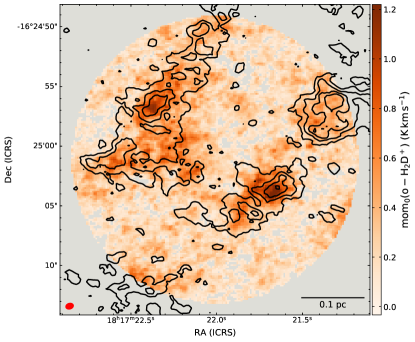
Figure 11: The colorscale shows the integrated intensity of the $\rm\text{o-}H_{2}D^{+}(1_{1,0}-1_{1,1})$ transition as in Fig. 1. The black contours shows the $\rm N_{2}D^{+}$ (3-2) integrated intensity (computed as for $\rm\text{o-}H_{2}D^{+}$, see Sect. 2). The levels are: $[7,11,15,19]\sigma$, where $1\sigma=100\rm\,mK\,km\,s^{-1}$.

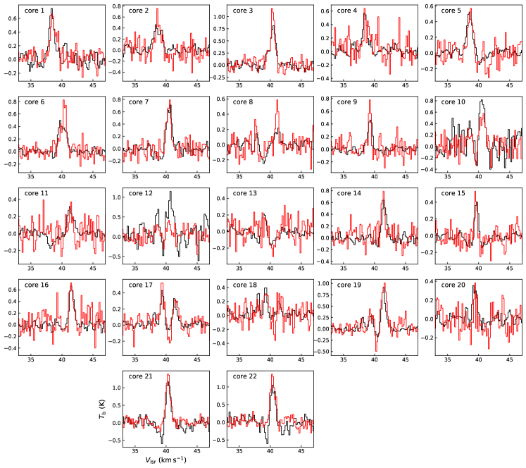
Figure 12: Comparison between the average $\rm N_{2}D^{+}$ (3-2) and $\rm\text{o-}H_{2}D^{+}(1_{1,0}-1_{1,1})$ lines in each core (labelled at the top-left corner of each panel). $\rm N_{2}D^{+}$ data are shown with the red histograms, whilst $\rm\text{o-}H_{2}D^{+}$ ones are shown with the black curves. Note that the $\rm\text{o-}H_{2}D^{+}$ data have been smoothed to the same beam size of the $\rm N_{2}D^{+}$ cube before extracting the average spectra, which thus are not identical to the ones presented in Fig. 5.

The cores identified in Sect. 3.1.1 using $\rm\text{o-}H_{2}D^{+}$ data are formed by cold and dense gas that should be in a prestellar stage, even though we have evidence that a minority of cores are found in close proximity to protostellar cores (in ppv space), such as core 1 (close to protostar p1), or cores 3, 6, and 7 (close to p5). We can speculate that in these cases the $\rm\text{o-}H_{2}D^{+}$ emission is tracing the part of the protostellar envelopes that is still cold enough that the desorption of CO from the dust grains has not happened yet. This is confirmed by depletion maps derived from $\rm C^{18}O$ (2-1) observations of AG14 at $1^{\prime\prime}.3$ of resolution, which show that the depletion factor is high ($f_{\mathrm{D}}>50$) even around protostellar cores (Sabatini et al., 2022). This suggests that ALMA observations at resolution of $\approx 1^{\prime\prime}$ are tracing the dense and still cold envelope around protostellar objects, where the feedback of the protostar has not affected the gas yet. However, even the remaining cores could still belong to distinct evolutionary stages. To these regards, we have mentioned that Giannetti et al. (2019) studied the correlation between the $\rm\text{o-}H_{2}D^{+}(1_{1,0}-1_{1,1})$ and the $\rm N_{2}D^{+}$ (3-2) transitions in three clumps embedded in the G351.77-0.51 complex, using single-dish data from APEX. The main result of those authors was an anticorrelation between the abundances of the two molecular species, possibly due to evolutionary effects. Their findings hinted to the possibility of using the abundance ratio between $\rm N_{2}D^{+}$ and $\rm\text{o-}H_{2}D^{+}$ as an evolutionary indicator.

In Fig. 11 we show the comparison between the integrated intensities of the $\rm N_{2}D^{+}$ (3-2) and the $\rm\text{o-}H_{2}D^{+}(1_{1,0}-1_{1,1})$ transitions. The two tracers appear quite correlated spatially, but some differences are visible. For instance, in the north-west part of the source, the $\rm N_{2}D^{+}$ line has a bright peak, which is not seen in $\rm\text{o-}H_{2}D^{+}$. Furthermore, the $\rm N_{2}D^{+}$ transition seems more extended, even though we must highlight a possible observational bias: despite we excluded the Total Power observations from the Band 6 dataset, its maximum recoverable scale is still almost twice that of the $\rm\text{o-}H_{2}D^{+}$ data, hence making the former more sensitive to large-scale emission.

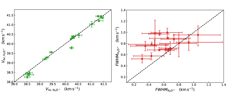
Figure 13: Left panel:Comparison of the centroid velocities obtained with mcweeds on the $\rm N_{2}D^{+}$ and $\rm\text{o-}H_{2}D^{+}$ average spectra in the cores where both species have been detected above the $3\sigma$ level. The black dashed line shows the $1:1$ relation. Right panel: Same as in the left panel, but for the linewidths.

In order to further explore the comparison at the core level, we compared the average spectra of $\rm\text{o-}H_{2}D^{+}(1_{1,0}-1_{1,1})$ and $\rm N_{2}D^{+}$ (3-2) in each core. Since the Band 6 data have a lower resolution of $1^{\prime\prime}.4\times 1^{\prime\prime}.0$, we first smoothed the Band 7 data to this beam size, to allow for a proper comparison. Both spectral cubes have been regridded to the same coordinate grid. The spectral resolution of the two datasets is comparable ($0.20\,$$\rm km\,s^{-1}$ for $\rm\text{o-}H_{2}D^{+}$ and $0.17\,$$\rm km\,s^{-1}$ for $\rm N_{2}D^{+}$). The comparison of the average spectra is shown in Fig. 12. The similarities between the line profiles of the two tracers are remarkable, both in terms of intensity and of line shapes. In four cores (12, 13, 18, and 20) the $\rm N_{2}D^{+}$ transition is not detected above the $3\sigma$ level, but we highlight that the $rms$ of the $\rm N_{2}D^{+}$ spectra is on average $\approx 2.5$ times worse than in the corresponding $\rm\text{o-}H_{2}D^{+}$ spectra.

We have fitted the average spectra shown in Fig.12 with mcweeds. We assumed $T_{\mathrm{ex}}=10\,\rm K$ also for $\rm N_{2}D^{+}$, for which we take into consideration the hyperfine splitting due to the ${}^{14}\rm N$ nuclei, according to the CDMS database. Figure 13 shows the comparison of the best-fit values for the centroid velocity and $FWHM$ for the two tracers in the cores where both are detected above $3\sigma$. The $V_{\mathrm{lsr}}$ values align very well, considering the uncertainties, with the 1:1 relation (shown with the black-dashed curve), highlighting that the two molecular emissions arise from similar spatial regions within the source. Concerning the linewidhts, the right panel of Fig. 13 shows that for 80% of the cores the $\rm\text{o-}H_{2}D^{+}$ transition presents broader lines with respect to $\rm N_{2}D^{+}$. This can be partially due to opacity effect, since the $\rm\text{o-}H_{2}D^{+}(1_{1,0}-1_{1,1})$ can be moderately optically thick, leading to a 15% overestimation of the linewidth (see Appendix C). The presence of the hyperfine splitting in the $\rm N_{2}D^{+}$ (3-2) transition, instead, reduces this problem. Furthermore, we highlight the difference in the critical density of these two tracers (one order of magnitude higher for the $\rm N_{2}D^{+}$ line than for the $\rm\text{o-}H_{2}D^{+}$ transition).

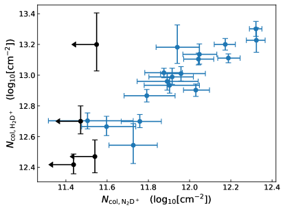
Figure 14: Same as Fig. 13, but for the column densities. For the four cores where $\rm N_{2}D^{+}$ is not detected, we show upper limits (in black).

In Fig. 14 we report the correlation between the column density values of $\rm\text{o-}H_{2}D^{+}$ and $\rm N_{2}D^{+}$. For the cores undetected in $\rm N_{2}D^{+}$, we report $3\sigma$-upper limits computed based on the $rms$ in each core and the average linewidths of the detected cores ($<FWHM>=0.62\,$$\rm km\,s^{-1}$). We found a discrepancy with the anti-correlation trend found by Giannetti et al. (2019), since the column density of $\rm N_{2}D^{+}$ and $\rm\text{o-}H_{2}D^{+}$ appear well correlated, for the cores detected in both tracers. However, we highlight a fundamental difference between our analysis and that of Giannetti et al. (2019). Those authors selected cores in continuum emission, and then analysed the molecular emission. Our analysis, instead, is intrinsically biased towards core with bright $\rm\text{o-}H_{2}D^{+}$ emission, since we used this species to identify core-like substructures. Furthermore, Giannetti et al. (2019) investigated the clump level scales, and therefore the anti-correlation reflected averaged clump properties. In this work, on the contrary, we resolve the core scales in a highly dynamically active environment, which further complicate a direct comparison between the two works.

It is worth commenting on the four cores undetected in $\rm N_{2}D^{+}$ emission. They present narrow $\rm\text{o-}H_{2}D^{+}$ lines ($\sigma_{\mathrm{V}}=0.18-0.27\,$$\rm km\,s^{-1}$, smaller than the average velocity dispersion of all cores in the clump), hinting to cold and quiescent gas. According to the analysis of the continuum emission (see Sect. 3.1.4 and Table 3), three of them are undetected in continuum emission, and the last one (18) is the least massive of the sample ($M_{\mathrm{core}}\lesssim 1.0\rm\,M_{\odot}$). The non-detection of $\rm N_{2}D^{+}$ can be then explained by two scenarios: i) these cores are not dense enough to excite the $\rm N_{2}D^{+}$ transition that has an higher critical density with respect to that of the $\rm\text{o-}H_{2}D^{+}(1_{1,0}-1_{1,1})$ line; ii) alternatively, the lack of continuum emission can be explained if the gas and dust temperatures are so low ($<10\,\rm K$) that the dust thermal emission at $0.8\rm\,mm$ is not bright; in this case, the cores would be in early evolutionary stage, and perhaps the $\rm N_{2}D^{+}$, a late-type species, has not yet formed in detectable quantities. In this case, the core masses estimated in Sect. 3.1.4 could be underestimated.

4 Discussion and Conclusions

In this work, we have investigated the dynamical and kinematic properties of AG14, from the core to the clump scales, analysing ALMA data at spatial resolution from $\sim$ 2000 to $\sim$ 12000 AU ($0.01-0.06\,\rm pc$). Using Band 7 $\rm\text{o-}H_{2}D^{+}$ data, we have identified 22 cores with dendrogram analysis. Comparing their distribution with the dust thermal emission in the same band, most bright continuum peaks are found outside or right at the edge of the $\rm H_{2}D^{+}$ cores. Several of these peaks are known to be associated with outflow activity, and therefore are likely protostars. The fact that they lack $\rm\text{o-}H_{2}D^{+}$ emission can be explained if they are already quite evolved, and the protostellar feedback has heated the surrounding gas above the CO desorption temperature. If CO is back into the gas phase, its fast reaction with $\rm H_{2}D^{+}$ would lower the abundance of the latter below the detection level. Alternatively, if they are in earlier evolutionary stage and they are still dense and cold, $\rm H_{2}D^{+}$ could be efficiently transformed into its doubly and triply deuterated forms, or it could deplete due to the depletion of HD itself (Sipilä et al., 2013).

The identified cores have typical masses of $M_{\mathrm{core}}\lesssim 30\,\rm M_{\odot}$, and they appear subvirial at $T=10\,\rm K$, even though the virial parameters might be underestimated (see Sect. 3.1.4 for more details). Our data seem to exclude the existence of HMPCs in AG14, even though our mass values could be underestimated due either to filter-out of large-scale emission by the interferometer, or due to overestimation of the dust temperature. However, the $\rm\text{o-}H_{2}D^{+}$ line adds no support for temperatures lower than $10\,\rm K$, unlike in AG351 and AG354, where a significant fraction of pixels presented lines narrower than the thermal broadening at $10\,\rm K$ (see Redaelli et al. 2021).

The $\rm\text{o-}H_{2}D^{+}(1_{1,0}-1_{1,1})$ transition at the clump level span a range of $\approx 4\,$$\rm km\,s^{-1}$ in $V_{\mathrm{lsr}}$, and its morphology suggests that multiple velocity components are present in the source. In order to study the large-scale clump kinematics of the gas in which the identified cores are embedded, we used ALMA Band 3 observations of the $\rm N_{2}H^{+}$ (1-0), which is an ideal probe for the large scale kinematics. From the spectral comparison of the two tracers (the first ever done in literature, to our knowledge), we can link kinematically each $\rm H_{2}D^{+}$ core with one velocity component of the $\rm N_{2}H^{+}$ spectra. The high density cores are hence formed in the large-scale gas traced by $\rm N_{2}H^{+}$, and they inherit its kinematics. The $\rm N_{2}H^{+}$ lines are on average broader than the corresponding $\rm\text{o-}H_{2}D^{+}(1_{1,0}-1_{1,1})$ components, suggesting that the denser gas is more quiescent, as expected from turbulence dissipation.

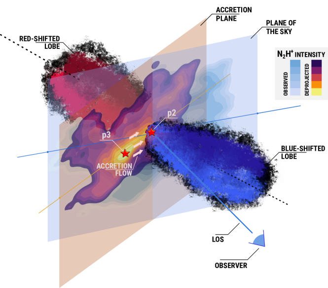
Figure 15: A graphic illustration of the possible 3D configuration that gives raise to the observed structure in Fig. 10. A filamentary structure seen in $\rm N_{2}H^{+}$ (1-0) emission accretes material towards the protostellar core p2. This launches a bipolar outflow likely almost perpendicularly to the accretion flow. The red lobe, when projected on the plane of the sky, appears to coincide with the filament.

To disentangle the complex kinematics shown by the $\rm N_{2}H^{+}$ data and to identify its hierarchical structure in ppv space, we have first fitted the isolated hyperfine component $F_{1}=1-0$ using a three-component Gaussian fit, and then we have used the results as input for the acorns package (Henshaw et al., 2019). The four main trees found by acorns are associated with cores identified in $\rm\text{o-}H_{2}D^{+}$ emission, and at least three host also protostellar cores, suggesting that all of them are active in star formation. One of the trees (labelled B) presents a small velocity gradient ($\approx 1\,$$\rm km\,s^{-1}$ over $0.75\,\rm pc$) and it appears more quiescent than the others, since it contains only one prestellar core. Interestingly, this core (18) is one of those not detected in $\rm N_{2}D^{+}$, which can be explained if it is at an early evolutionary stage, when $\rm N_{2}D^{+}$—a late type molecule— did not have the time yet to form. This tree can then represent a less evolved component with respect to the others in the clump.

The trees labelled A and G are associated with more than 70% of the $\rm\text{o-}H_{2}D^{+}$ cores and three protostellar cores, and they are overlapping and intertwined in ppv space. Such a morphology could be indicative of a sort of competitive accretion scenario, where in the crowded environment of this high-mass clump, multiple low-mass cores ($M_{\mathrm{core}}<30\,\rm M_{\odot}$) have formed. The intraclump gas in which the cores are embedded could provide the cores with the mass reservoir needed to later form high-mass stars. This is also consistent with the fact that at $10\,\rm K$ all the cores are subvirial.

The brightest part of tree G, is structured as a filamentary structure connecting the two protostellar cores p3 and p2. The $\rm N_{2}H^{+}$ centroid velocity increases from $\sim 41\,$$\rm km\,s^{-1}$ close to p3 to $\sim 42\,$$\rm km\,s^{-1}$ close to p2. On the plane of the sky, this structure overlaps with the red lobe of the CO outflow identified by Li et al. (2020). However, the outflow velocities are opposite to that of the $\rm N_{2}H^{+}$ filament, since they are redshifted with respect to the systemic velocity of p2 ($42.8\,$$\rm km\,s^{-1}$). We have speculated on the possibilities that would explain the observed configuration, and we show one of them in Fig. 15. The filamentary structure seen in $\rm N_{2}H^{+}$ emission might be accreting mass onto the protostellar core p2, which then powers a bipolar outflow in a direction likely perpendicular to that of the accretion flow; the red lobe of the bipolar outflow, when seen projected on the plane of the sky, appears overlapped to the $\rm N_{2}H^{+}$ feature, but the two are actually separated in 3D space. Assuming this scenario, we have computed the mass accretion rate along the filamentary structure, obtaining $\dot{M}_{\mathrm{acc}}=2.2\times 10^{-4}\,\rm M_{\odot}\,yr^{-1}$, expected to be accurate within a factor of two, in good agreement with other observations in similar sources. From the outflow parameters, Li et al. (2020) estimated a mass accretion rate on the protostar p2 of $3-4\times 10^{-6}\rm\,M_{\odot}\,yr^{-1}$, i.e. approximately two order of magnitude lower than our estimate, but this value depends on several assumption (for instance on the wind velocity and on the ratio between the mass accretion rate and the mass ejection rate). Furthermore, the value of Li et al. (2020) represents the accretion rate onto the protostar, whilst we compute the rate onto the core.

In this work, we have shown how ALMA observations of several molecular tracers are a powerful diagnostic tool to investigate the fragmentation and kinematic properties of the high-mass clump AG14. In particular, $\rm\text{o-}H_{2}D^{+}$ appears an ideal tracer of the cold and dense gas, and as such it can be used to identify cores likely in an early evolutionary stage. On the other hand, Band 3 data of $\rm N_{2}H^{+}$ can be used to trace the gas kinematics at clump scales and at the clump-to-core transition, providing important information on the dynamics and accretion properties of the gas from which the cores formed.

Appendix A Cores identification in continuum emission

In Sect. 3.1.1 it has been discussed how the morphology of the continuum emission and of the $\rm\text{o-}H_{2}D^{+}$ integrated intensity do not correlate. To strengthen this point, we have performed a core identification also in the dust thermal emission, similarly to what done in Appendix B of Redaelli et al. (2021). We highlight that Sanhueza et al. (2019) already performed a core-finding analysis in the clump, using the continuum data in Band 6, which have a sensitivity $\approx 4$ times higher than the Band 7 data. We however prefer to use the continuum at 0.8 mm to perform the comparison with the $\rm\text{o-}H_{2}D^{+}$ analysis, since these two datasets were observed with the same ALMA configuration.

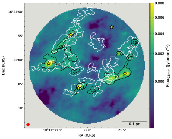
Figure 16: The colorscale show the continuum emission in Band 7. The white contours represent the $\rm\text{o-}H_{2}D^{+}$ cores, whilst the black ones show the cores identified in continuum, which are labelled based on increasing declination. The beam size and scalebar are shown in the bottom left and right corners, respectively. Cores associated with outflow emission according to Li et al. (2020) are shown with stars.

Since scimes works in ppv space, we used the python package astrodendro, on which scimes is based, to analyse the 2D continuum map. Concerning the input parameters necessary to perform the clustering, we set $\Delta_{\mathrm{min}}=1\times rms$ ($rms=0.5\,\rm mJy\,pix^{-1}$ for the non primary-beam corrected map); the minimum value to identify structures is $min_{\mathrm{val}}=2.5\times rms$; the identified cores must be larger that three times the beam size, in order to be consistent with the identification of the $\rm\text{o-}H_{2}D^{+}$ cores.

With these inputs, astrodendro identifies 11 cores, shown in Fig. 16. Four of them (c1, c3, c6, and c11) are found in correspondence with the protostellar candidates. Five cores (22%) seen in $\rm\text{o-}H_{2}D^{+}$ do not correspond to continuum-identified structures, which suggests that they are in a very early stage, and their low temperatures translates in low continuum fluxes at $0.8\,\rm mm$. In turn, continuum core c8 does not overlap with any structure seen in $\rm\text{o-}H_{2}D^{+}(1_{1,0}-1_{1,1})$. This structure corresponds to core 5 in the analysis of Sanhueza et al. (2019) and Li et al. (2020). The latter paper does not consider it as associated with clear outflow emission, even though it shows evidence of CO emission at high velocities. Furthermore, Sanhueza et al. (2019) lists it among the cores with emission from high-energy transitions. It is hence possible that core c8 hosts a young protostar, that either does not power outflow, or that cannot be detected due for instance to projection effects.

Core c3 is the largest one, but it contains three separated flux peaks. It is likely that the algorithm is not able to separate them due to the limited sensitivity of our data. In fact, in Sanhueza et al. (2019) two separated cores were identified in this area in the 1.34 mm continuum emission. In this scenario, core c3 is hence divided in two parts, one which is in a protostellar stage and does not show significant $\rm\text{o-}H_{2}D^{+}$ emission; the other instead is in an earlier evolutionary stage, and it overlaps with several cores seen in $\rm\text{o-}H_{2}D^{+}$. Core c6 is peculiar, in the sense that it overlaps significantly ($>50$%) with $\rm\text{o-}H_{2}D^{+}$ core 1, and it also contains a protostar. As already suggested in Sect. 3.2, these features suggest that this protostar is young, still embedded in a thick envelope that is relatively cold to have a detectable abundance of $\rm\text{o-}H_{2}D^{+}$.

In conclusion, more than half of the $\rm\text{o-}H_{2}D^{+}$ identified cores overlap with continuum cores by less than 30% of their physical extension. This is likely due to different evolutionary stages traced by the two dataset. Whilst the $\rm\text{o-}H_{2}D^{+}$ emission trace cold gas still relatively undisturbed by protostellar activity, the continuum data cannot distinguish between cores in prestellar and protostellar phase. We note that Sanhueza et al. (2019) already identified cores in continuum. We prefer to re-do this analysis, since the Band 6 data used in that paper have a worse resolution (by a factor of $\approx 2.0$) and a larger maximum-recoverable-scale (by $\approx 50$%) that our Band 7 data, and we prefer to analyse a dataset acquired wiith the same interferometer configuration of the $\rm\text{o-}H_{2}D^{+}(1_{1,0}-1_{1,1})$ data. We have however checked that the two methods identifying cores in continuum produce results in reasonable agreement. By comparing the cores found in this appendix and in Sanhueza et al. (2019) (figure not shown here), 10 out of the 11 cores we identify have correspondence to structures seen in Band 6. In the field-of-view where the two datasets overlap, Sanhueza et al. (2019) found more cores, also due to the better sensitivity of their dataset. However, several of the $\rm H_{2}D^{+}$-identified cores (5 out of 22) still have no clear correspondence with continuum-identified structures, and our conclusion that continuum and line morfologies are different still holds.

Appendix B Results of the spectral fit of the $\rm\text{o-}H_{2}D^{+}(1_{1,0}-1_{1,1})$ transition in each core

Figs. 17 to 20 present the maps of the best-fit parameters obtained with mcweeds in each core. Concerning the linewidths, here we show the $FWHM$ maps, which is the actual free parameter used in the fitting procedure.

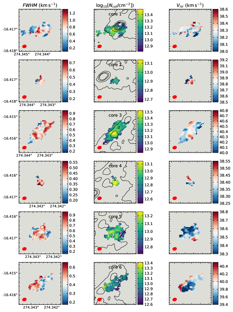
Figure 17: Maps of best-fit parameters obtained with mcweeds. The columns are $FWHM$, $N_{\mathrm{col}}$, and $V_{\mathrm{lsr}}$, from left to right. The core label is indicated at the top of each central panel. The contours show the continuum emission at levels from $2$ to $11\sigma$, in steps of $3\sigma$.

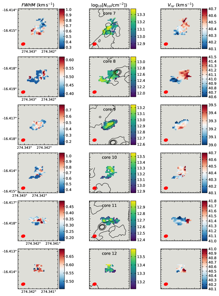
Figure 18: Continuation of Fig. 17.

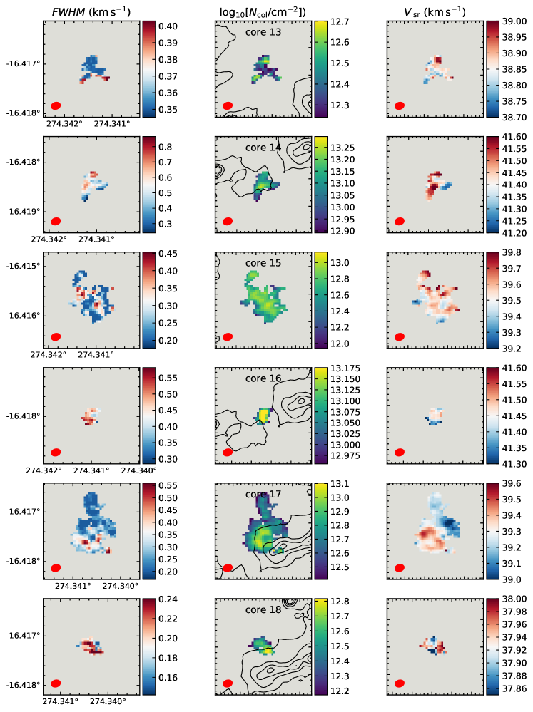
Figure 19: Continuation of Fig. 17.

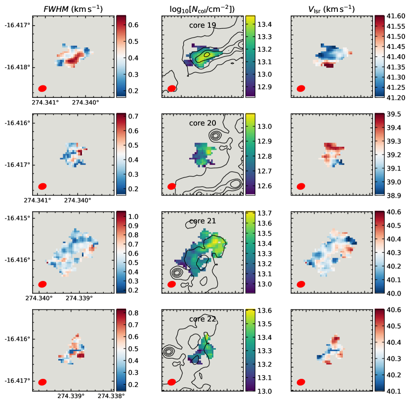
Figure 20: Continuation of Fig. 17.

Appendix C Opacity and missing flux of the $\rm\text{o-}H_{2}D^{+}(1_{1,0}-1_{1,1})$ line

In order to estimate the opacity of the $\rm\text{o-}H_{2}D^{+}(1_{1,0}-1_{1,1})$ line, we make use of the equation:

$$\tau_{\nu}=-\ln{1-\frac{T_{\mathrm{b}}}{J_{\nu}(T_{\mathrm{ex}})-J_{\nu}(T_{\mathrm{bg}})}}\;,$$ (C1)

where $J_{\nu}(T)$ is the equivalent Rayleigh-Jeans temperature at the frequency $\nu$ and temperature $T$, and $T_{\mathrm{bg}}=2.73\rm\,K$ is the background temperature. In the ALMA data, the brightness temperature peaks at $2\,\rm K$. Using $\text{$T_{\mathrm{ex}}$}=10\,\rm K$, Eq. C1 yields $\tau_{\nu}\approx 0.8$. Even in the brightest part of the emission, hence, the line is only moderately optically thick. With this information, we can also estimate by how much the linewidths would be overestimated towards the positions of the source with the highest optical depth. To do so, we make use of Eq. 52 of Burton et al. (1992):

$$\sigma_{\mathrm{obs}}=\frac{\sigma_{0}}{\sqrt{\ln(2)}}\left\{\ln\left[\frac{\tau_{\nu}}{\ln\left(\frac{2}{1+e^{-\tau_{\nu}}}\right)}\right]\right\}^{\frac{1}{2}}\;,$$ (C2)

which allows to infer the observed velocity dispersion $\sigma_{\mathrm{obs}}$ from the intrinsic one $\sigma_{0}$ given the line opacity $\tau_{\nu}$. Using the maximum value for the opacity just found, we estimate that in the most optically thick parts of the source the $\rm\text{o-}H_{2}D^{+}(1_{1,0}-1_{1,1})$ linewidth is overestimated by 15% .

The ALMA Band 7 data lack of Total Power observations, which is crucial to recover the large-scale emission from the source. In order to quantify if and how the observations are affected by filtering-out, we compare the $\rm\text{o-}H_{2}D^{+}(1_{1,0}-1_{1,1})$ spectra observed with the APEX single-dish telescope towards AG14 (Sabatini et al., 2020) with the ALMA data in Fig. 21. The APEX data have been converted in flux unit using the gain $G_{\mathrm{APEX}}=40\,\rm Jy\,K^{-1}$. The ALMA data instead have been integrated over an area equal to the beam size of the single-dish ($\theta_{\mathrm{APEX}}=16^{\prime\prime}.8$), and smoothed to the same spectral resolution.

Figure 21 shows that the interferometer is recovering only $\sim$ one fifth of the emission. The missing flux arises from the large scales, since the emission is more extended that the maximum recoverable scale of the telescope in this configuration ($\theta_{\mathrm{MRS}}\approx 20^{\prime\prime}$, as was already noted for AG351 and AG354 in Redaelli et al. (2021). However, the ALMA data do not usually present anomalous line shapes. Furthermore, the core identified by scimes are significantly smaller than $\theta_{\mathrm{MRS}}\approx 20^{\prime\prime}$. We hence conclude that the missing flux problem does not affect significantly the analysis of the present work.

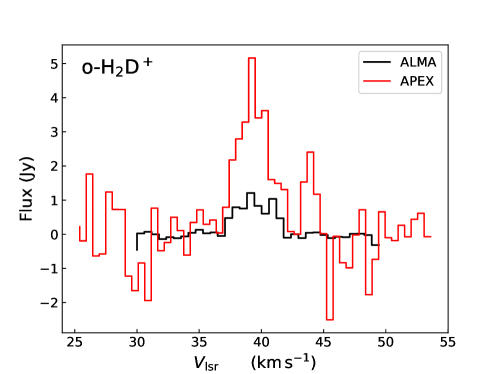
Figure 21: Comparison of the $\rm\text{o-}H_{2}D^{+}(1_{1,0}-1_{1,1})$ spectra obtained towards AG14 with the APEX single-dish telescope (red histogram) and the ALMA interferometer (black histogram). See the text for the technical details about how the spectra have been extracted.

Appendix D $\rm N_{2}H^{+}$ fitting and full results of acorns clustering

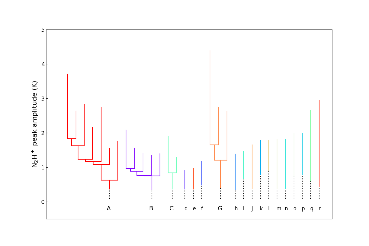
Figure 22: Results of the acorns clustering algorithm run on the results of the multi-component Gaussian fitting of the $\rm N_{2}H^{+}$ (1-0) transition, shown graphically as a dendrogram. The different colours represent distinct trees, labelled with letters, and they correspond to the structures shown in Fig. 23. The four trees labelled with capital letters contain more than 70% of all data, and 80% of the total flux.

The multi-component Gaussian fit of the $\rm N_{2}H^{+}$ isolated hyperfine transition, performed with the pyspeckit package, have nine free parameters in total: $V_{\mathrm{lsr}}$, $\sigma_{\mathrm{V}}$, and $T_{\mathrm{peak}}$ values, times three Gaussian components. To improve the code convergence, we first masked pixels with $\rm S/N<10$ in peak intensity. This choice leaves 5387 positions (55% of the total) unmasked, which however still cover the whole $\rm\text{o-}H_{2}D^{+}$ FoV. We limited the space of the parameters as follows: $V_{\mathrm{lsr}}\in[36;43]$$\rm km\,s^{-1}$; $T_{\mathrm{peak}}>0\,$K; $\sigma_{\mathrm{V}}\in[0;2.5]$$\rm km\,s^{-1}$. Due to the large gradients of the free parameters over the map, the fitting routine does not converge everywhere. After a first procedure, we hence selected the spectra with residuals $>2\sigma$ ($1\sigma=120\,\rm mK$; the $rms$ of the residuals is computed in the velocity range $[34.6;43.5]$$\rm km\,s^{-1}$), and we performed a second fit, adjusting the initial guesses on the free parameters. We checked the residuals after this second fitting routine, and their $rms$ is found to be $<3\sigma$. We further masked pixel-per-pixel velocity components for which the fit did not converge, or with large uncertainties (e.g. $\sigma_{T_{\mathrm{peak}}}>1\,$K).

The best-fit results of the Gaussian fitting routine are fed to the clustering alorithm acorns. Unlike other similar codes, acorns uses the spectra linewidth as a further parameter to build the cluster hierarchy, and it is overall able to distinguish structures overlapping in ppv space better than other algorithms, which turns helpful for the crowded kinematics of AG14 (see also Appendix B in Henshaw et al. 2019 for further details on the comparison between different algorithms). We select the following clustering criteria in acorns:

1. Clusters must have a minimum size of 1.5 ALMA beam (to ensure that all the structures found are marginally resolved);

2. They must be separated in velocity less than spectral resolution of the data-cube;

3. The maximum separation in velocity dispersion ($FWHM$) is less than the gas thermal velocity at 10$\,\rm K$ ($0.19\,$$\rm km\,s^{-1}$);

4. The minimum height of an independent cluster is $3\sigma$, and the stop criteria is set to $5\sigma$ ($1\sigma=0.12\,\rm K$).

After a first run, the code performs a second cycle of clustering, when we relax the criteria by 30%, which further helps building the hierarchical structure according to the prescriptions of acorns. At the end, the algorithm is able to cluster 87% of the data-points, and it finds 18 trees, shown in Fig. 22 as a dendrogram, and in Fig. 23 in ppv space. The large majority (more than 70%) of clustered data-points belongs to only four structures, which also contain $\approx 80$% of the total flux (A, B, C, and G as labelled in Fig. 22). The remaining clusters contain less than 3% of the data-points each. The analysis of Sect. 3.2 hence focuses on these four trees.

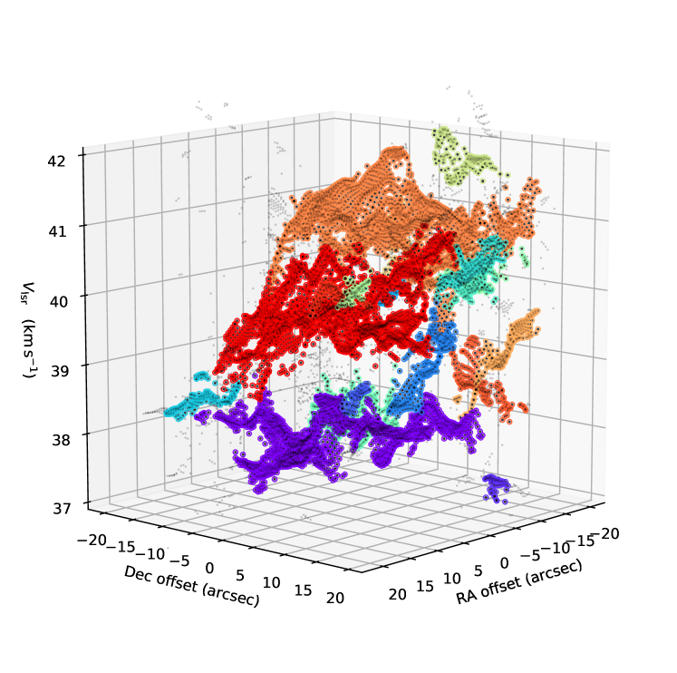
Figure 23: Ppv diagram with the complete set of trees identified by acorns. The coordinates axes are expressed as offsets (in arcsec) with respect to the position $\text{RA}=\rm 18^{h}17^{m}22.0^{s}$, $\rm Dec=-16\text{\degree}25^{\prime}01^{\prime\prime}.7$. Each colour represent a different tree, and have correspondence in the dendrogram shown in Fig. 22. Grey points do not belong to any cluster.

We now discuss why we prefer to use distinct softwares to analyse the $\rm N_{2}H^{+}$ and $\rm\text{o-}H_{2}D^{+}$ data. scimes is optimise to work with low-to-medium S/N data, such as the $\rm\text{o-}H_{2}D^{+}$ ones. Furthermore, using it ensures a proper comparison with the results of Redaelli et al. (2021), which in turn allows to obtain a larger sample for instance regarding the core masses. acorns, on the other hand, represents a better choice to analyse the $\rm N_{2}H^{+}$ data, first of all because it has less problems to disentangle crowded spectra such as the ones in AG14. scimes in fact works on the observed ppv datacubes, and it performs better when the multiple velocity components are well separated in velocity space, as in the $\rm\text{o-}H_{2}D^{+}$ data, where these components are separated by $\approx~{}1\,$$\rm km\,s^{-1}$ and they are narrow ($\sigma_{\mathrm{V}}=0.3\,$$\rm km\,s^{-1}$). On the contrary, the $\rm N_{2}H^{+}$ spectra are more crowded, with more velocity components, and some of these components have significantly broader lines ($\sigma_{\mathrm{V}}=0.6-1.0\,$$\rm km\,s^{-1}$). Due to these features, scimes is not able to disentangle them, as demonstrated by a test run of the software that we performed on the $\rm N_{2}H^{+}$ datacube. acorns instead is able to perform this task because it works on decomposed data. There is also another important difference, in that acorns performs the clustering also in velocity dispersion space. The $\rm\text{o-}H_{2}D^{+}(1_{1,0}-1_{1,1})$ linewidths span a much smaller range ($\approx 0.2-0.4\,$$\rm km\,s^{-1}$) with respect to the $\rm N_{2}H^{+}$ ones ($\approx 0.3-1.5\,$$\rm km\,s^{-1}$), and therefore this extra constraint helps even more in disentangling the $\rm N_{2}H^{+}$ complex kinematics.

References

- Arzoumanian et al. (2011) Arzoumanian, D., André, P., Didelon, P., et al. 2011, A&A, 529, L6, doi: 10.1051/0004-6361/201116596
- Arzoumanian et al. (2019) Arzoumanian, D., André, P., Könyves, V., et al. 2019, A&A, 621, A42, doi: 10.1051/0004-6361/201832725
- Bacmann et al. (2002) Bacmann, A., Lefloch, B., Ceccarelli, C., et al. 2002, A&A, 389, L6, doi: 10.1051/0004-6361:20020652
- Baldeschi et al. (2017) Baldeschi, A., Elia, D., Molinari, S., et al. 2017, MNRAS, 466, 3682, doi: 10.1093/mnras/stw3353
- Barnes et al. (2018) Barnes, A. T., Henshaw, J. D., Caselli, P., et al. 2018, MNRAS, 475, 5268, doi: 10.1093/mnras/sty173
- Beckwith et al. (1990) Beckwith, S. V. W., Sargent, A. I., Chini, R. S., & Guesten, R. 1990, AJ, 99, 924, doi: 10.1086/115385
- Bertoldi & McKee (1992) Bertoldi, F., & McKee, C. F. 1992, ApJ, 395, 140, doi: 10.1086/171638
- Bonnell & Bate (2006) Bonnell, I. A., & Bate, M. R. 2006, MNRAS, 370, 488, doi: 10.1111/j.1365-2966.2006.10495.x
- Bonnell et al. (2001) Bonnell, I. A., Bate, M. R., Clarke, C. J., & Pringle, J. E. 2001, MNRAS, 323, 785, doi: 10.1046/j.1365-8711.2001.04270.x
- Burton et al. (1992) Burton, W. B., Elmegreen, B. G., Genzel, R., et al. 1992, Saas-Fee Advanced Course 21: The Galactic Interstellar Medium
- Caselli et al. (2008) Caselli, P., Vastel, C., Ceccarelli, C., et al. 2008, A&A, 492, 703, doi: 10.1051/0004-6361:20079009
- Caselli et al. (1999) Caselli, P., Walmsley, C. M., Tafalla, M., Dore, L., & Myers, P. C. 1999, ApJ, 523, L165, doi: 10.1086/312280
- Ceccarelli et al. (2014) Ceccarelli, C., Caselli, P., Bockelée-Morvan, D., et al. 2014, in Protostars and Planets VI, ed. H. Beuther, R. S. Klessen, C. P. Dullemond, & T. Henning, 859, doi: 10.2458/azu_uapress_9780816531240-ch037
- Chen et al. (2019) Chen, H.-R. V., Zhang, Q., Wright, M. C. H., et al. 2019, ApJ, 875, 24, doi: 10.3847/1538-4357/ab0f3e
- Colombo et al. (2015) Colombo, D., Rosolowsky, E., Ginsburg, A., Duarte-Cabral, A., & Hughes, A. 2015, MNRAS, 454, 2067, doi: 10.1093/mnras/stv2063
- Contreras et al. (2018) Contreras, Y., Sanhueza, P., Jackson, J. M., et al. 2018, ApJ, 861, 14, doi: 10.3847/1538-4357/aac2ec
- Cornwell (2008) Cornwell, T. J. 2008, IEEE Journal of Selected Topics in Signal Processing, 2, 793, doi: 10.1109/JSTSP.2008.2006388
- Fontani et al. (2021) Fontani, F., Barnes, A. T., Caselli, P., et al. 2021, MNRAS, 503, 4320, doi: 10.1093/mnras/stab700
- Friesen et al. (2014) Friesen, R. K., Di Francesco, J., Bourke, T. L., et al. 2014, ApJ, 797, 27, doi: 10.1088/0004-637X/797/1/27
- Giannetti et al. (2017) Giannetti, A., Leurini, S., Wyrowski, F., et al. 2017, A&A, 603, A33, doi: 10.1051/0004-6361/201630048
- Giannetti et al. (2014) Giannetti, A., Wyrowski, F., Brand, J., et al. 2014, A&A, 570, A65, doi: 10.1051/0004-6361/201423692
- Giannetti et al. (2019) Giannetti, A., Bovino, S., Caselli, P., et al. 2019, A&A, 621, L7, doi: 10.1051/0004-6361/201834602
- Ginsburg & Mirocha (2011) Ginsburg, A., & Mirocha, J. 2011, PySpecKit: Python Spectroscopic Toolkit, Astrophysics Source Code Library, record ascl:1109.001. http://ascl.net/1109.001
- Goldsmith (2001) Goldsmith, P. F. 2001, ApJ, 557, 736, doi: 10.1086/322255
- Guzmán et al. (2015) Guzmán, A. E., Sanhueza, P., Contreras, Y., et al. 2015, ApJ, 815, 130, doi: 10.1088/0004-637X/815/2/130
- Hacar et al. (2022) Hacar, A., Clark, S., Heitsch, F., et al. 2022, arXiv e-prints, arXiv:2203.09562. https://arxiv.org/abs/2203.09562
- Henshaw et al. (2014) Henshaw, J. D., Caselli, P., Fontani, F., Jiménez-Serra, I., & Tan, J. C. 2014, MNRAS, 440, 2860, doi: 10.1093/mnras/stu446
- Henshaw et al. (2019) Henshaw, J. D., Ginsburg, A., Haworth, T. J., et al. 2019, MNRAS, 485, 2457, doi: 10.1093/mnras/stz471
- Hildebrand (1983) Hildebrand, R. H. 1983, QJRAS, 24, 267
- Hugo et al. (2009) Hugo, E., Asvany, O., & Schlemmer, S. 2009, J. Chem. Phys., 130, 164302, doi: 10.1063/1.3089422
- Jusko et al. (2017) Jusko, P., Töpfer, M., Müller, H. S. P., et al. 2017, Journal of Molecular Spectroscopy, 332, 33, doi: 10.1016/j.jms.2016.09.013
- Kauffmann et al. (2008) Kauffmann, J., Bertoldi, F., Bourke, T. L., Evans, N. J., I., & Lee, C. W. 2008, A&A, 487, 993, doi: 10.1051/0004-6361:200809481
- Kauffmann & Pillai (2010) Kauffmann, J., & Pillai, T. 2010, ApJ, 723, L7, doi: 10.1088/2041-8205/723/1/L7
- Kauffmann et al. (2013) Kauffmann, J., Pillai, T., & Goldsmith, P. F. 2013, ApJ, 779, 185, doi: 10.1088/0004-637X/779/2/185
- Koch & Rosolowsky (2015) Koch, E. W., & Rosolowsky, E. W. 2015, MNRAS, 452, 3435, doi: 10.1093/mnras/stv1521
- König et al. (2017) König, C., Urquhart, J. S., Csengeri, T., et al. 2017, A&A, 599, A139, doi: 10.1051/0004-6361/201526841
- Krumholz & McKee (2008) Krumholz, M. R., & McKee, C. F. 2008, Nature, 451, 1082, doi: 10.1038/nature06620
- Kuiper et al. (2016) Kuiper, R., Turner, N. J., & Yorke, H. W. 2016, ApJ, 832, 40, doi: 10.3847/0004-637X/832/1/40
- Li et al. (2019) Li, S., Zhang, Q., Pillai, T., et al. 2019, ApJ, 886, 130, doi: 10.3847/1538-4357/ab464e
- Li et al. (2020) Li, S., Zhang, Q., Liu, H. B., et al. 2020, ApJ, 896, 110, doi: 10.3847/1538-4357/ab84f1
- Li et al. (2020) Li, S., Sanhueza, P., Zhang, Q., et al. 2020, ApJ, 903, 119, doi: 10.3847/1538-4357/abb81f
- Li et al. (2022) Li, S., Sanhueza, P., Lee, C. W., et al. 2022, ApJ, 926, 165, doi: 10.3847/1538-4357/ac3df8
- Lu et al. (2018) Lu, X., Zhang, Q., Liu, H. B., et al. 2018, ApJ, 855, 9, doi: 10.3847/1538-4357/aaad11
- MacLaren et al. (1988) MacLaren, I., Richardson, K. M., & Wolfendale, A. W. 1988, ApJ, 333, 821, doi: 10.1086/166791
- Maret et al. (2011) Maret, S., Hily-Blant, P., Pety, J., Bardeau, S., & Reynier, E. 2011, A&A, 526, A47, doi: 10.1051/0004-6361/201015487
- McKee & Tan (2003) McKee, C. F., & Tan, J. C. 2003, ApJ, 585, 850, doi: 10.1086/346149
- McMullin et al. (2007) McMullin, J. P., Waters, B., Schiebel, D., Young, W., & Golap, K. 2007, in Astronomical Society of the Pacific Conference Series, Vol. 376, Astronomical Data Analysis Software and Systems XVI, ed. R. A. Shaw, F. Hill, & D. J. Bell, 127
- Mezger et al. (1990) Mezger, P. G., Wink, J. E., & Zylka, R. 1990, A&A, 228, 95
- Morii et al. (2021) Morii, K., Sanhueza, P., Nakamura, F., et al. 2021, ApJ, 923, 147, doi: 10.3847/1538-4357/ac2365
- Myers et al. (1991) Myers, P. C., Ladd, E. F., & Fuller, G. A. 1991, ApJ, 372, L95, doi: 10.1086/186032
- Ohashi et al. (2016) Ohashi, S., Sanhueza, P., Chen, H.-R. V., et al. 2016, ApJ, 833, 209, doi: 10.3847/1538-4357/833/2/209
- Ostriker (1964) Ostriker, J. 1964, ApJ, 140, 1056, doi: 10.1086/148005
- Palmeirim et al. (2013) Palmeirim, P., André, P., Kirk, J., et al. 2013, A&A, 550, A38, doi: 10.1051/0004-6361/201220500
- Patil et al. (2010) Patil, A., Huard, D., & Fonnesbeck, C. J. 2010, Journal of Statistical Software, Articles, 35, 1, doi: 10.18637/jss.v035.i04
- Peretto et al. (2014) Peretto, N., Fuller, G. A., André, P., et al. 2014, A&A, 561, A83, doi: 10.1051/0004-6361/201322172
- Pillai et al. (2019) Pillai, T., Kauffmann, J., Zhang, Q., et al. 2019, A&A, 622, A54, doi: 10.1051/0004-6361/201732570
- Pon et al. (2012) Pon, A., Toalá, J. A., Johnstone, D., et al. 2012, ApJ, 756, 145. doi:10.1088/0004-637X/756/2/145
- Rathborne et al. (2006) Rathborne, J. M., Jackson, J. M., & Simon, R. 2006, ApJ, 641, 389, doi: 10.1086/500423
- Redaelli et al. (2021) Redaelli, E., Bovino, S., Giannetti, A., et al. 2021, A&A, 650, A202, doi: 10.1051/0004-6361/202140694
- Rosolowsky & Leroy (2006) Rosolowsky, E., & Leroy, A. 2006, PASP, 118, 590, doi: 10.1086/502982
- Rosolowsky et al. (2008) Rosolowsky, E. W., Pineda, J. E., Kauffmann, J., & Goodman, A. A. 2008, ApJ, 679, 1338, doi: 10.1086/587685
- Sabatini et al. (2019) Sabatini, G., Giannetti, A., Bovino, S., et al. 2019, MNRAS, 490, 4489, doi: 10.1093/mnras/stz2818
- Sabatini et al. (2020) Sabatini, G., Bovino, S., Giannetti, A., et al. 2020, A&A, 644, A34, doi: 10.1051/0004-6361/202039010
- Sabatini et al. (2022) Sabatini, G., Bovino, S., Sanhueza, P., et al. 2022, arXiv:2207.12431
- Sakai et al. (2022) Sakai, T., Sanhueza, P., Furuya, K., et al. 2022, ApJ, 925, 144, doi: 10.3847/1538-4357/ac3d2e
- Sanhueza et al. (2012) Sanhueza, P., Jackson, J. M., Foster, J. B., et al. 2012, ApJ, 756, 60, doi: 10.1088/0004-637X/756/1/60
- Sanhueza et al. (2013) —. 2013, ApJ, 773, 123, doi: 10.1088/0004-637X/773/2/123
- Sanhueza et al. (2017) Sanhueza, P., Jackson, J. M., Zhang, Q., et al. 2017, ApJ, 841, 97, doi: 10.3847/1538-4357/aa6ff8
- Sanhueza et al. (2019) Sanhueza, P., Contreras, Y., Wu, B., et al. 2019, ApJ, 886, 102, doi: 10.3847/1538-4357/ab45e9
- Sanhueza et al. (2021) Sanhueza, P., Girart, J. M., Padovani, M., et al. 2021, ApJ, 915, L10, doi: 10.3847/2041-8213/ac081c
- Shirley (2015) Shirley, Y. L. 2015, PASP, 127, 299, doi: 10.1086/680342
- Singh et al. (2021) Singh, A., Matzner, C. D., Friesen, R. K., et al. 2021, ApJ, 922, 87, doi: 10.3847/1538-4357/ac20d2
- Sipilä et al. (2013) Sipilä, O., Caselli, P., & Harju, J. 2013, A&A, 554, A92, doi: 10.1051/0004-6361/201220922
- Sipilä et al. (2015) —. 2015, A&A, 578, A55, doi: 10.1051/0004-6361/201424364
- Smith et al. (2009) Smith, R. J., Longmore, S., & Bonnell, I. 2009, MNRAS, 400, 1775, doi: 10.1111/j.1365-2966.2009.15621.x
- Sokolov et al. (2019) Sokolov, V., Wang, K., Pineda, J. E., et al. 2019, ApJ, 872, 30, doi: 10.3847/1538-4357/aafaff
- Svoboda et al. (2019) Svoboda, B. E., Shirley, Y. L., Traficante, A., et al. 2019, ApJ, 886, 36, doi: 10.3847/1538-4357/ab40ca
- Tafoya et al. (2021) Tafoya, D., Sanhueza, P., Zhang, Q., et al. 2021, ApJ, 913, 131, doi: 10.3847/1538-4357/abf5da
- Tan et al. (2014) Tan, J. C., Beltrán, M. T., Caselli, P., et al. 2014, in Protostars and Planets VI, ed. H. Beuther, R. S. Klessen, C. P. Dullemond, & T. Henning, 149, doi: 10.2458/azu_uapress_9780816531240-ch007
- Tan et al. (2013) Tan, J. C., Kong, S., Butler, M. J., Caselli, P., & Fontani, F. 2013, ApJ, 779, 96, doi: 10.1088/0004-637X/779/2/96
- Tan et al. (2016) Tan, J. C., Kong, S., Zhang, Y., et al. 2016, ApJ, 821, L3, doi: 10.3847/2041-8205/821/1/L3
- Toalá et al. (2012) Toalá, J. A., Vázquez-Semadeni, E., & Gómez, G. C. 2012, ApJ, 744, 190, doi: 10.1088/0004-637X/744/2/190
- Walker et al. (1990) Walker, C. K., Adams, F. C., & Lada, C. J. 1990, ApJ, 349, 515, doi: 10.1086/168338
- Wang et al. (2020) Wang, J.-W., Koch, P. M., Galván-Madrid, R., et al. 2020, ApJ, 905, 158, doi: 10.3847/1538-4357/abc74e
- Wang et al. (2010) Wang, P., Li, Z.-Y., Abel, T., & Nakamura, F. 2010, ApJ, 709, 27, doi: 10.1088/0004-637X/709/1/27
- Williams et al. (2018) Williams, G. M., Peretto, N., Avison, A., Duarte-Cabral, A., & Fuller, G. A. 2018, A&A, 613, A11, doi: 10.1051/0004-6361/201731587
- Zhang et al. (2015) Zhang, Q., Wang, K., Lu, X., & Jiménez-Serra, I. 2015, ApJ, 804, 141, doi: 10.1088/0004-637X/804/2/141