Weakly-Supervised Camouflaged Object Detection with Scribble Annotations

Abstract

Existing camouflaged object detection (COD) methods rely heavily on large-scale datasets with pixel-wise annotations. However, due to the ambiguous boundary, annotating camouflage objects pixel-wisely is very time-consuming and labor-intensive, taking $\sim$60mins to label one image. In this paper, we propose the first weakly-supervised COD method, using scribble annotations as supervision. To achieve this, we first relabel 4,040 images in existing camouflaged object datasets with scribbles, which takes $\sim$10s to label one image. As scribble annotations only describe the primary structure of objects without details, for the network to learn to localize the boundaries of camouflaged objects, we propose a novel consistency loss composed of two parts: a cross-view loss to attain reliable consistency over different images, and an inside-view loss to maintain consistency inside a single prediction map. Besides, we observe that humans use semantic information to segment regions near the boundaries of camouflaged objects. Hence, we further propose a feature-guided loss, which includes visual features directly extracted from images and semantically significant features captured by the model. Finally, we propose a novel network for COD via scribble learning on structural information and semantic relations. Our network has two novel modules: the local-context contrasted (LCC) module, which mimics visual inhibition to enhance image contrast/sharpness and expand the scribbles into potential camouflaged regions, and the logical semantic relation (LSR) module, which analyzes the semantic relation to determine the regions representing the camouflaged object. Experimental results show that our model outperforms relevant SOTA methods on three COD benchmarks with an average improvement of 11.0$\%$ on MAE, 3.2$\%$ on S-measure, 2.5$\%$ on E-measure, and 4.4$\%$ on weighted F-measure.

Introduction

Camouflaged object detection (COD) aims to detect visually inconspicuous objects in their surroundings, which includes natural objects with protective coloring, small sizes, occlusion, and artificial objects with information hiding purposes. Ambiguous boundaries between objects and backgrounds make it a more challenging task than other object detection tasks. Drawing increasing attention from the computer vision community, COD have numerous promising applications, including species discovery (Pérez-de la Fuente et al. 2012), medical image segmentation (like polyp segmentation with indistinguishable lesions) (Fan et al. 2020c, b), and animal-search (Fan et al. 2021).

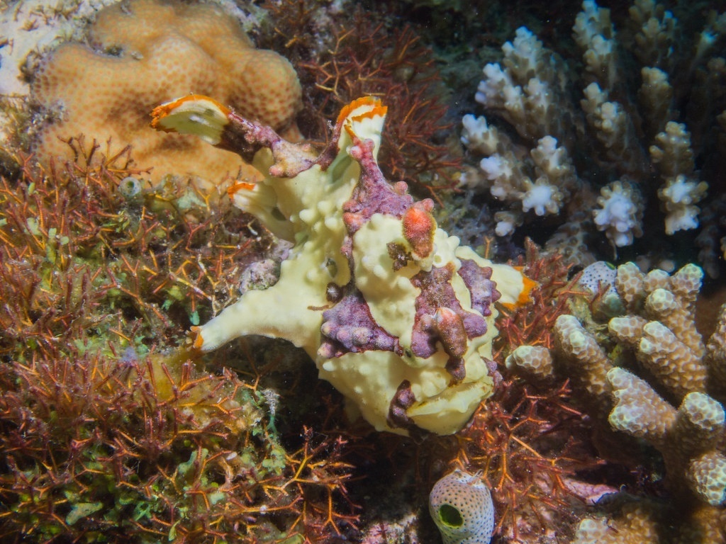
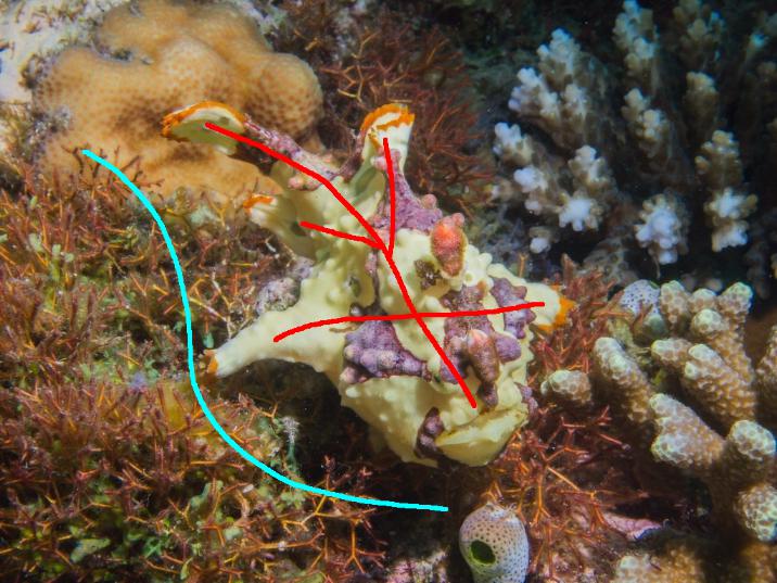
Input GT (pixel-wise) Scribble

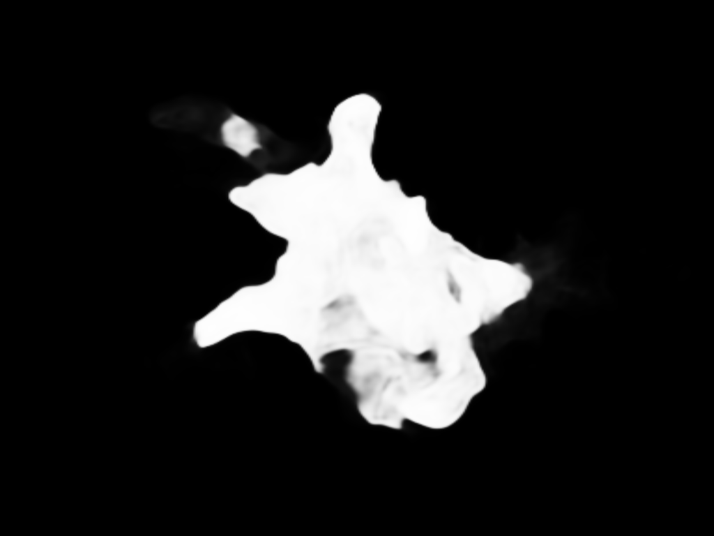
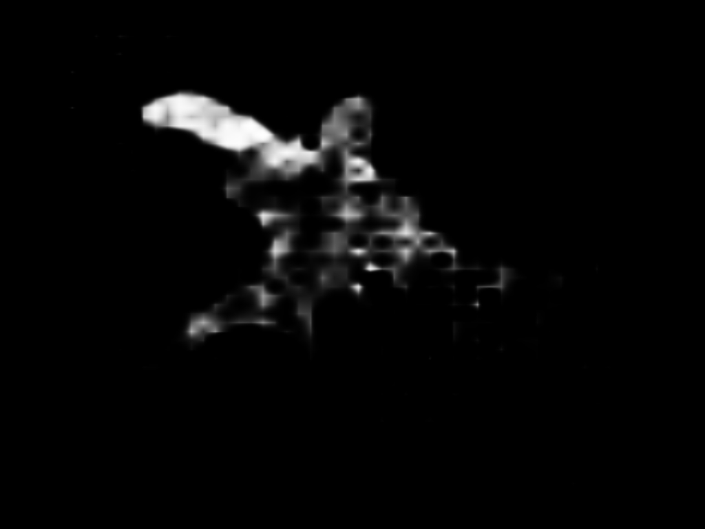
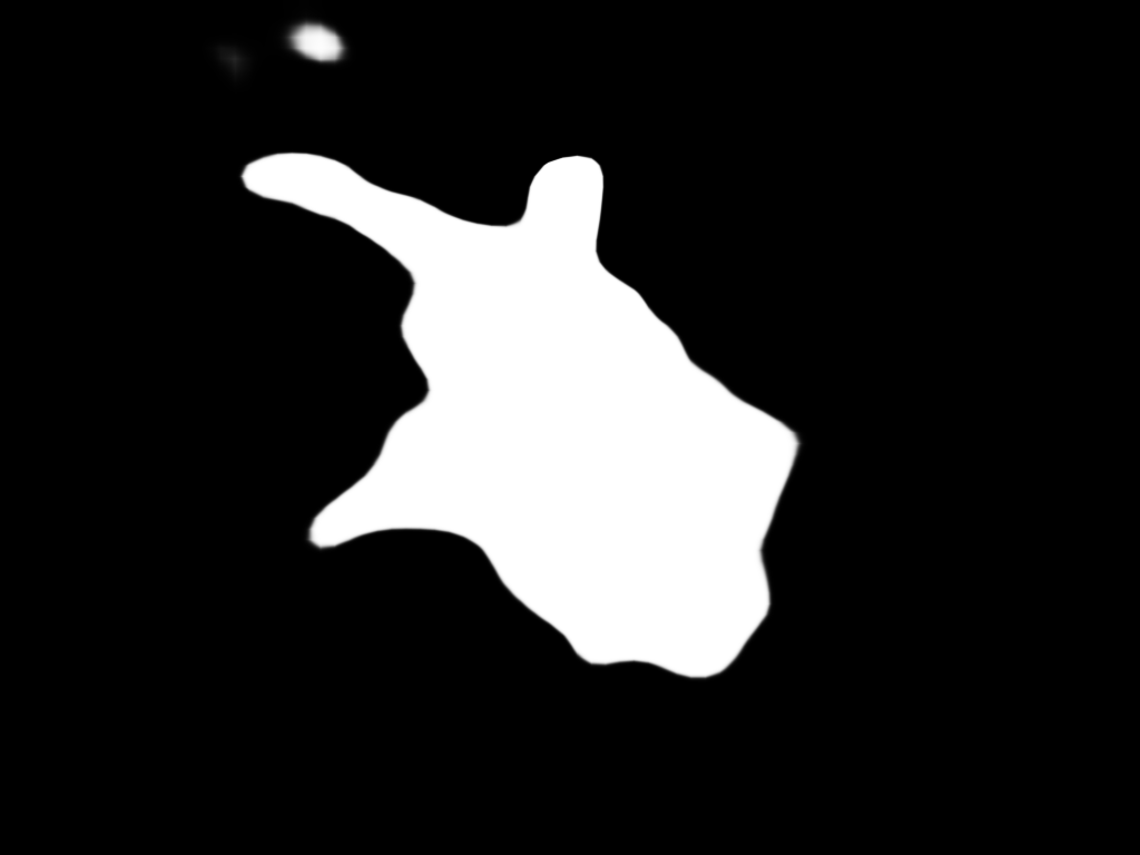
ZoomNet UGTR Ours

Figure 1: Scribbles only indicate the primary structure of objects (cyan for background, red for foreground). Our method exploits this property to effectively learn rich semantic and structural information from the sparse labels. In some cases, it performs even better than fully-supervised models (Youwei et al. 2022; Yang et al. 2021).

Although COD methods have already achieved excellent performances, they rely heavily on pixel-wise annotations of large-scale datasets. There are two main weaknesses of pixel-wise annotations. First, they are time-consuming. It takes $\sim$60 minutes to annotate one image (Fan et al. 2020a), which makes it very laborious to construct large-scale datasets. In contrast, according to our experience, scribble annotation only costs $\sim$10 seconds, which is 360 times faster than pixel-wise annotation. Second, pixel-wise annotation assigns equal significance to each object pixel, which may cause the model to fail in learning primary structures, as shown in the second row of Figure 1. To address these problems, we propose the first scribble-based COD dataset, named S-COD. It contains 3,040 images from the training set of COD10K (Fan et al. 2020a) and 1,000 images from the training set of CAMO (Le et al. 2019). Annotators are asked to scribble the primary structure according to their first impressions without knowing the ground-truth. Figure 2 shows the percentage of annotated pixels in S-COD. Compared to pixel-wise annotation, the labeling process of S-COD is much easier. Compared with other labeling approaches (e.g., box and point annotation), it provides more pixel-level guidance, allowing semantic information to be exploited, and is comparably efficient in labeling.

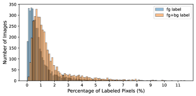
Figure 2: Percentage of labeled pixels in the S-COD dataset.

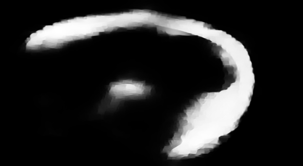
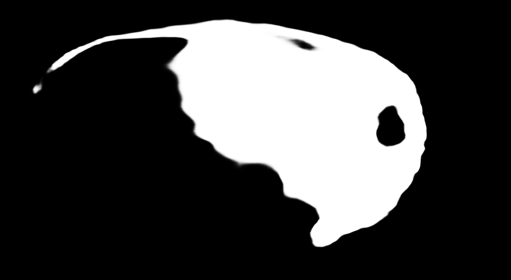
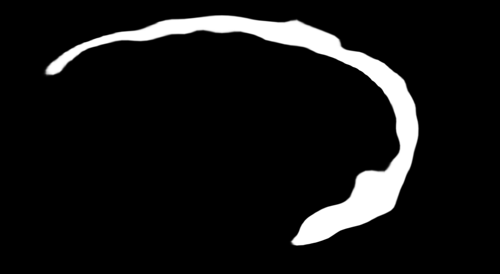
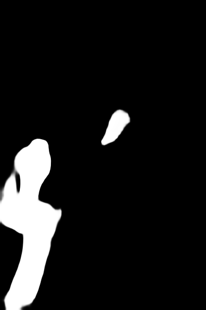
Input GT SS SCWSSOD Ours

Figure 3: Two popular scenarios where existing scribble-supervised SOD methods SS (Zhang et al. 2020b) and SCWSSOD (Yu et al. 2021) fail to exploit semantic features.

Nevertheless, how to exploit scribble annotations for COD is still under exploration. Directly applying existing scribble-based salient object detection (SOD) methods are not appropriate here since camouflaged objects are not salient. Figure 3 shows that two state-of-the-art scribble-based SOD methods, SS (Zhang et al. 2020b) and SCWSSOD (Yu et al. 2021), fail in two common scenarios. The first row of Figure 3 shows an object with an ambiguous boundary in the generally consistent background. Due to the similar low-level features, both SS and SCWSSOD experience difficulties recognizing the boundaries. The second row requires detectors to identify semantic relations of objects (e.g., flower stems and petals), as more than one object looks like the “camouflaged” foreground. Here, both SS and SCWSSOD mistakenly include other objects as the foreground, due to poor semantic information learning.

In this paper, we present the first scribble-based COD learning framework to address the weakly-supervised COD problem with scribble annotations. We observe that humans would first identify possible foreground objects (Wald 1935) and then use semantic information to exactly segment them (Hubel and Wiesel 1962). To incorporate this process in our model, we propose a feature-guided loss, which considers not only visual affinity but also high-level semantic features, to guide the segmentation. The high-level features are learned in an end-to-end fashion during training and do not depend on other well-trained detectors. In addition, in our network design, we propose the local-context contrasted (LCC) module to mimick visual inhibition in strengthening contrast (Von Békésy 2017) in order to find potential camouflaged regions, and the logical semantic relation (LSR) module to determine the final camouflaged object regions. Further, we notice that current weakly-supervised methods tend to have inconsistent predictions in COD, possibly due to the “camouflage” characteristics. Hence, we design a consistency regularization, which is stronger and more reliable than previous weakly-supervised learning methods. Specifically, we introduce the reliability bias in the cross-view loss to improve the self-consistency mechanism. We also present the inside-view consistency loss to reduce the uncertainty of predictions. The regularization enhances the stability and quality of the prediction.

In conclusion, our main contributions are as follows:

• We propose the first weakly-supervised COD dataset with scribble annotation. Compared with pixel-wise annotation, it takes only $\sim$10 seconds to annotate each image (360 times faster) and overcomes the limitation of assigning equal importance to every object pixel.

• We propose the first end-to-end weakly-supervised COD framework. It includes novel feature-guided loss functions and consistency loss. Imitating human perceptions, the loss functions guide the network to extract high-level features that help distinguish objects and impose stability on the predictions.

• We propose a novel network for scribble learning, which utilizes low-level contrasts to expand the scribbles to wider camouflaged regions and logical semantic information to finalize the objects.

• Experimental results show that our framework outperforms relevant state-of-the-art methods on three COD benchmarks with an average improvement of 11.0$\%$ on MAE, 3.2$\%$ on S-measure, 2.5$\%$ on E-measure, and 4.4$\%$ on weighted F-measure.

Related Work

Camouflaged Object Detection. COD focuses on undetectable natural objects (e.g., hidden objects, tiny objects, objects with similar appearances to the surroundings) and undetectable artificial objects (e.g., synthetic pictures and artworks with information hiding purpose). (Fan et al. 2020a) proposes a COD dataset with 10K camouflaged images, which takes an average of around 60 minutes to annotate each image. (Zhai et al. 2021) proposes a mutual graph learning method that splits the task into rough positioning and precise boundary locating. (Li et al. 2021) applies joint learning on SOD and COD tasks, taking advantage of both tasks to meet a balance of global/local information. (Mei et al. 2021) proposes a focus module to detect and remove false-positive and false-negative predictions. (Yang et al. 2021) proposes a transformer-based probabilistic representational model to learn context information to solve uncertainty-guided ambiguity. (Lin et al. 2022) proposes a frequency-aware COD method. (Youwei et al. 2022) proposes a multi-scale network that employs the zoom strategy to learn mixed-scale semantics for accurate segmentation.

However, these methods highly rely on per-pixel ground-truth with full supervision, which is time-consuming and labor-intensive. To overcome these limitations, we propose scribble annotations to construct COD datasets, the first weakly-supervised dataset for COD task to our knowledge.

Methodology

The training dataset is defined as $D=\{x_{n},y_{n}\}_{n=1}^{N_{img}}$, where $x_{n}$ is the input, $y_{n}$ is the annotation map, and $N_{img}$ is the total number of training images. In our task, $y_{n}$ is in scribble-form, in which 1 is foreground, 2 is background, and 0 is unknown pixels.

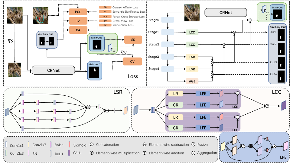
Figure 4: An overview of our proposed method. The top left figure illustrates the training process while the others show the CRNet architecture. During training, a random transform $T(\cdot)$ is applied to the input. Both the input and the transform are fed into the network, resulting in two outputs, and the CV loss is then computed based on them. $F_{ss}$ is the feature map of the input extracted from the CRNet and used to compute SS loss. The PCE, IV, CA loss are computed on auxiliary outputs and main outputs. Our contrast and relation network (CRNet) applies local-context contrasted (LCC) modules at the second and third stages, logical semantic relation (LSR) modules at the last two stages, and the auxiliary global extractor (AGE) at the last stage.

Overall Structure

The overall framework, including the proposed Contrast and Relation Network (CRNet) and loss functions, is shown in Figure 4. We first feed the input to the backbone ResNet-50 (He et al. 2016) to obtain multi-scale input features $f_{i}$, where $i\in\{x|0\leq x\leq 4,x\in\mathbb{N}\}$ denotes the stages of the backbone. CRNet uses local-context contrasted (LCC) modules for low-level features $F_{1}$, $F_{2}$ to extract contrasted features $F_{c}^{0}$, $F_{c}^{1}$, and logical semantic relation (LSR) modules for high-level input features $F_{3}$, $F_{4}$ to learn logical semantic information $F_{s}^{0}$, $F_{s}^{1}$. In addition, we design an auxiliary global extractor (AGE), a pyramid pooling module (Zhao et al. 2017) with GELU activation functions, to further acquire global semantic information $F_{s}^{g}$. Following the multiplication fusion and cross aggregation strategy (Zhao et al. 2021), we then fuse $F_{s}^{1}$ with $F_{s}^{0}$ and $F_{s}^{g}$, and integrate logical semantic information in $F_{l}^{0}$ and $F_{l}^{1}$, respectively. After aggregating $F_{c}^{0}$ with $F_{l}^{0}$ to $F_{out}^{0}$, $F_{c}^{1}$ with $F_{l}^{1}$ to $F_{out}^{1}$, CRNet further processes $F_{out}^{0}$ and $F_{out}^{1}$ and outputs multi-level segmentation maps (main output $P$ and auxiliary output $P_{1}\text{ to }P_{4}$). We also extract an intermediate feature map ($F_{ss}$) for loss computation. During training, feature-guided loss (context affinity (CA) loss and semantic significance (SS) loss) are applied to guide the segmentation, while consistency loss (cross-view (CV) and inside-view (IV) loss) ensures the consistency of predictions.

Local-Context Contrasted (LCC) Module

As camouflaged objects usually share different low-level features (e.g., texture, color, intensity) with backgrounds, it is not easy to notice the inconspicuous differences. Visual inhibition on the mammalian retina enhances the sharpness and contrast in visual response by inhibiting the activities of neighbor cells (Von Békésy 2017). Inspired by this, we propose a local-context contrasted (LCC) module to capture and strengthen low-level differences. Here, a low-level contrasted extractor (LCE) uses two low-level feature extractors (LFE) with different receptive fields to represent local and context features (i.e., neighbors), and computes the difference to increase low-level contrast and sharpness. Furthermore, We stack two LCEs in LCC to further strengthen the low-level contrasts. The contrast information learned by LCC helps expand scribbles to potential camouflaged regions, allowing our method to better command the object’s primary structure and potential boundary.

LCC processes the input low-level features $F_{in}$, which contain informative texture, color, and intensity characteristics through two branches of low-level contrasted extractors with different receptive fields. We first reduce $F_{in}$’s channel number to 64 by a 1$\times$1 convolutional layer with batch normalization and ReLU, and then take the obtained $F_{low}\in 64\times H\times W$ to two low-level contrasted extractors (LCEs) focusing on different sizes of fields. An LCE consists of a local receptor (LR), a context receptor (CR), and two low-level feature extractors (LFE). $F_{low}$ go through an LR, which is a 3$\times$3 convolutional layer with 1 dilation rate and an LFE to obtain $F_{local}$. Meanwhile, $F_{low}$ are also extracted by a CR, which is a 3$\times$3 convolutional layer with dilation $d_{context}$, and further by an LFE for $F_{context}$. We take the subtraction of $F_{local}$ and $F_{context}$ into batch normalization and ReLU to get one level contrasted features $F_{contrast}$. We set $d_{context}$ to 4 and 8 for two levels of LCE, extracting low-level contrasted features $F_{contrast}^{1}$ and $F_{contrast}^{2}$ concentrating on different sizes of receptive fields. The final output is a concatenation of $F_{contrast}^{1}$ and $F_{contrast}^{2}$. Refer to the Supplemental for LCC implementation details.

Logical Semantic Relation (LSR) Module

Scribble annotation may only annotate a part of the background. When the background consists of many low-level contrasted parts (e.g., green leaves and brown branches, yellow petals, and green stems), we need logical semantic relation information to identify the real foreground and background. Hence, we propose the LSR module to extract semantic features from 4 branches. Each branch contains a sequence of convolution layers with different kernel sizes and dilation rates, representing different receptive fields. We then integrate information from all branches to exploit comprehensive semantic information with a wider receptive field to determine the real foreground and background. Refer to the Supplemental for LSR implementation details.

Feature-guided Loss

Scribble-based methods often suffer from the lack of object information provided by the limited labeled data. Previous methods (Zhang et al. 2020b; Yu et al. 2021) exploit the information by using the pixel features of images, like colors and positions, assuming that foreground objects have visually distinctive features from backgrounds. However, in COD, such features are no longer a strong cue for boundary regions. It usually requires semantic information to decide the exact boundaries. Therefore, we design feature-guided loss based on both simple visual features (context affinity loss) and complex semantic features (semantic significance loss). As shown in Figure 5(b), semantic features extracted from the model respond actively to camouflaged boundaries and provide valuable guidance in these regions.

Context Affinity Loss. Nearby pixels with similar features tend to have the same class. Following previous methods (Obukhov et al. 2019; Yu et al. 2021), we adopt the kernel method to measure the visual feature similarity (colors and positions), which is defined as:

$$K_{vis}(i,j) =\exp(-\frac{||S(i)-S(j)||^{2}}{2\sigma_{S}^{2}}-\frac{||C(i)-C(j)||^{2}}{2\sigma_{C}^{2}}),$$ (1)

where $S(i),C(i)$ are the position $(x_{i},y_{i})$ and colors $(r_{i},g_{i},b_{i})$ of pixel $i$. $\sigma_{S},\sigma_{C}$ are hyperparameters. $D(i,j)$ calculates the probability of pixel $i,j$ having different classes ($P_{i,j}$ is the probability of positive labels for pixel $i,j$), and thus the context affinity loss $L_{ca}$ encourages visually dissimilar pixels to have different labels or vice versa:

$$D(i,j)=1-P_{i}P_{j}-(1-P_{i})(1-P_{j}),$$ (2)

$$L_{ca}=\frac{1}{M}\sum_{i}\frac{1}{K_{d}(i)}\sum_{j\in K_{d}(i)}K_{vis}(i,j)D(i,j),$$ (3)

where $K_{d}(i)$ is a neighbor $n\times n$ regions ($n$ is set to 5 in our experiments) of center pixel $i$. Through context affinity loss, the model can quickly learn from the unlabeled pixels.

Semantic Significance Loss. In COD, pixels near boundaries usually resemble each other visually, and semantic features, especially those that distinguish segmented objects (thus significant), become crucial for the exact predictions. In this case, we design the semantic significance (SS) loss that utilizes significant features to refine the predictions of boundary regions.

Here, the SS loss is computed inside small boundary regions (in practice, we divide an image to $8\times 8$ region blocks ($R_{1,...,r}$) with a step size of 4). A valid boundary region is defined as an area with at least 30% of the pixels being confidently classified as foreground or background (pixels with scribble annotation or model prediction above 0.8 is confidently classified). The design has two benefits. First, in non-boundary regions, low-level visual features suffice to provide good guidance. Second, it reduces the computation cost greatly. The semantic feature map $F_{ss}\in\mathbb{R}^{H\times W\times C}$ is extracted before the final prediction layer and its gradient is stopped (like the detach operation in Pytorch). The significance of a featured channel is determined by its covariance with confidently classified predictions:

$${Sig}_{i}=cov^{\prime}(F_{ss_{i}},P),i\in\{1,...,C\},$$ (4)

where $F_{ss_{i}}$ is the feature map of the i-th channel and $cov^{\prime}$ means covariance, computed only on confidently classified pixels. The reason behind is that the above correlations roughly show how well the features distinguish the foreground and background. Low-significance features are unwanted since they may include the “camouflaged” parts of the object and confuse the model.

We then take the top $N$ channels ordered by ${Sig}$ to form significant feature map $\hat{F_{ss}}\in\mathbb{R}^{H\times W\times N}$. In this task, we set $N$ to 16 to balance between performance and computation cost. The semantic significance loss has a similar formulation to context affinity loss:

$$K_{sem} =\exp(-\frac{||S(i)-S(j)||^{2}}{2\sigma_{S}^{2}}-\frac{||\hat{F_{ss}}(i)-\hat{F_{ss}}(j)||^{2}}{2\sigma_{C}^{2}}),$$ (5)

$$L_{ss} =w_{ss}\frac{1}{M}\sum_{k}\frac{1}{|R_{k}|}\sum_{i,j\in R_{k}}K_{sem}(i,j)D(i,j),$$ (6)

where $S(i)$ is the position of the pixel, $R_{k}$ are valid boundary regions, and $w_{ss}$ is set to increase with the epoch number (exponential ramp-up to 0.15 in practice) since the model has not learned well-represented features at the beginning.

In conclusion, the feature loss $L_{ft}$ can be written as the sum of both loss in $L_{ft}=L_{ca}+L_{ss}$.

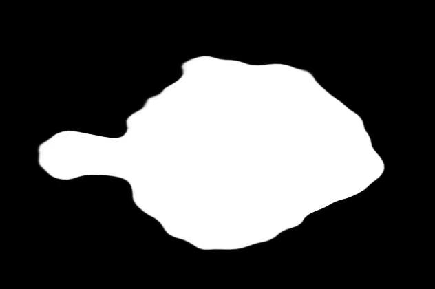
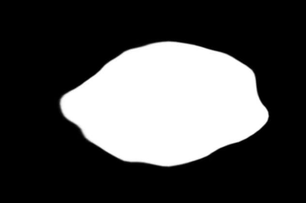
Input GT Pred. Pred.^′
(a) Predictions on input (Pred.) and its transform (Pred.^′)

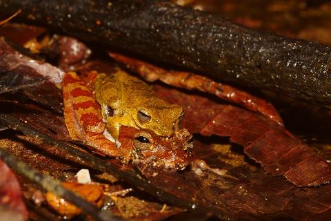
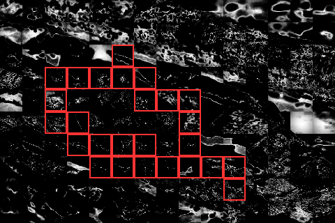
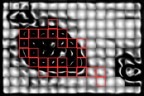
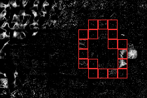
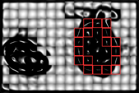
Input GT VF SS
(b) Visualization of the visual featured (VF) and semantic featured (SS) kernels

Figure 5: (a) shows that prediction on normal input is more accurate than on its transform. The design of the CV loss considers this reliability bias; (b) visualizes kernels of the visual features (VF) in $K_{vis}$ and learnt semantic features (SS) in $K_{sem}$. Images are divided into $32\times 32$ blocks (red blocks means boundary regions). We calculate the kernels with respect to the center pixels (anchors) inside blocks. White indicates high energy when the pixel label differs from the anchor.

Consistency Loss

Weakly-supervised methods often suffer from inconsistent predictions. Similar to self-consistency mechanisms in self-supervision and weakly-supervision (Laine and Aila 2016; Mittal, Tatarchenko, and Brox 2019; Yu et al. 2021; Pan et al. 2021), we propose the cross-view (CV) consistency loss to alleviate the problem by minimizing the difference between the predictions of the input and its transform. Compared to others, the CV loss excels in that it considers the reliable difference. As shown in Figure 5(a), we observe that the model has more reliable output with normal input than transformed input, which is plausible considering more loss functions are computed on normal input. The proposed CV loss pushes the predictions to the reliable one and leads to a solid improvement in performance. In addition, the predictions tend to be uncertain due to visual similarity between background and foreground in COD, and we design an inside-view consistency loss to improve the stability of predictions.

Table 1: Quantitative comparison with state-of-the-arts on three benchmarks. “F”, “U”, and “W” denote fully-supervised, unsupervised, and weakly-supervised methods, respectively.

		CAMO				CHAMELEON				COD10K
Methods	Sup.	MAE$\downarrow$	S${}_{m}\uparrow$	E${}_{m}\uparrow$	F${}_{\beta}^{w}\uparrow$	MAE$\downarrow$	S${}_{m}\uparrow$	E${}_{m}\uparrow$	F${}_{\beta}^{w}\uparrow$	MAE$\downarrow$	S${}_{m}\uparrow$	E${}_{m}\uparrow$	F${}_{\beta}^{w}\uparrow$
NLDF (Luo et al. 2017)	F	0.123	0.665	0.664	0.495	0.063	0.798	0.809	0.652	0.059	0.701	0.709	0.473
PiCANet (Liu, Han, and Yang 2018)	F	0.125	0.701	0.716	0.510	0.085	0.765	0.778	0.552	0.081	0.696	0.712	0.415
CPD (Wu, Su, and Huang 2019a)	F	0.113	0.716	0.723	0.556	0.048	0.857	0.874	0.731	0.053	0.750	0.776	0.531
EGNet (Zhao et al. 2019)	F	0.109	0.732	0.800	0.604	0.065	0.797	0.860	0.649	0.061	0.736	0.810	0.517
PoolNet (Liu et al. 2019)	F	0.105	0.730	0.746	0.575	0.054	0.845	0.863	0.690	0.056	0.740	0.776	0.506
SCRN (Wu, Su, and Huang 2019b)	F	0.090	0.779	0.797	0.643	0.042	0.876	0.889	0.741	0.047	0.789	0.817	0.575
F3Net (Wei, Wang, and Huang 2020)	F	0.109	0.711	0.741	0.564	0.047	0.848	0.894	0.744	0.051	0.739	0.795	0.544
CSNet (Gao et al. 2020)	F	0.092	0.771	0.795	0.641	0.047	0.856	0.868	0.718	0.047	0.778	0.809	0.569
ITSD (Zhou et al. 2020)	F	0.102	0.750	0.779	0.610	0.057	0.814	0.844	0.662	0.051	0.767	0.808	0.557
MINet (Pang et al. 2020)	F	0.090	0.748	0.791	0.637	0.036	0.855	0.914	0.771	0.042	0.770	0.832	0.608
PraNet (Fan et al. 2020b)	F	0.094	0.769	0.825	0.663	0.044	0.860	0.907	0.763	0.045	0.789	0.861	0.629
UCNet (Zhang et al. 2020a)	F	0.094	0.739	0.787	0.640	0.036	0.880	0.930	0.817	0.042	0.776	0.857	0.633
SINet (Fan et al. 2020a)	F	0.092	0.745	0.804	0.644	0.034	0.872	0.936	0.806	0.043	0.776	0.864	0.631
SLSR (Lv et al. 2021)	F	0.080	0.787	0.838	0.696	0.030	0.890	0.935	0.822	0.037	0.804	0.880	0.673
MGL-R (Zhai et al. 2021)	F	0.088	0.775	0.812	0.673	0.031	0.893	0.917	0.812	0.035	0.814	0.851	0.666
PFNet (Mei et al. 2021)	F	0.085	0.782	0.841	0.695	0.033	0.882	0.931	0.810	0.040	0.800	0.877	0.660
UJSC (Li et al. 2021)	F	0.073	0.800	0.859	0.728	0.030	0.891	0.945	0.833	0.035	0.809	0.884	0.684
C2FNet (Sun et al. 2021)	F	0.080	0.796	0.854	0.719	0.032	0.888	0.935	0.828	0.036	0.813	0.890	0.686
UGTR (Yang et al. 2021)	F	0.086	0.784	0.822	0.684	0.031	0.888	0.910	0.794	0.036	0.817	0.852	0.666
ZoomNet (Youwei et al. 2022)	F	0.066	0.820	0.892	0.752	0.023	0.902	0.958	0.845	0.029	0.838	0.911	0.729
DUSD (Zhang et al. 2018)	U	0.166	0.551	0.594	0.308	0.129	0.578	0.634	0.316	0.107	0.580	0.646	0.276
USPS (Nguyen et al. 2019)	U	0.207	0.568	0.641	0.399	0.188	0.573	0.631	0.380	0.196	0.519	0.536	0.265
SS (Zhang et al. 2020b)	W	0.118	0.696	0.786	0.562	0.067	0.782	0.860	0.654	0.071	0.684	0.770	0.461
SCWSSOD (Yu et al. 2021)	W	0.102	0.713	0.795	0.618	0.053	0.792	0.881	0.714	0.055	0.710	0.805	0.546
Ours	W	0.092	0.735	0.815	0.641	0.046	0.818	0.897	0.744	0.049	0.733	0.832	0.576

Cross-View Consistency Loss. For a neural network function $f_{\theta}(\cdot)$ with parameter $\theta$, some transformations $T(\cdot)$, input $x$, the ideal situation is $f_{\theta}(T(x))=T(f_{\theta}(x))$. Here, the transform includes combinations of resizing, flipping, translation and cropping, and is randomly chosen. The choice of it is explored in the ablation study. As regularization, we use the similar consistency loss $L_{cv^{\prime}}$ (Yu et al. 2021) to push them towards each other.

$$Sm(p_{1},p_{2})={1-{SSIM}(p_{1},p_{2})\over 2},$$ (7)

$$L_{cv^{\prime}}(P_{1},P_{2})={1\over M}\sum_{i}(1-\alpha)\cdot Sm(P_{1_{i}},P_{2_{i}})+\alpha|P_{1_{i}}-P_{2_{i}}|,$$ (8)

where SSIM is single scale SSIM (Godard, Mac Aodha, and Brostow 2017). $p_{1},p_{2}$ are two pixels. $\alpha$ is 0.85. $P_{1},P_{2}$ are prediction maps of the input and its transform. $M$ is the total number of pixels and $i$ is a pixel index.

Considering the above-mentioned reliability bias, we aim for the predictions of the transform $\hat{P}$ to be pushed more than that of the normal input $P$. The key here is to weight their backward gradient differently, and the proposed cross-view consistency loss can be written as:

$$L_{cv\ } =(1+\gamma)L_{cv^{\prime}}(P^{d},\hat{P})+(1-\gamma)L_{cv^{\prime}}(P,\hat{P}^{d}),$$ (9)

where $P^{d},\hat{P}^{d}$ have the same values as $P,\hat{P}$ yet the gradient on them will be ignored during back-propagation (like the detach operation in PyTorch). If $\gamma=0$, it is the original loss $L_{cv^{\prime}}$; if $\gamma>0$, the backward gradient that pushes $\hat{P}$ to $P$ is greater than the other way around, and thus the goal is reached. In practice, $\gamma$ is set to 0.3.

Inside-view Consistency Loss. We note that uncertain predictions are likely to be inconsistent. Therefore, we present the inside-view consistency (IV) loss which ”looks” inside the output and encourages predictions with high certainty by minimizing their entropy. We also use a soft indicator to filter out noisy predictions: when the entropy is above a certain threshold, the prediction result is not sure and it is malicious to increase the certainty of the model in this case. The inside-view consistency loss is as below.

$$L_{iv} =w_{iv}\cdot{1\over|I-\mathcal{B}|}\sum_{(i)\in{I-\mathcal{B}}}-P_{i}\log P_{i}-(1-P_{i})\log(1-P_{i}),$$ (10)

where $I,\mathcal{B}$ are the set of all pixels and noisy pixels. $i$ is the pixel index. $w_{iv}$ is the weight of this loss and set to 0.05 in practice. The entropy threshold for the near-boundary pixel is set to 0.5 empirically. The loss is added in the late stage of training when predictions are relatively accurate.

Combined with all the consistency losses, we have the final consistency loss: $L_{cst}=L_{cv}+L_{iv}$.

Objective Function

Below is PCE loss, where $\tilde{P}$ is the set of labeled pixels in the scribble map, $y_{i}$ is the true class of pixel $i$, and $\hat{y_{i}}$ are the predictions on pixel $i$:

$$L_{pce} ={1\over N}\sum_{i\in\tilde{P}}-y_{i}\log{\hat{y}_{i}}-(1-y_{i})\log({1-\hat{y}_{i}}),$$ (11)

We compute all losses on main output $P$ while for the auxiliary outputs ($P_{1...4}$), we compute only the PCE loss, inside-view consistency, and context affinity loss. $L_{aux}^{i}=L_{pce}^{i}+L_{ca}^{i}+L_{iv}^{i}(i=1,2,3,4)$, where $L_{aux}^{i}$ is the loss function applied to the i-th auxiliary output. Here, we do not include the other two losses for their small improvement, possibly because they require high-level feature representations or accurate segmentation to guide the model. Every output is up-sampled by linear interpolation to the same size as the input. Finally, the total objective function of our output is: $L=L_{cst}+L_{ft}+L_{pce}+\sum_{i=1}^{4}\beta_{i}L_{aux}^{i}$, where $\beta_{i}={1-0.2i}$.

Experiments

Datasets and Implementation Details

Datasets. Our experiments are conducted on three COD benchmarks, CAMO(Le et al. 2019), CHAMELEON(Skurowski et al. 2018), and COD10K(Fan et al. 2020a). Following previous studies (Fan et al. 2020a; Mei et al. 2021; Zhai et al. 2021), we relabel 4,040 images (3,040 from COD10K, 1,000 from CAMO) and propose the S-COD dataset for training. The remaining is for testing.

Evaluation Metrics. We adopt four evaluation metrics: Mean Absolute Error (MAE), S-measure $S_{m}$ (Fan et al. 2017), E-measure ($E_{m}$) (Fan et al. 2018), and weighted F-measure $F_{\beta}^{w}$ (Margolin, Zelnik-Manor, and Tal 2014).

Implementation Details. We implement our method with PyTorch and conduct experiments on a GeForce RTX2080Ti GPU. In the training phase, input images are resized to 320$\times$320 with horizontal flips. We use the stochastic gradient descent (SGD) optimizer with a momentum of 0.9, a weight decay of 5e-4, and triangle learning rate schedule with maximum learning rate 1e-3. The batch size is 16, and the training epoch is 150. It takes around 5 hours to train. As for the inference process, input images are only resized to 320$\times$320. We then directly predict the final maps without any post-processing (e.g., CRF).

Analysis

Comparison with State-of-the-arts. As we propose the first weakly-supervised method, we introduce 2 scribble-based weakly and 2 unsupervised SOD methods for comparison. We also provide the results of fully-supervised 8 COD and 12 SOD methods for reference. Quantitative comparisons are demonstrated in Table 1. Our method performs the best under four metrics on three benchmarks among weakly or unsupervised methods. It achieves an average enhancement of 11.0$\%$ on MAE, 3.2$\%$ on S-measure, 2.5$\%$ on E-measure, and 4.4$\%$ on weighted F-measure than the state-of-the-art method SCWSSOD (Yu et al. 2021). In addition, it outperforms 7 fully-supervised methods (Luo et al. 2017; Liu, Han, and Yang 2018; Wu, Su, and Huang 2019a; Zhao et al. 2019; Liu et al. 2019; Wei, Wang, and Huang 2020; Zhou et al. 2020). We also find that our method has the largest improvement in CAMO (outperforms nearly all fully-supervised SOD methods and is close to COD methods), which is the most challenging one among all of the 3 COD datasets (worst metric value). This shows that our method is indeed better at discovering hard camouflage objects than others. Figure 6 shows that our method performs well in various challenging scenarios, including high intrinsic similarities (row 1), tiny objects (row 2), complex backgrounds (row 3), and multiple objects (row 4).

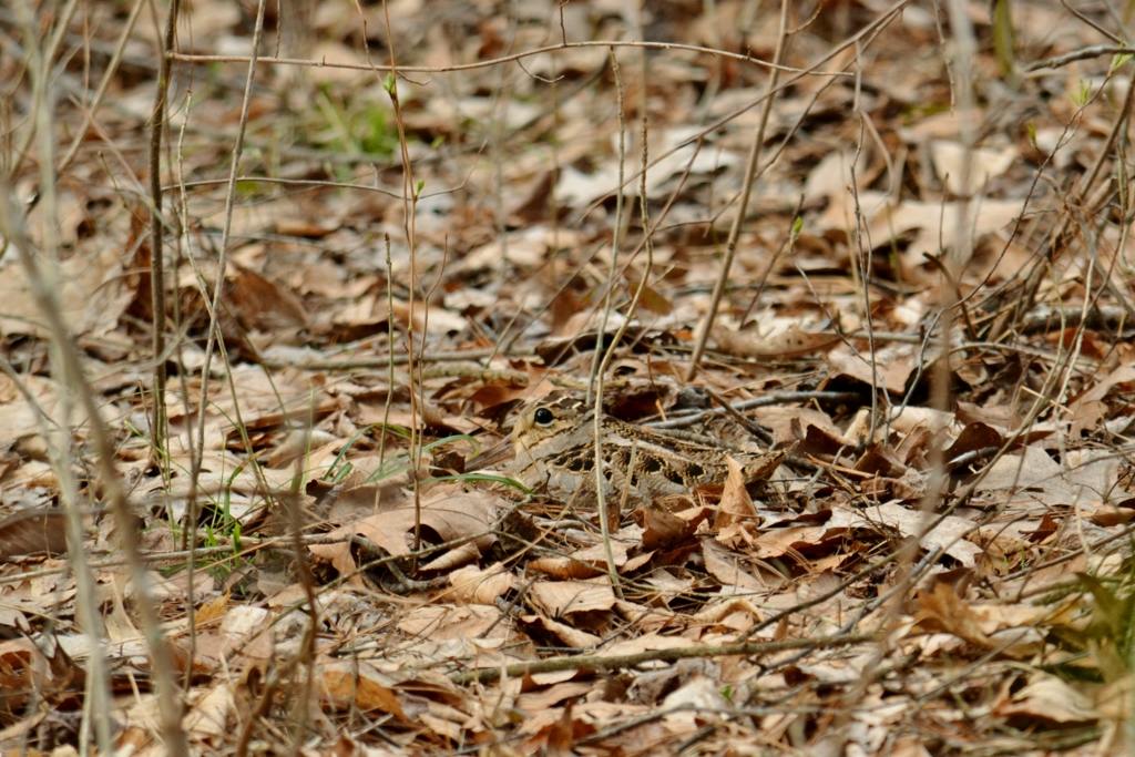
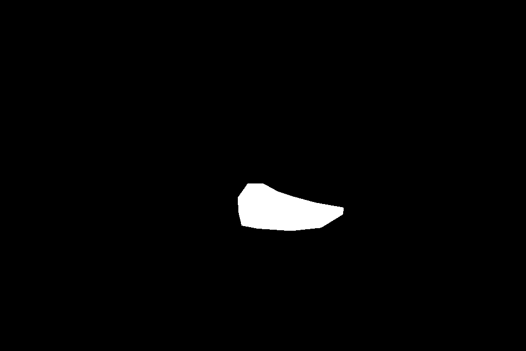
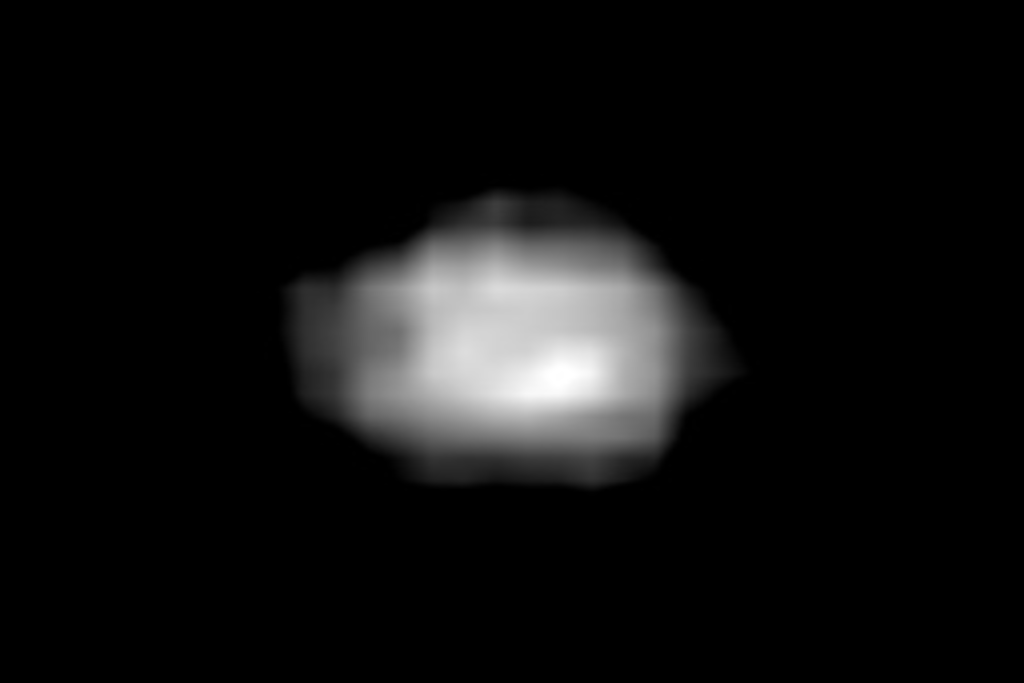
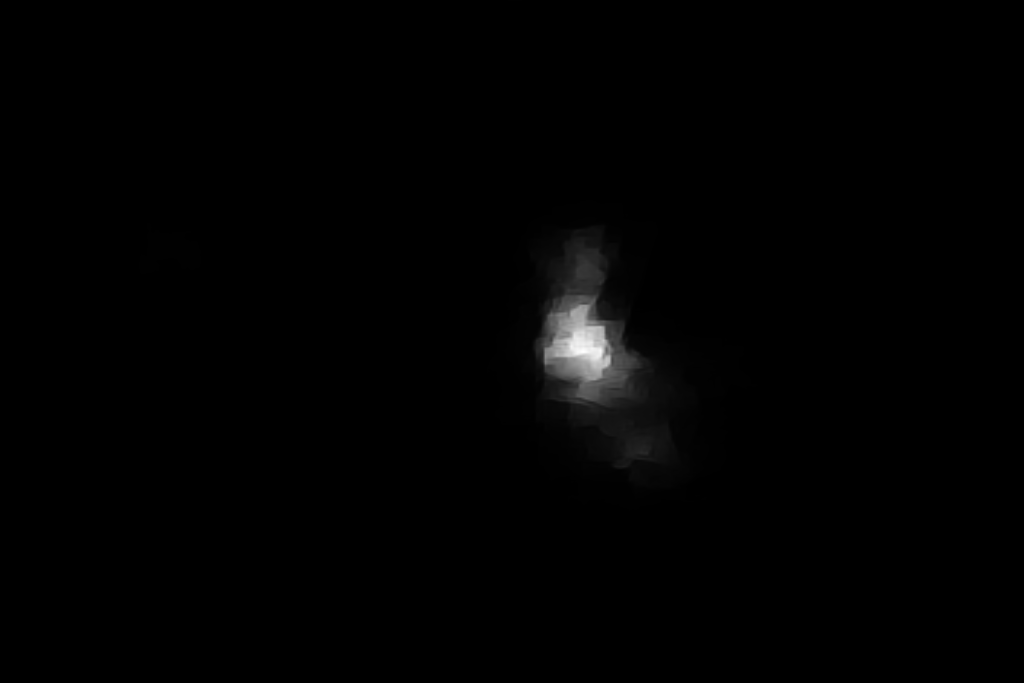
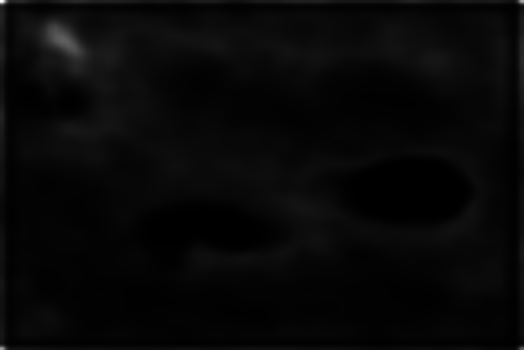
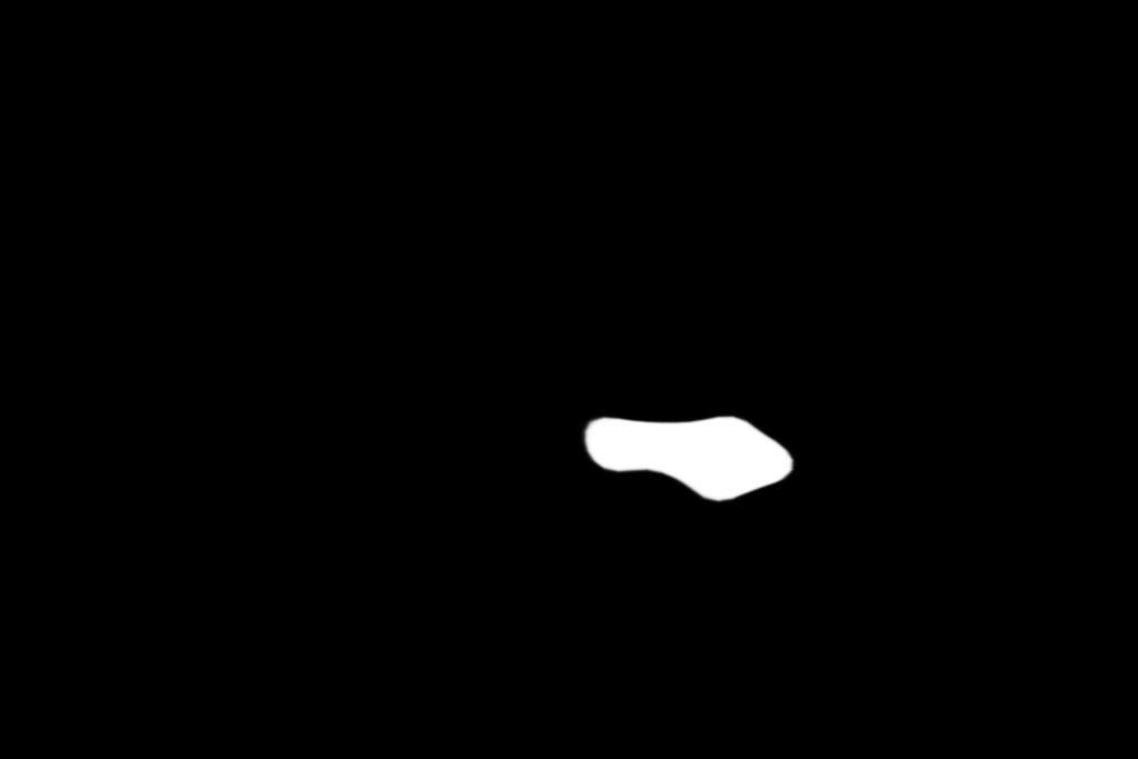
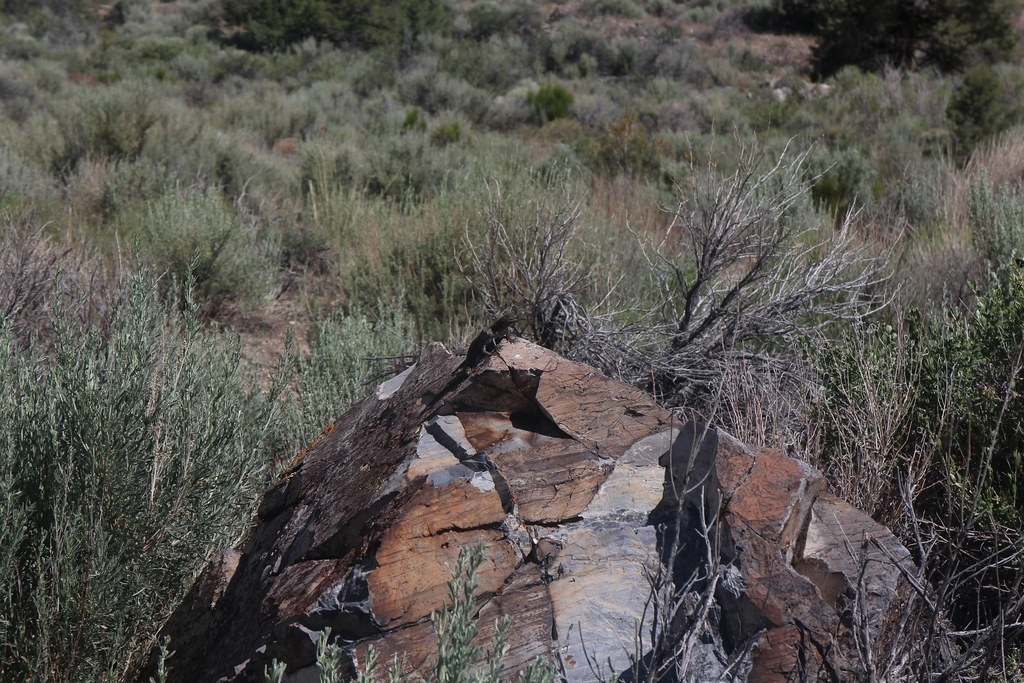
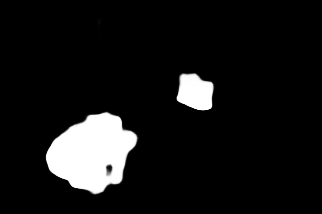
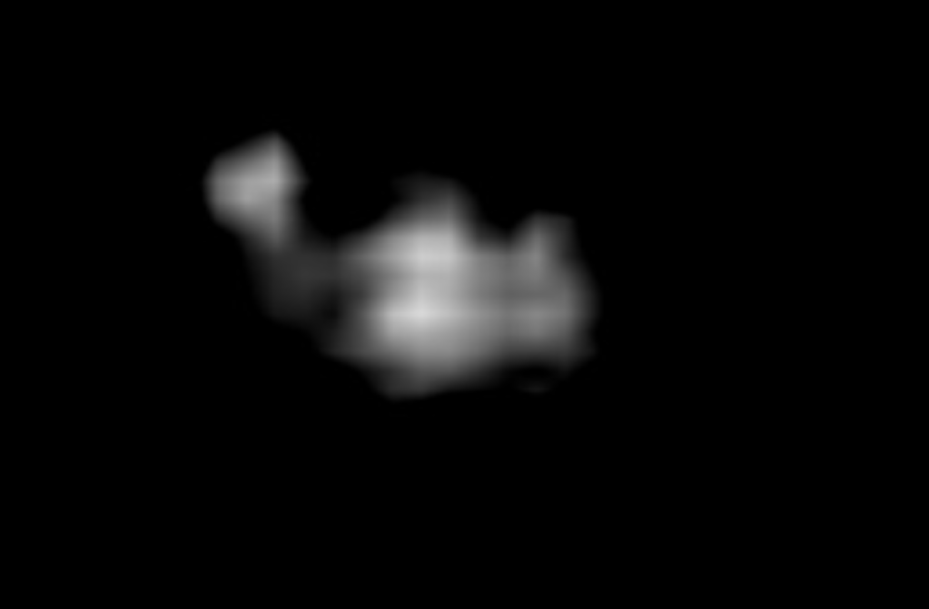
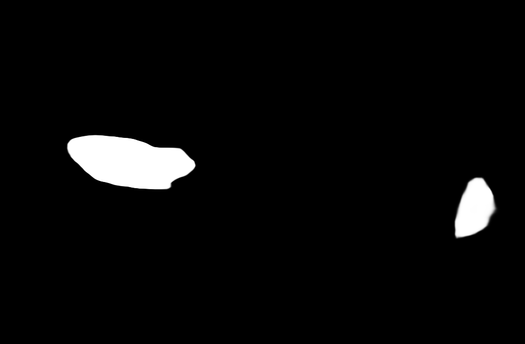
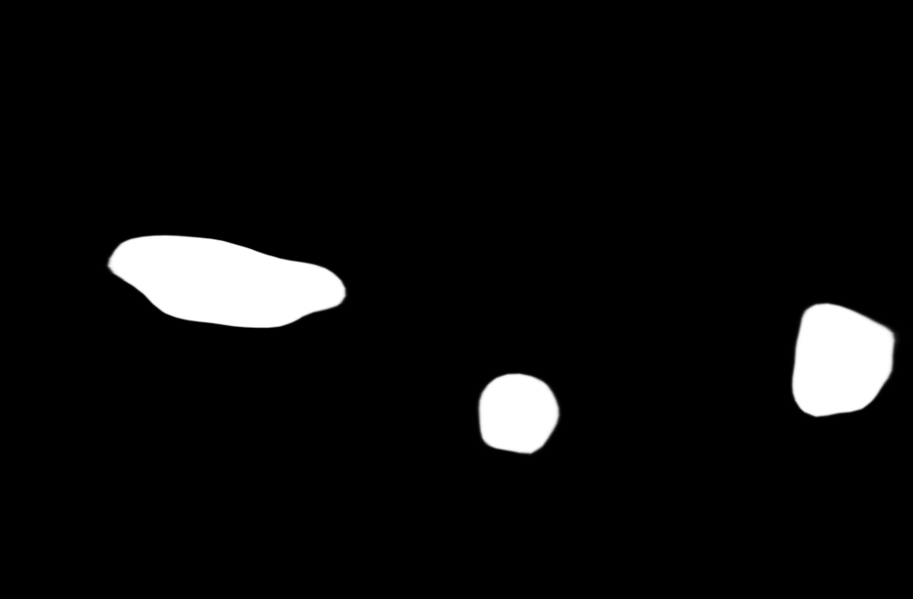
Input GT ZoomNet UGTR DUSD SS SCWSSOD Ours

Figure 6: Qualitative comparison of our method with state-of-the-arts fully-supervised, unsupervised, and scribble-based weakly-supervised methods in challenging scenarios.

Ablation Studies on Modules. To verify the effectiveness of our modules, we conduct ablation studies on challenging dataset CAMO (Le et al. 2019), where the methods obtain the worst scores according to Table 1. Table LABEL:tab:componentAblation shows only using a backbone (BB) performs worst (i.e., Ablation I), while adding LCC or LSR improves performances on different metrics. As shown in Figure 7, LCC finds potential camouflaged regions with low-level contrasts, but it may be confused by complex background (e.g., many distinct leaves). Meanwhile, LSR analyzes logical semantic relations between different parts, but it may segment inaccurate boundaries. When LCC and LSR cooperate to detect camouflaged objects (Ours), the performance is enhanced dramatically from the single module usage (III, IV). It shows the effectiveness of CRNet design.

Table 2: The ablation study results of components on CAMO (Le et al. 2019).

Methods	BB	AGE	LCC	LSR	MAE$\downarrow$	S${}_{m}\uparrow$	E${}_{m}\uparrow$	F${}_{\beta}^{w}\uparrow$
Ablation I	$\surd$				0.104	0.701	0.774	0.598
Ablation II	$\surd$	$\surd$			0.100	0.716	0.799	0.615
Ablation III	$\surd$	$\surd$	$\surd$		0.099	0.721	0.806	0.626
Ablation IV	$\surd$	$\surd$		$\surd$	0.098	0.713	0.783	0.612
Ours	$\surd$	$\surd$	$\surd$	$\surd$	0.092	0.735	0.815	0.641

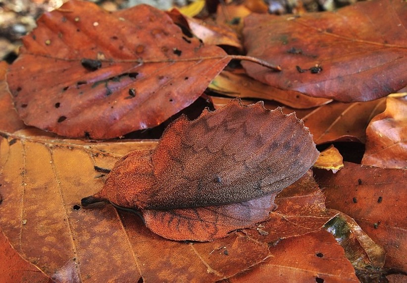
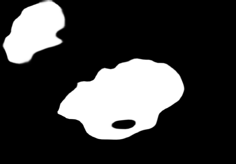
Input GT I II III IV Ours

Figure 7: A visual example of the component ablation study.

Ablation Studies on Loss Functions. A detailed ablation study for loss functions is also conducted in Table LABEL:tab:lossAblation. We first explore various combinations of transformation operations in cross-view consistency. It is shown that flipping, translating, and cropping upgrade the performance significantly. The second group, the ablation of consistency loss, shows improvements on all metrics except MAE. This indicates the benefit of the proposed consistency mechanism. The third group ablates our feature-guided loss. The final group is the overall component ablation of consistency loss and feature-guided loss. We see that both losses provide tremendous improvement in the test dataset.

Table 3: The ablation study for our loss functions on CAMO (Le et al. 2019). Groups correspond to ablations on transformations in cross-view consistency, on consistency loss, on feature loss, and on all losses. Here, pce stands for partial cross-entropy; ft and cs stand for feature-guided loss and consistency loss (cs=cv+iv, ft=ca+ss); cv and iv stand for cross-view and inside-view consistency loss; cv’ means cross-view consistency without reliability bias; cv($\cdot$) specifies the transforms used in computing cv; R,F,T,C are resizing, flipping, translation and cropping .

Basic setting	Loss	MAE$\downarrow$	S${}_{m}\uparrow$	E${}_{m}\uparrow$	F${}_{\beta}^{w}\uparrow$
w/ pce	Baseline	0.215	0.612	0.633	0.387
w/ ft, iv	w/o cv	0.105	0.721	0.786	0.600
	w/ cv(R)	0.097	0.727	0.807	0.629
	w/ cv(R, F)	0.094	0.730	0.812	0.638
	w/ cv(R, F, T)	0.094	0.730	0.808	0.637
	w/ cv(R, F, T, C)	0.092	0.735	0.815	0.641
w/ ft	w/ cv’	0.095	0.723	0.801	0.624
	w/ cv	0.095	0.726	0.804	0.632
	w/ cs	0.092	0.735	0.815	0.641
w/ cs	w/ ca	0.095	0.727	0.807	0.631
	w/ ft	0.092	0.735	0.815	0.641
w/ pce	w/ cs	0.096	0.731	0.821	0.641
	w/ ft	0.107	0.720	0.785	0.592
	w/ cs, ft	0.092	0.735	0.815	0.641

Conclusion

In this paper, we propose the first weakly-supervised COD dataset with scribble annotation, which takes ~10 seconds to label an image (360 times faster than pixel-wise annotation). To overcome the weaknesses of current weakly-supervised learning and their application to COD, we propose a novel framework consisting of two loss functions and a novel network: a consistency loss, including consistency inside and cross images, regulates the model to have coherent predictions, and incline them to more reliable ones; a feature-guided loss locates the ”hidden” foreground by comparing both manually computed visual features and learned semantic features of each pixel. The proposed network learns low-level contrast to expand scribbles to wider potential regions first and then analyzes logical semantic relation information to determine the real foreground and background. Experimental results show our method outperforms unsupervised and weakly-supervised state-of-the-arts with improvement, and is even competitive with the fully-supervised methods.

References

- Fan et al. (2017) Fan, D.-P.; Cheng, M.-M.; Liu, Y.; Li, T.; and Borji, A. 2017. Structure-measure: A new way to evaluate foreground maps. In Proceedings of the IEEE international conference on computer vision, 4548–4557.
- Fan et al. (2018) Fan, D.-P.; Gong, C.; Cao, Y.; Ren, B.; Cheng, M.-M.; and Borji, A. 2018. Enhanced-alignment measure for binary foreground map evaluation. arXiv preprint arXiv:1805.10421.
- Fan et al. (2021) Fan, D.-P.; Ji, G.-P.; Cheng, M.-M.; and Shao, L. 2021. Concealed object detection. IEEE Transactions on Pattern Analysis and Machine Intelligence.
- Fan et al. (2020a) Fan, D.-P.; Ji, G.-P.; Sun, G.; Cheng, M.-M.; Shen, J.; and Shao, L. 2020a. Camouflaged object detection. In Proceedings of the IEEE/CVF conference on computer vision and pattern recognition, 2777–2787.
- Fan et al. (2020b) Fan, D.-P.; Ji, G.-P.; Zhou, T.; Chen, G.; Fu, H.; Shen, J.; and Shao, L. 2020b. Pranet: Parallel reverse attention network for polyp segmentation. In International conference on medical image computing and computer-assisted intervention, 263–273. Springer.
- Fan et al. (2020c) Fan, D.-P.; Zhou, T.; Ji, G.-P.; Zhou, Y.; Chen, G.; Fu, H.; Shen, J.; and Shao, L. 2020c. Inf-net: Automatic covid-19 lung infection segmentation from ct images. IEEE Transactions on Medical Imaging, 39(8): 2626–2637.
- Gao et al. (2020) Gao, S.-H.; Tan, Y.-Q.; Cheng, M.-M.; Lu, C.; Chen, Y.; and Yan, S. 2020. Highly efficient salient object detection with 100k parameters. In European Conference on Computer Vision, 702–721. Springer.
- Godard, Mac Aodha, and Brostow (2017) Godard, C.; Mac Aodha, O.; and Brostow, G. J. 2017. Unsupervised monocular depth estimation with left-right consistency. In Proceedings of the IEEE conference on computer vision and pattern recognition, 270–279.
- He et al. (2016) He, K.; Zhang, X.; Ren, S.; and Sun, J. 2016. Deep residual learning for image recognition. In Proceedings of the IEEE conference on computer vision and pattern recognition, 770–778.
- Hubel and Wiesel (1962) Hubel, D. H.; and Wiesel, T. N. 1962. Receptive fields, binocular interaction and functional architecture in the cat’s visual cortex. The Journal of physiology, 160(1): 106.
- Laine and Aila (2016) Laine, S.; and Aila, T. 2016. Temporal ensembling for semi-supervised learning. arXiv preprint arXiv:1610.02242.
- Le et al. (2019) Le, T.-N.; Nguyen, T. V.; Nie, Z.; Tran, M.-T.; and Sugimoto, A. 2019. Anabranch network for camouflaged object segmentation. Computer Vision and Image Understanding, 184: 45–56.
- Li et al. (2021) Li, A.; Zhang, J.; Lv, Y.; Liu, B.; Zhang, T.; and Dai, Y. 2021. Uncertainty-aware joint salient object and camouflaged object detection. In Proceedings of the IEEE/CVF Conference on Computer Vision and Pattern Recognition, 10071–10081.
- Lin et al. (2022) Lin, J.; Tan, X.; Xu, K.; Ma, L.; and Lau, R. W. 2022. Frequency-aware Camouflaged Object Detection. ACM Transactions on Multimedia Computing, Communications, and Applications (TOMM).
- Liu et al. (2019) Liu, J.-J.; Hou, Q.; Cheng, M.-M.; Feng, J.; and Jiang, J. 2019. A simple pooling-based design for real-time salient object detection. In Proceedings of the IEEE/CVF conference on computer vision and pattern recognition, 3917–3926.
- Liu, Han, and Yang (2018) Liu, N.; Han, J.; and Yang, M.-H. 2018. Picanet: Learning pixel-wise contextual attention for saliency detection. In Proceedings of the IEEE conference on computer vision and pattern recognition, 3089–3098.
- Luo et al. (2017) Luo, Z.; Mishra, A.; Achkar, A.; Eichel, J.; Li, S.; and Jodoin, P.-M. 2017. Non-local deep features for salient object detection. In Proceedings of the IEEE Conference on computer vision and pattern recognition, 6609–6617.
- Lv et al. (2021) Lv, Y.; Zhang, J.; Dai, Y.; Li, A.; Liu, B.; Barnes, N.; and Fan, D.-P. 2021. Simultaneously localize, segment and rank the camouflaged objects. In Proceedings of the IEEE/CVF Conference on Computer Vision and Pattern Recognition, 11591–11601.
- Margolin, Zelnik-Manor, and Tal (2014) Margolin, R.; Zelnik-Manor, L.; and Tal, A. 2014. How to evaluate foreground maps? In Proceedings of the IEEE conference on computer vision and pattern recognition, 248–255.
- Mei et al. (2021) Mei, H.; Ji, G.-P.; Wei, Z.; Yang, X.; Wei, X.; and Fan, D.-P. 2021. Camouflaged object segmentation with distraction mining. In Proceedings of the IEEE/CVF Conference on Computer Vision and Pattern Recognition, 8772–8781.
- Mittal, Tatarchenko, and Brox (2019) Mittal, S.; Tatarchenko, M.; and Brox, T. 2019. Semi-supervised semantic segmentation with high-and low-level consistency. IEEE transactions on pattern analysis and machine intelligence, 43(4): 1369–1379.
- Nguyen et al. (2019) Nguyen, T.; Dax, M.; Mummadi, C. K.; Ngo, N.; Nguyen, T. H. P.; Lou, Z.; and Brox, T. 2019. Deepusps: Deep robust unsupervised saliency prediction via self-supervision. Advances in Neural Information Processing Systems, 32.
- Obukhov et al. (2019) Obukhov, A.; Georgoulis, S.; Dai, D.; and Van Gool, L. 2019. Gated CRF loss for weakly supervised semantic image segmentation. arXiv preprint arXiv:1906.04651.
- Pan et al. (2021) Pan, Z.; Jiang, P.; Wang, Y.; Tu, C.; and Cohn, A. G. 2021. Scribble-Supervised Semantic Segmentation by Uncertainty Reduction on Neural Representation and Self-Supervision on Neural Eigenspace. In Proceedings of the IEEE/CVF International Conference on Computer Vision, 7416–7425.
- Pang et al. (2020) Pang, Y.; Zhao, X.; Zhang, L.; and Lu, H. 2020. Multi-scale interactive network for salient object detection. In Proceedings of the IEEE/CVF conference on computer vision and pattern recognition, 9413–9422.
- Pérez-de la Fuente et al. (2012) Pérez-de la Fuente, R.; Delclòs, X.; Peñalver, E.; Speranza, M.; Wierzchos, J.; Ascaso, C.; and Engel, M. S. 2012. Early evolution and ecology of camouflage in insects. Proceedings of the National Academy of Sciences, 109(52): 21414–21419.
- Skurowski et al. (2018) Skurowski, P.; Abdulameer, H.; Błaszczyk, J.; Depta, T.; Kornacki, A.; and Kozieł, P. 2018. Animal camouflage analysis: Chameleon database. Unpublished manuscript, 2(6): 7.
- Sun et al. (2021) Sun, Y.; Chen, G.; Zhou, T.; Zhang, Y.; and Liu, N. 2021. Context-aware Cross-level Fusion Network for Camouflaged Object Detection. arXiv preprint arXiv:2105.12555.
- Von Békésy (2017) Von Békésy, G. 2017. Sensory inhibition. In Sensory Inhibition. Princeton University Press.
- Wald (1935) Wald, G. 1935. Carotenoids and the visual cycle. The Journal of general physiology, 19(2): 351–371.
- Wei, Wang, and Huang (2020) Wei, J.; Wang, S.; and Huang, Q. 2020. F3Net: fusion, feedback and focus for salient object detection. In Proceedings of the AAAI Conference on Artificial Intelligence, volume 34, 12321–12328.
- Wu, Su, and Huang (2019a) Wu, Z.; Su, L.; and Huang, Q. 2019a. Cascaded partial decoder for fast and accurate salient object detection. In Proceedings of the IEEE/CVF conference on computer vision and pattern recognition, 3907–3916.
- Wu, Su, and Huang (2019b) Wu, Z.; Su, L.; and Huang, Q. 2019b. Stacked cross refinement network for edge-aware salient object detection. In Proceedings of the IEEE/CVF international conference on computer vision, 7264–7273.
- Yang et al. (2021) Yang, F.; Zhai, Q.; Li, X.; Huang, R.; Luo, A.; Cheng, H.; and Fan, D.-P. 2021. Uncertainty-guided transformer reasoning for camouflaged object detection. In Proceedings of the IEEE/CVF International Conference on Computer Vision, 4146–4155.
- Youwei et al. (2022) Youwei, P.; Xiaoqi, Z.; Tian-Zhu, X.; Lihe, Z.; and Huchuan, L. 2022. Zoom In and Out: A Mixed-scale Triplet Network for Camouflaged Object Detection. arXiv preprint arXiv:2203.02688.
- Yu et al. (2021) Yu, S.; Zhang, B.; Xiao, J.; and Lim, E. G. 2021. Structure-consistent weakly supervised salient object detection with local saliency coherence. In Proceedings of the AAAI Conference on Artificial Intelligence (AAAI). AAAI Palo Alto, CA, USA.
- Zhai et al. (2021) Zhai, Q.; Li, X.; Yang, F.; Chen, C.; Cheng, H.; and Fan, D.-P. 2021. Mutual graph learning for camouflaged object detection. In Proceedings of the IEEE/CVF Conference on Computer Vision and Pattern Recognition, 12997–13007.
- Zhang et al. (2020a) Zhang, J.; Fan, D.-P.; Dai, Y.; Anwar, S.; Saleh, F. S.; Zhang, T.; and Barnes, N. 2020a. UC-Net: Uncertainty inspired RGB-D saliency detection via conditional variational autoencoders. In Proceedings of the IEEE/CVF conference on computer vision and pattern recognition, 8582–8591.
- Zhang et al. (2020b) Zhang, J.; Yu, X.; Li, A.; Song, P.; Liu, B.; and Dai, Y. 2020b. Weakly-supervised salient object detection via scribble annotations. In Proceedings of the IEEE/CVF conference on computer vision and pattern recognition, 12546–12555.
- Zhang et al. (2018) Zhang, J.; Zhang, T.; Dai, Y.; Harandi, M.; and Hartley, R. 2018. Deep unsupervised saliency detection: A multiple noisy labeling perspective. In Proceedings of the IEEE conference on computer vision and pattern recognition, 9029–9038.
- Zhao et al. (2017) Zhao, H.; Shi, J.; Qi, X.; Wang, X.; and Jia, J. 2017. Pyramid scene parsing network. In Proceedings of the IEEE conference on computer vision and pattern recognition, 2881–2890.
- Zhao et al. (2019) Zhao, J.-X.; Liu, J.-J.; Fan, D.-P.; Cao, Y.; Yang, J.; and Cheng, M.-M. 2019. EGNet: Edge guidance network for salient object detection. In Proceedings of the IEEE/CVF international conference on computer vision, 8779–8788.
- Zhao et al. (2021) Zhao, Z.; Xia, C.; Xie, C.; and Li, J. 2021. Complementary Trilateral Decoder for Fast and Accurate Salient Object Detection. In Proceedings of the 29th ACM International Conference on Multimedia, 4967–4975.
- Zhou et al. (2020) Zhou, H.; Xie, X.; Lai, J.-H.; Chen, Z.; and Yang, L. 2020. Interactive two-stream decoder for accurate and fast saliency detection. In Proceedings of the IEEE/CVF Conference on Computer Vision and Pattern Recognition, 9141–9150.