document

Quantifying the lucky droplet model for rainfall

Abstract

It is difficult to explain rainfall from ice-free clouds, because the timescale for the onset of rain showers is shorter than the mean time for collisions between microscopic water droplets. It has been suggested that raindrops are produced from very rare ‘lucky’ droplets, which undergo a large number of collisions on a timescale which is short compared to the mean time for a the first collision. This work uses large deviation theory to develop estimates for the timescale for the onset of a rain shower, as a function of the collision rate coefficients.

The growth history of the fast-growing droplets which do become raindrops is discussed. It is shown that their first few collisions are always approximately equally spaced in time, regardless of how the mean time for typical droplets varies as a function of the number of collisions.

1 Introduction

There are some fundamental challenges in understanding rainfall from clouds Mas71 ; Pru+97 . When ice is present, the Bergeron mechanism Mas71 shows how condensation of water vapour onto ice crystals can trigger precipitation, but when no ice is present rainfall relies on collision and coalescence of microscopic water droplets. It has proven to be difficult to understand how the rate of these collisions can be sufficient to explain rainfall Sha03 .

The collisions occur mainly as a result of microscopic water droplets with different radius falling at different terminal velocities. An important aspect of the growth of raindrops is that, because larger droplets fall more rapidly and have a larger cross-section, the collisions happen more frequently as the droplet grows. If $\tau_{n}$ is the mean time between the first $n-1$ and the first $n$ collisions, it is expected that $\tau_{n}$ decreases rapidly as a function of $n$. According to a model which is discussed in detail below, the sum

$$\langle T\rangle=\sum_{n=1}^{\cal N}\tau_{n}$$ (1)

which is the mean time for ${\cal N}$ collisions, approaches a finite limit as ${\cal N}\to\infty$. The typical radius of the microscopic droplets in clouds (which form on condensation nuclei such as salt particles from evaporated sea spray) is approximately $10\,\mu{\rm m}$, and the liquid water content of a dense cloud is approximately $1\,{\rm gm}^{-3}$ Mas71 ; Pru+97 . Using these data, the rate of collision of droplets is found to be very small. The mean time for the first collision, $\tau_{1}$, depends upon the dispersion of the droplet sizes, but it is much less than one collision per hour. A raindrop may may have a radius as large as $1\,{\rm mm}$. Because most collisions of the growing droplet are with microscopic droplets, approximately $10^{6}$ collisions are required to create a raindrop. It is common experience that newly formed clouds can generate rain showers quite rapidly, on a timescale of less than half an hour. Given the slow rate of the first few collisions, and the very large number of collisions that are required, it hard to understand how rainfall can happen so quickly.

The Lifshitz-Slyozov analysis of Ostwald ripening Lif+61 ; Lif+81 does not offer a resolution of this problem because it acts too slowly Cle08 ; Wil14 . It has also been pointed out that turbulence in cumulus clouds will enhance the collision rate Saf+56 , but extensive studies, reviewed in Pum+16 , indicate that this effect is not sufficient, except possibly in the most unstable atmospheric conditions. The most satisfying solution to this problem is the ‘lucky droplet’ concept, originally proposed by Telford Tel55 and Twomey Two66 . These authors pointed out that it is those microscopic droplets which undergo their first few collisions exceptionally quickly will grow into raindrops, and absorb a large number of other microscopic droplets in the process. In fact, the fastest growing droplets could absorb all the remaining microscopic water droplets on their way to becoming raindrops, so that the occurrence of a rain shower is determined by the growth history of the (approximately) one-in-a-million fastest growing droplets.

Subsequently, Kostinski and Shaw Kos+05 formulated a model for the time taken for droplets to grow by collision, and presented some simulations indicating that it could yield a satisfactory solution of the problem. It is desirable to have a simple and maximally transparent expression for this ‘lucky droplet’ principle. In Wil16 , it was proposed that large deviation theory Fre+84 ; Tou09 is the relevant tool. When $T$ is small, the probability $P(T)$ that a microscopic droplet undergoes runaway growth to become a rain droplet within time $T$ is exponentially small: write

$$P(T)=\exp[-{\cal J}(T)]$$ (2)

where ${\cal J}(T)$ is closely related to the entropy function or rate function in large deviation theory. If a rain droplet is the result of coalescence of ${\cal N}$ microscopic droplets, then the fraction of the microscopic droplets which are removed after time $T$ is greater than ${\cal N}P(T)$, provided the number of microscopic droplets has not yet been significantly reduced by collisions. The onset of the rain shower is at a time $T^{\ast}$ when a significant fraction of the microscopic water droplets have been removed by coalescence into falling rain drops. It will be argued that this time $T^{\ast}$ is estimated by writing ${\cal N}\exp[-{\cal J}(T^{\ast})]\sim 1$. The time $T^{\ast}$ at which a rain shower occurs is therefore estimated by solving the equation

$${\cal J}(T^{\ast})=\ln\,{\cal N}\ .$$ (3)

The function ${\cal J}(t)$ diverges as $t\to 0$. It is, therefore, expected that, in the limit as ${\cal N}\to\infty$, the ratios $T^{\ast}/\langle T\rangle$ and $T^{\ast}/\tau_{1}$ become small. This implies that, if ${\cal N}$ is sufficiently large, a rain shower is expected to occur after a time which is small compared to the mean time for the first collision.

Equation (3) offers a surprisingly simple criterion for the onset of rain showers. If the brief arguments presented above are considered more carefully, as is done in section 2 below, it can be argued that solving a variant of equation (3) gives an upper bound on the time taken to produce a rain shower, in the context of a model for a homogeneous atmosphere.

In order to make practical use of equation (3), ${\cal J}(T)$ should be expressed as a functional of the set of mean collision times $\tau_{n}$. This is addressed in section 3. Both of the earlier works which quantify the lucky droplet model, Kos+05 and Wil16 , assumed that $\tau_{n}$ has a power-law dependence upon $n$, writing $\tau_{n}=\tau_{1}n^{-\gamma}$, but it is desirable to determine ${\cal J}(T)$ in a more general case. Because the terminal velocity of a small sphere is proportional to the square of its radius $a$, and the collision cross section also increases as $a^{2}$, the collision rate is proportional to $a^{4}$ for droplets which have undergone a large number of collisions, but which have a terminal velocity with small Reynolds number. The volume of a droplet is proportional to the number of collisions that it has undergone, implying that $a^{3}\sim n$, so that the exponent is $\gamma=4/3$. However, this choice might not give a good description of the time between the first few collisions ($\tilde{n}$, say), which may occur at a different rate Mas71 ; Pru+97 (for example, collisions of very small droplets may be suppressed by lubrication effects). Accordingly, the following calculations emphasise the more general case where

$$\tau_{n}=\tau_{1}n^{-\gamma}\left[1+Q(n/\tilde{n})\right]$$ (4)

where $Q(x)$ is a positive function which approaches zero when $x\gg 1$, and which may be divergent as $x\to 0$. The objective is to give useful approximations to ${\cal J}(T)$ which are applicable in this more general case. The numerical illustrations will use

$$Q(x)=x^{-\delta}\exp(-x)$$ (5)

with $\gamma=4/3$ and $\delta>0$ (which implies that the first few collisions occur more slowly than predicted by the $\tau_{n}\sim n^{-4/3}$ relation). It will be shown that the time taken to initiate a rain shower is surprisingly insensitive to the first few values of the mean collision times $\tau_{n}$.

It is interesting to consider the growth history of the fastest growing droplets. This is addressed in section 4. Surprisingly, it is found that their first few collisions occur at approximately equally spaced time intervals, regardless of the form of dependence of $\tau_{n}$ upon $n$. To avoid unhelpful complication of the notation, section 3 considers the growth history of droplets where the collision times are a simple power-law, $\tau_{n}=n^{-\gamma}$, rather than the more general case described by (4).

The formulae developed in sections 3 and 4 are compared with numerical simulations. Section 5 is a concluding summary.

2 Modelling rain showers

Assume that there is, initially, a uniform density of microscopic water droplets in a homogeneous atmosphere. These undergo collisions, such that the density of droplets $\rho(m,t)\delta m$ in a small interval of mass, $[m,m+\delta m]$, varies as a function of time. Collision of a droplet of mass in the small interval $[m_{1},m_{1}+\delta m_{1}]$ with another droplet having mass in the small interval $[m_{2},m_{2}+\delta m_{2}]$ occurs with rate $K(m_{1},m_{2})\rho(m_{1},t)\rho(m_{2},t)\delta m_{1}\delta m_{2}$, where $K(m_{1},m_{2})$ is termed the collision kernel. The density of droplets $\rho(m,t)$ with mass $m$ after time $t$ is then specified by the Smoluchowski equation Smo16 ; Mas71 ; Pru+97 ; Sha03 ; Ald99 :

$$\frac{\partial\rho(m,t)}{\partial t} = \frac{1}{2}\int_{0}^{m}{\rm d}m^{\prime}\ K(m-m^{\prime},m^{\prime})\rho(m-m^{\prime},t)\rho(m^{\prime},t)$$ (6)

$$-\int_{0}^{\infty}{\rm d}m^{\prime}\ K(m,m^{\prime})\rho(m,t)\rho(m^{\prime},t)\ .$$

The collision kernel for small droplets falling under gravity has the form

$$K(m_{1},m_{2})=A\varepsilon(m_{1},m_{2})(m_{1}^{1/3}+m_{2}^{1/3})^{2}|m_{1}^{2/3}-m_{2}^{2/3}|$$ (7)

where $A$ is a constant and $\varepsilon(m_{1},m_{2})=\varepsilon(m_{2},m_{1})$ is a collision efficiency, which is assumed to approach unity after the first few collisions, but which may be small in the initial stages of droplet growth Mas71 ; Pru+97 ; Sha03 .

If the dispersion of the initial masses is small, the size of a droplet can be described by the number $n$ of droplets from which it has been formed by coalescence. It is this simplified picture which will be used in the following discussions, in which the initial un-collided droplets will be referred to as monomers, and the larger droplets as $n$-mers. The density of $n$-mers, $\tilde{\rho}(n,t)$, obeys a simplified Smoluchowski equation

$$\frac{\partial\tilde{\rho}(n,t)}{\partial t} = \frac{1}{2}\sum_{m=1}^{n-1}\tilde{K}(n-m,m)\tilde{\rho}(n-m,t)\tilde{\rho}(m,t)$$ (8)

$$-\sum_{m=1}^{\infty}\tilde{K}(n,m)\tilde{\rho}(n,t)\tilde{\rho}(m,t)\ .$$

Because the collision kernel, equation (7), increases sufficiently rapidly as a function of the masses, the mean time to reach an infinite cluster size is finite: in the literature of the Smoluchowski equation, this runaway growth is termed a gelation transition Ald99 . If the clusters are allowed to grow to infinite size, the Smoluchowski equation predicts that the gelation transition for the kernel (7) occurs in zero time vDo87 ; Ald99 ; Ley03 ; Bal+11 . This is a consequence of the fact that the Smoluchowski equation is a mean-field approximation: in an infinite volume, there is one cluster that grows arbitrarily quickly, and this will absorb all of the other particles.

In the application to modelling clouds, it will be assumed that the droplets grow to a finite size, achieved after ${\cal N}\approx 10^{6}$ microscopic droplets have coalesced. The size limit could be a consequence of the finite depth of the cloud, or because raindrops fragment due to aerodynamic forces above a certain size.

If this upper cutoff is imposed, it is possible in principle solve the Smoluchowski equation to calculate the probability $P(T)$ that a given droplet has grown by coalescence to size ${\cal N}$ after time $T$. Because the raindrop has absorbed ${\cal N}$ microscopic droplets in this process, if ${\cal N}P(T)=\mu$, with $0<\mu<1$, then at time $T$ a fraction of the liquid water content of the cloud greater than or equal to $\mu$ has become macroscopic rain droplets. It is, therefore, possible to estimate the time $T^{\ast}$ for the onset of a rain shower by solving the equation $P(T^{\ast})=\mu/{\cal N}$. Under typical circumstances a rain shower converts a few percent of the liquid water content into rain, so taking $\mu>0.1$ (say) would give a reasonable upper bound on the time taken to produce a rain shower.

In the context of this approach to estimating $T^{\ast}$, the fact that the Smoluchowski equation is a mean-field equation is not a deficiency, because the period between collisions is sufficiently large that the system is ‘well-mixed’. However, it is extremely difficult to determine useful analytical expressions for solutions of the Smoluchowski equation, and even if these were available, it would be difficult to use them to determine $P(T)$.

An alternative approach is to consider the statistics of the time $T$ directly. A cluster of droplets grows to size $M$ by a sequence of collision events. The time between collision $j$ and the next collision will be denoted by $t_{j}$, and the time taken to undergo $M$ collisions is denoted by $T_{M}$. The collision with index $j$ is with a particle of size $n_{j}$. The collisions are sufficiently infrequent that they may be regarded as independent events. Size ${\cal N}$ is reached at a time $T$ when the the following equations are satisfied:

$$T = \sum_{j=1}^{M}t_{j}$$

$${\cal N} \geq \sum_{j=1}^{M}n_{j}\ .$$ (9)

The size $n_{j}$ of the droplet which is absorbed at the $j^{\rm th}$ collision, and the time $t_{j}$ for this collision, are random variables. Their statistics are determined by proposing different random values of $t_{j}$ for each possible $n_{j}$. These will be denoted by $t^{\dagger}(n_{j})$, and $t_{j}$ is determined by picking the minimum of these $t^{\dagger}(n_{j})$ as the time until the next collision. The $t^{\dagger}(n_{j})$ are all independent variables with a Poisson distribution, with PDF $p(t^{\dagger})=\exp(-t^{\dagger}/\langle t^{\dagger}\rangle)/\langle t^{\dagger}\rangle$. If the collision with index $j$ occurs at time $T_{j}$ when the cluster size is $M$, then the mean values are

$$\langle t^{\dagger}(n_{j})\rangle=\frac{1}{\tilde{K}(M,n_{j})\tilde{\rho}(n_{j},T_{j})}\ .$$ (10)

Determining $T$ from equations (2), (10) is still a very complex task, and a further simplification will be applied. If only droplet growth by collisions with monomers are included, then the growth to size ${\cal N}$ will be slower, giving an upper bound of $T$ of the form

$$\hat{T}=\sum_{j=1}^{\cal N}t_{j}$$

$$p(t_{j})=R_{j}\exp(-\tilde{R}_{j}t_{j}) \tilde{R}_{j}=\tilde{K}(j,1)\tilde{\rho}(1,T_{j})$$ (11)

where $T_{j}$ is the time to reach size $j$. This quantity is still difficult to calculate, because it is necessary to solve the Smoluchowski equation to determine the time-dependent of the density of monomers, $\tilde{\rho}(1,t)$. An easier approach is to assume that the density of monomers does not decrease to less than some fraction $\nu$ of its initial value before time $\hat{T}$, that is $\tilde{\rho}(1,t)\geq\nu\tilde{\rho}(1,0)$, with $0<\nu<1$, for all $t\in[0,\hat{T}]$. The time $T$ is then bounded above by $\hat{T}/\nu$, where $\hat{T}$ is given by (2), with $R_{n}=\tilde{K}(n,1)\tilde{\rho}(1,0)$.

To summarise, the time taken to produce a rain shower is less than the time $T^{\ast}$ which solves

$${\cal N}P(T^{\ast}\nu)=\mu$$ (12)

where $\mu$ is the lower bound on the fraction of of the liquid water content which is precipitated, and $1-\nu$ is the upper bound on the fraction of microscopic water droplets which undergo collision. (Note that $\mu+\nu<1$). If $P(T)\sim\exp[-{\cal J}(T)]$, the time for onset of a shower is bounded by the solution of

$$\ln{\cal N}-\ln\mu={\cal J}(T^{\ast}\nu)$$ (13)

which is closely related to equation (3). The function ${\cal J}(T)$ must diverge as $T\to 0$, so that when ${\cal N}$ is very large, the value of $T^{\ast}$ decreases when $\mu$ is decreased.

The number ${\cal N}$ is very large, typically approximately $10^{6}$. In the limit as ${\cal N}\to\infty$, and for $\mu$, $\nu$ fixed numbers of order unity, the solution of (13) for $T^{\ast}$ approaches zero. This indicates that $T^{\ast}$ can be much less than the mean time for the first collision, in which case $1-\nu$ will indeed be a small quantity.

The problem of bounding the time taken to form a rain shower is, therefore, addressed by calculating the function ${\cal J}(T)$.

3 Determining the entropy function

3.1 General approach

The probability $P(T)$ that the sum (2) is less than $T$ cannot be determined explicitly, but it can be related to the cumulant generating function, $\lambda(k)$, defined by writing

$$\exp[-\lambda(k)]\equiv\langle\exp(-kT)\rangle=\int_{0}^{\infty}{\rm d}T\ p(T)\exp(-kT)$$ (14)

where $p(T)=-{\rm d}P/{\rm d}T$ is the probability density function (PDF) of $T$. The cumulant generating function $\lambda(k)$ can be determined exactly as a summation: noting that the $t_{k}$ are independent

$$\lambda(k)=\sum_{n=1}^{\cal N}\ln\left(1+k\tau_{n}\right)\ .$$ (15)

Note that $\exp[-\lambda(k)]$ is the Laplace transform of $p(T)$, which can be inverted by means of the Bromwich integral:

$$p(T)=\frac{1}{2\pi{\rm i}}\int_{\cal C}{\rm d}z\ \exp[zT-\lambda(z)]$$ (16)

where ${\cal C}$ is a path in the complex plane with $z={\cal R}+{\rm i}\mu$, with $\mu$ a real number running from $-\infty$ to $\infty$, and ${\cal R}>-1/\tau_{1}$. This integral is estimated using the saddle point method: there is a saddle point at $z=k^{\ast}$ satisfying

$$T=\sum_{n=1}^{\cal N}\frac{\tau_{n}}{1+k^{\ast}\tau_{n}}\ .$$ (17)

The PDF of $T$ is then approximated by

$$p(T)\sim\frac{1}{\sqrt{2\pi|\lambda^{\prime\prime}(k^{\ast})|}}\exp[-J(T)]$$ (18)

where $J(T)$ is a Legendre transform of $\lambda(k)$:

$$J(T)=\lambda(k^{\ast})-Tk^{\ast}\ .$$ (19)

Note that equation (18) is very similar in form to (2), implying that the Legendre transform function $J(T)$ is closely related to the large deviation entropy ${\cal J}(T)$ (defined by (2)) that is required. Noting that $P(T)=\exp[-{\cal J}(T)]$ is the integral of $p(t)$ from $0$ to $T$, and that within the region of integration $\exp[-J(T-\tau)]$ has its maximum at $\tau=0$, applying Watson’s lemma to make an asymptotic estimate yields

$$P(T) = \int_{0}^{T}{\rm d}t\ p(t)$$ (20)

$$\sim \int_{0}^{T}{\rm d}\tau\ \frac{1}{\sqrt{2\pi|\lambda^{\prime\prime}(k^{\ast}(T))|}}\exp[-J(T-\tau)]$$

$$\sim \frac{1}{\sqrt{2\pi|\lambda^{\prime\prime}(k^{\ast}(T))|}|J^{\prime}(T)|}\exp[-J(T)]\ .$$

By computing the function $J(T)$ equation (20) can be used to determine ${\cal J}(T)$.

3.2 Asymptotic approximation for the entropy function

In order to write down explicit approximations for ${\cal J}(T)$, it is necessary to approximate the cumulant generating function by means of analytic functions. This can be achieved by approximating the summation of (15) by an integral. The case in which $\tau_{n}=n^{-\gamma}$ is a foundation for the other examples. In Wil16 , the cumulant generating function for $\tau_{n}=n^{-\gamma}$ was obtained in the limit of as $k\to\infty$ and ${\cal N}\to\infty$: the result is

$$\lambda(k)\sim\gamma A(\gamma)k^{1/\gamma}-\frac{1}{2}\ln k-\gamma{\cal C}+O(1/k)$$ (21)

where

$$A(\gamma)=\frac{1}{\gamma}\int_{0}^{\infty}{\rm d}x\ \frac{x^{-(\gamma-1)/\gamma}}{1+x}$$ (22)

and where the remainder term ${\cal C}=0.918966\ldots$ can be expressed in terms of an infinite sum. The coefficient $A(\gamma)$ can be expressed in terms of the Euler beta function. For the important case where $\gamma=4/3$, $A(4/3)=3\pi/(2\sqrt{2})$.

In this work equation (21) will be extended to account for ${\cal N}$ being finite. Also, the formula will be extended to the case where the first few collisions occur with rates that do not conform to a power law, and which are given by equations (4) and (5).

The correction due to finite ${\cal N}$ is easily obtained. Equation (21) was obtained by taking the upper limit of the summation in (15) to infinity. Subtracting the sum from ${\cal N}$ to $\infty$ from (21), assuming that $k{\cal N}^{-\gamma}\ll 1$, and approximating the resulting summation by an integral, the correction $\Delta\lambda(k)$ for finite ${\cal N}$ is

$$\Delta\lambda(k) = \sum_{n={\cal N}+1}^{\infty}\ln\left[1+k\tau_{n}\right]\sim\sum_{n={\cal N}+1}^{\infty}\ln\left[1+kn^{-\gamma}\right]$$ (23)

$$\sim k\sum_{n={\cal N}+1}^{\infty}n^{-\gamma}\sim\int_{n={\cal N}+1}^{\infty}{\rm d}n\ n^{-\gamma}$$

$$\sim k\frac{{\cal N}^{-(\gamma-1)}}{\gamma-1}\ .$$

This is to be subtracted from (21). This correction is most significant in the case where $\gamma-1$ is small. It is straightforward to modify this calculation to deal with cases where the final stages of droplet growth conforms to a different relation from $\tau_{n}\sim n^{-\gamma}$, provided the summations in (23) remains convergent as $n\to\infty$.

Next consider the correction due to replacing $\tau_{n}=n^{-\gamma}$ with equations (4) and (5). The consequent change in the cumulant generating function $\lambda(k)$ is

$$\Delta\lambda(k) = \sum_{n=1}^{\infty}\ln\left[\frac{1+kn^{-\gamma}[1+Q(n/\tilde{n})]}{1+kn^{-\gamma}}\right]$$ (24)

$$= \sum_{n=1}^{\infty}\ln\left[1+\frac{Q(n/\tilde{n})}{1+n^{\gamma}/k}\right]$$

$$\sim \sum_{n=1}^{\infty}\ln\left[1+Q(n/\tilde{n})\left(1-\frac{n^{\gamma}}{k}\right)\right]$$

$$\sim \sum_{n=1}^{\infty}\ln[1+Q(n/\tilde{n})]-\frac{1}{k}\sum_{n=1}^{\infty}Q(n/\tilde{n})n^{\gamma}\ .$$

Combining these gives a more refined version of equation (21):

$$\lambda(k)\sim\gamma A(\gamma)k^{1/\gamma}-\frac{1}{2}\ln k-\gamma{\cal C}-\frac{k{\cal N}^{-(\gamma-1)}}{\gamma-1}+\Sigma_{1}-\frac{\Sigma_{2}}{k}$$ (25)

where

$$\Sigma_{1}=\sum_{n=1}^{\infty}\ln\left[1+Q(n/\tilde{n})\right]\ ,\ \ \ \Sigma_{2}=\sum_{n=1}^{\infty}Q(n/\tilde{n})n^{\gamma}\ .$$ (26)

In order to obtain the PDF of $T$, it is necessary to determine the Legendre transform of (24). This requires the solution of (17) to obtain $k^{\ast}(T)$. Using (24) to approximate the sum in (17), $k^{\ast}$ satisfies

$$\tilde{T}\equiv T+\frac{{\cal N}^{-(\gamma-1)}}{\gamma-1}=Ak^{-(\gamma-1)/\gamma}-\frac{1}{2k}+\frac{\Sigma_{2}}{k^{2}}\ .$$ (27)

The solution for small $T$ is

$$k^{\ast}(T)=\left(\frac{\tilde{T}}{A}\right)^{-\gamma/(\gamma-1)}\left[1-\frac{\gamma\tilde{T}^{1/(\gamma-1)}}{2(\gamma-1)A^{\gamma/(\gamma-1)}}+\ldots\right]$$ (28)

where $\tilde{T}$ is defined by (27). This yields an asymptotic expression for the probability density $p(T)$:

$$p(T)\sim K\,\tilde{T}^{\frac{-(3\gamma-1)}{2(\gamma-1)}}\exp\left(-(\gamma-1)b\tilde{T}^{-1/(\gamma-1)}\right)$$ (29)

where

$$b=A^{\gamma/(\gamma-1)}\ ,\ \ \ K=\sqrt{\frac{\gamma}{2\pi(\gamma-1)}}\exp(\gamma{\cal C}-\Sigma_{1})\,b$$ (30)

and using equation (20), the probability of undergoing ${\cal N}$ collisions in time less than $T$ is

$$P(T)\sim\frac{K}{b\sqrt{\tilde{T}}}\exp\left(-(\gamma-1)b\tilde{T}^{-1/(\gamma-1)}\right)\ .$$ (31)

This is an asymptotic formula which is valid in the limit as $T\to 0$, where $P(T)$ approaches zero very rapidly as $T$ decreases. Note that, because ${\cal J}(t)\equiv-\ln[P(t)]$, equation (31) gives an explicit approximation for the function ${\cal J}(t)$ in equation (3).

3.3 Numerical investigations

The final result of the calculation, equation (31), depends upon a sequence of asymptotic approximations, which may, or may not, work well in practice. These were tested by numerical experiments.

Figure 1 compares the exact expression of $\lambda(k)$, equation (15), with its asymptotic approximation, equation (25). Figure 1(a) shows results for the case where $\tau_{n}=n^{-\gamma}$, with $\gamma=4/3$ and ${\cal N}=10^{4}$. Figure 1(b) displays results for $\tau_{n}$ given by (4) and (5), with $\gamma=4/3$, $\delta=2/3$, $\tilde{n}=3$ and ${\cal N}=10^{4}$. There is excellent agreement as $k\to\infty$ in both cases, showing that the approximation of $\lambda(k)$ by elementary analytic functions is very accurate. Correspondingly, the asymptotic approximation to $p(t)$ which was obtained from (25) should be very accurate in the limit as $t\to 0$.

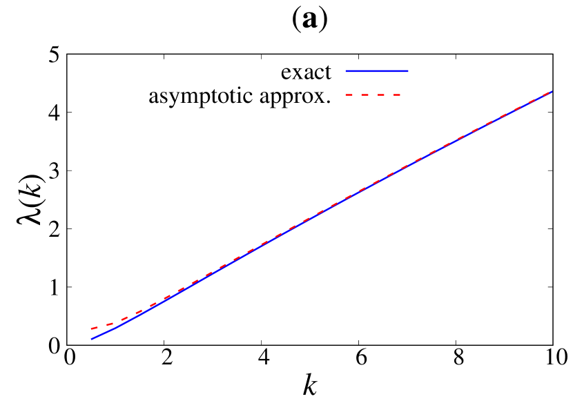
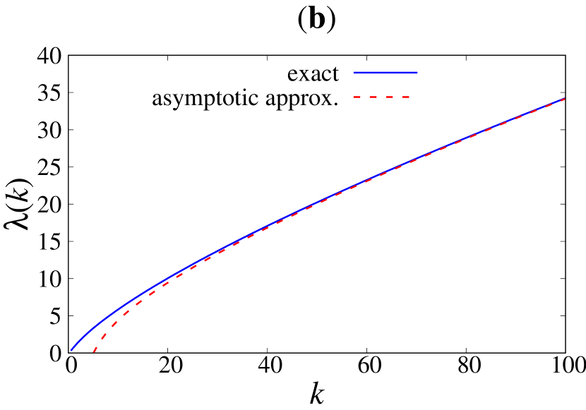
Figure 1: Cumulant generating function $\lambda(k)$, comparing exact value obtained by summation (equation (15) with asymptotic approximation, (25). (a): $\tau_{n}=n^{-4/3}$, ${\cal N}=10^{4}$. (b): $\tau_{n}=n^{-4/3}[1+(n/\tilde{n})^{-2/3}\exp(-n/\tilde{n})]$, $\tilde{n}=3$, ${\cal N}=10^{4}$.

Figure 2 compares different approaches to determining the PDF, $p(T)$, of the time taken to reach size ${\cal N}$. These are

1. Evaluation by simulation using ${\cal M}=10^{8}$ realisations of equation (1).

2. Numerical evaluation of the Bromwich integral, equations (15), (16).

3. Saddle point approximation, equation (18), with the cumulant generating function $\lambda(k)$ evaluated using the asymptotic formula (25). The saddle-point equation (19) is solved numerically to determine $k^{\ast}$.

4. Asymptotic approximation, using equation (29).

The two panels show the same cases as figure 1. The first two methods should yield the same results, apart from fluctuations due to finite sample size of the simulation. The results of using the saddle-point approximation and equation (29) are both in excellent agreement in the limit as $t\to 0$.

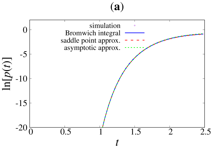
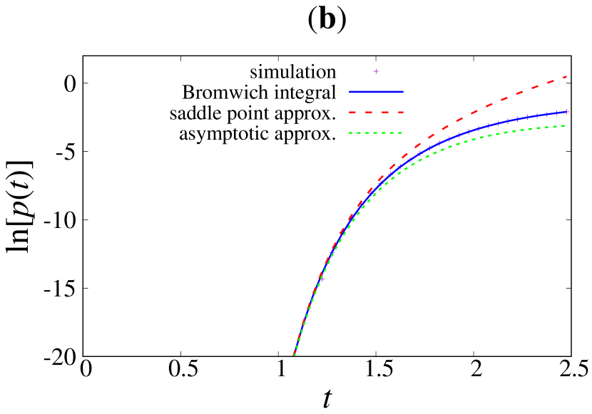
Figure 2: Comparing different approximations for the PDF $p(t)$ of the time taken for ${\cal N}$ collisions, according to the model (1). Simulations and the Bromwich integral (15) agree precisely. The saddle-point approximation (18) and equation (29) are in excellent agreement when $\tau_{n}=n^{-4/3}$, ${\cal N}=10^{4}$ (case (a)), and asymptotic to these other curves as $t\to 0$ when $\tau_{n}=n^{-4/3}[1+(n/\tilde{n})^{-2/3}\exp(-n/\tilde{n})]$, $\tilde{n}=3$, ${\cal N}=10^{4}$ (case (b)).

Figure 3 compares estimates of $P(t)$ obtained by simulation (using $10^{7}$ realisations of (1)) with the result of the asymptotic formula, (31), for a combination of parameter values which differs from figures 1 and 2. Again, there is good agreement as $t\to 0$. A notable feature of the figures 2 and 3 is that changing the rates of the initial collisions has very little effect. For example, comparing figure 3(b) and figure 2(a), the mean time for the first collision, $\tau_{1}$, is increased by a factor of $1+4^{2/3}=3.519\ldots$, and the total number of collisions is increased to ${\cal N}=10^{5}$ from ${\cal N}=10^{4}$, but the intercept on the $t$ axis is only shifted by a small factor.

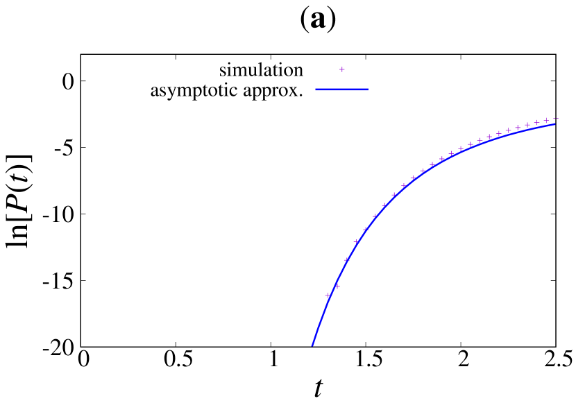
Figure 3: Comparing a simulation the probability $P(t)$ for a droplet to reach ${\cal N}$ collisions after time $t$, with its asymptotic approximation, (31): $\tau_{n}=n^{-4/3}[1+(n/\tilde{n})^{-2/3}\exp(-n/\tilde{n})]$, with (a): $\tilde{n}=2$, ${\cal N}=10^{5}$, (b) $\tilde{n}=4$, ${\cal N}=10^{5}$.

3.4 Implications for rainfall

Section 2 gave an equation, (13), which gives an upper bound on the time $T^{\ast}$ to produce a rain shower, which removes a fraction greater than $\mu$ of the liquid water content of a cloud, subject to the constraint that the fraction of un-collided droplets is always greater than $\nu$ up until time $T^{\ast}$. Making use of this upper bound in the general case would require a complicated calculation, but there is a limiting case where (13) can be replaced by a simpler relation, equation (3). This is realised if the time $T^{\ast}$ is sufficiently small that the fraction of un-collided droplets remains close to unity up to time $T^{\ast}$. At short times, the first collision of a droplet is almost always with another un-collided droplet, so that the fraction of un-collided droplets at time $t$ is approximated by

$$\nu(t)=1-\frac{t}{\tau_{1}}+O(t^{2})$$ (32)

so that if the solution of (3) satisfies $T^{\ast}/\tau_{1}\ll 1$, then the use of this simplified equation (3) to estimate $T^{\ast}$ is justified.

Now that the large-deviation rate function is available from equation (31), it is possible to estimate the ratio $T^{\ast}/\tau_{1}$ and establish when the use of the simplified equation (3) is indeed justifiable (implying that a shower can occur in a timescale which is much shorter than the mean time for the first collision). From (31), the rate function may be written in the form

$${\cal J}(T)=\alpha(\gamma)+\Sigma_{1}+\frac{1}{2}\ln\left(\frac{\tilde{T}}{T_{0}}\right)+\left(\frac{\tilde{T}}{T_{0}}\right)^{-\frac{1}{\gamma-1}}$$ (33)

where $\tilde{T}$ is defined by (27), $\alpha(\gamma)$ is independent of $\tilde{T}$ and

$$T_{0}(\gamma)=\left[A(\gamma)\right]^{\gamma}(\gamma-1)^{\gamma-1}\ .$$ (34)

In the important case where $\gamma=4/3$, $A(4/3)=3\pi/2\sqrt{2}$, $T_{0}(4/3)=3.4508\ldots$ and $\alpha(4/3)=-0.38018\ldots$. Another case, for comparison, is $\gamma=2$, where $A(2)=\pi/2$, $T_{0}(2)=2.4674\ldots$ and $\alpha(2)=-0.81398\ldots$.

Now consider using these results to estimate $T^{\ast}$ by approximating the solution of (3). An instructive approach is to approximate the rate function by ${\cal J}(t)\approx\Sigma_{1}+(t/T_{0})^{-1/(\gamma-1)}$, so that the solution to (3) is approximated by

$$T^{\ast}\sim T_{0}\left[\ln({\cal N}-\Sigma_{1})\right]^{-(\gamma-1)}$$ (35)

where ${\cal N}\approx 10^{6}$ is the number of microscopic droplets which coalesce to form a raindrop, and where $\Sigma_{1}$ is defined by equation (26). Note that this estimate for $T^{\ast}$ is rather insensitive to the rates of the first few collisions (which only enter through the quantity $\Sigma_{1}$). This estimate for $T^{\ast}$ is to be compared with the timescale for the first collision, $\tau_{1}$, as specified by equation (4), so that

$$\frac{T^{\ast}}{\tau_{1}}\approx\frac{T_{0}}{1+Q(1/\tilde{n})}\left[\ln{\cal N}-\Sigma_{1}\right]^{-(\gamma-1)}\ .$$ (36)

In the case where the collision times follow a simple power-law, $\tau_{n}=n^{-\gamma}$, and $Q(x)=\Sigma_{1}=0$, the ratio $T^{\ast}/\tau_{1}$ is not a small number when $\gamma=4/3$ and ${\cal N}=10^{6}$: in that case equation (36) gives $\frac{T^{\ast}}{\tau_{1}}\approx 1.438$, and a numerical solution of (3) yields $\frac{T^{\ast}}{\tau_{1}}\approx 1.381$. If, however, the first few collisions are much slower, this has a small effect on $T^{\ast}$, while $\tau_{1}$ can be greatly increased. For example, if ${\cal N}=10^{6}$ and $\tau_{n}=n^{-4/3}[1+(n/\tilde{n})^{-2/3}\exp(-n/\tilde{n})]$, with $\tilde{n}=5$, then $\Sigma_{1}=4.3671\ldots$ and equation (36) gives $\frac{T^{\ast}}{\tau_{1}}\approx 0.428$, which is a fair approximation to the ratio obtained by a numerical solution of (3), which yields $\frac{T^{\ast}}{\tau_{1}}\approx 0.460$. Because this ratio is less than unity, using the simplified condition, equation (3) should give a fair approximation to the time taken to produce a rain shower. While it would be possible to make a more accurate estimate, the uncertainties arising from this estimate are less than those which are inherent in the model.

4 Distribution of time for passing through size $N$

A cluster that undergoes runaway growth in time $T$ must pass through size $N$ (with $N<{\cal N}$), which is reached at some intermediate time $t_{N}<T$. The probability to undergo runaway growth in time $T$ may be written

$$P(T)=\int_{0}^{T}{\rm d}t_{1}\int_{0}^{t_{1}}{\rm d}t_{2}\ p^{<}_{N}(t_{2})p^{>}_{N}(t_{1}-t_{2})$$ (37)

where $p^{<}_{N}(t)$ is the PDF for a cluster to grow from size $1$ to size $N$ in time $t$ and $p^{>}_{N}(t)$ is the PDF to grow from $N$ to ${\cal N}$ in time $t$. Thus

$$p(t)=\int_{0}^{t}{\rm d}t^{\prime}\ p^{<}_{N}(t^{\prime})p^{>}_{N}(t-t^{\prime})$$ (38)

is the probability density to have undergone runaway growth in time $t$. When $t$ is small, both of the probability densities $p^{>}_{N}$ and $p^{<}_{N}$ are very small, and can be addressed by large deviation theory: write

$$p^{<}_{N}(t)=\exp[-{\cal J}^{<}_{N}(t)]\ ,\ \ \ p^{>}_{N}(t)=\exp[-{\cal J}^{>}_{N}(t)]\ .$$ (39)

In this limit it is, therefore, expected that the distribution $p^{<}_{N}(t^{\prime})p^{>}_{N}(t-t^{\prime})$ is very sharply peaked, with the maximum with respect to $t^{\prime}$ at a point $t_{N}^{\ast}$. It is expected that those clusters which reach size ${\cal N}$ in a short time $T$ pass through size $N$ at a time which is close to $t_{N}^{\ast}$. This time $t^{\ast}_{N}$ is well approximated by the position of the minimum of

$$F_{N}(t)={\cal J}^{<}_{N}(t)+{\cal J}^{>}_{N}(T-t)\ .$$ (40)

Now consider, in succession, the problem of determining the functions ${\cal J}^{>}_{N}$ and ${\cal J}^{<}$, before estimating $t^{\ast}_{N}$.

To avoid over-complicated notation, this calculation will be carried out when the $\tau_{n}$ are a simple power-law: $\tau_{n}=n^{-\gamma}$.

4.1 Runaway growth: $N$ to ${\cal N}$

For power-law mean collision time $\tau_{n}=n^{-\gamma}$, the cumulant generating function for growth from $N$ to $\infty$ is

$$\lambda^{>}_{N}(k)=\sum_{n=N}^{\cal N}\ln\left(1+kn^{-\gamma}\right)\ .$$ (41)

If $N=1$, this is well approximated by equation (21). Assuming that $kN^{-\gamma}\ll 1$, subtracting the sum from $1$ to $N$ gives

$$\lambda^{>}_{N}(k)\sim\gamma A(\gamma)k^{1/\gamma}-\left(N-\frac{1}{2}\right)\ln k-\gamma{\cal C}-\sigma_{N}-k\frac{{\cal N}^{-(\gamma-1)}}{\gamma-1}$$ (42)

with

$$\sigma_{N}=\sum_{n=1}^{N-1}\ln\tau_{n}\ .$$ (43)

Following the approach described in section 3, inverting the Laplace transform using a Bromwich integral, and approximating this using a saddle point (Laplace) approximation gives

$$p^{>}_{N}(t)=\frac{1}{\sqrt{2\pi|{\lambda^{>}_{N}}^{\prime\prime}(k^{\ast})|}}\exp[-J^{>}_{N}(k^{\ast})]\ .$$ (44)

The saddle point $k^{\ast}$ satisfies

$$t=\frac{{\rm d}\lambda^{>}}{{\rm d}k}(k^{\ast})\ ,\ \ \ \frac{{\rm d}}{{\rm d}k}\lambda_{N}^{>}(k)=Ak^{(1-\gamma)/\gamma}-\frac{N-\frac{1}{2}}{k}-\frac{{\cal N}^{-(\gamma-1)}}{\gamma-1}$$ (45)

and $J^{>}_{N}(k)=\lambda^{>}_{N}(k)-k\lambda^{\prime>}_{N}(k)$. The solution is, at leading order in $1/k$,

$$k^{\ast}\sim b\tilde{t}^{-1/(\gamma-1)}\left(1-\frac{\gamma(N-\frac{1}{2})}{(\gamma-1)b}\tilde{t}^{1/(\gamma-1)}\right)\ ,\ \ \ \tilde{t}=t+\frac{{\cal N}^{-(\gamma-1)}}{\gamma-1}$$ (46)

and $b$ is given by (30). Noting that $Ab^{1/\gamma}=b$, and expressing $J_{N}$ as a function of $t$ by writing $J_{N}(t)=J_{N}(k^{\ast}(t))$ gives

$$J^{>}_{N}(\tilde{t}) = (\gamma-1)b\tilde{t}^{-1/(\gamma-1)}+\frac{\gamma}{\gamma-1}\left(N-\frac{1}{2}\right)\ln\tilde{t}$$ (47)

$$-\left(N-\frac{1}{2}\right)\ln b-\gamma{\cal C}-\sigma_{N}$$

and hence

$$p^{>}_{N}(\tilde{t})\sim\sqrt{\frac{\gamma}{2\pi(\gamma-1)}}b^{N}\exp[\gamma{\cal C}+\sigma_{N})]\tilde{t}^{-\frac{\gamma(2N+1)-1}{2(\gamma-1)}}\exp\left(-(\gamma-1)b\tilde{t}^{-1/(\gamma-1)}\right)\ .$$ (48)

Upon setting $N=1$, this result is in agreement with (29) when $\Sigma_{1}=0$. Figure 4 compares equation (48) with exact evaluation of $p^{>}_{N}(t)$ (simulation and evaluation of the Bromwich integral), and with the saddle point approximation, with $\gamma=4/3$ and ${\cal N}=10^{4}$, for $N=2$ (a) and $N=3$ (b).

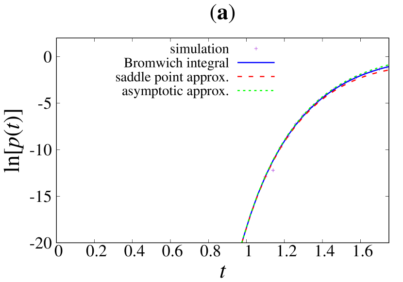
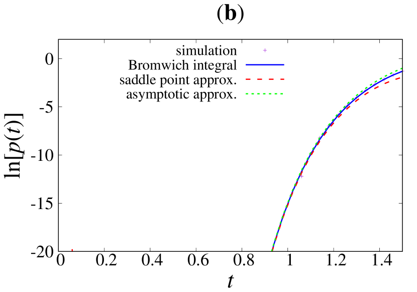
Figure 4: Comparing equation (48) with simulation, the Bromwich integral (15), and saddle-point approximation (18). For both panels, $\tau_{n}=n^{-4/3}$, ${\cal N}=10^{4}$. (a): $N=2$, (b): $N=3$.

4.2 Initial growth: $1$ to $N-1$

Now estimate the probability density $p^{<}_{N}(t)$ to undergo the first $N-1$ collisions in time $t$, using the same approach. The cumulant generating function is

$$\lambda^{<}_{N}(k)=\sum_{n=1}^{N-1}\ln\left(1+kn^{-\gamma}\right)\ .$$ (49)

To leading order in $k^{-1}$, this is

$$\lambda^{<}_{N}(k)\sim(N-1)\ln k-\sigma_{N}$$ (50)

where $\sigma_{N}$ was defined in (43). The saddle point satisfies

$$t=\frac{{\rm d}\lambda^{<}_{N}}{{\rm d}k}(k^{\ast})$$ (51)

so that

$$k^{\ast}=\frac{N-1}{t}$$ (52)

and hence $\frac{{\rm d}^{2}\lambda^{<}_{N}}{{\rm d}k^{2}}(k^{\ast})=-t^{2}/(N-1)$. As a function of $t$, at leading order,

$$J^{<}_{N}(t)\sim-(N-1)\ln t+(N-1)\left[\ln(N-1)-1\right]+\sigma_{N}$$ (53)

so that

$$p^{<}_{N}(t)\sim\sqrt{\frac{N-1}{2\pi}}\exp\left[-\sigma_{N}-(N-1)\left(\ln(N-1)-1\right)\right]t^{N-2}\ .$$ (54)

Figure 5 compares equation (54) with exact evaluation on $p^{<}_{N}(t)$ (simulation and evaluation of the Bromwich integral), and with the saddle point approximation, with $\gamma=4/3$ and ${\cal N}=10^{4}$, for $N=2$ (a) and $N=3$ (b).

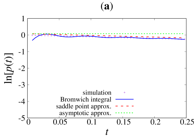
Figure 5: Comparing equation (54) with simulation, the Bromwich integral (15), and saddle-point approximation (18). For both panels, $\tau_{n}=n^{-4/3}$, ${\cal N}=10^{4}$. (a): $N=2$, (b): $N=3$.

4.3 Growth history of lucky drops

The forms of the functions ${\cal J}^{<}_{N}$ and ${\cal J}^{>}_{N}$ can now be identified. Ignoring irrelevant constant terms, the function defined in (40) is

$$F_{N}(\tilde{t}) = -(N-2)\ln\left(\tilde{t}-\frac{{\cal N}^{-(\gamma-1)}}{\gamma-1}\right)+b(\gamma-1)(T-\tilde{t})^{-1/(\gamma-1)}$$ (55)

$$+\frac{\gamma(2N+1)-1}{2(\gamma-1)}\ln(T-\tilde{t})$$

where $\tilde{t}$ was defined in (46). Note that there are two terms which are functions of $T-\tilde{t}$, and that in the limit as $T\to 0$, the power-law term is dominant over the logarithmic term. Ignoring the term in $\ln(T-\tilde{t})$, and differentiating the remaining terms with respect to $\tilde{t}$

$$F^{\prime}_{N}(\tilde{t})\sim b(T-\tilde{t})^{-\gamma/(\gamma-1)}-\frac{(N-2)}{\tilde{t}-{\cal N}^{-(\gamma-1)}/(\gamma-1)}$$ (56)

so that, if $t_{N}/T\ll 1$, the minimum of $F_{N}(t)$ is at

$$t_{N}^{\ast}\sim\frac{N-2}{b}T^{\gamma/(\gamma-1)}+\frac{{\cal N}^{-(\gamma-1)}}{\gamma-1}\ .$$ (57)

This implies that, for those ‘lucky’ droplets that do undergo runaway growth, the typical value $t^{\ast}_{N}$ of the time when they have undergone $N$ collisions is initially increasing linearly with $N$, regardless of the value of the exponent $\gamma$. This is a surprising result. It is, however, consistent with the observations made in section 3, that the growth time of the fast-growing droplets is not strongly influenced by the first few values of the $\tau_{n}$.

The approximation (57) breaks down when the predicted value of $t^{\ast}_{N}$ is no longer small compared to $T$. This occurs after $N^{\ast}$ collisions, where $N^{\ast}\sim bT^{-1/(\gamma-1)}$.

The history of the fastest growing droplets was investigated numerically. The growth process represented by (1) was simulated for ${\cal M}$ realisations, and the random number seeds for the $K$ realisations where the sum (1) is less than $T$ were recorded. These $K$ cases were run again, and their growth history $N(t)$ was recorded (where $N$ is the size of the cluster at time $t$). Figure 6 plots the mean size $\langle N(t)\rangle$ (and also the median size) of these $K$ clusters, which represent the $K/{\cal M}$ fraction which exhibits the fastest growth. Simulations with $\tau_{n}=n^{-\gamma}$, for two different values of $\gamma$, both show a linear initial growth. The mean value $\langle N(t)\rangle$ is compared with the prediction

$$\langle N(t)\rangle\sim bT^{-\gamma/(\gamma-1)}t+{\rm const.}\ .$$ (58)

obtained from equation (57), and good agreement is observed.

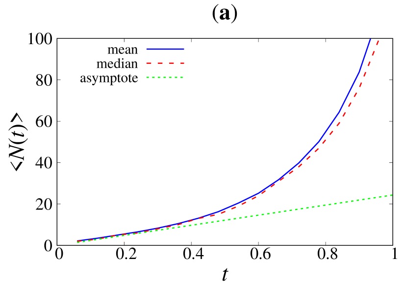
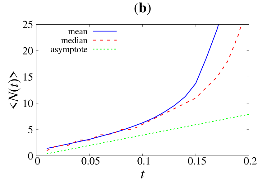
Figure 6: Plot of mean particle size $\langle N(t)\rangle$ for the fraction $K/{\cal M}\approx P(T)$ of fastest growing particles, which reach size ${\cal N}$ in time less than $T$. (a): $\gamma=4/3$, $T=1.5$, $P(T)=1.884\ldots\times 10^{-4}$, ${\cal N}=10^{4}$. (b): $\gamma=2$, $T=0.25$, $P(T)=3.681\ldots\times 10^{-4}$, ${\cal N}=10^{4}$. In both cases the number of realisations of equation (1) was ${\cal M}=10^{6}$.

5 Conclusions

The slow rate of collision between microscopic droplets in ice-free (‘warm’) clouds appears to impose a severe difficulty in explaining the rapid onset of rain showers. However, this difficulty may be overcome by recognising that, because a raindrop is the result of coalescence of roughly a million microscopic droplets, a rain shower is created by the one-in-a-million fraction of droplets which have the fastest growth.

Reference Wil16 proposed a surprisingly simple equation, (3), for determining the time taken for the onset of a rain shower. This work has developed the arguments supporting equation (3) in greater detail. It has also shown how the function ${\cal J}(T)$ can be approximated in cases where the mean collision times $\tau_{n}$ have a much more general dependence on $n$ than the simple power-law considered in Wil16 . The probability $P(t)$ for undergoing ${\cal N}$ collisions in time $t$ is given by an explicit asymptotic expression, equation (31), which is valid for a rather general form of the collision times $\tau_{n}$. This formula implies that the timescale for the onset of a rain shower can be short compared to the mean time for even the first of the million collisions.

Equation (31) allows a quantitative application to understanding rainfall from a homogeneous atmosphere. However, its principal significance for meteorology may be qualitative rather than quantitative, in that it implies that the apparent kinetic barrier to making rainfall from warm clouds is of little significance, even for a homogeneous atmosphere. In practice, the atmosphere may contain a sufficiently large fraction of unusual nucleation centres, which nucleate atypically large microscopic droplets. It is these larger droplets which are likely to become raindrops.

While not readily experimentally observable, it is of interest to understand the growth history of those rare, fast-growing droplets that do become raindrops. Rather surprisingly, they are found to initially grow linearly as a function of time, irrespective of the $n$-dependence of the mean collision times, $\tau_{n}$.

The datasets generated during and/or analysed during the current study are available from the corresponding author on reasonable request.

References

- (1) B. J. Mason, The Physics of Clouds, 2nd. ed., Oxford, University Press, (1971).
- (2) H. R. Pruppacher and J. D. Klett, Microphysics of Clouds and Precipitation, 2nd ed., Dordrecht, Kluwer, (1997).
- (3) R. A. Shaw, Particle-turbulence interactions in atmospheric clouds, Ann. Rev. Fluid Mech., 35, 183-227, (2003).
- (4) E. M. Lifshitz and V. V. Slyozov, J. Phys. Chem. Solids, 19, 35, (1961)
- (5) E. M. Lifshitz and L. P. Pitaevskii, Physical kinetics, Pergamon, Oxford, (1981).
- (6) C. F. Clement, Environmental Chemistry of Aerosols (Blackwell Publishing, Oxford), p. 49–89, (2008).
- (7) M. Wilkinson, A Test-Tube Model for Rainfall, Europhys. Lett., 106, 40001, (2014).
- (8) P. G. Saffamn and J. S. Turner, On the collision of drops in turbulent clouds, J. Fluid Mech., 1, 16-30, (1956).
- (9) A. Pumir and M. Wilkinson, Collisional Aggregation due to Turbulence, Ann. Rev. Cond. Matter Phys., 7, 141-70, (2016).
- (10) J. W. Telford, A new aspect of coalescence theory, J. Meteor., 12, 436?44, (1955).
- (11) S. Twomey, Computations of rain formation by coalescence, J. Atmos. Sci., 23, 405?11, (1966).
- (12) A.B. Kostinski and R.A. Shaw, Fluctuations and luck in droplet growth by coalescence, Bull. Am. Met. Soc., 86, 235-244, (2005).
- (13) M. Wilkinson, Large Deviation Analysis of Rapid Onset of Rain Showers, Phys. Rev. Lett., 116, 018501, (2016).
- (14) M. I. Freidlin and A. D. Wentzell, Random Perturbations of Dynamical Systems, Grundlehren der Mathematischen Wissenschaften, vol. 260, Springer, New York, (1984).
- (15) H. Touchette, The large deviation approach to statistical mechanics, Phys. Rep., 478, 1-69, (2009).
- (16) M. Smoluchowski, Drei Vorträge über Diffusion, Brownsche Molekularbewegung und Koagulation von Kolloidteilchen, Phys. Z. , 17, 585–99, (1916).
- (17) D. J. Aldous, Deterministic and stochastic models for coalescence (aggregation and coagulation): a review of the mean-field theory for probabilists, Bernoulli, 5, 3–48, (1999).
- (18) P. van Dongen, On the possible occurrence of instantaneous gelation in Smoluchowski’s coagulation equation, J. Phys. A: Math. Gen., 20, 1889-1904, (1987).
- (19) F. Leyvraz, Scaling theory and exactly solved models in the kinetics of irreversible aggregation, Phys. Rep., 383, 95-212, (2003).
- (20) R. C. Ball, C. Connaughton, T. H. M. Stein and O. Zaboronski, Instantaneous gelation in Smoluchowski’s coagulation equation revisited, Phys. Rev. E, 84, 011111, (2011).