An efficient semismooth Newton-AMG-based inexact primal-dual algorithm for generalized transport problems

Abstract

This work is concerned with the efficient optimization method for solving a large class of optimal mass transport problems. An inexact primal-dual algorithm is presented from the time discretization of a proper dynamical system, and by using the tool of Lyapunov function, the global (super-)linear convergence rate is established for function residual and feasibility violation. The proposed algorithm contains an inner problem that possesses strong semismoothness property and motivates the use of the semismooth Newton iteration. By exploring the hidden structure of the problem itself, the linear system arising from the Newton iteration is transferred equivalently into a graph Laplacian system, for which a robust algebraic multigrid method is proposed and also analyzed via the famous Xu–Zikatanov identity. Finally, numerical experiments are provided to validate the efficiency of our method.

Keywords: Optimal transport, primal-dual method, Lyapunov function, semismooth Newton iteration, graph Laplacian, algebraic multigrid, Xu–Zikatanov identity

1 Introduction

The optimal mass transport proposed by Monge, can be dated back to as early as the 1780s. Later, Kantorovich [46] introduced a convex relaxation of Monge’s original formulation and applied it to economics. Since then, this topic attracted more attentions and it also played an increasing role in imaging processing [42, 67, 77], machine learning [3, 29, 45] and statistics [71, 80]. We refer the readers to [82, 83] for comprehensive theoretical investigations.

In the discrete setting, Kantorovich’s relaxation (cf.2), which is also known as the Monge–Kantorovich problem [15], seeks an optimal transfer plan (an $n$-by-$n$ nonnegative matrix) that minimizes the total transport cost between two given mass distributions in the $n$-dimensional probability simplex. Except for this classical formulation, nowadays, there are some extensions, such as partial optimal mass transport [19] and capacity-constrained transport problem [48]. All these transport-like programmings share the common feature of marginal constraint and can be formulated as standard but large scale linear programmings (LP); see Section 2 for more details. Besides, entropy regularization, i.e., the logarithmic barrier function, has been used to relax the nonnegative restriction and provides an approximate optimization problem that possesses some nice properties including strong convexity of the primal form (which corresponds to the smoothness of the dual problem) and closed projection onto the marginal constraint.

Let us first review some existing methods based on entropy regularization. The well-known Sinkhorn algorithm [30, 79] and its greedy adaptation, called Greenhorn [2], are fixed-point type iterations. Sinkhorn’s algorithm was proved to converge linearly (cf. [69, Theorem 35]) but the rate is exponentially degenerate with respect to the regularization parameter, and the theoretical complexity bound $\mathcal{O}(n^{2}/\epsilon^{2})$ can be found in [32, 60]. Here, we mention that the iterative Bregman projection [8] with Kullback–Leibler divergence is equivalent to Sinkhorn’s algorithm. By virtue of the smoothness of the dual problem, accelerated mirror descent methods have been proposed in [32, 60], and the provable complexity is $\mathcal{O}(n^{2.5}\sqrt{\ln n}/\epsilon)$. For more methods using the entropy regularization, we refer to [25, 38, 40], and one can also consult [7, 69, 73] on quite complete surveys about numerical methods.

It is worth noticing that, the solution to the entropy regularized problem exists uniquely, and as the regularization parameter vanishes, it converges (exponentially) to an optimal transport plan with maximal entropy among all the optimal plans; see [28] and [73, Proposition 4.1]. However, practically, one cannot choose arbitrarily small parameters due to the round-off issue and instability effect. That being said, the log-domain technique [26] enhances the stability, and both vectorization and parallelization can be applied to Sinkhorn’s algorithm.

The complexity of matrix-vector multiplication in each iteration of the Sinkhorn algorithm is $\mathcal{O}(n^{2})$ for general cases. If the transport cost function enjoys a separable structure with $d$ blocks, then efficient implementation achieves the reduced cost $\mathcal{O}(n^{1+1/d})$; see [73, Section 4.3]. More recently, for translation invariance cost functions (for instance, the Euclidean distance) that imply the cyclic property, Liao et al. [57] proposed an optimal $\mathcal{O}(n)$ algorithm. Hence, to provide an approximate optimal transport plan with moderate regularization parameter, entropy-based methods are efficient, especially for some cost functions with nice properties. This makes them very popular in real applications, especially for computing Wasserstein distances between histograms.

On the other hand, augmented Lagrangian method (ALM) and alternating direction method of multipliers (ADMM) can be applied to transport-like problems as well. By the celebrated stability result of linear inequality system [68, 76], we have global linear convergence for ADMM [33]. For general convex objectives, the provable nonergodic rate of many accelerated variants of (linearized) ALM and ADMM is $\mathcal{O}(1/k)$; see [54, 63, 64, 91]. The method [91, Algorithm 1] possesses a faster sublinear rate $\mathcal{O}(1/k^{2})$ but involves a large scale quadratic programming (of dimension $n^{2}$) of the primal variable.

There are also classical LP solvers such as the interior-point method [50, 72] and semismooth Newton-based algorithms [4, 13, 55, 61]. These methods have to solve a symmetric positive definite (SPD) system per (inner) iteration, and prevailing linear solvers are (sparse) Cholesky decomposition and preconditioned conjugate gradient (PCG). However, the corresponding SPD system might be nearly singular and ill-conditioned as the problem size increases, and thus the number of iterations grows dramatically. Therefore, efficient and robust linear solvers play important roles in these algorithms. We also refer the readers to [1, 9, 73] for some combinatorial methods.

1.1 Main results

In this work, we propose an efficient inexact primal-dual method for the generalized transportation problem (cf.6), which includes a large class of transport-like programmings, such as optimal mass transport, partial optimal transport, and capacity-constrained transport problem. Our algorithm is based on proper time discretization of the accelerated primal-dual dynamical system [63] and adopts the semismooth Newton (SsN) iteration as the inner solver.

In the setting of inexact computations, we prove the contraction estimate

$$\mathcal{E}_{k+1}-\mathcal{E}_{k}\leq-\alpha_{k}\mathcal{E}_{k+1},$$

where $\alpha_{k}>0$ is the step size and $\mathcal{E}_{k}$ denotes the discrete Lyapunov function (cf.17). Besides, we establish the global convergence rate of the objective residual and the feasibility violation (see Theorem 2):

$$h(x_{k})-h(x^{*})+\left\lVert{Gx_{k}+I_{Y}y_{k}+I_{Z}z_{k}-b}\right\rVert\leq C\prod_{i=0}^{k-1}\frac{1}{1+\alpha_{i}}.$$

This implies linear rate as long as $\alpha_{k}\geq\alpha>0$ and superlinear convergence follows if $\alpha_{k}\to+\infty$. See Remarks 3 and 4 for detailed discussions.

The inner problem (cf.14) is a nonlinear equation with strongly semismooth property. This motivates us to adopt the SsN iteration, which requires solving an $N$-by-$N$ linear SPD system

(1) $$\mathcal{T}\xi=\left(\epsilon I+T\Lambda T^{\top}\right)\xi=z,$$

where $\Lambda$ is diagonal and $\epsilon>0$ is a small number. Utilizing the hidden structure of $\mathcal{T}$, we transfer it equivalently into $A=\epsilon D+A_{0}$, where $D$ is diagonal and $A_{0}$ is the Laplacian matrix of a bipartite graph, and then develop a robust algebraic multigrid (AMG) algorithm. Invoking the well-known Xu–Zikatanov identity [89], we prove the convergence rate of the two-level case (see Theorem 7):

$$\left\lVert{\xi_{i+1}-\xi^{*}}\right\rVert_{A}=\left(1-\frac{1}{c_{1}}\right)\left\lVert{\xi_{i}-\xi^{*}}\right\rVert_{A},\quad\,c_{1}\leq C+\frac{1}{1-\left\lVert{I-\bar{R}_{c}A_{c}}\right\rVert_{A_{c}}},$$

where $\bar{R}_{c}$ and $A_{c}$ are respectively the coarse level solver and coarse level matrix, and $C\geq 1$ is independent of the number $\epsilon$ and the problem size $N$.

1.2 Outline

The rest of this paper is organized as follows. In Section 2, we give the problem setting and introduce the generalized transportation problem. After that, in Section 3, we present our inexact SsN-based primal-dual method and prove the global convergence rate via a discrete Lyapunov function. Then, in Section 4, we focus on the linear SPD system arising from the SsN iteration and transfer it into an equivalent graph Laplacian system, for which a robust and efficient AMG algorithm is proposed and analyzed in Sections 5 and 6, respectively. We provide several numerical tests in Section 7 to show the robustness of the AMG algorithm and the performance of our overall SsN-AMG-based inexact primal-dual method. Finally, we conclude our work in Section 8.

2 Problem Setting

In this part, we list several typical transport-like programmings arising from either mathematical extensions or practical applications. Those problems share the common feature of marginal constraint and will be treated in a unified way.

2.1 Transport-like problems

2.1.1 Optimal transport

In the setting of optimal mass transportation [15, 46], we are given a cost matrix $C\in\,{\mathbb{R}}^{m\times n}_{+}$ and two vectors $\mu\in\,{\mathbb{R}}^{n}_{+},\,\nu\in\,{\mathbb{R}}_{+}^{m}$ satisfying the mass conservation condition: ${\bf 1}_{n}^{\top}\mu={\bf 1}_{m}^{\top}\nu$, and aim to solve the minimization problem

(2) $$\min_{X\in\mathcal{B}(\mu,\nu)}\,\left\langle{C,X}\right\rangle:=\sum_{i=1}^{m}\sum_{j=1}^{n}C_{ij}X_{ij},$$

where $\mathcal{B}(\mu,\nu):=\left\{X\in\,{\mathbb{R}}^{m\times n}_{+}:\,X^{\top}{\bm{1}}_{m}=\mu,\,X{\bm{1}}_{n}=\nu\right\}$ denotes the transportation polytope, with ${\bm{1}}_{n}({\bf 1}_{m})\in\,{\mathbb{R}}^{n}(\,{\mathbb{R}}^{m})$ being the vector of all ones. According to [17, Chapter 8], $\mathcal{B}(\mu,\nu)$ is nonempty, convex and bounded. It follows immediately from [10, Corollary 2.3] that 2 admits at least one solution, which is called an optimal transport plan.

When $m=n$ and $\mu=\nu={\bf 1}_{n}$, the transportation polytope coincides with the Birkhoff polytope $\mathcal{B}_{n}:=\{X\in\,{\mathbb{R}}_{+}^{n\times n}:X^{\top}{\bf 1}_{n}={\bf 1}_{n},\,X{\bf 1}_{n}={\bf 1}_{n}\}$, which consists of all $n$-by-$n$ doubly stochastic matrices. The celebrated Birkhoff–Von-Neumann theorem (cf. [69, Theorem 17]) states that $\mathcal{B}_{n}$ is the convex hull of all permutation matrices. Therefore, it has frequently been used to relax some combinatorial or nonconvex problems [37]. In particular, the optimal transport 2 is exactly the convex relaxation of the linear assignment problem [18].

2.1.2 Birkhoff projection

Given any $\Phi\in\,{\mathbb{R}}^{n\times n}_{+}$, the Birkhoff projection in terms of the Frobenius norm $\left\lVert{\cdot}\right\rVert_{F}$ considered in [47, 56] reads as

(3) $$\min_{X\in\mathcal{B}_{n}}\frac{1}{2}\left\lVert{X-\Phi}\right\rVert_{F}^{2},$$

which actually seeks the nearest doubly matrix of $\Phi$ and usually arises from the relaxations of some nonconvex programmings [37, 43, 58]. Besides, in the setting of numerical simulation for circuit networks [5], we have to fix some components:

(4) $$X_{ij}=\Phi_{ij},\quad\forall\,i\in\mathcal{I},\,j\in\mathcal{J},$$

where $\mathcal{I},\,\mathcal{J}\subset\{1,2,\cdots,n\}$ are two given index sets, and this leads to the problem of finding the best approximation in the Birkhoff polytope $\mathcal{B}_{n}$ with prescribed entry constraint [4, 39].

2.1.3 Partial optimal transport

In standard optimal transport 2, the marginal distributions $\mu$ and $\nu$ are required to have the same mass. Mathematically, this is quite restrictive and practically, the unbalanced case ${\bf 1}_{n}^{\top}\mu\neq{\bf 1}_{m}^{\top}\nu$ stems from the positive-unlabeled learning [20] and the representation of dynamic meshes for controlling the volume of objects with free boundaries [66].

This leads to a problem called partial optimal transport [8, 26]. More precisely, we aim to transport only a given fraction of mass $a\in(0,a_{\max}]$ where $a_{\max}:=\min\{{\bf 1}_{n}^{\top}\mu,\,{\bf 1}_{m}^{\top}\nu\}$, and minimize the total cost

(5) $$\min_{X\in\,{\mathbb{R}}_{+}^{m\times n}}\left\langle{C,X}\right\rangle\quad{{\rm s.t.}\,}\,X^{\top}{\bf 1}_{m}\leq\mu,\quad X{\bf 1}_{n}\leq\nu,\quad{\bf 1}_{m}^{\top}X{\bf 1}_{n}=a.$$

When $a=\mu^{\top}{\bf 1}_{n}=\nu^{\top}{\bf 1}_{m}$, this amounts to optimal transport 2. Well-posedness of 5 (in the continuous setting) was established in [19] and extended by Figalli [36].

2.2 Generalized transportation problem

Clearly, the transport plan $X$ belongs to a box region $\mathcal{K}:=\{X\in\,{\mathbb{R}}^{m\times n}:\Theta\leq X\leq\Gamma\}$, where $\Theta,\,\Gamma\in\,{\mathbb{R}}^{m\times n}$ with $0\leq\Theta_{ij}<\infty$ and $\Theta_{ij}\leq\Gamma_{ij}\leq\infty$. Introduce two slack variables $y\in\,{\mathbb{R}}^{n}$ and $z\in\,{\mathbb{R}}^{m}$, together with their feasible regions $\mathcal{Y}=\,{\mathbb{R}}^{n}_{+}$ (or $\{0\}$) and $\mathcal{Z}=\,{\mathbb{R}}^{m}_{+}$ (or $\{0\}$). This allows us to include the unbalanced case ${\bf 1}_{n}^{\top}\mu\neq{\bf 1}_{m}^{\top}\nu$. We also impose the total mass constraint $\pi(X)=a$, where $a\in(0,\min\{{\bf 1}_{n}^{\top}\mu,\,{\bf 1}_{m}^{\top}\nu\}]$ and $\pi:\,{\mathbb{R}}^{m\times n}\to\,{\mathbb{R}}^{r}$ is a linear operator.

Then the generalized transportation problem reads as follows

(6) $$\min_{(X,y,z)\in\Omega}H(X)\quad{{\rm s.t.}\,}X^{\top}{\bf 1}_{m}+y=\mu,\quad X{\bf 1}_{n}+z=\nu,\quad\pi(X)=a,$$

where $\Omega:=\mathcal{K}\times\mathcal{Y}\times\mathcal{Z}$ and $H(X):=\sigma/2\left\lVert{X-\Phi}\right\rVert_{F}^{2}+\left\langle{C,X}\right\rangle$ with $\sigma\geq 0$ and $\Phi\in\,{\mathbb{R}}_{+}^{m\times n}$. This generic formulation contains all problems mentioned previously in Section 2.1, and also includes other transport-like problems such as capacity constrained optimal transport [48] and the machine loading problem [35]. Throughout this paper, assume 6 exists at least one solution $(X^{*},y^{*},z^{*})\in\Omega^{*}$, where $\Omega^{*}$ is the set of all global minimizers.

As usual, denote by ${\rm vec}({\times})$ the vector expanded by the matrix $\times$ by column. Let $h(x):=\sigma/2\left\lVert{x-\phi}\right\rVert^{2}+c^{\top}x$ with $c={\rm vec}({C})$ and $\phi={\rm vec}({\Phi})$, and introduce $\mathcal{X}:=\{x\in\,{\mathbb{R}}^{mn}:\theta_{i}\leq x_{i}\leq\gamma_{i},\,1\leq i\leq mn\}$ with $\theta={\rm vec}({\Theta})$ and $\gamma={\rm vec}({\Gamma})$ . Suppose the linear operator $\pi$ admits a matrix representation $\Pi\in\,{\mathbb{R}}^{r\times mn}$ such that $\pi(X)=\Pi{\rm vec}({X})$ for all $X\in\,{\mathbb{R}}^{m\times n}$. Then, we rearrange 6 as a standard affine constrained optimization problem:

(7) $$\min_{(x,y,z)\in\Sigma}\,h(x)\quad{{\rm s.t.}\,}Gx+I_{Y}y+I_{Z}z=b,$$

where $\Sigma:=\mathcal{X}\times\mathcal{Y}\times\mathcal{Z}$ and

(8) $$G:=\begin{pmatrix}T\\ \Pi\end{pmatrix},\quad T:=\begin{pmatrix}I_{n}\otimes{\bf 1}_{m}^{\top}\\ {\bf 1}_{n}^{\top}\otimes I_{m}\\ \end{pmatrix},\quad I_{Y}:=\begin{pmatrix}I_{n}\\ O\\ O\end{pmatrix},\quad I_{Z}:=\begin{pmatrix}O\\ I_{m}\\ O\end{pmatrix},\quad b:=\begin{pmatrix}\mu\\ \nu\\ a\end{pmatrix}.$$

Clearly, $(X^{*},y^{*},z^{*})\in\Omega^{*}$ if and only if $(x^{*},y^{*},z^{*})\in\Sigma^{*}$ and $x^{*}={\rm vec}({X^{*}})$, where $\Sigma^{*}$ denotes the set of all minimizers of problem 7.

At the end of this section, let us make some conventions. The angle bracket $\left\langle{\cdot,\cdot}\right\rangle$ stands for the usual Euclidean inner product of two vectors. For any SPD matrix $A$, define the $A$-inner product $\left\langle{\cdot,\cdot}\right\rangle_{A}:=\left\langle{A\cdot,\cdot}\right\rangle$ and the induced $A$-norm $\left\lVert{\cdot}\right\rVert_{A}=\sqrt{\left\langle{\cdot,\cdot}\right\rangle_{A}}$. When no confusion arises, the $A$-norm of a matrix $B$ is denoted by $\left\lVert{B}\right\rVert_{A}:=\sup_{x\neq 0}\left\lVert{Bx}\right\rVert_{A}/\left\lVert{x}\right\rVert_{A}$. The proximal mapping ${\bf prox}_{\eta g}:\,{\mathbb{R}}^{n}\to\,{\mathbb{R}}^{n}$ of a properly closed convex function $g$ with $\eta>0$ is

$${\bf prox}_{\eta g}(x):=\mathop{{\mathop{{\rm argmin}}\,}}_{y\in\,{\mathbb{R}}^{n}}\left\{g(y)+\frac{1}{2\eta}\left\lVert{y-x}\right\rVert^{2}\right\}\quad\forall\,x\in\,{\mathbb{R}}^{n}.$$

Let $\delta_{\mathcal{O}}(\cdot)$ be the indicator function of a nonempty closed convex subset $\mathcal{O}\subset\,{\mathbb{R}}^{n}$ and define the normal cone at $x$ as follows

$$\mathcal{N}_{\mathcal{O}}(x):=\left\{z\in\,{\mathbb{R}}^{n}:\left\langle{z,x-y}\right\rangle\geq 0\quad\forall\,y\in\mathcal{O}\right\}.$$

For simplicity, we also write ${\rm proj}_{\mathcal{O}}={\bf prox}_{\eta\delta_{\mathcal{O}}}$ for all $\eta>0$.

3 An Inexact SsN-based Primal-Dual Method

For any $\lambda\in\,{\mathbb{R}}^{m+n+r}$ and $\bm{u}=(x,y,z)\in\,{\mathbb{R}}^{mn}\times\,{\mathbb{R}}^{n}\times\,{\mathbb{R}}^{m}$, define the Lagrangian function for 7:

(9) $$\mathcal{L}(\bm{u},\lambda):=h(x)+\delta_{\Sigma}(\bm{u})+\left\langle{\lambda,H\bm{u}-b}\right\rangle,$$

where $H=(G,I_{Y},I_{Z})$. Notice that $\mathcal{L}(\cdot,\lambda)$ is convex and we set $\partial_{\bm{u}}\mathcal{L}(\bm{u},\lambda):=\nabla h(\bm{u})+\mathcal{N}_{\Sigma}(\bm{u})+H^{\top}\lambda$, where $\nabla h(\bm{u})=\sigma(x,{\bf 0}_{n},{\bf 0}_{m})-\widetilde{c}$ with $\widetilde{c}=(\sigma\phi-c,{\bf 0}_{n},{\bf 0}_{m})$.

3.1 An inexact primal-dual algorithm

Let us start from the accelerated primal-dual flow dynamics proposed in [63]:

(10) $$\left\{\begin{aligned} \beta\lambda^{\prime}={}&\nabla_{\lambda}\mathcal{L}(\bm{v},\lambda),\\ \bm{u}^{\prime}={}&\bm{v}-\bm{u},\\ \beta\bm{v}^{\prime}\in{}&-\partial_{\bm{u}}\mathcal{L}(\bm{u},\lambda),\end{aligned}\right.$$

where $\beta(t)=e^{-t}$ is a built-in time rescaling factor. For the smooth case, i.e., $\Sigma$ is the entire space, we have exponential decay property (cf. [63, Lemma 2.1])

$$\mathcal{L}(\bm{u}(t),\lambda^{*})-\mathcal{L}(\bm{u}^{*},\lambda(t))+h(x(t))-h(x^{*})+\left\lVert{H\bm{u}(t)-b}\right\rVert\leq Ce^{-t}.$$

In this work, we leave the well-posedness and exponential decay of the differential inclusion 10 alone but focus on its implicit Euler discretization.

More precisely, given the current iteration $(\bm{u}_{k},\bm{v}_{k},\lambda_{k})$, compute $(\bm{u}_{k+1},\bm{v}_{k+1},\lambda_{k+1})$ by that

(11a) $$\beta_{k}\frac{\lambda_{k+1}-\lambda_{k}}{\alpha_{k}}={}\nabla_{\lambda}\mathcal{L}(\bm{v}_{k+1},\lambda_{k+1}),$$

(11b) $$\frac{\bm{u}_{k+1}-\bm{u}_{k}}{\alpha_{k}}={}\bm{v}_{k+1}-\bm{u}_{k+1},$$

(11c) $$\beta_{k}\frac{\bm{v}_{k+1}-\bm{v}_{k}}{\alpha_{k}}\in-\partial_{\bm{u}}\mathcal{L}\left(\bm{u}_{k+1},\lambda_{k+1}\right),$$

where $\alpha_{k}>0$ denotes the step size and the parameter sequence $\{\beta_{k}\}_{k\in\mathbb{N}}$ is updated by

(12) $$\beta_{k+1}-\beta_{k}=-\alpha_{k}\beta_{k+1},\quad\beta_{0}=1.$$

By (11b), we replace $\bm{v}_{k+1}$ by $\bm{u}_{k+1}$ and then put it into (11a) and (11c) to obtain

(13a) $$\beta_{k+1}\lambda_{k+1}={}H\bm{u}_{k+1}+\widetilde{\lambda}_{k},$$

(13b) $$D_{k}\bm{u}_{k+1}\in\bm{w}_{k}-H^{\top}\lambda_{k+1}-\mathcal{N}_{\Sigma}(\bm{u}_{k+1}),$$

where $D_{k}={\rm diag}(\eta_{k}I_{mn},\tau_{k}I_{n},\tau_{k}I_{m})$ and

$$\left\{\begin{aligned} \bm{w}_{k}={}&\widetilde{c}+\beta_{k}(\bm{u}_{k}+\alpha_{k}\bm{v}_{k})/\alpha_{k}^{2},\\ \eta_{k}={}&\sigma+\tau_{k},\,\tau_{k}=\beta_{k}(1+\alpha_{k})/\alpha_{k}^{2},\\ \widetilde{\lambda}_{k}={}&\beta_{k+1}\left[\lambda_{k}-\beta_{k}^{-1}(H\bm{u}_{k}-b)\right]-b.\end{aligned}\right.$$

From (13b) we have $\bm{u}_{k+1}={}{\rm proj}_{\Sigma}\!\left(D_{k}^{-1}(\bm{w}_{k}-H^{\top}\lambda_{k+1})\right)$. Plugging this into (13a) gives a nonlinear equation

(14) $$F_{k}(\lambda_{k+1})=0,$$

where the mapping $F_{k}:\,{\mathbb{R}}^{m+n+r}\to\,{\mathbb{R}}^{m+n+r}$ is defined by

(15) $$F_{k}(\lambda):=\beta_{k+1}\lambda-H{\rm proj}_{\Sigma}\left(D_{k}^{-1}(\bm{w}_{k}-H^{\top}\lambda)\right)-\widetilde{\lambda}_{k}\quad\forall\,\lambda\in\,{\mathbb{R}}^{m+n+r}.$$

It is well-known that ${\rm proj}_{\Sigma}$ is monotone and $1$-Lipschitz continuous (cf. [6, Proposition 12.27]). In Section 3.3, we will see that 14 is nothing but the Euler–Lagrange equation for minimizing a smooth and strongly convex objective (see 29). Therefore it admits a unique solution which is denoted by $\lambda_{k+1}^{\#}$ (instead of $\lambda_{k+1}$), and we obtain

(16) $$\bm{u}_{k+1}^{\#}={}{\rm proj}_{\Sigma}\!\left(D_{k}^{-1}(\bm{w}_{k}-H^{\top}\lambda_{k+1}^{\#})\right),\quad\bm{v}_{k+1}^{\#}=\bm{u}_{k+1}^{\#}+\frac{\bm{u}_{k+1}^{\#}-\bm{u}_{k}}{\alpha_{k}}.$$

This means $(\bm{u}_{k+1}^{\#},\bm{v}_{k+1}^{\#},\lambda_{k+1}^{\#})$ is the exact solution to the implicit scheme 11c at the $k$-th step.

In practical computation, however, the inner problem 14 is often solved approximately. Below, an inexact version of 11c is summarized in Algorithm 1. Then in Sections 3.2 and 3.3, we will present the convergence analysis and apply the semi-smooth Newton iteration (Algorithm 2) to solve the nonlinear equation 14.

Algorithm 1 Inexact Primal Dual Method for 7

0:  $\beta_{0}=1,\,\bm{v}_{0},\,\bm{u}_{0}\in\,{\mathbb{R}}^{mn}\times\,{\mathbb{R}}^{n}\times\,{\mathbb{R}}^{m}$ and $\lambda_{0}\in\,{\mathbb{R}}^{m+n+r}$.

1:  for $k=0,1,\ldots$ do

2:     Choose the step size $\alpha_{k}>0$ and the tolerance $\epsilon_{k}>0$.

3:     Set $\tau_{k}={}\beta_{k}(1+\alpha_{k})/\alpha_{k}^{2}$ and $\eta_{k}=\sigma+\tau_{k}$.

4:     Set $D_{k}={\rm diag}(\eta_{k}I_{mn},\tau_{k}I_{n},\tau_{k}I_{m})$ and $\bm{w}_{k}={}\widetilde{c}+\beta_{k}(\bm{u}_{k}+\alpha_{k}\bm{v}_{k})/\alpha_{k}^{2}$.

5:     Update $\displaystyle\beta_{k+1}=\beta_{k}/(1+\alpha_{k})$ and set $\widetilde{\lambda}_{k}={}\beta_{k+1}\left[\lambda_{k}-\beta_{k}^{-1}(H\bm{u}_{k}-b)\right]-b$.

6:     Apply Algorithm 2 to 14 to obtain $\lambda_{k+1}$ such that $\|\lambda_{k+1}-\lambda_{k+1}^{\#}\|\leq\epsilon_{k}$.

7:     Update $\bm{u}_{k+1}={\rm proj}_{\Sigma}\left(D_{k}^{-1}(\bm{w}_{k}-H^{\top}\lambda_{k+1})\right)$.

8:     Update $\bm{v}_{k+1}=\bm{u}_{k+1}+(\bm{u}_{k+1}-\bm{u}_{k})/\alpha_{k}$.

9:  end for

According to Theorem 2, the convergence rate is related to the step size $\alpha_{k}$ and we provide detailed discussions in Remarks 3 and 4. In addition, the stop criterion in step 6 of Algorithm 1 is convenient for the upcoming convergence rate proof but not practical as it requires the true solution $\lambda^{\#}_{k+1}$. In numerical experiments, we focus on the quantity $\left\lVert{F_{k}(\lambda_{k+1})}\right\rVert$, which provides a computable posterior indicator.

3.2 Rate of convergence

Let $\{(\beta_{k+1},\bm{u}_{k+1},\bm{v}_{k+1},\lambda_{k+1})\}_{k\in\mathbb{N}}$ be generated by Algorithm 1 with $\{\alpha_{k}\}_{k\in\mathbb{N}}$ and $\{\epsilon_{k}\}_{k\in\mathbb{N}}$. It is clear that $\{\bm{u}_{k}\}_{k\in\mathbb{N}}\subset\Sigma$. Following [63, 64, 65], introduce a discrete Lyapunov function

(17) $$\mathcal{E}(\beta_{k},\bm{u}_{k},\bm{v}_{k},\lambda_{k}):=\mathcal{L}(\bm{u}_{k},\lambda^{*})-\mathcal{L}(\bm{u}^{*},\lambda_{k})+\frac{\beta_{k}}{2}\left(\left\lVert{\bm{v}_{k}-\bm{u}^{*}}\right\rVert^{2}+\left\lVert{\lambda_{k}-\lambda^{*}}\right\rVert^{2}\right),$$

and for simplicity, we write $\mathcal{E}_{k}=\mathcal{E}(\beta_{k},\bm{u}_{k},\bm{v}_{k},\lambda_{k})$.

Let $k\in\mathbb{N},\,(\beta_{k},\bm{u}_{k},\lambda_{k})$ and $(\alpha_{k},\epsilon_{k})$ be given. By [63, Theorem 3.1], we have the one-step estimate

(18) $$\mathcal{E}^{\#}_{k+1}-\mathcal{E}_{k}\leq-\alpha_{k}\mathcal{E}^{\#}_{k+1},$$

where $\mathcal{E}^{\#}_{k+1}:=\mathcal{E}(\beta_{k+1},\bm{u}_{k+1}^{\#},\bm{v}_{k+1}^{\#},\lambda_{k+1}^{\#})$ and $(\bm{u}_{k+1}^{\#},\bm{v}_{k+1}^{\#},\lambda_{k+1}^{\#})$ is the exact solution to the implicit Euler discretization 11c at the $k$-th iteration. This also implies that

(19) $$\mathcal{E}_{k+1}-\frac{\mathcal{E}_{k}}{1+\alpha_{k}}={}\mathcal{E}_{k+1}-\mathcal{E}_{k+1}^{\#}+\mathcal{E}_{k+1}^{\#}-\frac{\mathcal{E}_{k}}{1+\alpha_{k}}\leq{}\mathcal{E}_{k+1}-\mathcal{E}_{k+1}^{\#},$$

which leads to the following one-iteration estimate.

Lemma 1.

Let $(\beta_{k+1},\bm{u}_{k+1},\bm{v}_{k},\lambda_{k+1})$ be the output of the $k$-th iteration of Algorithm 1 with $(\beta_{k},\bm{u}_{k},\lambda_{k})$ and $(\alpha_{k},\epsilon_{k})$. Then we have

(20) $$\mathcal{E}_{k+1}\leq{} \frac{\mathcal{E}_{k}}{1+\alpha_{k}}+\epsilon_{k}\beta^{-1}_{k}\alpha_{k}^{2}\left\lVert{H}\right\rVert\left(\sigma\left\lVert{x^{*}}\right\rVert+\left\lVert{H^{\top}\lambda^{*}-\widetilde{c}}\right\rVert\right)$$

$$\quad+\epsilon_{k}\beta_{k}^{-1}\left(\sigma\alpha_{k}^{2}\left\lVert{H}\right\rVert\left\lVert{x_{k+1}-x^{*}}\right\rVert+\alpha_{k}\beta_{k}\left\lVert{H}\right\rVert\left\lVert{\bm{v}_{k+1}-\bm{u}^{*}}\right\rVert+\beta_{k}^{2}\left\lVert{\lambda_{k+1}-\lambda^{*}}\right\rVert\right).$$

Proof 3.1.

Thanks to 19, it is sufficient to focus on the difference

(21) $$\mathcal{E}_{k+1}-\mathcal{E}_{k+1}^{\#}={} \mathcal{L}(\bm{u}_{k+1},\lambda^{*})-\mathcal{L}(\bm{u}^{\#}_{k+1},\lambda^{*})+\frac{\beta_{k+1}}{2}\big{(}\left\lVert{\bm{v}_{k+1}-\bm{u}^{*}}\right\rVert^{2}-\|\bm{v}^{\#}_{k+1}-\bm{u}^{*}\|^{2}\big{)}$$

$$\qquad+\frac{\beta_{k+1}}{2}\big{(}\left\lVert{\lambda_{k+1}-\lambda^{*}}\right\rVert^{2}-\|\lambda^{\#}_{k+1}-\lambda^{*}\|^{2}\big{)}.$$

Since ${\rm proj}_{\Sigma}$ is 1-Lipschitz continuous and

$$\bm{u}_{k+1}={}{\rm proj}_{\Sigma}\left(D_{k}^{-1}(\bm{w}_{k}-H^{\top}\lambda_{k+1})\right),\quad\bm{u}^{\#}_{k+1}={} {\rm proj}_{\Sigma}\big{(}D_{k}^{-1}(\bm{w}_{k}-H^{\top}\lambda_{k+1}^{\#})\big{)},$$

it follows from the fact $\left\lVert{D_{k}^{-1}}\right\rVert\leq 1/\tau_{k}$ that

(22) $$||\bm{u}_{k+1}-\bm{u}^{\#}_{k+1}||\leq\frac{1}{\tau_{k}}||H^{\top}(\lambda_{k+1}-\lambda^{\#}_{k+1})||\leq\frac{\epsilon_{k}\beta^{-1}_{k}\alpha_{k}^{2}}{1+\alpha_{k}}\left\lVert{H}\right\rVert.$$

By 16, we have $\bm{v}_{k+1}^{\#}=\bm{u}_{k+1}^{\#}+(\bm{u}_{k+1}^{\#}-\bm{u}_{k})/\alpha_{k}$, which together with the update for $\bm{v}_{k+1}$ in Algorithm 1 yields the identity $\bm{v}_{k+1}-\bm{v}^{\#}_{k+1}=(1+1/\alpha_{k})(\bm{u}_{k+1}-\bm{u}^{\#}_{k+1})$. Hence it holds that

$$||\bm{v}_{k+1}-\bm{v}^{\#}_{k+1}||\leq\frac{\alpha_{k}+1}{\alpha_{k}}||\bm{u}_{k+1}-\bm{u}^{\#}_{k+1}||\leq\epsilon_{k}\beta^{-1}_{k}\alpha_{k}\left\lVert{H}\right\rVert,$$

which gives

$$\left\lVert{\bm{v}_{k+1}-\bm{u}^{*}}\right\rVert^{2}-\|\bm{v}^{\#}_{k+1}-\bm{u}^{*}\|^{2}={} 2\langle\bm{v}_{k+1}-\bm{u}^{*},\bm{v}_{k+1}-\bm{v}^{\#}_{k+1}\rangle-\|\bm{v}_{k+1}-\bm{v}^{\#}_{k+1}\|^{2}$$

$$\leq{} 2\epsilon_{k}\beta^{-1}_{k}\alpha_{k}\left\lVert{H}\right\rVert\left\lVert{\bm{v}_{k+1}-\bm{u}^{*}}\right\rVert.$$

Similarly, we have

$$\left\lVert{\lambda_{k+1}-\lambda^{*}}\right\rVert^{2}-\|\lambda^{\#}_{k+1}-\lambda^{*}\|^{2}\leq 2\epsilon_{k}\left\lVert{\lambda_{k+1}-\lambda^{*}}\right\rVert.$$

Plugging the above two estimates into 21 implies

(23) $$\mathcal{E}_{k+1}-\mathcal{E}_{k+1}^{\#}\leq{}\mathcal{L}(\bm{u}_{k+1},\lambda^{*})-\mathcal{L}(\bm{u}^{\#}_{k+1},\lambda^{*})+\epsilon_{k}\alpha_{k}\left\lVert{H}\right\rVert\left\lVert{\bm{v}_{k+1}-\bm{u}^{*}}\right\rVert+\epsilon_{k}\beta_{k}\left\lVert{\lambda_{k+1}-\lambda^{*}}\right\rVert,$$

where we used the relation $\beta_{k+1}\leq\beta_{k}$.

To the end, let us estimate the first difference term in 23 as follows. It is clear that

$$h(x_{k+1})-h(x_{k+1}^{\#})=\sigma\langle x_{k+1}-x^{\#}_{k+1},x_{k+1}\rangle-\langle\widetilde{c},\bm{u}_{k+1}-\bm{u}^{\#}_{k+1}\rangle-\frac{\sigma}{2}\|x_{k+1}-x^{\#}_{k+1}\|^{2}.$$

Invoking 22 and the fact $\bm{u}^{\#}_{k+1},\,\bm{u}_{k+1}\in\Sigma$, we find

$$\mathcal{L}(\bm{u}_{k+1},\lambda^{*})-\mathcal{L}(\bm{u}^{\#}_{k+1},\lambda^{*})={} h(x_{k+1})-h(x_{k+1}^{\#})+\langle H^{\top}\lambda^{*},\bm{u}_{k+1}-\bm{u}^{\#}_{k+1}\rangle$$

$$\leq{} \left(\sigma\left\lVert{x_{k+1}}\right\rVert+\left\lVert{H^{\top}\lambda^{*}-\widetilde{c}}\right\rVert\right)\|\bm{u}_{k+1}-\bm{u}^{\#}_{k+1}\|$$

$$\leq{} \epsilon_{k}\beta^{-1}_{k}\alpha_{k}^{2}\left\lVert{H}\right\rVert\left(\sigma\left\lVert{x_{k+1}}\right\rVert+\left\lVert{H^{\top}\lambda^{*}-\widetilde{c}}\right\rVert\right).$$

Combining this with 23 and the triangle inequality $\left\lVert{x_{k+1}}\right\rVert\leq\left\lVert{x^{*}}\right\rVert+\left\lVert{x_{k+1}-x^{*}}\right\rVert$, we obtain 20 and complete the proof of this lemma.

From 12 we obtain $\beta_{k}=\prod_{i=0}^{k-1}\frac{1}{1+\alpha_{i}}$. To derive the concrete convergence rate of Algorithm 1, let us introduce

$$\widehat{\varepsilon}_{k}:=\sum_{i=0}^{k-1}\epsilon_{i}\alpha_{i}^{2}\beta_{i}^{-2},\quad\widetilde{\varepsilon}_{k}:=\sum_{i=0}^{k-1}\epsilon_{i}\beta_{i}^{-3/2}(\alpha_{i}^{2}+\alpha_{i}\sqrt{\beta_{i}}+\beta_{i}^{3/2}),\quad k\geq 1,$$

and for $k=0$, set $\widehat{\varepsilon}_{0}=\widetilde{\varepsilon}_{0}=0$.

Theorem 2.

Let $\{\bm{u}_{k}\}_{k\in\mathbb{N}}=\{(x_{k},y_{k},z_{k})\}_{k\in\mathbb{N}}\subset\Sigma$ and $\{\lambda_{k}\}_{k\in\mathbb{N}}$ be generated by Algorithm 1 with arbitrary step size sequence $\{\alpha_{k}\}_{k\in\mathbb{N}}$ and tolerance sequence $\{\epsilon_{k}\}_{k\in\mathbb{N}}$. Then for all $k\in\mathbb{N}$, there holds that

(24) $$\mathcal{L}(\bm{u}_{k},\lambda^{*})-\mathcal{L}(\bm{u}^{*},\lambda_{k})+\left\lVert{H\bm{u}_{k}-b}\right\rVert+h(x_{k})-h(x^{*})$$

$$\leq{} \left(C_{1}(\sqrt{\widehat{\varepsilon}_{k}})+C_{2}(\widetilde{\varepsilon}_{k})\right)\times\prod_{i=0}^{k-1}\frac{1}{1+\alpha_{i}},$$

where both $C_{1}(\cdot)$ and $C_{2}(\cdot)$ are quadratic functions.

Proof 3.2.

Based on 20 and the proof of [62, Lemma 3.3], we are ready to establish

(25) $$\mathcal{L}(\bm{u}_{k},\lambda^{*})-\mathcal{L}(\bm{u}^{*},\lambda_{k})\leq\mathcal{E}_{k}\leq\beta_{k}\left(\sqrt{\mathcal{E}_{0}+Z\widehat{\varepsilon}_{k}}+\sqrt{2}Q\widetilde{\varepsilon}_{k}\right)^{2},$$

where $Z:={}\left\lVert{H}\right\rVert\left(\sigma\left\lVert{x^{*}}\right\rVert+\left\lVert{H^{\top}\lambda^{*}-\widetilde{c}}\right\rVert\right)$ and $Q:={}1+(1+\sqrt{\sigma})\left\lVert{H}\right\rVert$. Since $\bm{u}_{k}\in\Sigma$, we have

$$0\leq h(x_{k})-h(x^{*})+\left\langle{\lambda^{*},H\bm{u}_{k}-b}\right\rangle=\mathcal{L}(\bm{u}_{k},\lambda^{*})-\mathcal{L}(\bm{u}^{*},\lambda_{k})\leq\mathcal{E}_{k}\leq\beta_{k}R_{k}^{2},$$

where $R_{k}:=\sqrt{\mathcal{E}_{0}+Z\widehat{\varepsilon}_{k}}+\sqrt{2}Q\widetilde{\varepsilon}_{k}$, and it follows immediately that

(26) $${}h(x_{k})-h(x^{*})\leq\beta_{k}R_{k}^{2}+\left\lVert{\lambda^{*}}\right\rVert\left\lVert{H\bm{u}_{k}-b}\right\rVert,$$

Below, we aim to prove

(27) $${}\left\lVert{H\bm{u}_{k}-b}\right\rVert\leq\beta_{k}\Big{(}\left\lVert{H\bm{u}_{0}-b}\right\rVert+\left\lVert{\lambda_{0}+\lambda^{*}}\right\rVert+\sqrt{2}R_{k}+\left\lVert{H}\right\rVert^{2}\widehat{\varepsilon}_{k}+\widetilde{\varepsilon}_{k}\Big{)},$$

which together with 25 and 26 proves 24. Note that $(\bm{u}_{k+1}^{\#},\bm{v}_{k+1}^{\#},\lambda_{k+1}^{\#})$ is the exact solution to the implicit Euler discretization 11c at the $k$-th iteration and by (11a) we have

$$\lambda_{k+1}^{\#}-\lambda_{k}=\alpha_{k}/\beta_{k}(H\bm{v}_{k+1}^{\#}-b)=\beta_{k+1}^{-1}(H\bm{u}_{k+1}^{\#}-b)-\beta_{k}^{-1}\left(H\bm{u}_{k}-b\right).$$

Therefore, a rearrangement gives

$$\lambda_{k+1}-\lambda_{k}=E_{k}+\beta_{k+1}^{-1}\left(H\bm{u}_{k+1}-b\right)-\beta_{k}^{-1}\left(H\bm{u}_{k}-b\right),$$

where $E_{k}:=\lambda_{k+1}-\lambda_{k+1}^{\#}+\beta_{k+1}^{-1}H(\bm{u}_{k+1}^{\#}-\bm{u}_{k+1})$. This also leads to

$$\lambda_{k}-\lambda_{0}=\beta_{k}^{-1}\left(H\bm{u}_{k}-b\right)-(H\bm{u}_{0}-b)+\sum_{i=0}^{k-1}E_{i},$$

and we get

$$\left\lVert{H\bm{u}_{k}-b}\right\rVert\leq\beta_{k}\left(\left\lVert{H\bm{u}_{0}-b}\right\rVert+\left\lVert{\lambda_{k}-\lambda_{0}}\right\rVert+\sum_{i=0}^{k-1}\left\lVert{E_{i}}\right\rVert\right).$$

Invoking 22 implies

$$\left\lVert{E_{k}}\right\rVert\leq\|\lambda_{k+1}-\lambda_{k+1}^{\#}\|+\beta_{k+1}^{-1}\left\lVert{H}\right\rVert\|\bm{u}_{k+1}^{\#}-\bm{u}_{k+1}\|\leq\epsilon_{k}\big{(}1+\alpha_{k}^{2}\beta_{k}^{-2}\left\lVert{H}\right\rVert^{2}\big{)},$$

and using the estimate 25 promises that $\left\lVert{\lambda_{k}-\lambda^{*}}\right\rVert\leq\sqrt{2}R_{k}$. Consequently, we obtain 27 and finish the proof of this theorem.

According to 24, the final rate is obtained as long as the step size $\alpha_{k}$ and the error $\epsilon_{k}$ are specified. Two examples are given in order.

Remark 3.

Consider non-vanishing step size $\alpha_{k}\geq\widehat{\alpha}>0$. If $\epsilon_{k}=\mathcal{O}(\beta_{k}^{3/2}/(k+1)^{p})$ with $p>1$, then $\widetilde{\varepsilon}_{k}<\infty$ and $\sqrt{\beta_{k}}\widehat{\varepsilon}_{k}<\infty$. By 24 and the fact that both $C_{1}(\cdot)$ and $C_{2}(\cdot)$ are quadratic functions, we obtain the final rate

$$\beta_{k}\left(C_{1}(\sqrt{\widehat{\varepsilon}_{k}})+C_{2}(\widetilde{\varepsilon}_{k})\right)\leq C_{3}(\alpha_{k}^{\max})\sqrt{\beta_{k}},$$

where $\alpha_{k}^{\max}=\max_{0\leq i\leq k-1}\{\alpha_{i}\}$ and $C_{3}(\cdot)$ is a quartic function. Therefore, we have at least linear rate since $\beta_{k}\leq(1+\widehat{\alpha})^{-k}$, and superlinear convergence follows provided that $\alpha_{k}\to\infty$.

Remark 4.

We then consider vanishing step size $\alpha_{k}\to 0$. In particular, assume $\alpha_{k}^{2}=(k+1)^{p}\beta_{k}^{3}\beta_{k+1}^{-2}$ with $p>0$, then an elementary calculation yields that $\beta_{k}=\mathcal{O}(1/(k+1)^{2+p})$ and $\alpha_{k}=\mathcal{O}(1/(k+1))$. Hence, if $\epsilon_{k}=\mathcal{O}(1/(k+1)^{q})$ with $q>3+2p$, then $\widehat{\varepsilon}_{k}+\widetilde{\varepsilon}_{k}<\infty$ and we have the sublinear rate

$$\beta_{k}\left(C_{1}(\sqrt{\widehat{\varepsilon}_{k}})+C_{2}(\widetilde{\varepsilon}_{k})\right)=\mathcal{O}(1/(k+1)^{2+p}),\text{ with any }p>0.$$

3.3 An SsN method for the subproblem 14

For $\delta_{\Sigma}(\bm{u})=\delta_{\mathcal{X}}(x)+\delta_{\mathcal{Y}}(y)+\delta_{\mathcal{Z}}(z)$, define its Moreau–Yosida approximation

(28) $$[\delta_{\Sigma}](\bm{u}):=\min_{\bm{v}\in\Sigma}\,\frac{1}{2}\left\lVert{\bm{v}-\bm{u}}\right\rVert_{D_{k}}^{2}\quad\forall\,\bm{u}\in\,{\mathbb{R}}^{mn}\times\,{\mathbb{R}}^{n}\times\,{\mathbb{R}}^{m},$$

and introduce $\mathcal{F}_{k}:\,{\mathbb{R}}^{m+n+r}\to\,{\mathbb{R}}$ by that

(29) $$\mathcal{F}_{k}(\lambda):={}\frac{\beta_{k+1}}{2}\left\lVert{\lambda}\right\rVert^{2}-\langle\widetilde{\lambda}_{k},\lambda\rangle+\frac{1}{2}\left\lVert{\bm{w}_{k}-H^{\top}\lambda}\right\rVert_{D_{k}^{-1}}^{2}-[\delta_{\Sigma}]\left(D_{k}^{-1}(\bm{w}_{k}-H^{\top}\lambda)\right).$$

Note that $\mathcal{F}_{k}$ is strongly convex and continuous differentiable with $\nabla\mathcal{F}_{k}=F_{k}$, where $F_{k}$ has been defined in 15. Indeed, according to [6, Proposition 12.29], $[\delta_{\Sigma}](\cdot)$ is continuous differentiable and $\nabla[\delta_{\Sigma}](\bm{u})=D_{k}(\bm{u}-{\rm proj}_{\Sigma}(\bm{u}))$. Moreover, by Moreau’s decomposition [6, Theorem 14.3 (ii)]

$$\bm{u}={\rm proj}_{\Sigma}(\bm{u})+D_{k}^{-1}{\bf prox}_{D_{k}\delta_{\Sigma}^{*}}(D_{k}\bm{u}),$$

we also find that

(30) $$\mathcal{F}_{k}(\lambda)={} \frac{\beta_{k+1}}{2}\left\lVert{\lambda}\right\rVert^{2}-\langle\widetilde{\lambda}_{k},\lambda\rangle+\delta_{\Sigma}^{*}\left({\bf prox}_{D_{k}\delta_{\Sigma}^{*}}(\bm{w}_{k}-H^{\top}\lambda)\right)$$

$$\quad+\frac{1}{2}\left\lVert{{\rm proj}_{\Sigma}(D_{k}^{-1}(\bm{w}_{k}-H^{\top}\lambda))}\right\rVert_{D_{k}}^{2},$$

where $\delta_{\Sigma}^{*}$ is the conjugate function of $\delta_{\Sigma}$ and $D_{k}\delta_{\Sigma}^{*}$ is understood as $\eta_{k}\delta_{\mathcal{X}}^{*}+\tau_{k}(\delta_{\mathcal{Y}}^{*}+\delta_{\mathcal{Z}}^{*})$.

Let $M=m+n$. As $\Sigma=\{\bm{u}\in\,{\mathbb{R}}^{mn+M}:\sigma_{1,i}\leq\bm{u}_{i}\leq\sigma_{2,i}\}$ is a box region, ${\rm proj}_{\Sigma}$ is piecewise affine and strongly semismooth (cf. [34, Propositions 4.1.4 and 7.4.7]), and so is $F_{k}$ (see [34, Proposition 7.4.4]). Denote by $\partial{\rm proj}_{\Sigma}(\bm{u})$ the Clarke subdifferential [27, Definition 2.6.1] of the proximal mapping ${\rm proj}_{\Sigma}$ at $\bm{u}$. Thanks to [59, Table 3], we have

(31) $$\partial{\rm proj}_{\Sigma}(\bm{u}):=\left\{{\rm diag}(\chi):\chi_{i}\in\left\{\begin{aligned} &\{1\}&&\text{if}\,\sigma_{1,i}<\bm{u}_{i}<\sigma_{2,i}\\ &[0,1]&&\text{if }\bm{u}_{i}\in\{\sigma_{1,i},\,\sigma_{2,i}\}\text{ and }\sigma_{1,i}\neq\sigma_{2,i}\\ &\{0\}&&\text{if }\bm{u}_{i}\leq\sigma_{1,i}\text{ or }\bm{u}_{i}\geq\sigma_{2,i}\end{aligned}\right.\right\}.$$

For every $\lambda\in\,{\mathbb{R}}^{M+r}$, let $U_{k}(\lambda)\in\partial{\rm proj}_{\Sigma}\left(D^{-1}_{k}(\bm{w}_{k}-H^{\top}\lambda)\right)$ and define an SPD matrix

(32) $$\mathcal{J}_{k}(\lambda):=\beta_{k+1}I+HD_{k}^{-1}U_{k}(\lambda)H^{\top}.$$

Then the semi-smooth Newton (SsN) iteration for 14 reads as follows

(33a) $$\mathcal{J}_{k}(\lambda^{j})\xi=-F_{k}(\lambda^{j}),$$

(33b) $$\lambda^{j+1}=\lambda^{j}+\xi.$$

Since $F_{k}$ is strongly semismooth, we have local quadratic convergence [74, 75]. Below, the SsN method 33b is summarized in Algorithm 2, where a line search procedure [31] is supplemented for global convergence.

Algorithm 2 SsN method for 14

0:  $\tau\in(0,1/2),\,\delta\in(0,1)$ and $\lambda\in\,{\mathbb{R}}^{M+r}$.

1:  for $j=0,1,\ldots$ do

2:     Set $\lambda_{\rm old}=\lambda$ and $\bm{z}_{k}=D^{-1}_{k}(\bm{w}_{k}-H^{\top}\lambda)$.

3:     Compute $U_{k}(\lambda)\in\partial{\rm proj}_{\Sigma}\left(\bm{z}_{k}\right)$ by 31.

4:     Solve the linear SPD system $\mathcal{J}_{k}(\lambda)\xi=-F_{k}(\lambda)$.

5:     Find the smallest $\ell\in\mathbb{N}$ such that $\mathcal{F}_{k}(\lambda_{\rm old}+\delta^{\ell}\xi)\leq\mathcal{F}_{k}(\lambda_{\rm old})+\tau\delta^{\ell}\left\langle{F_{k}(\lambda_{\rm old}),\xi}\right\rangle$.

6:     Update $\lambda=\lambda_{\rm old}+\delta^{\ell}\xi$.

7:  end for

To update the SsN iteration, we have to solve a linear SPD system in (33a). In Section 4, we shall explore its hidden graph structure and obtain an equivalent graph Laplacian, for which an efficient and robust algebraic multigrid method will be proposed in Section 5.

4 An Equivalent Graph Laplacian System

4.1 The reduced problem

Recall that $H=(G,I_{Y},I_{Z})$, where $G,\,I_{Y}$ and $I_{Z}$ are defined in 8. Let us rewrite (33a) in a generic form

(34) $$\mathcal{H}\xi=(\epsilon I+\mathcal{H}_{0})\xi=z,$$

where

(35) $$\mathcal{H}_{0}=\begin{pmatrix}{\rm diag}\left({t}\right)+T{\rm diag}\left({s}\right)T^{\top}&T{\rm diag}\left({s}\right)\Pi^{\top}\\ \Pi{\rm diag}\left({s}\right)T^{\top}&\Pi{\rm diag}\left({s}\right)\Pi^{\top}\end{pmatrix},$$

with $s\in\,{\mathbb{R}}_{+}^{mn}$ and $t\in\,{\mathbb{R}}_{+}^{M}$. Let $S={\rm diag}\left({s}\right)$ and $K={\rm diag}\left({t}\right)$ and write $\xi=(\xi_{1},\xi_{2})$ and $z=(z_{1},z_{2})$, then 34 is equivalent to

$$\left\{\begin{aligned} (\epsilon I+K+TST^{\top})\xi_{1}+TS\Pi^{\top}\xi_{2}=z_{1},\\ \Pi ST^{\top}\xi_{1}+(\epsilon I+\Pi S\Pi^{\top})\xi_{2}=z_{2}.\end{aligned}\right.$$

Additionally, this gives

$$\left\{\begin{aligned} \xi_{1}={}&\left(\mathcal{T}-\Psi\widetilde{\Pi}^{-1}\Psi^{\top}\right)^{-1}\left(z_{1}-\Psi\widetilde{\Pi}^{-1}z_{2}\right),\\ \xi_{2}={}&\widetilde{\Pi}^{-1}\left(z_{2}-\Psi^{\top}\xi_{1}\right),\end{aligned}\right.$$

where $\mathcal{T}=\epsilon I+K+TST^{\top}\in\,{\mathbb{R}}^{M\times M},\,\widetilde{\Pi}=\epsilon I+\Pi S\Pi^{\top}\in\,{\mathbb{R}}^{r\times r}$ and $\Psi=TS\Pi^{\top}\in\,{\mathbb{R}}^{M\times r}$.

Assume $r$ is small, then $\widetilde{\Pi}$ is easy to invert. This is true for all transport-like problems listed in Section 2.1. Indeed, for partial optimal transport 5, $\widetilde{\Pi}$ is a constant ($r=1$) and for other problems, $\widetilde{\Pi}$ is just a vacuum ($r=0$). Moreover, thanks to Sherman–Woodbury formula, we have

$$\left(\mathcal{T}-\Psi\widetilde{\Pi}^{-1}\Psi^{\top}\right)^{-1}=\mathcal{T}^{-1}+\mathcal{T}^{-1}\Psi\left(\widetilde{\Pi}-\Psi^{\top}\mathcal{T}^{-1}\Psi\right)^{-1}\Psi^{\top}\mathcal{T}^{-1}.$$

Since $\widetilde{\Pi}-\Psi^{\top}\mathcal{T}^{-1}\Psi\in\,{\mathbb{R}}^{r\times r}$ is invertible with small size, what we shall pay attention to is the inverse of $\mathcal{T}$, which corresponds to the reduced linear system

(36) $$\mathcal{T}\xi=(\epsilon I+K+TST^{\top})\xi=z.$$

4.2 An equivalent graph Laplacian

Let $Y\in\,{\mathbb{R}}^{m\times n}$ be such that ${\rm vec}({Y})=s$, then a direct computation yields

(37) $$\mathcal{T}_{0}:=TST^{\top}=\begin{pmatrix}{\rm diag}\left({Y^{\top}{\bf 1}_{m}}\right)&Y^{\top}\\ &\\ Y&{\rm diag}\left({Y{\bf 1}_{n}}\right)\end{pmatrix}.$$

Besides, set $\mathcal{Q}={\rm diag}\left({I_{n},-I_{m}}\right)$ and define $\mathcal{A}_{0}:=\mathcal{Q}\mathcal{T}_{0}\mathcal{Q}\in\,{\mathbb{R}}^{M\times M}$, then $\mathcal{T}_{0}$ is spectrally equivalent to $\mathcal{A}_{0}$ and a direct calculation gives

$$\mathcal{A}_{0}=\begin{pmatrix}{\rm diag}(Y^{\top}{\bf 1}_{m})&-Y^{\top}\\ -Y&{\rm diag}(Y{\bf 1}_{n})\end{pmatrix}.$$

Note that $\mathcal{A}_{0}$ is the Laplacian matrix of the bipartite graph $\mathcal{G}=(\mathcal{V},\mathcal{E},w)$, where $w={\rm vec}({Y}),\,\mathcal{V}=\mathcal{V}_{1}\cup\mathcal{V}_{2}$ with $\mathcal{V}_{1}=\{1,2,\cdots,n\}$ and $\mathcal{V}_{2}=m+\mathcal{V}_{1}$, and $\mathcal{E}=\{e=\{i,j\}:w_{(i-1)m+j-n}>0,\,i\in\mathcal{V}_{1},\,j\in\mathcal{V}_{2}\}$. Consequently the reduced linear system 36 now is equivalent to

(38) $$\mathcal{A}u=(\epsilon I+K+\mathcal{A}_{0})u=\mathcal{Q}z,$$

where $K={\rm diag}\left({t}\right)$ is diagonal with nonnegative components $t\in\,{\mathbb{R}}_{+}^{M}$. Clearly, if $u$ solves 38, then the solution to 36 is given by $\xi=\mathcal{Q}u$.

Remark 5.

We claim that the sparsity pattern of $s$ (and thus $Y$) is related to that of $\{x_{k}\}_{k\in\mathbb{N}}$. Recall that

$$\bm{u}_{k+1}={} {\rm proj}_{\Sigma}\left(D_{k}^{-1}(\bm{w}_{k}-H^{\top}\lambda_{k+1})\right),$$

$$x_{k+1}={} {\rm proj}_{\mathcal{X}}\left(\eta_{k}^{-1}(w_{k}-G^{\top}\lambda_{k+1})\right),$$

where $w_{k}$ is the component of $\bm{w}_{k}$ in $\mathcal{X}$. In view of 32, we have

$$s\in\partial{\rm proj}_{\mathcal{X}}\left(\eta_{k}^{-1}(w_{k}-G^{\top}\lambda_{k+1})\right),$$

and by (13b) and 31, we see that $s$ is very close to the sparsity pattern of $x_{k+1}$. Moreover, as $x_{k}$ converges to $x^{*}$ that corresponds to an optimal transport plan $X^{*}$, the sparsity pattern of $Y$ agrees with that of $X^{*}$.

4.3 A hybrid framework

We now discuss how to solve the linear SPD system 38. If the bipartite graph $\mathcal{G}$ of $\mathcal{A}_{0}$ has $\kappa$ connected components, then there is a permutation matrix $\mathcal{P}$ such that

(39) $$\mathcal{P}^{\top}\mathcal{A}_{0}\mathcal{P}={\rm diag}\left({A_{0}^{1},A_{0}^{2},\cdots,A_{0}^{\kappa}}\right),$$

where each $A_{0}^{i}(1\leq i\leq\kappa)$ corresponds to the Laplacian matrix of some connected bipartite graph. Since $\epsilon I+K$ is diagonal, we are allowed to solve $\kappa$ independent linear systems, each of which takes the form

(40) $$Au=(\epsilon I+\Lambda+A_{0})u=f,$$

where $\Lambda$ is diagonal with nonnegative components and $A_{0}\in\,{\mathbb{R}}^{N\times N}$ is a connected graph Laplacian, with explicit null space: ${\rm span}\{{\bf 1}_{N}\}$. Note that if the diagonal part of $A_{0}$ has zero component, then it can be further reduced. Thus, without lose of generality, in what follows, assume all diagonal elements of $A_{0}$ are positive, which means $A_{0}$ has no zero row or column since $A_{0}{\bf 1}_{N}=0$.

Recall that the size of the linear system 38 is $M$-by-$M$. Therefore, if $N\leq M^{1/3}$, then the solution to 40 can be obtained via direct method within $\mathcal{O}(N^{3})\leq\mathcal{O}(M)$ complexity. Otherwise, we shall consider iterative methods. This leads to a hybrid approach, as summarized in Algorithm 3.

Algorithm 3 A Hybrid Solver for 36: $\mathcal{T}\xi=z$

1:  Set $\mathcal{Q}={\rm diag}\left({I_{n},-I_{m}}\right),\,\mathcal{A}_{0}=\mathcal{Q}\mathcal{T}_{0}\mathcal{Q}$ and $\mathcal{A}=\epsilon I+K+\mathcal{A}_{0}$.

2:  Check the connected components of $\mathcal{A}_{0}$ and find a permutation matrix $\mathcal{P}$ such that

$$\mathcal{P}^{\top}\mathcal{A}\mathcal{P}={\rm diag}\left({A_{1},A_{2},\cdots,A_{\kappa}}\right)\quad\text{and}\quad f=\mathcal{P}^{\top}\mathcal{Q}z=\left(f_{1},f_{2},\cdots,f_{\kappa}\right),$$

where $A_{i}\in\,{\mathbb{R}}^{n_{i}\times n_{i}}$ and $f_{i}\in\,{\mathbb{R}}^{n_{i}}$, for all $1\leq i\leq\kappa$.

3:  For small component $n_{i}\leq M^{1/3}$, invoke direct method (or PCG) to solve $A_{i}u_{i}=f_{i}$.

4:  For large component $n_{i}>M^{1/3}$, apply iterative solver to $A_{i}u_{i}=f_{i}$.

5:  Recover the solution $\xi=\mathcal{Q}u$ with $\left(u_{1},u_{2},\cdots,u_{\kappa}\right)$.

If $\Lambda\neq O$, then $A$ is SPD for all $\epsilon\geq 0$. When $\Lambda$ vanishes, $A$ becomes nearly singular if $\epsilon$ is close to zero. This tricky issue increases the number of iterations of standard solvers like Jacobi iteration, Gauss-Seidel iteration, and PCG; see our numerical evidence in Table 1, and we refer to [49] for detailed discussions on this. Moreover, standard iterative methods are not robust concerning the problem size as well, which motivates us to consider the algebraic multigrid (AMG) algorithm.

5 Classical AMG Algorithm

Multigrid methods are efficient iterative solvers or preconditioners for large sparse linear SPD systems arising from numerical discretizations of partial differential equations (PDEs) [12, 23, 24, 41, 52, 84, 85, 86, 87]. Those linear systems are always ill-conditioned as the mesh size decreases (or equivalently the problem size increases), and standard stationary iterative solvers converge dramatically slowly. However, multigrid methods possess mesh-independent convergence rate and can achieve the optimal complexity.

The basic multigrid ingredients are error smoothing and coarse grid correction. In the setting of PDE discretizations, the coarse grid is based on geometric mesh and a multilevel hierarchy can also be constructed easily. On the other hand, the multigrid idea has been applied to the case where no geometric mesh is available. In particular, for the graph Laplacian system 40, multilevel hierarchy can still be obtained from the adjacency graph to $A$. Then different coarsening techniques and interpolations lead to various algebraic multigrid algorithms, such as classical AMG and aggregation-based AMG [11, 16, 90].

5.1 Multilevel $W$-cycle

Let us first present an abstract multilevel $W$-cycle framework for solving 40. There are two steps: the setup phase and the iteration phase.

In the setup phase, we work with a family of coarse spaces: $\{V_{\ell}=\,{\mathbb{R}}^{N_{\ell}}\}_{\ell=1}^{J}$, where $N_{J}<\cdots<N_{\ell}<\cdots N_{1}=N$, and build some basic ingredients that include

• Smoothers: $R_{\ell}:\,{\mathbb{R}}^{N_{\ell}}\to\,{\mathbb{R}}^{N_{\ell}}$ for all $1\leq\ell\leq J$;

• Prolongation matrices: $P_{\ell}:\,{\mathbb{R}}^{N_{\ell+1}}\to\,{\mathbb{R}}^{N_{\ell}}$ for $1\leq\ell\leq J-1$;

• Coarse level operators: $A_{1}=A$ and $A_{\ell+1}=P_{\ell}^{\top}A_{\ell}P_{\ell}$ for all $1\leq\ell\leq J-1$.

The coarsest level size $N_{J}$ is very small and in practice, $N_{J}=\mathcal{O}(N^{1/3})$ is acceptable. The prolongation operators $\{P_{\ell}\}_{\ell=1}^{J-1}$ shall be injective, i.e., each $P_{\ell}\in\,{\mathbb{R}}^{N_{\ell}\times N_{\ell+1}}$ has full column rank. Moreover, since $A$ might be nearly singular, we require that $P_{\ell}{\bf 1}_{N_{\ell}+1}={\bf 1}_{N_{\ell}}$, then $A_{\ell}{\bf 1}_{N_{\ell}}$ is close to zero for all $1\leq\ell\leq J$.

In each level, the smoother $R_{\ell}\in\,{\mathbb{R}}^{N_{\ell}\times N_{\ell}}$ is an approximation to $A^{-1}_{\ell}$ and possesses smoothing property. For $\ell=J$, we can choose $R_{\ell}=A_{\ell}^{-1}$ or invoke the PCG iteration. For $1\leq\ell<J$, let $A_{\ell}=D_{\ell}+L_{\ell}+L^{\top}_{\ell}$ where $D_{\ell}$ is the diagonal part and $L_{\ell}$ is the strictly lower triangular part. Then we can consider

• Gauss–Seidel: $R_{\ell}=(D_{\ell}+L_{\ell})^{-1}$ for $\ell=1$;

• Weighted Jacobi: $R_{\ell}=\omega D^{-1}_{\ell}$ with $\omega\in(0,1)$ for $1\leq\ell\leq J$.

For $\ell=1$, thanks to the bipartite graph structure of $A_{1}=A$, the Gauss–Seidel smoother admits explicit expression. Given a smoother $R_{\ell}$, to handle the possibly nearly singular property of $A_{\ell}$, we follow [49, 70] and adopt a special one

(41) $$\widehat{R}_{\ell}=\frac{\xi_{\ell}\xi_{\ell}^{\top}}{\xi_{\ell}^{\top}A_{\ell}\xi_{\ell}}+R_{\ell}\left(I-A_{\ell}\frac{\xi_{\ell}\xi_{\ell}^{\top}}{\xi_{\ell}^{\top}A_{\ell}\xi_{\ell}}\right),$$

where $\xi_{\ell}={\bf 1}_{N_{\ell}}$ is the approximation kernel of $A_{\ell}$.

Then in the iteration phase, we run the process

(42) $$u_{k+1}=u_{k}+\mathtt{AMG}{\textrm{-}}\mathtt{W}(f-Au_{k},0,1),\quad k=0,1,\cdots,$$

where $g=\mathtt{AMG}{\textrm{-}}\mathtt{W}(\zeta,e,\ell)$ is defined by Algorithm 4 in a recursive way.

Algorithm 4 Algebraic Multigrid $W$-cycle: $g=\mathtt{AMG}{\textrm{-}}\mathtt{W}(\zeta,e,\ell)$

0:  $\zeta,\,e\in\,{\mathbb{R}}^{N_{\ell}},\,1\leq\ell\leq J$ and $\theta\in\mathbb{N}_{\geq 1}$.

1:  if $\ell=J$ then

2:     $g=e+\widehat{R}_{\ell}(\zeta-A_{\ell}e)$.

3:  else

4:     for $i=1,2,\cdots,\theta$ do {Presmoothing}

5:        $e=e+\widehat{R}_{\ell}(\zeta-A_{\ell}e)$.

6:     end for

7:     Restriction: $\zeta_{\ell+1}=P^{\top}_{\ell}(\zeta-A_{\ell}e)$.

8:     Coarse correction: $e_{\ell+1}=\mathtt{AMG}{\textrm{-}}\mathtt{W}(\zeta_{\ell+1},0,\ell+1)$.

9:     Coarse correction: $e_{\ell+1}=\mathtt{AMG}{\textrm{-}}\mathtt{W}(\zeta_{\ell+1},e_{\ell+1},\ell+1)$.

10:     Prolongation: $e=e+P_{\ell}e_{\ell+1}$.

11:     for $i=1,2,\cdots,\theta$ do {Postmoothing}

12:        $e=e+\widehat{R}^{\top}_{\ell}(\zeta-A_{\ell}e)$

13:     end for

14:  end if

Remark 6.

We mention that the number of smoothing iterations $\theta\in\mathbb{N}_{\geq 1}$ in Algorithm 4 is fixed and in most cases a small choice, saying $\theta=5$, works well. In addition, the coarsening procedure, which will be introduced in the next section, leads to the reduction $N_{\ell+1}\approx N_{\ell}/2$, and thus the total number of levels is at most $J=\mathcal{O}(\ln N)$. Consequently, if

• the convergence rate $\rho^{k}$ of the AMG $W$-cycle 42 is robust, which means $\rho\in(0,1)$ is independent of the singular parameter $\epsilon$ in $A$ and the problem size $N$, and

• the matrix-vector operations in each iteration of 42 is $\mathcal{O}(\mathtt{nnz}(A))$, where $\mathtt{nnz}(A)$ denotes the number of nonzero elements of $A$,

then to achieve a given tolerance $\varepsilon$, the total computational work of the AMG $W$-cycle 42 is optimal $\mathcal{O}(\mathtt{nnz}(A)|\ln\varepsilon|)$

The convergence rate of the two-level case will be established later in Section 6, and the efficiency of the multilevel $W$-cycle shall be verified by numerical tests in Section 7.1.

5.2 Coarsening and interpolation

In this part, we shall construct the prolongation operators $\{P_{\ell}\}_{\ell=1}^{J-1}$. In the terminology of AMG, it can be done by coarsening and interpolation [81, 90]. Here, “interpolation” means the operator $P_{\ell}:\,{\mathbb{R}}^{N_{\ell+1}}\to\,{\mathbb{R}}^{N_{\ell}}$ provides a good approximation from the coarse level $\,{\mathbb{R}}^{N_{\ell+1}}$ to the fine level $\,{\mathbb{R}}^{N_{\ell}}$. According to the hierarchy structure, it is sufficient to consider the case $\ell=1$, which provides a template for coarse levels $1<\ell\leq J$.

5.2.1 Maximal independent set

In classical AMG, the coarsening is based on the so-called $\mathcal{C}\backslash\mathcal{F}$-splitting. Recall that $A_{1}=A$ and $N_{1}=N$. Let $\mathcal{V}=\{1,2,\cdots,N\}$ and define the strength function $s_{\!A}:\mathcal{V}\times\mathcal{V}\to\,{\mathbb{R}}$ with respect to $A$ by that

(43) $$s_{\!A}(i,j):=\frac{A_{ij}}{\max\{\min_{k\in\mathcal{N}(i)}A_{ik},\,\min_{k\in\mathcal{N}(j)}A_{jk}\}}\quad\forall\,(i,j)\in\mathcal{V}\times\mathcal{V},$$

where $\mathcal{N}(i):=\left\{j\in\mathcal{V}\backslash\{i\}:A_{ij}\neq 0\right\}$. Given a threshold $\delta\in(0,1)$, we say $i\in\mathcal{V}$ and $j\in\mathcal{V}$ are strongly connected if $s_{\!A}(i,j)>\delta$. We aim to find a maximal independent set $\mathcal{C}=\{j_{1},j_{2},\cdots,j_{N_{2}}\}\subset\mathcal{V}$, such that any $i\in\mathcal{C}$ and $j\in\mathcal{C}$ are not strongly connected, i.e., $s_{\!A}(i,j)\leq\delta$. Then $\mathcal{C}$ stands for the collection of coarse nodes and its complement $\mathcal{F}=\mathcal{V}\backslash\mathcal{C}=\{i_{1},i_{2},\cdots,i_{N_{\rm f}}\}$ denotes the set of fine nodes, where $N_{\rm f}=N-N_{2}$. Notice that for any $i\in\mathcal{F}$, $\mathcal{C}\cap\mathcal{N}(i)$ is nonempty.

A basic splitting algorithm (cf. [90, Algorithm 5]) has been described briefly in Algorithm 5. We refer to [81, Appendix A.7] for an variant, where a measure of importance has been introduced to obtain a reasonable distribution of coarse nodes.

Algorithm 5 $\mathcal{C}\backslash\mathcal{F}$-splitting

1:  Set the threshold $\delta\in(0,1)$.

2:  Initialize $\mathcal{C}=\emptyset$ and $\mathcal{F}=\emptyset$.

3:  Mark all nodes in $\mathcal{V}$ as unvisited: $\mathcal{U}(i)=true$ for all $i\in\mathcal{V}$.

4:  for $i=1,2,\cdots,N$ do

5:     if $\mathcal{U}(i)=true$ then {$i$ has not been visited}

6:        $\mathcal{N}_{\rm s}(i)=\{j\in\mathcal{V}:s_{\!A}(i,j)>\delta\}$.

7:        $\mathcal{C}=\mathcal{C}\cup\{i\}$ and $\mathcal{F}=\mathcal{F}\cup\mathcal{N}_{\rm s}(i)$.

8:        $\mathcal{U}(i)=false$ and $\mathcal{U}(k)=false$ for all $k\in\mathcal{N}_{\rm s}(i)$.

9:     end if

10:  end for

5.2.2 Interpolation operator

Once the $\mathcal{C}\backslash\mathcal{F}$-splitting has been done, we can find a permutation matrix $\Xi$ such that

(44) $$\Xi^{\top}A\Xi=\begin{pmatrix}A_{FF}&A_{FC}\\ A_{FC}^{\top}&A_{CC}\end{pmatrix}.$$

Then, we can choose (see [90, Section 12.3])

• Ideal interpolation: $P=\Xi\begin{pmatrix}W\\ I\end{pmatrix}$ with $W=-A_{FF}^{-1}A_{FC}$.

• Standard interpolation: $P=\Xi\begin{pmatrix}(I-D_{FF}^{-1}A_{FF})W\\ I\end{pmatrix}$ with $D_{FF}$ being the diagonal part of $A_{FF}$.

In addition, to satisfy $P{\bf 1}_{N_{2}}={\bf 1}_{N_{1}}$, we need a scaling transform $P_{1}={\rm diag}\left({P{\bf 1}_{N_{2}}}\right)\backslash P$, which leads to the desired prolongation operator from level $\ell=2$ to level $\ell=1$.

Observing the particular structure of the system 40, where $A_{0}$ is the Laplacian of some connected bipartite graph, we find

$$A=\begin{pmatrix}A_{FF}&A_{FC}\\ A_{FC}^{\top}&A_{CC}\end{pmatrix},$$

with $A_{FF}$ and $A_{CC}$ being diagonal. This yields an approximate $\mathcal{C}\backslash\mathcal{F}$-splitting

$$\mathcal{F}=\{1,2,\cdots,n_{\rm f}\}\quad\text{and}\quad\mathcal{C}=n_{\rm f}+\{1,2,\cdots,n_{\rm c}\},$$

where $n_{\rm f}+n_{\rm c}=N$. Note that $\mathcal{C}$ might not be a maximal independent set but provides an approximate ideal interpolation.

However, for $\ell>1$, it is not realistic to expect the bipartite structure of $A_{\ell}$, and to avoid inverting $A_{FF}$, we shall consider standard interpolation instead.

6 Convergence Analysis

Given $\zeta_{\ell},\,e_{\ell}\in\,{\mathbb{R}}^{N_{\ell}}$ and $1\leq\ell\leq J$, let $g_{\ell}=(I-B_{\ell}A_{\ell})e_{\ell}+B_{\ell}\zeta_{\ell}$ be the output of Algorithm 4, then $B_{J}:=\widehat{R}_{J}$, and by induction, for $1\leq\ell<J$, we have the recurrence relation

(45) $$I-B_{\ell}A_{\ell}=\left(I-\widehat{R}_{\ell}^{\top}A_{\ell}\right)^{\theta}(I-P_{\ell}B_{\ell+1}^{\top}P_{\ell}^{\top}A_{\ell})(I-P_{\ell}B_{\ell+1}P_{\ell}^{\top}A_{\ell})\left(I-\widehat{R}_{\ell}A_{\ell}\right)^{\theta}.$$

Correspondingly, one finds that 42 becomes

(46) $$u_{k+1}=u_{k}+B_{1}(f-Au_{k}),\quad k=0,1,\cdots,$$

which yields

$$\left\lVert{u_{k+1}-u^{*}}\right\rVert_{A}\leq\left\lVert{I-B_{1}A}\right\rVert_{\!A}\left\lVert{u_{k}-u^{*}}\right\rVert_{A},$$

with $u^{*}=A^{-1}f$ being the exact solution.

In the following, we aim to establish the estimate of $\left\lVert{I-B_{1}A}\right\rVert_{\!A}$, by using the well-known Xu–Zikatanov identity [89]. The main result is summarized in Theorem 7, which says that the convergence rate of the two level case is independent of the singular parameter $\epsilon$ and the size $N$.

Theorem 7.

Assume that $R_{1}$ is the Gauss–Seidel smoother (cf. Section 5.1) and $P_{1}$ is the ideal interpolation (cf. Section 5.2.2). If $\bar{B}_{2}:=B_{2}^{\top}+B_{2}-B_{2}^{\top}A_{2}B_{2}$ is SPD, then $B_{1}$ is SPD and

(47) $$\left\lVert{I-B_{1}A}\right\rVert_{\!A}=1-\frac{1}{c_{1}},\quad c_{1}\leq 1+C+\frac{1}{1-\left\lVert{I-\bar{B}_{2}A_{2}}\right\rVert_{A_{2}}},$$

where $C>0$ is independent of $\epsilon$ and $N$.

Remark 8.

Rigorously speaking, Theorem 7 does not provide final rate of the multilevel $W$-cycle 42, since the upper bound involves $\left\lVert{I-\bar{B}_{2}A_{2}}\right\rVert_{A_{2}}$, which is related to the coarse level solver. The ideal case $\bar{B}_{2}=A_{2}^{-1}$ implies $\left\lVert{I-\bar{B}_{2}A_{2}}\right\rVert_{A_{2}}=0$, and thus $c_{1}\leq 2+C$. For the multilevel hierarchy, the estimate 47 provides essential evidence to show that the AMG $W$-cycle can be robust provided that the coarse level solver works well.

6.1 A robust estimate

For ease of notation, we set $P=P_{1}$ and $N_{\rm c}=N_{2}$. Besides, let $V=\,{\mathbb{R}}^{N}$ and $\bm{X}=\,{\mathbb{R}}\times\,{\mathbb{R}}^{N}\times\,{\mathbb{R}}^{N_{\rm c}}$, and define ${V_{\rm c}}:={\rm span}\left\{v_{\rm c}=Px:x\in\,{\mathbb{R}}^{N_{\rm c}}\right\}$ and ${V_{\rm n}}:={}{\rm span}\{\xi\}$ with $\xi={\bf 1}_{N}$.

Introduce $\bar{B}$ by that

(48) $$I-\bar{B}A=(I-\widehat{R}_{1}^{\top}A)(I-PB_{2}^{\top}P^{\top}A)(I-PB_{2}P^{\top}A)(I-\widehat{R}_{1}A).$$

Then by 45, we have

(49) $$I-B_{1}A=(I-\widehat{R}_{1}^{\top}A)^{\theta-1}\left(I-\bar{B}A\right)(I-\widehat{R}_{1}A)^{\theta-1}.$$

The following lemma says that we only need to focus on $\left\lVert{I-\bar{B}A}\right\rVert_{A}$, which corresponds to the simple case $\theta=1$.

Lemma 9.

If $\bar{R}=R_{1}^{\top}+R_{1}-R_{1}^{\top}AR_{1}$ is SPD, then

$$\|I-\widehat{R}_{1}A\|_{A}<1\quad\text{and}\quad\|I-\widehat{R}_{1}^{\top}A\|_{A}<1.$$

Moreover, we have $\left\lVert{I-B_{1}A}\right\rVert_{\!A}<\|I-\bar{B}A\|_{\!A}$.

Proof 6.1.

According to the proof of [88, Theorem 5, page 23], we know that

(50) $$\left\lVert{I-\bar{R}A}\right\rVert_{A}=\left\lVert{I-R_{1}A}\right\rVert_{A}^{2}<1.$$

Let $\widetilde{R}=R_{1}R_{1}^{-\top}\bar{R}R_{1}^{-1}R_{1}^{\top}=R_{1}+R_{1}^{\top}-R_{1}AR_{1}^{\top}$. Note that $\widetilde{R}$ is SPD and

$$\|I-\widetilde{R}A\|_{A}=\left\lVert{I-R_{1}^{\top}A}\right\rVert_{A}^{2}<1.$$

By 41, we have $I-\widehat{R}_{1}A=(I-R_{1}A)(I-P_{\rm n})$, where $P_{\rm n}:V\to{V_{\rm n}}$ denotes the orthogonal projection operator with respect to the $A$-inner product, i.e.,

$$P_{\rm n}=\xi(\xi^{\top}A\xi)^{-1}\xi^{\top}A=\frac{1}{\eta}\xi\xi^{\top}A,\quad\eta=\xi^{\top}A\xi>0.$$

It follows from 50 that

$$\|I-\widehat{R}_{1}A\|_{A}\leq\left\lVert{I-R_{1}A}\right\rVert_{A}\left\lVert{I-P_{\rm n}}\right\rVert_{A}\leq\left\lVert{I-R_{1}A}\right\rVert_{A}<1.$$

Similarly, we have $I-\widehat{R}^{\top}_{1}A=(I-P_{\rm n})(I-R_{1}^{\top}A)$ and thus $\|I-\widehat{R}_{1}^{\top}A\|_{A}<1$.

Hence, by 49, we obtain $\left\lVert{I-B_{1}A}\right\rVert_{\!A}<\|I-\bar{B}A\|_{\!A}$ and conclude the proof.

The notation $\bar{R}=R_{1}^{\top}+R_{1}-R_{1}^{\top}AR_{1}$ will be used in the sequel. For simplicity, for any $\bm{x}\in\bm{X}$, we write it as $\bm{x}=(x_{1},x_{2},x_{3})$ with $x_{1}\in\,{\mathbb{R}},\,x_{2}\in\,{\mathbb{R}}^{N}$ and $x_{3}\in\,{\mathbb{R}}^{N_{\rm c}}$, and $\varPi=(\xi,I,P)$ shall be understood as a linear mapping from $\bm{X}$ to $V$ in the sense that $\varPi\bm{x}:=x_{1}\xi+x_{2}+Px_{3}\in V$.

One can consult many existing works [22, 89] on the proof of the following X-Z identity in more general abstract settings, and we refer to [88, Theorem 22, page 64] for a comprehensive study

Lemma 10 (X-Z identity).

Assume $P$ has full column rank and both $\bar{R}$ and $\bar{B}_{2}$ are SPD, then $\bar{B}$ is SPD and

$$\left\lVert{I-\bar{B}A}\right\rVert_{\!A}=1-\frac{1}{c_{0}},\quad c_{0}:=\sup_{v\in V,\,\left\lVert{v}\right\rVert_{\!A}=1}\inf_{\bm{x}\in\bm{X},\,\varPi\bm{x}=v}\mathcal{K}(\bm{x}),$$

where

$$\mathcal{K}(\bm{x}):=\eta\left(x_{1}+\eta^{-1}\xi^{\top}A(x_{2}+Px_{3})\right)^{2}+\left\lVert{x_{2}+R_{1}^{\top}APx_{3}}\right\rVert_{\bar{R}^{-1}}^{2}+\left\lVert{x_{3}}\right\rVert_{\bar{B}_{2}^{-1}}^{2}.$$

Define the $A$-orthogonal component of ${V_{\rm n}}$ as follows

(51) $${V_{\rm r}}:=\left\{v_{\rm r}\in V:\left\langle{v_{\rm r},v_{n}}\right\rangle_{\!A}=0\quad\forall\,v_{n}\in{V_{\rm n}}\right\}.$$

It is evident that $V={V_{\rm n}}\oplus{V_{\rm r}}$ and any $v\in V$ admits a unique $A$-orthogonal decomposition $v=v_{\rm n}+v_{\rm r}$, where $v_{\rm n}\in{V_{\rm n}}$ and $v_{\rm r}\in{V_{\rm r}}$ satisfy

(52) $$\left\lVert{v}\right\rVert_{\!A}^{2}=\left\lVert{v_{\rm n}}\right\rVert_{\!A}^{2}+\left\lVert{v_{\rm r}}\right\rVert_{\!A}^{2}+2\left\langle{v_{\rm r},v_{\rm n}}\right\rangle_{\!A}=\left\lVert{v_{\rm n}}\right\rVert_{\!A}^{2}+\left\lVert{v_{\rm r}}\right\rVert_{\!A}^{2}.$$

Based on Lemma 10, we can establish a robust estimate of the constant $c_{0}$, which gets rid of the singular parameter $\epsilon$ in $A$. For the analysis of more general cases, we refer to [49].

Lemma 11.

Under the assumption of Lemma 10, we have $c_{0}\leq 1+\chi_{1}$ where

$$\chi_{1}:=\sup_{v_{\rm r}\in{V_{\rm r}},\,\left\lVert{v_{\rm r}}\right\rVert_{\!A}=1}\inf_{\begin{subarray}{c}x_{2}+Px_{3}=v_{\rm r}\\ x_{2}\in\,{\mathbb{R}}^{N},x_{3}\in\,{\mathbb{R}}^{N_{\rm c}}\end{subarray}}\left\{\left\lVert{x_{2}+R_{1}^{\top}APx_{3}}\right\rVert_{\bar{R}^{-1}}^{2}+\left\lVert{x_{3}}\right\rVert_{\bar{B}_{2}^{-1}}^{2}\right\}.$$

Proof 6.2.

Given any fixed $v\in V$, we have the unique decomposition $v=v_{\rm n}+v_{\rm r}$. Consider $\bm{z}=(z_{1},0,0)$ with $z_{1}=v_{\rm n}^{\top}\xi/\left\lVert{\xi}\right\rVert^{2}$, then $v_{\rm n}=\varPi\bm{z}\in V_{\rm n}$. It is clear that there exists at least one $\bm{y}=(0,y_{2},y_{3})\in\bm{X}$ such that $v_{\rm r}=\varPi\bm{y}\in V_{\rm r}$. Therefore, $\bm{x}=\bm{y}+\bm{z}$ is a special decomposition and $\varPi\bm{x}=v$. Observing the estimate

$$\inf_{\bm{x}\in\bm{X},\,\varPi\bm{x}=v}\left\{\eta\left(x_{1}+\eta^{-1}\xi^{\top}A(x_{2}+Px_{3})\right)^{2}+\left\lVert{x_{2}+R^{\top}_{1}APx_{3}}\right\rVert_{\bar{R}^{-1}}^{2}+\left\lVert{x_{3}}\right\rVert_{\bar{B}_{2}^{-1}}^{2}\right\}$$

$$\leq{} \inf_{\begin{subarray}{c}\varPi\bm{y}=v_{\rm r}\\ \bm{y}=(0,y_{2},y_{3})\in\bm{X}\end{subarray}}\left\{\eta\left(z_{1}+\eta^{-1}\xi^{\top}A\varPi\bm{y}\right)^{2}+\left\lVert{y_{2}+R^{\top}_{1}APy_{3}}\right\rVert_{\bar{R}^{-1}}^{2}+\left\lVert{y_{3}}\right\rVert_{\bar{B}_{2}^{-1}}^{2}\right\}$$

$$={} \eta z_{1}^{2}+\inf_{\begin{subarray}{c}y_{2}+Py_{3}=v_{\rm r}\\ y_{2}\in\,{\mathbb{R}}^{N},y_{3}\in\,{\mathbb{R}}^{N_{\rm c}}\end{subarray}}\left\{\left\lVert{y_{2}+R^{\top}_{1}APy_{3}}\right\rVert_{\bar{R}^{-1}}^{2}+\left\lVert{y_{3}}\right\rVert_{\bar{B}_{2}^{-1}}^{2}\right\},$$

we obtain from Lemma 10 and the fact $\eta z_{1}^{2}=\left\lVert{v_{\rm n}}\right\rVert_{\!A}^{2}$ that $c_{0}\leq 1+\chi_{1}$.

6.2 Proof of Theorem 7

To move on, we prepare two key lemmas that are crucial for the proof of Theorem 7. One is the smoothing property (see Lemma 12) and the other is the approximation property (see Lemma 13).

Lemma 12 (Smoothing property).

If $R_{1}$ is the Gauss–Seidel smoother, then $\bar{R}$ is SPD, and $\left\lVert{R^{\top}_{1}Av}\right\rVert_{\bar{R}^{-1}}\leq C_{s}\left\lVert{v}\right\rVert_{A}$ for all $v\in V$, where $C_{s}>0$ is independent of $\epsilon$ and $N$.

Proof 6.3.

Recall the splitting $A=D+L+L^{\top}$ where $D$ is the diagonal part and $L$ is the strictly lower triangular part. Since $R_{1}=(D+L)^{-1}$, it follows that $\bar{R}=R_{1}^{\top}(R_{1}^{-1}+R_{1}^{-\top}-A)R_{1}=R_{1}^{\top}DR_{1}$ is SPD.

Then let us prove that $\left\lVert{R^{\top}_{1}Av}\right\rVert_{\bar{R}^{-1}}\leq C_{s}\left\lVert{v}\right\rVert_{A}$ for all $v\in V$. Thanks to [92, Lemma 3.3], we have

(53) $$\frac{1}{4}\left\langle{Dv,v}\right\rangle\leq\left\langle{\bar{R}^{-1}v,v}\right\rangle\leq C_{s}^{2}\left\langle{Dv,v}\right\rangle,$$

where $C_{s}:=\max_{1\leq i\leq N}\mathcal{N}(i)$. Since $\mathcal{N}(i):=\left\{j\neq i:A_{ij}\neq 0\right\}$, we note that $C_{s}$ depends only on the sparsity of $A$. In view of 53 and the identity

$$\left\langle{\bar{R}^{-1}v,v}\right\rangle=\left\lVert{L^{\top}v}\right\rVert_{D^{-1}}^{2}+\left\lVert{v}\right\rVert^{2}_{\!A},$$

we find that $\left\langle{D^{-1}v,v}\right\rangle\leq C_{s}^{2}\left\langle{A^{-1}v,v}\right\rangle$. Consequently, as $D^{-1}=R_{1}\bar{R}^{-1}R_{1}^{\top}$, we obtain

$$\left\lVert{R^{\top}_{1}Av}\right\rVert_{\bar{R}^{-1}}^{2}={}\left\langle{D^{-1}Av,Av}\right\rangle\leq C_{s}^{2}\left\lVert{v}\right\rVert^{2}_{\!A},$$

which ends the proof of this lemma.

Let $\mathcal{F}=\{i_{1},i_{2},\cdots,i_{n_{\rm f}}\}$ and $\mathcal{C}=\{j_{1},j_{2},\cdots,j_{n_{\rm c}}\}$ be the $\mathcal{C}\backslash\mathcal{F}$-splitting of $A$ with respect to the strength parameter $\delta>0$. Denote by $e_{i}$ the $i$-th canonical basis of $\,{\mathbb{R}}^{N}$ and set

$$W_{\rm f}:={\rm span}\{e_{k}:k\in\mathcal{F}\},\quad W_{\rm c}:={\rm span}\{e_{k}:k\in\mathcal{C}\}.$$

Let $P_{\rm f}:V\to W_{\rm f}$ be the $A$-orthogonal projection, i.e.,

$$P_{\rm f}=\widetilde{W}_{\rm f}(\widetilde{W}_{\rm f}^{\top}A\widetilde{W}_{\rm f})^{-1}\widetilde{W}_{\rm f}^{\top}A,$$

with $\widetilde{W}_{\rm f}=(e_{i_{1}},e_{i_{2}},\cdots,e_{i_{n_{\rm f}}})\in\,{\mathbb{R}}^{N\times n_{\rm f}}$.

Lemma 13 (Approximation property).

Let $R_{1}$ be the Gauss–Seidel smoother and $P_{1}$ is the ideal interpolation, then for any $v\in V$, we have $v_{0}=(I-P_{\rm f})v\in{V_{\rm c}}$ and

(54) $$\left\lVert{v-v_{0}}\right\rVert_{\bar{R}^{-1}}\leq C_{s}\sqrt{1+C_{s}/\delta}\left\lVert{v}\right\rVert_{A},\quad\left\lVert{v_{0}}\right\rVert_{\!A}\leq\left\lVert{v}\right\rVert_{\!A}.$$

Proof 6.4.

Recall that ${V_{\rm c}}={\rm span}\left\{v_{\rm c}=P_{1}x:x\in\,{\mathbb{R}}^{N_{\rm c}}\right\}$. By direct computations, we have $P_{1}=\widetilde{W}_{\rm c}-P_{\rm f}\widetilde{W}_{\rm c}$ where $\widetilde{W}_{\rm c}=(e_{j_{1}},e_{j_{2}},\cdots,e_{j_{n_{\rm c}}})\in\,{\mathbb{R}}^{N\times n_{\rm c}}$. Thus it is evident that

$${V_{\rm c}}={\rm span}\{v_{\rm c}=(I-P_{\rm f})w_{\rm c}:w_{\rm c}\in W_{\rm c}\}.$$

On the other hand, since $V=W_{\rm c}\oplus W_{\rm f}$, any $v\in V$ admits a decomposition $v=w_{\rm c}+w_{\rm f}$ with $w_{\rm c}\in W_{\rm c}$ and $w_{\rm f}\in W_{\rm f}$. It follows from the fact $P_{\rm f}w_{\rm f}=w_{\rm f}$ that $(I-P_{\rm f})v=(I-P_{\rm f})w_{\rm c}\in V_{\rm c}$.

Then let us focus on 54. It is trivial to obtain $\left\lVert{v_{0}}\right\rVert_{\!A}\leq\left\lVert{v}\right\rVert_{\!A}$. Following the idea of [90, Theorem 12.3], we are already to establish

(55) $$\left\lVert{v_{\rm f}}\right\rVert_{D}^{2}\leqslant\left(1+C_{s}/\delta\right)\left\lVert{v_{\rm f}}\right\rVert_{A}^{2}\quad\forall\,v_{\rm f}\in W_{\rm f}.$$

In view of 53, it holds that

$$\left\lVert{v-v_{0}}\right\rVert_{\bar{R}^{-1}}^{2}=\left\lVert{P_{\rm f}v}\right\rVert_{\bar{R}^{-1}}^{2}\leq C_{s}^{2}\left\lVert{P_{\rm f}v}\right\rVert_{D}^{2}\leq\left(C_{s}^{2}+C^{3}_{s}/\delta\right)\left\lVert{v}\right\rVert_{A}^{2},$$

which finishes the proof of 54.

Borrowing the idea from [51, 53], we are now in a position to prove Theorem 7. Proof of Theorem 7 It is clear that the ideal interpolation $P_{1}$ has full rank. Since $R_{1}$ is the Gauss-Seidel smoother, by Lemma 12, $\bar{R}$ is SPD. Hence, using Lemmas 9, 10 and 11 leads to

(56) $$\left\lVert{I-B_{1}A}\right\rVert_{A}=1-\frac{1}{c_{1}},\quad c_{1}\leq 1+\chi_{1},$$

where

$$\chi_{1}=\sup_{v_{\rm r}\in{V_{\rm r}},\,\left\lVert{v_{\rm r}}\right\rVert_{\!A}=1}\inf_{\begin{subarray}{c}x_{2}+P_{1}x_{3}=v_{\rm r}\\ x_{2}\in\,{\mathbb{R}}^{N},x_{3}\in\,{\mathbb{R}}^{N_{\rm c}}\end{subarray}}\left\{\left\lVert{x_{2}+R^{\top}_{1}AP_{1}x_{3}}\right\rVert_{\bar{R}^{-1}}^{2}+\left\lVert{x_{3}}\right\rVert_{\bar{B}_{2}^{-1}}^{2}\right\}.$$

Using Lemma 12 again, we have

$$\left\lVert{x_{2}+R^{\top}_{1}AP_{1}x_{3}}\right\rVert_{\bar{R}^{-1}}^{2}\leq 2\left\lVert{x_{2}}\right\rVert_{\bar{R}^{-1}}^{2}+2\left\lVert{R^{\top}_{1}AP_{1}x_{3}}\right\rVert_{\bar{R}^{-1}}^{2}\leq 2\left\lVert{x_{2}}\right\rVert_{\bar{R}^{-1}}^{2}+2C^{2}_{s}\left\lVert{P_{1}x_{3}}\right\rVert_{A}^{2}.$$

Since both $\bar{B}_{2}$ and $A_{2}=P_{1}^{\top}AP_{1}$ are SPD, invoking the proof of [88, Theorem 5, page 23], we have $\left\lVert{I-\bar{B}_{2}A_{2}}\right\rVert_{A_{2}}=1-\lambda_{\min}(\bar{B}_{2}A_{2})<1$, where $\lambda_{\min}(\bar{B}_{2}A_{2})>0$ denotes the smallest eigenvalue of $\bar{B}_{2}A_{2}$. This yields that

$$\left\lVert{x_{3}}\right\rVert_{\bar{B}_{2}^{-1}}^{2}\leqslant\frac{\left\lVert{x_{3}}\right\rVert_{A_{2}}^{2}}{\lambda_{\min}(\bar{B}_{2}A_{2})}=\frac{\left\lVert{P_{1}x_{3}}\right\rVert_{\!A}^{2}}{1-\left\lVert{I-\bar{B}_{2}A_{2}}\right\rVert_{A_{2}}}.$$

Combining the above two estimates gives

$$\left\lVert{x_{2}+R^{\top}_{1}AP_{1}x_{3}}\right\rVert_{\bar{R}^{-1}}^{2}+\left\lVert{x_{3}}\right\rVert_{\bar{B}_{2}^{-1}}^{2}\leqslant{}2\left\lVert{x_{2}}\right\rVert_{\bar{R}^{-1}}^{2}+\left(2C_{s}^{2}+\frac{1}{1-\left\lVert{I-\bar{B}_{2}A_{2}}\right\rVert_{A_{2}}}\right)\left\lVert{P_{1}x_{3}}\right\rVert_{\!A}^{2}.$$

Consequently, we arrive at

$$\chi_{1}\leq{}\sup_{v_{\rm r}\in{V_{\rm r}},\,\left\lVert{v_{\rm r}}\right\rVert_{\!A}=1}\inf_{v_{\rm c}\in{V_{\rm c}}}\left\{2\left\lVert{v_{\rm r}-v_{\rm c}}\right\rVert_{\bar{R}^{-1}}^{2}+\left(2C_{s}^{2}+\frac{1}{1-\left\lVert{I-\bar{B}_{2}A_{2}}\right\rVert_{A_{2}}}\right)\left\lVert{v_{\rm c}}\right\rVert_{\!A}^{2}\right\}.$$

Thanks to 53 and 13, taking $v_{\rm c}=(I-P_{\rm f})v_{\rm r}\in V_{\rm c}$ implies that

$$\chi_{1}\leq 2C_{s}^{2}\left(2+C_{s}/\delta\right)+\frac{1}{1-\left\lVert{I-\bar{B}_{2}A_{2}}\right\rVert_{A_{2}}}.$$

Plugging this into 56 leads to 47 and thus concludes the proof of Theorem 7.

7 Numerical Tests

This section is devoted to essential numerical experiments for validating the efficiency of our algorithm. In Section 7.1, we aim to verify the robust performance of the AMG $W$-cycle iteration 42 for solving a nearly singular graph Laplacian system. Then in Section 7.2, we apply the overall semismooth Newton-AMG-based inexact primal-dual method (see Algorithm 6) to several transport-like problems listed in Section 2 and conduct extensive compassions with existing baseline algorithms. All numerical tests are implemented in MATLAB (version R2021a) on a MacBook Air Laptop.

7.1 Performance of AMG

Consider the linear algebraic system

(57) $$Ax=\left(\epsilon I+A_{h}\right)x=f.$$

Here $A_{h}$ is the stiffness matrix of a conforming bilinear finite element method [14] for the pure Neumann problem

$$\left\{\begin{aligned} {}&-\Delta u=g&&\textrm{in}~{}\Omega:=(0,1)^{2},\\ {}&\nabla u\cdot\mathbf{n}=0&&\textrm{on}~{}\partial\Omega,\end{aligned}\right.$$

where $\mathbf{n}$ is the unit outward normal vector of $\partial\Omega$ and $g:\Omega\to\,{\mathbb{R}}$ is a square integrable function with vanishing average.

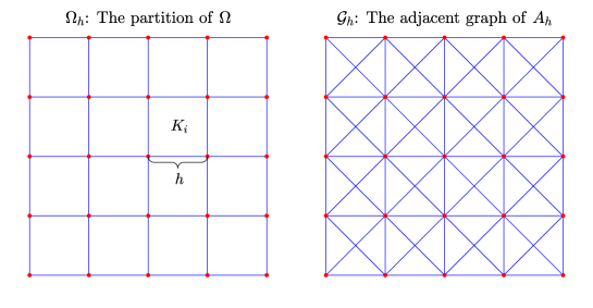
Figure 1: Illustrations of $\Omega_{h}$ and $\mathcal{G}_{h}$.

Let $\Omega_{h}=\mathop{\cup}_{i}K_{i}$ be a subdivision of $\Omega$, where each $K_{i}$ is a square with edge length $h=2^{-k},\,k\in\mathbb{N}$. The stiffness matrix $A_{h}\in\,{\mathbb{R}}^{N_{h}\times N_{h}}$ corresponds to $\Omega_{h}$ is sparse and symmetric positive semidefinite with $N_{h}=(1+1/h)^{2}$. Moreover, $A_{h}$ is the Laplacian matrix of some connected graph $\mathcal{G}_{h}$, which can be obtained from $\Omega_{h}$ by adding the two diagonal lines of each element $K_{i}$; see Fig. 1.

We apply AMG $W$-cycle iteration 42 and PCG (cf. [78, Algorithm 9.1]) to 57 with different $\epsilon$ and mesh size $h$. For PCG, we choose the diagonal (Jacobi) preconditioner. For AMG, we adopt weighted Jacobi smoother $R_{\ell}=1/2D_{\ell}$ and the number of smoothing iteration is $\theta=5$. Additionally, to obtain a maximal independent set via Algorithm 5 and avoid the for loop, we adopt a subroutine from the MATLAB software package: $i$FEM [21].

Table 1: Number of iterations of AMG and PCG.

$1/h$	$\epsilon=10^{-4}$		$\epsilon=10^{-6}$		$\epsilon=10^{-8}$		$\epsilon=10^{-10}$		$\epsilon=0$
	$\mathtt{itamg}$	$\mathtt{itpcg}$	$\mathtt{itamg}$	$\mathtt{itpcg}$	$\mathtt{itamg}$	$\mathtt{itpcg}$	$\mathtt{itamg}$	$\mathtt{itpcg}$	$\mathtt{itamg}$	$\mathtt{itpcg}$
$2^{4}$	9	62	10	66	9	69	9	52	10	52
$2^{6}$	9	230	9	250	9	266	9	201	10	201
$2^{8}$	9	789	9	906	9	969	10	740	9	740
$2^{10}$	9	1427	10	3158	9	3531	10	2680	9	2680

In Table 1, we report the number of iterations of AMG (cf. $\mathtt{itamg}$) and PCG (cf. $\mathtt{itpcg}$), under the stop criterion

$$\frac{\left\lVert{Ax_{k}-f}\right\rVert}{\left\lVert{Ax_{0}-f}\right\rVert}\leqslant\mathtt{Tol}=10^{-11}.$$

As we can see, AMG is very robust with respect to both the singular parameter $\epsilon$ and the problem size $N_{h}$. While the number of PCG iterations grows in terms of $N_{h}$. If $\epsilon$ is decreasing and larger than $\mathtt{Tol}$, then due to the nearly singular issue, $\mathtt{itpcg}$ also increases. When $\epsilon$ is close to (or is smaller than) $\mathtt{Tol}$, the term $\epsilon I$ in $A$ is negligible and 57 can be viewed almost as a singular system. In this situation, $\mathtt{itpcg}$ tends to the case $\epsilon=0$. To further show this dependence on $\epsilon$ more clearly, in Fig. 2, we plot the number of iterations for two cases: $h=2^{-7}$ and $h=2^{-9}$.

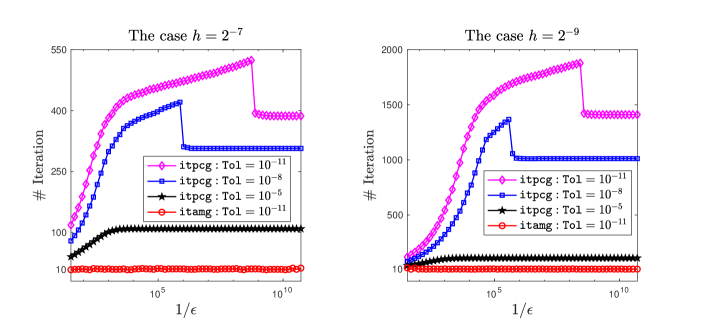
Figure 2: Growth behaviors of $\mathtt{itamg}$ and $\mathtt{itpcg}$ with respect to the parameter $\epsilon$ and the tolerance $\mathtt{Tol}$.

Table 2: The number of levels and the operator complexity of AMG.

$1/h$	$\epsilon=10^{-4}$		$\epsilon=10^{-6}$		$\epsilon=10^{-8}$		$\epsilon=10^{-10}$		$\epsilon=0$
	$J$	$\mathtt{opcom}$	$J$	$\mathtt{opcom}$	$J$	$\mathtt{opcom}$	$J$	$\mathtt{opcom}$	$J$	$\mathtt{opcom}$
$2^{4}$	4	1.47	4	1.49	4	1.41	4	1.50	4	1.40
$2^{6}$	5	1.64	5	1.62	5	1.65	5	1.62	5	1.65
$2^{8}$	6	1.66	6	1.68	6	1.67	6	1.67	6	1.66
$2^{10}$	7	1.68	7	1.69	7	1.68	7	1.69	7	1.69

Except for the number of iterations, we also record two crucial ingredients of the multilevel hierarchy: (i) the number of levels $J$ and (ii) the operator complexity ($\mathtt{opcom}$ for short)

$$\mathtt{opcom}:=\frac{\sum_{\ell=1}^{J}\mathtt{nnz}(A_{\ell})}{\mathtt{nnz}(A)}.$$

The quantity $\mathtt{opcom}$ is often used to measure the computational complexity of the AMG algorithm. From Table 2, we might observe the growth magnitude $\mathcal{O}(|\ln h|)$, as mentioned in Remark 6. This is almost negligible and thus both $J$ and $\mathtt{opcom}$ are robust with respect to $h$ and $\epsilon$.

7.2 The overall IPD-SsN-AMG method

Combining Algorithms 1, 2, 3 and 4, we obtain the overall semismooth Newton-AMG-based Inexact Primal-Dual (IPD-SsN-AMG for short) method for solving the generalized transport problem 7; see Algorithm 6.

Algorithm 6 The overall IPD-SsN-AMG method

0:  KKT tolerance: $\mathtt{KKT\_Tol}$.   SsN iteration tolerance: $\mathtt{SsN\_Tol}$.   Maximal SsN iteration number: $j_{\max}\in\mathbb{N}$.   Line search parameters: $\tau\in(0,1/2),\,\delta\in(0,1)$.   Initial guesses: $\beta_{0}>0,\,\lambda_{0}\in\,{\mathbb{R}}^{m+n+r}$ and $\bm{u}_{0}=\bm{v}_{0}\in\,{\mathbb{R}}^{mn+n+m}$.

1:  for $k=0,1,\cdots$ do

2:     Choose the step size $\alpha_{k}>0$.

3:     Set $\tau_{k}={}\beta_{k}(1+\alpha_{k})/\alpha_{k}^{2}$ and $\eta_{k}=\sigma+\tau_{k}$.

4:     Set $D_{k}={\rm diag}(\eta_{k}I_{mn},\tau_{k}I_{n},\tau_{k}I_{m})$ and $\bm{w}_{k}={}\widetilde{c}+\beta_{k}(\bm{u}_{k}+\alpha_{k}\bm{v}_{k})/\alpha_{k}^{2}$.

5:     Update $\displaystyle\beta_{k+1}=\beta_{k}/(1+\alpha_{k})$ and set $\widetilde{\lambda}_{k}={}\beta_{k+1}\left[\lambda_{k}-\beta_{k}^{-1}(H\bm{u}_{k}-b)\right]-b$.

6:     Set $\lambda_{\rm new}=\lambda_{k}$.

7:     for $j=0,1,\cdots$ do {SsN iteration}

8:        Set $\lambda_{\rm old}=\lambda_{\rm new}$ and $\bm{z}_{k}=D^{-1}_{k}(\bm{w}_{k}-H^{\top}\lambda_{\rm new})$.

9:        Compute the diagonal matrix $U_{k}\in\partial{\rm proj}_{\Sigma}\left(\bm{z}_{k}\right)$ from 31.

10:        Transform the linear equation

$$\mathcal{J}_{k}\zeta=\left(\beta_{k+1}I+HD_{k}^{-1}U_{k}H^{\top}\right)\zeta=-F_{k}(\lambda_{\rm old})$$

into the reduced graph Laplacian system 38.

11:        Apply Algorithms 3 and 4 to 38 and recover the solution $\zeta$.  {AMG}

12:        Update $\lambda_{\rm new}=\lambda_{\rm old}+\delta^{\ell}\zeta$ with the smallest nonnegative integer $\ell\in\mathbb{N}$ that satisfies $\mathcal{F}_{k}(\lambda_{\rm old}+\delta^{\ell}\zeta)\leq\mathcal{F}_{k}(\lambda_{\rm old})+\tau\delta^{\ell}\left\langle{F_{k}(\lambda_{\rm old}),\zeta}\right\rangle$.  {Line search}

13:        if $\left\lVert{F_{k}(\lambda_{\rm new})}\right\rVert\leq\mathtt{SsN\_Tol}$ or $j\geq j_{\rm max}$ then {Check the SsN iteration}

14:           break

15:        end if

16:     end for

17:     Update $\lambda_{k+1}=\lambda_{\rm new},\,\bm{u}_{k+1}={\rm proj}_{\Sigma}\left(\bm{z}_{k}\right)$ and $\bm{v}_{k+1}=\bm{u}_{k+1}+(\bm{u}_{k+1}-\bm{u}_{k})/\alpha_{k}$.

18:     if ${\rm Res}(k+1)\leqslant\mathtt{KKT\_Tol}$ then {Check the KKT residual}

19:        break

20:     end if

21:  end for

Detailed parameter choices and operations are explained in order. In step 11, the settings of the AMG $W$-cycle are the same as that in Section 7.1. Note that Algorithm 3 requires the connected components of the graph $\mathcal{G}=(\mathcal{V},\mathcal{E})$ with respect to the Laplacian matrix $\mathcal{A}_{0}$ in 38. This can be done by using graph searching algorithms [44] such as breadth first search (with the complexity $\mathcal{O}(|\mathcal{V}||\mathcal{E}|)$) and depth first search (with the complexity $\mathcal{O}(|\mathcal{E}|)=\mathcal{O}(\mathtt{nnz}(\mathcal{A}_{0}))$). Thanks to the bipartite structure, we adopt the MATLAB built-in function $\mathtt{dmperm}$ that provides the Dulmage–Mendelsohn decomposition of $\mathcal{A}_{0}$ and also returns the connected components.

For SsN iteration, the line search parameters are $\tau=0.2$ and $\delta=0.9$, and in step 13, it shall be terminated when either $j$ is larger than the maximal iteration number $j_{\rm max}=15$ or $\left\lVert{F_{k}(\lambda_{\rm new})}\right\rVert$ is smaller than the tolerance $\mathtt{SsN\_Tol}=\max\{\beta_{k}(k+1)^{-2},\,10^{-11}\}$.

Moreover, in step 18 we impose the stop criterion

(58) $${\rm Res}(k):=\max\left\{\frac{{\rm KKT}(x_{k})}{{\rm KKT}(x_{0})},\,\frac{{\rm KKT}(y_{k})}{{\rm KKT}(y_{0})},\,\frac{{\rm KKT}(z_{k})}{{\rm KKT}(z_{0})},\,\frac{{\rm KKT}(\lambda_{k})}{{\rm KKT}(\lambda_{0})}\right\}\leq\mathtt{KKT\_Tol},$$

where $\mathtt{KKT\_Tol}>0$ denotes the tolerance and the KKT residuals are defined by

$$\left\{\begin{aligned} {\rm KKT}(x_{k}):={}&\left\lVert{x_{k}-{\rm proj}_{\mathcal{X}}(\sigma\phi+(1-\sigma)x_{k}-c-G^{\top}\lambda_{k})}\right\rVert,\\ {\rm KKT}(y_{k}):={}&\left\lVert{y_{k}-{\rm proj}_{\mathcal{Y}}(y_{k}-I_{Y}^{\top}\lambda_{k})}\right\rVert,\\ {\rm KKT}(z_{k}):={}&\left\lVert{z_{k}-{\rm proj}_{\mathcal{Z}}(z_{k}-I_{Z}^{\top}\lambda_{k})}\right\rVert,\\ {\rm KKT}(\lambda_{k}):={}&\left\lVert{Gx_{k}+I_{Y}y_{k}+I_{Z}z_{k}-b}\right\rVert.\end{aligned}\right.$$

In the sequel, we investigate the performance of our IPD-SsN-AMG method on specific problems including optimal transport, Birkhoff projection and partial optimal transport. Also, comparisons with the semismooth Newton-based augmented Lagrangian methods proposed in [55, 56] and the accelerated ADMM method in [64] will be presented, under the same stopping condition 58 with $\mathtt{KKT\_Tol}=10^{-6}$.

The methods in [55, 56] adopt PCG as the linear system solver, and the (super-)linear convergence analysis is based on classical proximal point framework together with proper error bound assumption. For convenience, we abbreviate these two methods simply as ALM-SsN-PCG. The method in [64], denoted shortly by Acc-ADMM, possesses sublinear rates $\mathcal{O}(1/k)$ and $\mathcal{O}(1/k^{2})$ respectively for convex and partially strongly convex objectives.

We note that, as summarized in the introduction part, some other optimization solvers, such as entropy regularization methods and interior-point methods, can also be applied to transport-like problems considered here. However, entropy-based methods provide approximate solutions only with a fixed tolerance, which is almost the same magnitude as the regularization parameter. Interior-point methods utilize the barrier function and require linear system solver as well. Hence, it would be interesting to studying the efficiency comparison between PCG and AMG, and we leave this as our future topic.

7.2.1 Optimal transport

Let us focus on the optimal mass transport 2 with $m=n\in\mathbb{N}$. The mass distributions $\mu,\,\nu\in\,{\mathbb{R}}^{n}_{+}$ are generated randomly, and we consider two kinds of cost matrices:

• Random cost:

  (59) $$C=\left(C_{ij}\right)_{n\times n}\quad\text{with}\quad C_{ij}\sim\mathcal{U}([0,1]),$$

  where $\mathcal{U}([0,1])$ denotes the uniform distribution on $[0,1]$;

• Quadratic distance cost:

  (60) $$C=\left(C_{ij}\right)_{n\times n}\quad\text{with}\quad C_{ij}=\left\lVert{x_{i}-x_{j}}\right\rVert^{2},$$

  where $\{x_{i}\}_{i=1}^{n}$ are the grid points in the uniform subdivision of $\Omega=(0,1)^{2}$ with mesh size $1/h=\sqrt{n}-1$; see Fig. 1.

As discussed in Remark 3, our IPD-SsN-AMG converges at least linearly as long as the step size is bounded below $\alpha_{k}\geq\alpha_{0}>0$. Practically, we are not allowed to increase $\alpha_{k}$ as large as we can. Hence, we choose $\alpha_{k}\geq 1$ for small $k(\leq 10)$ and set $\alpha_{k}\in(0,1)$ for large $k$. For ALM-SsN-PCG, there are two crucial parameters $\sigma_{k}$ and $\tau_{k}$; see equation (18) in [55, Algorithm 1]. Theoretically, letting $\sigma_{k}$ increase to $\infty$ and $\tau_{k}$ decrease to $\tau_{\infty}>0$ implies superlinear convergence. However, for the sake of practical computation, we set the moderate choice: $\sigma_{k}=\mathcal{O}(k^{2})$ and $\tau_{k}=\mathcal{O}(1/k)$. Additionally, we provide a warming-up initial guess for both two algorithms by running Acc-ADMM 100 times.

	IPD-SsN-AMG				ALM-SsN-PCG				Acc-ADMM
$m=n$	$\mathtt{itIPD}$	$\mathtt{itSsN}$	$\mathtt{itamg}$		$\mathtt{itALM}$	$\mathtt{itssn}$	$\mathtt{itpcg}$		it	residual
			max	aver			max	aver
$1000$	19	170	13	7	46	286	731	190	5000	6.42e-02
$2000$	29	233	14	7	54	416	1299	235	5000	1.05e-01
$3000$	29	279	15	7	57	463	2059	284	5000	3.18e-01
$4000$	39	311	13	6	61	531	2100	264	5000	4.95e-01

Table 3: Numerical results for optimal transport with random cost 59.

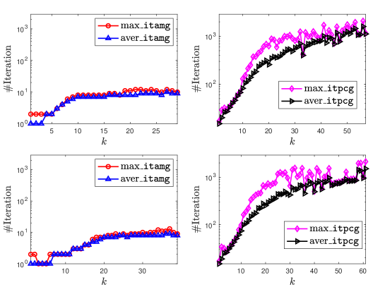
Figure 3: Growth behaviors of $\mathtt{itamg}$ and $\mathtt{itpcg}$ for optimal transport with random cost: $m=n=3000$ for top row and $m=n=4000$ for bottom row.

Numerical results with random cost 59 and quadratic distance cost 60 are listed in Table 3 and Table 4, respectively. We record (i) the number of iterations ($\mathtt{itIPD}$ and $\mathtt{itALM}$), (ii) the total number of SsN iterations ($\mathtt{itSsN}$ and $\mathtt{itssn}$), and (iii) the maximum (max) and average (aver) iteration number of AMG ($\mathtt{itamg}$) and PCG ($\mathtt{itpcg}$). Besides, Acc-ADMM is stopped at $k=5000$ and we report the corresponding relative KKT residuals.

We find that $\mathtt{itIPD}$ ($\mathtt{itSsN}$) is better than $\mathtt{itALM}$ ($\mathtt{itssn}$) for random cost but slightly inferior for quadratic distance cost. Particularly, $\mathtt{itamg}$ is more robust than $\mathtt{itpcg}$, and we also plot the growth behaviors in Figs. 3 and 4. As we can see, $\mathtt{itamg}$ stays around 10 while $\mathtt{itpcg}$ increases dramatically as $k$ does.

	IPD-SsN-AMG				ALM-SsN-PCG				Acc-ADMM
$m=n$	$\mathtt{itIPD}$	$\mathtt{itSsN}$	$\mathtt{itamg}$		$\mathtt{itALM}$	$\mathtt{itssn}$	$\mathtt{itpcg}$		it	residual
			max	aver			max	aver
$900$	29	215	11	7	20	183	628	163	5000	1.03e-01
$1600$	29	225	11	7	21	226	979	191	5000	1.69e-01
$2500$	43	328	12	7	25	277	1556	278	5000	2.51e-01
$3600$	40	352	13	7	35	360	1798	640	5000	3.48e-01

Table 4: Numerical results for optimal transport with quadratic distance cost 60.

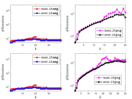
Figure 4: Growth behaviors of $\mathtt{itamg}$ and $\mathtt{itpcg}$ for optimal transport with quadratic distance cost: $m=n=2500$ for top row and $m=n=3600$ for bottom row.

	IPD-SsN-AMG				ALM-SsN-PCG				Acc-ADMM
$m=n$	$\mathtt{itIPD}$	$\mathtt{itSsN}$	$\mathtt{itamg}$		$\mathtt{itALM}$	$\mathtt{itssn}$	$\mathtt{itpcg}$		it	residual
			max	aver			max	aver
$2000$	6	18	1	1	8	25	15	10	5000	3.33e-03
$3000$	6	17	1	1	7	24	14	10	5000	3.32e-03
$4000$	6	19	1	1	7	24	20	10	5000	3.23e-03
$5000$	6	19	1	1	7	24	26	10	5000	3.20e-03

Table 5: Numerical outputs for Birkhoff projection without entry constraint.

7.2.2 Birkhoff projection

We then move to the Birkhoff projection 3 with possible entry constraint 4. For this problem, we choose fixed large step size $\alpha_{k}=10$ for our IPD-SsN-AMG. Numerical outputs with random data are presented in Tables 5 and 6. Notice that both two algorithms work well, and $\mathtt{itamg}$ is still superior than $\mathtt{itpcg}$ (which is also quite robust). This might be due to the strongly convex property of the problem itself.

	IPD-SsN-AMG				ALM-SsN-PCG				Acc-ADMM
$m=n$	$\mathtt{itIPD}$	$\mathtt{itSsN}$	$\mathtt{itamg}$		$\mathtt{itALM}$	$\mathtt{itssn}$	$\mathtt{itpcg}$		it	residual
			max	aver			max	aver
$1000$	6	13	1	1	7	21	15	11	5000	3.81e-03
$2000$	6	20	1	1	8	24	15	10	5000	3.42e-03
$3000$	6	18	1	1	6	30	14	11	5000	3.30e-03
$4000$	6	17	1	1	5	42	20	12	5000	3.22e-03

Table 6: Numerical outputs for Birkhoff projection with entry constraint.

7.2.3 Partial optimal transport

Finally, let us consider the problem of partial optimal transport 5 with random cost 59 and quadratic distance cost 60. Again, the marginal distributions $\mu$ and $\nu$ and the fraction of mass $a$ are generated randomly.

From Tables 7 and 8, we observe that: (i) similar with the results of optimal transport (see Tables 3 and 4), $\mathtt{itIPD}$ is much less than $\mathtt{itALM}$ for random cost but slightly more than that for quadratic distance cost; (ii) $\mathtt{itSsN}$ is better than $\mathtt{itssn}$ for both two cases; (iii) $\mathtt{itamg}$ stays robust and outperforms $\mathtt{itpcg}$.

Growth behaviors of $\mathtt{itamg}$ and $\mathtt{itpcg}$ are displayed in Figs. 5 and 6. We find that $\mathtt{itamg}$ is temperately increasing within few initial steps while $\mathtt{itpcg}$ is not robust with respect to both the iteration process (i.e., the number $k$) and the problem size.

	IPD-SsN-AMG				ALM-SsN-PCG				Acc-ADMM
$m=n$	$\mathtt{itIPD}$	$\mathtt{itSsN}$	$\mathtt{itamg}$		$\mathtt{itALM}$	$\mathtt{itssn}$	$\mathtt{itpcg}$		it	residual
			max	aver			max	aver
$1000$	20	152	35	14	66	274	452	154	5000	1.55e-01
$2000$	34	205	25	8	72	352	644	145	5000	4.12e-01
$3000$	34	225	23	6	74	411	426	87	5000	8.71e-01
$4000$	33	238	29	6	81	462	555	100	5000	3.22e+01

Table 7: Numerical results for partial optimal transport with random cost 59.

	IPD-SsN-AMG				ALM-SsN-PCG				Acc-ADMM
$m=n$	$\mathtt{itIPD}$	$\mathtt{itSsN}$	$\mathtt{itamg}$		$\mathtt{itALM}$	$\mathtt{itssn}$	$\mathtt{itpcg}$		it	residual
			max	aver			max	aver
$900$	31	154	19	5	18	139	95	60	5000	5.95e-01
$1600$	32	155	28	5	22	176	98	63	5000	1.77e-01
$2500$	32	196	36	6	25	223	128	64	5000	6.20e-01
$3600$	31	204	46	7	29	244	138	66	5000	5.60e-01

Table 8: Numerical results for partial optimal transport with quadratic distance cost 60.

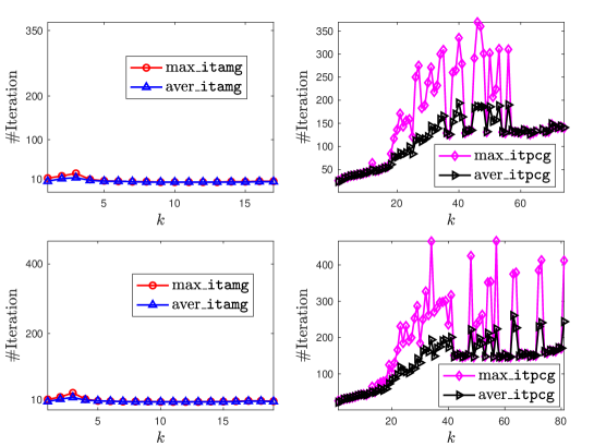
Figure 5: Growth behaviors of $\mathtt{itamg}$ and $\mathtt{itpcg}$ for partial optimal transport with random cost: $m=n=3000$ for top row and $m=n=4000$ for bottom row.

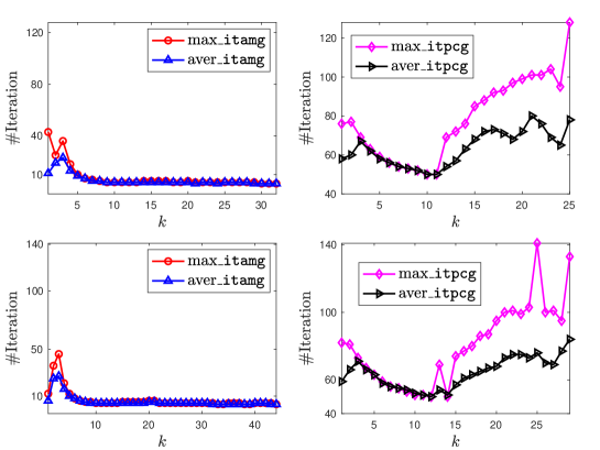
Figure 6: Growth behaviors of $\mathtt{itamg}$ and $\mathtt{itpcg}$ for partial optimal transport with quadratic distance cost: $m=n=2500$ for top row and $m=n=3600$ for bottom row.

8 Conclusion

In this paper, we propose an efficient semismooth Newton-AMG-based inexact primal-dual method for a large class of transport-like problems that share the common feature of marginal distribution constraint. We follow the differential equation solver approach and prove the (super-)linear convergence rate via discrete Lyapunov function. Utilizing the hidden graph structure of the linear system arising from the semismooth Newton iteration, we use the algebraic multilevel method and establish a robust estimate of the two-level case by the Xu-Zikatanov identity. Extensive numerical experiments are also provided to validate the performance of our algorithm.

References

- [1] B. K. Ahuja. Network Flows: Theory, Algorithms, and Applications. Prentice Hall, 1993.
- [2] J. Altschuler, J. Niles-Weed, and P. Rigollet. Near-linear time approximation algorithms for optimal transport via Sinkhorn iteration. In 31st Conference on Neural Information Processing Systems (NIPS 2017), Long Beach, CA, USA, 2017.
- [3] M. Arjovsky, S. Chintala, and L. Bottou. Wasserstein generative adversarial networks. In Proceedings of the 34 th International Conference on Machine Learning, volume 70, Sydney, Australia, 2017. PMLR.
- [4] Z. Bai, D. Chu, and R. C. E. Tan. Computing the nearest doubly stochastic matrix with a prescribed entry. SIAM J. Sci. Comput., 29(2):635–655, 2007.
- [5] Z. Bai and R. Freund. A partial pade-via-Lanczos method for reduced-order modeling. Linear Algebra Appl., 332:139–164, 2001.
- [6] H. Bauschke and P. Combettes. Convex Analysis and Monotone Operator Theory in Hilbert Spaces. CMS Books in Mathematics. Springer Science+Business Media, New York, 2011.
- [7] J.-D. Benamou. Optimal transportation, modelling and numerical simulation. Acta Numer., 30:249–325, 2021.
- [8] J.-D. Benamou, G. Carlier, M. Cuturi, L. Nenna, and G. Peyré. Iterative Bregman projections for regularized transportation problems. SIAM J. Sci. Comput., 37(2):A1111–A1138, 2015.
- [9] D. P. Bertsekas. Auction algorithms for network flow problems: a tutorial introduction. Comput. Optim. Appl., 1(1):7–66, 1992.
- [10] D. Bertsimas and J. Tsitsiklis. Introduction to Linear Optimization. Athena Scientific, 1997.
- [11] R. Blaheta. Algebraic Multilevel Methods with Aggregations: An Overview. In Large-Scale Scientific Computing, volume 3743, pages 3–14. Springer Berlin Heidelberg, Berlin, 2006.
- [12] J. H. Bramble, J. E. Pasciak, and J. Xu. Parallel multilevel preconditioners. Math. Comput., 55(191):1–22, 1990.
- [13] C. Brauer, C. Clason, D. Lorenz, and B. Wirth. A Sinkhorn-Newton method for entropic optimal transport. arXiv:1710.06635, 2018.
- [14] S. C. Brenner and L. R. Scott. The Mathematical Theory of Finite Element Methods. Number 15 in Texts in Applied Mathematics. Springer, New York, NY, 3rd edition, 2008.
- [15] H. Brezis. Remarks on the Monge–Kantorovich problem in the discrete setting. Comptes Rendus Mathematique, 356(2):207–213, 2018.
- [16] W. L. Briggs, V. E. Henson, and S. F. McCormick. A Multigrid Tutorial. Society for Industrial and Applied Mathematics, USA, 2nd edition, 2000.
- [17] R. Brualdi. Combinatorial Matrix Classes. Cambridge University Press, New York, 2006.
- [18] R. E. Burkard, M. Dell’Amico, and S. Martello. Assignment Problems. SIAM, Society for Industrial and Applied Mathematics, Philadelphia, 2009.
- [19] L. Caffarelli and R. McCann. Free boundaries in optimal transport and Monge-Ampère obstacle problems. Ann. Math., 171(2):673–730, 2010.
- [20] L. Chapel and M. Z. Alaya. Partial optimal transport with applications on positive-unlabeled learning. In 34th Conference on Neural Information Processing Systems (NeurIPS 2020), Vancouver, Canada, 2020.
- [21] L. Chen. FEM: an integrated finite element methods package in MATLAB. Technical report, 2009.
- [22] L. Chen. Deriving the X-Z identity from auxiliary space method. In Y. Huang, R. Kornhuber, O. Widlund, and J. Xu, editors, Domain Decomposition Methods in Science and Engineering XIX, volume 78, pages 309–316. Springer, Berlin, 2011.
- [23] L. Chen, X. Hu, and S. M. Wise. Convergence analysis of the fast subspace descent methods for convex optimization problems. Math. Comput., 89(325):2249–2282, 2020.
- [24] L. Chen, R. H. Nochetto, and J. Xu. Optimal multilevel methods for graded bisection grids. Numer. Math., 120:1–34, 2012.
- [25] A. Chernov, P. Dvurechensky, and A. Gasnikov. Fast primal-dual gradient method for strongly convex minimization problems with linear constraints. In Y. Kochetov, M. Khachay, V. Beresnev, E. Nurminski, and P. Pardalos, editors, 9th Discrete Optimization and Operations Research, volume 9869 of Lecture Notes in Computer Science, pages 391–403, Vladivostok, Russia, 2016. Springer, Cham.
- [26] L. Chizat, G. Peyré, B. Schmitzer, and F.-X. Vialard. Scaling algorithms for unbalanced optimal transport problems. Math. Comput., 87(314):2563–2609, 2018.
- [27] F. H. Clarke. Optimization and Nonsmooth Analysis. Number 5 in Classics in Applied Mathematics. Society for Industrial and Applied Mathematics, 1987.
- [28] R. Cominetti and J. S. Martín. Asymptotic analysis of the exponential penalty trajectory in linear programming. Math. Program., 67(1-3):169–187, 1994.
- [29] N. Courty, R. Flamary, D. Tuia, and A. Rakotomamonjy. Optimal transport for domain adaptation. IEEE Transactions on Pattern Analysis and Machine Intelligence, 39(9):1853–1865, 2017.
- [30] M. Cuturi. Sinkhorn distances: Lightspeed computation of optimal transport. In Advances in Neural Information Processing Systems 26, pages 2292–2300, 2013.
- [31] J. E. Dennis and R. B. Schnabel. Numerical Methods for Unconstrained Optimization and Nonlinear Equations. Number 16 in Classics in applied mathematics. Society for Industrial and Applied Mathematics, Philadelphia, 1996.
- [32] P. Dvurechensky, A. Gasnikov, and A. Kroshnin. Computational optimal transport: complexity by accelerated gradient descent is better than by Sinkhorn’s algorithm. In Proceedings of the 35 th International Conference on Machine Learning, volume 80, Stockholm, Sweden, 2018. PMLR.
- [33] J. Eckstein and D. Bertsekas. An alternating direction method for linear programming. Technical report LIDS-P-1967, Cambridge, 1990.
- [34] F. Facchinei and J. Pang. Finite-Dimensional Variational Inequalities and Complementarity Problems, vol 2. Springer, New York, 2003.
- [35] A. R. Ferguson and G. B. Dantzig. The allocation of aircraft to routes–An example of linear programming under uncertain demand. Management Science, 3(1), 1956.
- [36] A. Figalli. The optimal partial transport problem. Arch. Ration. Mech. Anal., 195(2):533–560, 2010.
- [37] F. Fogel, R. Jenatton, F. Bach, and A. d’Aspremont. Convex relaxations for permutation problems. In Advances in Neural Information Processing Systems 26, pages 1016–1024, 2013.
- [38] A. V. Gasnikov, E. B. Gasnikova, Y. E. Nesterov, and A. V. Chernov. Efficient numerical methods for entropy-linear programming problems. Comput. Math. Math. Phys., 56(4):514–524, 2016.
- [39] W. Glunt, T. L. Hayden, and R. Reams. The nearest “doubly stochastic” matrix to a real matrix with the same first moment. Numer. Linear Algebr. Appl., 5(6):475–482, 1998.
- [40] S. Guminov, P. Dvurechensky, N. Tupitsa, and A. Gasnikov. Accelerated alternating minimization, accelerated Sinkhorn’s algorithm and accelerated iterative Bregman projections. arXiv:1906.03622, 2021.
- [41] W. Hackbusch. Multi-Grid Methods and Applications. Springer, Berlin, 2011.
- [42] R. Hug, E. Maitre, and N. Papadakis. Multi-physics optimal transportation and image interpolation. ESAIM: Math. Model. Numer. Anal., 49(6):1671–1692, 2015.
- [43] B. Jiang, Y.-F. Liu, and Z. Wen. -norm regularization algorithms for optimization over permutation matrices. SIAM J. Optim., 26(4):2284–2313, 2016.
- [44] D. Jungnickel. Graphs, Networks, and Algorithms. Number 5 in Algorithms and Computation in Mathematics. Springer, Berlin, 2nd edition, 2005.
- [45] K. Kandasamy, W. Neiswanger, J. Schneider, B. Poczos, and E. Xing. Neural architecture search with Bayesian optimisation and optimal transport. In Advances in Neural Information Processing Systems 31, 2018.
- [46] L. Kantorovich. On the translocation of masses. Dokl. Akad. Nauk. USSR (N.S.), 37:199–201, 1942.
- [47] R. N. Khoury. Closest matrices in the space of generalized doubly stochastic matrices. J. Math. Anal. Appl., 222(2):562–568, 1998.
- [48] J. Korman and R. J. McCann. Optimal transportation with capacity constraints. Trans. Am. Math. Soc., 367(3):1501–1521, 2014.
- [49] Y.-J. Lee, J. Wu, J. Xu, and L. Zikatanov. Robust subspace correction methods for nearly singular systems. Math. Models Meth. Appl. Sci., 17(11):1937–1963, 2007.
- [50] Y. T. Lee and A. Sidford. Path finding methods for linear programming: Solving linear programs in iterations and faster algorithms for maximum flow. In 2014 IEEE 55th Annual Symposium on Foundations of Computer Science, pages 424–433. IEEE, 2014.
- [51] B. Li and X. Xie. A two-level algorithm for the weak Galerkin discretization of diffusion problems. J. Comput. Appl. Math., 287:179–195, 2015.
- [52] B. Li and X. Xie. BPX preconditioner for nonstandard finite element methods for diffusion problems. SIAM J. Numer. Anal., 54(2):1147–1168, 2016.
- [53] B. Li, X. Xie, and S. Zhang. Analysis of a two-level algorithm for HDG methods for diffusion problems. Commun. Comput. Phys., 19(5):1435–1460, 2016.
- [54] H. Li and Z. Lin. Accelerated alternating direction method of multipliers: An optimal nonergodic analysis. J. Sci. Comput., 79(2):671–699, 2019.
- [55] X. Li, D. Sun, and K.-C. Toh. An asymptotically superlinearly convergent semismooth Newton augmented Lagrangian method for Linear Programming. SIAM J. Optim., 30(3):2410–2440, 2020.
- [56] X. Li, D. Sun, and K.-C. Toh. On the efficient computation of a generalized Jacobian of the projector over the Birkhoff polytope. Math. Program., 179(1-2):419–446, 2020.
- [57] Q. Liao, J. Chen, Z. Wang, B. Bai, S. Jin, and H. Wu. Fast Sinkhorn I: An algorithm for the Wasserstein-1 metric. arXiv:2202.10042, 2022.
- [58] C. H. Lim and S. J. Wright. Beyond the Birkhoff polytope: convex relaxations for vector permutation problems. In Advances in Neural Information Processing Systems, pages 2168–2176, 2014.
- [59] M. Lin, D. Sun, and K.-C. Toh. An augmented Lagrangian method with constraint generations for shape-constrained convex regression problems. Math. Program., 14:223–270, 2022.
- [60] T. Lin, N. Ho, and M. I. Jordan. On efficient optimal transport: An analysis of greedy and accelerated mirror descent algorithms. In International Conference on Machine Learning, pages 3982–3991. PMLR, 2019.
- [61] Y. Liu, Z. Wen, and W. Yin. A multiscale semi-smooth Newton method for optimal transport. J. Sci. Comput., 91(2):1–39, 2022.
- [62] H. Luo. Accelerated differential inclusion for convex optimization. Optimization, https://doi.org/10.1080/02331934.2021.2002327, 2021.
- [63] H. Luo. Accelerated primal-dual methods for linearly constrained convex optimization problems. arXiv:2109.12604, 2021.
- [64] H. Luo. A unified differential equation solver approach for separable convex optimization: splitting, acceleration and nonergodic rate. arXiv:2109.13467, 2021.
- [65] H. Luo. A primal-dual flow for affine constrained convex optimization. ESAIM: Control, Optimisation and Calculus of Variations, 28:10.1051/cocv/2022032, 2022.
- [66] B. Lévy. Partial optimal transport for a constant-volume Lagrangian mesh with free boundaries. J. Comput. Phys., 451:1–26, 2022.
- [67] J. Maas, M. Rumpf, C. Schönlieb, and S. Simon. A generalized model for optimal transport of images including dissipation and density modulation. ESAIM: Math. Model. Numer. Anal., 49(6):1745–1769, 2015.
- [68] O. L. Mangasarian and T.-H. Shiau. Lipschitz continuity of solutions of linear inequalities, programs and complementarity problems. SIAM J. Control Optim., 25(3):583–595, 1987.
- [69] Q. Mérigot and B. Thibert. Optimal Transport: Discretization and Algorithms. In Handbook of Numerical Analysis, volume 22, pages 133–212. Elsevier, 2021.
- [70] A. Padiy, O. Axelsson, and B. Polman. Generalized augmented matrix preconditioning approach and its application to iterative solution of ill-conditioned algebraic systems. SIAM J. Matrix Anal. Appl., 22(3):793–818, 2001.
- [71] V. M. Panaretos and Y. Zemel. Amplitude and phase variation of point processes. Ann. Stat., 44(2):771–812, 2016.
- [72] O. Pele and M. Werman. Fast and robust earth mover’s distances. In In 2009 IEEE 12th International Conference on Computer Vision, pages 460–467, 2009.
- [73] G. Peyré and M. Cuturi. Computational optimal transport. Found. Trends Mach. Learn., 11(5-6):1–257, 2019.
- [74] L. Qi. Convergence analysis of some algorithms for solving nonsmooth equations. Math. Oper. Res., 18(1):227–244, 1993.
- [75] L. Qi and J. Sun. A nonsmooth version of Newton’s method. Math. Program., 58(1-3):353–367, 1993.
- [76] S. Robinson. Bounds for error in the solution set of a perturbed linear program. Linear Algebra Appl., 6(C):69–81, 1973.
- [77] Y. Rubner, C. Tomasi, and L. J. Guibas. The earth mover’s distance as a metric for image retrieval. International Journal of Computer Vision, 40(2):99–121, 2000.
- [78] Y. Saad. Iterative Methods for Sparse Linear Systems. Society for Industrial and Applied Mathematics, USA, 2nd edition, 2003.
- [79] R. Sinkhorn. Diagonale quivalence to matrices with prescribed row and columnsums. The American Mathematical Monthly, 74(4):402–405, 1967.
- [80] G. Székely and M. Rizzo. Testing for equal distributions in high dimension. In Inter-Stat (London), pages 1–16, 2004.
- [81] U. Trottenberg, C. W. Oosterlee, and A. Schüller. Multigrid. Academic Press, San Diego, 2001.
- [82] C. Villani. Topics in Optimal Transportation. American Mathematical Society, 2003.
- [83] C. Villani. Optimal Transport: Old and New. Number 338 in Grundlehren der mathematischen Wissenschaften. Springer, Berlin, 2009.
- [84] Y. Wu, L. Chen, X. Xie, and J. Xu. Convergence analysis of V-Cycle multigrid methods for anisotropic elliptic equations. IMA J. Numer. Anal., 32(4):1329–1347, 2012.
- [85] J. Xu. Theory of Multilevel Methods. PhD Thesis, Cornell University, Ithaca, New York, 1989.
- [86] J. Xu. A new class of iterative methods for nonself-adjoint or indefinite problems. SIAM J. Numer. Anal., 29(2):303–319, 1992.
- [87] J. Xu. Two-grid discretization techniques for linear and nonlinear PDEs. SIAM J. Numer. Anal., 33(5):1759–1777, 1996.
- [88] J. Xu. Multilevel Iterative Methods. Lecture Notes. Penn State University, 2017.
- [89] J. Xu and L. Zikatanov. The method of alternating projections and the method of subspace corrections in Hilbert space. J. Am. Math. Soc., 15(3):573–597, 2002.
- [90] J. Xu and L. Zikatanov. Algebraic multigrid methods. Acta Numer., 26:591–721, 2017.
- [91] Y. Xu. Accelerated first-order primal-dual proximal methods for linearly constrained composite convex programming. SIAM J. Optim., 27(3):1459–1484, 2017.
- [92] L. Zikatanov. Two-sided bounds on the convergence rate of two-level methods. Numer. Linear Algebr. Appl., 15(5):439–454, 2008.