Laplacian-based Cluster-Contractive t-SNE for High Dimensional Data Visualization

Abstract.

Dimensionality reduction techniques aim at representing high-dimensional data in low-dimensional spaces to extract hidden and useful information or facilitate visual understanding and interpretation of the data. However, few of them take into consideration the potential cluster information contained implicitly in the high-dimensional data. In this paper, we propose LaptSNE, a new graph-layout nonlinear dimensionality reduction method based on t-SNE, one of the best techniques for visualizing high-dimensional data as 2D scatter plots. Specifically, LaptSNE leverages the eigenvalue information of the graph Laplacian to shrink the potential clusters in the low-dimensional embedding when learning to preserve the local and global structure from high-dimensional space to low-dimensional space. It is nontrivial to solve the proposed model because the eigenvalues of normalized symmetric Laplacian are functions of the decision variable. We provide a majorization-minimization algorithm with convergence guarantee to solve the optimization problem of LaptSNE and show how to calculate the gradient analytically, which may be of broad interest when considering optimization with Laplacian-composited objective. We evaluate our method by a formal comparison with state-of-the-art methods on seven benchmark datasets, both visually and via established quantitative measurements. The results demonstrate the superiority of our method over baselines such as t-SNE and UMAP. We also provide out-of-sample extension, large-scale extension and mini-batch extension for our LaptSNE to facilitate dimensionality reduction in various scenarios.

1. Introduction

Nowadays, data in science and engineering are usually high-dimensional. For instance, the number of genes (as features) in a gene dataset is often larger than ten thousands. In computer vision, the dimension of a vectorized high-resolution image can be higher than one million. In addition, the structures of these high-dimensional data are often complicated, especially when the numbers of samples are large. Therefore, extracting potentially useful and understandable patterns from these intricate datasets becomes necessary and helpful. Among all the extant methods, dimensionality reduction (DR) is critically important for understanding the structures of large datasets. DR aims to extract or produce informative low-dimensional features from high-dimensional data. Such features can be easily visualized to identify the hidden patterns of the original data, provided that the reduced dimension is low enough, e.g. 3-D or 2-D. The low-dimensional features provide convenience for downstream tasks such as classification and clustering without the curse of dimensionality and often improve the corresponding performances.

DR has been an active and important research topic for more than fifty years. DR methods can be organized into two categories: linear methods and nonlinear methods. Principal Component Analysis (PCA) (Pearson, 1901; Jolliffe and Cadima, 2016), Multidimensional Scaling (MDS) (Sammon, 1969), and Linear Discriminant Analysis (LDA) (Fisher, 1936) are well-known linear DR methods. These methods are simple, effective, and well-understood, though they have difficulty in handling data with nonlinear low-dimensional latent structures. In the past decades, many nonlinear dimensionality reduction (NLDR) methods have been proposed to extract low-dimensional nonlinear features or visualize high-dimensional data in 2D or 3D spaces. Well-known NLDR methods include Self-Organized Map (SOM) (Kohonen, 1982), Kernel PCA (KPCA) (Schölkopf et al., 1998), Principal Curves (Hastie and Stuetzle, 1989), Locally Linear Embedding (LLE)(Roweis and Saul, 2000), Isomap (Tenenbaum et al., 2000), Laplacian Eigenmap (LE) (Baker, 1977), AutoEncoder (DeMers and Cottrell, 1992; Hinton and Salakhutdinov, 2006), t-distributed Stochastic Neighbor Embedding (t-SNE) (Van der Maaten and Hinton, 2008), and Uniform Manifold Approximation and Projection (UMAP) (McInnes et al., 2018a). Note that LLE, Isomap, and LE are not roubust to noise and outliers and their performance on real data are not satisfactory enough. KPCA, AutoEncoder, and stacked AutoEncoders are actually nonlinear feature extraction methods and are not effective in data visualization.

Among the aforementioned NLDR methods, t-SNE developed by van der Maaten and Hinton (Van der Maaten and Hinton, 2008) is arguably one of the most powerful and state-of-the-art methods in a wide range of applications. t-SNE maps the data points to a two- or three dimensional space, which exhibits the intrinsic data distribution of the original high-dimensional data. Therefore, the low-dimensional embedding always reveal trends, patterns and outliers. In many practices of scientific research, t-SNE has become an extraordinary tool of data visualization. It is worth mentioning that there have been a few variants of t-SNE (Yang et al., 2009; Carreira-Perpinán, 2010; Xie et al., 2011; Van Der Maaten, 2014; Gisbrecht et al., 2015; Pezzotti et al., 2016; Linderman et al., 2019; Chatzimparmpas et al., 2020). For instance, Yang et al. (Yang et al., 2009) generalized t-SNE to accommodate various heavy-tailed embedding similarity functions and presented a fixed-point optimization algorithm that can be applied to all heavy-tailed functions. Van Der Maaten (Van Der Maaten, 2014) proposed to use tree-based algorithms to accelerate t-SNE.

Data visualization is growing critically important nowadays for understanding the structure-complicated high-dimensional datasets, and has been recognized as one of the building blocks of data science (Donoho, 2017). In most data visualization tasks, we are interested in discovering the potential clusters of the data and indeed, the data often contain multiple clusters naturally. On such data, the outline of clusters generated by t-SNE are often overLapped and obscure, because t-SNE does not explicitly explore and exploit the potential cluster structure of the data. To tackle with this problem, in this paper, we propose a new method, LaptSNE, to construct low-dimensional embedding in a cluster-informative manner. Our contributions are three-fold.

• We present a new NLDR algorithm LaptSNE that explores and exploits the potential clusters of the data and produces cluster-informative low-dimensional visualization.

• The objective function of the proposed method involves the eigenvalues of a graph Laplacian computed from the decision variables, which leads to difficulty in solving the optimization problem. We therefore develop an effective algorithm with convergence guarantee to solve the optimization of LaptSNE.

• We provide out-of-sample extension, large-scale extension, and mini-batch extension for our LaptSNE, which facilitate the implementation of LaptSNE in various scenarios.

Experiments on many benchmark datasets (e.g. COIL20 (Nene et al., 1996a) and MNIST (Deng, 2012)) further verify the effectiveness and superiority of our methods. For instance, compared to the vanilla t-SNE, in our method, the boundaries of clusters in the 2D embedding are clearer and the clusters are more compact. Quantitative evaluations such as the k-NN generalization error and clustering NMI also confirm the superiority of our methods.

2. Preliminary Knowledge

t-SNE is actually a modification of SNE (Hinton and Roweis, 2002). They aim to preserve the pair-wise similarities from high-dimension space $\mathcal{P}$ to low-dimension $\mathcal{Q}$. Here the pair-wise similarities are quantified by neighborhood probability, i.e., the probability of two data points are neighbors mutually. Specifically, given $\left\{\mathbf{x}_{i}\right\}_{i\in[N]}\in\mathbb{R}^{D}$ (we define $[N]:=\{1,2,\ldots,N\}$ for convenience), SNE and t-SNE find a low-dimensional embedding $\left\{\mathbf{y}_{i}\right\}_{i\in[N]}\in\mathbb{R}^{d}$ where $d\ll D$, such that if $\mathbf{x}_{i}$ and $\mathbf{x}_{j}$ are close in the original data space, $\mathbf{y}_{i}$ and $\mathbf{y}_{j}$ are also close. t-SNE starts by computing the joint probability distribution over all input data, represented by a symmetric matrix $\mathbf{P_{X}}$. When $i=j$, $p_{ij}=0$. Otherwise,

$$p_{ij}=\frac{p_{i\mid j}+p_{j\mid i}}{2N},$$

where

(1) $$\quad p_{j\mid i}=\frac{\exp\left(-\left\|\mathbf{x}_{i}-\mathbf{x}_{j}\right\|_{2}^{2}/2\tau_{i}^{2}\right)}{\sum_{\ell\in[N]\backslash\{i\}}\exp\left(-\left\|\mathbf{x}_{i}-\mathbf{x}_{\ell}\right\|_{2}^{2}/2\tau_{i}^{2}\right)}.$$

Here $\tau_{i}$ denotes the bandwidth of the Gaussian kernel based on user-specified perplexity $Perp$ (Van der Maaten and Hinton, 2008). Similarly, an affinity matrix $\mathbf{Q_{Y}}$ in the low-dimensional space can be computed. Compared to SNE, t-SNE replaces the Gaussian kernel in the low dimension with T-Student kernel in one degree of freedom (same as Cauchy kernel)(Souza, 2010). The T-Student kernel can help the learning strongly repel dissimilar data points that are modeled by a small pair-wise distance in the low-dimensional representation, thus alleviating the crowding problem. Specifically, in t-SNE, for $i\neq j$,

(2) $$q_{ij}=\frac{\left(1+\left\|\mathbf{y}_{i}-\mathbf{y}_{j}\right\|_{2}^{2}\right)^{-1}}{\sum_{\ell,s\in[N],\ell\neq s}\left(1+\left\|\mathbf{y}_{\ell}-\mathbf{y}_{s}\right\|_{2}^{2}\right)^{-1}}.$$

t-SNE thus searches for $\left\{\mathbf{y}_{i}\right\}_{i\in[N]}$ to minimize the Kullback-Leibler (KL) divergence between the joint distribution of points in the input data space $\mathcal{P}$ and embedding space $\mathcal{Q}$, i.e.,

(3) $$\left(\mathbf{y}_{1},\ldots,\mathbf{y}_{N}\right) =\underset{\mathbf{y}_{1},\ldots,\mathbf{y}_{N}}{\arg\min}~{}~{}D_{KL}(\mathbf{P_{X}},\mathbf{Q_{Y}})$$

$$=\underset{\mathbf{y}_{1},\ldots,\mathbf{y}_{N}}{\arg\min}\sum_{i\neq j}q_{ij}\log\frac{p_{ij}}{q_{ij}}.$$

More details can be found in (Van der Maaten and Hinton, 2008).

3. Cluster-Contractive t-SNE

3.1. Motivation

Although t-SNE is effective in preserving local and global structures of high-dimensional data (Arora et al., 2018), it does not explore or utilize the potential cluster structures that are prevalent in real datasets (Kobak and Berens, 2019; Li et al., 2017). The potential cluster structures should be a useful prior and exploited if possible, though it is difficult to know the number of clusters of high-dimensional data in advance. If the high-dimensional data indeed consist of multiple clusters, the clusters should be preserved in the low-dimensional embedding. Thus, besides matching the similarity matrix $\mathbf{P_{X}}$ and $\mathbf{Q_{Y}}$, we also want to get a similarity graph (from the low-dimensional embedding) of which the edges between different groups have very low weights and the edges within a group have high weights. In other words, data within the same cluster are similar to each other while data in different clusters are dissimilar from each other.

However, the aforementioned objective is intractable because we do not know the clusters (or even the number of clusters) of the high-dimensional data. Note that the affinity matrix $\mathbf{P_{X}}$ in t-SNE is actually a connected graph owing to the use of Gaussian kernel. Therefore, solving (3) does guarantee preserving clusters in the low-dimension space. Even if $\mathbf{P_{X}}$ is not connected but has multiple connected components, the solution of (3) may not preserve the clusters.

To handle the problem, we consider using the graph Laplacian defined as

(4) $$\mathbf{L}=\mathbf{I}-\mathbf{D}^{-1/2}\mathbf{A}\mathbf{D}^{-1/2}.$$

It is actually a symmetric normalized Laplacian matrix. In (4), $\mathbf{A}$ ($\mathbf{Q_{Y}}$ in this paper) is an adjacency (or similarity) matrix and $\mathbf{D}$ is the degree matrix (a diagonal matrix) of $\mathbf{A}$ defined as $D_{ii}=\sum_{j}a_{ij}$. Laplacian matrix has the property of signifying the number of clusters (Proposition 1 in (Chung and Graham, 1997)), i.e., the multiplicity $k$ of the eigenvalue 0 of $\mathbf{L}$ is equal to the number of connected components $A_{1},\ldots,A_{k}$ in the graph. When the eigenvalue 0 has a multiplicity k, we can observe k completely disconnected clusters. Therefore, we propose to maximize the number of zero eigenvalues of $\mathbf{L}$ such that we may identify more clusters from the data.

3.2. Proposed Model

In order to preserve both data structure and cluster information, we may consider the following problem

(5) $$\mathop{\text{minimize}}_{\mathbf{Y}} ~{}~{}\text{KL}(\mathbf{P_{X}},\mathbf{Q_{Y}})$$

subject to $$~{}~{}\sum_{i=1}^{N}\mathbbm{1}\big{(}\sigma_{i}(\mathbf{L}_{\mathbf{Y}})=0\big{)}=k,$$

where $\mathbf{L}_{Y}$ is the symmetric normalized Laplacian matrix computed from $\mathbf{Q}_{\mathbf{Y}}$, $\sigma_{i}(\cdot)$ denotes the $i$-th eigenvalue of matrix, and $\mathbbm{1}(\cdot)$ is an indicator function with $\mathbbm{1}(\textit{True})=1$ and $\mathbbm{1}(\textit{False})=0$. In (5), we hope that there are exactly $k$ clusters in the low-dimensional embedding. But it is difficult to know $k$ in advance. We therefore relax (5) to the following regularized problem

(6) $$\mathop{\text{minimize}}_{\mathbf{Y}}\text{KL}(\mathbf{P_{X}},\mathbf{Q_{Y}})+\lambda\|\mathbf{\sigma}(\mathbf{L}_{\mathbf{Y}})\|_{0},$$

where $\boldsymbol{\sigma}(\mathbf{L}_{\mathbf{Y}})=[\sigma_{1}(\mathbf{L}_{\mathbf{Y}}),\sigma_{2}(\mathbf{L}_{\mathbf{Y}}),\ldots,\sigma_{N}(\mathbf{L}_{\mathbf{Y}})]^{\top}$ and $\lambda$ is a tuning parameter. $\|\cdot\|_{0}$ denotes the number of nonzero elements in a vector and $\|\boldsymbol{\sigma}(\mathbf{L}_{\mathbf{Y}})\|_{0}$ is actually the rank of $\mathbf{L}_{\mathbf{Y}}$. In (6), we want to increase the number of zero eigenvalues as large as possible such that the number of clusters in the data is sufficiently large. Problem (6) is NP-hard due to the presence of the $\ell_{0}$ norm. It is known that the $\ell_{p}$ (quasi) norms, $\|\mathbf{x}\|_{p}:=(\sum_{i}|x_{i}|^{p})^{1/p}$ ($0<p\leq 1$) are popular proxies of the $\ell_{0}$ norm. Particularly, $\|\mathbf{x}\|_{1}$ is a convex relaxation of $\|\mathbf{x}\|_{0}$. Therefore, we relax (6) to

(7) $$\mathop{\text{minimize}}_{\mathbf{Y}}\text{KL}(\mathbf{P_{X}},\mathbf{Q_{Y}})+\lambda\sum_{i=1}^{N}\sigma_{i}^{p}(\mathbf{L}_{\mathbf{Y}}).$$

Note that $\sum_{i=1}^{N}\sigma_{i}^{p}(\mathbf{L}_{\mathbf{Y}})\rightarrow\|\mathbf{\sigma}(\mathbf{L}_{\mathbf{Y}})\|_{0}$ when $p\rightarrow 0$. In this study, we only consider the case $p=1$ for simplicity. Then we arrive at

(8) $$\mathop{\text{minimize}}_{\mathbf{Y}}\text{KL}(\mathbf{P_{X}},\mathbf{Q_{Y}})+\lambda\mathrm{Tr}(\mathbf{V}_{\mathbf{L_{Y}}}^{\top}\mathbf{L}_{\mathbf{Y}}\mathbf{V}_{\mathbf{L_{Y}}}),$$

where $\mathbf{V}_{\mathbf{L_{Y}}}\in\mathbb{R}^{N\times N}$ denotes the eigenvectors of $\mathbf{L}_{\mathbf{Y}}$. Since $\mathbf{V}_{\mathbf{L_{Y}}}$ depends on $\mathbf{Y}$, we have to rewrite (8) as

(9) $$\mathop{\text{minimize}}_{\mathbf{Y}}\text{KL}(\mathbf{P_{X}},\mathbf{Q_{Y}})+\lambda\min_{\mathbf{V}^{\top}\mathbf{V}=\mathbf{I}}\mathrm{Tr}(\mathbf{V}^{\top}\mathbf{L}_{\mathbf{Y}}\mathbf{V}).$$

Note that in (9), the matrix multiplications in the trace operator are costly because $\mathbf{V}_{\mathbf{L_{Y}}}$ is a square matrix. On the other hand, in (8), we may just shrink the smallest few eigenvalues because in practice the number of clusters in the high-dimensional data is not large (e.g. 10 or 100) and much less than $n$. In view of the two reasons, we solve the following problem instead of (9)

(10) $$\mathop{\text{minimize}}_{\mathbf{Y}}\text{KL}(\mathbf{P_{X}},\mathbf{Q_{Y}})+\lambda\min_{\mathbf{V}_{\hat{k}}^{\top}\mathbf{V}_{\hat{k}}=\mathbf{I}}\mathrm{Tr}(\mathbf{V}_{\hat{k}}^{\top}\mathbf{L}_{\mathbf{Y}}\mathbf{V}_{\hat{k}}),$$

where $\mathbf{V}_{\hat{k}}\in\mathbb{R}^{N\times\hat{k}}$ and $\hat{k}$ is an estimated number of potential clusters in $\mathbf{X}$. This is exactly our proposed method LaptSNE.

3.3. Optimization

Note that it is non-trivial to solve (10) due to the presence of $\mathbf{V}_{\hat{k}}$. We present a majorization-minimization (Vaida, 2005) algorithm for (10). Specifically, at iteration $t$, we solve

(11) $$\mathop{\text{minimize}}_{\mathbf{Y}}\text{KL}(\mathbf{P_{X}},\mathbf{Q_{Y}})+\lambda\mathrm{Tr}(\mathbf{V}_{t-1}^{\top}\mathbf{L}_{\mathbf{Y}}\mathbf{V}_{t-1}),$$

where $\mathbf{V}_{t-1}$ is the eigenvectors of $\mathbf{L}_{\mathbf{Y}_{t-1}}$ corresponding to the smallest $\hat{k}$ eigenvalues. There is no need to obtain the exact solution of (11) and hence we propose to just update $\mathbf{Y}$ by gradient descent. For convenience, let

(12) $$\mathcal{L}_{1}(\mathbf{Y})=\text{KL}(\mathbf{P_{X}},\mathbf{Q_{Y}}),$$

(13) $${\mathcal{L}}_{2}(\mathbf{Y})=\lambda\min_{\mathbf{V}_{\hat{k}}^{\top}\mathbf{V}_{\hat{k}}=\mathbf{I}}\mathrm{Tr}(\mathbf{V}_{\hat{k}}^{\top}\mathbf{L}_{\mathbf{Y}}\mathbf{V}_{\hat{k}}),$$

(14) $$\hat{\mathcal{L}}_{2}(\mathbf{Y})=\lambda\mathrm{Tr}(\mathbf{V}_{t-1}^{\top}\mathbf{L}_{\mathbf{Y}}\mathbf{V}_{t-1}),$$

(15) $$\mathcal{L}=\mathcal{L}_{1}(\mathbf{Y})+\mathcal{L}_{2}(\mathbf{Y}),$$

(16) $$\hat{\mathcal{L}}=\mathcal{L}_{1}(\mathbf{Y})+\hat{\mathcal{L}}_{2}(\mathbf{Y}).$$

Then the one-step gradient descent is given as

(17) $$\mathbf{Y}_{t}\longleftarrow\mathbf{Y}_{t-1}-\alpha\nabla\hat{\mathcal{L}}(\mathbf{Y})$$

where $\alpha$ is the step size and $\nabla\hat{\mathcal{L}}$ denotes the derivative of $\mathcal{L}$ with respect to $\mathbf{Y}$. The procedures are summarized into Algorithm 1.

Algorithm 1 Optimization for LaptSNE

1:dataset $\mathbf{X}\in\mathbb{R}^{N\times D}$, target dimension $d$, estimate of cluster numbers $\hat{k}$, tuning parameter $\lambda$, perplexity $\delta_{\text{{Perp}}}$, step size $\alpha$, maximum iteration $T$

2:compute pairwise affinities $p_{j|i}$ with perplexity $\delta_{\text{{Perp}}}$ (refer to (Van der Maaten and Hinton, 2008))

3:set $\mathbf{P_{X}}=\left\{p_{ij}\right\}_{(i,j)\in[N]\times[N]}$ where $p_{ij}=\frac{p_{j|i}+p_{i|j}}{2N}$

4:compute the graph Laplacian $\mathbf{L}_{\mathbf{X}}$ of $\mathbf{P_{X}}$

5:Initialization: $\mathbf{Y}_{0}\longleftarrow[\mathbf{V}_{1}(\mathbf{L}_{\mathbf{X}}),\cdots,\mathbf{V}_{d}(\mathbf{L}_{\mathbf{X}})]$

6:for $t=1,2,\ldots,T$ do

7:     compute low-dimensional affinities $\{q_{ij}\}_{(i,j)\in[N]\times[N]}$

8:     compute gradient of KL divergence $\nabla\mathcal{L}_{1}(\mathbf{Y})$

9:     compute gradient of regularization $\nabla\hat{\mathcal{L}}_{2}(\mathbf{Y})$

10:     set $\mathbf{Y}_{t}\longleftarrow\mathbf{Y}_{t-1}-\alpha\left(\nabla\mathcal{L}_{1}(\mathbf{Y})+\nabla\hat{\mathcal{L}}_{2}(\mathbf{Y})\right)$

11:end for

12:cluster-contractive embedding $\mathbf{Y}_{T}\in\mathbb{R}^{N\times d}$

Proposition 0.

Suppose there exists a positive constant $L$ such that $\|\nabla\mathcal{L}(\mathbf{Y})-\nabla\mathcal{L}(\mathbf{Y}^{\prime})\|_{F}\leq L\|\mathbf{Y}-\mathbf{Y}^{\prime}\|_{F}$. Let $\mathbf{Y}_{0},\mathbf{Y}_{1},\ldots,\mathbf{Y}_{T}$ be the sequence generated by Algorithm 1 with $\alpha\leq\frac{2}{L}$. Then:
(a) $\mathcal{L}(\mathbf{Y}_{t})-\mathcal{L}(\mathbf{Y}_{t-1})\leq\frac{2-\alpha L}{2\alpha}\left\|\mathbf{Y}_{t}-\mathbf{Y}_{t-1}\right\|_{F}\leq 0$;
(b) $\mathcal{L}(\mathbf{Y}_{T})\leq\mathcal{L}(\mathbf{Y}_{0})-\frac{2-\alpha L}{2\alpha}\sum_{t=1}^{T}\left\|\mathbf{Y}_{t}-\mathbf{Y}_{t-1}\right\|_{F}$.

Proposition 1 shows that LaptSNE Algorithm 1 proves to be convergent. We defer the proof to Appendix A.1. Note that the algorithm can be accelerated by using momentum, i.e.,

$$\mathbf{Y}_{t}\longleftarrow\mathbf{Y}_{t-1}-\alpha\left(\nabla\mathcal{L}_{1}(\mathbf{Y})+\nabla\hat{\mathcal{L}}_{2}(\mathbf{Y})\right)+\beta(t)\left(\mathbf{Y}_{(t-1)}-\mathbf{Y}_{t-2}\right),$$

where $\beta(t)$ is the momentum parameter. Proving the convergence of Algorithm 1 with momentum is out of the scope of this paper and can be an future work.

3.4. Gradient of Laplacian-Composited Objective

It is non-trivial to compute the gradient of $\nabla\mathcal{L}(\mathbf{Y})$ because $\mathbf{Y}$ involves the symmetric normalized Laplacian. Here we elaborate the computation.

First, the gradient of $\mathcal{L}_{2}(\mathbf{Y})$ ($\lambda$ is omitted for convenience) with respect to $\mathbf{Y}$ can be expressed as

(18) $$\frac{\partial\mathrm{Tr}(\mathbf{V^{\top}LV})}{\partial\mathbf{Y}}=\sum_{m,n}\left(\sum_{i,j}(\mathbf{VV^{\top}})_{ij}\frac{\partial\mathbf{L}_{ij}}{\partial q_{mn}}\right)\frac{\partial q_{mn}}{\partial\mathbf{Y}}.$$

The symmetric normalized Laplacian matrix $\mathbf{L}$ is constructed via $\mathbf{Q_{Y}}$ (note that $q_{ii}=0,\forall i$), and the matrix representation of $\mathbf{L}$ could be further simplified to the equations in the right:

$$\mathbf{L} =\begin{bmatrix}1-\frac{q_{11}}{(\sum_{b}q_{1b}\sum_{a}q_{a1})^{\frac{1}{2}}}&\cdots&-\frac{q_{1n}}{(\sum_{b}q_{1b}\sum_{a}q_{a1})^{\frac{1}{2}}}\\ &\cdots&\\ -\frac{q_{nn}}{(\sum_{b}q_{nb}\sum_{a}q_{an})^{\frac{1}{2}}}&\cdots&1-\frac{q_{nn}}{(\sum_{b}q_{nb}\sum_{a}q_{an})^{\frac{1}{2}}}\end{bmatrix};\qquad\mathbf{L}_{ij}=\begin{cases}1-(\sum_{b}q_{ib})^{-\frac{1}{2}}q_{ij}(\sum_{a}q_{aj})^{-\frac{1}{2}}&i=j,\\ -(\sum_{b}q_{ib})^{-\frac{1}{2}}q_{ij}(\sum_{a}q_{aj})^{-\frac{1}{2}}&i\neq j.\end{cases}$$

These equations will help us discuss the gradient of $\mathbf{L}_{ij}$ with respect to $q_{mn}$ in different situations. For each similarity $q_{mn}$, there are actually three gradient components of the graph Laplacian matrix ($\mathbf{L}$). It follows that,

(19) $$\sum_{i,j}(\mathbf{VV^{\top}})_{ij}\frac{\partial L_{ij}}{\partial q_{mn}}$$

$$= \sum_{i\neq m}(\mathbf{VV^{\top}})_{in}\frac{\partial L_{in}}{\partial q_{mn}}+\sum_{j\neq n}(\mathbf{VV^{\top}})_{mj}\frac{\partial L_{mj}}{\partial q_{mn}}+(\mathbf{VV^{\top}})_{mn}\frac{\partial L_{mn}}{\partial q_{mn}}$$

$$= \sum_{i}\frac{1}{2}(\mathbf{VV^{\top}})_{in}(\sum_{b}q_{ib})^{-\frac{3}{2}}q_{in}(\sum_{a}q_{an})^{-\frac{1}{2}}$$

$$+\sum_{j}\frac{1}{2}(\mathbf{VV^{\top}})_{mj}(\sum_{b}q_{mb})^{-\frac{1}{2}}q_{mj}(\sum_{a}q_{aj})^{-\frac{3}{2}}$$

$$-\frac{1}{2}(\mathbf{VV^{\top}})_{mn}(\sum_{b}q_{mb})^{-\frac{1}{2}}(\sum_{a}q_{an})^{-\frac{1}{2}}.$$

Next, we introduce three auxiliary matrices $\mathbf{U}^{0}$, $\mathbf{U}^{1}$, and $\mathbf{U}^{2}$. They represent the different components of the formula above. Specifically, let

(20) $$\mathbf{U}^{0}:=\begin{bmatrix}\cdots&|&\cdots\\ \cdots&u^{0}_{n}&\cdots\\ \cdots&|&\cdots\end{bmatrix}_{N\times N},~{}~{}\mathbf{U}^{1}:=\begin{bmatrix}\cdots\\ (u^{1}_{m})^{\top}\\ \cdots\end{bmatrix}_{N\times N}$$

where

$$u^{0}_{n}=\sum_{i}\frac{1}{2}(\mathbf{VV^{\top}})_{in}\tfrac{q_{in}}{(\sum_{b}q_{ib})^{\frac{3}{2}}(\sum_{a}q_{an})^{\frac{1}{2}}}\mathbf{1},~{}~{}n=1,\cdots,N$$

and

$$u^{1}_{m}=\sum_{j}\frac{1}{2}(\mathbf{VV^{\top}})_{mj}\tfrac{q_{mj}}{(\sum_{b}q_{mb})^{\frac{1}{2}}(\sum_{a}q_{aj})^{\frac{3}{2}}}\mathbf{1},~{}~{}m=1,\cdots,N$$

with all-one vector $\mathbf{1}\in\mathbb{R}^{N}$. Further we let

(21) $$\mathbf{U}^{2}:=\{-\frac{1}{2}(\mathbf{VV^{\top}})_{mn}(\sum_{b}q_{mb})^{-\frac{1}{2}}(\sum_{a}q_{an})^{-\frac{1}{2}}\}_{m,n=1}^{N}.$$

Then, we can factorize the chain of gradients into point-wise multiplication. Invoking (20) and (21) into (18), we obtain

(22) $$\frac{\partial\mathrm{Tr}(\mathbf{V^{T}LV})}{\partial\mathbf{Y}} =\sum_{m,n}\frac{\partial\mathrm{Tr}(\mathbf{V^{\top}LV})}{\partial q_{mn}}\frac{\partial q_{mn}}{\partial\mathbf{Y}}=\sum_{m,n}(\mathbf{U}^{0}_{mn}+\mathbf{U}^{1}_{mn}+\mathbf{U}^{2}_{mn})\odot\frac{\partial q_{mn}}{\partial\mathbf{Y}}.$$

Based on different similarity measurement, we discuss $\frac{\partial q_{mn}}{\partial\mathbf{Y}}$ accordingly. In this study, we consider Gaussian kernel and T-Student kernel, though the later has better performance in our numerical studies. For the Gaussian kernel ($\mathbf{K}=\{k_{mn}\}_{m,n=1}^{N}$) with a constant sigma $\sigma$, the derivative of each row in $\mathbf{Y}$ is

(23) $$\frac{\partial k_{mn}}{\partial\mathbf{y}_{a}}=\begin{cases}k_{mn}\cdot(-\frac{1}{2\sigma^{2}})\cdot 2(y_{a}-y_{m})&n=a,\\ k_{mn}\cdot(-\frac{1}{2\sigma^{2}})\cdot 2(y_{a}-y_{n})&m=a.\end{cases}$$

Since $q_{mn}=k_{mn}$, substituting (23) into (22), we have

(24) $$\frac{\partial\mathrm{Tr}(\mathbf{V^{\top}LV})}{\partial\mathbf{Y}}=\frac{2}{\sigma^{2}}\left(\mathbf{U}\mathbf{Y}-\mathbf{C}\odot\mathbf{Y}\right),$$

where $\mathbf{U}:=(\mathbf{U}^{0}+\mathbf{U}^{1}+\mathbf{U}^{2})\odot\mathbf{K}\in\mathbb{R}^{N\times N}$ and $\mathbf{C}:=\mathbf{U}\mathbf{1}_{N\times d}\in\mathbb{R}^{N\times d}$.

If we replace Gaussian kernel by T-Student kernel ($\mathbf{T}=\{t_{ij}\}_{i,j=1}^{N}$) and only take the numerator part as the similarity measure, then $q_{mn}=t_{mn}=(1+\left\|\mathbf{y}_{m}-\mathbf{y}_{n}\right\|^{2})^{-1}$. The latent matrix $\mathbf{U}\in\mathbb{R}^{N\times N}$ takes the form of

(25) $$\mathbf{U}=(\mathbf{U}^{0}+\mathbf{U}^{1}+\mathbf{U}^{2})\odot\mathbf{T}\odot\mathbf{T}.$$

Then we arrive at

(26) $$\frac{\partial\mathrm{Tr}(\mathbf{V^{\top}LV})}{\partial\mathbf{Y}}=2(\mathbf{U}\mathbf{Y}-\mathbf{C}\odot\mathbf{Y})$$

where $\mathbf{C}=\mathbf{U}\mathbf{1}_{N\times d}\in\mathbb{R}^{N\times d}$.

It is worth mentioning that the computation of the gradient we have introduced can be adapted to other problems where the eigenvalues of the symmetric normalized Laplacian are functions of decision variables.

3.5. Out-of-Sample and Large-Scale Extensions of LaptSNE

The quadratic time and space complexities of LaptSNE and t-SNE prevents their application to large-scale datasets. In addition, it is difficult to use the learned models of them to reduce the dimension of new data. Here we provide an out-of-sample extension for LaptSNE.

Suppose we have already reduced the dimension of $\mathbf{X}$ to 2 using our LaptSNE and we want to reduce the dimension of some new samples $\mathbf{X}_{\text{new}}$ drawn from the same distribution as $\mathbf{X}$. There is no need to perform LaptSNE on $\{\mathbf{X},\mathbf{X}_{\text{new}}\}$ again. We can just learn a nonlinear mapping $f$ from $\mathbf{x}$ to $\mathbf{y}$ using neural networks on $\{\mathbf{X},\mathbf{Y}\}$, where $\mathbf{Y}$ denotes the 2-D embedding given by LaptSNE. Then we perform $f$ on $\mathbf{X}_{\text{new}}$ to get the low-dimensional embedding $\mathbf{Y}_{\text{new}}$.

It is worth mentioning that the out-of-sample extension can also be applied to handle large-scale datasets. Specifically, we perform k-means clustering (with a large enough $k$, e.g. 1000) on a large dataset $\mathbf{X}$ to get the cluster centers, which are regarded as some landmark data points. Then we perform LaptSNE on the landmark points and use the out-of-sample extension to get the low-dimensional embedding of the large dataset. See Algorithm 2.

Algorithm 2 Large-scale extension of LaptSNE

1:dataset $\mathbf{X}\in\mathbb{R}^{N\times D}$, target dimension $d$, number of landmark points $S$

2:perform k-means to partition $\mathbf{X}$ into $S$ clusters

3:form a dataset $\mathbf{X}_{S}\in\mathbf{R}^{S\times D}$ using the data points in $\mathbf{X}$ closest to the $S$ cluster centers

4:perform LaptSNE (Algorithm 1) on $\mathbf{X}_{S}$ to get $\mathbf{Y}_{S}\in\mathbf{R}^{S\times d}$

5:train a neural network (with parameters $\mathcal{W}$) $f_{\mathcal{W}}:\mathbb{R}^{D}\rightarrow\mathbb{R}^{d}$ using $\{\mathbf{X}_{S},\mathbf{Y}_{S}\}$

6:obtain $\mathbf{Y}=f_{\mathcal{W}}(\mathbf{X})$

7:cluster-contractive embedding $\mathbf{Y}\in\mathbb{R}^{N\times d}$

3.6. Mini-Batch Extension of LaptSNE

Besides out-of-sample extension, mini-batch optimization could also serve as an alternative to reduce the computational complexity on especially large datasets. During the optimization procedure, instead of updating the entire $\mathbf{Y}$, we can just update a few rows of $\mathbf{Y}$ in each iteration. Specifically, at iteration $t$, let $\mathbf{Y}_{\Omega_{t}}\in\mathbb{R}^{m\times d}$ be a mini batch of $\mathbf{Y}$ indexed by $\Omega_{t}\subset[N]$ and let $\Omega_{t}^{\kappa}$ be the index set of the $\kappa$-nearest neighbors (according to $\mathbf{P_{X}}$) of $\mathbf{Y}_{\Omega_{t}}$ in $\mathbf{Y}_{[N]/\Omega_{t}}$. Denote $\bar{\Omega}_{t}=\Omega_{i}\cup\Omega_{t}^{\kappa}$. Then we update $\mathbf{Y}_{\bar{\Omega}_{t}}$ at iteration $t$ such that the local-connectivity in the original data space can be preserved:

(27) $$\mathbf{Y}_{\bar{\Omega}_{t}}\leftarrow\mathbf{Y}_{\bar{\Omega}_{t}}-\alpha\nabla\hat{\mathcal{L}}(\mathbf{Y}_{\bar{\Omega}_{t}}).$$

Note that the computation of the gradient $\nabla\hat{\mathcal{L}}(\mathbf{Y}_{\bar{\Omega}_{t}})$ involves evaluating $\mathbf{Q}_{\mathbf{Y}}$, which can be implemented via updating the rows and columns of $\mathbf{Q}_{\mathbf{Y}}$ with indices ${\bar{\Omega}_{t}}$. Since $|{\bar{\Omega}_{t}}|\leq\kappa m\ll N$, the computational complexity is reduced significantly. We call this approach LaptSNE-Mini.

3.7. Hyperparameters and Complexity Analysis

As described in Algorithm 1, compared with tSNE, it seems that our LaptSNE algorithm has two more hyperparameters $\hat{k}$ (estimated number of potential clusters) and $\lambda$ (the regularization weight serving as contractive strength). Actually, LaptSNE at the same time eliminated a few hyperparameters required in t-SNE, such as the exaggerate stage and the corresponding exaggeration rate. Besides, the foregoing hyperparameters are hard to adjust and can lead to unconvergence in t-SNE.

Note that in LaptSNE, $\hat{k}$ is not necessarily equal or very close to the true number of clusters $k$. When $\hat{k}<k$, LaptSNE only shrinks partial clusters. When $\hat{k}>k$, the overestimated number of classes makes LaptSNE try to explore the nuanced subclass information from the original categories. If the subclass structures are not significant, the minimization for the eigenvalues $\sigma_{k+1},\ldots,\sigma_{\hat{k}}$ will has less impact on the result. With a moderate $\hat{k}\approx k$, one may observe a clearly cluster-contractive structure in the low-dimensional embeddings. For the effect of contractive strength $\lambda$, suppose the data have been reduced to a well-clustered low-dimensional representation, the contractive strength is not necessarily large. Whereas the low-dimensional representations are overLapped, LaptSNE requires a larger hyperparmeter $\lambda$ to shrink data into different groups.

According to Section 3.3 and Section 3.4, the time complexity (per iteration) and space complexity of our LaptSNE are $O(\hat{k}N^{2})$ and $O(DN+N^{2})$ respectively. Note that we only need to compute the smallest $\hat{k}$ eigenvalues and eigenvectors of $\mathbf{L}$, which is efficient. In Table 1, we report the time costs of LaptSNE and LaptSNE-Mini in comparison to t-SNE on COIL20 and COIL100 datasets. Indeed, LaptSNE and LaptSNE-Mini are slower than t-SNE but they can provide better dimensionality reduction results, which will be shown in Section 4.

Table 1. Running time comparison between LaptSNE and t-SNE over 100 iterations

Dataset	COIL20	COIL100
LaptSNE	60.4s	14876.7s
LaptSNE-Mini	20.1s	887.0s
t-SNE	8.4s	147.9s

4. Experiments

4.1. Datasets, Baselines, and Evaluation Metrics

We test our LaptSNE with T-Student kernel on seven real-world datasets detailed below.

• Waveform (Breiman et al., 2017) dataset contains 5,000 samples generated from 3 classes of waves with 21-dimensional attributes, all of which include noise.

• PenDigits (Buitinck et al., 2013) is a set of 1,797 grayscale images of digits. Each image is an 8x8 image which we directly flatten the pixels into a 64 dimensional vector.

• COIL 20 (Nene et al., 1996a) is a set of 1,440 grayscale images consisting of 20 objets under 72 different rotations. We flatten each image (128x128) into a 16,384 dimensional vector.

• COIL 100 (Nene et al., 1996b) is a set of 7,200 color images consisting of 100 objects under 72 different rations. Each image is a color image of size 128x128. We convert the images to grayscale and resize them to 32x32. Then we flatten each image into a 1,024 dimensional vector.

• HAR (Reyes-Ortiz et al., 2013) (Human Activity Recognition) is a dataset of 10,299 instances with 561 dimensional attributes. It was built from the recordings of 30 subjects performing activities of daily living.

• MNIST (Deng, 2012) is a dataset of 28x28 pixel grayscale images of handwritten digits. There are 10 digit classes (from 0 to 9) and 70,000 images in total. We treat these images as 784 dimensional vectors.

• Fashion-MNIST (Xiao et al., 2017) is a dataset of 28x28 pixel grayscale images of 10 kinds of fashion items, such as clothing and bags. There are 70,000 images. We treat them as 784 dimensional vectors.

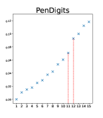
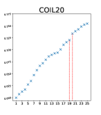
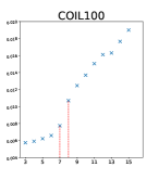
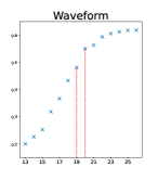
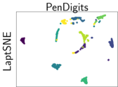
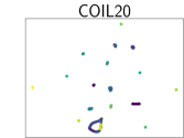
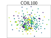
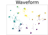
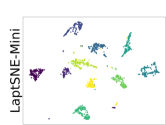
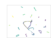
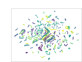
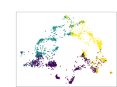
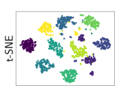
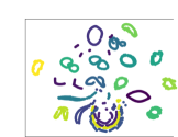
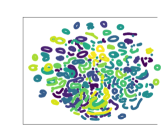
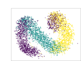
Figure 1. Row 1: First smallest eigenvalues of graph Laplacian for data $\mathbf{X}$ (From left to right: PenDigits, 11-th gap is large; COIL20, 19-th gap is large; COIL100, 7-th gap is large; Waveform, 19-th gap is large). Row 2-4: A qualitative comparison of LaptSNE, LaptSNE-Mini and t-SNE in visualizing the PenDigits, COIL20, COIL100 and Waveform datasets

We see that Waveform, COIL20, COIL100 and PenDigits are small datasets with no more than 10,000 samples while HAR, MNIST and Fashion-MNIST are large datasets with more than ten thousand samples. We will show the results on the small datasets and large datasets separately. The proposed LaptSNE and LaptSNE-Mini are compared with the following baselines.

• Vanilla t-SNE (Van der Maaten and Hinton, 2008): We implement t-SNE using the TSNE module in scikit-learn package (Pedregosa et al., 2011). To ensure a fair comparison, we remove the trick of exaggeration stage and set desired perplexity and number of iterations the same as LaptSNE.

• UMAP (McInnes et al., 2018a): We perform UMAP visualization using the latest umap-learn package (McInnes et al., 2018b). Specifically, we remain the parameters as default and set number of iterations the same as LaptSNE.

• Laplacian Eigenmaps (Belkin and Niyogi, 2003): We implement it as SpectralEmbedding module in the scikit-learn package (Pedregosa et al., 2011), where parameters are set as default.

• PCA (Jolliffe and Cadima, 2016): We use the LAPACK implementation of full SVD in the scikit-learn package (Pedregosa et al., 2011).

The implementation of our LaptSNE and LaptSNE-Mini are based on the scikit-learn package and gradient descent optimization.

Table 2. Comparison between LaptSNE, LaptSNE-Mini, t-SNE, UMAP, Eigenmaps and PCA on PenDigits, COIL20, COIL100 and Waveform: 1) $k$-NN classifier accuracy for different values of $k$ (McInnes et al., 2018a); 2) clustering performances in terms of NMI, SC and DBI based on the hyperparameter $\hat{k}$. Note: $\uparrow$ means the higher is better, whereas $\downarrow$ indicates the lower is better. The best value in each case is highlighted in bold.

	score	LaptSNE	LaptSNE-Mini	t-SNE	UMAP	Eigenmaps	PCA
PenDigits	10-nn $\uparrow$ 20-nn $\uparrow$ 40-nn $\uparrow$ 80-nn $\uparrow$ NMI $\uparrow$ SC $\uparrow$ DBI $\downarrow$	0.990 0.987 0.975 0.970 0.9084 0.7535 0.4064	0.989 0.989 0.966 0.952 0.8793 0.6742 0.4531	0.977 0.973 0.956 0.948 0.7148 0.4754 0.7121	0.988 0.983 0.972 0.956 0.8981 0.6010 0.5688	0.828 0.816 0.805 0.785 0.7869 0.6976 0.4532	0.710 0.682 0.671 0.660 0.5267 0.3936 0.7992
COIL20	10-nn $\uparrow$ 20-nn $\uparrow$ 40-nn $\uparrow$ 80-nn $\uparrow$ NMI $\uparrow$ SC $\uparrow$ DBI $\downarrow$	0.986 0.943 0.909 0.860  0.8723 0.7947 0.3251	0.897 0.895 0.874 0.844 0.8723 0.7947 0.3251	0.934 0.901 0.857 0.789 0.8286 0.5105 0.6866	0.901 0.885 0.877 0.822 0.8489 0.5689 0.5997	0.773 0.744 0.694 0.638 0.5527 0.5760 0.6394	0.754 0.732 0.677 0.578 0.6391 0.4750 0.7287
COIL100	10-nn $\uparrow$ 20-nn $\uparrow$ 40-nn $\uparrow$ 80-nn $\uparrow$ NMI $\uparrow$ SC $\uparrow$ DBI $\downarrow$	0.937 0.900 0.860 0.798 0.8601 0.6026 0.5497	0.936 0.907 0.861 0.792 0.8778 0.6001 0.5827	0.894 0.856 0.808 0.718 0.8694 0.5682 0.5841	0.832 0.810 0.779 0.735 0.8785 0.5126 0.6507	0.633 0.582 0.524 0.468 0.6727 0.4280 0.7500	0.626 0.59 0.538 0.483 0.4440 0.4253 0.7473
Waveform	10-nn $\uparrow$ 20-nn $\uparrow$ 40-nn $\uparrow$ 80-nn $\uparrow$ NMI $\uparrow$ SC $\uparrow$ DBI $\downarrow$	0.859 0.850 0.845 0.838 0.3863 0.4658 0.7692	0.859 0.853 0.844 0.841 0.3686 0.4811 0.6980	0.849 0.842 0.836 0.838 0.3506 0.4624 0.7349	0.850 0.849 0.843 0.841 0.3709 0.5121 0.6549	0.822 0.834 0.820 0.812 0.3679 0.6821 0.4113	0.846 0.838 0.833 0.832 0.3605 0.4997 0.6755

We will present both qualitative results and quantitative results in the comparison studies. We consider the following evaluation metrics.

• $k$-nearest neighbor classifier accuracy It measures the quantitative performance of the preservation of cluster information in the original space. With the hyper-parameter $k$ varying, we can also consider how structure preservation changes from purely local to more global. When computing the errors, the labels collected beforehand are assumed to contain the inherent cluster information. The metric has been used in many previous works of dimensionality reduction such as (McInnes et al., 2018a).

• Normalized Mutual Information (NMI)(Estévez et al., 2009) NMI is a widely-used metric for evaluating the performance of clustering algorithm. It scales between 0 (no mutual information) and 1 (perfect correlation). In this study, we compute NMI based on the ground-truth label and the clustering result of k-means on the low-dimensional embedding $\mathbf{Y}$, where k is set as the number of actual classes.

• Silhouette Coefficient (SC) (Rousseeuw, 1987) SC ranges from -1 to 1, measuring how distinct or well-separated a cluster is from other clusters. The score of SC is higher when clusters are dense and well separated. Similar to NMI, we compute SC using the result of k-means on $\mathbf{Y}$.

• Davies-Bouldin Index (DBI) (Davies and Bouldin, 1979) DBI calculates the ratio of within-cluster and between-cluster distances, and therefore, lower the score the better separation there is between clusters. Similar to NMI, we compute DBI using the result of k-means on $\mathbf{Y}$.

4.2. Results on Small Datasets

The eigenvalues of graph Laplacian in the original space implies the potential number of clusters. Therefore, we first investigate into the eigenvalue sequence of the Laplacian matrix corresponding to $\mathbf{P_{X}}$ in the original data space. For Waveform, PenDigits, COIL20 and COIL100 datasets, the Gaussian kernel with perplexity of 25 was used to construct $\mathbf{P_{X}}$. As shown in the first row of Figure 1, for COIL20, the gap between eigenvalues 19 and 20 are more distinguishable than others, although the gaps between eigenvalues 6 and 7 and between eigenvalues 8 and 9 are also large. As analyzed in Section 3.7, we prefer an overestimated cluster number and hence we set $\hat{k}=19$ for COIL20, even though the true cluster number is 20. Similarly, the estimated number of potential clusters in Waveform, PenDigits and COIL100 datasets are 19, 11 and 7 respectively. We do not require $\hat{k}=k$ because it is unrealistic in practice and our LaptSNE is not sensitive to $\hat{k}$. We will illustrate this point via using a wide range of $\hat{k}$ later.

As for the results, we first plot the two dimensional embedding colored with ground-truth label in Figure 1. We claim that the quality of embedding produced by LaptSNE and LaptSNE-Mini are better than t-SNE for the four small datasets, although the three algorithms are all powerful in preserving the local and global structures from the original space. LaptSNE and LaptSNE-Mini can shrink the clusters into compact clusters in a powerful cluster-contractive manner.

In Table 2, we quantitatively compare LaptSNE, LaptSNE-Mini, t-SNE, UMAP, Eigenmaps and PCA embedding with respect to the four evaluation metrics. We see that LaptSNE performs remarkably better on PenDigits and COIL20 among all the dimensional reduction methods. It performs at least as well as t-SNE on COIL100. Note that on Waveform, in terms of the SC and DBI metrics, Eigenmaps outperforms other methods, but in terms of NMI, Eigenmaps is outperformed by our LaptSNE. One possible reason is that SC and DBI are not effective enough to quantify the with-class and between-class differences of this dataset. In addition, NMI is more reliable than SC and DBI because it utilizes the true labels.

Evidently, the embedding quality of LaptSNE is better compared with t-SNE and UMAP at both local and non-local scales in terms of PenDigits and COIL20. As for COIL100, it provides largely comparable performance in embedding at local scales, but performs superior at non-local scales. Besides, as shown in Table 1 and Table 2, the proposed mini-batch based LaptSNE could remarkably save the computational time while maintaining good performance. In this way, LaptSNE-Mini could be considered as an efficient alternative when dealing with large datasets.

4.3. Results on Large Datasets

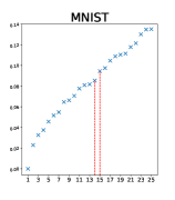
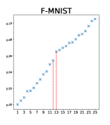
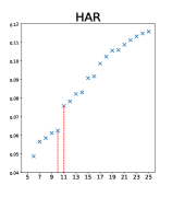
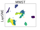
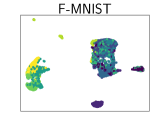
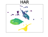
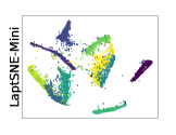
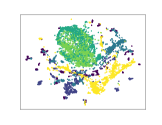
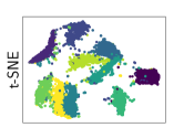
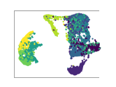
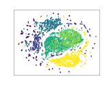
Figure 2. Row 1: Smallest few eigenvalues of graph Laplacian of each dataset (From left to right: MNIST, 14-th gap is large; Fashion-MNIST, 12-th gap is large; HAR, 10-th gap is large). Rows 2-4: Qualitative comparison of LaptSNE, LaptSNE-Mini and t-SNE in visualizing MNIST, Fashion-MNIST and HAR.

In the same way mentioned above, the largest eigengap of HAR, MNIST and FMNIST are estimated, which turns out to be 10, 14 and 12 respectively, shown by the first row of Figure 2. Since these are quite large datasets, we use the out-of-sample extension of LaptSNE proposed in Section 3.5. The neural network consists of 4 hidden layers of size $W=\left\{\left\lfloor\frac{2}{3}\right\rfloor D,\left\lfloor\frac{1}{2}\right\rfloor D,\left\lfloor\frac{1}{3}\right\rfloor D,\left\lfloor\frac{1}{5}\right\rfloor D\right\}$ where $D$ is the dimension of $\mathbf{X}$. The activation functions in the hidden layers are ReLU. The number of landmark points is 10000.

As shown in Figure 2, LaptSNE is more effective in capturing the latent cluster information than t-SNE. For instance, in the result of LaptSNE, the global relationships among different clusters of the digits in MNIST are more clearly identified and the clusters themselves are more compact.

Table 3. Comparison between LaptSNE, LaptSNE-Mini, t-SNE, UMAP, Eigenmaps and PCA on PenDigits, MNIST, Fashion-MNIST and HAR dataset: 1) $k$-NN classifier accuracy for different values of $k$ (McInnes et al., 2018a); 2) clustering performances in terms of NMI, SC and DBI based on the hyperparameter $\hat{k}$. Note: $\uparrow$ means the higher is better, whereas $\downarrow$ indicates the lower is better. The best value in each case is highlighted in bold.

	score	LaptSNE	LaptSNE-Mini	t-SNE	UMAP	Eigenmaps	PCA
MNIST	100-nn $\uparrow$ 200-nn $\uparrow$ 400-nn $\uparrow$ 800-nn $\uparrow$ NMI $\uparrow$ SC $\uparrow$ DBI $\downarrow$	0.943 0.940 0.937 0.935 0.7498 0.5886 0.5592	0.940 0.939 0.934 0.933 0.7340 0.5809 0.6038	0.941 0.937 0.933 0.932 0.6221 0.4178 0.7268	0.943 0.941 0.935 0.930 0.6892 0.4949 0.7476	0.695 0.680 0.659 0.635 0.3101 0.3464 0.8447	0.548 0.524 0.503 0.497 0.3595 0.3519 0.8487
F-MNIST	100-nn $\uparrow$ 200-nn $\uparrow$ 400-nn $\uparrow$ 800-nn $\uparrow$ NMI $\uparrow$ SC $\uparrow$ DBI $\downarrow$	0.787 0.768 0.762 0.753 0.6009 0.6299 0.4679	0.783 0.760 0.758 0.753 0.6004 0.6298 0.4680	0.782 0.771 0.762 0.754 0.5905 0.6113 0.5035	0.754 0.738 0.718 0.697 0.6051 0.5325 0.6557	0.695 0.675 0.652 0.636 0.4595 0.4789 0.7410	0.606 0.583 0.574 0.563 0.4311 0.4100 0.7709
HAR	100-nn $\uparrow$ 200-nn $\uparrow$ 400-nn $\uparrow$ 800-nn $\uparrow$ NMI $\uparrow$ SC $\uparrow$ DBI $\downarrow$	0.931 0.924 0.910 0.884 0.734 0.4667 0.7973	0.918 0.906 0.893 0.870 0.6015 0.4059 0.8046	0.915 0.909 0.897 0.840 0.4601 0.3893 0.8446	0.893 0.881 0.860 0.852 0.6878 0.5275 0.7376	0.769 0.746 0.739 0.722 0.6289 0.7657 0.4756	0.650 0.639 0.632 0.619 0.4590 0.4455 0.7371

In Table 3 we present the NMI, DC, DBI and k-NN scores on MNIST, Fashion-MNIST and HAR. LaptSNE established comparable performance with t-SNE on Fashion-MNIST at both local and non-local scales, but notably better than UMAP. For MNIST, LaptSNE is slightly better than other algorithms when k varies from 100 to 400, but has significantly higher accuracy for k values of 800.

As evidenced by this comparison, LaptSNE provides largely comparabe performance across large datasets both qualitatively and quantitatively. The success of LaptSNE may be owing to the theory proved in (Cai and Ma, 2021) that the low-dimensional map in t-SNE algorithm converges cluster-wise towards some limit points in $\mathbb{R}^{2}$, only depending on the initialization, and each associated with a connected component of the underlying graph. According to our experiments, the Laplacian regularization term helps strengthen this process without undermining the fine properties of t-SNE.

4.4. Sensitivity Analysis

We analyze the sensitivity of LaptSNE to the hyperparameters $\lambda$ and $\hat{k}$ qualitatively and quantitatively. For example, Figure 3 presents the k-NN score (k=20) of LaptSNE with different $\hat{k}$ and $\lambda$ on COIL20. We notice that large scale of $\lambda$ (e.g. 1e-1) would crush the performance but smaller ones from 1e-2 to 1e-6 could yield results even better than that of the vanilla t-SNE ($\lambda=0$). The hyperparameter $\hat{k}$ may fluctuate the performance in a non-monotonic manner. For the order of $\hat{k}$ where a large eigengap exists, the k-NN scores are the best. This indicates the importance of tuning the estimated number of potential cluster $\hat{k}$ according to the eigenvalues of graph Laplacian in the original space. When tuning $\hat{k}=19$ and $\lambda=$1e-4, LaptSNE has the highest k-NN score (k=20) as Table 2 shows, and the embedding layout is cluster-contractive, which consists of many circles and lines in Figure 1.

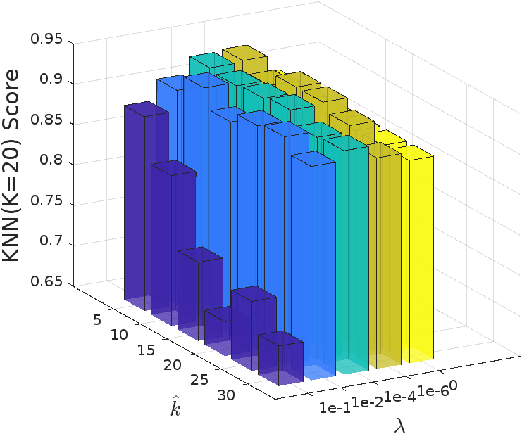
Figure 3. K-NN scores (k=20) on the COIL20 dataset: LaptSNE result with different $\lambda$ (ranging from 0 to 1e-1) and estimated number of potential cluster $\hat{k}$ (ranging from 5 to 30).

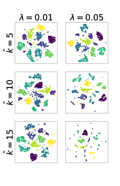
Figure 4. Variation of LaptSNE embedding with different hyperparameters $\hat{k}$ and $\lambda$ on the PenDigits dataset.

In Figure 4, it is shown obviously that the clusters shrink with the increase of $\hat{k}$. Besides, the experiment further supports the interaction effect between the estimated number of potential clusters $\hat{k}$ and the tuning parameter $\lambda$: relatively larger $\lambda$ and $\hat{k}$ can produce more compact clusters.

4.5. Trajectory of LaptSNE

We discover that LaptSNE outperforms t-SNE in the early stage of iterations. As Figure 6 illustrates, the lower-dimensional embeddings of LaptSNE start from the same intialization as t-SNE but expand in a cluster-contractive manner, which leads to a well-clustered layout in the end.

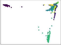
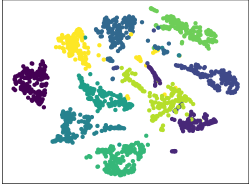
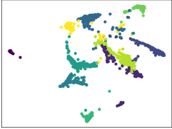
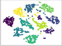
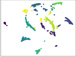
Figure 5. A comparison of t-SNE and LaptSNE in the first 50 iterations on PenDigits. (Left: t-SNE, Right: LaptSNE; Row 1 is the initial stage, Row 2 to Row 4 are iteration 10, 30, 50)

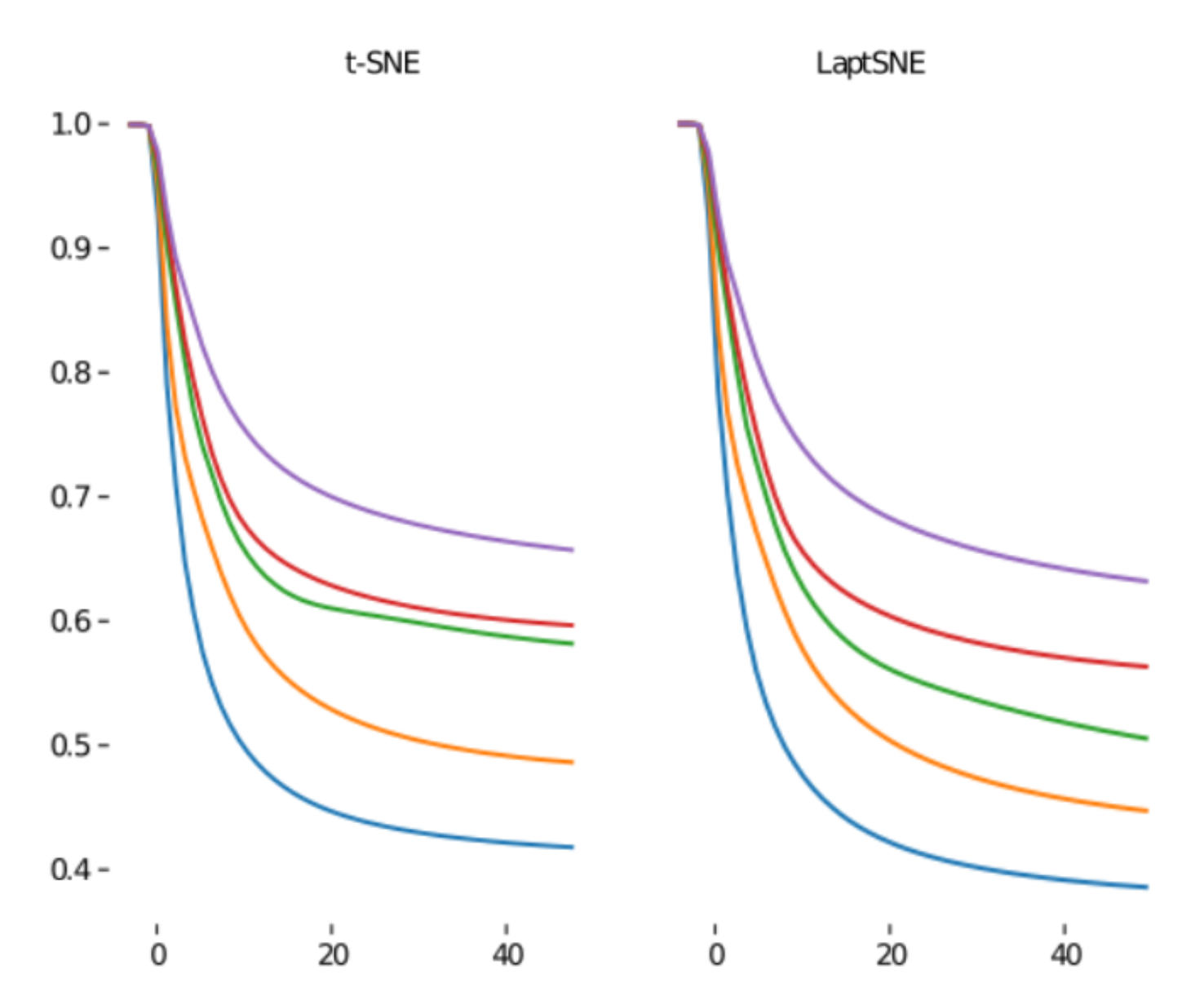
Figure 6. Part of the eigenvalues of T-Student kernel graph in the 2-dimensional embeddings of LaptSNE and t-SNE (in different iterations) on PenDigits. The green curve stands for the 11-th eigenvalue.

Note that, shown in Figure 6, the clusters in the embeddings of LaptSNE are more distinguishable than those in the embeddings of t-SNE. This is consistent with the fact that, shown in Figure 6, the gap between the 11-th and 12-th eigenvalues of the lower-dimensional representation’s graph Laplacian is increasingly large during the iteration of LaptSNE, compared with vanilla t-SNE.

5. Conclusions

This work provided a new NLDR method called LaptSNE and its several extensions for high-dimensional data visualization. The proposed methods generate cluster-informative low-dimensional embedding and outperform t-SNE and UMAP visually and quantitatively on seven benchmark datasets. It should be pointed out that the proposed method can be adapted to other NLDR methods such as UMAP to boost the visualization performance.

Appendix A Appendices

A.1. Proof for Proposition 1

Denote $\hat{\mathcal{L}}_{2}(\mathbf{Y}|\mathbf{Y}_{t-1})=\hat{\mathcal{L}}_{2}(\mathbf{Y})$. Using the definitions of ${\mathcal{L}}_{2}(\mathbf{Y})$ and $\hat{\mathcal{L}}_{2}(\mathbf{Y})$, we have

(28) $${\mathcal{L}}_{2}(\mathbf{Y})\leq\hat{\mathcal{L}}_{2}(\mathbf{Y}|\mathbf{Y}_{t-1})$$

and

(29) $$\mathcal{L}_{1}(\mathbf{Y})+{\mathcal{L}}_{2}(\mathbf{Y})\leq\mathcal{L}_{1}(\mathbf{Y})+\hat{\mathcal{L}}_{2}(\mathbf{Y}|\mathbf{Y}_{t-1}).$$

It follows that

(30) $$\mathcal{L}_{1}(\mathbf{Y}_{t})+{\mathcal{L}}_{2}(\mathbf{Y}_{t})\leq\mathcal{L}_{1}(\mathbf{Y}_{t})+\hat{\mathcal{L}}_{2}(\mathbf{Y}_{t}|\mathbf{Y}_{t-1})$$

Supposing $\mathcal{L}_{1}(\mathbf{Y}_{t})+\hat{\mathcal{L}}_{2}(\mathbf{Y}_{t})\leq\mathcal{L}_{1}(\mathbf{Y}_{t-1})+\hat{\mathcal{L}}_{2}(\mathbf{Y}_{t-1})-\Delta_{t}$ and combining (30), we arrive at

(31) $$\mathcal{L}_{1}(\mathbf{Y}_{t})+{\mathcal{L}}_{2}(\mathbf{Y}_{t})\leq\mathcal{L}_{1}(\mathbf{Y}_{t-1})+\hat{\mathcal{L}}_{2}(\mathbf{Y}_{t-1})-\Delta_{t}.$$

Invoking the fact ${\mathcal{L}}_{2}(\mathbf{Y}_{t-1})=\hat{\mathcal{L}}_{2}(\mathbf{Y}_{t-1}|\mathbf{Y}_{t-1})=\bar{\mathcal{L}}_{2}(\mathbf{Y}_{t-1})$ into (31), we obtain

(32) $$\mathcal{L}_{1}(\mathbf{Y}_{t})+{\mathcal{L}}_{2}(\mathbf{Y}_{t})\leq\mathcal{L}_{1}(\mathbf{Y}_{t-1})+{\mathcal{L}}_{2}(\mathbf{Y}_{t-1})-\Delta_{t}.$$

Because $\nabla\hat{\mathcal{L}}(\mathbf{Y})$ is $L$-Lipschitz continuous, we have

(33) $$\hat{\mathcal{L}}(\mathbf{Y})\leq \hat{\mathcal{L}}(\mathbf{Y}_{t-1})+\left\langle\nabla\hat{\mathcal{L}}(\mathbf{Y}_{t-1}),\mathbf{Y}-\mathbf{Y}_{t-1}\right\rangle$$

$$+\frac{L}{2}\|\mathbf{Y}-\mathbf{Y}_{t-1}\|_{F}^{2}.$$

Invoking the update of $\mathbf{Y}$, i.e., $\mathbf{Y}_{t}=\mathbf{Y}_{t-1}-\alpha\nabla\hat{\mathcal{L}}(\mathbf{Y}_{t-1})$, into (33), we get

(34) $$\hat{\mathcal{L}}(\mathbf{Y}_{t})\leq\hat{\mathcal{L}}(\mathbf{Y}_{t-1})-\left(\frac{1}{\alpha}-\frac{L}{2}\right)\left\|\mathbf{Y}_{t}-\mathbf{Y}_{t-1}\right\|_{F}^{2}$$

It means

(35) $$\begin{aligned} \Delta_{t}=\left(\frac{1}{\alpha}-\frac{L}{2}\right)\left\|\mathbf{Y}_{t}-\mathbf{Y}_{t-1}\right\|_{F}^{2}\end{aligned}.$$

Now combining (32) and (35), we arrive at

(36) $$\mathcal{L}(\mathbf{Y}_{t})\leq\mathcal{L}(\mathbf{Y}_{t-1})-\left(\frac{1}{\alpha}-\frac{L}{2}\right)\left\|\mathbf{Y}_{t}-\mathbf{Y}_{t-1}\right\|_{F}^{2}.$$

Sum up (37) from $t=1$ to $t=T$, we have

(37) $$\mathcal{L}(\mathbf{Y}_{T})\leq\mathcal{L}(\mathbf{Y}_{0})-\left(\frac{1}{\alpha}-\frac{L}{2}\right)\sum_{t=1}^{T}\left\|\mathbf{Y}_{t}-\mathbf{Y}_{t-1}\right\|_{F}^{2}.$$

This finished the proof.

A.2. Gradient Computation for Gaussian Kernel

For Gaussian kernel with $\sigma_{i}$ for $\mathbf{x}_{i}$,

(38) $$K_{ij}=\exp\left(-\frac{\|\mathbf{y_{i}}-\mathbf{y_{j}}\|^{2}}{2\sigma_{i}^{2}}\right).$$

As the adjacent matrix $\mathbf{Q}$ is symmetric,

(39) $$q_{ji}=q_{ij}=\frac{K_{ij}+K_{ji}}{2}$$

(40) $$\frac{\partial\mathrm{Tr}(\mathbf{V^{\top}LV})}{\partial\mathbf{Y}}$$

$$=\sum_{m}\sum_{n}(U^{0}_{mn}+U^{1}_{mn}+U^{2}_{mn})\odot\frac{\partial q_{mn}}{\partial\mathbf{Y}}$$

$$=\sum_{m}\sum_{n}(U^{0}_{mn}+U^{1}_{mn}+U^{2}_{mn})\sum_{i}\sum_{j}\frac{\partial q_{mn}}{\partial K_{ij}}\frac{\partial K_{ij}}{\partial\mathbf{Y}}$$

$$=\sum_{i}\sum_{j}(\sum_{m}\sum_{n}(U^{0}_{mn}+U^{1}_{mn}+U^{2}_{mn})\frac{\partial q_{mn}}{\partial K_{ij}})\odot\frac{\partial K_{ij}}{\partial\mathbf{Y}}$$

$$=\sum_{i}\sum_{j}[\frac{1}{2}(U^{0}_{ij}+U^{1}_{ij}+U^{2}_{ij})+\frac{1}{2}(U^{0}_{ji}+U^{1}_{ji}+U^{2}_{ji})]\odot\frac{\partial K_{ij}}{\partial\mathbf{Y}}$$

$$=\sum_{i}\sum_{j}(U^{0}_{ij}+U^{1}_{ij}+U^{2}_{ij})\odot\frac{\partial K_{ij}}{\partial\mathbf{Y}}$$

In case of Gaussian kernel matrix, we can calculate the gradient on element $\mathbf{y_{a}}$ of $\mathbf{Y}$ as below.

(41) $$\frac{\partial\mathrm{Tr}(\mathbf{V^{\top}LV})}{\partial\mathbf{y_{a}}}$$

$$=\sum_{i}\sum_{j}\frac{\partial\mathrm{Tr}(\mathbf{V^{\top}LV})}{\partial K_{ij}}\frac{\partial K_{ij}}{\partial\mathbf{y_{a}}}$$

$$=\begin{cases}\frac{1}{-\sigma_{a}^{2}}\sum_{j}\frac{\partial\mathrm{Tr}(\mathbf{V^{\top}LV})}{\partial K_{aj}}K_{aj})(\mathbf{y_{a}}-\mathbf{y_{j}})&i=a\\ \sum_{i}\frac{1}{-\sigma_{i}^{2}}\frac{\partial\mathrm{Tr}(\mathbf{V^{\top}LV})}{\partial K_{ia}}K_{ia})(\mathbf{y_{a}}-\mathbf{y_{i}})&j=a\end{cases}$$

$$\left(\text{let}\quad U_{ij}=\frac{U^{0}_{ij}+U^{1}_{ij}+U^{2}_{ij}}{\sigma_{i}^{2}}\odot K_{ij}\right)$$

$$=\begin{cases}\sum_{j}U_{aj}\mathbf{y_{j}}-\mathbf{y_{a}}\sum_{j}U_{aj}&i=a\\ \sum_{i}U_{ia}\mathbf{y_{i}}-\mathbf{y_{a}}\sum_{i}U_{ia}&j=a\\ \end{cases}$$

$$\text{so,}\quad\frac{\partial\mathrm{Tr}(\mathbf{V^{\top}LV})}{\partial\mathbf{Y}}$$

$$=\begin{cases}\mathbf{UY}-\mathbf{Y}\odot\mathbf{C}\\ \mathbf{U}^{\top}\mathbf{Y}-\mathbf{Y}\odot\mathbf{C}^{\prime}\end{cases}$$

$$\text{where,}\quad\mathbf{C}=\mathbf{U}\mathbf{1}_{N}\mathbf{1}_{d}^{\top}\quad\mathbf{C}^{\prime}=\mathbf{1}_{d}\mathbf{1}_{N}^{\top}\mathbf{U}$$

To sum up, the calculation of gradient $\frac{\partial\mathrm{Tr}(\mathbf{V^{\top}LV})}{\partial\mathbf{Y}}$ is

(42) $$\frac{\partial\mathrm{Tr}(\mathbf{V^{\top}LV})}{\partial\mathbf{Y}}=(\mathbf{U}+\mathbf{U}^{\top})\mathbf{Y}-\mathbf{Y}\odot(\mathbf{C}+\mathbf{C}^{\prime}).$$

A.3. More Numerical Results

In section 4, NMI, SC, DBI scores of LaptSNE outperform others in most cases. As for $k$-means on low-dimensional embedding, we can choose $k$ as the estimated number of potential cluster $\hat{k}$ to examine LaptSNE, rather than the exact number of the ground-truth labels. The results in terms of NMI, SC, and DBI on the seven datasets are reported in Table 4. Our LaptSNE and LaptSNE-Mini still outperform the baselines in most cases.

Table 4. Comparison of clustering performances (NMI, SC and DBI) between LaptSNE, LaptSNE-Mini, t-SNE, UMAP, Eigenmaps and PCA on all datasets. Note: $\uparrow$ means the higher is better, whereas $\downarrow$ indicates the lower is better. The best value in each case is highlighted in bold.

	score	LaptSNE	LaptSNE-Mini	t-SNE	UMAP	Eigenmaps	PCA
PenDigits	NMI $\uparrow$ SC $\uparrow$ DBI $\downarrow$	0.9284 0.7605 0.3806	0.8901 0.6920 0.4175	0.7679 0.4887 0.7228	0.9083 0.6115 0.5407	0.7804 0.6832 0.4784	0.5164 0.3918 0.7933
COIL20	NMI $\uparrow$ SC $\uparrow$ DBI $\downarrow$	0.8787 0.8023 0.2863	0.8785 0.8021 0.2866	0.8218 0.5024 0.6741	0.8458 0.5700 0.5935	0.5477 0.5720 0.6499	0.5527 0.5760 0.6394
COIL100	NMI $\uparrow$ SC $\uparrow$ DBI $\downarrow$	0.5119 0.3762 0.7909	0.5035 0.3721 0.7923	0.4741 0.3572 0.7846	0.5362 0.3659 0.8021	0.4532 0.4384 0.7899	0.4440 0.4095 0.7371
Wavform	NMI $\uparrow$ SC $\uparrow$ DBI $\downarrow$	0.3555 0.9185 0.1100	0.3529 0.7367 0.3634	0.3592 0.3535 0.8586	0.3633 0.3480 0.8483	0.3101 0.3464 0.8447	0.3589 0.4633 0.6763
MNIST	NMI $\uparrow$ SC $\uparrow$ DBI $\downarrow$	0.7278 0.6147 0.4885	0.7017 0.6111 0.5264	0.6129 0.3908 0.8074	0.7004 0.4882 0.7182	0.3137 0.3435 0.8247	0.3492 0.3435 0.8247
F-MNIST	NMI $\uparrow$ SC $\uparrow$ DBI $\downarrow$	0.5910 0.6114 0.5043	0.5818 0.5125 0.6680	0.5221 0.4178 0.7068	0.5881 0.5093 0.7055	0.4565 0.4734 0.7244	0.4261 0.3815 0.8280
HAR	NMI $\uparrow$ SC $\uparrow$ DBI $\downarrow$	0.6296 0.4586 0.7764	0.5689 0.3797 0.8363	0.4602 0.3623 0.8446	0.6179 0.4151 0.8311	0.5835 0.7413 0.5168	0.4245 0.3906 0.8153

A.4. More Qualitative Comparison

Figure 7 shows the qualitative comparison of LaptSNE with other methods. LaptSNE has comparable performance with UMAP on visual results, and it is significantly better than other methods.

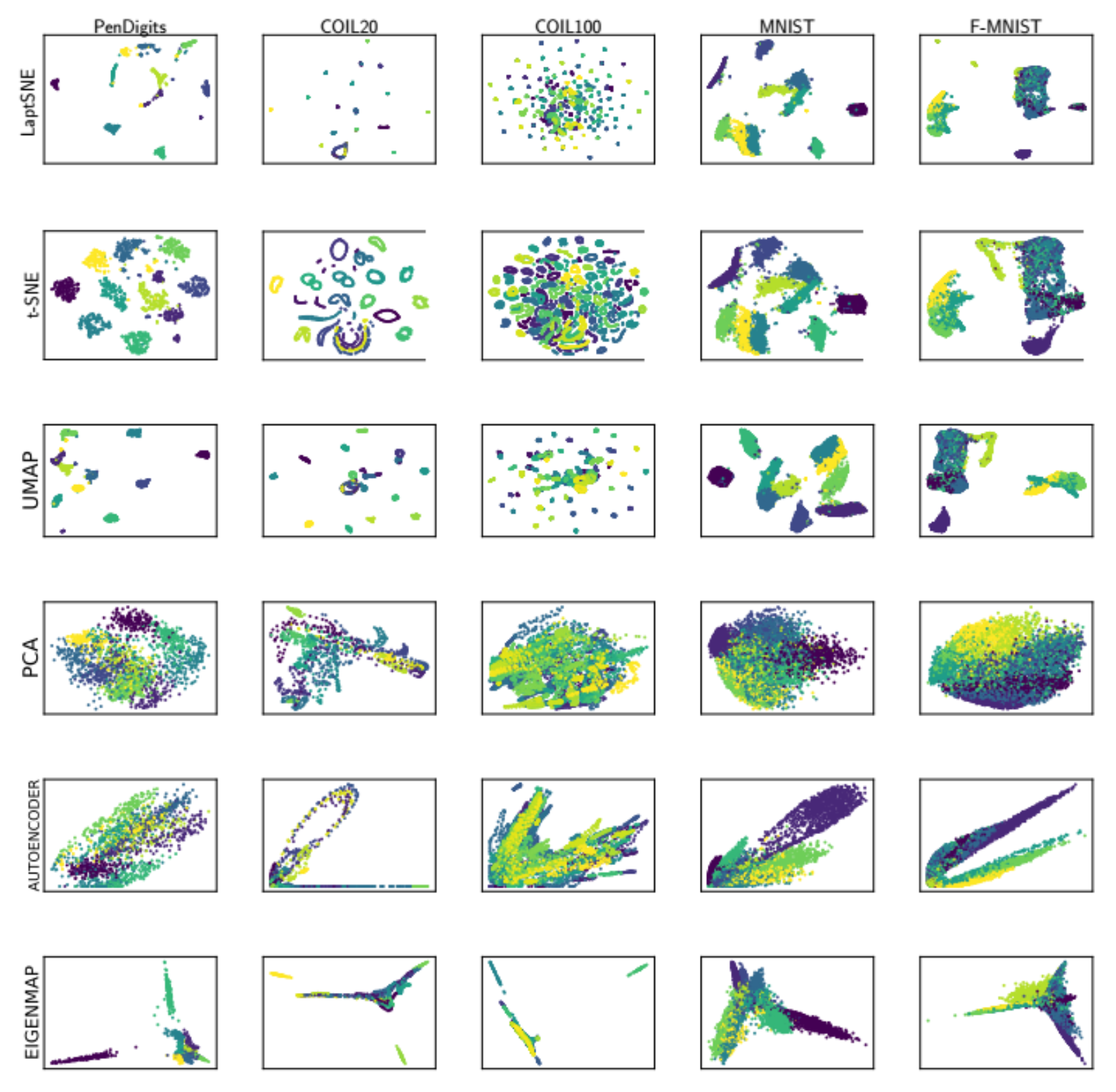
Figure 7. A comparison of LaptSNE and other dimensionality reduction methods for all datasets.

References

- (1)
- Arora et al. (2018) Sanjeev Arora, Wei Hu, and Pravesh K. Kothari. 2018. An Analysis of the t-SNE Algorithm for Data Visualization. In Proceedings of the 31st Conference On Learning Theory (Proceedings of Machine Learning Research, Vol. 75), Sébastien Bubeck, Vianney Perchet, and Philippe Rigollet (Eds.). PMLR, 1455–1462. https://proceedings.mlr.press/v75/arora18a.html
- Baker (1977) Christopher TH Baker. 1977. The numerical treatment of integral equations. Oxford University Press.
- Belkin and Niyogi (2003) Mikhail Belkin and Partha Niyogi. 2003. Laplacian eigenmaps for dimensionality reduction and data representation. Neural computation 15, 6 (2003), 1373–1396.
- Breiman et al. (2017) Leo Breiman, Jerome H Friedman, Richard A Olshen, and Charles J Stone. 2017. Classification and regression trees. Routledge.
- Buitinck et al. (2013) Lars Buitinck, Gilles Louppe, Mathieu Blondel, Fabian Pedregosa, Andreas Mueller, Olivier Grisel, Vlad Niculae, Peter Prettenhofer, Alexandre Gramfort, Jaques Grobler, et al. 2013. API design for machine learning software: experiences from the scikit-learn project. arXiv preprint arXiv:1309.0238 (2013).
- Cai and Ma (2021) T Tony Cai and Rong Ma. 2021. Theoretical Foundations of t-SNE for Visualizing High-Dimensional Clustered Data. arXiv preprint arXiv:2105.07536 (2021).
- Carreira-Perpinán (2010) Miguel A Carreira-Perpinán. 2010. The Elastic Embedding Algorithm for Dimensionality Reduction.. In ICML, Vol. 10. Citeseer, 167–174.
- Chatzimparmpas et al. (2020) Angelos Chatzimparmpas, Rafael M Martins, and Andreas Kerren. 2020. t-viSNE: Interactive Assessment and Interpretation of t-SNE Projections. IEEE transactions on visualization and computer graphics 26, 8 (2020), 2696–2714.
- Chung and Graham (1997) Fan RK Chung and Fan Chung Graham. 1997. Spectral graph theory. Number 92. American Mathematical Soc.
- Davies and Bouldin (1979) David L Davies and Donald W Bouldin. 1979. A cluster separation measure. IEEE transactions on pattern analysis and machine intelligence 2 (1979), 224–227.
- DeMers and Cottrell (1992) David DeMers and Garrison Cottrell. 1992. Non-linear dimensionality reduction. Advances in neural information processing systems 5 (1992).
- Deng (2012) Li Deng. 2012. The mnist database of handwritten digit images for machine learning research [best of the web]. IEEE Signal Processing Magazine 29, 6 (2012), 141–142.
- Donoho (2017) David Donoho. 2017. 50 years of data science. Journal of Computational and Graphical Statistics 26, 4 (2017), 745–766.
- Estévez et al. (2009) Pablo A Estévez, Michel Tesmer, Claudio A Perez, and Jacek M Zurada. 2009. Normalized mutual information feature selection. IEEE Transactions on neural networks 20, 2 (2009), 189–201.
- Fisher (1936) Ronald A Fisher. 1936. The use of multiple measurements in taxonomic problems. Annals of eugenics 7, 2 (1936), 179–188.
- Gisbrecht et al. (2015) Andrej Gisbrecht, Alexander Schulz, and Barbara Hammer. 2015. Parametric nonlinear dimensionality reduction using kernel t-SNE. Neurocomputing 147 (2015), 71–82.
- Hastie and Stuetzle (1989) Trevor Hastie and Werner Stuetzle. 1989. Principal curves. J. Amer. Statist. Assoc. 84, 406 (1989), 502–516.
- Hinton and Roweis (2002) Geoffrey Hinton and Sam T Roweis. 2002. Stochastic neighbor embedding. In NIPS, Vol. 15. Citeseer, 833–840.
- Hinton and Salakhutdinov (2006) Geoffrey E Hinton and Ruslan R Salakhutdinov. 2006. Reducing the dimensionality of data with neural networks. science 313, 5786 (2006), 504–507.
- Jolliffe and Cadima (2016) Ian T Jolliffe and Jorge Cadima. 2016. Principal component analysis: a review and recent developments. Philosophical Transactions of the Royal Society A: Mathematical, Physical and Engineering Sciences 374, 2065 (2016), 20150202.
- Kobak and Berens (2019) Dmitry Kobak and Philipp Berens. 2019. The art of using t-SNE for single-cell transcriptomics. Nature communications 10, 1 (2019), 1–14.
- Kohonen (1982) Teuvo Kohonen. 1982. Self-organized formation of topologically correct feature maps. Biological cybernetics 43, 1 (1982), 59–69.
- Li et al. (2017) Wentian Li, Jane E Cerise, Yaning Yang, and Henry Han. 2017. Application of t-SNE to human genetic data. Journal of bioinformatics and computational biology 15, 04 (2017), 1750017.
- Linderman et al. (2019) George C Linderman, Manas Rachh, Jeremy G Hoskins, Stefan Steinerberger, and Yuval Kluger. 2019. Fast interpolation-based t-SNE for improved visualization of single-cell RNA-seq data. Nature methods 16, 3 (2019), 243–245.
- McInnes et al. (2018a) Leland McInnes, John Healy, and James Melville. 2018a. Umap: Uniform manifold approximation and projection for dimension reduction. arXiv preprint arXiv:1802.03426 (2018).
- McInnes et al. (2018b) Leland McInnes, John Healy, Nathaniel Saul, and Lukas Grossberger. 2018b. UMAP: Uniform Manifold Approximation and Projection. The Journal of Open Source Software 3, 29 (2018), 861.
- Nene et al. (1996a) SA Nene, SK Nayar, and H Murase. 1996a. Columbia university image library (coil-20). Technical Report CUCS-005-96 (1996).
- Nene et al. (1996b) Sameer A Nene, Shree K Nayar, Hiroshi Murase, et al. 1996b. Columbia object image library (coil-100). (1996).
- Pearson (1901) Karl Pearson. 1901. LIII. On lines and planes of closest fit to systems of points in space. The London, Edinburgh, and Dublin philosophical magazine and journal of science 2, 11 (1901), 559–572.
- Pedregosa et al. (2011) F. Pedregosa, G. Varoquaux, A. Gramfort, V. Michel, B. Thirion, O. Grisel, M. Blondel, P. Prettenhofer, R. Weiss, V. Dubourg, J. Vanderplas, A. Passos, D. Cournapeau, M. Brucher, M. Perrot, and E. Duchesnay. 2011. Scikit-learn: Machine Learning in Python. Journal of Machine Learning Research 12 (2011), 2825–2830.
- Pezzotti et al. (2016) Nicola Pezzotti, Boudewijn PF Lelieveldt, Laurens Van Der Maaten, Thomas Höllt, Elmar Eisemann, and Anna Vilanova. 2016. Approximated and user steerable tSNE for progressive visual analytics. IEEE transactions on visualization and computer graphics 23, 7 (2016), 1739–1752.
- Reyes-Ortiz et al. (2013) Jorge Luis Reyes-Ortiz, Alessandro Ghio, Xavier Parra, Davide Anguita, Joan Cabestany, and Andreu Catala. 2013. Human Activity and Motion Disorder Recognition: towards smarter Interactive Cognitive Environments.. In ESANN. Citeseer.
- Rousseeuw (1987) Peter J Rousseeuw. 1987. Silhouettes: a graphical aid to the interpretation and validation of cluster analysis. Journal of computational and applied mathematics 20 (1987), 53–65.
- Roweis and Saul (2000) Sam T Roweis and Lawrence K Saul. 2000. Nonlinear dimensionality reduction by locally linear embedding. science 290, 5500 (2000), 2323–2326.
- Sammon (1969) John W Sammon. 1969. A nonlinear mapping for data structure analysis. IEEE Transactions on computers 100, 5 (1969), 401–409.
- Schölkopf et al. (1998) Bernhard Schölkopf, Alexander Smola, and Klaus-Robert Müller. 1998. Nonlinear component analysis as a kernel eigenvalue problem. Neural computation 10, 5 (1998), 1299–1319.
- Souza (2010) César R Souza. 2010. Kernel functions for machine learning applications. Creative Commons Attribution-Noncommercial-Share Alike 3 (2010), 29.
- Tenenbaum et al. (2000) Joshua B Tenenbaum, Vin De Silva, and John C Langford. 2000. A global geometric framework for nonlinear dimensionality reduction. science 290, 5500 (2000), 2319–2323.
- Vaida (2005) Florin Vaida. 2005. Parameter convergence for EM and MM algorithms. Statistica Sinica (2005), 831–840.
- Van Der Maaten (2014) Laurens Van Der Maaten. 2014. Accelerating t-SNE using tree-based algorithms. The Journal of Machine Learning Research 15, 1 (2014), 3221–3245.
- Van der Maaten and Hinton (2008) Laurens Van der Maaten and Geoffrey Hinton. 2008. Visualizing data using t-SNE. Journal of machine learning research 9, 11 (2008).
- Xiao et al. (2017) Han Xiao, Kashif Rasul, and Roland Vollgraf. 2017. Fashion-mnist: a novel image dataset for benchmarking machine learning algorithms. arXiv preprint arXiv:1708.07747 (2017).
- Xie et al. (2011) Bo Xie, Yang Mu, Dacheng Tao, and Kaiqi Huang. 2011. m-SNE: Multiview stochastic neighbor embedding. IEEE Transactions on Systems, Man, and Cybernetics, Part B (Cybernetics) 41, 4 (2011), 1088–1096.
- Yang et al. (2009) Zhirong Yang, Irwin King, Zenglin Xu, and Erkki Oja. 2009. Heavy-tailed symmetric stochastic neighbor embedding. Advances in neural information processing systems 22 (2009), 2169–2177.