On Computing Probabilistic Explanations
for Decision Trees

Abstract

Formal XAI (explainable AI) is a growing area that focuses on computing explanations with mathematical guarantees for the decisions made by ML models. Inside formal XAI, one of the most studied cases is that of explaining the choices taken by decision trees, as they are traditionally deemed as one of the most interpretable classes of models. Recent work has focused on studying the computation of sufficient reasons, a kind of explanation in which given a decision tree $T$ and an instance ${\bm{x}}$, one explains the decision $T({\bm{x}})$ by providing a subset ${\bm{y}}$ of the features of ${\bm{x}}$ such that for any other instance ${\bm{z}}$ compatible with ${\bm{y}}$, it holds that $T({\bm{z}})=T({\bm{x}})$, intuitively meaning that the features in ${\bm{y}}$ are already enough to fully justify the classification of ${\bm{x}}$ by $T$. It has been argued, however, that sufficient reasons constitute a restrictive notion of explanation. For such a reason, the community has started to study their probabilistic counterpart, in which one requires that the probability of $T({\bm{z}})=T({\bm{x}})$ must be at least some value $\delta\in(0,1]$, where ${\bm{z}}$ is a random instance that is compatible with ${\bm{y}}$. Our paper settles the computational complexity of $\delta$-sufficient-reasons over decision trees, showing that both (1) finding $\delta$-sufficient-reasons that are minimal in size, and (2) finding $\delta$-sufficient-reasons that are minimal inclusion-wise, do not admit polynomial-time algorithms (unless $\text{\rm PTIME}=\text{\rm NP}$). This is in stark contrast with the deterministic case ($\delta=1$) where inclusion-wise minimal sufficient-reasons are easy to compute. By doing this, we answer two open problems originally raised by Izza et al., and extend the hardness of explanations for Boolean circuits presented by Wäldchen et al. to the more restricted case of decision trees. On the positive side, we identify structural restrictions of decision trees that make the problem tractable, and show how SAT solvers might be able to tackle these problems in practical settings.

1 Introduction

Context.

The trust that AI models generate in people has been repetitively linked to our ability of explaining the decision of said models (Arrieta et al., 2020), thus suggesting the area of explainable AI (XAI) as fundamental for the deployment of trustworthy models. A sub-area of explainability that has received considerable attention over the last years, showing quick progress in theoretical and practical terms, is that of local explanations, i.e., explanations for the outcome of a particular input to an ML model after the model has been trained. Several queries and scores have been proposed to specify explanations of this kind. These include, e.g., queries based on prime implicants (Shih et al., 2018) or anchors (Ribeiro et al., 2018), which are parts of an instance that are sufficient to explain its classification, as well as scores that intend to quantify the impact of a single feature in the output of such a classification (Lundberg and Lee, 2017; Yan and Procaccia, 2021).

A remarkable achievement of this area of research has been the development of formal notions of explainability. The benefits brought about by this principled approach have been highlighted, in a very thorough and convincing way, in a recent survey by Marques-Silva and Ignatiev (2022). A prime example of this kind of approach is given by sufficient reasons, which are also known as prime implicant explanations (Shih et al., 2018) or abductive explanations (Ignatiev and Marques-Silva, 2021).

Given an ML model $\mathcal{M}$ of dimension $n$ and a Boolean input instance ${\bm{x}}\in\{0,1\}^{n}$, a sufficient reason for ${\bm{x}}$ under $\mathcal{M}$ is a subset ${\bm{y}}$ of the features of ${\bm{x}}$, such that any instance ${\bm{z}}$ compatible with ${\bm{y}}$ receives the same classification result as ${\bm{x}}$ on $\mathcal{M}$. In more intuitive words, ${\bm{y}}$ is a sufficient reason for ${\bm{x}}$ under $\mathcal{M}$ if the features in ${\bm{y}}$ suffices to explain the output of $\mathcal{M}$ on ${\bm{x}}$. In the formal explainability approach, one then aims to find sufficient reasons ${\bm{y}}$ that satisfy one of the following optimality criteria: (a) they are minimum, i.e., there are no sufficient reasons with fewer features than ${\bm{y}}$, or (b) they are minimal, i.e., there are no sufficient reasons that are strictly contained in ${\bm{y}}$.

Problem.

In the last few years, the XAI community has studied for which Boolean ML models the problem of computing (minimum or minimal) sufficient reasons is computationally tractable and for which it is computationally hard (see, e.g., (Marques-Silva et al., 2020; Barceló et al., 2020; Marques-Silva et al., 2021)). It has been argued, however, that for practical applications sufficient reasons might be too rigid, as they are specified under worst-case conditions. That is, ${\bm{y}}$ is a sufficient reason for ${\bm{x}}$ under $\mathcal{M}$ if every “completion” of ${\bm{y}}$ is classified by $\mathcal{M}$ in the same way as ${\bm{x}}$. As several authors have noted already, there is a natural way in which this notion can be relaxed in order to become more suitable for real-world explainability tasks: Instead of asking for each completion of ${\bm{y}}$ to yield the same result as ${\bm{x}}$ on $\mathcal{M}$, we could allow for a small fragment of the completions of ${\bm{y}}$ to be classified differently than ${\bm{x}}$ (Wäldchen et al., 2021; Izza et al., 2021; Wang et al., 2021). More precisely, we would like to ensure that a random completion of ${\bm{y}}$ is classified as ${\bm{x}}$ with probability at least $\delta\in(0,1]$, a threshold that the recipient of the explanation controls. In such case, we call ${\bm{y}}$ a $\delta$-sufficient reason for $\mathbf{e}$ under $\mathcal{M}$.

The study of the cost of computing minimum $\delta$-sufficient reasons for expressive Boolean ML models based on propositional formulas was started by Wäldchen et al. (2021). They show, in particular, that the decision problem of checking if ${\bm{x}}$ admits a $\delta$-sufficient reason of a certain size $k$ under a model $\mathcal{M}$, where $\mathcal{M}$ is specified as a CNF formula, is ${\rm NP}^{\rm PP}$-complete. This result shows that the problem is very difficult for complex models, at least in theoretical terms. Nonetheless, it leaves the door open for obtaining tractability results over simpler Boolean models, starting from those which are often deemed to be “easy to interpret”, e.g., decision trees (Lipton, 2018; Izza et al., 2020a; Gilpin et al., 2018). In particular, the study of the cost of computing both minimum and minimal $\delta$-sufficient reasons for decision trees was initiated by Izza et al. (2021, 2022), but nothing beyond the fact that the problem lies in NP has been obtained. Work by Blanc et al. (2021) has shown that it is possible to obtain efficient algorithms that succeed with a certain probability, and that instead of finding a smallest (either cardinality or inclusion-wise) $\delta$-sufficient reason, find $\delta$-sufficient reasons that are small compared to the average size of $\delta$-sufficient reasons for the considered model.

Our results.

In this paper we provide an in-depth study of the complexity of the problem of minimum and minimal $\delta$-sufficient reasons for decision trees.

1. We start by pinpointing the exact computational complexity of these problems by showing that, under the assumption that $\text{\rm PTIME}\neq\text{\rm NP}$, none of them can be solved in polynomial time. We start with minimum $\delta$-sufficient reasons and show that the problem is hard even if $\delta$ is an arbitrary fixed constant in $(0,1]$. Our proof takes as basis the fact that, assuming $\text{\rm PTIME}\neq\text{\rm NP}$, the problem of computing minimum sufficient reasons for decision trees is not tractable (Barceló et al., 2020). The reduction, however, is non-trivial and requires several involved constructions and a careful analysis. The proof for minimal $\delta$-sufficient reasons is even more difficult, and the result more surprising, as in this case we cannot start from a similar problem over decision trees: computing minimal sufficient reasons over decision trees (or, equivalently, minimal $\delta$-sufficient reasons for $\delta=1$) admits a simple polynomial time algorithm. Our result then implies that such a good behavior is lost when the input parameter $\delta$ is allowed to be smaller than $1$.

2. To deal with the high computational complexity of the problems, we look for structural restrictions of it that, at the same time, represent meaningful practical instances and ensure that these problems can be solved in polynomial time. The first restriction, called bounded split number, assumes there is a constant $c\geq 1$ such that, for each node $u$ of a decision tree $T$ of dimension $n$, the number of features that are mentioned in both $T_{u}$, the subtree of $T$ rooted at $u$, and $T-T_{u}$, the subtree of $T$ obtained by removing $T_{u}$, is at most $c$. We show that the problems of computing minimum and minimal $\delta$-sufficient reasons over decision trees with bounded split number can be solved in polynomial time. The second restriction is monotonicity. Intuitively, a Boolean ML model $\mathcal{M}$ is monotone, if the class of instances that are classified positively by $\mathcal{M}$ is closed under the operation of replacing $0$s with $1$s. For example, if $\mathcal{M}$ is of dimension 3 and it classifies the input $(1,0,0)$ as positive, then so it does for all the instances in $\{(1,0,1),(1,1,0),(1,1,1)\}$. We show that computing minimal $\delta$-sufficient reasons for monotone decision trees is a tractable problem. (This good behavior extends to any class of monotone ML models for which counting the number of positive instances is tractable; e.g., monotone free binary decision diagrams (Wegener, 2004)).

3. In spite of the intractability results we obtain in the paper, we show experimentally that our problems can be solved over practical instances by using SAT solvers. This requires finding efficient encodings of such problems as conjunctive normal form ($\mathsf{CNF}$) formulas, which we then check for satisfiability. This is particularly non-trivial for probabilistic sufficient reasons, as it requires dealing with the arithmetical nature of the probabilities involved through a Boolean encoding.

Organization of the paper.

We introduce the main terminology used in the paper in Section 2, and we define the problems of computing minimum and minimal $\delta$-sufficient reasons in Section 3. The intractability of the these problems is proved in Section 4, while some tractable restrictions of them are provided in Section 5. Our Boolean encodings can be found in Section 6. Finally, we discuss some future work in Section 7.

2 Background

An instance of dimension $n$, with $n\geq 1$, is a tuple ${\bm{x}}\in\{0,1\}^{n}$. We use notation ${\bm{x}}[i]$ to refer to the $i$-th component of this tuple, or equivalently, its $i$-th feature. Moreover, we consider an abstract notion of a model of dimension $n$, and we define it as a Boolean function $\mathcal{M}:\{0,1\}^{n}\to\{0,1\}$. That is, $\mathcal{M}$ assigns a Boolean value to each instance of dimension $n$, so that we focus on binary classifiers with Boolean input features. Restricting inputs and outputs to be Boolean makes our setting cleaner while still covering several relevant practical scenarios.

A partial instance of dimension $n$ is a tuple ${\bm{y}}\in\{0,1,\bot\}^{n}$. Intuitively, if ${\bm{y}}[i]=\bot$, then the value of the $i$-th feature is undefined. Notice that an instance is a particular case of a partial instance where all features are assigned value either $0$ or $1$. Given two partial instances ${\bm{x}}$, ${\bm{y}}$ of dimension $n$, we say that ${\bm{y}}$ is subsumed by ${\bm{x}}$, denoted by ${\bm{y}}\subseteq{\bm{x}}$, if for every $i\in\{1,\ldots,n\}$ such that ${\bm{y}}[i]\neq\bot$, it holds that ${\bm{y}}[i]={\bm{x}}[i]$. That is, ${\bm{y}}$ is subsumed by ${\bm{x}}$ if it is possible to obtain ${\bm{x}}$ from ${\bm{y}}$ by replacing some undefined values. Moreover, we say that ${\bm{y}}$ is properly subsumed by ${\bm{x}}$, denoted by ${\bm{y}}\subsetneq{\bm{x}}$, if ${\bm{y}}\subseteq{\bm{x}}$ and ${\bm{y}}\neq{\bm{x}}$. Notice that a partial instance ${\bm{y}}$ can be thought of as a compact representation of the set of instances ${\bm{z}}$ such that ${\bm{y}}$ is subsumed by ${\bm{z}}$, where such instances ${\bm{z}}$ are called the completions of ${\bm{y}}$ and are grouped in the set $\textsc{Comp}({\bm{y}})$.

A binary decision diagram (BDD) of dimension $n$ is a rooted directed acyclic graph $\mathcal{M}$ with labels on edges and nodes such that: (i) each leaf (a node with no outgoing edges) is labeled with $\mathbf{true}$ or $\mathbf{false}$; (ii) each internal node (a node that is not a leaf) is labeled with a feature $i\in\{1,\dots,n\}$; and (iii) each internal node has two outgoing edges, one labeled $1$ and the other one labeled $0$. Every instance ${\bm{x}}\in\{0,1\}^{n}$ defines a unique path $\pi_{\bm{x}}=u_{1}\cdots u_{k}$ from the root $u_{1}$ to a leaf $u_{k}$ of $\mathcal{M}$ such that: if the label of $u_{i}$ is $j\in\{1,\dots,n\}$, where $i\in\{1,\ldots,k-1\}$, then the edge from $u_{i}$ to $u_{i+1}$ is labeled with ${\bm{x}}[j]$. Moreover, the instance ${\bm{x}}$ is positive, denoted by $\mathcal{M}({\bm{x}})=1$, if the label of $u_{k}$ is $\mathbf{true}$; otherwise the instance ${\bm{x}}$ is negative, which is denoted by $\mathcal{M}({\bm{x}})=0$. A BDD $\mathcal{M}$ is free if for every path from the root to a leaf, no two nodes on that path have the same label. A decision tree is simply a free BDD whose underlying directed acyclic graph is a rooted tree.

3 Probabilistic Sufficient Reasons

Sufficient reasons are partial instances obtained by removing from an instance ${\bm{x}}$ components that do not affect the final classification. Formally, fix a dimension $n$. Given a decision tree $T$, an instance ${\bm{x}}$, and a partial instance ${\bm{y}}$ with ${\bm{y}}\subseteq{\bm{x}}$, we call ${\bm{y}}$ a sufficient reason for ${\bm{x}}$ under $T$ if $T({\bm{x}})=T({\bm{z}})$ for every ${\bm{z}}\in\textsc{Comp}({\bm{y}})$. In other words, the features of ${\bm{y}}$ that take value either $0$ or $1$ explain the decision taken by $T$ on ${\bm{x}}$, as $T({\bm{x}})$ would not change if the remaining features (i.e., those that are undefined in ${\bm{y}}$) were to change in ${\bm{x}}$, thus implying that the classification $T({\bm{x}})$ is a consequence of the features defined in ${\bm{y}}$. We say that a sufficient reason ${\bm{y}}$ for ${\bm{x}}$ under $T$ is minimal, if it is minimal under the order induced by $\subseteq$, that is, if there is no sufficient reason ${\bm{y}}^{\prime}$ for ${\bm{x}}$ under $T$ such that ${\bm{y}}^{\prime}\subsetneq{\bm{y}}$. Also, we define a minimum sufficient reason for ${\bm{x}}$ under $T$ as a sufficient reason ${\bm{y}}$ for ${\bm{x}}$ under $T$ that maximizes the value $|{\bm{y}}|_{\bot}:=|\{i\in\{1,\ldots,n\}\mid{\bm{y}}[i]=\bot\}|$.

It turns out that minimal sufficient reasons can be computed efficiently for decision trees with a very simple algorithm, assuming a sub-routine to check whether a given partial instance is a sufficient reason (not necessarily minimal) of another given instance. As shown in Algorithm 1, the idea of the algorithm is as follows: start with a candidate answer ${\bm{y}}$ which is initially equal to ${\bm{x}}$, the instance to explain, and maintain the invariant that ${\bm{y}}$ is a sufficient reason for ${\bm{x}}$, while trying to remove defined components from ${\bm{y}}$ until no longer possible. It is not hard to see that one can check whether a partial instance ${\bm{y}}$ is a sufficient reason for an instance ${\bm{x}}$ in linear time over decision trees (Audemard et al., 2021a). This algorithm is well known (see e.g., (Huang et al., 2021)), and relies on the following simple observation, tracing back to Goldsmith et al. (2005).

Observation 1.

For any class of models $\mathfrak{C}$, If a partial instance ${\bm{y}}$ of dimension $n$ is a sufficient reason for an instance ${\bm{x}}$ under a model $\mathcal{M}\in\mathfrak{C}$, but not a minimal sufficient reason, then there is a partial instance $\hat{{\bm{y}}}$ which is equal to ${\bm{y}}$ except that $\hat{{\bm{y}}}[i]=\bot,{\bm{y}}[i]\neq\bot$ for some $i\in\{1,\ldots,n\}$ which is also a sufficient reason for ${\bm{x}}$ under $\mathcal{M}$.

Input: Decision tree $T$ and instance ${\bm{x}}$, both of dimension $n$

Output: A minimal sufficient reason ${\bm{y}}$ for ${\bm{x}}$ under $T$.

1 ${\bm{y}}\leftarrow{\bm{x}}$

2 while true do

3       $\text{reduced}\leftarrow\mathbf{false}$

4       for $i\in\{1,\ldots,n\}$ do

5             $\hat{{\bm{y}}}\leftarrow{\bm{y}}$

6             $\hat{{\bm{y}}}[i]\leftarrow\bot$

7             if CheckSufficientReason$(T,\hat{{\bm{y}}},{\bm{x}})$ then

8                   ${\bm{y}}\leftarrow\hat{{\bm{y}}}$

9                   $\text{reduced}\leftarrow\mathbf{true}$

10                   break

11            

12      if ($\neg\text{reduced}$) or $|{\bm{y}}|_{\bot}=n$ then

13             return ${\bm{y}}$

14      

Algorithm 1 Minimal Sufficient Reason

The following theorem shows a stark contrast between the complexity of computing minimal and minimum sufficient reasons over decision trees.

Theorem 1 (Barceló et al. (2020)).

Assuming $\text{\rm PTIME}\neq\text{\rm NP}$, there is no polynomial-time algorithm that, given a decision tree $T$ and an instance ${\bm{x}}$ of the same dimension, computes a minimum sufficient reason for ${\bm{x}}$ under $T$.

Arguably, the notion of sufficient reason is a natural notion of explanation for the result of a classifier. However, such a concept imposes a severe restriction by asking all completions of a partial instance to be classified in the same way. To overcome this limitation, a probabilistic generalization of sufficient reasons was proposed by Wäldchen et al. (2021) and Izza et al. (2021). More precisely, this notion allows to settle a confidence $\delta\in(0,1]$ on the fraction of completions of a partial instance that yield the same classification.

Definition 1 (Probabilistic sufficient reasons).

Given a value $\delta\in(0,1]$, a $\delta$-sufficient reason ($\delta$-SR for short) for an instance ${\bm{x}}$ under a decision tree $T$ is a partial instance ${\bm{y}}$ such that ${\bm{y}}\subseteq{\bm{x}}$ and

$$\Pr{}_{\!{{\bm{z}}}}[T({\bm{z}})=T({\bm{x}})\mid{\bm{z}}\in\textsc{Comp}({\bm{y}})]\ :=\ \frac{\left|\left\{{\bm{z}}\in\textsc{Comp}({\bm{y}})\mid T({\bm{z}})=T({\bm{x}})\right\}\right|}{2^{|{\bm{y}}|_{\bot}}}\ \geq\ \delta.$$

Minimal and minimum $\delta$-sufficient reasons are defined analogously as in the case of minimal and minimum sufficient reasons.

Example 1.

Consider the decision tree $T$ over features $\{1,2,3\}$ shown in Figure 1 and the input instance ${\bm{x}}=(1,1,1)$. Notice that $T({\bm{x}})=1$. For each $X\subseteq\{1,2,3\}$, we show the probability $p(X):=\Pr{}_{\!{{\bm{z}}}}[T({\bm{z}})=1\mid{\bm{z}}\in\textsc{Comp}({\bm{y}}_{X})]$, where ${\bm{y}}_{X}$ is the partial instance that is obtained from ${\bm{x}}$ by fixing ${\bm{y}}_{X}[i]=\bot$ for each $i\not\in X$. We observe, for instance, that ${\bm{x}}$ itself is neither a minimum nor a minimal $1$-SR for ${\bm{x}}$ under $T$, as ${\bm{y}}_{\{1,3\}}=(1,\bot,1)$ is also a $1$-SR. In turn, ${\bm{y}}_{\{1,3\}}$ is both a minimal and a minimum $1$-SR for ${\bm{x}}$ under $T$. The partial instance ${\bm{y}}_{\{1,3\}}$ is not, however, a minimal or a minimum $\nicefrac{{3}}{{4}}$-SR for ${\bm{x}}$ under $T$, as ${\bm{y}}_{\{1\}}=(1,\bot,\bot)$ is also a $\nicefrac{{3}}{{4}}$-SR.

Example 2.

Consider the decision tree $T$ over features $\{1,2,3\}$ shown in Figure 2 and the input instance ${\bm{x}}=(1,1,1)$. Notice that $T({\bm{x}})=1$. Exactly as in Example 1, we display as well the probabilities $p(X)$ for each $X\subseteq\{1,2,3\}$. Interestingly, this example illustrates that Observation 1 does not hold when $\delta<1$. Indeed, consider that ${\bm{y}}_{\{1,2,3\}}$ is a $\nicefrac{{5}}{{8}}$-SR which is not minimal, as ${\bm{y}}_{\emptyset}$ is also a $\nicefrac{{5}}{{8}}$-SR, but if we remove any single feature from ${\bm{y}}_{\{1,2,3\}}$, we obtain a partial instance which is not a $\nicefrac{{5}}{{8}}$-SR.

As illustrated on Example 2, it is not true in general that if ${\bm{y}}^{\prime}\subset{\bm{y}}$ then

$$\Pr{}_{\!{{\bm{z}}}}[T({\bm{z}})=T({\bm{x}})\mid{\bm{z}}\in\textsc{Comp}({\bm{y}}^{\prime})]\leq\Pr{}_{\!{{\bm{z}}}}[T({\bm{z}})=T({\bm{x}})\mid{\bm{z}}\in\textsc{Comp}({\bm{y}})],$$

which means that standard algorithms for finding minimal sets holding monotone predicates (see e.g., ) cannot be used to compute minimal $\delta$-SRs.

Figure 1: The decision tree $T$ and the values $p(X)$ from Example 1.

Figure 2: The decision tree $T$ and the values $p(X)$ from Example 2.

The problems of computing minimum and minimal $\delta$-SR on decision trees were defined and left open by (Izza et al., 2021, 2022). These problems are formally defined as follows.

PROBLEM: : Compute-Minimum-SR INPUT : A decision tree $T$ of dimension $n$, an instance ${\bm{x}}$ of dimension $n$ and $\delta\in(0,1]$ OUTPUT : A minimum $\delta$-SR for ${\bm{x}}$ under $T$

PROBLEM: : Compute-Minimal-SR INPUT : A decision tree $T$ of dimension $n$, an instance ${\bm{x}}$ of dimension $n$ and $\delta\in(0,1]$ OUTPUT : A minimal $\delta$-SR for ${\bm{x}}$ under $T$

4 The Complexity of Probabilistic Sufficient Reasons on Decision Trees

In what follows, we show that neither Compute-Minimum-SR nor Compute-Minimal-SR can be solved in polynomial time (unless $\text{\rm PTIME}=\text{\rm NP}$). We first consider the problem Compute-Minimum-SR, and in fact prove a stronger result by considering the family of problems $\delta\text{-}\textsf{Compute-Minimum-SR}$ where $\delta\in(0,1]$ is assumed to be fixed. More precisely, we obtain as a corollary of Theorem 1 that $1\text{-}\textsf{Compute-Minimum-SR}$ cannot be solved efficiently. Moreover, a non-trivial modification of the proof of this theorem shows that this negative result continues to hold for every fixed $\delta\in(0,1]$.

Theorem 2.

Fix $\delta\in(0,1]$. Then assuming that $\text{\rm PTIME}\neq\text{\rm NP}$, there is no polynomial-time algorithm for $\delta\text{-}\textsf{Compute-Minimum-SR}$.

Let us now look at the problem Compute-Minimal-SR. When $\delta=1$, this problem can be solved in polynomial time as stated in Theorem 1. However, it is conjectured by Izza et al. (2021) that assuming $\text{\rm PTIME}\neq\text{\rm NP}$, this positive behavior does not extend to the general problem Compute-Minimal-SR, in which $\delta$ is an input confidence parameter. Our main result confirms that this conjecture is correct.

Theorem 3.

Assuming that $\text{\rm PTIME}\neq\text{\rm NP}$, there is no polynomial-time algorithm for Compute-Minimal-SR.

Proof sketch.

We first show that the following decision problem, called Check-Sub-SR, is NP-hard. This problem takes as input a tuple $(T,{\bm{x}})$, for $T$ a decision tree of dimension $n$, and ${\bm{x}}\in\{0,1,\bot\}^{n}$ a partial instance, and the goal is to decide whether there is a partial instance ${\bm{y}}\subsetneq{\bm{x}}$ with $\Pr{}_{\!{{\bm{z}}}}[T({\bm{z}})=1\mid{\bm{z}}\in\textsc{Comp}({\bm{y}})]\geq\Pr{}_{\!{{\bm{z}}}}[T({\bm{z}})=1\mid{\bm{z}}\in\textsc{Comp}({\bm{x}})]$. We then show that if Compute-Minimal-SR admits a polynomial time algorithm, then Check-Sub-SR is in PTIME, which contradicts the assumption that $\text{\rm PTIME}\neq\text{\rm NP}$. The latter reduction requires an involved construction exploiting certain properties of the hard instances for Check-Sub-SR.

To show that Check-Sub-SR is NP-hard, we use a polynomial time reduction from a decision problem over formulas in $\mathsf{CNF}$, called Minimal-Expected-Clauses, and which we also show to be NP-hard. Both the NP-hardness of Minimal-Expected-Clauses and the reduction from Minimal-Expected-Clauses to Check-Sub-SR may be of independent interest.

We now define the problem Minimal-Expected-Clauses. Let $\varphi$ be a $\mathsf{CNF}$ formula over variables $X=\{x_{1},\dots,x_{n}\}$. Partial assignments of the variables in $X$, as well as the notions of subsumption and completions over them, are defined in exactly the same way as for partial instances over features. For a partial assignment $\mu$ over $X$, we denote by $E(\varphi,\mu)$ the expected number of clauses of $\varphi$ satisfied by a random completion of $\mu$. We then consider the following problem for fixed $k\geq 2$ (recall that a $k$-$\mathsf{CNF}$ formula is a $\mathsf{CNF}$ formula where each clause has at most $k$ literals):

PROBLEM : $k$-Minimal-Expected-Clauses INPUT : $(\varphi,\sigma)$, for $\varphi$ a $k$-$\mathsf{CNF}$ formula and $\sigma$ a partial assignment OUTPUT : Yes, if there is a partial assignment $\mu\subsetneq\sigma$ such that $E(\varphi,\mu)\geq E(\varphi,\sigma)$ and No otherwise

We show that $k$-Minimal-Expected-Clauses is NP-hard even for $k=2$, via a reduction from the well-known clique problem. Finally, the reduction from $k$-Minimal-Expected-Clauses to Check-Sub-SR builds an instance $(T,{\bm{x}})$ from $(\varphi,\sigma)$ in a way that there is a direct correspondence between partial assignments $\mu\subseteq\sigma$ and partial instances ${\bm{y}}\subseteq{\bm{x}}$, satisfying that

$$\Pr{}_{\!{{\bm{x}}}}[T({\bm{z}})=1\mid{\bm{z}}\in\textsc{Comp}({\bm{y}})]=\frac{E(\varphi,\mu)}{m},$$

where $m$ is the number of clauses of $\varphi$. This implies that $(\varphi,\sigma)$ is a Yes-instance for $k$-Minimal-Expected-Clauses if and only if $(T,{\bm{x}})$ is a Yes-instance for Check-Sub-SR. ∎

5 Tractable Cases

We now study restrictions on decision trees that lead to polynomial time algorithms for Compute-Minimum-SR or Compute-Minimal-SR, hence avoiding the general intractability results shown in the previous section. We identify two such restrictions: bounded split number and monotonicity.

5.1 Bounded split number

Let $T$ be a decision tree of dimension $n$. For a set $U$ of nodes of $T$, we denote by $\mathcal{F}(U)$ the set of features from $\{1,\dots,n\}$ labeling the nodes in $U$. For each node $u$ of $T$, we denote by $N^{\downarrow}_{u}$ the set of nodes appearing in $T_{u}$, that is, the subtree of $T$ rooted at $u$. On the other hand, we denote by $N^{\uparrow}_{u}$ the set of nodes of $T$ minus the set of nodes $N^{\downarrow}_{u}$. We define the split number of the decision tree $T$ to be

$$\max_{\text{node $u$ in $T$}}\left|\mathcal{F}\left(N^{\downarrow}_{u}\right)\cap\mathcal{F}\left(N^{\uparrow}_{u}\right)\right|.$$

Intuitively, the split number of a decision tree $T$ is a measure of the interaction (number of common features) between the subtrees of the form $T_{u}$ and their exterior. A small split number allows us to essentially treat each subtree $T_{u}$ independently (in particular, the left and right subtrees below any node), which in turn leads to efficient algorithms for the problems Compute-Minimum-SR and Compute-Minimal-SR.

Theorem 4.

Let $c\geq 1$ be a fixed integer. Both Compute-Minimum-SR and Compute-Minimal-SR can be solved in polynomial time for decision trees with split number at most $c$.

Proof Sketch.

It suffices to provide a polynomial time algorithm for Compute-Minimum-SR. (The same algorithm works for Compute-Minimal-SR as a minimum $\delta$-SR is in particular minimal.) In turn, using standard arguments, it is enough to provide a polynomial time algorithm for the following decision problem Check-Minimum-SR: Given a tuple $(T,{\bm{x}},\delta,k)$, where $T$ is a decision tree of dimension $n$, ${\bm{x}}\in\{0,1,\bot\}^{n}$ is a partial instance, $\delta\in(0,1]$, and $k\geq 0$ is an integer, decide whether there is a partial instance ${\bm{y}}\subseteq{\bm{x}}$ such that $n-|{\bm{y}}|_{\bot}\leq k$ and $\Pr{}_{\!{{\bm{z}}}}[T({\bm{z}})=1\mid{\bm{z}}\in\textsc{Comp}({\bm{y}})]\geq\delta$.

In order to solve Check-Minimum-SR over an instance $(T,{\bm{x}},\delta,k)$, where $T$ has split number at most $c$, we apply dynamic programming over $T$ in a bottom-up manner. Let $Z\subseteq\{1,\dots,n\}$ be the set of features defined in ${\bm{x}}$, that is, features $i$ with ${\bm{x}}[i]\neq\bot$. Those are the features we could eventually remove when looking for ${\bm{y}}$. For each node $u$ in $T$, we solve a polynomial number of subproblems over the subtree $T_{u}$. We define

$${\sf Int}(u):=\mathcal{F}\left(N^{\downarrow}_{u}\right)\cap\mathcal{F}\left(N^{\uparrow}_{u}\right)\cap Z\qquad\qquad{\sf New}(u):=\left(\mathcal{F}\left(N^{\downarrow}_{u}\right)\setminus{\sf Int}(u)\right)\cap Z.$$

In other words, ${\sf Int}(u)$ are the features appearing both inside and outside $T_{u}$, while ${\sf New}(u)$ are the features only inside $T_{u}$, that is, the new features introduced below $u$. Both sets are restricted to $Z$ as features not in $Z$ play no role in the process.

Each particular subproblem is indexed by a possible size $s\in\{0,\dots,k\}$ and a possible set $J\subseteq{\sf Int}(u)$ and the goal is to compute the quantity:

$$p_{u,s,J}:=\max_{{\bm{y}}\in\,\mathcal{C}_{u,s,J}}\Pr{}_{\!{{\bm{z}}}}[T_{u}({\bm{z}})=1\mid{\bm{z}}\in\textsc{Comp}({\bm{y}})],$$

where $\mathcal{C}_{u,s,J}$ is the space of partial instances ${\bm{y}}\subseteq{\bm{x}}$ with $n-|{\bm{y}}|_{\bot}\leq s$ and such that ${\bm{y}}[i]={\bm{x}}[i]$ for $i\in J$ and ${\bm{y}}[i]=\bot$ for $i\in{\sf Int}(u)\setminus J$. In other words, the set $J$ fixes the behavior on ${\sf Int}(u)$ (keep features in $J$, remove features in ${\sf Int}(u)\setminus J$) and hence the maximization occurs over choices on the set ${\sf New}(u)$ (which features are kept and which features are removed). The key idea is that $p_{u,s,J}$ can be computed inductively using the information already computed for the children $u_{1}$ and $u_{2}$ of $u$. Intuitively, this holds since the common features between $T_{u_{1}}$ and $T_{u_{2}}$ are at most $c$, which is a fixed constant, and hence we can efficiently synchronize the information stored for $u_{1}$ and $u_{2}$. Finally, to solve the instance $(T,{\bm{x}},\delta,k)$ we simply check whether $p_{r,k,\emptyset}\geq\delta$, for the root $r$ of $T$. ∎

5.2 Monotonicity

Monotonic classifiers have been studied in the context of XAI as they often present tractable cases for different explanations, as shown by Marques-Silva et al. (2021). The computation of minimal sufficient reasons for monotone models was known to be in PTIME since the work of Goldsmith et al. (2005). We show that this is also the case for computing minimal $\delta$-SRs under a mild assumption on the class of models.

Let us define the ordering $\preceq$ for instances in $\{0,1\}^{n}$ as follows:

$${\bm{x}}\preceq{\bm{z}}\quad\text{iff}\quad{\bm{x}}[i]\leq{\bm{z}}[i],\text{ for all }i\in\{1,\dots,n\}.$$

We can now define monotonicity as follows.

Definition 2.

A model $\cal M$ of dimension $n$ is said to be monotone if for every pair of instances ${\bm{x}},{\bm{z}}\in\{0,1\}^{n}$, it holds that:

$${\bm{x}}\preceq{\bm{z}}\implies\mathcal{M}({\bm{x}})\leq\mathcal{M}({\bm{z}}).$$

We now prove that the problem of computing minimal probabilistic sufficient reasons can be solved in polynomial time for any class $\mathfrak{C}$ of monotone Boolean models for which the problem of counting positive completions can be solved efficiently. Formally, the latter problem is defined as follows: given a model $\mathcal{M}\in\mathfrak{C}$ of dimension $n$ and a partial instance ${\bm{y}}\in\{0,1,\bot\}^{n}$, compute $|\{{\bm{x}}\in\textsc{Comp}({\bm{y}})\mid\mathcal{M}({\bm{x}})=1\}|$. We call this problem ${\mathfrak{C}}\text{-}\textsf{Count-Positive-Completions}$

Theorem 5.

Let $\mathfrak{C}$ be a class of monotone Boolean models such that the problem ${\mathfrak{C}}\text{-}\textsf{Count-Positive-Completions}$ can be solved in polynomial time. Then Compute-Minimal-SR can be solved in polynomial time over $\mathfrak{C}$.

Proof sketch.

Consider a partial instance ${\bm{y}}$ of dimension $n$ and $i\in\{1,\dots,n\}$. Suppose ${\bm{y}}[i]\neq\bot$. We write ${\bm{y}}\setminus\{i\}$ for the partial instance ${\bm{y}}^{\prime}$ that is exactly equal to ${\bm{y}}$ save for the fact that ${\bm{y}}^{\prime}[i]=\bot$. We make use of the following lemma, which is a probabilistic counterpart to Observation 1.

Lemma 1.

Let $\mathfrak{C}$ be a class of monotone models, ${\cal M}\in\mathfrak{C}$ a model of dimension $n$, and ${\bm{x}}\in\{0,1\}^{n}$ an instance. Consider any $\delta\in(0,1]$. Then if ${\bm{y}}\subseteq{\bm{x}}$ is a $\delta$-SR for ${\bm{x}}$ under $\cal M$ which is not minimal, then there is a partial instance ${\bm{y}}\setminus\{i\}$, for some $i\in\{1,\dots,n\}$, that is also a $\delta$-SR for ${\bm{x}}$ under $\cal M$.

With this lemma we can prove Theorem 5. In fact, consider the following algorithm, a slight variant of Algorithm 1:

Input: Monotone model $\mathcal{M}$ and instance ${\bm{x}}$, both of dimension $n$, together with $\delta\in(0,1]$. Assume without loss of generality that $\mathcal{M}({\bm{x}})=1$.

Output: A $\delta$-SR ${\bm{y}}$ for ${\bm{x}}$ under $\mathcal{M}$.

1 ${\bm{y}}\leftarrow{\bm{x}}$

2 while true do

3       $\text{reduced}\leftarrow\mathbf{false}$

4       for $i\in\{1,\ldots,n\}$ do

5             $\hat{{\bm{y}}}\leftarrow{\bm{y}}\setminus\{i\}$

6             if $|\{{\bm{x}}\in\textsc{Comp}(\hat{{\bm{y}}})\mid\mathcal{M}({\bm{x}})=1\}|\geq\delta 2^{|\hat{{\bm{y}}}|_{\bot}}$ then

7                   ${\bm{y}}\leftarrow\hat{{\bm{y}}}$

8                   $\text{reduced}\leftarrow\mathbf{true}$

9                   break

10            

11      if ($\neg\text{reduced}$) or $|{\bm{y}}|_{\bot}=n$ then

12             return ${\bm{y}}$

13      

Algorithm 2 Compute a $\delta$-SR over a monotone model

As by hypothesis $|\{{\bm{x}}\in\textsc{Comp}(\hat{{\bm{y}}})\mid\mathcal{M}({\bm{x}})=1\}|$ can be computed in polynomial time, the runtime of this algorithm is also polynomial, by the same analysis of Algorithm 1.

∎

As a corollary, the computation of minimal probabilistic sufficient reasons can be carried out in polynomial time not only over monotone decision trees, but also over monotone free BDDs.

Corollary 1.

The problem of computing minimal $\delta$-SRs can be solved in polynomial time over the class of monotone free BDDs.

Remark 1.

The proof of Theorem 1 uses only a monotone decision tree, and thus we cannot expect to compute minimum $\delta$-sufficient reasons in polynomial time for any $\delta\in(0,1]$. However, the proof of Theorem 2 uses decision trees that are not monotone, and thus a new proof would be required to prove NP-hardness for every fixed $\delta\in(0,1]$.

6 SAT to the Rescue!

Despite the theoretical intractability results presented earlier on, many NP-complete problems can be solved over practical instances with the aid of SAT solvers.

By definition, any NP-complete problem can be encoded as a $\mathsf{CNF}$ satisfiability (SAT) problem, which is then solved by a highly optimized program, a SAT solver. In particular, if a satisfying assignment is found for the $\mathsf{CNF}$ instance, one can translate such an assignment back to a solution for the original problem. In fact, this paradigm has been successfully used in the literature for other explainability problems (Ignatiev et al., 2022; Ignatiev and Marques-Silva, 2021; Izza et al., 2020b). The effectiveness of this approach is highly dependent on the particular encoding being used (Biere et al., 2009), where the aspect that arguably impacts performance the most is the size of the encoding, measured as the number of clauses of the resulting $\mathsf{CNF}$ formula.

In this section we present an encoding that uses some standard automated reasoning techniques (e.g., sequential encondings (Sinz, 2005)) combined with ad-hoc bit-blasting (Biere et al., 2009), where the arithmetic operations required for probabilistic reasoning are implemented as Boolean circuits and then encoded as $\mathsf{CNF}$ by manual Tseitin transformations. The appendix describes experimentation both over synthetic datasets and standard datasets (MNIST) and reports empirical results. A recent report by Izza et al. (2022) also uses automated reasoning for this problem, although through an SMT solver.

Let us consider the decision version of the Compute-Minimum-SR problem, which can be stated as follows.

PROBLEM: : Decide-Minimum-SR INPUT : A decision tree $T$ of dimension $n$, an instance ${\bm{x}}$ of dimension $n$, an integer $k\leq n$, and $\delta\in(0,1]$ OUTPUT : Yes if there is a $\delta$-SR ${\bm{y}}$ for ${\bm{x}}$ under $T$ with $|{\bm{y}}|_{\bot}\leq k$, and No otherwise.

This problem is NP-complete. Membership is already proven by Izza et al. (2021). Hardness follows directly from Theorem 2, as if one were able to solve Decide-Minimum-SR in polynomial time, then a simple binary search over $k$ would allow solving Compute-Minimum-SR in polynomial time.

6.1 Deterministic Encoding

Let us first propose an encoding for the particular case of $\delta=1$. First, create Boolean variables $f_{i}$ for $i\in\{1,\ldots,n\}$, with $f_{i}$ representing that ${\bm{y}}[i]\neq\bot$, where ${\bm{y}}$ is the desired $\delta$-SR. Then, for every node $u$ of the tree $T$, create a variable $r_{u}$ representing that node $u$ is reachable by a completion of ${\bm{y}}$, meaning that there exists a completion of ${\bm{y}}$ that goes through node $u$ when evaluated over $T$. We then want to enforce that:

1. $r_{\textsc{root}}=1$, where root is the root of $T$. This means that the root is always reachable.

2. The desired $\delta$-SR ${\bm{y}}$ satisfies $n-|{\bm{y}}|_{\bot}\leq k$, meaning that

   $$\sum_{i=1}^{n}f_{i}\leq k.$$

3. If $T({\bm{x}})=1$, and $F$ is the set of $\mathbf{false}$ leaves of $T$, then $r_{\ell}=0$ for every $\ell\in F$. This means that if we want to explain a positive instance, the completions of the explanation ${\bm{y}}$ must all be positive (recall we assume $\delta=1)$, and thus no $\mathbf{false}$ leaf should be reachable. Conversely, If $T({\bm{x}})=0$, and $G$ is the set of $\mathbf{true}$ leaves of $T$, then $r_{\ell}=0$ for every $\ell\in G$.

4. The semantics of reachability is consistent: if a node $u$ is reachable, and its labeled with feature $i$, then if $f_{i}=0$, meaning that feature $i$ is undefined in ${\bm{y}}$, both children of $u$ should be reachable too. In case $f_{i}=1$, only the child along the edge corresponding to ${\bm{x}}[i]$ should be reachable.

Let us analyze the size of this encoding. Condition 1 requires a single clause to be enforced. Condition 2 can be enforced with $O(nk)$ variables and clauses using the linear encoding of Sinz (2005). Condition 3 requires at most one clause per leaf of $T$ and thus at most $O(|T|)$ clauses. Condition 4 can be implemented with a constant number of clauses per node. We thus incur in a total of $O(nk+|T|)$ variables and clauses, which is pretty much optimal considering $\Omega(n+|T|)$ is a lower bound on the representation of the input.

Note as well that from a satisfying assignment we can trivially recover the desired explanation ${\bm{y}}$ as

$${\bm{y}}[i]=\begin{cases}{\bm{x}}[i]&\text{if }f_{i}=1,\\ \bot&\text{otherwise.}\end{cases}$$

An efficient encoding supporting values of $\delta$ different than $1$ is significantly more challenging and involved, and thus we only provide an outline here. An exhaustive description, together with the implementation, is provided in the supplementary material.

6.2 Probabilistic Encoding

In order to encode that

$$\Pr{}_{\!{{\bm{z}}}}[T({\bm{z}})=T({\bm{x}})\mid{\bm{z}}\in\textsc{Comp}({\bm{y}})]\ \geq\delta,$$

we will directly encode that

$$\left|\{{\bm{z}}\in\textsc{Comp}({\bm{y}})\mid T({\bm{z}})=T({\bm{x}})\}\right|\geq\left\lceil\delta 2^{|{\bm{y}}|_{\bot}}\right\rceil,$$

where we assume for simplicity that the ceiling can be take safely, in order to have a value we can represent by an integer. This assumption is not crucial. As before, we will have $f_{i}$ variables representing whether ${\bm{y}}[i]\neq\bot$ or not, and enforce that

$$\sum_{i=1}^{n}f_{i}\leq k.$$

Now define variables $c_{j}$ for $j\in\{0,\ldots,n\}$, such that $c_{j}$ is true exactly when $\sum_{i=1}^{n}f_{i}=j$. This can again be done efficiently via a linear encoding. Let $t_{i}$ for $i\in\{0,\ldots,n\}$ a series of variables that represent the bits of an integer $t$. The integer $t$ will correspond to the value of $\left\lceil\delta 2^{|{\bm{y}}|_{\bot}}\right\rceil$. Note that as $|{\bm{y}}|_{\bot}$ can only take $n+1$ different values, there are only $n+1$ different values that $t$ can take. Moreover, the value of the $c_{j}$ variables completely determines the value of $t$, and thus we can manually encode how the $c_{j}$ variables determine the bits $t_{i}$. We can now assume that we have access to $t$ through its bits $t_{i}$. Our goal now is to build a binary representation of

$$\alpha=\left|\{{\bm{z}}\in\textsc{Comp}({\bm{y}})\mid T({\bm{z}})=T({\bm{x}})\}\right|,$$

so that we can then implement the condition $\alpha\geq t$ with a Boolean circuit on their bits.

In order to represent $\alpha$, we will decompose the number of instances ${\bm{z}}$ according to the leaves of $T$ as follows. If $L$ is the set of leaves of $T$ whose label matches $T({\bm{x}})$, then

$$\left|\{{\bm{z}}\in\textsc{Comp}({\bm{y}})\mid T({\bm{z}})=T({\bm{x}})\}\right|=\sum_{\ell\in L}\left|\left\{{\bm{z}}\in\textsc{Comp}({\bm{y}})\mid T({\bm{z}})\rightsquigarrow\ell)\right\}\right|,$$

where notation $T({\bm{z}})\rightsquigarrow\ell$ means that the evaluation of ${\bm{z}}$ under $T$ ends in the leaf $\ell$. For a given leaf $\ell$, we can compute its weight

$$w_{\ell}\coloneqq\left|\{{\bm{z}}\in\textsc{Comp}({\bm{y}})\mid T({\bm{z}})\rightsquigarrow\ell)\}\right|$$

as described next. Let $F_{\ell}$ be the set of labels appearing in the unique path from the root of $T$ down to $\ell$. Now let $u_{\ell}$ be the number of undefined features of ${\bm{y}}$ along said unique path, and thus $u_{\ell}$ can be defined as follows.

$$u_{\ell}\coloneqq|F_{\ell}\setminus\{i\mid f_{i}=1\}|.$$

The sets $F_{\ell}$ depend only on $T$ and thus can be precomputed. Therefore we can use a linear encoding again to define the values $u_{\ell}$. It is simple to observe now that

$$w_{\ell}=2^{u_{\ell}},$$

which means that by representing the values $u_{\ell}$ we can trivially represent the values $w_{\ell}$ in binary (they will simply consist of a $1$ in their $(u_{\ell}+1)$-th position right-to-left), and then implement a Boolean addition circuit to compute

$$\alpha=\sum_{\ell}w_{\ell}.$$

This concludes the outline of the encoding. Its number of variables and clauses can be easily seen to be at most $O(n^{2}|T|+nk)$.

7 Conclusions and Future Work

We have settled the complexity of two open problems in formal XAI, proving that both minimal and minimum size probabilistic explanations can be hard to obtain even for decision trees. These results further support the idea that decision trees may not always be interpretable (Barceló et al., 2020; Lipton, 2018; Arenas et al., 2021; Audemard et al., 2021b), while being the first results to do so even in a probabilistic setting. Our study has focused on Boolean models, and moreover it is based on the assumption that features are independent and identically distributed, with probability $\nicefrac{{1}}{{2}}$. Naturally, our hardness results in this restricted setting imply hardness in more general settings, but we leave as future work the study of tractable cases (e.g., bounded split-number trees, monotone classes that allow counting) under general, potentially correlated, distributions.

The results proven in this paper suggest that minimal (or minimum) explanations might be hard to obtain in practice even for decision trees, especially in problems where the feature space has large dimension. A way to circumvent the limitations proven in our work is to relax the guarantee of minimality, or introduce some probability of error, as done in the work of Blanc et al. (2021). A promising direction of future research is to better understand the kind of guarantees and settings in which is still possible to obtain tractability.

Finally, our work leaves open some interesting technical questions:

1. What is the parameterized complexity of computing minimum $\delta$-SRs over decision trees, assuming that the parameter is the size of the explanation one is looking for? It is not hard to see that $\mathrm{W}[2]$ hardness follows from our proofs (i.e., they are parameterized reductions all the way to Set Cover), but membership in any class is fully open. Parameterized complexity might be of particular interest for this class of problems as explanations might reasonably be expected to be very small in practice.

2. Does Theorem 2 continue to hold for monotone decision trees? That is, is it the case that computing minimum $\delta$-SRs over monotone decision trees is hard for every fixed $\delta\in(0,1]$?

3. Is it the case that the hardness of computation for minimal sufficient reasons holds for a fixed $\delta\in(0,1]$? If so, does it hold for every fixed such a $\delta$, or only for some?

4. Is it possible to strengthen the hardness results in this paper and show that these problems cannot be approximated efficiently? Again by following our chain of reductions one can derive inapproximability results coming from the inapproximability of Set Cover (Theorem 2) or Clique (Theorem 3).

5. Is it possible to extend the positive behavior of decision trees with bounded split number to more powerful Boolean ML models such as free BDDs?

Appendix

Organization. The supplementary material is organized as follows. In section A, we provide a proof that there is no polynomial-time algorithm for the problem of computing minimum $\delta$-sufficient reasons (unless $\text{\rm PTIME}=\text{\rm NP}$), even when $\delta$ is a fixed value. In section B, we provide a proof that there is no polynomial-time algorithm for the problem of computing minimal $\delta$-sufficient reasons (unless $\text{\rm PTIME}=\text{\rm NP}$). In particular, we define in this section a decision problem that we prove to be NP-hard in Section B.1, and then we show in Section B.2 that this decision problem can be solved in polynomial-time if there exists a polynomial-time algorithm for the problem of computing minimal $\delta$-sufficient reasons. In Section C, we provide a proof that minimum and minimal $\delta$-sufficient reasons can be computed in polynomial-time when the split number (defined in Section 5.1) is bounded. Finally, we provide in Section D a proof of Lemma 1, which completes the proof of tractability of the problem of computing minimal $\delta$-sufficient reasons for each class of monotone Boolean models for which the problem of counting positive completions can be solved in polynomial time. Finally, we describe in Section E our experimental evaluation of the encodings given in Section 6.

Appendix A Proof of Theorem 2

Theorem 2.

Fix $\delta\in(0,1]$. Then assuming that $\text{\rm PTIME}\neq\text{\rm NP}$, there is no polynomial-time algorithm for $\delta\text{-}\textsf{Compute-Minimum-SR}$.

Before we can prove this theorem, we will require some auxiliary lemmas. Given rational numbers $a,b$ with $a\leq b$, recall that notation $[a,b]$ refers to the set of rational numbers $x$ such that $a\leq x\leq b$ (and likewise for $[a,b)$).

Lemma 2.

Fix $\delta\in(0,1)$. Given as input an integer $n$ one can build in $n^{O(1)}$ time a decision tree $T_{\delta}$ of dimension $n$, such that

$$\left|\Pr_{{\bm{z}}}\left[T_{\delta}({\bm{z}})=1\mid{\bm{z}}\in\textsc{Comp}(\bot^{n})\right]-\delta\right|\leq\frac{1}{2^{n}},$$

and moreover, there exists an instance ${\bm{x}}^{\dagger}$ for $T_{\delta}$ such that every partial instance ${\bm{y}}\subseteq{\bm{x}}^{\dagger}$ holds

$$\Pr_{{\bm{z}}}\left[T_{\delta}({\bm{z}})=1\mid{\bm{z}}\in\textsc{Comp}({\bm{y}})\right]\leq\Pr_{{\bm{z}}}\left[T_{\delta}({\bm{z}})=1\mid{\bm{z}}\in\textsc{Comp}(\bot^{n})\right].$$

Proof.

Let $c=\lfloor\delta 2^{n}\rfloor$, and note that $\delta-\frac{1}{2^{n}}\leq\frac{c}{2^{n}}\leq\delta$, and thus $|\delta-\frac{c}{2^{n}}|\leq\frac{1}{2^{n}}$. This implies that we can prove the first part of the lemma by building in polynomial time a tree $T_{c}$ over $n$ variables, that has exactly $c$ different positive instances, as then its probability of accepting a random completion of $\bot^{n}$ will be exactly $\frac{c}{2^{n}}$. Note as well that $c<2^{n}$ as $\delta<1$.

As a first step, let us write $c$ in binary, obtaining

$$c=\alpha_{0}2^{0}+\alpha_{1}2^{1}+\cdots+\alpha_{n-1}2^{n-1},$$

with $\alpha_{i}\in\{0,1\}$ for each $i$. Then to build $T_{c}$ start by creating $n$ vertices, labeled $0$ through $n-1$. These $n$ labels are the variables of $T_{c}$. For each $i\in\{1,\ldots,n-1\}$, connect vertex labeled $i$ to vertex labeled $i-1$ with a $0$-edge, making vertex labeled $n-1$ the root of $T_{c}$. Then, for each vertex with label $i\in\{0,\ldots,n-1\}$, set its $1$-edge towards a leaf with label $\mathbf{true}$ if $\alpha_{i}=1$, and towards a leaf with label $\mathbf{false}$ if $\alpha_{i}=0$. The $0$-edge of vertex labeled $0$ goes towards a leaf with label $\mathbf{false}$. Now let us count how many different positive instances does $T_{c}$ have. We can do this by summing over all true leaves of $T_{c}$. Each true leaf comes from a $1$-edge from a vertex labeled $i\in\{0,\ldots,n-1\}$. For every $i\in\{0,\ldots,n-1\}$, if the vertex labeled $i$ has a true leaf when following its $1$-edge, then the number of instances reaching that true leaf is exactly $2^{i}$, as the variables whose value is not determined by the path to that leaf are those with labels less than $i$, which are exactly $i$ variables. Therefore, the number of different positive instances of $T_{c}$ along a $1$-edge is the sum of $2^{i}$ for every $i$ such that $\alpha_{i}=1$, which is exactly $c$. An example is given in Figure 3. This concludes the proof of the first part of the lemma as the construction is clearly polynomial in $n$. For the second part, let us build ${\bm{x}}^{\dagger}$ by setting ${\bm{x}}^{\dagger}[i]=1-\alpha_{i}$ for every $i\in\{0,\ldots,n-1\}$. In the example presented in Figure 3, we would build

$${\bm{x}}^{\dagger}=\begin{pmatrix}1,&1,&0,&0,&1\end{pmatrix}.$$

We will now prove that for any ${\bm{y}}\subseteq{\bm{x}}^{\dagger}$, it holds that

$$\Pr_{{\bm{z}}}\left[T_{c}({\bm{z}})=1\mid{\bm{z}}\in\textsc{Comp}({\bm{y}})\right]\leq\Pr_{{\bm{z}}}\left[T_{c}({\bm{z}})=1\mid{\bm{z}}\in\textsc{Comp}(\bot^{n})\right].$$

We do this via a finite induction argument by strengthening our induction hypothesis; for $i\in\{0,\ldots,n-1\}$, let $T^{i}_{c}$ be the sub-tree of $T_{c}$ rooted at the vertex labeled $i$, and let us claim that for every $i\in\{0,\ldots,n-1\}$ we have that

$$\Pr_{{\bm{z}}}\left[T^{i}_{c}({\bm{z}})=1\mid{\bm{z}}\in\textsc{Comp}({\bm{y}})\right]\leq\Pr_{{\bm{z}}}\left[T^{i}_{c}({\bm{z}})=1\mid{\bm{z}}\in\textsc{Comp}(\bot^{n})\right],$$

which implies what we want to show when taking $i=n-1$. The base case of the induction is when $i=0$, in which case the claim trivially holds as if ${\bm{y}}[0]=\bot$ we have equality, and if ${\bm{y}}[0]\neq\bot$ then by construction

$$\Pr_{{\bm{z}}}\left[T^{i}_{c}({\bm{z}})=1\mid{\bm{z}}\in\textsc{Comp}({\bm{y}})\right]=0.$$

For the inductive case, let $i>0$, and proceed by cases; if ${\bm{y}}[i]=\bot$, then by letting $t_{i}\in\{0,1\}$ be an indicator variable for whether the leaf across the $1$-edge from vertex $i$ is labeled $\mathbf{true}$ we have that

$$\Pr_{{\bm{z}}}\left[T^{i}_{c}({\bm{z}})=1\mid{\bm{z}}\in\textsc{Comp}({\bm{y}})\right] =\frac{1}{2}t_{i}+\frac{1}{2}\Pr_{{\bm{z}}}\left[T^{i-1}_{c}({\bm{z}})=1\mid{\bm{z}}\in\textsc{Comp}({\bm{y}})\right]$$

$$\leq\frac{1}{2}t_{i}+\frac{1}{2}\Pr_{{\bm{z}}}\left[T^{i-1}_{c}({\bm{z}})=1\mid{\bm{z}}\in\textsc{Comp}(\bot^{n})\right]$$

$$=\Pr_{{\bm{z}}}\left[T^{i}_{c}({\bm{z}})=1\mid{\bm{z}}\in\textsc{Comp}(\bot^{n})\right],$$

where the inequality has used the inductive hypothesis. On the other hand, if ${\bm{y}}[i]=1$, that implies ${\bm{x}}^{\dagger}[i]=1$ and thus $\alpha_{i}=0$, which means the leaf across the $1$-edge from vertex $i$ is labeled with $\mathbf{false}$, and thus

$$Pr_{{\bm{z}}}\left[T^{i}_{c}({\bm{z}})=1\mid{\bm{z}}\in\textsc{Comp}({\bm{y}})\right]=0,$$

which trivially satisfies the claim. For the last case, if ${\bm{y}}[i]=0$, then ${\bm{x}}^{\dagger}[i]=0$ and thus $\alpha_{i}=1$, which means the leaf across the $1$-edge from vertex $i$ is labeled with $\mathbf{true}$. Therefore we have

$$\Pr_{{\bm{z}}}\left[T^{i}_{c}({\bm{z}})=1\mid{\bm{z}}\in\textsc{Comp}({\bm{y}})\right] =\Pr_{{\bm{z}}}\left[T^{i-1}_{c}({\bm{z}})=1\mid{\bm{z}}\in\textsc{Comp}({\bm{y}})\right]$$

$$\leq\Pr_{{\bm{z}}}\left[T^{i-1}_{c}({\bm{z}}^{\prime})=1\mid{\bm{z}}\in\textsc{Comp}(\bot^{n})\right]$$

$$\leq\frac{1}{2}+\frac{1}{2}\Pr_{{\bm{z}}}\left[T^{i-1}_{c}({\bm{z}})=1\mid{\bm{z}}\in\textsc{Comp}(\bot^{n})\right] \Pr[\cdot]\leq 1$$ (as )

$$=\Pr_{{\bm{z}}}\left[T^{i}_{c}({\bm{z}})=1\mid{\bm{z}}\in\textsc{Comp}(\bot^{n})\right].$$

This completes the induction argument, and thus we conclude the proof of the lemma. ∎

Figure 3: Example of $T_{c}$, the tree constructed in the proof of Lemma 2, for $n=5$ and $\delta=\frac{2}{5}$. In this case $c=12=2^{2}+2^{3}$. Note that $\Pr_{{\bm{z}}}[T_{c}({\bm{z}})=1\mid{\bm{z}}\in\textsc{Comp}(\bot^{n})]=\frac{c}{2^{n}}=\frac{12}{32}$, and $\left|\frac{2}{5}-\frac{12}{32}\right|=\frac{1}{40}<\frac{1}{32}$.

We are now ready to prove Proposition 2. We will use notation $\log(x)$ to refer to the logarithm in base $2$ of $x$.

Proof of Theorem 2.

We will prove that deciding whether a $\delta$-SR of size $k$ exists is NP-hard. We will reduce from the case $\delta=1$, proved NP-hard by Barceló et al. (2020). We assume of course that $\delta<1$, as otherwise the result is already known.

Let $(T,{\bm{x}},k)$ be an input of the Minimum Sufficient Reason problem (i.e., $\delta=1$), and let $n$ be the dimension of $T$ and ${\bm{x}}$. Assume without loss of generality that $T({\bm{x}})=1$. If the given input of Minimum Sufficient Reason is positive, then there is a partial instance ${\bm{y}}\subseteq{\bm{x}}$ with $|{\bm{y}}|_{\bot}\geq n-k$ such that $\Pr_{{\bm{z}}}[T({\bm{z}})=1\mid{\bm{z}}\in\textsc{Comp}({\bm{y}})]=1$, and otherwise for every partial instance ${\bm{y}}\subseteq{\bm{x}}$ with $|{\bm{y}}|_{\bot}\geq n-k$ it holds that

$$\Pr_{{\bm{z}}}\left[T({\bm{z}})=0\mid{\bm{z}}\in\textsc{Comp}({\bm{y}})\right]\geq\frac{1}{2^{n}}.$$

Let us build a tree $F_{\delta}$ with $3n+3+\lceil\log(1/\delta)\rceil$ variables as follows. First build $T_{\delta}$ of dimension $2n+3+\lceil\log(1/\delta)\rceil$ by using Lemma 2, and then replace every true leaf of $T_{\delta}$ by a copy of $T$. Assume the $2n+3+\lceil\log(1/\delta)\rceil$ variables of $T_{\delta}$ are disjoint from the $n$ variables that appear in $T$, and thus $F_{\delta}$ has the proposed number of variables. An example of the construction of $F_{\delta}$ is illustrated in Figure 4.

Define

$$\delta^{\prime}\coloneqq\Pr_{{\bm{z}}}\left[T_{\delta}({\bm{z}})=1\mid{\bm{z}}\in\textsc{Comp}\left(\bot^{2n+2+\lceil\log(1/\delta)\rceil}\right)\right],$$

and recall that $|\delta^{\prime}-\delta|\leq\frac{1}{2^{2n+3+\lceil\log(1/\delta)\rceil}}$. Now, let us build a final decision tree $T^{\star}_{\delta}$ with $4n+k+4+\lceil\log(1/\delta^{\prime})\rceil+\lceil\log(1/\delta)\rceil$ variables as follows. Create $\ell\coloneqq n+k+1+\lceil\log(1/\delta^{\prime})\rceil$ vertices, labeled $r_{i}$ for $i\in\{1,\ldots,\ell\}$, and assume these labels are disjoint from the ones used in $F_{\delta}$. Let $r_{1}$ be the root of $T^{\star}_{\delta}$, and for each $i\in\{1,\ldots,\ell-1\}$, connect vertex labeled with $r_{i}$ to vertex labeled with $r_{i+1}$ using a $0$-edge. The $0$-edge from vertex labeled $r_{\ell}$ goes towards a leaf labeled with $\mathbf{true}$. The $1$-edge from every vertex $r_{i}$ goes towards the root of a different copy of $F_{\delta}$. Note that this construction, illustrated in Figure 5, takes polynomial time. Now, consider the instance ${\bm{x}}^{\star}$ that is defined (i) exactly as ${\bm{x}}$ for the variables of $T$, (ii) exactly as in the instance ${\bm{x}}^{\dagger}$ coming from Lemma 2 for the variables of $T_{\delta}$ in $F_{\delta}$, and (iii) with all variables $r_{i}$ set to $0$. Note that $T^{\star}_{\delta}({\bm{x}}^{\star})=1$. Now we prove both directions of the reduction separately. Assume fir that the instance $(T,{\bm{x}},k)$ is a positive instance for Minimum Sufficient Reason. Then we claim that there is a $\delta$-SR for $T^{\star}_{\delta}$ of size at most $k$. Indeed, let ${\bm{y}}\subseteq{\bm{x}}$ be a sufficient reason for ${\bm{x}}$ under $T$ with at most $k$ defined components. Then consider the partial instance ${\bm{y}}^{\star}\subseteq{\bm{x}}^{\star}$, that is only defined in the components where ${\bm{y}}$ is defined. Now let us study $\Pr_{{\bm{z}}}[T^{\star}_{\delta}({\bm{z}}^{\prime})=1\mid{\bm{z}}\in\textsc{Comp}({\bm{y}}^{\star})]$. The probability that ${\bm{z}}$ ends up in the true leaf on the $0$-edge from vertex $r_{\ell}$ is $\frac{1}{2^{\ell}}$. In any other case, ${\bm{z}}$ takes a path that goes into a copy of $F_{\delta}$, where its probability of acceptance is $\delta^{\prime}\geq\delta-\frac{1}{2^{2n+3+\lceil\log(1/\delta)\rceil}}$ because of Lemma 2 and using that ${\bm{y}}^{\star}$ is undefined for all the variables of $T_{c}$. These two facts imply that

$$\Pr_{{\bm{z}}}[T^{\star}_{\delta}({\bm{z}})=1\mid{\bm{z}}\in\textsc{Comp}({\bm{y}}^{\star})]\geq\frac{1}{2^{\ell}}+\delta-\frac{1}{2^{2n+3+\lceil\log(1/\delta)\rceil}}.$$

Now consider that

$$\delta \leq\delta^{\prime}+\frac{1}{2^{2n+3+\lceil\log(1/\delta)\rceil}}$$

$$\leq\delta^{\prime}+\frac{1}{2^{2n+3}}\cdot\frac{1}{2^{\lceil\log(1/\delta)\rceil}}$$

$$\leq\delta^{\prime}+\frac{1}{2^{2n+3}}\cdot\frac{1}{2^{\log(1/\delta)}}$$

$$=\delta^{\prime}+\frac{\delta}{2^{2n+3}},$$

from where

$$\delta\leq\delta^{\prime}\left(1-\frac{1}{2^{2n+3}}\right),$$

and thus

$$\log(1/\delta) \geq\log(1/\delta^{\prime})+\log\left(1-\frac{1}{2^{2n+3}}\right)$$

$$=\log(1/\delta^{\prime})-\log\left(\frac{2^{2n+3}}{2^{2n+3}-1}\right)$$

$$=\log(1/\delta^{\prime})-2n-3+\log(2^{2n+3}-1)$$

$$\geq\log(1/\delta^{\prime})-2n-3+2n+2 2^{2n+3}-1\geq 2^{2n+2}$$ (using )

$$=\log(1/\delta^{\prime})-1.$$

From this we obtain that

$$\ell =n+k+1+\lceil\log(1/\delta^{\prime})\rceil$$

$$\leq 2n+1+\lceil\log(1/\delta^{\prime})\rceil$$

$$\leq 2n+1+\log(1/\delta^{\prime})+1$$

$$\leq 2n+3+\log(1/\delta)$$

$$\leq 2n+3+\lceil\log(1/\delta)\rceil,$$

which allows us to conclude that

$$\Pr_{{\bm{z}}}[T^{\star}_{\delta}({\bm{z}})=1\mid{\bm{z}}\in\textsc{Comp}({\bm{y}}^{\star})]\geq\frac{1}{2^{\ell}}+\delta-\frac{1}{2^{2n+3+\lceil\log(1/\delta)\rceil}}\geq\delta.$$

On the other hand, if $(T,{\bm{x}},k)$ is a negative instance for Minimum Sufficient Reason, consider any partial ${\bm{y}}^{\star}$ with at most $k$ defined components, and note that by hypothesis we have that $\Pr_{{\bm{z}}}[T({\bm{z}})=1\mid{\bm{z}}\in\textsc{Comp}({\bm{y}}^{\star})]\leq 1-\frac{1}{2^{n}}$. This implies, together with the second part of Lemma 2, that

$$\Pr_{{\bm{z}}}[F_{\delta}({\bm{z}})=1\mid{\bm{z}}\in\textsc{Comp}({\bm{y}}^{\star})]\leq\delta\left(1-\frac{1}{2^{n}}\right),$$

and thus subsequently

$$\Pr_{{\bm{z}}}[T^{\star}_{\delta}({\bm{z}})=1\mid{\bm{z}}\in\textsc{Comp}({\bm{y}}^{\star})]\leq\delta\left(1-\frac{1}{2^{n}}\right)+\frac{1}{2^{\ell-k}},$$

by using that with at most $k$ defined components in $T^{\star}_{\delta}$, the probability of reaching the true leaf across the $0$-edge from $r_{\ell}$ is at most $\frac{1}{2^{\ell-k}}$. To conclude, note that

$$\Pr_{vz}[T^{\star}_{\delta}({\bm{z}})=1\mid{\bm{z}}\in\textsc{Comp}({\bm{y}}^{\star})] \leq\delta\left(1-\frac{1}{2^{n}}\right)+\frac{1}{2^{\ell-k}}$$

$$=\delta-\frac{\delta}{2^{n}}+\frac{1}{2^{n+1+\lceil\log(1/\delta^{\prime})\rceil}}$$

$$\leq\delta-\frac{\delta}{2^{n}}+\frac{1}{2^{n+1+\log(1/\delta^{\prime})}}$$

$$=\delta+\frac{(\delta^{\prime}-\delta)-\delta}{2^{n+1}}$$

$$\leq\delta+\frac{\frac{1}{2^{2n+3+\lceil\log(1/\delta)\rceil}}-\delta}{2^{n+1}}$$

$$\leq\delta+\frac{\frac{\delta}{2^{2n+3}}-\delta}{2^{n+1}}$$

$$=\delta+\delta\left(\frac{-1+\frac{1}{2^{2n+3}}}{2^{n+1}}\right)$$

$$<\delta.$$

We have thus concluded that ${\bm{y}}^{\star}$ is a $\delta$-SR for ${\bm{x}}^{\star}$ over $T^{\star}_{\delta}$ if and only if $(T,{\bm{x}},k)$ is a positive instance of Minimum Sufficient Reason, which completes our reduction. ∎

Figure 4: Illustration of the construction of $F_{\delta}$ for $\delta=\frac{2}{3}$ and $n=2$. Thus $2n+3+\lceil\log(1/\delta)\rceil=8$ and $c=\left\lfloor\frac{2}{3}\cdot 2^{8}\right\rfloor=170=2^{7}+2^{5}+2^{3}+2^{1}$.

Figure 5: Illustration of the construction of $T^{\star}_{\delta}$. Recall that $\ell=n+k+1+\lceil\log(1/\delta^{\prime})\rceil$.

Appendix B Proof of Theorem 3

Theorem 3.

Assuming that $\text{\rm PTIME}\neq\text{\rm NP}$, there is no polynomial-time algorithm for Compute-Minimal-SR.

We start by explaining the high-level idea of the proof. First, we will show that the following decision problem, called Check-Sub-SR, is NP-hard.

PROBLEM : Check-Sub-SR INPUT : $(T,{\bm{y}})$, for a decision tree $T$ of dimension $n$, and partial instance ${\bm{y}}\in\{0,1,\bot\}^{n}$ OUTPUT : Yes, if there is a partial instance ${\bm{y}}^{\prime}\subsetneq{\bm{y}}$ such that $\Pr{}_{\!{{\bm{z}}}}[T({\bm{z}})=1\mid{\bm{z}}\in\textsc{Comp}({\bm{y}}^{\prime})]\geq\Pr{}_{\!{{\bm{z}}}}[T({\bm{z}})=1\mid{\bm{z}}\in\textsc{Comp}({\bm{y}})]$, and No otherwise

We then show that if Compute-Minimal-SR admits a polynomial time algorithm, then Check-Sub-SR is in PTIME, which contradicts the assumption that $\text{\rm PTIME}\neq\text{\rm NP}$. The latter reduction requires an involved construction exploiting certain properties of the hard instances for Check-Sub-SR.

To show that Check-Sub-SR is NP-hard, we use a polynomial time reduction from a decision problem over formulas in CNF, called Minimal-Expected-Clauses, and which we also show to be NP-hard. Both the NP-hardness of Minimal-Expected-Clauses and the reduction from Minimal-Expected-Clauses to Check-Sub-SR may be of independent interest.

We now define the problem Minimal-Expected-Clauses. Let $\varphi$ be a CNF formula over variables $X=\{x_{1},\dots,x_{n}\}$. Assignments and partial assignments of the variables in $X$, as well as the notions of subsumption and completions over them, are defined in exactly the same way as for partial instances over features. For a partial assignment $\mu$ over $X$, we denote by $E(\varphi,\mu)$ the expected number of clauses of $\varphi$ satisfied by a random completion of $\mu$. We then consider the following problem for fixed $k\geq 2$ (recall that a $k$-CNF formula is a CNF formula where each clause has at most $k$ literals):

PROBLEM : $k$-Minimal-Expected-Clauses INPUT : $(\varphi,\sigma)$, for $\varphi$ a $k$-CNF formula and $\sigma$ a partial assignment OUTPUT : Yes, if there is a partial assignment $\mu\subsetneq\sigma$ such that $E(\varphi,\mu)\geq E(\varphi,\sigma)$ and No otherwise

We show that $k$-Minimal-Expected-Clauses is NP-hard even for $k=2$, via a reduction from the well-known clique problem. Finally, the reduction from $k$-Minimal-Expected-Clauses to Check-Sub-SR builds an instance $(T,{\bm{y}})$ from $(\varphi,\sigma)$ in a way that there is a direct correspondence between partial assignments $\mu\subseteq\sigma$ and partial instances ${\bm{y}}^{\prime}\subseteq{\bm{y}}$, satisfying that

$$\Pr{}_{\!{{\bm{z}}}}[T({\bm{z}})=1\mid{\bm{z}}\in\textsc{Comp}({\bm{y}}^{\prime})]=\frac{E(\varphi,\mu)}{m},$$

where $m$ is the number of clauses of $\varphi$. This implies that $(\varphi,\sigma)$ is a Yes-instance for $k$-Minimal-Expected-Clauses if and only if $(T,{\bm{y}})$ is a Yes-instance for Check-Sub-SR.

Below in Section B.1, we show the NP-hardness of $k$-Minimal-Expected-Clauses and the reduction from $k$-Minimal-Expected-Clauses to Check-Sub-SR, obtaining the NP-hardness of Check-Sub-SR. We conclude in Section B.2 with the reduction from Check-Sub-SR to Compute-Minimal-SR, obtaining Theorem 3.

B.1 Hardness of the decision problem

We start with some simple observations regarding the number $E(\varphi,\mu)$ for a CNF formula $\varphi$ and a partial assignment $\mu$. By linearity of expectation, we can write $E(\varphi,\mu)$ as the sum

$$E(\varphi,\mu)=\sum_{\text{$C$ clause of $\varphi$}}\text{\sf Prob}_{C,\mu},$$ (1)

where $\text{\sf Prob}_{C,\mu}$ is the probability that a random completion of $\mu$ satisfies the clause $C$.

In turn, the probabilities $\text{\sf Prob}_{C,\mu}$ can be easily computed as:

• $\text{\sf Prob}_{C,\mu}=1$, if there is a positive literal $x$ in $C$ with $\mu(x)=1$; or there is a negative literal $\neg x$ in $C$ with $\mu(x)=0$.

• $\text{\sf Prob}_{C,\mu}=1-\frac{1}{2^{\eta}}$, where $\eta$ is the number of literals in $C$ of the form $x$ or $\neg x$ with $\mu(x)=\bot$.
  

Finally, note that for an assignment $\sigma$, $E(\varphi,\sigma)$ is simply the number of clauses of $\varphi$ satisfied by $\sigma$.

Now we are ready to show our first hardness result:

Proposition 1.

$k$-Minimal-Expected-Clauses is NP-hard even for $k=2$.

Proof.

We reduce from the clique problem. Recall this problem asks, given a graph $G$ and an integer $k\geq 3$, whether there is a clique of size $k$, that is, a set $K$ of $k$ vertices such that there is an edge between any pair of distinct vertices from $K$. Let $G$ be a graph and $k\geq 3$. We can assume without loss of generality that $k$ is odd and the degree of every vertex $x$ of $G$, denoted by $\deg(x)$, is at least $k-1$; if $k$ is even we can consider the equivalent instance given by the graph $G^{\prime}$ that extends $G$ with a fresh node connected via an edge with all the other nodes and $k^{\prime}=k+1$. On the other hand, we can iteratively remove vertices of degree less than $k-1$ as those cannot be part of any clique of size $k$. We define an instance $(\varphi,\sigma)$ for $2$-Minimal-Expected-Clauses as follows. The variables of $\varphi$ are the nodes of $G$. For each variable $x$ we have the following clauses in $\varphi$:

• A clause $A_{x}=(\neg x)$. This clause $A_{x}$ is repeated $\frac{k-1}{2}+\deg(x)-(k-1)$ times in $\varphi$. Note this quantity is always a positive integer.

• A set of clauses $\mathcal{B}_{x}=\{(x\lor\neg y_{1}),\dots,(x\lor\neg y_{\deg(x)})\}$, where $y_{1},\dots,y_{\deg(x)}$ are the neighbors of $x$ in $G$. Each clause in $\mathcal{B}_{x}$ appears only once in $\varphi$.

Additionally, for each set $\{x,y\}$ where $x\neq y$ and $\{x,y\}$ is not an edge in $G$, we have a clause $Z_{x,y}=(x\lor y)$ repeated $4e$ times in $\varphi$, where $e$ is the number of edges in $G$.

We define the assignment $\sigma$ such that $\sigma(x)=1$, for all variables $x$ of $\varphi$.

For an arbitrary partial assignment $\mu$ to the variables of $\varphi$, with $\mu\subseteq\sigma$, we define

$${\text{\sf utility}}_{\varphi,\sigma}(\mu):=E(\varphi,\mu)-E(\varphi,\sigma).$$

In particular, the instance $(\varphi,\sigma)$ is a Yes-instance for $2$-Minimal-Expected-Clauses if and only if there is $\mu\subsetneq\sigma$ with ${\text{\sf utility}}_{\varphi,\sigma}(\mu)\geq 0$. By equation (1), we can write

$${\text{\sf utility}}_{\varphi,\sigma}(\mu)=\sum_{\text{$C$ clause of $\varphi$}}{\text{\sf utility}}_{\varphi,\sigma}(\mu,C),$$

where ${\text{\sf utility}}_{\varphi,\sigma}(\mu,C)$ is defined as:

$${\text{\sf utility}}_{\varphi,\sigma}(\mu,C):=\text{\sf Prob}_{C,\mu}-\text{\sf Prob}_{C,\sigma}.$$

We have that:

$$\text{\sf Prob}_{C,\sigma}=\begin{cases}0&\text{if $C=A_{x}$ for some variable $x$}\\ 1&\text{if $C\in\mathcal{B}_{x}$ for some variable $x$ or $C=Z_{x,y}$ for some set $\{x,y\}$}\end{cases}$$

On the other hand, for the probability $\text{\sf Prob}_{C,\mu}$ we have the following:

1. Assume $C=A_{x}=(\neg x)$ for some variable $x$. Then $\text{\sf Prob}_{C,\mu}$ is

   1. $\frac{1}{2}$, if $\mu(x)=\bot$ (and hence ${\text{\sf utility}}_{\varphi,\sigma}(\mu,C)=\frac{1}{2}$), and

   2. $0$ otherwise (then ${\text{\sf utility}}_{\varphi,\sigma}(\mu,C)=0$).

2. Suppose $C=(x\lor\neg y)\in\mathcal{B}_{x}$ for some variable $x$. Then $\text{\sf Prob}_{C,\mu}$ is

   1. $\frac{3}{4}$ if $\mu(x)=\bot$ and $\mu(y)=\bot$ (and hence ${\text{\sf utility}}_{\varphi,\sigma}(\mu,C)=-\frac{1}{4}$),

   2. $\frac{1}{2}$ if $\mu(x)=\bot$ and $\mu(y)=1$ (and then ${\text{\sf utility}}_{\varphi,\sigma}(\mu,C)=-\frac{1}{2}$), and

   3. $1$ otherwise (then ${\text{\sf utility}}_{\varphi,\sigma}(\mu,C)=0$).

3. Suppose $C=Z_{x,y}=(x\lor y)$ for some set $\{x,y\}$. Then $\text{\sf Prob}_{C,\mu}$ is

   1. $\frac{3}{4}$ if $\mu(x)=\bot$ and $\mu(y)=\bot$ (and hence ${\text{\sf utility}}_{\varphi,\sigma}(\mu,C)=-\frac{1}{4}$), and

   2. $1$ otherwise (then ${\text{\sf utility}}_{\varphi,\sigma}(\mu,C)=0$).

We now show the correctness of our construction. Suppose $G$ has a clique $K$ of size $k\geq 3$. Let $\mu$ be the partial assignment that sets $\mu(x)=\bot$ if $x\in K$ and $\mu(x)=1$ if $x\notin K$. Note that $\mu\subsetneq\sigma$. We claim that ${\text{\sf utility}}_{\varphi,\sigma}(\mu)=0$ and hence $(\varphi,\sigma)$ is a Yes-instance. Let $C$ be a clause in $\varphi$. If $C$ is of the form $Z_{x,y}$, then ${\text{\sf utility}}_{\varphi,\sigma}(\mu,C)=0$. Indeed, by construction, $\{x,y\}$ is not an edge, and since $K$ is a clique, then $\mu(x)=1$ or $\mu(y)=1$. This means we are always in case 3(b) above. If $x\notin K$ and $C$ is of the form $A_{x}$ or belongs to $\mathcal{B}_{x}$, then ${\text{\sf utility}}_{\varphi,\sigma}(\mu,C)=0$, since $\mu(x)=1$ and hence we fall either in case 1(b) or 2(c) above. It follows that ${\text{\sf utility}}_{\varphi,\sigma}(\mu)$ is the sum of the utilities of all the clauses involved with variables $x\in K$. That is:

$${\text{\sf utility}}_{\varphi,\sigma}(\mu)=\sum_{x\in K}\left[\left(\frac{k-1}{2}+\deg(x)-(k-1)\right)\,{\text{\sf utility}}_{\varphi,\sigma}(\mu,A_{x})+\sum_{C\in\mathcal{B}_{x}}{\text{\sf utility}}_{\varphi,\sigma}(\mu,C)\right].$$ (2)

Take $x\in K$. Then ${\text{\sf utility}}_{\varphi,\sigma}(\mu,A_{x})=\frac{1}{2}$ as $\mu(x)=\bot$, and then case 1(a) applies. On the other hand, for a clause $C\in\mathcal{B}_{x}$ we have two cases:

• $C=(x\lor\neg y)$ for $y\in K$. In this case, ${\text{\sf utility}}_{\varphi,\sigma}(\mu,C)=-\frac{1}{4}$ as we are in case 2(a) above.

• $C=(x\lor\neg y)$ for $y\notin K$. In this case, ${\text{\sf utility}}_{\varphi,\sigma}(\mu,C)=-\frac{1}{2}$ as we are in case 2(b) above.

Moreover, note that the first case occurs exactly for $k-1$ clauses in $\mathcal{B}_{x}$, as $x$ has precisely $k-1$ neighbors in the clique $K$. The second case occurs exactly for $\deg(x)-(k-1)\geq 0$ clauses in $\mathcal{B}_{x}$. Replacing in equation (2), we obtain:

$${\text{\sf utility}}_{\varphi,\sigma}(\mu) =\sum_{x\in K}\left(\frac{k-1}{4}+\frac{\deg(x)}{2}-\frac{k-1}{2}\right)+\left(-\frac{k-1}{4}-\frac{\deg(x)}{2}+\frac{k-1}{2}\right)$$

$$=0.$$

We conclude that $(\varphi,\sigma)$ is a Yes-instance.

Suppose now that there is a partial assignment $\mu$, with $\mu\subsetneq\sigma$ and ${\text{\sf utility}}_{\varphi,\sigma}(\mu)\geq 0$. Let $K$ be the set of variables $x$ such that $\mu(x)=\bot$. For $x\notin K$ and $C=A_{x}$ or $C\in\mathcal{B}_{x}$, we have ${\text{\sf utility}}_{\varphi,\sigma}(\mu,C)=0$, as we are in cases 1(b) or 2(c) above. Then we can write:

$${\text{\sf utility}}_{\varphi,\sigma}(\mu) =\sum_{x\in K}\left[\left(\frac{k-1}{2}+\deg(x)-(k-1)\right)\,{\text{\sf utility}}_{\varphi,\sigma}(\mu,A_{x})+\sum_{C\in\mathcal{B}_{x}}{\text{\sf utility}}_{\varphi,\sigma}(\mu,C)\right]$$

$$+\sum_{\text{$\{x,y\}$ non-edge}}4e\,({\text{\sf utility}}_{\varphi,\sigma}(\mu,Z_{x,y})).$$ (3)

We claim that $|K|\geq k$. Towards a contradiction, suppose $|K|=\ell<k$. As ${\text{\sf utility}}_{\varphi,\sigma}(\mu,Z_{x,y})\leq 0$ for every pair $\{x,y\}$, the last term in equation (3) is $\leq 0$, and then:

$${\text{\sf utility}}_{\varphi,\sigma}(\mu)\leq\sum_{x\in K}\left[\left(\frac{k-1}{2}+\deg(x)-(k-1)\right)\,{\text{\sf utility}}_{\varphi,\sigma}(\mu,A_{x})+\sum_{C\in\mathcal{B}_{x}}{\text{\sf utility}}_{\varphi,\sigma}(\mu,C)\right].$$ (4)

Take $x\in K$. Following the same argument as before, we have that ${\text{\sf utility}}_{\varphi,\sigma}(\mu,A_{x})=\frac{1}{2}$ and for a clause $C\in\mathcal{B}_{x}$ we have the two cases:

• $C=(x\lor\neg y)$ for $y\in K$, and ${\text{\sf utility}}_{\varphi,\sigma}(\mu,C)=-\frac{1}{4}$.

• $C=(x\lor\neg y)$ for $y\notin K$, and ${\text{\sf utility}}_{\varphi,\sigma}(\mu,C)=-\frac{1}{2}$.

Let say the first case occurs precisely for $r$ clauses from $\mathcal{B}_{x}$. Then:

$$\sum_{C\in\mathcal{B}_{x}}{\text{\sf utility}}_{\varphi,\sigma}(\mu,C)=-\frac{r}{4}-\frac{\deg(x)-r}{2}=\frac{r}{4}-\frac{\deg(x)}{2}.$$ (5)

Note that $r\leq\ell-1$ and from equation (5) we obtain (recall $\ell<k$):

$$\sum_{C\in\mathcal{B}_{x}}{\text{\sf utility}}_{\varphi,\sigma}(\mu,C)\leq\frac{\ell-1}{4}-\frac{\deg(x)}{2}<\frac{k-1}{4}-\frac{\deg(x)}{2}.$$

Replacing in equation (4), we obtain:

$${\text{\sf utility}}_{\varphi,\sigma}(\mu) <\sum_{x\in K}\left[\left(\frac{k-1}{4}+\frac{\deg(x)}{2}-\frac{k-1}{2}\right)+\frac{k-1}{4}-\frac{\deg(x)}{2}\right]$$

$$=\sum_{x\in K}\left[\frac{\deg(x)}{2}-\frac{k-1}{4}+\frac{k-1}{4}-\frac{\deg(x)}{2}\right]$$

$$=0.$$

We conclude that ${\text{\sf utility}}_{\varphi,\sigma}(\mu)<0$ which is a contradiction. Hence $|K|\geq k$.

Finally, we show that $K$ is a clique. By contradiction, assume there is a pair $\{\tilde{x},\tilde{y}\}$ such that $\tilde{x}\neq\tilde{y}$, $\tilde{x},\tilde{y}\in K$ and $\{\tilde{x},\tilde{y}\}$ is not an edge in $G$. Then there is a clause $Z_{\tilde{x},\tilde{y}}$ which is repeated $M$ times in $\varphi$. Since $\mu(\tilde{x})=\bot$ and $\mu(\tilde{y})=\bot$, we have ${\text{\sf utility}}_{\varphi,\sigma}(\mu,Z_{\tilde{x},\tilde{y}})=-\frac{1}{4}$, as we are in case 3(a) above. As ${\text{\sf utility}}_{\varphi,\sigma}(\mu,Z_{x,y})\leq 0$ for all pairs $\{x,y\}$, we obtain:

$$\sum_{\text{$\{x,y\}$ non-edge}}4e\,({\text{\sf utility}}_{\varphi,\sigma}(\mu,Z_{x,y}))\leq 4e\,({\text{\sf utility}}_{\varphi,\sigma}(\mu,Z_{\tilde{x},\tilde{y}}))\leq-e$$

For $x\in K$, since ${\text{\sf utility}}_{\varphi,\sigma}(\mu,C)\leq 0$, for all $C\in\mathcal{B}_{x}$, we have $\sum_{C\in\mathcal{B}_{x}}{\text{\sf utility}}_{\varphi,\sigma}(\mu,C)\leq 0$ and hence:

$$\sum_{x\in K}\sum_{C\in\mathcal{B}_{x}}{\text{\sf utility}}_{\varphi,\sigma}(\mu,C)\leq 0$$

On the other hand, for $x\in K$, we have ${\text{\sf utility}}_{\varphi,\sigma}(\mu,A_{x})=\frac{1}{2}$. Combining all this with equation (3) we obtain:

$${\text{\sf utility}}_{\varphi,\sigma}(\mu) \leq\sum_{x\in K}\left(\frac{\deg(x)}{2}-\frac{k-1}{4}\right)\,-e$$

$$<\sum_{x\in K}\frac{\deg(x)}{2}\,-e\qquad\qquad\text{(since $k\geq 3$)}$$

$$\leq\sum_{\text{$x$ in $G$}}\frac{\deg(x)}{2}\,-e$$

$$=0.$$

We conclude that ${\text{\sf utility}}_{\varphi,\sigma}(\mu)<0$, and thus obtain a contradiction. Hence $G$ contains a clique of size $k$. ∎

We now provide the reduction from $2$-Minimal-Expected-Clauses to Check-Sub-SR, showing the hardness of the latter problem.

Proposition 2.

Check-Sub-SR is NP-hard.

Proof.

We reduce from $2$-Minimal-Expected-Clauses. Let $(\varphi,\sigma)$ be an instance of $2$-Minimal-Expected-Clauses. Let $m$ be the number of clauses of $\varphi$ and assume that $\varphi$ has $n$ variables $x_{1},\dots,x_{n}$. Without loss of generality we assume that $m$ is a power of $2$. Define a decision tree $T$ of dimension $n+m-1$ as follows. Start with a perfect binary tree $S$ of depth $\log_{2}m$, that is, each internal node has two children, and each leaf is at depth $\log_{2}m$. In particular, $S$ has $m$ leaves and $m-1$ internal nodes. All the internal nodes of $S$ are labeled with a different fresh feature from $\{n+1,\dots,n+m-1\}$. For each clause $C$ in $\varphi$, pick a different leaf $\ell_{C}$ of $S$. It is easy to see that for each clause $C$ we can define a decision tree $S_{C}$ over the features $\{1,\dots,n\}$ such that for every assignment $\mu:\{x_{1},\dots,x_{n}\}\to\{0,1\}$ to the variables of $\varphi$, the corresponding instance ${\bm{x}}\in\{0,1\}^{n}$ where ${\bm{x}}[i]=\mu(x_{i})$ satisfies that $S_{C}({\bm{x}})=1$ if and only if $\mu$ satisfies $C$. The decision tree $T$ is obtained from $S$ by identifying for each clause $C$, the leaf $\ell_{C}$ with the root of the decision tree $S_{C}$.

For any partial assignment $\mu:\{x_{1},\dots,x_{n}\}\to\{0,1,\bot\}$ for $\varphi$, we denote by ${\bm{y}}_{\mu}$ the partial instance of dimension ${n+m-1}$ such that ${\bm{y}}_{\mu}[i]=\mu(x_{i})$ for every $i\in\{1,\dots,n\}$ and ${\bm{y}}_{\mu}[i]=\bot$ for every $i\in\{n+1,\dots,n+m-1\}$. The output of the reduction is $(T,{\bm{y}}_{\sigma})$. Observe that the transformation from $\mu$ to ${\bm{y}}_{\mu}$ is a bijection between the sets $\{\mu\mid\mu\subseteq\sigma\}$ and $\{{\bm{y}}_{\mu}\mid{\bm{y}}_{\mu}\subseteq{\bm{y}}_{\sigma}\}$. By construction, for any partial assignment $\mu\subseteq\sigma$, we have:

$$\Pr{}_{\!{{\bm{z}}}}[T({\bm{z}})=1\mid{\bm{z}}\in\textsc{Comp}({\bm{y}}_{\mu})]=\frac{E(\varphi,\mu)}{m}.$$

Hence $(\varphi,\sigma)$ is a Yes-instance of $2$-Minimal-Expected-Clauses if and only if $(T,{\bm{y}}_{\sigma})$ is a Yes-instance of Check-Sub-SR. ∎

Remark 2.

We can assume that the instance $(T,{\bm{y}}_{\sigma})$ constructed in the proof of Proposition 2, satisfies that

$$\Pr{}_{\!{{\bm{z}}}}[T({\bm{z}})=1\mid{\bm{z}}\in\textsc{Comp}({\bm{y}}_{\sigma})]>\frac{1}{2}.$$

Indeed, the above probability is simply $\frac{E(\varphi,\sigma)}{m}$, where $m$ is the number of clauses of $\varphi$. On the other hand, from the proof of Proposition 1, we can choose $\sigma$ such that $\sigma(x_{i})=1$ for every variable $x_{i}\in\{x_{1},\dots,x_{n}\}$ of $\varphi$. It follows that $E(\varphi,\sigma)$ is simply the number of clauses satisfied by $\sigma$, which are all the clauses in $\mathcal{B}_{x}$ for some variable $x$, and all the clauses of the form $Z_{x,y}$. Note that the total number of clauses from the sets $\mathcal{B}_{x}$ is greater that the total number clauses of the form $A_{x}$, and hence $\frac{E(\varphi,\sigma)}{m}>\frac{1}{2}$. Indeed, there are $\deg(x)$ clauses in $\mathcal{B}_{x}$, and summing over all the variables $x$, we obtain $2e$, where $e$ are the number of edges in the graph $G$. On the other hand, each clause $A_{x}$ is repeated $\frac{k-1}{2}+\deg(x)-(k-1)=\deg(x)-\frac{k-1}{2}$ times. Taking the sum over all the variables $x$, we obtain $2e-n\left(\frac{k-1}{2}\right)<2e$. This property will be useful in the Section B.2.

B.2 From hardness of decision to hardness of computation

We will show a Turing-reduction from a variant of Check-Sub-SR to Compute-Minimal-SR, thus establishing that the latter cannot be solved in polynomial time unless $\mathrm{P}=\mathrm{NP}$.

For the sake of readability, given a partial instance ${\bm{y}}$, in this proof we use notation ${\bm{z}}\sim\mathbb{U}({\bm{y}})$ to indicate that ${\bm{z}}$ is generated uniformly at random from the set $\textsc{Comp}({\bm{y}})$. For instance, we obtain the following simplification by using this terminology:

$$\Pr_{\!{{\bm{z}}}}[T({\bm{z}})=1\mid{\bm{z}}\in\textsc{Comp}({\bm{y}})]\ =\ \Pr_{{\bm{z}}\sim\mathbb{U}({\bm{y}})}[T({\bm{z}})=1]$$

We will require a particular kind of hard instances for the Check-Sub-SR in order to make our reduction work. In particular, we now define the notion of strongly-balanced inputs, which intuitively captures the idea that defined features in a partial instance ${\bm{y}}$ appear at the same depth in different branches of a the decision tree $T$. In order to make this definition precise, consider that every path $\pi$ from the root to a leaf in a decision tree can be identified with a sequence of labels $s_{\pi}$ corresponding to the labels of the nodes of $\pi$, where the last label of $\pi$ is either $\mathbf{true}$ or $\mathbf{false}$. We use notation $s_{\pi}[i]$ for the $i$-th label in the sequence $s_{\pi}$. With this notation, we can introduce the following definition.

Definition 3.

Given a decision tree $T$ of dimension $d$ and ${\bm{y}}\in\{0,1,\bot\}^{n}$ a partial instance, we say that the pair $(T,{\bm{y}})$ is strongly-balanced if

$$\Pr_{{\bm{z}}\sim\mathbb{U}({\bm{y}})}\left[T({\bm{z}})=1\right]>\frac{1}{2},$$

and there exists $k\in\mathbb{N}$ such that for every root-to-leaf path $\pi$ in $T$, the sequence $s_{\pi}$ satisfies

$${\bm{y}}[s_{\pi}[i]]=\bot\iff i\leq k.$$

If $(T,{\bm{y}})$ is strongly-balanced, then there exists a unique value $k\in\mathbb{N}$ that satisfies the second condition of the definition. We denote this value by $u(T,{\bm{y}})$. In particular, if ${\bm{y}}\in\{0,1\}^{n}$, then $(T,{\bm{y}})$ is strongly-balanced and $u(T,{\bm{y}})=0$.

Now let us define the following problem.

PROBLEM : SB-Check-SUB-SR INPUT : $(T,{\bm{y}})$, for $T$ a decision tree of dimension $n$ and ${\bm{y}}\in\{0,1,\bot\}^{n}$ a partial instance, where $(T,{\bm{y}})$ is strongly-balanced. OUTPUT : Yes, if there is a partial instance ${\bm{y}}^{\prime}\subsetneq{\bm{y}}$ such that $\Pr_{{\bm{z}}\sim\mathbb{U}({\bm{y}}^{\prime})}\left[T({\bm{z}})=1\right]\geq\Pr_{{\bm{z}}\sim\mathbb{U}({\bm{y}})}\left[T({\bm{z}})=1\right]$, and No otherwise.

One can now check that the proof of Proposition 2 directly proves NP-hardness for this problem, and thus we can reduce from it to prove hardness for the computation variant. Indeed, the first part of the definition of strongly-balanced follows from Remark 2. The second part follows from the fact that the construction in the proof of Proposition 2 starts with a perfect binary tree $S$.

Lemma 3.

If there is a polynomial time algorithm for Compute-Minimal-SR, then there is a polynomial time algorithm for SB-Check-SUB-SR.

Proof.

Let us enumerate the features in $T$ as $1,\ldots,n$. Also, let $S$ be the set of features defined in ${\bm{y}}$, that is, ${\bm{y}}[i]\neq\bot\iff i\in S$. We will first build a decision tree $T^{\prime}$ of dimension $2n-|S|$, with the following features:

1. Create a feature $i$ for $i\in S$.

2. For every $i\in\{1,\ldots,n\}\setminus S$ create features $i$ and $i^{\prime}$.

Note that this amounts to the promised number of features. We will build $T^{\prime}$ through a recursive process $\mathcal{R}$ defined next. First, note that any decision tree can be described inductively as either a $\mathbf{true}$/$\mathbf{false}$ leaf, or a tuple $(r,L,R)$, where $r$ is the root node, $L$ is a decision tree whose root is the left child of $r$, and $R$ is a decision tree whose root is the right child of $r$. We can now define $\mathcal{R}$ as a recursive procedure that when called with argument $\tau$ proceed as follows:

1. If $\tau$ is a leaf then simply return $\tau$.

2. If $\tau=(r,L,R)$, and node $r$ is labeled with feature $i\in S$, then simply return

   $$(r,\,\mathcal{R}(L),\,\mathcal{R}(R)).$$

3. If $\tau=(r,L,R)$, and node $r$ is labeled with feature $i\in\{1,\ldots,n\}\setminus S$, then return the following decision tree:

   $$\left(r,\,(u,\mathcal{R}(L),\mathbf{false}),\,(v,\mathbf{true},\mathcal{R}(R))\right),$$

   where nodes $u$ and $v$ are new nodes, both labeled with feature $i^{\prime}$.

(a) Original decision tree $T$.

(b) Resulting decision tree $T^{\prime}=\mathcal{R}(T)$.

Figure 6: Illustration of the recursive process $\mathcal{R}$ over an example where ${\bm{y}}=(0,\,\bot,\,\bot,\,0).$ Note that the pair $(T,{\bm{y}})$ is strongly-balanced.

As anticipated, $T^{\prime}=\mathcal{R}(T)$. An example illustrating the process is depicted in Figure 6. Now we will create a tree $T^{\prime\prime}$ of dimension $2n-|S|+m$ that on top of the previous features incorporates features $b_{j}$ for each $j\in\{1,\ldots,m\}$, where $m$ is an integer we will specify later on. In order to construct $T^{\prime\prime}$, we start by defining ${\bm{y}}_{0}$ as the partial instance of dimension $2n-|S|+m$ such that ${\bm{y}}_{0}[i]={\bm{y}}[i]$ for every $i\in S$ and

$${\bm{y}}_{0}\left[b_{j}\right]=0,\quad\forall j\in\{1,\ldots,m\},$$

with the remaining components of ${\bm{y}}_{0}$ being left undefined. Let $T_{{\bm{y}}_{0}}$ be a tree of dimension $2n-|S|+m$ that accepts exactly the completions of ${\bm{y}}_{0}$; this can be trivially done by creating a tree that accepts exactly the features that are defined in ${\bm{y}}_{0}$, and then observing that when running an instance whose feature space is a superset of this, then the instance will be accepted if and only if it is a completion of ${\bm{y}}_{0}$. Now let $T_{1}$ be a tree of dimension $2n+|S|+m$ that implements the following Boolean formula:

$$\phi=\sum_{j=1}^{m}b_{j}\geq 2.$$

Claim 1.

Decision tree $T_{1}$, implementing the function $\phi$, can be constructed in polynomial time.

Proof of Claim 1.

This proof can be easily done by a direct construction. Indeed, consider the following Boolean formulas:

$$f(x_{1},\ldots,x_{n}) \coloneqq\sum_{i=1}^{n}x_{i}\geq 2,$$

$$g(x_{1},\ldots,x_{n}) \coloneqq\sum_{i=1}^{n}x_{i}\geq 1=\bigvee_{i=1}^{n}x_{i}.$$

We then note that

$$f(x_{1},\ldots,x_{n})=\left[\neg x_{n}\land f(x_{1},\ldots,x_{n-1})\right]\lor\left[x_{n}\land g(x_{1},\ldots,x_{n-1})\right],$$

and thus we can build a decision tree for $f$ recursively as illustrated in Figure 7. Note that $g(x_{1},\ldots,x_{k})$ can be trivially implemented by a decision tree of size $O(k)$. Thus the recursive equation characterizing the size $\alpha(n)$ of a decision tree for $f(x_{1},\ldots,x_{n})$, is simply

$$\alpha(n)=1+\alpha(n-1)+O(n),$$

from where we get $\alpha(n)\in O(n^{2})$, thus concluding the proof of the claim.

Figure 7: Illustation of the construction for Claim 1.

∎

Now, let us build an instance ${\bm{x}}$ of dimension $2n-|S|+m$ as follows. For each $i\in S$ let ${\bm{x}}[i]={\bm{y}}[i]$, thus ensuring ${\bm{x}}$ will be a completion of ${\bm{y}}$. Then for each $j\in\{1,\ldots,m\}$ let ${\bm{x}}[b_{j}]=0$, and finally for each $i\in\{1,\ldots,n\}\setminus S$, let ${\bm{x}}[i]=0$ and ${\bm{x}}[i^{\prime}]=1$.

For example, if ${\bm{y}}=\begin{pmatrix}0,&\bot,&\bot,&1\end{pmatrix}$, and $m=3$ then

$${\bm{x}}=\begin{pmatrix}0,&0,&1,&0,&1,&1,&0,&0,&0\end{pmatrix},$$

where the features $b_{j}$ have been placed at the end of the vector.

Let ${\bm{y}}^{\star}$ be the partial instance of dimension $2n-|S|+m$ such that ${\bm{y}}^{\star}[i]={\bm{y}}[i]$ for every $i\in S$, and undefined otherwise. Let us abuse notation and assume now that $T^{\prime}$ has dimension $2n-|S|+m$, even though it only explicitly uses the first $2n-|S|$ features, as this would make it compatible with other decision trees and instance we have constructed. Finally, let $T^{\star}$ be the decision tree defined as

$$T^{\star}=T_{{\bm{y}}_{0}}\cup(T^{\prime}\cap T_{1}),$$

and note that the union and intersection of decision trees can be computed in polynomial time through a standard algorithm (see e.g., Wegener (2000)).

Let us now define

$$\delta\coloneqq\Pr_{{\bm{z}}\sim\mathbb{U}({\bm{y}}^{\star})}\left[(T^{\prime}\cap T_{1})({\bm{z}})=1\right].$$

We now claim that the result of Compute-Minimal-SR$(T^{\star},{\bm{x}},\delta)$ is different from ${\bm{y}}^{\star}$ if and only if $(T,{\bm{y}})$ is a positive instance of SB-Check-SUB-SR. But before we can prove this, we will need some intermediary tools and claims that we develop next.

Let us start by distinguishing two kinds of leaves of $T^{\prime}$. Let us say that the leaves of $T^{\prime}$ introduced in step 1 of the recursive procedure $\mathcal{R}$ are natural, while those introduced in step 3 are artificial. We denote by $\mathcal{N}$ the set of natural leaves of $T^{\prime}$ and by $\mathcal{A}$ the set of artificial leaves of $T^{\prime}$. Moreover, let $\mathcal{N}_{t},\mathcal{N}_{f}$ represent the $\mathbf{true}$ and $\mathbf{false}$ natural leaves, and define $\mathcal{A}_{t},\mathcal{A}_{f}$ analogously. We will also use $T^{\prime}_{\downarrow{\bm{z}}}$ to denote the leaf where instance ${\bm{z}}$ ends when evaluated over tree $T^{\prime}$. With this notation, $T^{\prime}({\bm{z}})=1$ is equivalent to $T^{\prime}_{\downarrow{\bm{z}}}\in\mathcal{A}_{t}\cup\mathcal{N}_{t}$. We now make the following claims.

Claim 2.

For every partial instance ${\bm{y}}^{\prime\star}\subseteq{\bm{y}}^{\star}$, it holds that

$$\Pr_{{\bm{z}}\sim\mathbb{U}({\bm{y}}^{\prime\star})}\left[T^{\prime}_{\downarrow{\bm{z}}}\in\mathcal{A}_{t}\mid T^{\prime}_{\downarrow{\bm{z}}}\in\mathcal{A}\right]\ =\ \Pr_{{\bm{z}}\sim\mathbb{U}({\bm{y}}^{\prime\star})}\left[T^{\prime}_{\downarrow{\bm{z}}}\in\mathcal{A}_{f}\mid T^{\prime}_{\downarrow{\bm{z}}}\in\mathcal{A}\right]\ =\ \frac{1}{2}.$$

Proof of Claim 2.

Observe that every leaf $\ell\in\mathcal{A}$ has a parent node $v$ in $T^{\prime}$ labeled with some feature $i^{\prime}$ whose parent node $u$ in $T^{\prime}$ is labeled with feature $i$. Let $G(\ell)=u$ be said the grandparent of $\ell$, and assume that $G^{-1}(u)=\{\ell^{\prime}\mid G(\ell^{\prime})=u\}$. With this notation, we can split the set $\mathcal{A}$ as follows:

$$\mathcal{A}\ =\ \bigcup_{\text{node }u\text{ with label }i\not\in S}\left\{T^{\prime}_{\downarrow{\bm{z}}}\mid G\left(T^{\prime}_{\downarrow{\bm{z}}}\right)=u\right\},$$

where the union is actually disjoint. Thus, we have that for every partial instance ${\bm{y}}^{\prime\star}\subseteq{\bm{y}}^{\star}$:

$$\Pr_{{\bm{z}}\sim\mathbb{U}({\bm{y}}^{\prime\star})}\left[T^{\prime}_{\downarrow{\bm{z}}}\in\mathcal{A}_{t}\mid T^{\prime}_{\downarrow{\bm{z}}}\in\mathcal{A}\right]=\hskip 220.00034pt$$

$$\sum_{\text{node }u\text{ with label }i\not\in S}\;\Pr_{{\bm{z}}\sim\mathbb{U}({\bm{y}}^{\prime\star})}\left[T^{\prime}_{\downarrow{\bm{z}}}\in\mathcal{A}_{t}\mid T^{\prime}_{\downarrow{\bm{z}}}\in\mathcal{A}\cap G^{-1}(u)\right]\cdot\Pr_{{\bm{z}}\sim\mathbb{U}({\bm{y}}^{\prime\star})}\left[T^{\prime}_{\downarrow{\bm{z}}}\in\mathcal{A}\cap G^{-1}(u)\mid T^{\prime}_{\downarrow{\bm{z}}}\in\mathcal{A}\right],$$

but we have the following equation for the last term

$$\Pr_{{\bm{z}}\sim\mathbb{U}({\bm{y}}^{\prime\star})}\left[T^{\prime}_{\downarrow{\bm{z}}}\in\mathcal{A}_{t}\mid T\ ^{\prime}_{\downarrow w}\in\mathcal{A}\cap G^{-1}(u)\right]\ =\ \frac{1}{2},$$

as the event is equivalent to ${\bm{z}}[i]=1,{\bm{z}}[i^{\prime}]=0$, and this is equally likely to the complement event ${\bm{z}}[i]=0,{\bm{z}}[i^{\prime}]=1$, given that ${\bm{y}}^{\prime\star}[i]={\bm{y}}^{\prime\star}[i^{\prime}]=\bot$. Therefore

$$\Pr_{{\bm{z}}\sim\mathbb{U}({\bm{y}}^{\prime\star})}\left[T^{\prime}_{\downarrow{\bm{z}}}\in\mathcal{A}_{t}\mid T^{\prime}_{\downarrow{\bm{z}}}\in\mathcal{A}\right]\ =\\ \sum_{\text{node }u\text{ with label }i\not\in S}\frac{1}{2}\cdot\Pr_{{\bm{z}}\in\mathbb{U}({\bm{y}}^{\prime\star})}\left[T^{\prime}_{\downarrow{\bm{z}}}\in\mathcal{A}\cap G^{-1}(u)\mid T^{\prime}_{\downarrow{\bm{z}}}\in\mathcal{A}\right]\ =\\ \frac{1}{2}\cdot\sum_{\text{node }u\text{ with label }i\not\in S}\Pr_{{\bm{z}}\in\mathbb{U}({\bm{y}}^{\prime\star})}\left[T^{\prime}_{\downarrow{\bm{z}}}\in\mathcal{A}\cap G^{-1}(u)\mid T^{\prime}_{\downarrow{\bm{z}}}\in\mathcal{A}\right]\ =\ \frac{1}{2}.$$

∎

Claim 3.

Given a partial instance ${\bm{y}}^{\prime}\subseteq{\bm{y}}$, we can naturally define ${\bm{y}}^{\prime\star}$ as the partial instance of dimension $2n-|S|+m$ that matches ${\bm{y}}^{\prime}$ on its defined features, and holds ${\bm{y}}^{\prime\star}[i]={\bm{y}}^{\prime\star}[i^{\prime}]=\bot$ for every feature $i$ such that ${\bm{y}}^{\prime}[i]=\bot$. Then it holds that

$$\Pr_{{\bm{z}}\sim\mathbb{U}({\bm{y}}^{\prime})}\left[T({\bm{z}})=1\right]\ =\ \Pr_{{\bm{z}}\sim\mathbb{U}({\bm{y}}^{\prime\star})}\left[T^{\prime}_{\downarrow{\bm{z}}}\in\mathcal{N}_{t}\mid T^{\prime}_{\downarrow{\bm{z}}}\in\mathcal{N}\right].$$

Proof of Claim 3.

Given that the resulting leaf is natural, for every node $u$ of $T^{\prime}$ such that $u$ is labeled with feature $i\not\in S$, the tuple $(u,L,R)$ was considered when constructing $T^{\prime}$ and the path of $w$ in $T^{\prime}$ goes through $u$, it must be the case that ${\bm{z}}[i]={\bm{z}}[i^{\prime}]=0$ or ${\bm{z}}[i]={\bm{z}}[i^{\prime}]=1$, as otherwise $T^{\prime}_{\downarrow{\bm{z}}}\in\mathcal{A}$. But these two alternatives are equally likely by definition of $T^{\prime}$. Thus, by using a simple induction argument, for every leaf $\ell$ of $T$ with a corresponding natural leaf $\ell^{\prime}$ of $T^{\prime}$, it holds that

$$\Pr_{{\bm{z}}\sim\mathbb{U}({\bm{y}}^{\prime})}\left[T_{\downarrow{\bm{z}}}=\ell\right]\ =\ \Pr_{{\bm{z}}\sim\mathbb{U}({\bm{y}}^{\prime\star})}\left[T^{\prime}_{\downarrow{\bm{z}}}\ =\ \ell^{\prime}\mid T^{\prime}_{\downarrow{\bm{z}}}\in\mathcal{N}\right],$$

from where the claim immediately follows. ∎

Claim 4.

By choosing $m\geq\max\{2u(T,{\bm{y}})+2n,9\}$, we have that

$$\Pr_{{\bm{z}}\sim\mathbb{U}({\bm{y}}^{\star})}\left[(T^{\prime}\cap T_{1})({\bm{z}})=1\right]\ >\ \frac{1}{2}.$$

Proof of Claim 4.

First, consider that for $T_{1}$, we have that

$$\Pr_{{\bm{z}}\sim\mathbb{U}({\bm{y}}^{\star})}\left[T_{1}({\bm{z}})=1\right]\ =\ 1-\left(\frac{1}{2}\right)^{m}-m\left(\frac{1}{2}\right)^{m}=1-(m+1)\left(\frac{1}{2}\right)^{m},$$

while on the other hand

$$\Pr_{{\bm{z}}\sim\mathbb{U}({\bm{y}}^{\star})}\left[T^{\prime}({\bm{z}})=1\right] = \Pr_{{\bm{z}}\sim\mathbb{U}({\bm{y}}^{\star})}\left[T^{\prime}_{\downarrow{\bm{z}}}\in\mathcal{A}_{t}\right]+\Pr_{{\bm{z}}\sim\mathbb{U}({\bm{y}}^{\star})}[T^{\prime}_{\downarrow{\bm{z}}}\in\mathcal{N}_{t}]$$

$$= \Pr_{{\bm{z}}\sim\mathbb{U}({\bm{y}}^{\star})}[T^{\prime}_{\downarrow{\bm{z}}}\in\mathcal{A}_{t}\mid T^{\prime}_{\downarrow{\bm{z}}}\in\mathcal{A}]\cdot\Pr_{{\bm{z}}\sim\mathbb{U}({\bm{y}}^{\star})}[T^{\prime}_{\downarrow{\bm{z}}}\in\mathcal{A}]$$

$$\hskip 30.0pt+\Pr_{{\bm{z}}\sim\mathbb{U}({\bm{y}}^{\star})}[T^{\prime}_{\downarrow{\bm{z}}}\in\mathcal{N}_{t}\mid T^{\prime}_{\downarrow{\bm{z}}}\in\mathcal{N}]\cdot\Pr_{{\bm{z}}\sim\mathbb{U}({\bm{y}}^{\star})}[T^{\prime}_{\downarrow{\bm{z}}}\in\mathcal{N}]$$

$$= \frac{1}{2}\cdot\Pr_{{\bm{z}}\sim\mathbb{U}({\bm{y}}^{\star})}[T^{\prime}_{\downarrow{\bm{z}}}\in\mathcal{A}]$$

$$\hskip 30.0pt+\Pr_{{\bm{z}}\sim\mathbb{U}({\bm{y}}^{\star})}[T^{\prime}_{\downarrow{\bm{z}}}\in\mathcal{N}_{t}\mid T^{\prime}_{\downarrow{\bm{z}}}\in\mathcal{N}]\cdot\Pr_{{\bm{z}}\sim\mathbb{U}({\bm{y}}^{\star})}[T^{\prime}_{\downarrow{\bm{z}}}\in\mathcal{N}],$$

where the last equality uses Claim 2. Let us now show that

$$\Pr_{{\bm{z}}\sim\mathbb{U}({\bm{y}}^{\star})}[T^{\prime}_{\downarrow{\bm{z}}}\in\mathcal{N}_{t}\mid T^{\prime}_{\downarrow{\bm{z}}}\in\mathcal{N}]\ \geq\ \frac{1}{2}+\left(\frac{1}{2}\right)^{n}.$$

By Claim 3 this is the same as showing that

$$\Pr_{{\bm{z}}\sim\mathbb{U}({\bm{y}})}[T({\bm{z}})=1]\ \geq\ \frac{1}{2}+\left(\frac{1}{2}\right)^{n},$$

which is guaranteed by the definition of the SB-Check-SUB-SR problem, as we know that

$$\Pr_{{\bm{z}}\sim\mathbb{U}({\bm{y}})}[T({\bm{z}})=1]\ >\ \frac{1}{2},$$

and also that $\Pr_{{\bm{z}}\sim\mathbb{U}({\bm{y}})}[T({\bm{z}})=1]$ must be of the form $\left(\frac{k}{2^{n}}\right)$ with $k\in\mathbb{N}$, given that $n$ is the dimension of $T$.

Now, consider that

$$\Pr_{{\bm{z}}\sim\mathbb{U}({\bm{y}}^{\star})}[T^{\prime}_{\downarrow{\bm{z}}}\in\mathcal{A}]\ =\ 1-\left(\frac{1}{2}\right)^{u(T,{\bm{y}})}.$$

Notice that this holds because $T$ is strongly-balanced, so falling into a natural leaf in $T^{\prime}$ requires going through $u(T,{\bm{y}})$ layers without choosing an artificial leaf, which happens with probability $\frac{1}{2}$ at each layer. Thus, we have that

$$\Pr_{{\bm{z}}\sim\mathbb{U}({\bm{y}}^{\star})}[T^{\prime}({\bm{z}})=1] \geq \frac{1}{2}\left(1-\left(\frac{1}{2}\right)^{u(T,{\bm{y}})}\right)+\left(\frac{1}{2}+\left(\frac{1}{2}\right)^{n}\right)\left(\frac{1}{2}\right)^{u(T,{\bm{y}})}$$

$$= \frac{1}{2}+\left(\frac{1}{2}\right)^{n+u(T,{\bm{y}})}.$$

Moreover, given that $T^{\prime}$ and $T_{1}$ impose restrictions over disjoint sets of features, we have that

$$\Pr_{{\bm{z}}\sim\mathbb{U}({\bm{y}}^{\star})}\left[T^{\prime}({\bm{z}})=1\mid T_{1}({\bm{z}})=1\right] = \Pr_{{\bm{z}}\sim\mathbb{U}({\bm{y}}^{\star})}\left[T^{\prime}({\bm{z}})=1\right].$$

Putting together all the previous results, we obtain that

$$\Pr_{{\bm{z}}\sim\mathbb{U}({\bm{y}}^{\star})}\left[(T^{\prime}\cap T_{1})({\bm{z}})=1\right] =\Pr_{{\bm{z}}\sim\mathbb{U}({\bm{y}}^{\star})}\left[T^{\prime}({\bm{z}})=1\mid T_{1}({\bm{z}})=1\right]\cdot\Pr_{{\bm{z}}\sim\mathbb{U}({\bm{y}}^{\star})}\left[T_{1}({\bm{z}})=1\right]$$

$$=\Pr_{{\bm{z}}\sim\mathbb{U}({\bm{y}}^{\star})}\left[T^{\prime}({\bm{z}})=1\right]\cdot\Pr_{{\bm{z}}\sim\mathbb{U}({\bm{y}}^{\star})}\left[T_{1}({\bm{z}})=1\right]$$

$$\geq\left(\frac{1}{2}+\left(\frac{1}{2}\right)^{n+u(T,{\bm{y}})}\right)\left(1-(m+1)\left(\frac{1}{2}\right)^{m}\right)$$

$$=\frac{1}{2}-(m+1)\left(\frac{1}{2}\right)^{m+1}+\left(\frac{1}{2}\right)^{n+u(T,{\bm{y}})}-(m+1)\left(\frac{1}{2}\right)^{m+n+u(T,{\bm{y}})}$$

$$\geq\frac{1}{2}-(m+1)\left(\frac{1}{2}\right)^{m}+\left(\frac{1}{2}\right)^{n+u(T,{\bm{y}})}$$

$$\geq\frac{1}{2}-\left(\frac{1}{2}\right)^{m-\lceil\log(m+1)\rceil}+\left(\frac{1}{2}\right)^{n+u(T,{\bm{y}})}.$$

But we are assuming $m\geq\max\{2n+2u(T,{\bm{y}}),9\}$, which implies that $m\geq 2n+2u(T,{\bm{y}})$. Hence, we have that

$$m-\lceil\log(m+1)\rceil>n+u(T,{\bm{y}}),$$

as $m-\lceil\log(m+1)\rceil>\frac{m}{2}$ since $m\geq 9$. We conclude that

$$\frac{1}{2}-\left(\frac{1}{2}\right)^{m-\lceil\log(m+1)\rceil}+\left(\frac{1}{2}\right)^{n+u(T,{\bm{y}})} > \frac{1}{2},$$

from which the claim follows. ∎

Claim 5.

For every partial instance ${\bm{y}}^{\prime\star}\subseteq{\bm{y}}^{\star}$, it holds that

$$\Pr_{{\bm{z}}\sim\mathbb{U}({\bm{y}}^{\prime\star})}\left[T^{\prime}_{\downarrow{\bm{z}}}\in\mathcal{A}\right] = \Pr_{{\bm{z}}\sim\mathbb{U}({\bm{y}}^{\star})}\left[T^{\prime}_{\downarrow{\bm{z}}}\in\mathcal{A}\right],$$

$$\Pr_{{\bm{z}}\sim\mathbb{U}({\bm{y}}^{\prime\star})}\left[T^{\prime}_{\downarrow{\bm{z}}}\in\mathcal{N}\right] = \Pr_{{\bm{z}}\sim\mathbb{U}({\bm{y}}^{\star})}\left[T^{\prime}_{\downarrow{\bm{z}}}\in\mathcal{N}\right].$$

Proof of Claim 5.

We only need to prove that $\Pr_{{\bm{z}}\sim\mathbb{U}({\bm{y}}^{\prime\star})}[T^{\prime}_{\downarrow{\bm{z}}}\in\mathcal{A}]=\Pr_{{\bm{z}}\sim\mathbb{U}({\bm{y}}^{\star})}[T^{\prime}_{\downarrow{\bm{z}}}\in\mathcal{A}]$. As shown in the proof of Claim 4, this follows from the strongly-balanced property of $T$. ∎

With these claims we can finally prove the reduction is correct. That is, we will show that $\textsf{Compute-Minimal-SR}(T^{\star},{\bm{x}},\delta)$ is different from ${\bm{y}}^{\star}$ if and only if $(T,{\bm{y}})$ is a positive instance of SB-Check-SUB-SR.

Forward direction.

Assume the result of $\textsf{Compute-Minimal-SR}(T^{\star},{\bm{x}},\delta)$ is some partial instance ${\bm{y}}^{\prime\star}$ different from ${\bm{y}}^{\star}$. Note immediately that it is not possible that ${\bm{y}}^{\star}\subsetneq{\bm{y}}^{\prime\star}$ as by definition of $\delta$, we have that

$$\Pr_{{\bm{z}}\sim\mathbb{U}({\bm{y}}^{\star})}\left[T^{\star}({\bm{z}})=1\right]\ \geq\ \delta,$$

which would contradict the minimality of ${\bm{y}}^{\prime\star}$. Let us first prove that ${\bm{y}}^{\prime\star}\subseteq{\bm{y}}^{\star}$. As a first step, we show that ${\bm{y}}^{\prime\star}[i]={\bm{y}}^{\prime\star}[i^{\prime}]=\bot$ for every $i\not\in S$. We do this by way of contradiction, assuming first that ${\bm{y}}^{\prime\star}[i]=0$ or ${\bm{y}}^{\prime\star}[i^{\prime}]=1$ for some $i\not\in S$, and exposing how either case generates a contradiction.

1. If there is some feature $i\not\in S$ such that ${\bm{y}}^{\prime\star}[i]=0$, let us define ${\bm{y}}^{\dagger}$ to be equal to ${\bm{y}}^{\prime\star}$ except that ${\bm{y}}^{\dagger}[i]=\bot$. This means that ${\bm{y}}^{\dagger}\subsetneq{\bm{y}}^{\prime\star}$. Moreover, let ${\bm{y}}^{\dagger}_{1}$ be equal to ${\bm{y}}^{\prime\star}$ except that ${\bm{y}}^{\dagger}_{1}[i]=1$. We will now show that ${\bm{y}}^{\dagger}$ is also a valid output of the computation problem, which will contradict the minimality of ${\bm{y}}^{\prime\star}$. Indeed, given that $(T_{{\bm{y}}_{0}}\cap T_{1})({\bm{z}})=0$ for every instance ${\bm{z}}$, it holds that

   $$\Pr_{{\bm{z}}\sim\mathbb{U}({\bm{y}}^{\dagger})}\left[T^{\star}({\bm{z}})=1\right] =\Pr_{{\bm{z}}\sim\mathbb{U}({\bm{y}}^{\dagger})}\left[T_{{\bm{y}}_{0}}({\bm{z}})=1\right]+\Pr_{{\bm{z}}\sim\mathbb{U}({\bm{y}}^{\dagger})}\left[(T^{\prime}\cap T_{1})({\bm{z}})=1\right]$$

   $$=\Pr_{{\bm{z}}\sim\mathbb{U}({\bm{y}}^{\prime\star})}\left[T_{{\bm{y}}_{0}}({\bm{z}})=1\right]+\Pr_{{\bm{z}}\sim\mathbb{U}({\bm{y}}^{\dagger})}\left[(T^{\prime}\cap T_{1})({\bm{z}})=1\right],$$

   and we can then observe that the events $T^{\prime}({\bm{z}})=1$ and $T_{1}({\bm{z}})=1$ are independent, thus implying that

   $$\Pr_{{\bm{z}}\sim\mathbb{U}({\bm{y}}^{\dagger})}\left[(T^{\prime}\cap T_{1})({\bm{z}})=1\right]\ =\ \Pr_{{\bm{z}}\sim\mathbb{U}({\bm{y}}^{\dagger})}\left[T^{\prime}({\bm{z}})=1\right]\cdot\Pr_{{\bm{z}}\sim\mathbb{U}({\bm{y}}^{\dagger})}\left[T_{1}({\bm{z}})=1\right].$$

   By construction of ${\bm{y}}^{\dagger}$, we also have that

   $$\Pr_{{\bm{z}}\sim\mathbb{U}({\bm{y}}^{\dagger})}\left[T_{1}({\bm{z}})=1\right]=\Pr_{{\bm{z}}\sim\mathbb{U}({\bm{y}}^{\prime\star})}\left[T_{1}({\bm{z}})=1\right].$$

   Thus, it now suffices to show that

   $$\Pr_{{\bm{z}}\sim\mathbb{U}({\bm{y}}^{\dagger}_{1})}\left[T^{\prime}({\bm{z}})=1\right]\geq\Pr_{{\bm{z}}\sim\mathbb{U}({\bm{y}}^{\prime\star})}\left[T^{\prime}({\bm{z}})=1\right],$$

   as this implies by definition of ${\bm{y}}^{\prime\star}$, ${\bm{y}}^{\dagger}$ and ${\bm{y}}^{\dagger}_{1}$ that

   $$\Pr_{{\bm{z}}\sim\mathbb{U}({\bm{y}}^{\dagger})}\left[T^{\prime}({\bm{z}})=1\right]\geq\Pr_{{\bm{z}}\sim\mathbb{U}({\bm{y}}^{\prime\star})}\left[\ T^{\prime}({\bm{z}})=1\right],$$

   which in turn implies by the previous discussion that

   $$\Pr_{{\bm{z}}\sim\mathbb{U}({\bm{y}}^{\dagger})}\left[T^{\star}({\bm{z}})=1\right]\ \geq\ \Pr_{{\bm{z}}\sim\mathbb{U}({\bm{y}}^{\prime\star})}\left[T^{\star}({\bm{z}})=1\right]\ \geq\ \delta,$$

   and leads to a contradiction.

   In order to prove that $\Pr_{{\bm{z}}\sim\mathbb{U}({\bm{y}}^{\dagger}_{1})}[T^{\prime}({\bm{z}})=1]\geq\Pr_{{\bm{z}}\sim\mathbb{U}({\bm{y}}^{\prime\star})}[T^{\prime}({\bm{z}})=1]$, we will consider two cases, either ${\bm{y}}^{\prime\star}[i^{\prime}]=1$ or ${\bm{y}}^{\prime\star}[i^{\prime}]=\bot$.

   1. If ${\bm{y}}^{\prime\star}[i^{\prime}]=1$, then we have that

      $$\Pr_{{\bm{z}}\sim\mathbb{U}({\bm{y}}^{\dagger}_{1})}\left[T^{\prime}({\bm{z}})=1\right]\geq\Pr_{{\bm{z}}\sim\mathbb{U}({\bm{y}}^{\prime\star})}\left[T^{\prime}({\bm{z}})=1\right],$$

      as for every node $u$ in $T^{\prime}$ labeled with $i$, any completion ${\bm{z}}$ of ${\bm{y}}^{\prime\star}$ that goes through $u$ will be rejected by construction (landing in an artificial $\mathbf{false}$ leaf), and for paths of $T^{\prime}$ that do not go through a node labeled $u$ there is no difference between completions of ${\bm{y}}^{\prime\star}$ and those for ${\bm{y}}^{\dagger}_{1}$.

   2. If ${\bm{y}}^{\prime\star}[i^{\prime}]=\bot$, then we have that for every node $u$ in $T^{\prime}$ which corresponds to $(u,L,R)$ according to the recursive definition of a decision tree, and is labeled with $i$, the probability of acceptance of a random completion ${\bm{z}}$ conditioned on its path going through $u$, which is denoted by ${\bm{z}}\rightsquigarrow u$, is as follows:

      $$\Pr_{{\bm{z}}\sim\mathbb{U}({\bm{y}}^{\prime\star})}\left[T^{\prime}({\bm{z}})=1\mid{\bm{z}}\rightsquigarrow u\right]=\frac{1}{2}\cdot\Pr_{{\bm{z}}\sim\mathbb{U}({\bm{y}}^{\prime\star})}\left[L({\bm{z}})=1\mid{\bm{z}}\rightsquigarrow u\right],$$

      while on the other hand we have

      $$\Pr_{{\bm{z}}\sim\mathbb{U}({\bm{y}}^{\dagger}_{1})}\left[T^{\prime}({\bm{z}})=1\mid{\bm{z}}\rightsquigarrow u\right]\ =\ \frac{1}{2}+\frac{1}{2}\cdot\Pr_{{\bm{z}}\sim\mathbb{U}({\bm{y}}^{\dagger}_{1})}\left[R({\bm{z}})=1\mid{\bm{z}}\rightsquigarrow u\right].$$

      By considering that

      $$\frac{1}{2}\ \geq\ \frac{1}{2}\cdot\Pr_{{\bm{z}}\sim\mathbb{U}({\bm{y}}^{\prime\star})}\left[L({\bm{z}})=1\mid{\bm{z}}\rightsquigarrow u\right],$$

      we conclude that

      $$\Pr_{{\bm{z}}\sim\mathbb{U}({\bm{y}}^{\dagger}_{1})}\left[T^{\prime}({\bm{z}})=1\mid{\bm{z}}\rightsquigarrow u\right]\ \geq\ \frac{1}{2}\cdot\Pr_{{\bm{z}}\sim\mathbb{U}({\bm{y}}^{\prime\star})}\left[L({\bm{z}})=1\mid{\bm{z}}\rightsquigarrow u\right].$$

      from which we conclude that

      $$\Pr_{{\bm{z}}\sim\mathbb{U}({\bm{y}}^{\dagger}_{1})}\left[T^{\prime}({\bm{z}})=1\mid{\bm{z}}\rightsquigarrow u\right]\ \geq\ \Pr_{{\bm{z}}\sim\mathbb{U}({\bm{y}}^{\prime\star})}\left[T^{\prime}({\bm{z}})=1\mid{\bm{z}}\rightsquigarrow u\right].$$

      Therefore, by considering that ${\bm{z}}\rightsquigarrow u_{1}$ and ${\bm{z}}\rightsquigarrow u_{2}$ are disjoint events of $u_{1}$, $u_{2}$ are distinct nodes of $T^{\prime}$ with labeled $i$, we have that

      $$\Pr_{{\bm{z}}\sim\mathbb{U}({\bm{y}}^{\dagger}_{1})}\left[T^{\prime}({\bm{z}})=1\right] =\sum_{\begin{subarray}{c}u\text{ is a node of }T^{\prime}\\ \text{ with label }i\end{subarray}}\Pr_{{\bm{z}}\sim\mathbb{U}({\bm{y}}^{\dagger}_{1})}\left[T^{\prime}({\bm{z}})=1\mid{\bm{z}}\rightsquigarrow u\right]\cdot\Pr_{{\bm{z}}\sim\mathbb{U}({\bm{y}}^{\dagger}_{1})}\left[{\bm{z}}\rightsquigarrow u\right]$$

      $$\geq\sum_{\begin{subarray}{c}u\text{ is a node of }T^{\prime}\\ \text{ with label }i\end{subarray}}\Pr_{{\bm{z}}\sim\mathbb{U}({\bm{y}}^{\prime\star})}\left[T^{\prime}({\bm{z}})=1\mid{\bm{z}}\rightsquigarrow u\right]\cdot\Pr_{{\bm{z}}\sim\mathbb{U}({\bm{y}}^{\dagger}_{1})}\left[{\bm{z}}\rightsquigarrow u\right]$$

      $$=\sum_{\begin{subarray}{c}u\text{ is a node of }T^{\prime}\\ \text{ with label }i\end{subarray}}\Pr_{{\bm{z}}\sim\mathbb{U}({\bm{y}}^{\prime\star})}\left[T^{\prime}({\bm{z}})=1\mid{\bm{z}}\rightsquigarrow u\right]\cdot\Pr_{{\bm{z}}\sim\mathbb{U}({\bm{y}}^{\prime\star})}\left[{\bm{z}}\rightsquigarrow u\right]$$

      $$=\Pr_{{\bm{z}}\sim\mathbb{U}({\bm{y}}^{\prime\star})}\left[T^{\prime}({\bm{z}})=1\right]$$

      This concludes the proof of this case.

2. It remains to analyze the case when ${\bm{y}}^{\prime\star}[i]=\bot$ and ${\bm{y}}^{\prime\star}[i^{\prime}]=1$, which can be proved in the same way as the previous case ${\bm{y}}^{\prime\star}[i]=0$ and ${\bm{y}}^{\prime\star}[i^{\prime}]=\bot$.

After this case analysis, we can safely assume that ${\bm{y}}^{\prime\star}[i]={\bm{y}}^{\prime\star}[i^{\prime}]=\bot$ for every $i\not\in S$. We will now show that ${\bm{y}}^{\prime\star}[b_{j}]=\bot$ for every $j\in\{1,\ldots,m\}$. To see this, consider that in general it could be that ${\bm{y}}^{\prime\star}$ forces a certain number $k$ of features $b_{j}$ to get value $0$, meaning that there is a set $K\subseteq\{1,\ldots,m\}$ with $|K|=k$ such that ${\bm{y}}^{\prime\star}[b_{j}]=0$ for $j\in K$. We will argue that $k=0$. Let us start by arguing that $k\leq m-2$. Indeed, assume expecting a contradiction that $k>m-2$, then by definition

$$\Pr_{{\bm{z}}\sim\mathbb{U}({\bm{y}}^{\prime\star})}\left[T_{1}({\bm{z}})=1\right]=0,$$

and thus

$$\Pr_{{\bm{z}}\sim\mathbb{U}({\bm{y}}^{\prime\star})}\left[T^{\star}({\bm{z}})=1\right]=\Pr_{{\bm{z}}\sim\mathbb{U}({\bm{y}}^{\prime\star})}\left[T_{{\bm{y}}_{0}}({\bm{z}})=1\right],$$

but

$$\Pr_{{\bm{z}}\sim\mathbb{U}({\bm{y}}^{\prime\star})}\left[T_{{\bm{y}}_{0}}({\bm{z}})=1\right]\leq\frac{1}{2},$$

as ${\bm{y}}^{\prime\star}$ cannot be a superset of ${\bm{y}}^{\star}$, and thus at least one feature $i$ of ${\bm{y}}^{\star}$ is undefined in ${\bm{y}}^{\prime\star}$, and the event ${\bm{z}}[i]={\bm{y}}^{\star}[i]$, which happens with probability $\frac{1}{2}$, is required for $T_{{\bm{y}}_{0}}({\bm{z}})=1$. But by definition of $\delta$, if ${\bm{y}}^{\prime\star}$ is the output of the computational problem, then its probability of acceptance is at least

$$\Pr_{{\bm{z}}\sim\mathbb{U}({\bm{y}}^{\star})}\left[(T^{\prime}\cap T_{1})({\bm{z}})=1\right],$$

and this probability is greater than $\frac{1}{2}$ (Claim 4), and thus we have a contradiction. We now safely assume $k\leq m-2$ and thus $m-k\geq 2$. Observe that as at least one component of ${\bm{y}}^{\star}$ is undefined in ${\bm{y}}^{\prime\star}$, we have

$$\Pr_{{\bm{z}}\sim\mathbb{U}({\bm{y}}^{\prime\star})}\left[T_{{\bm{y}}_{0}}({\bm{z}})=1\right]\leq\frac{1}{2}\cdot\left(\frac{1}{2}\right)^{m-k},$$

and thus

$$\Pr_{{\bm{z}}\sim\mathbb{U}({\bm{y}}^{\prime\star})}\left[(T^{\prime}\cap T_{1})({\bm{z}})=1\right]\geq\delta-\frac{1}{2}\cdot\left(\frac{1}{2}\right)^{m-k},$$

which, considering that

$$\Pr_{{\bm{z}}\sim\mathbb{U}({\bm{y}}^{\prime\star})}\left[T_{1}({\bm{z}})=1\right]=1-\left(\frac{1}{2}\right)^{m-k}-(m-k)\left(\frac{1}{2}\right)^{m-k},$$

implies that

$$\Pr_{{\bm{y}}\sim\mathbb{U}({\bm{z}}^{\prime\star})}\left[T^{\prime}({\bm{z}})=1\right]\geq\frac{\delta-\frac{1}{2}\cdot\left(\frac{1}{2}\right)^{m-k}}{1-\left(\frac{1}{2}\right)^{m-k}-(m-k)\left(\frac{1}{2}\right)^{m-k}},$$

as $T^{\prime}({\bm{z}})=1$ and $T_{1}({\bm{z}})=1$ are independent events. We now show that the RHS of the previous equation is greater than $\delta$. Indeed, for ease of notation set $r\coloneqq(m-k+1)$ and note how the RHS can be rewritten as

$$\frac{\delta-\left(\frac{1}{2}\right)^{r}}{1-r\left(\frac{1}{2}\right)^{r-1}}.$$

Now consider that as $m-k\geq 2$ we have that $r\geq 3$ and thus $2^{r-1}>r$, which implies $r\left(\frac{1}{2}\right)^{r-1}<1$, and thus the denominator of the previous equation is positive, implying that what we want to show is equivalent to

$$\delta-\left(\frac{1}{2}\right)^{r}>\delta\left(1-r\left(\frac{1}{2}\right)^{r-1}\right),$$

which is in turn equivalent to

$$\delta r\left(\frac{1}{2}\right)^{r-1}>\left(\frac{1}{2}\right)^{r},$$

but as by Claim 4 we have $\delta>\frac{1}{2}$, and $r\geq 3$, the previous equation is trivially true. We have therefore showed that

$$\Pr_{{\bm{z}}\sim\mathbb{U}({\bm{y}}^{\prime\star})}\left[T^{\prime}({\bm{z}})=1\right]>\delta.$$

Now let ${\bm{y}}^{\ominus}$ be the partial instance such that ${\bm{y}}^{\ominus}[i]={\bm{y}}^{\prime\star}[i]$ for every $i\in S$, and is undefined in all other features. Note that ${\bm{y}}^{\ominus}\subseteq{\bm{y}}^{\prime\star}$ and also ${\bm{y}}^{\ominus}\subseteq{\bm{y}}^{\star}$. If ${\bm{y}}^{\ominus}={\bm{y}}^{\prime\star}$, then ${\bm{y}}^{\prime\star}\subseteq{\bm{y}}^{\star}$ which is what we are hoping to prove. So we now assume ${\bm{y}}^{\ominus}\subsetneq{\bm{y}}^{\prime\star}$ expecting a contradiction. Note that $T^{\prime}$ does not use the $b_{j}$ features at all, and therefore we have that

$$\Pr_{{\bm{z}}\sim\mathbb{U}({\bm{y}}^{\ominus})}\left[T^{\prime}({\bm{z}})=1\right]=\Pr_{{\bm{z}}\sim\mathbb{U}({\bm{y}}^{\prime\star})}\left[T^{\prime}({\bm{z}})=1\right]>\delta.$$

We will use this to prove that ${\bm{y}}^{\ominus}$ would have been a valid outcome of the computing problem, thus contradicting the minimality of ${\bm{y}}^{\prime\star}$. Indeed,

$$\Pr_{{\bm{z}}\sim\mathbb{U}({\bm{y}}^{\ominus})}\left[T^{\star}({\bm{z}})=1\right] >\Pr_{{\bm{z}}\sim\mathbb{U}({\bm{y}}^{\ominus})}\left[T^{\prime}({\bm{z}})=1\right]\cdot\Pr_{{\bm{z}}\sim\mathbb{U}({\bm{y}}^{\ominus})}\left[T_{1}({\bm{z}})=1\right],$$

and note that as

$$\Pr_{{\bm{z}}\sim\mathbb{U}({\bm{y}}^{\ominus})}\left[T^{\prime}({\bm{z}})=1\right]>\delta,$$

it must be the case that

$$\Pr_{{\bm{z}}\sim\mathbb{U}({\bm{y}}^{\ominus})}\left[T^{\prime}({\bm{z}})=1\right]\geq\delta+\left(\frac{1}{2}\right)^{2n-|S|},$$

as only $2n-|S|$ features appear as labels in $T^{\prime}$ and, thus, the completion probability of any partial instance over $T^{\prime}$ must be an integer multiple of $\left(\frac{1}{2}\right)^{2n-|S|}$. Now let us abbreviate $2n-|S|$ as $\ell$ and choose $m\geq 2\ell$. We thus have that

$$\Pr_{{\bm{z}}\sim\mathbb{U}({\bm{y}}^{\ominus})}\left[T^{\star}({\bm{z}})=1\right] \geq\Pr_{{\bm{z}}\sim\mathbb{U}({\bm{y}}^{\ominus})}\left[T^{\prime}({\bm{z}})=1\right]\cdot\Pr_{{\bm{z}}\sim\mathbb{U}({\bm{y}}^{\ominus})}\left[T_{1}({\bm{z}})=1\right]$$

$$\geq\left(\delta+\left(\frac{1}{2}\right)^{2n-|S|}\right)\left(1-(m+1)\left(\frac{1}{2}\right)^{m}\right)$$

$$\geq\left(\delta+\left(\frac{1}{2}\right)^{2n-|S|}\right)\left(1-(2\ell+1)\left(\frac{1}{2}\right)^{2\ell}\right)$$

$$=\delta-\delta(2\ell+1)\left(\frac{1}{2}\right)^{2\ell}+\left(\frac{1}{2}\right)^{\ell}-(2\ell+1)\left(\frac{1}{2}\right)^{3\ell}$$

$$\geq\delta-(2\ell+1)\left(\frac{1}{2}\right)^{2\ell}+\left(\frac{1}{2}\right)^{\ell}-(2\ell+1)\left(\frac{1}{2}\right)^{2\ell}$$

$$=\delta-(4\ell+2)\left(\frac{1}{2}\right)^{2\ell}+\left(\frac{1}{2}\right)^{\ell}$$

$$=\delta+\left(\frac{1}{2}\right)^{\ell}\left(1-(4\ell+2)\left(\frac{1}{2}\right)^{\ell}\right),$$

where the last parenthesis is positive for $\ell\geq 5$, which can be assumed without loss of generality as otherwise the original instance of the decision problem would have constant size. We have thus concluded that

$$\Pr_{{\bm{z}}\sim\mathbb{U}({\bm{y}}^{\ominus})}\left[T^{\star}({\bm{z}})=1\right]\geq\Pr_{{\bm{z}}\sim\mathbb{U}({\bm{y}}^{\ominus})}\left[(T^{\prime}\cap T_{1})({\bm{z}})=1\right]\geq\delta,$$ (6)

thus showing that ${\bm{y}}^{\ominus}$ is a valid outcome for the computing problem, which contradicts the minimality of ${\bm{y}}^{\prime\star}$. This in turn implies that ${\bm{y}}^{\prime\star}={\bm{y}}^{\ominus}$, and thus subsequently that ${\bm{y}}^{\prime\star}\subseteq{\bm{y}}^{\star}$. Let us now show how by combining Claims 2, 3 and 5, we can conclude the forward direction entirely. Indeed, note that the trivial equality

$$\Pr_{{\bm{z}}\sim\mathbb{U}({\bm{y}}^{\star})}[T_{1}({\bm{z}})=1]=\Pr_{{\bm{z}}\sim\mathbb{U}({\bm{y}}^{\prime\star})}[T_{1}({\bm{z}})=1]$$

implies that

$$\Pr_{{\bm{z}}\sim\mathbb{U}({\bm{y}}^{\star})}[T^{\prime}({\bm{z}})=1]\ \leq\ \Pr_{w\sim\mathbb{U}({\bm{y}}^{\prime\star})}[T^{\prime}({\bm{z}})=1],$$

as we already have proved that $\Pr_{{\bm{z}}\sim\mathbb{U}({\bm{y}}^{\prime\star})}\left[(T^{\prime}\cap T_{1})({\bm{z}})=1\right]\geq\delta$ by equation 6 and the fact that ${\bm{y}}^{\ominus}={\bm{y}}^{\prime\star}$, and we have that $\delta=\Pr_{{\bm{z}}\sim\mathbb{U}({\bm{y}}^{\star})}[(T^{\prime}\cap T_{1})({\bm{z}})=1]$. We can use Claims 2, 3 and 5 to conclude that

$$\Pr_{{\bm{z}}\sim\mathbb{U}({\bm{y}})}[T({\bm{z}})=1] =\Pr_{{\bm{z}}\sim\mathbb{U}({\bm{y}}^{\star})}[T^{\prime}_{\downarrow{\bm{z}}}\in\mathcal{N}_{t}\mid T^{\prime}_{\downarrow{\bm{z}}}\in\mathcal{N}]$$

$$=\frac{{\displaystyle\Pr_{{\bm{z}}\sim\mathbb{U}({\bm{y}}^{\star})}[T^{\prime}_{\downarrow{\bm{z}}}\in\mathcal{N}_{t}]}}{{\displaystyle\Pr_{{\bm{z}}\sim\mathbb{U}({\bm{y}}^{\star})}[T^{\prime}_{\downarrow{\bm{z}}}\in\mathcal{N}]}}$$

$$=\frac{{\displaystyle\Pr_{{\bm{z}}\sim\mathbb{U}({\bm{y}}^{\star})}[T^{\prime}_{\downarrow{\bm{z}}}\in\mathcal{N}_{t}]}}{{\displaystyle\Pr_{{\bm{z}}\sim\mathbb{U}({\bm{y}}^{\prime\star})}[T^{\prime}_{\downarrow{\bm{z}}}\in\mathcal{N}]}}$$

$$=\frac{{\displaystyle\Pr_{{\bm{z}}\sim\mathbb{U}({\bm{y}}^{\star})}[T^{\prime}({\bm{z}})=1]-\Pr_{{\bm{z}}\sim\mathbb{U}({\bm{y}}^{\star})}[T^{\prime}_{\downarrow{\bm{z}}}\in\mathcal{A}_{t}]}}{{\displaystyle\Pr_{{\bm{z}}\sim\mathbb{U}({\bm{y}}^{\prime\star})}[T^{\prime}_{\downarrow{\bm{z}}}\in\mathcal{N}]}}$$

$$=\frac{{\displaystyle\Pr_{{\bm{z}}\sim\mathbb{U}({\bm{y}}^{\star})}[T^{\prime}({\bm{z}})=1]-\Pr_{{\bm{z}}\sim\mathbb{U}({\bm{y}}^{\star})}[T^{\prime}_{\downarrow{\bm{z}}}\in\mathcal{A}_{t}\mid T^{\prime}_{\downarrow{\bm{z}}}\in\mathcal{A}]\cdot\Pr_{{\bm{z}}\sim\mathbb{U}({\bm{y}}^{\star})}[T^{\prime}_{\downarrow{\bm{z}}}\in\mathcal{A}]}}{{\displaystyle\Pr_{{\bm{z}}\sim\mathbb{U}({\bm{y}}^{\prime\star})}[T^{\prime}_{\downarrow{\bm{z}}}\in\mathcal{N}]}}$$

$$=\frac{{\displaystyle\Pr_{{\bm{z}}\sim\mathbb{U}({\bm{y}}^{\star})}[T^{\prime}({\bm{z}})=1]-\Pr_{{\bm{z}}\sim\mathbb{U}({\bm{y}}^{\prime\star})}[T^{\prime}_{\downarrow{\bm{z}}}\in\mathcal{A}_{t}\mid T^{\prime}_{\downarrow{\bm{z}}}\in\mathcal{A}]\cdot\Pr_{{\bm{z}}\sim\mathbb{U}({\bm{y}}^{\prime\star})}[T^{\prime}_{\downarrow{\bm{z}}}\in\mathcal{A}]}}{{\displaystyle\Pr_{{\bm{z}}\sim\mathbb{U}({\bm{y}}^{\prime\star})}[T^{\prime}_{\downarrow{\bm{z}}}\in\mathcal{N}]}}$$

$$\leq\frac{{\displaystyle\Pr_{{\bm{z}}\sim\mathbb{U}({\bm{y}}^{\prime\star})}[T^{\prime}({\bm{z}})=1]-\Pr_{{\bm{z}}\sim\mathbb{U}({\bm{y}}^{\prime\star})}[T^{\prime}_{\downarrow{\bm{z}}}\in\mathcal{A}_{t}\mid T^{\prime}_{\downarrow{\bm{z}}}\in\mathcal{A}]\cdot\Pr_{{\bm{z}}\sim\mathbb{U}({\bm{y}}^{\prime\star})}[T^{\prime}_{\downarrow{\bm{z}}}\in\mathcal{A}]}}{{\displaystyle\Pr_{{\bm{z}}\sim\mathbb{U}({\bm{y}}^{\prime\star})}[T^{\prime}_{\downarrow{\bm{z}}}\in\mathcal{N}]}}$$

$$=\frac{{\displaystyle\Pr_{{\bm{z}}\sim\mathbb{U}({\bm{y}}^{\prime\star})}[T^{\prime}({\bm{z}})=1]-\Pr_{{\bm{z}}\sim\mathbb{U}({\bm{y}}^{\prime\star})}[T^{\prime}_{\downarrow{\bm{z}}}\in\mathcal{A}_{t}]}}{{\displaystyle\Pr_{{\bm{z}}\sim\mathbb{U}({\bm{y}}^{\prime\star})}[T^{\prime}_{\downarrow{\bm{z}}}\in\mathcal{N}]}}$$

$$=\frac{{\displaystyle\Pr_{{\bm{z}}\sim\mathbb{U}({\bm{y}}^{\prime\star})}[T^{\prime}_{\downarrow{\bm{z}}}\in\mathcal{N}_{t}]}}{{\displaystyle\Pr_{{\bm{z}}\sim\mathbb{U}({\bm{y}}^{\prime\star})}[T^{\prime}_{\downarrow{\bm{z}}}\in\mathcal{N}]}}$$

$$=\Pr_{{\bm{z}}\sim\mathbb{U}({\bm{y}}^{\prime\star})}[T^{\prime}_{\downarrow{\bm{z}}}\in\mathcal{N}_{t}\mid T^{\prime}_{\downarrow{\bm{z}}}\in\mathcal{N}]$$

$$=\Pr_{{\bm{z}}\sim\mathbb{U}({\bm{y}}^{\prime})}[T({\bm{z}})=1],$$

where ${\bm{y}}^{\prime}$ is the partial instance of dimension $n$ such that ${\bm{y}}^{\prime}[i]={\bm{y}}^{\prime\star}[i]$ for every $i$ such that ${\bm{y}}^{\prime\star}[i]\neq\bot$, and ${\bm{y}}^{\prime}$ is undefined in all other features. By this definition, ${\bm{y}}^{\prime}\subsetneq{\bm{y}}$ as we had ${\bm{y}}^{\prime\star}\subsetneq{\bm{y}}^{\star}$ (because by assumption ${\bm{y}}^{\prime\star}\neq{\bm{y}}^{\star}$), and thus we have effectively proved that the instance $(T,z)$ is a positive instance of SB-Check-SUB-SR. This concludes the proof of the forward direction.

Backward direction.

Assume the instance $(T,{\bm{y}})$ is a positive instance of SB-Check-SUB-SR and, thus, there exists some ${\bm{y}}^{\prime}\subsetneq{\bm{y}}$ such that

$$\Pr_{{\bm{z}}\sim\mathbb{U}({\bm{y}}^{\prime})}\left[T({\bm{z}})=1\right]\geq\Pr_{{\bm{z}}\sim\mathbb{U}({\bm{y}})}\left[T({\bm{z}})=1\right].$$

Define ${\bm{z}}^{\prime\star}$ of the dimension of $T^{\star}$ based on ${\bm{y}}^{\prime}$ by setting ${\bm{y}}^{\prime\star}[i]={\bm{y}}^{\prime}[i]$ for every $i$ such that ${\bm{y}}^{\prime}[i]\neq\bot$, and leave the rest of ${\bm{y}}^{\prime\star}$ undefined. Note that this definition immediately implies ${\bm{y}}^{\prime\star}\subsetneq{\bm{y}}^{\star}$. By Claim 3 the previous equation implies that

$$\Pr_{{\bm{z}}\sim\mathbb{U}({\bm{y}}^{\prime\star})}\left[T^{\prime}_{\downarrow{\bm{z}}}\in\mathcal{N}_{t}\mid T^{\prime}_{\downarrow{\bm{z}}}\in\mathcal{N}\right]\geq\Pr_{{\bm{z}}\sim\mathbb{U}({\bm{y}}^{\star})}\left[T^{\prime}_{\downarrow{\bm{z}}}\in\mathcal{N}_{t}\mid T^{\prime}_{\downarrow{\bm{z}}}\in\mathcal{N}\right],$$

which implies in turn that

$$\frac{{\displaystyle\Pr_{{\bm{z}}\sim\mathbb{U}({\bm{y}}^{\prime\star})}[T^{\prime}_{\downarrow{\bm{z}}}\in\mathcal{N}_{t}]}}{{\displaystyle\Pr_{{\bm{z}}\sim\mathbb{U}({\bm{y}}^{\prime\star})}[T^{\prime}_{\downarrow{\bm{z}}}\in\mathcal{N}]}}\geq\frac{{\displaystyle\Pr_{{\bm{z}}\sim\mathbb{U}({\bm{y}}^{\star})}[T^{\prime}_{\downarrow{\bm{z}}}\in\mathcal{N}_{t}]}}{{\displaystyle\Pr_{{\bm{z}}\sim\mathbb{U}({\bm{y}}^{\star})}[T^{\prime}_{\downarrow{\bm{z}}}\in\mathcal{N}]}}.$$

By Claim 5 the denominators of the previous inequality are equal and, thus,

$$\Pr_{{\bm{z}}\sim\mathbb{U}({\bm{y}}^{\prime\star})}\left[T^{\prime}_{\downarrow{\bm{z}}}\in\mathcal{N}_{t}\right]\geq\Pr_{{\bm{z}}\sim\mathbb{U}({\bm{y}}^{\star})}\left[T^{\prime}_{\downarrow{\bm{z}}}\in\mathcal{N}_{t}\right],$$

from where

$$\Pr_{{\bm{z}}\sim\mathbb{U}({\bm{y}}^{\prime\star})} \left[T^{\prime}_{\downarrow{\bm{z}}}\in\mathcal{N}_{t}\right]+\ \Pr_{{\bm{z}}\sim\mathbb{U}({\bm{y}}^{\star})}\left[T^{\prime}_{\downarrow{\bm{z}}}\in\mathcal{A}_{t}\right]\ \geq$$

$$\Pr_{{\bm{z}}\sim\mathbb{U}({\bm{y}}^{\star})}\left[T^{\prime}_{\downarrow{\bm{z}}}\in\mathcal{N}_{t}\right]+\Pr_{{\bm{z}}\sim\mathbb{U}({\bm{y}}^{\star})}\left[T^{\prime}_{\downarrow{\bm{z}}}\in\mathcal{A}_{t}\right]\ =\ \Pr_{{\bm{z}}\sim\mathbb{U}({\bm{y}}^{\star})}\left[T^{\prime}({\bm{z}})=1\right].$$

But combining Claims 2 and 5 we have that

$$\Pr_{{\bm{z}}\sim\mathbb{U}({\bm{y}}^{\star})}\left[T^{\prime}_{\downarrow{\bm{z}}}\in\mathcal{A}_{t}\right]=\Pr_{{\bm{z}}\sim\mathbb{U}({\bm{y}}^{\prime\star})}\left[T^{\prime}_{\downarrow{\bm{z}}}\in\mathcal{A}_{t}\right],$$

which when combined with the previous equation gives us

$$\Pr_{{\bm{z}}\sim\mathbb{U}({\bm{y}}^{\prime\star})}\left[T^{\prime}({\bm{z}})=1\right]\geq\Pr_{{\bm{z}}\sim\mathbb{U}({\bm{y}}^{\star})}\left[T^{\prime}({\bm{z}})=1\right],$$

and using again that

$$\Pr_{{\bm{z}}\sim\mathbb{U}({\bm{y}}^{\prime\star})}\left[T_{1}({\bm{z}})=1\right]=\Pr_{{\bm{z}}\sim\mathbb{U}({\bm{y}}^{\star})}\left[T_{1}({\bm{z}})=1\right],$$

we obtain that

$$\Pr_{{\bm{z}}\sim\mathbb{U}({\bm{y}}^{\prime\star})}\left[(T^{\prime}\cap T_{1})({\bm{z}})=1\right]\geq\Pr_{{\bm{z}}\sim\mathbb{U}({\bm{y}}^{\star})}\left[(T^{\prime}\cap T_{1})({\bm{z}})=1\right]=\delta.$$

Finally, by observing that

$$\Pr_{{\bm{z}}\sim\mathbb{U}({\bm{y}}^{\prime\star})}\left[T^{\star}({\bm{z}})=1\right]\ \geq\ \Pr_{{\bm{z}}\sim\mathbb{U}({\bm{y}}^{\prime\star})}\left[(T^{\prime}\cap T_{1})({\bm{z}})=1\right]\ \geq\ \delta,$$

we have that ${\bm{y}}^{\prime\star}$ is a valid output for the computational problem, and give it is a strict subset of ${\bm{y}}^{\star}$, the result of $\textsf{Compute-Minimal-SR}(T^{\star},{\bm{x}},\delta)$ cannot be equal to ${\bm{y}}^{\star}$. This concludes the backward direction, and with it the entire proof is complete. ∎

Appendix C Proof of Theorem 4

Theorem 4.

Let $c\geq 1$ be a fixed integer. Both Compute-Minimum-SR and Compute-Minimal-SR can be solved in polynomial time for decision trees with split number at most $c$.

Proof.

It suffices to provide a polynomial time algorithm for Compute-Minimum-SR. (The same algorithm works for Compute-Minimal-SR as a minimum $\delta$-SR is in particular minimal.) In turn, using standard arguments, it is enough to provide a polynomial time algorithm for the following decision problem Check-Minimum-SR: Given a tuple $(T,{\bm{y}},\delta,k)$, where $T$ is a decision tree of dimension $n$, ${\bm{y}}\in\{0,1,\bot\}^{n}$ is a partial instance, $\delta\in(0,1]$, and $k\geq 0$ is an integer, decide whether there is a partial instance ${\bm{y}}^{\prime}\subseteq{\bm{y}}$ such that $n-|{\bm{y}}^{\prime}|_{\bot}\leq k$ (i.e., ${\bm{y}}$ has at most $k$ defined components) and $\Pr{}_{\!{{\bm{z}}}}[T({\bm{z}})=1\mid{\bm{z}}\in\textsc{Comp}({\bm{y}}^{\prime})]\geq\delta$.

In order to solve Check-Minimum-SR over an instance $(T,{\bm{y}},\delta,k)$, where $T$ has split number at most $c$, we apply dynamic programming over $T$ in a bottom-up manner. Let $Z\subseteq\{1,\dots,n\}$ be the set of features defined in ${\bm{y}}$, that is, features $i$ with ${\bm{y}}[i]\neq\bot$. Those are the features we could eventually remove when looking for ${\bm{y}}^{\prime}$. For each node $u$ in $T$, we solve a polynomial number of subproblems over the subtree $T_{u}$. We define

$${\sf Int}(u):=\mathcal{F}\left(N^{\downarrow}_{u}\right)\cap\mathcal{F}\left(N^{\uparrow}_{u}\right)\cap Z\qquad\qquad{\sf New}(u):=\left(\mathcal{F}\left(N^{\downarrow}_{u}\right)\setminus{\sf Int}(u)\right)\cap Z.$$

In other words, ${\sf Int}(u)$ are the features appearing both inside and outside $T_{u}$, while ${\sf New}(u)$ are the features only inside $T_{u}$, that is, the new features introduced below $u$. Both sets are restricted to $Z$ as features not in $Z$ play no role in the process.

Each particular subproblem is indexed by a possible size $s\in\{0,\dots,k\}$ and a possible set $J\subseteq{\sf Int}(u)$ with $|J|\leq s$ and the goal is to compute the quantity:

$$p_{u,s,J}:=\max_{{\bm{y}}^{\prime}\in\,\mathcal{C}_{u,s,J}}\Pr{}_{\!{{\bm{z}}}}[T_{u}({\bm{z}})=1\mid{\bm{z}}\in\textsc{Comp}({\bm{y}}^{\prime})],$$

where $\mathcal{C}_{u,s,J}$ is the space of partial instances ${\bm{y}}^{\prime}\subseteq{\bm{y}}$ with $n-|{\bm{y}}^{\prime}|_{\bot}\leq s$ and such that ${\bm{y}}^{\prime}[i]={\bm{y}}[i]$ for $i\in J$ and ${\bm{y}}^{\prime}[i]=\bot$ for $i\in{\sf Int}(u)\setminus J$. In other words, the set $J$ fixes the behavior on ${\sf Int}(u)$ (keep features in $J$, remove features in ${\sf Int}(u)\setminus J$) and hence the maximization occurs over choices on the set ${\sf New}(u)$ (which features are kept and which features are removed). The key idea is that $p_{u,s,J}$ can be computed inductively using the information already computed for the children $u_{1}$ and $u_{2}$ of $u$. Intuitively, this holds since the common features between $T_{u_{1}}$ and $T_{u_{2}}$ are at most $c$, which is a fixed constant, and hence we can efficiently synchronize the information stored for $u_{1}$ and $u_{2}$. Finally, to solve the instance $(T,{\bm{y}},\delta,k)$ we simply check whether $p_{r,k,\emptyset}\geq\delta$, for the root $r$ of $T$.

Formally, let us define for a set $H\subseteq Z$, the partial instance ${\bm{y}}_{H}\in\{0,1,\bot\}^{n}$ such that ${\bm{y}}_{H}[i]={\bm{y}}[i]$ for every $i\in H$, and ${\bm{y}}_{H}[i]=\bot$ for every $i\not\in H$. In particular, ${\bm{y}}_{H}\subseteq{\bm{y}}$. Then we can write $p_{u,s,J}$ as

$$p_{u,s,J}=\max_{\begin{subarray}{c}K\subseteq{\sf New}(u)\\ |K|\leq\,s-|J|\end{subarray}}\Pr{}_{\!{{\bm{z}}}}[T_{u}({\bm{z}})=1\mid{\bm{z}}\in\textsc{Comp}({\bm{y}}_{J\cup K})].$$

Let $u_{1}$ and $u_{2}$ be the children of $u$. We have that ${\sf New}(u)$ is the disjoint union of:

$${\sf New}(u)={\sf New}(u_{1})\cup{\sf New}(u_{2})\cup{\sf Sync}(u),$$

where ${\sf Sync}(u):={\sf New}(u)\cap\left(\mathcal{F}\left(N^{\downarrow}_{u_{1}}\right)\cap\mathcal{F}\left(N^{\downarrow}_{u_{2}}\right)\right)$. In other words, the features in ${\sf Sync}(u)$ are the features that are in both $T_{u_{1}}$ and $T_{u_{2}}$ but not outside $T_{u}$. We conclude by explaining the computation of $p_{u,s,J}$. We consider the following cases:

1. The feature $i$ labeling $u$ is in $J$. This means we have to keep feature $i$. If ${\bm{y}}[i]=0$, then to compute $p_{u,s,J}$ we can simply look at $u_{1}$ (the left child). Note that ${\sf Int}(u_{1})$ is the disjoint union of ${\sf Int}(u_{1})\cap{\sf Int}(u)$ and ${\sf Sync}(u)$. Then

   $$p_{u,s,J}=\max_{\begin{subarray}{c}J^{\prime}\subseteq{\sf Sync}(u)\\ |J^{\prime}|\leq s-|{\sf Int}(u_{1})\cap J|\end{subarray}}p_{u_{1},s,({\sf Int}(u_{1})\cap J)\cup J^{\prime}}.$$

   This computation can be done in polynomial time as ${\sf Sync}(u)\leq c$ and then there are a constant number of possible $J^{\prime}\subseteq{\sf Sync}(u)$. The case when ${\bm{y}}[i]=1$ is analogous, taking $u_{2}$ instead of $u_{1}$.

2. The feature $i$ labeling $u$ is either outside $Z$ or belongs to ${\sf Int}(u)\setminus J$. This means feature $i$ is undefined. Again, we have that ${\sf Int}(u_{1})$ is the disjoint union of ${\sf Int}(u_{1})\cap{\sf Int}(u)$ and ${\sf Sync}(u)$. Similarly, ${\sf Int}(u_{2})$ is the disjoint union of ${\sf Int}(u_{2})\cap{\sf Int}(u)$ and ${\sf Sync}(u)$. Then

   $$p_{u,s,J}=\max_{\begin{subarray}{c}J^{\prime}\subseteq{\sf Sync}(u)\\ |J^{\prime}|\leq s-|J|\end{subarray}}\max_{\begin{subarray}{c}0\leq s_{1},s_{2}\leq s\\ s_{1}+s_{2}\leq s-|J|-|J^{\prime}|\end{subarray}}\frac{1}{2}\cdot p_{u_{1},s_{1},({\sf Int}(u_{1})\cap J)\cup J^{\prime}}+\frac{1}{2}\cdot p_{u_{2},s_{2},({\sf Int}(u_{2})\cap J)\cup J^{\prime}}.$$

   Again, this can be done in polynomial time as ${\sf Sync}(u)\leq c$.

3. Finally, the remaining case is that the feature $i$ labeling $u$ is in ${\sf New}(u)$. In that case we have the two possibilities: either we keep feature $i$ or we remove it. If $s-|J|=0$, then the only possible choice is to remove the feature $i$, and hence $p_{u,s,J}$ is computed exactly as in case (2). If $s-|J|>0$. Then we take the maximum between the cases when we keep feature $i$ and the case when we remove feature $i$. For the latter, $p_{u,s,J}$ is computed exactly as in case (2). For the former, we compute $p_{u,s,J}$ in a similar way as in case (1). More precisely, if ${\bm{y}}[i]=0$, then:

   $$p_{u,s,J}=\max_{\begin{subarray}{c}J^{\prime}\subseteq{\sf Sync}(u)\\ |J^{\prime}|\leq s-1-|{\sf Int}(u_{1})\cap J|\end{subarray}}p_{u_{1},s-1,({\sf Int}(u_{1})\cap J)\cup J^{\prime}}.$$

   The case ${\bm{y}}[i]=1$ is analogous.

∎

Appendix D Proof of Lemma 1

Lemma 1. Let $\mathfrak{C}$ be a class of monotone models, ${\cal M}\in\mathfrak{C}$ a model of dimension $n$, and ${\bm{x}}\in\{0,1\}^{n}$ an instance. Consider any $\delta\in(0,1]$. Then if ${\bm{y}}\subseteq{\bm{x}}$ is a $\delta$-SR for ${\bm{x}}$ under $\cal M$ which is not minimal, then there is a partial instance ${\bm{y}}^{\prime}\coloneqq{\bm{y}}\setminus\{i\}$, for some $i\in\{1,\dots,n\}$, such that ${\bm{y}}^{\prime}$ is a $\delta$-SR for ${\bm{x}}$ under $\cal M$.

Proof.

Note that, if ${\cal M}({\bm{x}})=1$ then we can safely assume that for every $i$ where ${\bm{y}}[i]\neq\bot$ it holds that ${\bm{y}}[i]=1$, as otherwise if ${\bm{y}}[i^{\star}]=0$ for some $i^{\star}$, then the lemma trivially holds by setting ${\bm{y}}^{\prime}={\bm{y}}\setminus\{i^{\star}\}$ because of monotonicity. Similarly, if ${\cal M}({\bm{x}})=0$ then we can safely assume that for every $i$ where ${\bm{y}}[i]\neq\bot$ it holds that ${\bm{y}}[i]=0$.

As by hypothesis ${\bm{y}}$ is not minimal, there exists a $\delta$-SR ${\bm{y}}^{\star}\subsetneq{\bm{y}}$ that minimizes $|{\bm{y}}^{\star}|_{\bot}$. We will prove that $|{\bm{y}}^{\star}|_{\bot}=|{\bm{y}}|_{\bot}+1$, from where the lemma immediately follows.

Assume for the sake of a contradiction that $|{\bm{y}}^{\star}|_{\bot}>|{\bm{y}}|_{\bot}+1$. Then, there must exist a feature $i^{\star}$ that ${\bm{y}}^{\star}[i^{\star}]=\bot\neq{\bm{y}}[i^{\star}]$, and such that ${\bm{y}}^{\star}\cup\{i^{\star}\}\neq{\bm{y}}$, where ${\bm{y}}^{\star}\cup\{i^{\star}\}$ is defined as

$$({\bm{y}}^{\star}\cup\{i^{\star}\})[i]=\begin{cases}{\bm{y}}[i^{\star}]&\text{if }i=i^{\star}\\ {\bm{y}}^{\star}[i^{\star}]&\text{otherwise.}\end{cases}$$

Similarly we denote ${\bm{y}}^{\star}\cup(i^{\star}\to\alpha)$, with $\alpha\in\{0,1\}$, the partial instance defined as

$$({\bm{y}}^{\star}\cup(i^{\star}\to\alpha))[i]=\begin{cases}\alpha&\text{if }i=i^{\star}\\ {\bm{y}}^{\star}[i^{\star}]&\text{otherwise.}\end{cases}$$

We now claim that ${\bm{y}}^{\star}\cup\{i^{\star}\}$ is also a $\delta$-SR for ${\bm{x}}$ under $\mathcal{M}$, which will contradict the minimality of ${\bm{y}}^{\star}$, as $|{\bm{y}}^{\star}\cup\{i^{\star}\}|_{\bot}<|{\bm{y}}^{\star}|$. Let us denote by $C(\mathcal{M},{\bm{y}})$ the number of completions ${\bm{z}}\in\textsc{Comp}({\bm{y}})$ such that $\mathcal{M}({\bm{z}})=1$. Now there are two cases, if $\mathcal{M}({\bm{x}})=1$ then

$$C(\mathcal{M},{\bm{y}}^{\star}) =C(\mathcal{M},{\bm{y}}^{\star}\cup(i^{\star}\to 0))+C(\mathcal{M},{\bm{y}}^{\star}\cup(i^{\star}\to 1))$$

$$\leq 2C(\mathcal{M},{\bm{y}}^{\star}\cup(i^{\star}\to 1)),$$ (Because of monotonicty)

from where

$$\frac{C(\mathcal{M},{\bm{y}}^{\star}\cup(i^{\star}\to 1))}{2^{|{\bm{y}}^{\star}\cup(i^{\star}\to 1)|_{\bot}}}=\frac{C(\mathcal{M},{\bm{y}}^{\star}\cup(i^{\star}\to 1))}{2^{|{\bm{y}}^{\star}|_{\bot}-1}}\geq\frac{C(\mathcal{M},{\bm{y}}^{\star})}{2\cdot 2^{|{\bm{y}}^{\star}|_{\bot}-1}}\geq\delta,$$

which implies that ${\bm{y}}^{\star}\cup(i^{\star}\to 1)$ is also a $\delta$-SR (note that ${\bm{y}}^{\star}\cup(i^{\star}\to 1)={\bm{y}}^{\star}\cup\{i^{\star}\}$ because of the initial observation), contradicting the minimality of ${\bm{y}}^{\star}$. Similarly, if $\mathcal{M}({\bm{x}})=0$, then

$$C(\mathcal{M},{\bm{y}}^{\star}) =C(\mathcal{M},{\bm{y}}^{\star}\cup(i^{\star}\to 0))+C(\mathcal{M},{\bm{y}}^{\star}\cup(i^{\star}\to 1))$$

$$\geq 2C(\mathcal{M},{\bm{y}}^{\star}\cup(i^{\star}\to 0)),$$ (Because of monotonicty)

from where

$$\frac{2^{|{\bm{y}}^{\star}\cup(i^{\star}\to 0)|_{\bot}}-C(\mathcal{M},{\bm{y}}^{\star}\cup(i^{\star}\to 0))}{2^{|{\bm{y}}^{\star}\cup(i^{\star}\to 0)|_{\bot}}} =\frac{2^{|{\bm{y}}^{\star}|_{\bot}-1}-C(\mathcal{M},{\bm{y}}^{\star}\cup(i^{\star}\to 0))}{2^{|{\bm{y}}^{\star}|_{\bot}-1}}$$

$$\geq 1-\frac{C(\mathcal{M},{\bm{y}}^{\star})}{2\cdot 2^{|{\bm{y}}^{\star}|_{\bot}-1}}\geq\delta,$$

thus implying that ${\bm{y}}^{\star}\cup(i^{\star}\to 0)$ is also a $\delta$-SR for ${\bm{x}}$ under $\mathcal{M}$, which again contradicts the minimality of ${\bm{y}}^{\star}$.

∎

Appendix E Experiments

This section presents some experimental results both for the deterministic encoding $(\delta=1)$ and for the general probabilistic encoding $(\delta<1)$.

Datasets

For testing the deterministic encoding we use the classical MNIST dataset (Deng, 2012), binarizing features by simply setting to black all pixels of value less than 128. For testing the general probabilistic encoding we build a dataset of 5x5 images that are either tall or wide, and the task is to predict the kind of a given rectangle. This idea is based on the dataset built by Choi et al. (2017) for illustrating sufficient reasons.

Training decision trees

We use scikit-learn (Pedregosa et al., 2011) to train decision trees. In order to accelerate the training, the splitter parameter is set to random. Also, due to the natural class unbalance on the MNIST dataset, we set the parameter class_weight to balanced.

Hardware

All our experiments have been run on a personal computer with the following specifications: MacBook Pro (13-inch, M1, 2020), Apple M1 processor, 16 GB of RAM.

Solver

We use CaDiCaL (Biere et al., 2020), a standard CDCL based solver. In order to find $k^{\star}$, the minimum $k$ for which an explanation of size $k$ exists one can either proceed by using a MaxSAT solver, directly to minimize the number of features used in the explanation, or use a standard SAT solver and do a search over $k$ to find the minimum size for which an explanation exists. After testing both approaches we use the latter as it showed to be more efficient in most cases. Instead of using binary search to find the $k^{\star}$, we use doubling search. This is because a single instance with $k=\frac{n}{2}$ at the start of a binary search can dominate the complexity, and often $k^{\star}\ll n$.

Deterministic results

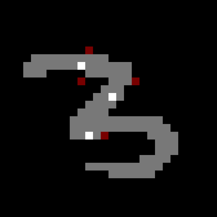
(g) (Misclassified) $k^{\star}=7$

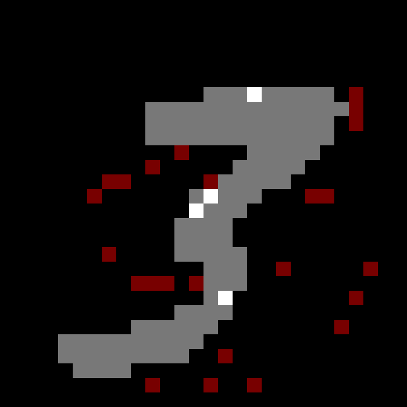
(h) $k^{\star}=28$

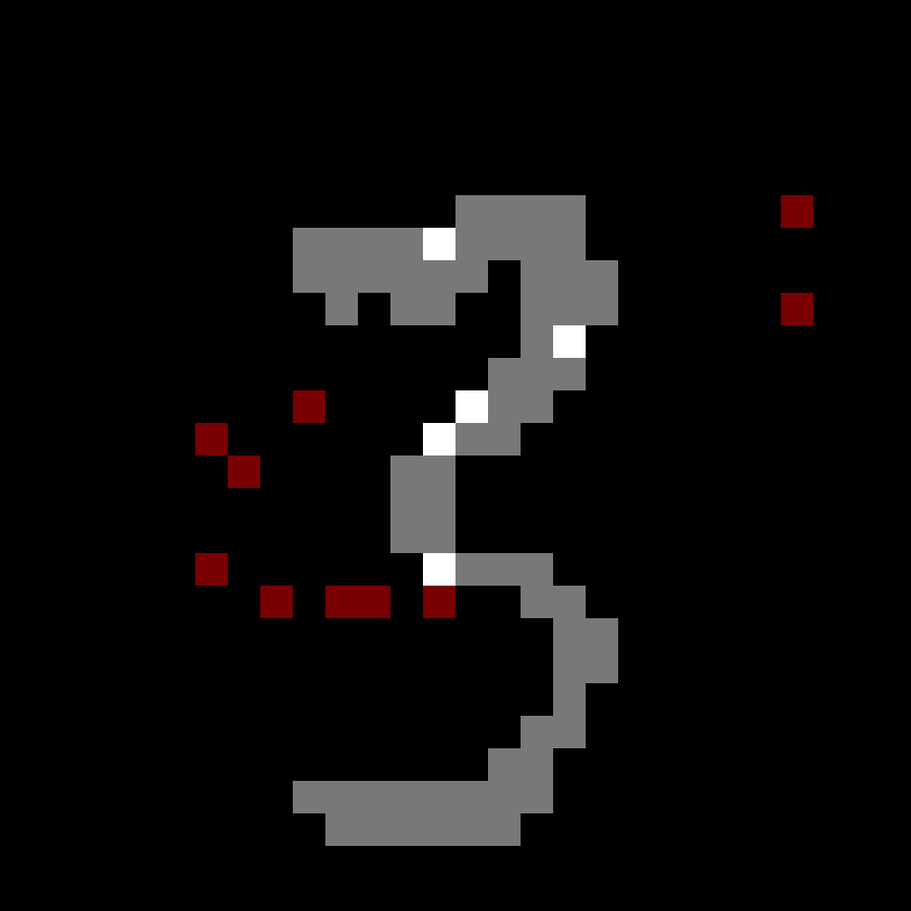
(i) $k^{\star}=15$

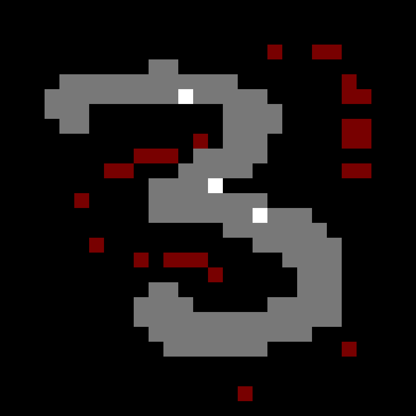
(j) $k^{\star}=30$

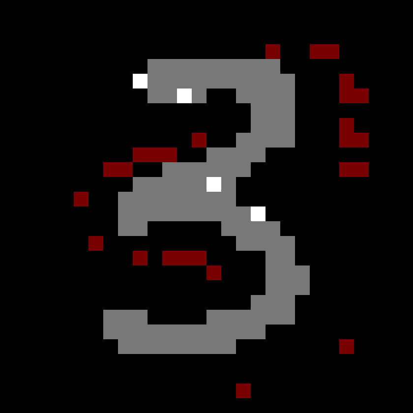
(k) $k^{\star}=30$

(l) $k^{\star}=15$

Figure 13: Examples of Minimum Sufficient Reasons over the MNIST dataset. All images correspond to positive instances for a decision tree of $1486$ leaves that detects the digit $3$. Two instances are misclassified. Light pixels of the original image are depicted in grey, and the light pixels of the original image that are part of the minimum sufficient reason are colored white. Dark pixels that are part of the minimum sufficient reason are colored with red. Individual captions denote the size of the minimum sufficient reasons with $k^{\star}$.

Given the compactness of the deterministic encoding, with  $O(nk+|T|)$ clauses, it is feasible to use it for MNIST instances, for which $n=28\times 28=784$. Tables 2 and 3 exhibit results obtained for this dataset when recognizing digit $1$. Figures 11 and 12 exhibit minimum sufficient reasons for positive and negative instance (respectively) on a decision tree for recognizing the digit $1$. Figures 13 and 14 show examples when recognizing the digit $3$, and finally Figures 15 and 16 exhibit examples when recognizing the digit $9$. Figure 10 shows empirically how time scales linearly with $k^{\star}$, the size of the minimum sufficient reason found.

Probabilistic results

Because of the complexity of the encoding, we test over the synthetic dataset described above in which the dimension is only $5\times 5=25$. Table 4 summarizes the results obtained for this dataset. We emphasize the following observations:

1. Computing probabilistic sufficient reasons through the general probabilistic encoding (i.e., $\delta<1$) is less efficient than computing deterministic ones, even by several orders of magnitude.

2. As the value of $\delta$ approaches one, the size of the minimum $\delta$-SR approaches $k^{\star}$, the size of the minimum sufficient reason for the given instance. On the other hand, as $\delta$ decreases the size of the minimum $\delta$-SR goes to 0. This trade-off implies that $\delta$ can be used to control the size of the obtained explanation.

3. The time per explanation increases significantly as $\delta$ approaches $1$, even though the encoding itself does not get any larger, implying that the resulting $\mathsf{CNF}$ is more challenging. Interestingly enough, for $\delta=1$ the deterministic encoding is very efficient, thus suggesting a discontinuity. It remains a challenging problem to compute $\delta$-SRs for $\delta<1$ in a way that at least matches the efficiency of the case $\delta=1$.

Table 1: Experimental results for the probabilistic encoding over positive instances of tall rectangles. Each datapoint is the average of 3 instances.

$\delta$	Size of smallest explanation	Time	Number of leaves	Accuracy of the tree
0.6	0.0	0.105s	20	0.854
0.7	1.0	0.362s	20	0.854
0.8	2.0	0.669s	20	0.854
0.9	3.0	1.551s	20	0.854
0.95	3.0	1.409s	20	0.854
1.0	3.0	0.032s	20	0.854
0.6	0.0	0.183s	30	0.965
0.7	1.0	0.567s	30	0.965
0.8	1.0	0.578s	30	0.965
0.9	3.67	5.377s	30	0.965
0.95	5.67	12.27s	30	0.965
1.0	6.67	0.037s	30	0.965
0.6	2.0	1.003s	40	0.986
0.7	3.0	2.259s	40	0.986
0.8	4.0	3.507s	40	0.986
0.9	6.0	10.318s	40	0.986
0.95	7.0	16.387s	40	0.986
1.0	10.0	0.046s	40	0.986
0.6	2.67	1.992s	50	1.0
0.7	4.33	6.111s	50	1.0
0.8	5.0	7.216s	50	1.0
0.9	7.0	26.58s	50	1.0
0.95	7.67	33.129s	50	1.0
1.0	8.33	0.044s	50	1.0

Table 2: Experimental results for the deterministic encoding over negative instances of digit $1$ in MNIST. Each datapoint corresponds to the average of 10 instances.

Number of leaves	Size of smallest explanation	Time	Accuracy of the tree
100	3.6	0.17s	0.988
125	3.1	0.141s	0.989
150	3.7	0.196s	0.989
175	4.1	0.216s	0.99
200	4.3	0.255s	0.991
225	3.9	0.269s	0.991
250	4.1	0.304s	0.992
275	4.1	0.334s	0.992
300	4.4	0.329s	0.993
325	4.0	0.292s	0.993
350	4.3	0.327s	0.993
375	4.0	0.283s	0.993
400	5.2	0.337s	0.993
425	6.0	0.346s	0.993
450	6.8	0.495s	0.993
475	6.4	0.401s	0.993
500	5.8	0.497s	0.993

Table 3: Experimental results for the deterministic encoding over positive instances of digit $1$ in MNIST. Each datapoint corresponds to the average of 10 instances.

Number of leaves	Size of smallest explanation	Time	Accuracy of the tree
100	17.0	1.238	0.988
125	17.5	1.077	0.989
150	18.4	1.058	0.989
175	17.9	1.082	0.99
200	19.0	1.001	0.991
225	21.4	1.188	0.991
250	25.0	1.405	0.992
275	23.7	1.183	0.992
300	31.2	1.603	0.993
325	31.3	1.504	0.993
350	28.5	1.365	0.993
375	30.9	1.547	0.993
400	32.1	2.429	0.993
425	34.3	2.188	0.993
450	34.3	2.115	0.993
475	42.5	2.533	0.993
500	43.6	2.614	0.993

Table 4: Experimental results for the randomized encoding, for $\delta=\frac{3}{4}$.

number of leaves	size of smallest explanation	time	accuracy of the tree
15	4	30.44s	0.86
16	1	2.86s	0.84
17	2	6.91s	0.90
18	4	14.59s	0.90
19	3	14.11s	0.88
20	2	6.92s	0.90

Figure 8: Time for computing a minimum sufficient reason $(\delta=1)$ as a function of decision tree size. All datapoints correspond to an average of 10 different instances for decision trees trained to recognize the digit $1$ in the MNIST dataset.

Figure 9: Size of minimum sufficient reasons $(\delta=1)$ as a function of decision tree size. All datapoints correspond to an average of 10 different instances for decision trees trained to recognize the digit $1$ in the MNIST dataset.

Figure 10: Relationship between the size of the Minimum Sufficient Reason and the time it takes to obtain it.

(a) $k^{\star}=49$

(b) $k^{\star}=42$

(c) $k^{\star}=49$

(d) $k^{\star}=49$

(e) $k^{\star}=49$

(f) $k^{\star}=42$

(g) $k^{\star}=49$

(h) $k^{\star}=49$

(i) $k^{\star}=49$

(j) $k^{\star}=49$

(k) $k^{\star}=49$

(l) $k^{\star}=49$

Figure 11: Examples of Minimum Sufficient Reasons over the MNIST dataset. All instances are (correctly predicted) positive instances for a decision tree of $591$ leaves that detects the digit $1$. Light pixels of the original image are depicted in grey, and the light pixels of the original image that are part of the minimum sufficient reason are colored white. Dark pixels that are part of the minimum sufficient reason are colored with red. Individual captions denote the size of the minimum sufficient reasons with $k^{\star}$.

(a) $k^{\star}=5$

(b) $k^{\star}=5$

(c) $k^{\star}=5$

(d) $k^{\star}=5$

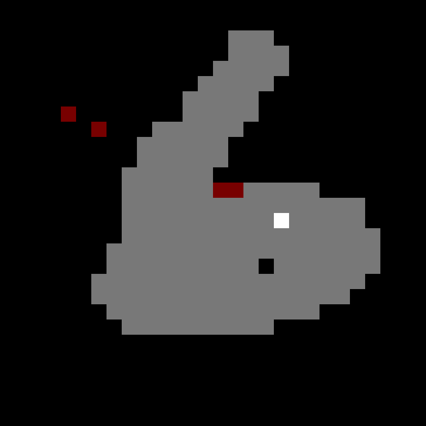
(e) $k^{\star}=5$

(f) $k^{\star}=7$

(g) $k^{\star}=5$

(h) $k^{\star}=5$

(i) $k^{\star}=5$

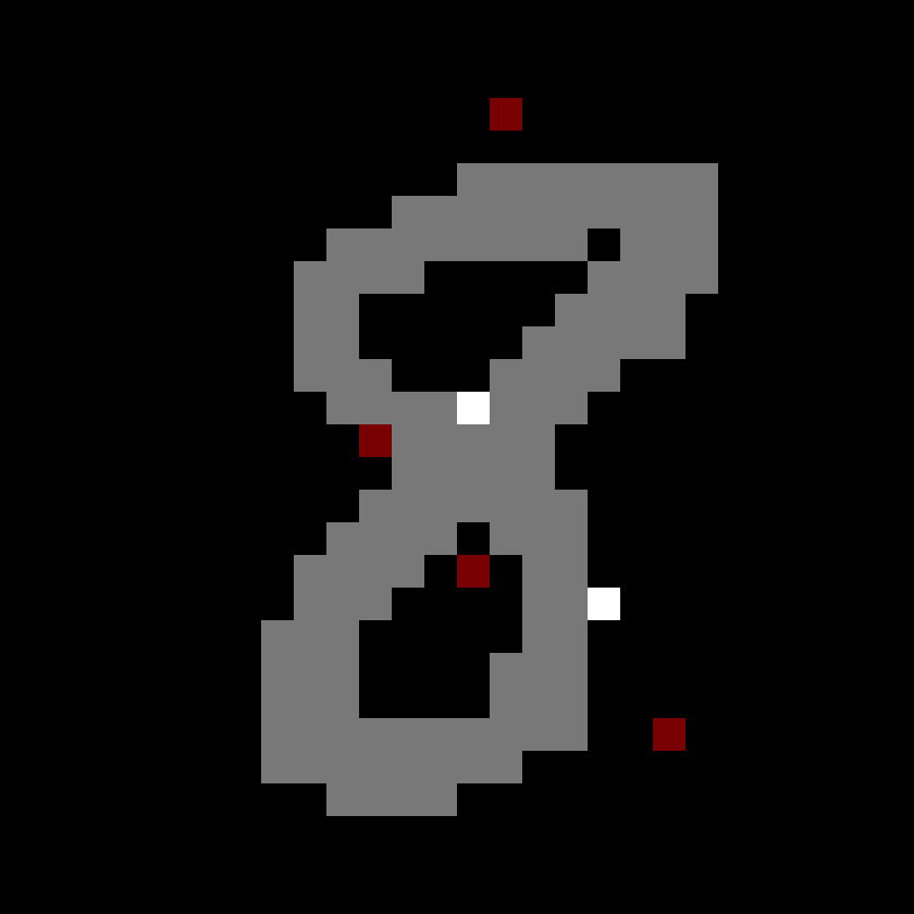
(j) $k^{\star}=6$

(k) $k^{\star}=5$

(l) $k^{\star}=5$

Figure 12: Examples of Minimum Sufficient Reasons over the MNIST dataset. All instances are correctly predicted negative instances for a decision tree of $591$ leaves that detects the digit $1$. Light pixels of the original image are depicted in grey, and the light pixels of the original image that are part of the minimum sufficient reason are colored white. Dark pixels that are part of the minimum sufficient reason are colored with red. Individual captions denote the size of the minimum sufficient reasons with $k^{\star}$.

(a) $k^{\star}=30$

(b) $k^{\star}=19$

(c) $k^{\star}=30$

(d) $k^{\star}=13$

(e) $k^{\star}=17$

(f) (Misclassified) $k^{\star}=9$

(a) $k^{\star}=11$

(b) $k^{\star}=8$

(c) $k^{\star}=11$

(d) $k^{\star}=12$

(e) $k^{\star}=12$

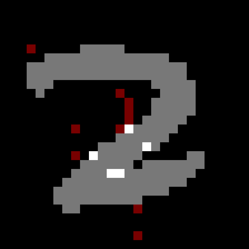
(f) $k^{\star}=15$

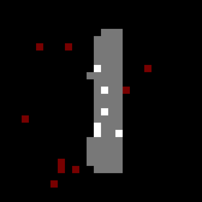
(g) ($k^{\star}=15$

(h) $k^{\star}=11$

(i) $k^{\star}=14$

(j) $k^{\star}=13$

(k) $k^{\star}=11$

(l) $k^{\star}=7$

Figure 14: Examples of Minimum Sufficient Reasons over the MNIST dataset. All images correspond to negative instances for a decision tree of $1486$ leaves that detects the digit $3$ and are classified correctly. Light pixels of the original image are depicted in grey, and the light pixels of the original image that are part of the minimum sufficient reason are colored white. Dark pixels that are part of the minimum sufficient reason are colored with red. Individual captions denote the size of the minimum sufficient reasons with $k^{\star}$.

(a) (Misclassified) $k^{\star}=10$

(b) (Misclassified) $k^{\star}=9$

(c) $k^{\star}=35$

(d) $k^{\star}=18$

(e) $k^{\star}=45$

(f) ($k^{\star}=45$

(g) (Misclassified) $k^{\star}=17$

(h) $k^{\star}=20$

(i) $k^{\star}=45$

(j) $k^{\star}=45$

(k) $k^{\star}=44$

(l) $k^{\star}=45$

Figure 15: Examples of Minimum Sufficient Reasons over the MNIST dataset. All images correspond to positive instances for a decision tree of $1652$ leaves that detects the digit $9$. Three instances are misclassified. Light pixels of the original image are depicted in grey, and the light pixels of the original image that are part of the minimum sufficient reason are colored white. Dark pixels that are part of the minimum sufficient reason are colored with red. Individual captions denote the size of the minimum sufficient reasons with $k^{\star}$.

(a) $k^{\star}=16$

(b) $k^{\star}=8$

(c) $k^{\star}=9$

(d) $k^{\star}=12$

(e) $k^{\star}=5$

(f) ($k^{\star}=12$

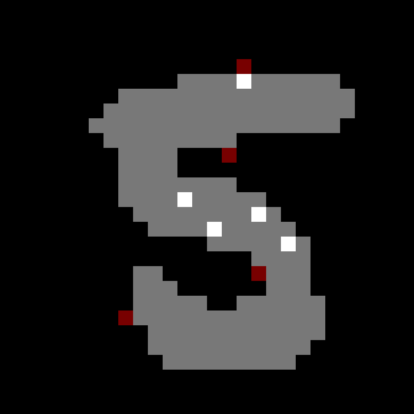
(g) ( $k^{\star}=9$

(h) $k^{\star}=6$

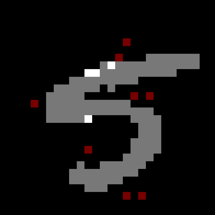
(i) $k^{\star}=12$

(j) $k^{\star}=6$

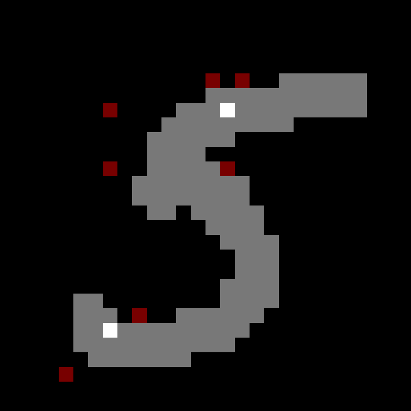
(k) $k^{\star}=9$

(l) $k^{\star}=15$

Figure 16: Examples of Minimum Sufficient Reasons over the MNIST dataset. All images correspond to (correctly classified) negative instances for a decision tree of $1652$ leaves that detects the digit $9$. Light pixels of the original image are depicted in grey, and the light pixels of the original image that are part of the minimum sufficient reason are colored white. Dark pixels that are part of the minimum sufficient reason are colored with red. Individual captions denote the size of the minimum sufficient reasons with $k^{\star}$.

References

- Arenas et al. (2021) M. Arenas, D. Báez, P. Barceló, J. Pérez, and B. Subercaseaux. Foundations of symbolic languages for model interpretability. In M. Ranzato, A. Beygelzimer, Y. Dauphin, P. Liang, and J. W. Vaughan, editors, Advances in Neural Information Processing Systems, volume 34, pages 11690–11701. Curran Associates, Inc., 2021. URL https://proceedings.neurips.cc/paper/2021/file/60cb558c40e4f18479664069d9642d5a-Paper.pdf.
- Arrieta et al. (2020) A. B. Arrieta, N. Díaz-Rodríguez, J. D. Ser, A. Bennetot, S. Tabik, A. Barbado, S. Garcia, S. Gil-Lopez, D. Molina, R. Benjamins, R. Chatila, and F. Herrera. Explainable artificial intelligence (XAI): Concepts, taxonomies, opportunities and challenges toward responsible AI. Information Fusion, 58:82–115, June 2020. doi: 10.1016/j.inffus.2019.12.012. URL https://doi.org/10.1016/j.inffus.2019.12.012.
- Audemard et al. (2021a) G. Audemard, S. Bellart, L. Bounia, F. Koriche, J. Lagniez, and P. Marquis. On the computational intelligibility of boolean classifiers. In M. Bienvenu, G. Lakemeyer, and E. Erdem, editors, Proceedings of the 18th International Conference on Principles of Knowledge Representation and Reasoning, KR 2021, Online event, November 3-12, 2021, pages 74–86, 2021a. doi: 10.24963/kr.2021/8. URL https://doi.org/10.24963/kr.2021/8.
- Audemard et al. (2021b) G. Audemard, S. Bellart, L. Bounia, F. Koriche, J.-M. Lagniez, and P. Marquis. On the explanatory power of decision trees, 2021b. URL https://arxiv.org/abs/2108.05266.
- Barceló et al. (2020) P. Barceló, M. Monet, J. Pérez, and B. Subercaseaux. Model interpretability through the lens of computational complexity. In H. Larochelle, M. Ranzato, R. Hadsell, M. Balcan, and H. Lin, editors, Advances in Neural Information Processing Systems, volume 33, pages 15487–15498. Curran Associates, Inc., 2020. URL https://proceedings.neurips.cc/paper/2020/file/b1adda14824f50ef24ff1c05bb66faf3-Paper.pdf.
- Biere et al. (2009) A. Biere, A. Biere, M. Heule, H. van Maaren, and T. Walsh. Handbook of Satisfiability: Volume 185 Frontiers in Artificial Intelligence and Applications. IOS Press, NLD, 2009. ISBN 1586039296.
- Biere et al. (2020) A. Biere, K. Fazekas, M. Fleury, and M. Heisinger. CaDiCaL, Kissat, Paracooba, Plingeling and Treengeling entering the SAT Competition 2020. In T. Balyo, N. Froleyks, M. Heule, M. Iser, M. Järvisalo, and M. Suda, editors, Proc. of SAT Competition 2020 – Solver and Benchmark Descriptions, volume B-2020-1 of Department of Computer Science Report Series B, pages 51–53. University of Helsinki, 2020.
- Blanc et al. (2021) G. Blanc, J. Lange, and L.-Y. Tan. Provably efficient, succinct, and precise explanations. In A. Beygelzimer, Y. Dauphin, P. Liang, and J. W. Vaughan, editors, Advances in Neural Information Processing Systems, 2021. URL https://openreview.net/forum?id=9UjRw5bqURS.
- Choi et al. (2017) A. Choi, W. Shi, A. Shih, and A. Darwiche. Compiling neural networks into tractable boolean circuits. intelligence, 2017.
- Deng (2012) L. Deng. The mnist database of handwritten digit images for machine learning research. IEEE Signal Processing Magazine, 29(6):141–142, 2012.
- Gilpin et al. (2018) L. H. Gilpin, D. Bau, B. Z. Yuan, A. Bajwa, M. A. Specter, and L. Kagal. Explaining explanations: An overview of interpretability of machine learning. In F. Bonchi, F. J. Provost, T. Eliassi-Rad, W. Wang, C. Cattuto, and R. Ghani, editors, DSAA, pages 80–89, 2018.
- Goldsmith et al. (2005) J. Goldsmith, M. Hagen, and M. Mundhenk. Complexity of DNF and isomorphism of monotone formulas. In Mathematical Foundations of Computer Science 2005, pages 410–421. Springer Berlin Heidelberg, 2005. doi: 10.1007/11549345_36. URL https://doi.org/10.1007/11549345_36.
- Huang et al. (2021) X. Huang, Y. Izza, A. Ignatiev, and J. Marques-Silva. On efficiently explaining graph-based classifiers. In M. Bienvenu, G. Lakemeyer, and E. Erdem, editors, Proceedings of the 18th International Conference on Principles of Knowledge Representation and Reasoning, KR 2021, Online event, November 3-12, 2021, pages 356–367, 2021. doi: 10.24963/kr.2021/34. URL https://doi.org/10.24963/kr.2021/34.
- Ignatiev and Marques-Silva (2021) A. Ignatiev and J. Marques-Silva. SAT-based rigorous explanations for decision lists. In Theory and Applications of Satisfiability Testing – SAT 2021, pages 251–269. Springer International Publishing, 2021. doi: 10.1007/978-3-030-80223-3_18. URL https://doi.org/10.1007/978-3-030-80223-3_18.
- Ignatiev et al. (2022) A. Ignatiev, Y. Izza, P. J. Stuckey, and J. Marques-Silva. Using maxsat for efficient explanations of tree ensembles. In AAAI, 2022.
- Izza et al. (2020a) Y. Izza, A. Ignatiev, and J. Marques-Silva. On explaining decision trees. CoRR, abs/2010.11034, 2020a.
- Izza et al. (2020b) Y. Izza, A. Ignatiev, and J. Marques-Silva. On explaining decision trees, 2020b. URL https://arxiv.org/abs/2010.11034.
- Izza et al. (2021) Y. Izza, A. Ignatiev, N. Narodytska, M. C. Cooper, and J. Marques-Silva. Efficient explanations with relevant sets. ArXiv, abs/2106.00546, 2021.
- Izza et al. (2022) Y. Izza, A. Ignatiev, N. Narodytska, M. C. Cooper, and J. Marques-Silva. Provably precise, succinct and efficient explanations for decision trees, 2022. URL https://arxiv.org/abs/2205.09569.
- Lipton (2018) Z. C. Lipton. The mythos of model interpretability. Queue, 16(3):31–57, 2018.
- Lundberg and Lee (2017) S. M. Lundberg and S.-I. Lee. A unified approach to interpreting model predictions. In NeurIPS, pages 4765–4774, 2017.
- Marques-Silva and Ignatiev (2022) J. Marques-Silva and A. Ignatiev. Delivering trustworthy ai through formal xai. In AAAI, 2022.
- Marques-Silva et al. (2020) J. Marques-Silva, T. Gerspacher, M. C. Cooper, A. Ignatiev, and N. Narodytska. Explaining naive bayes and other linear classifiers with polynomial time and delay. In NeurIPS, 2020.
- Marques-Silva et al. (2021) J. Marques-Silva, T. Gerspacher, M. C. Cooper, A. Ignatiev, and N. Narodytska. Explanations for monotonic classifiers. In ICML, pages 7469–7479, 2021.
- Marques-Silva et al. (2021) J. Marques-Silva, T. Gerspacher, M. C. Cooper, A. Ignatiev, and N. Narodytska. Explanations for monotonic classifiers. In M. Meila and T. Zhang, editors, Proceedings of the 38th International Conference on Machine Learning, volume 139 of Proceedings of Machine Learning Research, pages 7469–7479. PMLR, 18–24 Jul 2021. URL https://proceedings.mlr.press/v139/marques-silva21a.html.
- Pedregosa et al. (2011) F. Pedregosa, G. Varoquaux, A. Gramfort, V. Michel, B. Thirion, O. Grisel, M. Blondel, P. Prettenhofer, R. Weiss, V. Dubourg, J. Vanderplas, A. Passos, D. Cournapeau, M. Brucher, M. Perrot, and E. Duchesnay. Scikit-learn: Machine learning in Python. Journal of Machine Learning Research, 12:2825–2830, 2011.
- Ribeiro et al. (2018) M. T. Ribeiro, S. Singh, and C. Guestrin. Anchors: High-precision model-agnostic explanations. In AAAI, pages 1527–1535, 2018.
- Shih et al. (2018) A. Shih, A. Choi, and A. Darwiche. A symbolic approach to explaining bayesian network classifiers. arXiv preprint arXiv:1805.03364, 2018.
- Sinz (2005) C. Sinz. Towards an optimal CNF encoding of boolean cardinality constraints. In Principles and Practice of Constraint Programming - CP 2005, pages 827–831. Springer Berlin Heidelberg, 2005. doi: 10.1007/11564751_73. URL https://doi.org/10.1007/11564751_73.
- Wäldchen et al. (2021) S. Wäldchen, J. MacDonald, S. Hauch, and G. Kutyniok. The computational complexity of understanding binary classifier decisions. J. Artif. Intell. Res., 70:351–387, 2021.
- Wang et al. (2021) E. Wang, P. Khosravi, and G. V. den Broeck. Probabilistic sufficient explanations. In Z. Zhou, editor, IJCAI, pages 3082–3088, 2021.
- Wegener (2000) I. Wegener. Branching Programs and Binary Decision Diagrams. Society for Industrial and Applied Mathematics, Jan. 2000. doi: 10.1137/1.9780898719789. URL https://doi.org/10.1137/1.9780898719789.
- Wegener (2004) I. Wegener. Bdds–design, analysis, complexity, and applications. Discret. Appl. Math., 138(1-2):229–251, 2004.
- Yan and Procaccia (2021) T. Yan and A. D. Procaccia. If you like shapley then you’ll love the core. In AAAI, pages 5751–5759, 2021.