Spinon confinement in the gapped antiferromagnetic XXZ spin-1/2 chain

Abstract

The infinite Heisenberg XXZ spin-(1/2) chain in the gapped antiferromagnetic regime has two degenerate vacua and kink topological excitations (which are also called spinons) interpolating between these vacua as elementary excitations. Application of an arbitrary weak staggered longitudinal magnetic field $h$ induces a long-range attractive potential between two adjacent spinons leading to their confinement into ’meson’ bound states. Exploiting the integrability of the XXZ model in the deconfined phase $h=0$, we perform perturbative calculations of the energy spectra of the two-spinon bound states in the weak confinement regime at $h\to+0$, using the strength of the staggered magnetic field $h$ as a small parameter. Both transverse and longitudinal dynamical structure factors of the local spin operators are calculated as well in the two-spinon approximation in the weak confinement regime to the leading order in $h$.

October 7, 2022

I Introduction

The notion of confinement plays a significant role in modern physics. This phenomenon occurs if the constituents of compound particles cannot be separated from each other and therefore cannot be observed directly. A famous example is the confinement of quarks in hadrons Narison (2004), whose theoretical description remains a long-standing open problem of Quantum Chromodynamics (QCD).

It is remarkable that confinement of particles finds its realization not only in high-energy physics but also in condensed matter systems. In certain quasi-one-dimensional crystals the confinement of topological kink magnetic excitations becomes experimentally observable and demands for precise theoretical predictions. An example is the compound $\mathrm{Co}\mathrm{Nb}_{2}\mathrm{O}_{6}$ in which kink confinement can be seen e.g. in neutron-scattering experiments Coldea et al. (2010) or high-resolution terahertz spectroscopy Morris et al. (2014). The magnetic structure of this compound Coldea et al. (2010); Fava et al. (2020) can be described by the one-dimensional quantum Ising spin-chain model, which is a paradigmatic model in the theory of quantum phase transitions Sachdev (1999). Kink confinement has been recently also experimentally studied in the quasi-1D antiferromagnetic compounds ${\rm{SrCo_{2}V_{2}O_{8}}}$ Wang et al. (2015); Bera et al. (2017) and ${\rm{BaCo_{2}V_{2}O_{8}}}$ Grenier et al. (2015); Faure et al. (2018); Wang et al. (2019).

The theoretical study of confinement in condense-matter systems was started more than fourty years ago in the pioneering work of McCoy and Wu McCoy and Wu (1978), in which they examined the effect of the external symmetry-breaking magnetic field $h$ on the analytical structure of the two-point function in the Ising Field Theory (IFT) in the ferromagnetic phase. McCoy and Wu demonstrated that the square-root branch cut located at the imaginary axis in the momentum complex plane, which is present in the two-point function in the ordered phase at $h=0$, breaks up into a sequence of poles at any $h>0$. This change in the analytic structure of the two-point function was associated in [McCoy and Wu, 1978] with the confinement transition: fermions, which were free particles in the IFT at $h=0$, attract one-another and form bound states at $h>0$.

It becomes clear later Delfino et al. (1996); Delfino and Mussardo (1998); Mussardo (2011), that the mechanism of confinement discovered by McCoy and Wu in IFT is quite general. It can be realized in many one-dimensional Quantum Field Theories (QFTs) and spin-chain models, which are invariant under a discrete symmetry group and display a continuous order-to-disorder phase transition. If the system has two degenerate vacua $|vac\rangle^{(\mu)}$, $\mu=0,1$ in the ordered phase due to a spontaneous breaking of the $\mathbb{Z}_{2}$-symmetry, the particle sector of the theory should contain kinks $K_{\mu\nu}$, $\mu,\nu=0,1$ that interpolate between these vacua. The application of the symmetry-breaking field, that shifts the energy of the vacuum $|vac\rangle^{(1)}$ to a lower value, lifts the degeneracy between the vacua. As a result, the vacuum $|vac\rangle^{(1)}$ transforms into the true ground state, whereas the state $|vac\rangle^{(0)}$ turns into the unstable false vacuum. The energy difference between the true and false vacuum induces a long-range attractive interaction between kinks, which, in turn, leads to their confinement: isolated kinks do not exist anymore in the system, and the kinks bind into compound particles. In recent decades particular realizations of this scenario in different one-dimensional QFT and spin-chain models have attracted much theoretical interest Shiba (1980); Delfino and Mussardo (1998); Fonseca and Zamolodchikov (2003, 2006); Rutkevich (2005); Delfino and Grinza (2008); Mussardo and Takács (2009); Mussardo (2011); Kormos et al. (2017); Robinson et al. (2019); Lagnese et al. (2020, 2022); Ramos et al. (2020); Lencsés et al. (2022). Note, that due to analogy with QCD, the kinks and two-kink bound states in the confinement regime are often referred to as ‘quarks’ and ‘mesons’, respectively.

In the simplest phenomenological approach to confinement in one-dimension, originating from the work of McCoy and Wu McCoy and Wu (1978), the two kinks are treated as quantum particles with the quadratic dispersion law

$$\omega(p)=m_{0}+\frac{p^{2}}{2m},$$ (1)

moving on the line and attracting one another due to a potential growing linearly with distance and being overall proportional to the external magnetic field $h$. The relative motion of two particles in their center-of-mass frame is described by the Schrödinger equation

$$\left(2m_{0}-\frac{1}{m}\frac{d^{2}}{dx^{2}}+f|x|-E_{n}\right)\psi_{n}(x)=0\,,$$ (2)

where $f\sim h$ is the“string tension”. If the kinks behave as Fermi particles, their wave function must be anti-symmetric, $\psi_{n}(x)=-\psi_{n}(-x)$, and the energy levels of the two-kink bound-states, determined by (2), are given by

$$E_{n}=2m_{0}+z_{n}\,{f^{2/3}}\,{m^{-1{\color[rgb]{0,0,0}/3}}},\quad n=1,2\ldots,$$ (3)

where the numbers $-z_{n}$ are the zeros of the Airy function, $\mathrm{Ai}(-z_{n})=0$. Energy spectra of this form, indicating kink confinement, have been indeed observed Coldea et al. (2010); Grenier et al. (2015); Wang et al. (2015); Bera et al. (2017); Faure et al. (2018) in quasi-1D quantum magnets close to the band minima at symmetry points of the Brillouin zone.

Several numerical techniques applied to microscopic model Hamiltonians (e.g. the truncated conformal space approach Lencsés and Takács (2014, 2015), a tangent-space method for matrix product states, the density matrix renormalization group algorithm Bera et al. (2017)) have been used to obtain the meson (two-kink bound state) spectra in the whole Brillouin zone. Nowadays, the unprecedented increase of accuracy of such numerical techniques allows one in some cases to directly compare the experimental data with numerical results. Nevertheless, it is highly desirable to complement the direct numerical studies with analytical calculations of the meson energy spectra in one-dimensional QFTs and spin-chain models for at least two reasons. First, consistent first-principles analytic calculations allow one to put the conclusions of the numerical analysis on the firm ground. Second, analytic calculations are absolutely necessary for a deep and qualitative understanding of the underlying physics.

Although the confinement caused by the mechanism outlined above does not realize in exactly solvable models, it is quite common in non-integrable deformations of integrable models induced by the discrete-symmetry breaking field $h$. Due to the absence of exact solutions, it is natural to restrict the analysis to the weak confinement regime corresponding to a small symmetry breaking field, and to employ some perturbation theory using $h$ as a small parameter. Two perturbative techniques nicely complementing one another have been used in the literature.

The first more rigorous and consistent (but technically demanding) approach is based on combining the Bethe-Salpeter equation Fonseca and Zamolodchikov (2003, 2006) with a modified form factor expansion Delfino et al. (1996); Rutkevich (2009, 2017). Up to now, this technique has been used for the calculation of meson energy spectra only in two models of statistical mechanics : in the IFT Fonseca and Zamolodchikov (2003, 2006); Rutkevich (2005, 2009), and in the quantum Ising spin chain Rutkevich (2008). Both models have a very specific property, which was substantially exploited in derivation of the Bethe-Salpeter equations Fonseca and Zamolodchikov (2003); Rutkevich (2008): the kink elementary excitations in the deconfined phase of these models do not interact with each other, but behave as free Fermi-particles. This property does not hold in other integrable models, such as the Potts and sine-Gordon QFTs, XXZ spin chain, etc. In these models particles strongly interact at small distances already in the deconfined phase at $h=0$. This short-range interaction is encoded in the non-trivial factorizable scattering matrix, which is the key characteristic of the integrable model. An extension of the systematic perturbative approach exploiting the Bethe-Salpeter equation to confinement in such systems was identified by Fonseca and Zamolodchikov Fonseca and Zamolodchikov (2006) in 2006 as an important open problem.

The second perturbative technique is not so rigorous, but, instead, rather heuristic and intuitive. Its main advantages are the simplicity of calculations and transparency of physical interpretation. In this approach, the two kinks forming a meson are treated as classical particles, which move along the line and attract one another with a constant force. The kinetic energies of these particles are given by the dispersion relation of kinks. The energy spectrum of their bound states is determined in this technique by the semiclassical (or canonical) quantization of the classical kink dynamics. To leading order in $h$, the meson energy spectra obtained by the two aforementioned methods, coincide both for the IFT, and for the Ising spin chain.

One more important advantage of the second (heuristic) method is that it can be applied, after a proper modification, to models, in which kinks are not free, but interact with each other already in the deconfined phase at $h=0$. This modification was introduced in paper [Rutkevich, 2010], in which the meson mass spectrum in the Potts field theory was studied. It was shown there, that the strong short-range interaction between kinks in the deconfined phase of this model can be accounted for by the semiclassical Bohr-Sommerfeld quantization condition by adding the two-kink scattering phase to its left-hand side. As a result, the semiclassical meson mass spectrum determined by the modified Bohr-Sommerfeld rule carries information about the non-trivial kink-kink scattering in the deconfined phase. By means of this improved semiclassical technique, the meson energy spectra were later calculated in several models exhibiting confinement, including the XXZ spin chain in a staggered magnetic field Rutkevich (2018), the XXZ spin ladder Lagnese et al. (2022), the transverse-field Ising ladder Ramos et al. (2020), and the thermally deformed tricritical Ising model Lencsés et al. (2022).

In this work, we continue our study of the kink confinement in the gapped antiferromagnetic XXZ spin chain in a weak staggered magnetic field, initiated in Rutkevich (2018). The Hamiltonian of the model is given by

$$\mathcal{H}(h) =-\frac{J}{2}\sum_{j=-\infty}^{\infty}\!\!\left(\sigma_{j}^{x}\sigma_{j+1}^{x}+\sigma_{j}^{y}\sigma_{j+1}^{y}+\Delta\,\sigma_{j}^{z}\sigma_{j+1}^{z}\right)$$

$$-h\sum_{j=-\infty}^{\infty}(-1)^{j}\sigma_{j}^{z}.$$ (4)

Here the index $j$ enumerates the spin-chain sites, $\sigma_{j}^{\mathfrak{a}}$ are the Pauli matrices, $\mathfrak{a}=x,y,z$, $J>0$ is the coupling constant, $\Delta<-1$ is the anisotropy parameter, $h$ is the strength of the staggered magnetic field. Model (4) has been used by Bera et al. Bera et al. (2017) for the interpretation of their neutron scattering investigations of the magnetic excitations in the quasi-1D antiferromagnetic compound ${\rm{SrCo_{2}V_{2}O_{8}}}$. The effective staggered field accounts in the mean-field approximation for the weak inter-chain interaction in a three-dimensional (3D) array of parallel spin chains in the 3D-ordered phase of such compounds, as it was suggested by Shiba Shiba (1980).

Exploiting the integrability of model (4) in the deconfined phase at $h=0$, we perform two alternative perturbative calculations of the meson energy spectra in the weak confinement regime $h\to+0$ to the first order in the small parameter $h$. First, we present the details of the calculation announced previously Rutkevich (2018), which employs the non-rigorous heuristic procedure outlined above. Then, we derive the Bethe-Salpeter equation for model (4) in the two-kink approximation. From the perturbative solution of this equation, we calculate in a systematic fashion the meson energy spectra, and justify previously obtained results. Furthermore, we derive from the perturbative solutions of the Bethe-Salpeter equation the explicit formulas for the two-kink contribution to the Dynamical Structure Factors (DSF) of the local spin operators for model (4) at zero temperature in the weak confinement regime.

The paper is structured in the following way. In Sections II and III, we recall some well-known properties of the XXZ spin-1/2 infinite chain in the gapped antiferromagnetic phase at zero magnetic field. Section II contains information about some basic properties of the low-energy excitations in this model and the structure of their Hilbert space. Section III is devoted to the DSF of local spin operators in model (4) at $h=0$. By means of a straightforward unified calculation procedure, we derive new explicit formulas for the transverse and longitudinal DSF in the deconfined phase in the two-kink approximation. Starting from Sections IV, we proceed to the analysis of the confinement in model (4) induced by a weak staggered magnetic field $h>0$. In Section IV we classify the meson bound states in the weak confinement regime, and describe the heuristic calculation of their energy spectra. The Bethe-Salpeter equation for model (4) is derived in Section V. The perturbative solution of this equation in several asymptotical regimes is given in Section VI. Using the results of this asymptotic analysis, we derive the initial terms of the small-$h$ expansion for the meson energy spectra, and justify the results of the previous non-rigorous heuristic calculations of these spectra. Section VII contains the calculation of the two-kink contribution to the transverse and longitudinal DSF in the confinement regime in the leading order in the staggered field $h$. Concluding remarks are presented in Section VIII. Finally, some technical details are relegated to four Appendixes.

II Infinite XXZ spin chain at zero magnetic field

In this section, we remind some well-known properties of the XXZ spin-1/2 chain (4) at zero staggered magnetic field. At $h=0$, the Hamiltonian (4) reduces to the form $H=\mathcal{H}(0)$:

$${H}=-\frac{J}{2}\sum_{j=-\infty}^{\infty}\!\!\left(\sigma_{j}^{x}\sigma_{j+1}^{x}+\sigma_{j}^{y}\sigma_{j+1}^{y}+{\Delta}\,\sigma_{j}^{z}\sigma_{j+1}^{z}\right).$$ (5)

Three phases are realized in the infinite spin chain (5) at zero temperature in different regions of the anisotropy parameter $\Delta$: the ferromagnetic phase at $\Delta>1$, the critical phase (spin-fluid, Luttinger liquid) at $-1<\Delta<1$, and the gapped (massive) antiferromagnetic phase at $\Delta<-1$. Only the gapped antiferromagnetic phase will be considered in this paper. We shall use the standard parametrisation for the anisotropy parameter $\Delta<-1$:

$${\Delta}=({q}+{q}^{-1})/2=-\cosh\eta,$$ (6)

$$q=-\exp(-\eta)\in(-1,0),\quad\eta>0.$$ (7)

The Hamiltonian (5) commutes with the $z$-projection of the total spin

$$S^{z}=\frac{1}{2}\sum_{j=-\infty}^{\infty}\sigma_{j}^{z}.$$ (8)

For short, the operator $S^{z}$ will be called the ”total spin” in the sequel. The Hamiltonian (5) commutes as well with the unitary operator $U=\otimes_{j\in\mathbb{Z}}\,\sigma_{j}^{x},$ and with the translation operator by one chain site ${T}_{1}$, that acts on the Pauli matrices as

$${T}_{1}^{-1}\sigma_{j}^{\mathfrak{a}}{T}_{1}=\sigma_{j+1}^{\mathfrak{a}}.$$ (9)

Note, that

$$U\sigma_{j}^{y,z}U^{-1}=-\sigma_{j}^{y,z},\quad U\sigma_{j}^{x}U^{-1}=\sigma_{j}^{x}.$$ (10)

It is also useful to introduce the modified translation operator $\widetilde{T}_{1}=T_{1}U$, which, of course, commutes with the Hamiltonian (5) as well. Its action on the Pauli matrices can be read from equations (9), (10):

$$\widetilde{T}_{1}^{-1}\sigma_{j}^{y,z}\widetilde{T}_{1}=-\sigma_{j+1}^{y,z},\quad\widetilde{T}_{1}^{-1}\sigma_{j}^{x}\widetilde{T}_{1}=\sigma_{j+1}^{x}.$$ (11)

The structure of the ground-states and low-energy excitations of the infinite chain (5) in the gapped antiferromagnetic phase is well known Jimbo and Miwa (1995). Since this structure is qualitatively the same for all $\Delta<-1$, it can be well understood by considering the Ising limit case $\Delta\to-\infty$, where the Hamiltonian simplifies drastically. In this limit, it is convenient to rescale the Hamiltonian (5) and to add to it a suitable (infinite in the thermodynamic limit) constant:

$${H}_{I}(\varepsilon)\equiv\frac{{H}}{J|\Delta|}+Const={H}_{I}^{(0)}+\varepsilon V,$$ (12)

where $\varepsilon=|\Delta|^{-1}$ is a small parameter, and

$${H}_{I}^{(0)}=\frac{1}{2}\sum_{j=-\infty}^{\infty}(\sigma_{j}^{z}\sigma_{j+1}^{z}+1),$$ (13)

$$V=\sum_{j=-\infty}^{\infty}(\sigma_{j}^{+}\sigma_{j+1}^{-}+\sigma_{j}^{-}\sigma_{j+1}^{+}),$$

with $\sigma_{j}^{\pm}=\frac{1}{2}(\sigma_{j}^{x}\pm i\sigma_{j}^{y})$.

The model (5) considered on a finite chain is solvable by the Bethe Ansatz method Orbach (1958), see also Takahashi (2005); Zvyagin (2010); Dugave et al. (2015) for further references. In the thermodynamic limit, the Hilbert space $\mathcal{L}$ of low-energy states of model (5) can be represented as the direct sum of four subspaces

$$\mathcal{L}=\mathcal{L}_{00}\oplus\mathcal{L}_{11}\oplus\mathcal{L}_{01}\oplus\mathcal{L}_{10}.$$ (14)

The subspaces $\mathcal{L}_{\mu\nu}$ will be called the topological sectors. The subspaces $\mathcal{L}_{00}\oplus\mathcal{L}_{11}$ and $\mathcal{L}_{01}\oplus\mathcal{L}_{10}$ represent the topologically neutral and topologically charged sectors, respectively. Each subspace $\mathcal{L}_{\mu\nu}$, in turn, can be decomposed into the sum of $n$-particle subspaces, with $n$ even for the neutral topological sectors, and $n$ odd for the charged topological sectors:

$$\mathcal{L}_{00}=\oplus_{m=0}^{\infty}\,\mathcal{L}_{00}^{(2m)},\quad\mathcal{L}_{11}=\oplus_{m=0}^{\infty}\,\mathcal{L}_{11}^{(2m)},$$ (15)

$$\mathcal{L}_{01}=\oplus_{m=0}^{\infty}\,\mathcal{L}_{01}^{(2m+1)},\quad\mathcal{L}_{10}=\oplus_{m=0}^{\infty}\,\mathcal{L}_{10}^{(2m+1)}.$$ (16)

Two vacuum subspaces $\mathcal{L}_{00}^{(0)}$, $\mathcal{L}_{11}^{(0)}$ are one-dimensional, while all other subspaces $\mathcal{L}_{\mu\nu}^{(n)}$, $n>0$ have infinite dimensions.

II.1 Vacuum sector

There are two degenerate ground states $|vac\rangle^{(\mu)}$, $\mu=0,1$, showing a Néel-type order,

$$\phantom{.}{}^{(1)}\langle vac|\sigma_{j}^{z}|vac\rangle^{(1)}=(-1)^{j}\bar{\sigma},$$ (17)

$$\phantom{.}{}^{(0)}\langle vac|\sigma_{j}^{z}|vac\rangle^{(0)}=-(-1)^{j}\bar{\sigma}.$$ (18)

with the staggered spontaneous magnetization Baxter (1973, 1976); Izergin et al. (1999)

$$\bar{\sigma}(\eta)=\prod_{n=1}^{\infty}\left(\frac{1-e^{-2n\eta}}{1+e^{-2n\eta}}\right)^{2}.$$ (19)

In the Ising limit $\eta\to\infty$ these ground states become the pure Néel states:

$$\lim_{\eta\to\infty}|vac\rangle^{(1)}=|0\rangle^{(1)}:\quad\ldots\downarrow{\color[rgb]{0,0,1}\ \underline{\stackrel{{\scriptstyle 0}}{{\uparrow}}}}\stackrel{{\scriptstyle 1}}{{\downarrow}}\stackrel{{\scriptstyle 2}}{{\uparrow}}\downarrow\ldots,$$ (20a)

$$\lim_{\eta\to\infty}|vac\rangle^{(0)}=|0\rangle^{(0)}:\quad\ldots\uparrow{\color[rgb]{0,0,1}\underline{\stackrel{{\scriptstyle 0}}{{\downarrow}}}}\stackrel{{\scriptstyle 1}}{{\uparrow}}\stackrel{{\scriptstyle 2}}{{\downarrow}}\uparrow\ldots,$$ (20b)

and $\bar{\sigma}(\eta)\to 1$.

The Hamiltonian symmetries corresponding to the operators $T_{1}$ and $U$ are spontaneously broken in the antiferromagnetic phase,

$$T_{1}|vac\rangle^{(1)}=|vac\rangle^{(0)},\quad T_{1}|vac\rangle^{(0)}=|vac\rangle^{(1)},$$ (21)

$$U|vac\rangle^{(1)}=|vac\rangle^{(0)},\quad U|vac\rangle^{(0)}=|vac\rangle^{(1)}.$$ (22)

On the other hand, the antiferromagnetic vacua $|vac\rangle^{(\mu)}$ are invariant with the respect to the modified translation operator $\widetilde{T}_{1}$,

$$\widetilde{T}_{1}|vac\rangle^{(\mu)}=|vac\rangle^{(\mu)},\;\;{\rm with}\;\;\mu=0,1.$$ (23)

The ground-state energy $E_{N}(\Delta)$ of the periodic chain having $N$ sites increases linearly with $N$ in the thermodynamic limit:

$$\lim_{N\to\infty}\frac{E_{N}(\Delta)}{N}=\frac{J}{2}C(\Delta).$$ (24)

The ground-state energy per lattice site defined by the above equation is explicitly known due to Yang and Yang Yang and Yang (1966a, b). The ground state energy $E_{N}(\Delta)$ diverges in the thermodynamic limit $N\to\infty$. In order to get rid of it, it is convenient to redefine the Hamiltonian (5) by adding an appropriate constant term

$${H}_{1}=-\frac{J}{2}\sum_{j=-\infty}^{\infty}\!\!\Big{(}\sigma_{j}^{x}\sigma_{j+1}^{x}+\sigma_{j}^{y}\sigma_{j+1}^{y}+{\Delta}\,\sigma_{j}^{z}\sigma_{j+1}^{z}+C(\Delta)\Big{)},$$ (25)

such that

$${H}_{1}|vac\rangle^{(\mu)}=0,$$ (26)

with $\mu=0,1$.

II.2 One-kink sector

The elementary excitations are topologically charged, represented Jimbo and Miwa (1995) by the kinks $|K_{\mu\nu}({p})\rangle_{s}$ interpolating between the vacua $\mu$ and $\nu$, and characterized by the quasimomentum ${p}\in\mathbb{R}$, and by the $z$-projection of the spin $s=\pm 1/2$,

$${H}_{1}|K_{\mu\nu}({p})\rangle_{s}=\omega(p)\,|K_{\mu\nu}({p})\rangle_{s},$$ (27a)

$$\widetilde{T}_{1}|K_{\mu\nu}({p})\rangle_{s}=e^{i{p}}\,|K_{\mu\nu}({p})\rangle_{-s},$$ (27b)

$$S^{z}|K_{\mu\nu}({p})\rangle_{s}=s\,|K_{\mu\nu}({p})\rangle_{s}~{}.$$ (27c)

They also satisfy the symmetry properties:

$${T}_{1}|K_{\mu\nu}({p})\rangle_{s}=e^{i{p}}\,|K_{\nu\mu}({p})\rangle_{s},$$ (28a)

$$U|K_{\mu\nu}({p})\rangle_{s}=|K_{\nu\mu}({p})\rangle_{-s},$$ (28b)

$$|K_{\mu\nu}({p+\pi})\rangle_{s}=\varkappa(\mu,s)\,|K_{\mu\nu}({p})\rangle_{s},$$ (28c)

where

$$\varkappa(0,1/2)=\varkappa(1,-1/2)=1,$$ (29)

$$\varkappa(1,1/2)=\varkappa(0,-1/2)=-1.$$

The quantum number $s=\pm 1/2$ will be called “the spin” for short. Since the kinks carry spin $\pm 1/2$, they are also often called “spinons”. We shall use both terms as synonyms. The spinon dispersion law was found by Johnson, Krinsky, and McCoy Johnson et al. (1973),

$$\omega({p},\eta)=I\,\sqrt{1-k^{2}\cos^{2}{p}},$$ (30)

where

$$I=\frac{2JK}{\pi}\sinh\eta,$$ (31)

and $K$ [$K^{\prime}$] is the complete elliptic integral of modulus $k$ [$k^{\prime}=\sqrt{1-k^{2}}$] such that

$$\frac{K^{\prime}}{K}=\frac{\eta}{\pi}.$$ (32)

Note, that the spinon dispersion law (30) coincides up to a numerical factor and re-parametrization with the kink dispersion law Rutkevich (2008)

$$\omega_{{I\!s}}({p},h_{x})=2(1+h_{x})\,\sqrt{1-\frac{4h_{x}}{(1+h_{x})^{2}}\cos^{2}(p/2)},$$ (33)

in the ferromagnetic Ising spin chain in the transverse magnetic field $h_{x}$. The latter model is defined by the Hamiltonian

$${H}_{{I\!s}}=-\sum_{j=-\infty}^{\infty}(\sigma_{j}^{z}\sigma_{j+1}^{z}+h_{x}\sigma_{j}^{x}).$$ (34)

The ferromagnetic phase in this well-studied integrable model is realized at $|h_{x}|<1$.

The dispersion law (30) can be parametrized in terms of the Jacobi elliptic functions of modulus $k$:

$${p}(\alpha)=-\frac{\pi}{2}+\mathrm{am}\,\left(\frac{2K\alpha}{\pi},k\right),$$ (35)

$$\omega(\alpha)=I\,\mathrm{dn}\,\left(\frac{2K\alpha}{\pi},k\right)=J\sinh\eta\,\,\frac{dp(\alpha)}{d\alpha},$$ (36)

where $\alpha$ is the rapidity variable .

The space $\mathcal{L}^{(1)}$ of one-kink states is the sum of two subspaces $\mathcal{L}^{(1)}=\mathcal{L}_{01}^{(1)}\oplus\mathcal{L}_{10}^{(1)}$, which are spanned by basis vectors $|K_{01}({p})\rangle_{s}$ and $|K_{10}({p})\rangle_{s}$, respectively. These basis vectors are normalised by the condition

$$\phantom{.}_{s}\langle K_{\nu\mu}(p)|K_{\mu^{\prime}\nu^{\prime}}(p^{\prime})\rangle_{s^{\prime}}=\pi\delta_{\mu\mu^{\prime}}\delta_{\nu\nu^{\prime}}\delta_{ss^{\prime}}\delta(p-p^{\prime}),$$ (37)

for $p,p^{\prime}\in[0,\pi)$.

Commonly used are also the kink states $|\mathcal{K}_{\mu\nu}(\xi)\rangle_{s}$ parametrised by the complex spectral parameter $\xi(\alpha)=-ie^{i\alpha}$. These states differ from $|K_{\mu\nu}(p)\rangle_{s}$ by the numerical factor $\sqrt{p^{\prime}(\alpha})$:

$$|\mathcal{K}_{\mu\nu}(\xi)\rangle_{s}=\sqrt{\frac{\omega(p)}{J\sinh\eta}}\,\,|K_{\mu\nu}(p)\rangle_{s}.$$ (38)

Note, that a different notation $|\xi\rangle_{\epsilon;(i)}$ has been widely used Jimbo and Miwa (1995) for the one-kink states $|\mathcal{K}_{\mu\nu}(\xi)\rangle_{s}$, with $\epsilon=\mathrm{sign}\,s$, and $i=\nu$.

The completeness relations for the projection operators on the subspaces $\mathcal{L}_{01}^{(1)}$ and $\mathcal{L}_{10}^{(1)}$ read:

$$\mathcal{P}_{01}^{(1)}=\sum_{s=\pm 1/2}\int_{0}^{\pi}\frac{dp}{\pi}|K_{01}(p)\rangle_{s}\phantom{.}{}_{s}\langle K_{10}(p)|=$$ (39a)

$$\sum_{s=\pm 1/2}\int_{0}^{\pi}\frac{d\alpha}{\pi}|\mathcal{K}_{01}[\xi(\alpha)]\rangle_{s}\phantom{.}{}_{s}\langle\mathcal{K}_{10}[\xi(\alpha)]|,$$

$$\mathcal{P}_{10}^{(1)}=\sum_{s=\pm 1/2}\int_{0}^{\pi}\frac{dp}{\pi}|K_{10}(p)\rangle_{s}\phantom{.}{}_{s}\langle K_{01}(p)|=$$ (39b)

$$\sum_{s=\pm 1/2}\int_{0}^{\pi}\frac{d\alpha}{\pi}|\mathcal{K}_{10}[\xi(\alpha)]\rangle_{s}\phantom{.}{}_{s}\langle\mathcal{K}_{01}[\xi(\alpha)]|.$$

It is instructive to describe the kink states $|K_{\mu\nu}({p})\rangle_{s}$ explicitly in the Ising limit $\eta\gg 1$ by means of the Rayleigh-Schrödinger perturbation theory in the small parameter $\varepsilon=1/\cosh\eta$ for the Hamiltonian (12). To this end, one can first consider the localized kink states $|\mathbf{K}_{\mu\nu}(j)\rangle$, which interpolate between vacua $|0\rangle^{(\mu)}$ to the left, and $|0\rangle^{(\nu)}$ to the right of the bond $(j,j+1)$:

$$|\mathbf{K}_{10}(j)\rangle:\quad\ldots\downarrow{\color[rgb]{0,0,1}\ \underline{\stackrel{{\scriptstyle 0}}{{\uparrow}}}}\stackrel{{\scriptstyle 1}}{{\downarrow}}\uparrow\downarrow\ldots\downarrow{\color[rgb]{0.2,0.54,0.2}{\stackrel{{\scriptstyle j}}{{\uparrow}}}}\,\,{\color[rgb]{1,0,0}\mid}{\color[rgb]{0.2,0.54,0.2}{\stackrel{{\scriptstyle j+1}}{{\uparrow}}}}\downarrow\uparrow\ldots,\quad\text{at even }j,$$

$$|\mathbf{K}_{10}(j)\rangle:\quad\ldots\downarrow{\color[rgb]{0,0,1}\ \underline{\stackrel{{\scriptstyle 0}}{{\uparrow}}}}\stackrel{{\scriptstyle 1}}{{\downarrow}}\uparrow\downarrow\ldots\uparrow{\color[rgb]{0.2,0.54,0.2}{\stackrel{{\scriptstyle j}}{{\downarrow}}}}\,\,{\color[rgb]{1,0,0}\mid}{\color[rgb]{0.2,0.54,0.2}{\stackrel{{\scriptstyle j+1}}{{\downarrow}}}}\uparrow\downarrow\ldots,\quad\text{at odd }j,$$

$$|\mathbf{K}_{01}(j)\rangle:\quad\ldots\uparrow{\color[rgb]{0,0,1}\underline{\stackrel{{\scriptstyle 0}}{{\downarrow}}}}\stackrel{{\scriptstyle 1}}{{\uparrow}}\downarrow\uparrow\ldots\downarrow{\color[rgb]{0.2,0.54,0.2}{\stackrel{{\scriptstyle j}}{{\uparrow}}}}\,\,{\color[rgb]{1,0,0}\mid}{\color[rgb]{0.2,0.54,0.2}{\stackrel{{\scriptstyle j+1}}{{\uparrow}}}}\downarrow\uparrow\ldots,\quad\text{at odd }j,$$

$$|\mathbf{K}_{01}(j)\rangle:\quad\ldots\uparrow{\color[rgb]{0,0,1}\underline{\stackrel{{\scriptstyle 0}}{{\downarrow}}}}\stackrel{{\scriptstyle 1}}{{\uparrow}}\downarrow\uparrow\ldots\uparrow{\color[rgb]{0.2,0.54,0.2}{\stackrel{{\scriptstyle j}}{{\downarrow}}}}\,\,{\color[rgb]{1,0,0}\mid}{\color[rgb]{0.2,0.54,0.2}{\stackrel{{\scriptstyle j+1}}{{\downarrow}}}}\uparrow\downarrow\ldots,\quad\text{at even }j.$$

These states are the eigenvectors of the zero-order Hamiltonian ${H}_{I}^{(0)}$, which are characterized by the same (unit) eigenvalue:

$${H}_{I}^{(0)}|\mathbf{K}_{\mu\nu}(j)\rangle=|\mathbf{K}_{\mu\nu}(j)\rangle.$$ (40)

The localized kink states $|\mathbf{K}_{\mu\nu}(j)\rangle$ are normalized by the condition

$$\langle\mathbf{K}_{\nu\mu}(j)|\mathbf{K}_{\mu^{\prime}\nu^{\prime}}(j^{\prime})\rangle=\delta_{\mu\mu^{\prime}}\delta_{\nu\nu^{\prime}}\delta_{jj^{\prime}}.$$ (41)

Their transformation properties under the action of the symmetry operators read:

$${T}_{1}|\mathbf{K}_{\mu\nu}(j)\rangle=|\mathbf{K}_{\nu\mu}(j-1)\rangle,$$

$$U|\mathbf{K}_{\mu\nu}(j)\rangle=|\mathbf{K}_{\nu\mu}(j)\rangle,$$

$$\widetilde{T}_{1}|\mathbf{K}_{\mu\nu}(j)\rangle=|\mathbf{K}_{\mu\nu}(j-1)\rangle.$$

The degeneracy in the excitation energy is removed in the first oder in $\varepsilon$:

$${H}_{I}(\varepsilon)|K_{\mu\nu}^{I}(p)\rangle_{s}=[1-2\varepsilon\cos(2p)]|K_{\mu\nu}^{I}(p)\rangle_{s}+O(\varepsilon^{2}).$$ (42)

The first-oder perturbative result for the kink energy in this equation recovers two initial terms in the Taylor expansion in $\varepsilon$ of the exact kink energy (30):

$$\frac{\omega(p)}{J|\Delta|}=1-2\varepsilon\cos(2p)+\varepsilon^{2}\,\left[\frac{3}{2}-\cos(4{p})\right]+O(\varepsilon^{3}).$$ (43)

The first-order eigenstates $|K_{\mu\nu}^{I}(p)\rangle_{s}$ in (42) denote the kink Bloch states in the Ising limit:

$$|K_{10}^{I}(p)\rangle_{1/2}=\sum_{m=-\infty}^{\infty}e^{i\,(2m+1)p}|\mathbf{K}_{10}(2m)\rangle,$$ (44a)

$$|{K}_{01}^{I}(p)\rangle_{1/2}=\sum_{m=-\infty}^{\infty}e^{2i\,mp}|\mathbf{K}_{01}(2m-1)\rangle,$$ (44b)

$$|K_{10}^{I}(p)\rangle_{-1/2}=\sum_{m=-\infty}^{\infty}e^{2i\,mp}|\mathbf{K}_{10}(2m-1)\rangle,$$ (44c)

$$|K_{01}^{I}(p)\rangle_{-1/2}=\sum_{m=-\infty}^{\infty}e^{i\,(2m+1)p}|\mathbf{K}_{01}(2m)\rangle.$$ (44d)

Due to (41), the kink Bloch states (44) satisfy at $p,p^{\prime}\in[0,\pi)$ the normalisation condition

$$\phantom{.}{}_{s}\langle K_{\nu\mu}^{I}(p)|K_{\mu^{\prime}\nu^{\prime}}^{I}(p^{\prime})\rangle_{s^{\prime}}=\pi\delta_{\mu\mu^{\prime}}\delta_{ss^{\prime}}\delta(p-p^{\prime}).$$ (45)

These states satisfy also equations (27b), (27c), (28), and (39). All these properties indicate that the states $|K_{\mu\nu}^{I}(p)\rangle_{s}$ indeed represent the Ising limit of the one-kink topological excitations $|K_{\mu\nu}(p)\rangle_{s}$ in the infinite antiferromagnetic XXZ spin chain (5):

$$\lim_{\varepsilon\to 0}|K_{\mu\nu}(p)\rangle_{s}=|K_{\mu\nu}^{I}(p)\rangle_{s}.$$ (46)

Note, that equation (35) describing the relation between the momentum and rapidity variables reduces in the Ising limit $\eta\to\infty$ to the simple linear dependence:

$$p(\alpha)=-\frac{\pi}{2}+\alpha+O(e^{-\eta}).$$ (47)

The opposite limit $\eta\ll 1$ corresponds to the scaling regime. In this limit, the kink dispersion law (30) at small momenta $p$ takes the relativistic form:

$$\omega(p,\eta)=Ik\sqrt{m^{2}+p^{2}}\left[1+O\left(\frac{p^{4}}{m^{2}+p^{2}}\right)\right],$$ (48)

where

$$m=\frac{k^{\prime}}{k}=4\exp[-\pi^{2}/(2\eta)]\,\left(1+O(\exp[-\pi^{2}/\eta])\right).$$ (49)

is the kink mass. Equations (35), (36) reduce in the scaling limit to the form

$$p(\beta)=m\sinh\beta,\quad\omega(\beta)=I\,k\,m\cosh\beta,$$ (50)

where $\beta=(\alpha-\frac{\pi}{2})\frac{\pi}{\eta}$ is the rescaled rapidity variable.

II.3 Two-kink sector

The subspace $\mathcal{L}^{(2)}$ of two-kink excitation of model (5) in the antiferromagnetic phase $\Delta<-1$ is the direct sum of two subspaces $\mathcal{L}^{(2)}=\mathcal{L}_{00}^{(2)}\oplus\mathcal{L}_{11}^{(2)}$. The space $\mathcal{L}_{00}^{(2)}$ is spanned by the two-kink states $|K_{01}(p_{1})K_{10}(p_{2})\rangle_{s_{1}s_{2}}$, while the basis of the space $\mathcal{L}_{11}^{(2)}$ is formed by the states $|K_{10}(p_{1})K_{01}(p_{2})\rangle_{s_{1}s_{2}}$. The projector operators onto these two subspaces read:

$$\mathcal{P}_{00}^{(2)}=\sum_{s_{1}=\pm 1/2\atop{s_{2}=\pm 1/2}}\iint_{\Gamma}\frac{dp_{1}dp_{2}}{\pi^{2}}|K_{01}(p_{1})K_{10}(p_{2})\rangle_{s_{1}s_{2}}\cdot$$ (51a)

$$\phantom{.}{}_{s_{2}s_{1}}\langle K_{01}(p_{2})K_{10}(p_{1})|,$$

$$\mathcal{P}_{11}^{(2)}=\sum_{s_{1}=\pm 1/2\atop{s_{2}=\pm 1/2}}\iint_{\Gamma}\frac{dp_{1}dp_{2}}{\pi^{2}}|K_{10}(p_{1})K_{01}(p_{2})\rangle_{s_{1}s_{2}}\cdot$$ (51b)

$$\phantom{.}{}_{s_{2}s_{1}}\langle K_{10}(p_{2})K_{01}(p_{1})|,$$

where $\Gamma=\{p_{1},p_{2}\in\Gamma|0\leq p_{2}<p_{1}<\pi\}$ is the fundamental triangular region in the plane $\langle p_{1},p_{2}\rangle$.

The two-kink states $|K_{\mu\nu}(p_{1})K_{\nu\mu}(p_{2})\rangle_{s_{1}s_{2}}$ are characterized by momenta $p_{1},p_{2}\in\mathbb{R}$ and spins $s_{1},s_{2}\in\{1/2,-1/2\}$ of particular kinks. The energy of such a state is the sum of energies of particular kinks:

$${H}_{1}|K_{\mu\nu}(p_{1})K_{\nu\mu}(p_{2})\rangle_{s_{1}s_{2}}=[\omega(p_{1})+\omega(p_{2})]\cdot$$ (52)

$$|K_{\mu\nu}(p_{1})K_{\nu\mu}(p_{2})\rangle_{s_{1}s_{2}}.$$

Besides, these states have the following properties:

$${T}_{1}^{2}|K_{\mu\nu}(p_{1})K_{\nu\mu}(p_{2})\rangle_{s_{1}s_{2}}=e^{2i(p_{1}+p_{2})}\cdot$$ (53a)

$$|K_{\mu\nu}(p_{1})K_{\nu\mu}(p_{2})\rangle_{s_{1}s_{2}},$$

$${T}_{1}|K_{\mu\nu}(p_{1})K_{\nu\mu}(p_{2})\rangle_{s_{1}s_{2}}=e^{i(p_{1}+p_{2})}\cdot$$ (53b)

$$|K_{\nu\mu}(p_{1})K_{\mu\nu}(p_{2})\rangle_{s_{1}s_{2}},$$

$$U|K_{\mu\nu}(p_{1})K_{\nu\mu}(p_{2})\rangle_{s_{1}s_{2}}=|K_{\nu\mu}(p_{1})K_{\mu\nu}(p_{2})\rangle_{-s_{1}-s_{2}},$$ (53c)

$$\widetilde{T}_{1}|K_{\mu\nu}(p_{1})K_{\nu\mu}(p_{2})\rangle_{s_{1}s_{2}}=e^{i(p_{1}+p_{2})}\cdot$$ (53d)

$$|K_{\mu\nu}(p_{1})K_{\nu\mu}(p_{2})\rangle_{-s_{1}-s_{2}},$$

$$S^{z}|K_{\mu\nu}(p_{1})K_{\nu\mu}(p_{2})\rangle_{s_{1}s_{2}}=(s_{1}+s_{2})\cdot$$ (53e)

$$|K_{\mu\nu}(p_{1})K_{\nu\mu}(p_{2})\rangle_{s_{1}s_{2}},$$

$$|K_{\mu\nu}(p_{1})K_{\nu\mu}(p_{2})\rangle_{s_{1}s_{2}}=$$ (53f)

$$\varkappa(\mu,s_{1})|K_{\mu\nu}(p_{1}+\pi)K_{\nu\mu}(p_{2})\rangle_{s_{1}s_{2}}$$

$$=\varkappa(\nu,s_{2})|K_{\mu\nu}(p_{1})K_{\nu\mu}(p_{2}+\pi)\rangle_{s_{1}s_{2}},$$

where $\varkappa(\mu,s)$ is given by (29).

It is useful to define an alternative basis in the subspace of two-kink states with zero total spin $S^{z}=0$:

$$|K_{\mu\nu}(p_{1})K_{\nu\mu}(p_{2})\rangle_{\pm}\equiv\frac{1}{\sqrt{2}}\Big{(}|K_{\mu\nu}(p_{1})K_{\nu\mu}(p_{2})\rangle_{1/2,-1/2}$$

$$\pm|K_{\mu\nu}(p_{1})K_{\nu\mu}(p_{2})\rangle_{-1/2,1/2}\Big{)}.$$ (54)

The modified translation operator $\widetilde{T}_{1}$ becomes diagonal in this basis:

$$\widetilde{T}_{1}|K_{\alpha\beta}(p_{1})K_{\beta\alpha}(p_{2})\rangle_{\pm}=\pm e^{i(p_{1}+p_{2})}|K_{\alpha\beta}(p_{1})K_{\beta\alpha}(p_{2})\rangle_{\pm}.$$ (55)

Due to (53f), these states transform in the following way under the shift of the kink momenta by $\pi$:

$$|K_{\mu\nu}(p_{1})K_{\nu\mu}(p_{2})\rangle_{\pm}=(-1)^{\mu}|K_{\mu\nu}(p_{1}+\pi)K_{\nu\mu}(p_{2})\rangle_{\mp}=$$

$$(-1)^{\mu}|K_{\mu\nu}(p_{1})K_{\nu\mu}(p_{2}+\pi)\rangle_{\mp}.$$ (56)

The two-kink scattering can be described by the Faddeev-Zamolodchikov commutation relations:

$$|K_{\mu\nu}(p_{1})K_{\nu\mu}(p_{2})\rangle_{ss}=w_{0}(p_{1},p_{2})|K_{\mu\nu}(p_{2})K_{\nu\mu}(p_{1})\rangle_{ss},$$ (57a)

$$|K_{\mu\nu}(p_{1})K_{\nu\mu}(p_{2})\rangle_{\pm}=w_{\pm}(p_{1},p_{2})|K_{\mu\nu}(p_{2})K_{\nu\mu}(p_{1})\rangle_{\pm}.$$ (57b)

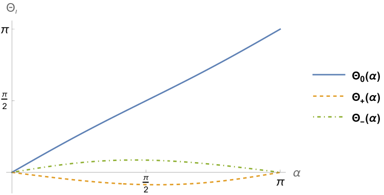
(a)

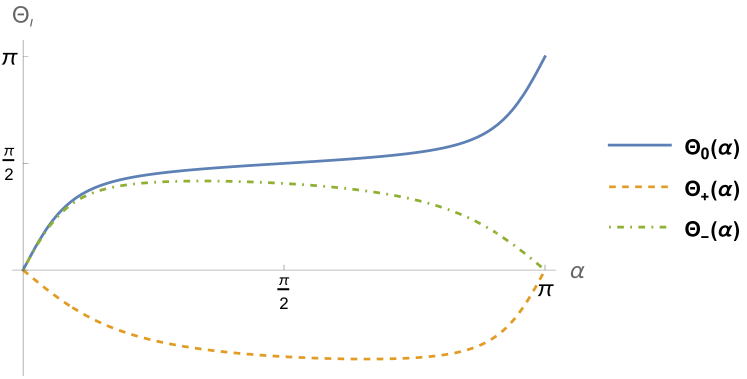
(b)

Figure 1: Scattering phases $\Theta_{\iota}(\alpha)$, with $\iota=0,\pm$, defined by (58c), (58d), versus the rapidity $\alpha$ at (a) $\eta=2$, and (b) $\eta=0.3$.

The three scattering amplitudes $w_{\iota}(p_{1},p_{2})$, with $\iota=0,\pm$, can be parametrized by the rapidity variable $\alpha$,

$$w_{\iota}(p_{1},p_{2})=\exp[-i\pi+i\theta_{\iota}(p_{1},p_{2})],$$ (58a)

$$\theta_{\iota}(p_{1},p_{2})=\Theta_{\iota}(\alpha_{1}-\alpha_{2}),$$ (58b)

$$\Theta_{0}(\alpha)=\alpha+\sum_{n=1}^{\infty}\frac{e^{-n\eta}\sin(2\alpha n)}{n\cosh(n\eta)},$$ (58c)

$$\Theta_{\pm}(\alpha)=\Theta_{0}(\alpha)+\chi_{\pm}(\alpha),$$ (58d)

$$\chi_{+}(\alpha)=-i\ln\left(-\frac{\sin[(\alpha+i\eta)/2]}{\sin[(\alpha-i\eta)/2]}\right),$$ (58e)

$$\chi_{-}(\alpha)=-i\ln\left(\frac{\cos[(\alpha+i\eta)/2]}{\cos[(\alpha-i\eta)/2]}\right),$$ (58f)

where $p_{j}=p(\alpha_{j})$, $j=1,2$, and $\Theta_{\iota}(\alpha)$ are the scattering phases. Figures 1a and 1b illustrate the rapidity dependencies of the scattering phases $\Theta_{\iota}(\alpha)$ at $\eta=2$, and $\eta=0.3$, respectively. The scattering amplitude $w_{0}(p_{1},p_{2})$ was found by Zabrodin Zabrodin (1992), and the whole two-kink scattering matrix was determined by Davies et al. Davies et al. (1993).

The two-kink states $|\mathcal{K}_{\mu\nu}(\xi_{1})\mathcal{K}_{\nu\mu}(\xi_{2})\rangle_{s_{1}s_{2}}$ parametrized by the complex spectral parameters $\xi_{1,2}=-ie^{i\alpha_{1,2}}$ are simply related with $|K_{\mu\nu}(p_{1})K_{\nu\mu}(p_{2})\rangle_{s_{1}s_{2}}$:

$$|\mathcal{K}_{\mu\nu}(\xi_{1})\mathcal{K}_{\nu\mu}(\xi_{2})\rangle_{s_{1}s_{2}}=$$ (59)

$$\frac{\sqrt{\omega(p_{1})\omega(p_{2})}}{J\sinh\eta}|K_{\mu\nu}(p_{1})K_{\nu\mu}(p_{2})\rangle_{s_{1}s_{2}}.$$

The different notation $|\xi_{2},\xi_{1}\rangle_{\epsilon_{2},\epsilon_{1};(i)}$ has been commonly used Jimbo and Miwa (1995) for the two-kink states $|\mathcal{K}_{\mu\nu}(\xi_{1})\mathcal{K}_{\nu\mu}(\xi_{2})\rangle_{s_{1}s_{2}}$, with $i=\mu$, and $\epsilon_{1,2}=\mathrm{sign}\,s_{1,2}$.

The commutation relation (57) can be rewritten for the two-kink states (59) in the matrix form:

$$|\mathcal{K}_{\mu\nu}(\xi_{1})\mathcal{K}_{\nu\mu}(\xi_{2})\rangle_{s_{1}s_{2}}=\sum_{s_{1}^{\prime},s_{2}^{\prime}=\pm 1/2}\mathcal{S}_{s_{1}s_{2}}^{s_{1}^{\prime}s_{2}^{\prime}}(\alpha_{1}-\alpha_{2})\cdot$$ (60)

$$|\mathcal{K}_{\mu\nu}(\xi_{2})\mathcal{K}_{\nu\mu}(\xi_{1})\rangle_{s_{2}^{\prime}s_{1}^{\prime}}.$$

Another equivalent representation of the same commutation relation is given in the Appendix A.1 of the monograph Jimbo and Miwa (1995) by Jimbo and Miwa:

$$|\mathcal{K}_{\mu\nu}(\xi_{2})\mathcal{K}_{\nu\mu}(\xi_{1})\rangle_{s_{2}s_{1}}=$$ (61)

$$-\sum_{s_{1}^{\prime},s_{2}^{\prime}=\pm 1/2}R_{s_{1}^{\prime}s_{2}^{\prime}}^{s_{1}s_{2}}(\xi_{1}/\xi_{2})|\mathcal{K}_{\mu\nu}(\xi_{1})\mathcal{K}_{\nu\mu}(\xi_{2})\rangle_{s_{1}^{\prime}s_{2}^{\prime}},$$

$$R(\xi)=\frac{1}{\kappa(\xi)}\begin{pmatrix}1&&&\\ &\frac{(1-\xi^{2})q}{1-q^{2}\xi^{2}}&\frac{(1-q^{2})\xi}{1-q^{2}\xi^{2}}&\\ &\frac{(1-q^{2})\xi}{1-q^{2}\xi^{2}}&\frac{(1-\xi^{2})q}{1-q^{2}\xi^{2}}&\\ &&&1\end{pmatrix},$$ (62)

where $\xi_{j}=-ie^{i\alpha_{j}}$,

$$\kappa(\xi)=\xi\frac{(q^{4}\xi^{2};q^{4})\,(q^{2}\xi^{-2};q^{4})}{(q^{4}\xi^{-2};q^{4})\,(q^{2}\xi^{2};q^{4})},$$ (63)

$$\kappa(\xi_{1}/\xi_{2})=\exp[i\,\Theta_{0}(\alpha_{1}-\alpha_{2})],$$ (64)

and

$$(z;p)=\prod_{n=0}^{\infty}(1-z\,p^{n}).$$ (65)

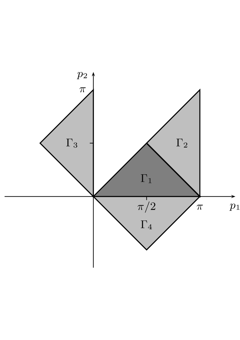
Figure 2: Integration regions $\Gamma=\Gamma_{1}\cup\Gamma_{2}$ and $\widetilde{\Gamma}=\Gamma_{1}\cup\Gamma_{4}$ in equations (51) and (68), respectively. Triangular regions $\Gamma_{2}$, $\Gamma_{3}$, and $\Gamma_{4}$ are equivalent in the sense (67).

The $\mathcal{S}$-matrix in equation (60) is simply related with the $R$-matrix in equation (61)

$$\mathcal{S}_{s_{1}s_{2}}^{s_{1}^{\prime}s_{2}^{\prime}}(\alpha_{1}-\alpha_{2})=-R_{s_{2}^{\prime}s_{1}^{\prime}}^{s_{2}s_{1}}(\xi_{2}/\xi_{1}).$$ (66)

The fundamental triangular region $\Gamma=\Gamma_{1}\cup\Gamma_{2}$ shown in Figure 2 represents an elementary cell in the two-dimensional momentum space $\mathbb{R}_{\mathbf{p}}^{2}$, $\langle p_{1},p_{2}\rangle\in\mathbb{R}_{\mathbf{p}}^{2}$. To be more specific, let us introduce the following equivalence relations in the momentum plane $\mathbb{R}_{\mathbf{p}}^{2}$:

$$\langle p_{1},p_{2}\rangle\sim\langle p_{1}+n_{1}\pi,p_{2}\rangle\sim\langle p_{1},p_{2}+n_{2}\pi\rangle\sim\langle p_{2},p_{1}\rangle,$$ (67)

with integer $n_{1},n_{2}\in\mathbb{Z}$. Denote by $\langle\langle p_{1},p_{2}\rangle\rangle$ the equivalence class of the point $\langle p_{1},p_{2}\rangle$. A region $\mathfrak{E}\subset\mathbb{R}_{\mathbf{p}}^{2}$ will be called the elementary cell in the momentum plane, if each equivalence class $\langle\langle p_{1},p_{2}\rangle\rangle\in\langle\langle\mathbb{R}_{\mathbf{p}}^{2}\rangle\rangle$ has just one representative point in $\mathfrak{E}$.

The triangular region $\Gamma$ in Figure 2 gives an example of the elementary cell. One can easily show using equations (53f) and unitarity of the two-kink scattering matrix (62), that the integration region $\Gamma$ in equations (51) can be replaced by any other elementary cell $\mathfrak{E}$. In particular, the triangular region $\Gamma$ can be replaced in (51) by the square elementary cell $\tilde{\Gamma}={\Gamma_{1}}\cup\Gamma_{4}$ shown in Figure 2. This leads to the following representation for the projection operator $\mathcal{P}_{11}^{(2)}$,

$$\mathcal{P}_{11}^{(2)}=\sum_{s_{1}=\pm 1/2\atop{s_{2}=\pm 1/2}}\iint_{\tilde{\Gamma}}\frac{dp_{1}dp_{2}}{\pi^{2}}|K_{10}(p_{1})K_{01}(p_{2})\rangle_{s_{1}s_{2}}\cdot$$ (68)

$$\phantom{.}{}_{s_{2}s_{1}}\langle K_{10}(p_{2})K_{01}(p_{1})|,$$

which will be used later.

In the Ising limit $\eta\to\infty$, the basis in the two-particle sector is formed by the localised two-kink states $|\mathbf{K}_{\mu\nu}(j_{1})\mathbf{K}_{\nu\mu}(j_{2})\rangle$, with $-\infty<j_{1}<j_{2}<\infty$. Four examples of such localized two-kink states are shown below:

$$|\mathbf{K}_{10}(2)\mathbf{K}_{01}(5)\rangle:\quad\ldots\uparrow\downarrow{\color[rgb]{0,0,1}\ \underline{\stackrel{{\scriptstyle 0}}{{\uparrow}}}}\stackrel{{\scriptstyle 1}}{{\downarrow}}{\color[rgb]{0.2,0.54,0.2}\stackrel{{\scriptstyle 2}}{{\uparrow}}}{\color[rgb]{1,0,0}\mid}{\color[rgb]{0.2,0.54,0.2}\stackrel{{\scriptstyle 3}}{{\uparrow}}}\stackrel{{\scriptstyle 4}}{{\downarrow}}{\color[rgb]{0.2,0.54,0.2}\stackrel{{\scriptstyle 5}}{{\uparrow}}}{\color[rgb]{1,0,0}\mid}{\color[rgb]{0.2,0.54,0.2}\stackrel{{\scriptstyle 6}}{{\uparrow}}}\stackrel{{\scriptstyle 7}}{{\downarrow}}\stackrel{{\scriptstyle 8}}{{\uparrow}}\ldots\quad s=1,$$

$$|\mathbf{K}_{10}(3)\mathbf{K}_{01}(6)\rangle:\quad\ldots\uparrow\downarrow{\color[rgb]{0,0,1}\ \underline{\stackrel{{\scriptstyle 0}}{{\uparrow}}}}\stackrel{{\scriptstyle 1}}{{\downarrow}}\stackrel{{\scriptstyle 2}}{{\uparrow}}{\color[rgb]{0.2,0.54,0.2}\stackrel{{\scriptstyle 3}}{{\downarrow}}}{\color[rgb]{1,0,0}\mid}{{\color[rgb]{0.2,0.54,0.2}\stackrel{{\scriptstyle 4}}{{\downarrow}}}\stackrel{{\scriptstyle 5}}{{\uparrow}}}{\color[rgb]{0.2,0.54,0.2}\stackrel{{\scriptstyle 6}}{{\downarrow}}}{\color[rgb]{1,0,0}\mid}{\color[rgb]{0.2,0.54,0.2}\stackrel{{\scriptstyle 7}}{{\downarrow}}}\stackrel{{\scriptstyle 8}}{{\uparrow}}\ldots\quad s=-1,$$

$$|\mathbf{K}_{10}(3)\mathbf{K}_{01}(7)\rangle:\quad\ldots\uparrow\downarrow{\color[rgb]{0,0,1}\ \underline{\stackrel{{\scriptstyle 0}}{{\uparrow}}}}\stackrel{{\scriptstyle 1}}{{\downarrow}}\stackrel{{\scriptstyle 2}}{{\uparrow}}{\color[rgb]{0.2,0.54,0.2}\stackrel{{\scriptstyle 3}}{{\downarrow}}}{\color[rgb]{1,0,0}\mid}{{\color[rgb]{0.2,0.54,0.2}\stackrel{{\scriptstyle 4}}{{\downarrow}}}\stackrel{{\scriptstyle 5}}{{\uparrow}}}{\color[rgb]{0,0,0}\stackrel{{\scriptstyle 6}}{{\downarrow}}}{\color[rgb]{0.2,0.54,0.2}\stackrel{{\scriptstyle 7}}{{\uparrow}}}{\color[rgb]{1,0,0}\mid}{\color[rgb]{0.2,0.54,0.2}\stackrel{{\scriptstyle 8}}{{\uparrow}}}\ldots\quad\;\;s=0,$$

$$|\mathbf{K}_{10}(2)\mathbf{K}_{01}(6)\rangle:\quad\ldots\uparrow\downarrow{\color[rgb]{0,0,1}\ \underline{\stackrel{{\scriptstyle 0}}{{\uparrow}}}}\stackrel{{\scriptstyle 1}}{{\downarrow}}{\color[rgb]{0.2,0.54,0.2}\stackrel{{\scriptstyle 2}}{{\uparrow}}}{\color[rgb]{1,0,0}\mid}{\color[rgb]{0.2,0.54,0.2}\stackrel{{\scriptstyle 3}}{{\uparrow}}}{{\color[rgb]{0,0,0}\stackrel{{\scriptstyle 4}}{{\downarrow}}}\stackrel{{\scriptstyle 5}}{{\uparrow}}}{\color[rgb]{0.2,0.54,0.2}\stackrel{{\scriptstyle 6}}{{\downarrow}}}{\color[rgb]{1,0,0}\mid}{\color[rgb]{0.2,0.54,0.2}\stackrel{{\scriptstyle 7}}{{\downarrow}}}{\color[rgb]{0,0,0}\stackrel{{\scriptstyle 8}}{{\uparrow}}}\ldots\quad\;\;s=0.$$

In the right column, $s$ stands for the ($z$-projection of the) total spin of the two-kink state. The elementary properties of these states are:

$$\langle\mathbf{K}_{\mu\nu}(j_{2})\mathbf{K}_{\nu\mu}(j_{1})|\mathbf{K}_{\mu^{\prime}\nu^{\prime}}(j_{1}^{\prime})\mathbf{K}_{\nu^{\prime}\mu^{\prime}}(j_{2}^{\prime})\rangle=\delta_{\mu\mu^{\prime}}\delta_{j_{1}j_{1}^{\prime}}\delta_{j_{2}j_{2}^{\prime}},$$

$$T_{1}|\mathbf{K}_{\mu\nu}(j_{1})\mathbf{K}_{\nu\mu}(j_{2})\rangle=|\mathbf{K}_{\nu\mu}(j_{1}-1)\mathbf{K}_{\mu\nu}(j_{2}-1)\rangle,$$

$$U|\mathbf{K}_{\mu\nu}(j_{1})\mathbf{K}_{\nu\mu}(j_{2})\rangle=|\mathbf{K}_{\nu\mu}(j_{1})\mathbf{K}_{\mu\nu}(j_{2})\rangle,$$

$$\widetilde{T}_{1}|\mathbf{K}_{\mu\nu}(j_{1})\mathbf{K}_{\nu\mu}(j_{2})\rangle=|\mathbf{K}_{\mu\nu}(j_{1}-1)\mathbf{K}_{\nu\mu}(j_{2}-1)\rangle,$$

$${H}_{I}^{(0)}|\mathbf{K}_{\mu\nu}(j_{1})\mathbf{K}_{\nu\mu}(j_{2})\rangle=4|\mathbf{K}_{\mu\nu}(j_{1})\mathbf{K}_{\nu\mu}(j_{2})\rangle.$$

The two-particle Bloch states $|K_{\mu\nu}^{I}(p_{1})K_{\nu\mu}^{I}(p_{2})\rangle_{s_{1}s_{2}}$ characterised by the quasimomenta ${p_{1},p_{2}}\in\mathbb{R}$ and the kink spins $s_{1,2}=\pm 1/2$ can be defined at $\varepsilon=0$ as follows:

$$|K_{10}^{I}(p_{1})K_{01}^{I}(p_{2})\rangle_{-1/2,-1/2}=\!\!\!\!\sum_{m_{1}=-\infty}^{\infty}\sum_{m_{2}=m_{1}}^{\infty}\!\!\Big{[}e^{2ip_{1}m_{1}+ip_{2}(2m_{2}+1)}-e^{2ip_{2}\,m_{1}+ip_{1}(2m_{2}+1)}e^{i(p_{1}-p_{2})}\Big{]}|\mathbf{K}_{10}(2m_{1}-1)\mathbf{K}_{01}(2m_{2})\rangle,$$ (69a)

$$|K_{10}^{I}(p_{1})K_{01}^{I}(p_{2})\rangle_{1/2,1/2}=\!\!\sum_{m_{1}=-\infty}^{\infty}\sum_{m_{2}=m_{1}+1}^{\infty}\!\!\Big{[}e^{ip_{1}(2m_{1}+1)+2ip_{2}m_{2}}-e^{ip_{2}(2m_{1}+1)+2ip_{1}m_{2}}e^{i(p_{1}-p_{2})}\Big{]}|\mathbf{K}_{10}(2m_{1})\mathbf{K}_{01}(2m_{2}-1)\rangle,$$ (69b)

$$|K_{10}^{I}(p_{1})K_{01}^{I}(p_{2})\rangle_{1/2,-1/2}=e^{i(p_{1}+p_{2})}\sum_{m_{1}=-\infty}^{\infty}\sum_{m_{2}=m_{1}+1}^{\infty}\Big{[}e^{ip_{1}2m_{1}+ip_{2}2m_{2}}-e^{ip_{2}2m_{1}+ip_{1}2m_{2}}\Big{]}|\mathbf{K}_{10}(2m_{1})\mathbf{K}_{01}(2m_{2})\rangle,$$ (69c)

$$|K_{10}^{I}(p_{1})K_{01}^{I}(p_{2})\rangle_{-1/2,1/2}=\!\!\!\sum_{m_{1}=-\infty}^{\infty}\sum_{m_{2}=m_{1}+1}^{\infty}\Big{[}e^{ip_{1}2m_{1}+ip_{2}2m_{2}}-e^{ip_{2}2m_{1}+ip_{1}2m_{2}}\Big{]}\,|\mathbf{K}_{10}(2m_{1}-1)\mathbf{K}_{01}(2m_{2}-1)\rangle,$$ (69d)

$$|K_{01}^{I}(p_{1})K_{10}^{I}(p_{2})\rangle_{s_{1},s_{2}}=U\,|K_{10}^{I}(p_{1})K_{01}^{I}(p_{2})\rangle_{-s_{1},-s_{2}}.$$ (69e)

Since these states have properties (51), (53), and also satisfy equations (52), and (61) to the first order in $\varepsilon$, they can be identified with the Ising limit of the two-kink eigenstates of the Hamiltonian (25):

$$\lim_{\varepsilon\to 0}|K_{\mu\nu}(p_{1})K_{\nu\mu}(p_{2})\rangle_{s_{1}s_{2}}=|K_{\mu\nu}^{I}(p_{1})K_{\nu\mu}^{I}(p_{2})\rangle_{s_{1}s_{2}}.$$ (70)

II.4 $n$-kink sector

The basis in the $n$-kink subspace $\mathcal{L}^{(n)}$ is formed by the states

$$|K_{\mu_{1}\mu_{2}}(p_{1})K_{\mu_{2}\mu_{3}}(p_{2})\ldots)K_{\mu_{n}\mu_{n+1}}(p_{n})\rangle_{s_{1}s_{2}\ldots s_{n}},$$ (71)

with $\mu_{i}=0,1$, $\mu_{i}\neq\mu_{i+1}$, $s_{i}=\pm 1/2$, and

$$0\leq p_{n}<p_{n-1}<\ldots<p_{1}<\pi.$$

Two notes are in order.

• It is not difficult to generalise equations (69) and to write the basis $n$-kink state (71) explicitly in the Ising limit $\eta\to\infty$ for any $n$ in the form of the “Bethe-Ansatz wave function”.

• Equations (20), (44), and (69) represent the zero-order terms in the Taylor $\varepsilon$-expansions of the vacuum, one-kink and two-kink eigenstates of the Hamiltonian (12). Few subsequent terms in these Taylor expansions can be straightforwardly calculated by means of the Rayleigh-Schrödinger perturbation theory in $\varepsilon\to 0$ applied to Hamiltonian (12). In particular, two initial terms in the Taylor expansion in $\varepsilon$ of the vacuum $|vac\rangle^{(1)}$ read Jimbo and Miwa (1995):

  $$|vac\rangle^{(1)}=|0\rangle^{(1)}+\frac{\varepsilon}{2}\sum_{j=-\infty}^{\infty}|K_{10}(j)K_{01}(j+2)\rangle+O(\epsilon^{2}).$$ (72)

II.5 Two-kink form factors of local spin operators

The matrix elements of local operators between the vacuum and $n$-particle basis states are commonly called “form factors”. We collect below the well-known explicit formulas for the two-kink form factors of the local spin operators $\sigma_{0}^{\pm}$ and $\sigma_{0}^{z}$.

All non-vanishing two-particle form factors of the spin operators $\sigma_{0}^{\pm},\sigma_{0}^{z}$ can be expressed in terms of four functions $X^{1}(\xi_{1},\xi_{2})$, $X^{0}(\xi_{1},\xi_{2})$, and $X_{\pm}^{z}(\xi_{1},\xi_{2})$:

$$X^{1}(\xi_{1},\xi_{2})=\phantom{.}^{(1)}\langle vac|\sigma_{0}^{+}|\mathcal{K}_{10}(\xi_{1})\mathcal{K}_{01}(\xi_{2})\rangle_{-1/2,-1/2}=$$

$$\phantom{.}{}^{(0)}\langle vac|\sigma_{0}^{-}|\mathcal{K}_{01}(\xi_{1})\mathcal{K}_{10}(\xi_{2})\rangle_{1/2,1/2},$$ (73a)

$$X^{0}(\xi_{1},\xi_{2})=\phantom{.}^{(1)}\langle vac|\sigma_{0}^{-}|\mathcal{K}_{10}(\xi_{1})\mathcal{K}_{01}(\xi_{2})\rangle_{1/2,1/2}=$$

$$\phantom{.}{}^{(0)}\langle vac|\sigma_{0}^{+}|\mathcal{K}_{01}(\xi_{1})\mathcal{K}_{10}(\xi_{2})\rangle_{-1/2,-1/2},$$ (73b)

$$X_{+}^{z}(\xi_{1},\xi_{2})=\phantom{.}^{(1)}\langle vac|\sigma_{0}^{z}|\mathcal{K}_{10}(\xi_{1})\mathcal{K}_{01}(\xi_{2})\rangle_{+}=$$

$$-\phantom{.}^{(0)}\langle vac|\sigma_{0}^{z}|\mathcal{K}_{01}(\xi_{1})\mathcal{K}_{10}(\xi_{2})\rangle_{+},$$ (73c)

$$X_{-}^{z}(\xi_{1},\xi_{2})=\phantom{.}^{(1)}\langle vac|\sigma_{0}^{z}|\mathcal{K}_{10}(\xi_{1})\mathcal{K}_{01}(\xi_{2})\rangle_{-}=$$

$$\phantom{.}{}^{(0)}\langle vac|\sigma_{0}^{z}|\mathcal{K}_{01}(\xi_{1})\mathcal{K}_{10}(\xi_{2})\rangle_{-},$$ (73d)

where $\xi_{1,2}=-i\,e^{i\alpha_{1,2}}$, and

$$|\mathcal{K}_{\mu\nu}(\xi_{1})\mathcal{K}_{\nu\mu}(\xi_{2})\rangle_{\pm}\equiv\frac{1}{\sqrt{2}}\Big{(}|\mathcal{K}_{\mu\nu}(\xi_{1})\mathcal{K}_{\nu\mu}(\xi_{2})\rangle_{1/2,-1/2}$$

$$\pm|\mathcal{K}_{\mu\nu}(\xi_{1})\mathcal{K}_{\nu\mu}(\xi_{2})\rangle_{-1/2,1/2}\Big{)}.$$ (74)

The functions $X^{j}(\xi_{1},\xi_{2})$ and $X_{\pm}^{z}(\xi_{1},\xi_{2})$ admit the following explicit representations:

$$X^{j}(\xi_{1},\xi_{2})=\rho^{2}\frac{(q^{4};q^{4})^{2}}{(q^{2};q^{2})^{3}}\cdot$$ (75)

$$\frac{(-q\xi_{1}\xi_{2})^{1-j}\xi_{\color[rgb]{0,0,0}2}\,\,\gamma(\xi_{\color[rgb]{0,0,0}2}^{2}/\xi_{\color[rgb]{0,0,0}1}^{2})\,\theta_{q^{8}}(-\xi_{1}^{-2}\xi_{2}^{-2}q^{4j})}{\theta_{q^{4}}(\xi_{1}^{-2}q^{3})\,\theta_{q^{4}}(\xi_{2}^{-2}q^{3})},$$

$$X_{+}^{z}(\xi_{1},\xi_{2})=\frac{\sqrt{2}\,e^{-\eta/4}g(\alpha_{1}+\alpha_{2},\eta)}{\sin[(\alpha_{1}-\alpha_{2}-i\eta)/2]}\,X^{0}(\xi_{1},\xi_{2}),$$ (76)

$$X_{-}^{z}(\xi_{1},\xi_{2})=-X_{+}^{z}(-\xi_{1},\xi_{2}),$$ (77)

where

$$\gamma(\xi)\equiv\frac{(q^{4}\xi;q^{4};q^{4})(\xi^{-1};q^{4};q^{4})}{(q^{6}\xi;q^{4};q^{4})(q^{2}\xi^{-1};q^{4};q^{4})},$$ (78)

$$\rho\equiv(q^{2};q^{2})^{2}\frac{(q^{4};q^{4};q^{4})}{(q^{6};q^{4};q^{4})},$$ (79)

$$(x;y;z)\equiv\prod_{m,n=0}^{\infty}(1-x\,y^{n}z^{m}),$$ (80)

$$\theta_{x}(y)=(x;x)(y;x)(xy^{-1};x),$$ (81)

$$g(\alpha,\eta)=\frac{\vartheta_{1}(\frac{\alpha}{2i\eta}|e^{-\pi^{2}/\eta})}{\vartheta_{4}(\frac{\alpha}{4i\eta}|e^{-\pi^{2}/(4\eta)})}.$$ (82)

Here $\vartheta_{i}(u|p)$ denote the elliptic theta-functions:

$$\vartheta_{1}(u|p)=2p^{1/4}\sin(\pi u)\cdot$$ (83)

$$\prod_{n=1}^{\infty}(1-p^{2n})\left(1-2p^{2n}\cos(2\pi u)+p^{4n}\right),$$

$$\vartheta_{4}(u|p)=\prod_{n=1}^{\infty}(1-p^{2n})\left(1-2p^{2n-1}\cos(2\pi u)+p^{2(2n-1)}\right),$$

$$\vartheta_{2}(u|p)=\vartheta_{1}(u+1/2|p),\quad\vartheta_{3}(u|p)=\vartheta_{4}(u+1/2|p).$$

The two-kink form factors of the $\sigma_{0}^{\pm}$ operators were determined by means of the vertex-operator formalism by Jimbo and Miwa Jimbo and Miwa (1995). In equations (75), we essentially follow the notations of Bougourzi et al. (1998); Caux et al. (2008). The explicit formulas for the form factors of the $\sigma_{0}^{z}$ operator in the XYZ spin-1/2 chain were obtained by Lashkevich Lashkevich (2002). The XXZ limit of these formulas used in (76) and (77) can be found in Dugave et al. (2015). The explicit expressions for the form factors of all three spin operators $\sigma_{0}^{\mathfrak{a}}$, $\mathfrak{a}=x,y,z$ in the XYZ spin chain were presented by Lukyanov and Terras in Lukyanov and Terras (2003).

Form factors (73) satisfy a number of symmetry relations. We shall mention some of them. The first one reads:

$$X_{\pm}^{z}(-q\xi_{1},\xi_{2})=\mp e^{i[p(\alpha_{2})-p(\alpha_{1})]}X_{\pm}^{z}(-q\xi_{2},\xi_{1}).$$ (84)

Two other equalities

$$X^{1}(\xi_{1},\xi_{2})=-X^{1}(\xi_{1},-\xi_{2})=X^{1}(-\xi_{1},\xi_{2}),$$ (85)

$$X^{0}(\xi_{1},\xi_{2})=-X^{0}(-\xi_{1},\xi_{2})=X^{0}(\xi_{1},-\xi_{2}),$$

are consistent with (53f).

The equality

$$\phantom{.}{}^{(\mu)}\langle vac|\sigma_{0}^{\mathfrak{a}}|\mathcal{K}_{\mu\nu}(-q\xi_{1})\mathcal{K}_{\nu\mu}(\xi_{2})\rangle_{s_{1},s_{2}}=$$ (86)

$$\phantom{.}{}^{(\nu)}\langle vac|\sigma_{0}^{\mathfrak{a}}|\mathcal{K}_{\nu\mu}(\xi_{2})\mathcal{K}_{\mu\nu}(-q^{-1}\xi_{1})\rangle_{s_{2},s_{1}}$$

is the particular case of the form factor “Riemann-Hilbert axiom” (356), which is discussed in Appendix B.

Note, that Jimbo and Miwa originally used in Jimbo and Miwa (1995) a different notation for the two-particle Bloch states and form factors (73), namely:

$$\phantom{.}{}^{(j)}\langle vac|\sigma_{1}^{+}|\xi_{2},\xi_{1}\rangle_{--;(j)}=X^{j}(\xi_{1},\xi_{2}),$$ (87)

In the Ising limit $\varepsilon\to 0$, the form factors (75), (76), (77) have the following leading asymptotic behavior:

$$X^{1}(\xi_{1},\xi_{2})\cong-2e^{i\alpha_{1}}\sin(\alpha_{1}-\alpha_{2}),$$

$$X^{0}(\xi_{1},\xi_{2})\cong 2\varepsilon e^{i\alpha_{1}}\sin(\alpha_{1}-\alpha_{2})\cos(\alpha_{1}+\alpha_{2}),$$

$$X_{+}^{z}(\xi_{1},\xi_{2})\cong 2\varepsilon\sqrt{2}\,e^{i(\alpha_{1}+\alpha_{2})/2}\sin(\alpha_{1}-\alpha_{2})\sin\frac{\alpha_{1}+\alpha_{2}}{2},$$

$$X_{-}^{z}(\xi_{1},\xi_{2})\cong 2i\varepsilon\sqrt{2}\,e^{i(\alpha_{1}+\alpha_{2})/2}\sin(\alpha_{1}-\alpha_{2})\cos\frac{\alpha_{1}+\alpha_{2}}{2}.$$

These asymptotical formulas can be obtained directly by means of the Rayleigh-Schrödinger perturbation theory in $\varepsilon\to 0$ applied to Hamiltonian (12), and exploiting equations (69), (70), and (72).

III Dynamical structure factors at $h=0$

Theoretical study of the dynamical spin-structure factors for the XXZ model (5) has a long history, see Caux et al. (2008) for references. In the Ising limit $\Delta\to-\infty$, both transverse and longitudinal DSFs in the two-kink approximation were calculated by Ishimura and Shiba Ishimura and Shiba (1980). For $\Delta<-1$, the calculation of the two-kink contribution to the transverse DSF by means of the vertex operator approach was initiated by Bougourzi, Karbach, and Müller Bougourzi et al. (1998), and completed by Caux, Mossel, and Castillo Caux et al. (2008). The results of calculation of the two-kink contribution to the longitudinal DSF at $\Delta<-1$ by the same method were reported recently by Castillo Castillo (2020). Later, the explicit representation for the longitudinal DSF in the antiferromagnetically ordered phase $\Delta<-1$ was obtained by Babenko et al. Babenko et al. (2021) by means of the thermal form factor expansion method.

In this Section, we describe the calculation of the two-kink contributions to the DSFs for model (5) in the gapped antiferromagnetic phase $\Delta<-1$. As in papers Bougourzi et al. (1998); Caux et al. (2008); Castillo (2020), we perform calculations in the thermodynamic limit using the vertex operator approach. However, we shall apply a slightly different, rather transparent derivation procedure, which is equally suitable for the calculation of both transverse and longitudinal DSFs at $h=0$. The same procedure will be used in Section VII for the calculation of the DFSs for model (4) in the weak confinement regime at a small $h>0$,

Let us start from the finite-size version of the XXZ spin chain model defined by the Hamiltonian

$${H}_{N}=-\frac{J}{2}\sum_{j=1}^{N}\left(\sigma_{j}^{x}\sigma_{j+1}^{x}+\sigma_{j}^{y}\sigma_{j+1}^{y}+{\Delta}\,\sigma_{j}^{z}\sigma_{j+1}^{z}\right).$$ (88)

The periodic boundary conditions are implied, and the number of sites is a multiple of four, $N\mod 4=0$. It is well known from the Bethe Ansatz solution, that model (88) has at $\Delta<-1$, aside from the true ground state $|0\rangle$, also the pseudo-vacuum state $|1\rangle$. The one-site translation operator $T_{1}$ acts on these states in the following way:

$$T_{1}|0\rangle=|0\rangle,\quad T_{1}|1\rangle=-|1\rangle,$$ (89)

and their energies become degenerate in the thermodynamic limit:

$$\lim_{N\to\infty}(E_{1}-E_{0})=0.$$

The states $|\Phi_{\mu}\rangle$, $\mu=0,1$, defined by equations

$$|\Phi_{1}\rangle=\frac{|0\rangle+|1\rangle}{\sqrt{2}},\quad|\Phi_{0}\rangle=\frac{|0\rangle-|1\rangle}{\sqrt{2}}$$

transform under the one-site translation in accordance with relations

$$T_{1}|\Phi_{1}\rangle=|\Phi_{0}\rangle,\quad T_{1}|\Phi_{0}\rangle=|\Phi_{1}\rangle,$$ (90)

which are similar to equations (21). In the thermodynamic limit, the states $|\Phi_{\mu}\rangle$ reduce to the Néel-type ordered vacua of the infinite chain:

$$\lim_{N\to\infty}|\Phi_{\mu}\rangle=|vac\rangle^{(\mu)}.$$ (91)

The dynamical structure factor in the state $|vac\rangle^{(\mu)}$ can be defined as follows Caux et al. (2008):

$${S}_{\mu}^{\mathfrak{a}\mathfrak{b}}(\mathrm{k},\omega)=\lim_{N\to\infty}\frac{1}{4N}\sum_{j_{1},j_{2}=1}^{N}e^{-i\mathrm{k}(j_{1}-j_{2})}\int_{-\infty}^{\infty}dt\,e^{i\omega t}\cdot$$

$$\langle\Phi_{\mu}|\sigma_{j_{1}}^{\mathfrak{a}}(t)\sigma_{j_{2}}^{\mathfrak{b}}(0)|\Phi_{\mu}\rangle,$$ (92)

where $\sigma_{j}^{\mathfrak{a}}(t)=e^{iH_{N}t}\sigma_{j}^{\mathfrak{a}}e^{-iH_{N}t}$.

Taking into account (9), (90), and (91), on can easily proceed in (92) to the thermodynamic limit:

$$S_{\mu}^{\mathfrak{a}\mathfrak{b}}(\mathrm{k},\omega)=\frac{1}{8}\sum_{j=-\infty}^{\infty}e^{-i\mathrm{k}j}\int_{-\infty}^{\infty}dt\,e^{i\omega t}\cdot$$ (93)

$$\Big{[}\phantom{.}^{(\mu)}\langle vac|\sigma_{j}^{\mathfrak{a}}(t)\sigma_{0}^{\mathfrak{b}}(0)|vac\rangle^{(\mu)}+$$

$$\phantom{.}{}^{(\mu)}\langle vac|\sigma_{j+1}^{\mathfrak{a}}(t)\sigma_{1}^{\mathfrak{b}}(0)|vac\rangle^{(\mu)}\Big{]},$$

where

$$\sigma_{j}^{\mathfrak{a}}(t)=e^{iHt}\sigma_{j}^{\mathfrak{a}}e^{-iHt},$$ (94)

and the Hamiltonian $H$ is given by (5).

It follows immediately from equations (23), and (9), that the right-hand side of (93) does not depend on $\mu$. So, one can drop the index $\mu$ in $S_{\mu}^{\mathfrak{a}\mathfrak{b}}(\mathrm{k},\omega)$, and define the dynamic structure factor $S^{\mathfrak{a}\mathfrak{b}}(\mathrm{k},\omega)$ in the infinite chain as follows:

$$S^{\mathfrak{a}\mathfrak{b}}(\mathrm{k},\omega)=S_{1}^{\mathfrak{a}\mathfrak{b}}(\mathrm{k},\omega).$$ (95)

The two-spinon contribution to the structure factor then takes the form

$$S_{(2)}^{\mathfrak{a}\mathfrak{b}}(\mathrm{k},\omega)=\frac{1}{8}\sum_{j=-\infty}^{\infty}e^{-i\mathrm{k}j}\int_{-\infty}^{\infty}dt\,e^{i\omega t}\cdot$$ (96)

$$\Big{[}\phantom{.}^{(1)}\langle vac|\sigma_{j}^{\mathfrak{a}}(t)\mathcal{P}_{11}^{(2)}\sigma_{0}^{\mathfrak{b}}(0)|vac\rangle^{(1)}+$$

$$\phantom{.}{}^{(1)}\langle vac|\sigma_{j+1}^{\mathfrak{a}}(t)\mathcal{P}_{11}^{(2)}\sigma_{1}^{\mathfrak{b}}(0)|vac\rangle^{(1)}\Big{]},$$

where $\mathcal{P}_{11}^{(2)}$ is the projection operator (51b) onto the two-spinon subspace $\mathcal{L}_{11}^{(2)}$.

Two dynamical structure factors are of particular importance: the transverse DSF $S^{+-}(\mathrm{k},\omega)$, and the longitudinal DSF $S^{zz}(\mathrm{k},\omega)$. Subsequent calculations of these two functions are slightly different and will be described separately.

III.0.1 Transverse DSF

After substitution of (51b) into (96) and straightforward manipulations exploiting (94) and (52) one obtains:

$$S_{(2)}^{+-}(\mathrm{k},\omega)=\frac{1}{8}\sum_{j=-\infty}^{\infty}e^{-i\mathrm{k}j}\int_{-\infty}^{\infty}dt\iint_{\tilde{\Gamma}}\frac{dp_{1}\,dp_{2}}{\pi^{2}}\,e^{i[\omega-\omega(p_{1})-\omega(p_{2})]t}\Big{[}\phantom{.}^{(1)}\langle vac|\sigma_{j}^{+}|K_{10}(p_{1})K_{01}(p_{2})\rangle_{-1/2,-1/2}\cdot$$

$$\phantom{.}{}_{-1/2,-1/2}\langle K_{10}(p_{2})K_{01}(p_{1})|\sigma_{0}^{-}|vac\rangle^{(1)}+\phantom{.}^{(1)}\langle vac|\sigma_{j+1}^{+}|K_{10}(p_{1})K_{01}(p_{2})\rangle_{-1/2,-1/2}\cdot\phantom{.}_{-1/2,-1/2}\langle K_{10}(p_{2})K_{01}(p_{1})|\sigma_{1}^{-}|vac\rangle^{(1)}\Big{]}=$$

$$\frac{\pi}{4}\,\sum_{j=-\infty}^{\infty}e^{-i\mathrm{k}j}\iint_{\tilde{\Gamma}}\frac{dp_{1}\,dp_{2}}{\pi^{2}}\delta[\omega-\omega(p_{1})-\omega(p_{2})]\Big{[}\phantom{.}^{(1)}\langle vac|\sigma_{j}^{+}|K_{10}(p_{1})K_{01}(p_{2})\rangle_{-1/2,-1/2}\cdot$$ (97)

$$\phantom{.}{}_{-1/2,-1/2}\langle K_{10}(p_{2})K_{01}(p_{1})|\sigma_{0}^{-}|vac\rangle^{(1)}+\phantom{.}^{(1)}\langle vac|\sigma_{j+1}^{+}|K_{10}(p_{1})K_{01}(p_{2})\rangle_{-1/2,-1/2}\cdot\phantom{.}_{-1/2,-1/2}\langle K_{10}(p_{2})K_{01}(p_{1})|\sigma_{1}^{-}|vac\rangle^{(1)}\Big{]}.$$

The summation over $j\in\mathbb{Z}$ in (97) can be split into two sums over even $j=2m$ and odd $j=2m+1$, with $m\in\mathbb{Z}$. Exploiting equalities

$$\widetilde{T}_{1}|vac\rangle^{(1)}=|vac\rangle^{(1)},\quad\sigma_{j+1}^{\pm}=\widetilde{T}_{1}^{-1}\sigma_{j}^{\mp}\widetilde{T}_{1},\quad\widetilde{T}_{1}|K_{10}(p_{1})K_{01}(p_{2})\rangle_{s_{1},s_{2}}=e^{i(p_{1}+p_{2})}|K_{10}(p_{1})K_{01}(p_{2})\rangle_{-s_{1},-s_{2}},$$ (98)

that follow from (23), (11), and (53d), one obtains from (97):

$$S_{(2)}^{+-}(\mathrm{k},\omega)=\frac{\pi}{4}\sum_{m=-\infty}^{\infty}\iint_{\tilde{\Gamma}}\frac{dp_{1}\,dp_{2}}{\pi^{2}}\,e^{2i\,m(p_{1}+p_{2}-\mathrm{k})}\,\delta[\omega-\omega(p_{1})-\omega(p_{2})]\Big{\{}\,\Big{[}\phantom{.}^{(1)}\langle vac|\sigma_{0}^{+}|K_{10}(p_{1})K_{01}(p_{2})\rangle_{-1/2,-1/2}\cdot$$

$$\phantom{.}{}_{-1/2,-1/2}\langle K_{10}(p_{2})K_{01}(p_{1})|\sigma_{0}^{-}|vac\rangle^{(1)}+\phantom{.}^{(1)}\langle vac|\sigma_{0}^{-}|K_{10}(p_{1})K_{01}(p_{2})\rangle_{1/2,1/2}\cdot\phantom{.}_{1/2,1/2}\langle K_{10}(p_{2})K_{01}(p_{1})|\sigma_{0}^{+}|vac\rangle^{(1)}\Big{]}+$$

$$e^{i(p_{1}+p_{2}-\mathrm{k})}\,\Big{[}\phantom{.}^{(1)}\langle vac|\sigma_{0}^{-}|K_{10}(p_{1})K_{01}(p_{2})\rangle_{1/2,1/2}\cdot\phantom{.}_{-1/2,-1/2}\langle K_{10}(p_{2})K_{01}(p_{1})|\sigma_{0}^{-}|vac\rangle^{(1)}+$$

$$\phantom{.}{}^{(1)}\langle vac|\sigma_{0}^{+}|K_{10}(p_{1})K_{01}(p_{2})\rangle_{-1/2,-1/2}\cdot\phantom{.}_{1/2,1/2}\langle K_{10}(p_{2})K_{01}(p_{1})|\sigma_{0}^{+}|vac\rangle^{(1)}\Big{]}\Big{\}}.$$ (99)

Using the Poisson summation formula

$$\sum_{m=-\infty}^{\infty}e^{2i\,mQ}=\pi\sum_{l=-\infty}^{\infty}\delta(Q-\pi l),$$ (100)

the integral representation (99) of the two-spinon transverse DSF $S_{(2)}^{+-}(\mathrm{k},\omega)$ can be simplified to the form:

$$S_{(2)}^{+-}(\mathrm{k},\omega)=\frac{1}{4}\iint_{\tilde{\Gamma}}dp_{1}dp_{2}\sum_{l=-\infty}^{\infty}\,\delta(p_{1}+p_{2}-\mathrm{k}-\pi l)\,\delta[\omega-\omega(p_{1})-\omega(p_{2})]\,\mathcal{G}^{+-}(p_{1},p_{2}|\mathrm{k})=$$

$$\frac{1}{4}\int_{0}^{\pi}dP\int_{0}^{\pi/2}dp\sum_{l=-\infty}^{\infty}\,\delta(P-\mathrm{k}-\pi l)\,\delta[\omega-\epsilon(p|P)]\,\mathcal{G}^{+-}(P/2+p,P/2-p|\mathrm{k}),$$ (101)

where

$$\mathcal{G}^{+-}(p_{1},p_{2}|\mathrm{k})=\frac{d\alpha(p_{1})}{dp_{1}}\frac{d\alpha(p_{2})}{dp_{2}}\,\Big{\{}|X^{1}(\xi_{1},\xi_{2})|^{2}+|X^{0}(\xi_{1},\xi_{2})|^{2}+$$ (102)

$$e^{i(p_{1}+p_{2}-\mathrm{k})}\Big{[}X^{0}(\xi_{1},\xi_{2})\left(X^{1}(\xi_{1},\xi_{2})\right)^{*}+\left(X^{0}(\xi_{1},\xi_{2})\right)^{*}X^{1}(\xi_{1},\xi_{2})\Big{]}\Big{\}}.$$

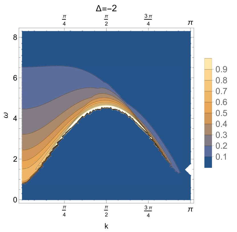
Figure 3: Two-spinon transverse DSF (106) at $\Delta=-2$, $J=1$.

Here notations (73a), (73b) have been used, $\xi_{i}=-ie^{i\alpha(p_{i})}$, $i=1,2$, and the rapidity $\alpha(p)$ corresponding to the momentum $p$ is determined by the inversion of equation (35). In equation (101), we have changed the integration variables to $P=p_{1}+p_{2}$ and $p=(p_{1}-p_{2})/2$, and used the notation

$$\epsilon(p|P)=\omega(P/2+p)+\omega(P/2-p)$$ (103)

for the total energy of two spinons. Properties of this function, which plays the key role in the subsequent analysis, are described in detail in Appendix A.

It is clear from (101), that only one term survives in the infinite sum in $l$ at any real $\mathrm{k}\notin\pi\mathbb{Z}$. This is the $l=0$ term, if $\mathrm{k}\in(0,\pi)$. In the latter case, one obtains after integration in $P$:

$$S_{(2)}^{+-}(\mathrm{k},\omega)=\int_{0}^{\pi/2}dp\,\delta[\omega-\epsilon(p|P)]\cdot$$ (104)

$$\mathcal{G}_{0}^{+-}(P/2+p,P/2-p)\Big{|}_{P=\mathrm{k}},$$

where

$$\mathcal{G}_{0}^{+-}(p_{1},p_{2})=\frac{1}{4}\frac{d\alpha(p_{1})}{dp_{1}}\frac{d\alpha(p_{2})}{dp_{2}}\,|X^{1}(\xi_{1},\xi_{2})+X^{0}(\xi_{1},\xi_{2})|^{2}.$$ (105)

The remaining integration in (III.0.2) is performed by making use of the $\delta$-function in the integrand:

$$S_{(2)}^{+-}(\mathrm{k},\omega)=\sum_{i=1}^{\mathfrak{N}(P,\omega)}\frac{\mathcal{G}_{0}^{+-}(P/2+p,P/2-p)}{|\partial_{p}\epsilon(p|P)|}\Bigg{|}_{\begin{subarray}{c}\,p=p^{(i)}\\ \!\!\!P=\mathrm{k}\end{subarray}},$$ (106)

for kinematically allowed energies

$$\omega\in\left(\min_{p}\epsilon(p|P),\max_{p}\epsilon(p|P)\right).$$ (107)

Here $p^{(i)}=p^{(i)}(P,\omega)$ are the solutions of the equation,

$$\epsilon(p|P)=\omega,$$ (108)

such that $0<p=p^{(i)}<\pi/2$, and the number $\mathfrak{N}(P,\omega)$ of such solutions takes values 1 or 2, depending on the values of $P$ and $\omega$.

It is convenient to slightly change notations for the solutions of equation (108). Namely, we shall denote the solution of (108) by $p_{a}(P,\omega)$, if $\partial_{p}\epsilon(p|P)\Big{|}_{p=p_{a}}>0$, and use the notation $p_{b}(P,\omega)$ for the solution, such that $\partial_{p}\epsilon(p|P)\Big{|}_{p=p_{b}}<0$. The solutions $p_{a,b}\in(0,\pi/2)$ of equation (108) are shown in Figure 15 in Appendix A, and their explicit expressions are given in equation (350) therein.

Figure 3 illustrates the frequency and momentum dependence of the two-spinon transverse DSF at $\Delta=-2$ calculated from equation (106). An alternative explicit representation for the same transverse DSF was obtained by Caux, Mossel, and Castillo Caux et al. (2008). There is a strong numerical evidence that both representations are equivalent: we compared numerically predictions for the transverse DSF calculated from (106) with results presented in Figure 5 of paper Caux et al. (2008) and found an excellent agreement at all $\Delta$, $\mathrm{k}$, and $\omega$.

III.0.2 Longitudinal DSF

Calculations of the longitudinal DSF are very similar to those described in Section III.0.1. The main difference is that only the two-kink configurations with zero total spin $s_{1}+s_{2}=0$ contribute to the form factor expansion of the longitudinal DSF. Proceeding to the basis (54) in the subspace of such two-kink states, we obtain from (96):

$$S_{(2)}^{zz}(\mathrm{k},\omega)=\frac{1}{8}\sum_{j=-\infty}^{\infty}e^{-i\mathrm{k}j}\int_{-\infty}^{\infty}dt\iint_{\tilde{\Gamma}}\frac{dp_{1}\,dp_{2}}{\pi^{2}}\,e^{i[\omega-\omega(p_{1})-\omega(p_{2})]t}\sum_{\iota=\pm}\Big{[}\phantom{.}^{(1)}\langle vac|\sigma_{j}^{z}|K_{10}(p_{1})K_{01}(p_{2})\rangle_{\iota}\cdot$$

$$\phantom{.}{}_{\iota}\langle K_{10}(p_{2})K_{01}(p_{1})|\sigma_{0}^{z}|vac\rangle^{(1)}+\phantom{.}^{(1)}\langle vac|\sigma_{j+1}^{z}|K_{10}(p_{1})K_{01}(p_{2})\rangle_{\iota}\cdot\phantom{.}_{\iota}\langle K_{10}(p_{2})K_{01}(p_{1})|\sigma_{1}^{z}|vac\rangle^{(1)}\Big{]}=$$

$$\frac{\pi}{4}\,\sum_{j=-\infty}^{\infty}e^{-i\mathrm{k}j}\iint_{\tilde{\Gamma}}\frac{dp_{1}\,dp_{2}}{\pi^{2}}\delta[\omega-\omega(p_{1})-\omega(p_{2})]\sum_{\iota=\pm}\Big{[}\phantom{.}^{(1)}\langle vac|\sigma_{j}^{z}|K_{10}(p_{1})K_{01}(p_{2})\rangle_{\iota}\cdot$$ (109)

$$\phantom{.}{}_{\iota}\langle K_{10}(p_{2})K_{01}(p_{1})|\sigma_{0}^{z}|vac\rangle^{(1)}+\phantom{.}^{(1)}\langle vac|\sigma_{j+1}^{z}|K_{10}(p_{1})K_{01}(p_{2})\rangle_{\iota}\cdot\phantom{.}_{\iota}\langle K_{10}(p_{2})K_{01}(p_{1})|\sigma_{1}^{z}|vac\rangle^{(1)}\Big{]}.$$

After splitting the summation over $j\in\mathbb{Z}$ into two sums over even $j=2m$ and odd $j=2m+1$, and exploiting equalities

$$\widetilde{T}_{1}|vac\rangle^{(1)}=|vac\rangle^{(1)},\quad\sigma_{j+1}^{z}=-\widetilde{T}_{1}^{-1}\sigma_{j}^{z}\widetilde{T}_{1},\quad\widetilde{T}_{1}|K_{10}(p_{1})K_{01}(p_{2})\rangle_{\iota}=\iota\,e^{i(p_{1}+p_{2})}|K_{10}(p_{1})K_{01}(p_{2})\rangle_{\iota},$$ (110)

that follow from (23), (11), and (55), one finds from (109):

$$S_{(2)}^{zz}(\mathrm{k},\omega)=\frac{\pi}{2}\sum_{m=-\infty}^{\infty}\iint_{\tilde{\Gamma}}\frac{dp_{1}\,dp_{2}}{\pi^{2}}\,e^{2i\,m(p_{1}+p_{2}-\mathrm{k})}\,\delta[\omega-\omega(p_{1})-\omega(p_{2})]\cdot$$ (111)

$$\sum_{\iota=\pm}\Big{[}\big{|}\phantom{.}^{(1)}\langle vac|\sigma_{0}^{z}|K_{10}(p_{1})K_{01}(p_{2})\rangle_{\iota}\big{|}^{2}(1-\iota\,e^{i(p_{1}+p_{2}-\mathrm{k})})\Big{]}.$$

Application of the Poisson summation formula (100) to (111) yields:

$$S_{(2)}^{zz}(\mathrm{k},\omega)=\frac{1}{2}\iint_{\tilde{\Gamma}}dp_{1}dp_{2}\sum_{l=-\infty}^{\infty}\,\delta(p_{1}+p_{2}-\mathrm{k}-\pi l)\,\delta[\omega-\omega(p_{1})-\omega(p_{2})]\,\mathcal{G}^{zz}(p_{1},p_{2}|\mathrm{k}),$$ (112)

where

$$\mathcal{G}^{zz}(p_{1},p_{2}|\mathrm{k})=\frac{d\alpha(p_{1})}{dp_{1}}\frac{d\alpha(p_{2})}{dp_{2}}\,\Big{\{}|X_{+}^{z}(\xi_{1},\xi_{2})|^{2}[1-e^{i(p_{1}+p_{2}-\mathrm{k})}]+|X_{-}^{z}(\xi_{1},\xi_{2})|^{2}[1+e^{i(p_{1}+p_{2}-\mathrm{k})}]\Big{]}\Big{\}}.$$ (113)

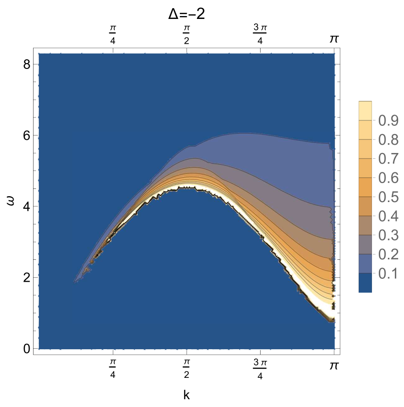
Figure 4: Two-spinon longitudinal DSF (116) at $\Delta=-2$, $J=1$.

Only the $l=0$ term survives in the infinite sum in $l$ in the right-hand side of (111) at $0\leq\mathrm{k}<\pi$. Following the steps used previously in Section III.0.1 for the calculation of the transverse DSF, one obtains

$$S_{(2)}^{zz}(\mathrm{k},\omega)=\int_{0}^{\pi/2}dp\,\delta[\omega-\epsilon(p|P)]\cdot$$ (114)

$$\mathcal{G}_{0}^{zz}(P/2+p,P/2-p)\Big{|}_{P=\mathrm{k}},$$

where

$$\mathcal{G}_{0}^{zz}(p_{1},p_{2})=\frac{d\alpha(p_{1})}{dp_{1}}\frac{d\alpha(p_{2})}{dp_{2}}\,|X_{-}^{z}(\xi_{1},\xi_{2})|^{2}.$$ (115)

Note, that the form factor $X_{+}^{z}(\xi_{1},\xi_{2})$ does not contribute to the longitudinal DSF $S_{(2)}^{zz}(\mathrm{k},\omega)$ at $0\leq\mathrm{k}<\pi$. The final result for the two-spinon longitudinal DSF for the kinematically allowed energies (107) reads

$$S_{(2)}^{zz}(\mathrm{k},\omega)=\sum_{i=1}^{\mathfrak{N}(P,\omega)}\frac{\mathcal{G}_{0}^{zz}(P/2+p,P/2-p)}{|\partial_{p}\epsilon(p|P)|}\Bigg{|}_{\begin{subarray}{c}\,p=p^{(i)}\\ \!\!\!P=\mathrm{k}\end{subarray}},$$ (116)

where the notations $p^{(i)}$ and $\mathfrak{N}(P,\omega)$, that were introduced in Section III.0.1 after equation (106), have been used.

We did not try to compare this explicit expression for the two-spinon longitudinal DSF with rather cumbersome formulas for this quantity reported by Castillo Castillo (2020), and by Babenko et al. Babenko et al. (2021). Instead, we have checked that our formula (116) perfectly reproduces the $\omega$ dependencies of the function $S_{(2)}^{zz}(\mathrm{k},\omega)$ at several fixed values of the momentum $\mathrm{k}$, which are plotted in Figure 4 in paper Babenko et al. (2021).

The frequency and momentum dependence of the two-spinon longitudinal DSF given by (116) at $\Delta=-2$ is shown in Figure 4.

IV XXZ spin chain in a weak staggered magnetic field

Application of the staggered magnetic field $h>0$ breaks integrability of the XXZ spin-chain model. It also explicitly breaks the symmetry of the model Hamiltonian (4) with respect to the inversion of all spins and to the one-site translation. However, the Hamiltonian (4) still commutes with operators $S^{z}$, $\widetilde{T}_{1}$, and $T_{2}={T}_{1}^{2}=\widetilde{T}_{1}^{2}$:

$$[\mathcal{H}(h),S^{z}]=[\mathcal{H}(h),\widetilde{T}_{1}]=[\mathcal{H}(h),{T}_{2}]=0.$$ (117)

Note also, that

$$\widetilde{T}_{1}S^{z}+S^{z}\widetilde{T}_{1}=0.$$ (118)

Let us first consider the ground state eigenvalue problem

$$\mathcal{H}_{N}(h)\,|vac(h,N)\rangle=E_{vac}(h,N)|vac(h,N)\rangle$$ (119)

for the finite-$N$ version of model model (4) defined by the Hamiltonian

$$\mathcal{H}_{N}(h) =-\frac{J}{2}\sum_{j=-N/2}^{N/2-1}\!\!\left[\sigma_{j}^{x}\sigma_{j+1}^{x}+\sigma_{j}^{y}\sigma_{j+1}^{y}+\Delta\left(\sigma_{j}^{z}\sigma_{j+1}^{z}+1\right)\right]$$

$$-h\sum_{j=-N/2}^{N/2-1}(-1)^{j}\sigma_{j}^{z},$$ (120)

with even $N$, and supplemented with periodic boundary conditions.

In the thermodynamic limit, one finds by means of the straightforward perturbative analysis at small $h>0$:

$$|vac(h)\rangle\equiv\lim_{N\to\infty}|vac(h,N)\rangle=|vac\rangle^{(1)}+O(h),$$ (121)

$$e_{vac}(h)\equiv\lim_{N\to\infty}\frac{E_{vac}(h,N)}{N}=\frac{J}{2}C(\Delta)-h\,\bar{\sigma}(\eta)+O(h^{2}),$$ (122)

where $|vac\rangle^{(1)}$ is the first ground state of the infinite chain at $h=0$ determined by equations (26) and (17), $e_{vac}(h)$ is the ground-state energy per lattice site, the constant $C(\Delta)$ was defined in (24), and $\bar{\sigma}(\eta)$ is the zero-field spontaneous staggered magnetization (19).

IV.1 Classification of meson states

As in equation (25), we redefine Hamiltonian (4) by adding a constant term in order to get rid of the vacuum energy:

$$\mathcal{H}_{1}(h)=\sum_{j=-\infty}^{\infty}\!\!\bigg{\{}-\frac{J}{2}\left[\sigma_{j}^{x}\sigma_{j+1}^{x}+\sigma_{j}^{y}\sigma_{j+1}^{y}+\Delta\,\sigma_{j}^{z}\sigma_{j+1}^{z}\right]$$

$$-(-1)^{j}h\,\sigma_{j}^{z}-e_{vac}(h)\bigg{\}},$$ (123)

$$\mathcal{H}_{1}(h)|vac(h)\rangle=0.$$ (124)

The meson states $|\pi_{s,\iota,n}(P)\rangle$ can be classified by the quasimomentum $P\in[0,\pi)$, the spin $s=0,\pm 1$ and two further quantum numbers $\iota=0,\pm$, and $n=1,2,\ldots$ The quantum numbers $\iota$ and $s$ are not independent: we assign $\iota=0$ for $s=\pm 1$, and $\iota=\pm$, if $s=0$. Operators $\mathcal{H}_{1}(h)$, $T_{1}^{2}$, and $S^{z}$ act on the meson states as follows:

$$\mathcal{H}_{1}(h)|\pi_{s,\iota,n}(P)\rangle=E_{\iota,n}(P)|\pi_{s,\iota,n}(P)\rangle,$$ (125a)

$$T_{1}^{2}|\pi_{s,\iota,n}(P)\rangle=e^{2iP}|\pi_{s,\iota,n}(P)\rangle,$$ (125b)

$$S^{z}|\pi_{s,\iota,n}(P)\rangle=s|\pi_{s,\iota,n}(P)\rangle.$$ (125c)

At $h=0$, the meson states $|\pi_{s,\iota,n}(P)\rangle$ decouple into some linear combinations of two-kink states described in Section II.3:

$$|\pi_{1,0,n}(P)\rangle\to|K_{10}(p_{1})K_{01}(p_{2})\rangle_{1/2,1/2},$$

$$|\pi_{-1,0,n}(P)\rangle\to|K_{10}(p_{1})K_{01}(p_{2})\rangle_{-1/2,-1/2},$$

$$|\pi_{0,+,n}(P)\rangle\to|K_{10}(p_{1})K_{01}(p_{2})\rangle_{+},$$

$$|\pi_{0,-,n}(P)\rangle\to|K_{10}(p_{1})K_{01}(p_{2})\rangle_{-},$$

with $e^{i(p_{1}+p_{2})}=e^{iP}$.

The action of the modified translation operator $\widetilde{T}_{1}$ on the meson states can be found by combination of (125) with (117), and (118).

In the case $s=\pm 1$, with a proper choice of the overall phases of states $|\pi_{s,\iota=0,n}(P)\rangle$, one may always set up the condition

$$\widetilde{T}_{1}|\pi_{s,\iota=0,n}(P)\rangle=e^{iP}|\pi_{-s,\iota=0,n}(P)\rangle.$$ (126)

It follows immediately from (126) and (117), that the meson states $|\pi_{1,0,n}(P)\rangle$ and $|\pi_{-1,0,n}(P)\rangle$ indeed have the same energy $E_{0,n}(P)$, as it was already anticipated in (125a).

If $s=0$, the index $\iota$ can take two values $\iota=\pm$, and one should put in analogy with (55):

$$\widetilde{T}_{1}|\pi_{0,\iota,n}(P)\rangle=\iota e^{iP}|\pi_{0,\iota,n}(P)\rangle.$$ (127)

By analytical continuation of equations (125), (126), and (127) to all $P\in\mathbb{R}$, one finds:

$$|\pi_{s,\iota=0,n}(P+\pi)\rangle=e^{i\chi_{s}}|\pi_{s,\iota=0,n}(P)\rangle,$$ (128)

with $s=\pm 1$, and

$$|\pi_{s=0,\iota,n}(P+\pi)\rangle=e^{i\phi_{\iota}}|\pi_{s=0,-\iota,n}(P)\rangle,$$ (129)

with $\iota=\pm$, and some real functions $\chi_{s}(P)$, $\phi_{\iota}(P)$.

The meson energy spectra $E_{\iota,n}(P)$ must obey the following symmetry relations:

$$E_{\iota,n}(-P)=E_{\iota,n}(P),$$ (130)

$$E_{\iota,n}(P+\pi)=E_{-\iota,n}(P),$$ (131)

with $\iota=0,\pm$, $n=1,2,\ldots$, and $P\in\mathbb{R}$. One more equality

$$E_{\iota,n}(\pi-P)=E_{-\iota,n}(P)$$ (132)

is the direct consequence of (130), (131).

In what follows, we shall concentrate on the calculation of the meson energy spectra $E_{\iota,n}(P)$ in the interval $0<P<\pi/2$. Due to equalities (130)-(132), this is sufficient to determine the dispersion laws $E_{\iota,n}(P)$ at all $P\in\mathbb{R}$ .

IV.2 Heuristic calculation of the meson energy spectra

In paper Rutkevich (2018), a heuristic procedure of the calculation of the meson energy spectra in model (4) was briefly announced. Now we proceed to the detailed description of this heuristic calculation, which is based on techniques developed previously in papers Rutkevich (2008, 2010).

Let us treat the two kinks as classical particles moving along the line, and attracting one another with a linear potential. Their Hamiltonian will be taken in the form

$$H(x_{1},x_{2},p_{1},p_{2})=\omega(p_{1})+\omega(p_{2})+f\cdot(x_{2}-x_{1}),$$ (133)

where $\omega(p)$ is the kink dispersion law (30). The kink spatial coordinates $x_{1},x_{2}\in\mathbb{R}$ are subjected to the constraint

$$-\infty<x_{1}<x_{2}<\infty,$$ (134)

that results from the local ”hard-sphere interaction” of two particles at $x_{1}=x_{2}$.

After the canonical transformation

$$X=\frac{x_{1}+x_{2}}{2},\quad x=x_{1}-x_{2},$$ (135a)

$$P=p_{1}+p_{2},\quad p=\frac{p_{1}-p_{2}}{2},$$ (135b)

the Hamiltonian (133) takes the form

$$H(p,x|P)=\epsilon(p|P)-f\,x,$$ (136)

where $\epsilon(p|P)$ is given by (103), and $x<0$.

The total energy-momentum conservation laws read:

$$\epsilon(p(t)|P)-f\,x(t)=E=Const,$$ (137)

$$P(t)=Const.$$ (138)

The classical evolution in the “center of mass frame” is determined by the canonical equations of motion:

$$\dot{X}(t)=\frac{\partial\epsilon(p|P)}{\partial P},$$ (139a)

$$\dot{P}(t)=0,$$ (139b)

$$\dot{x}(t)=\frac{\partial\epsilon(p|P)}{\partial p},$$ (139c)

$$\dot{p}(t)=f.$$ (139d)

This classical evolution strongly depends on the values of the conserved total momentum $P$, and energy $E$.

Let us start from the case of a small enough total momentum $P$ of two particles:

$$0\leq P\leq P_{c}(\eta),$$ (140)

where the critical momentum $P_{c}(\eta)$ is given by (337). In this case, the kinetic energy $\epsilon(p|P)$ monotonically increases in $p$ in the interval $(0,\pi/2)$, see Figure 5b. The dynamics of the system is qualitatively different in two regimes:

$$\epsilon(0|P)<E<\epsilon(\pi/2|P),$$ (141)

and

$$E>\epsilon(\pi/2|P).$$ (142)

1. In the first regime (140), (141), equation $\epsilon(p|P)=E$ has two solutions $p=\pm p_{a}$ bounding the kinematically allowed region

   $$-p_{a}<p<p_{a}$$ (143)

   in the interval $p\in(-\pi/2,\pi/2)$ of the momentum $p$ variable, see Figure 5b. Let us choose the initial conditions for equations (139c), (139d) as follows: $x(0)=0$ and $p(0)=-p_{a}<0$, see Figure 5. Due to (139d), the momentum $p$ linearly increases in time $p(t)=-p_{a}+f\,t$ until the moment

   $$t_{1}=\frac{2p_{a}}{f},$$ (144)

   when $p(t)$ reaches the value $p(t_{1}-0)=p_{a}>0$. The spatial coordinate $x$, in turn, decreases from the value $x(0)=0$ to its minimal value

   $$x_{min}=\frac{\epsilon(0|P)-E}{f}<0$$ (145)

   at $t=t_{1}/2$, and then increases up to the initial zero value at the time moment $t_{1}$, $x(t_{1})=0$. After the subsequent elastic reflection from the infinite potential well at $x=0$, the momentum changes its sign: $p(t_{1}+0)=-p(t_{1}-0)=-p_{a}$. Then the whole cycle described above repeats. So, in this first regime, the coordinate $x(t)$ and the momentum $p(t)$ of the relative motion of two particles are periodic functions of time with period $t_{1}$, and

   $$p(t)=-p_{a}+\{{t}/{t_{1}}\}\,t_{1}\,f,\quad\text{at }t>0,$$ (146)

   where $\{z\}$ denotes the fractional part of $z$.

   

   (a) Evolution in the spacial coordinate $x$.

   

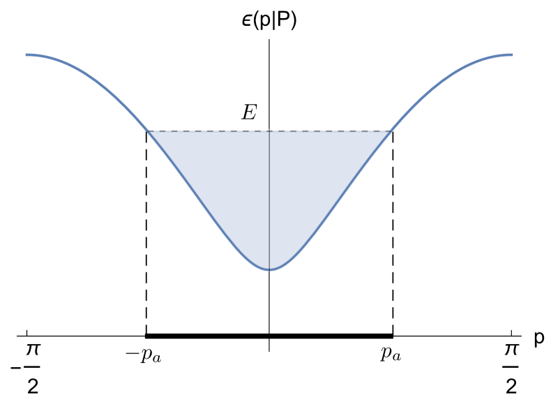
   (b) Evolution in the momentum $p$.

   Figure 5: Evolution of the classical Hamiltonian system (139c), (139d) in spatial coordinate $x$ (a), and in momentum $p$ (b), at $P=0$ in the first dynamical regime (141).

   Figure 6 illustrates the “lentils-pod-like” world paths $x_{1}(t)<x_{2}(t)$ of two particles in the first dynamical regime. One can easily see from the canonical equations of motion (139), that both particles drift together in this regime with the average velocity

   $$\langle\dot{X}\rangle:=\frac{1}{t_{1}}\int_{0}^{t_{1}}dt\,\dot{X}(t)=\frac{\omega(p_{1a})-\omega(p_{2a})}{p_{1a}-p_{2a}},$$ (147)

   where

   $$p_{1a}=P/2+p_{a},\quad p_{2a}=P/2-p_{a}.$$ (148)

   

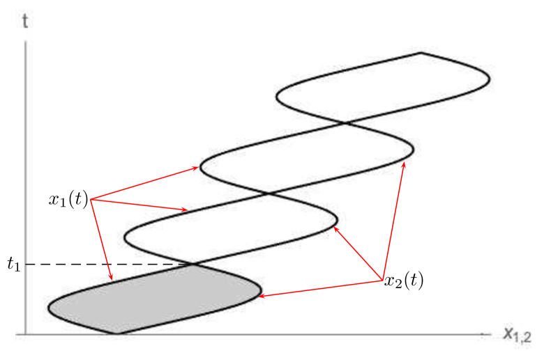
   Figure 6: Lentils-pod-like world paths $x_{1}(t)$ and $x_{2}(t)$ of two particles in the first regime. The dynamics of the particles is determined by the Hamiltonian (133), the period $t_{1}$ is given by (144).

2. At higher energies (142), the kinematically allowed regions in the $p$-variable extend to the whole real axis. The momentum $p(t)$ linearly increases with time

   $$p(t)=p(0)+f\,t,\quad t\in\mathbb{R},$$ (149)

   while the coordinate $x(t)$ oscillates in the interval $x_{min}\leq x(t)\leq x_{max}$, where $x_{min}$ is given by (145), and

   $$x_{max}=\frac{\epsilon(\pi/2|P)-E}{f}.$$ (150)

   Since $x_{max}<0$, the two kinks never meet and display periodic Bloch oscillations Bloch (1929) along the spin chain with time period $t_{2}={\pi}/{f}$. Figure 7 shows such Bloch oscillations of two particles in real space. The time-dependencies of their spatial coordinates can be easily found explicitly:

   $$x_{1}(t)=f^{-1}\,\omega(ft+p_{10})+C_{1},$$ (151)

   $$x_{2}(t)=-f^{-1}\,\omega(-ft+p_{20})+C_{2},$$

   where

   $$p_{10}+p_{20}=P,$$ (152)

   $$C_{2}-C_{1}=E/f.$$ (153)

   The kinks do not drift along the chain in the this regime:

   $$\langle\dot{X}\rangle:=\int_{t}^{t+t_{2}}dt^{\prime}\,\dot{X}(t^{\prime})=0.$$ (154)

   

   Figure 7: Bloch oscillations of two particles in the second dynamical regime. The period of oscillation is $\pi/f$, $x_{1}(t)$ and $x_{1}(t)$ are given by (151).

At

$$P_{c}(\eta)<P<\pi/2,$$ (155)

the profile of the function $\epsilon(p|P)$ changes, as it is described in Appendix A and shown in Figure 15a. In this case, the function $\epsilon(p|P)$ has a local maximum at $p=0$, and takes its minimum value $\epsilon_{m}(P,\eta)$ at $p=\pm p_{m}(P,\eta)$ where $p_{m}(P,\eta)$ and $\epsilon_{m}(P,\eta)$ are given by equations (340), and (339), respectively. As the result, the classical evolution of the system in the third regime under condition (155) and

$$\epsilon_{m}(P)<E<\epsilon(0|P)$$ (156)

becomes more complicated.

Let $p=p_{b}$, and $x=0$ at $t=0$. Then the momentum $p$ linearly increases in time

$$p(t)=p_{b}+f\,t,\quad\text{at }0<t<t_{3},$$ (157)

$$t_{3}=\frac{p_{a}-p_{b}}{f},$$ (158)

in the right lacuna in Figure 8, and at $t=t_{3}$ reaches the value $p_{a}$. During the time interval $(0,t_{3})$, the spatial coordinate decreases to the value $x_{min}=[\epsilon_{m}(P)-E]/f<0$, and then returns to the initial zero value: $x(t_{3})=0$. After the elastic reflection from the infinite potential wall at $x=0$, the sign of the momentum $p$ changes: $p(t_{3}+0)=-p_{a}$. During the subsequent time interval $t_{3}<t<2t_{3}$, the momentum $p$ linearly increases in time in the left lacuna,

$$p(t)=-p_{a}+f\,t,$$ (159)

By the end of this time interval $p(2t_{3}-0)=-p_{b}$, and $x(2t_{3})=0$. After the second scattering from the infinite potential wall at $x=0$, the momentum changes the sign and returns to its initial value: $p(2t_{3}+0)=p_{b}$. So, the momentum $p(t)$ and the spatial coordinate $x(t)$ are periodic functions of time with period $2t_{3}$.

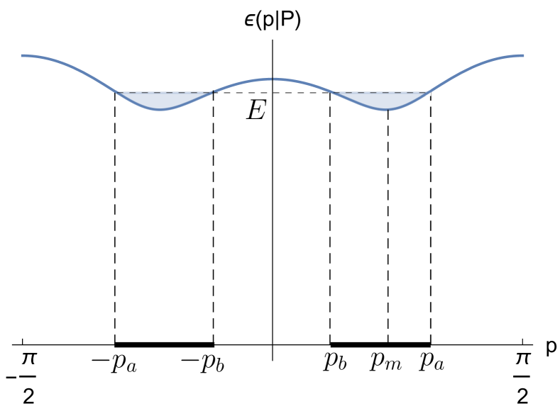
Figure 8: Two kinematically allowed regions $(-p_{a},-p_{b})$ and $(p_{b},p_{a})$ in the third dynamical regime (155), (156).

Evolution of the spatial coordinates of two particles in this third regime is shown in Figure 9. The two particles drift together with the average velocity

$$\langle\dot{X}\rangle=\frac{\omega(p_{1a})-\omega(p_{1b})-\omega(p_{2a})+\omega(p_{2b)}}{2(p_{1a}-p_{1b})},$$ (160)

where

$$p_{1b}=P/2+p_{b},\quad p_{2b}=P/2-p_{b}.$$ (161)

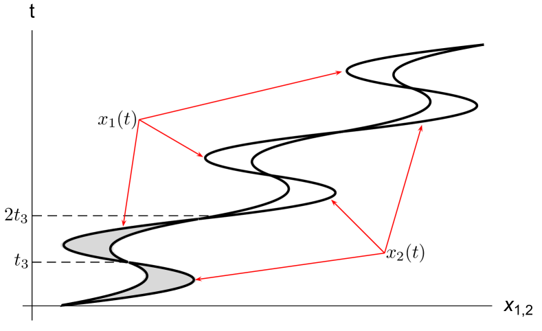
Figure 9: World paths $x_{1}(t)$ and $x_{2}(t)$ of two particles in the third dynamical regime. The half-period $t_{3}$ is given by (158).

With increasing energy, the points $-p_{b}$ and $p_{b}$ in Figure 8 approach one another, and finally merge in the origin, when the energy exceeds the value $E=\epsilon(0|P)$. At higher energies in the interval

$$\epsilon(0|P)<E<\epsilon(\pi/2|P),$$ (162)

the kinematically allowed region fills the interval $(-p_{a},p_{a})$, and the classical evolution of the system is described by equations (144), (146), and (147), corresponding to the regime (I). Upon further increase of the energy into the interval (142), the system falls into the Bloch oscillatory regime (II) characterized by equations (151) and (154).

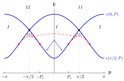
Figure 10: Structure of the meson energy spectra in the energy-momentum plane. Detailed explanations are in the text.

It is straightforward to extend the analysis described above from the interval $(0,\pi/2)$ of the total momentum to all $P\in\mathbb{R}$. The result is illustrated in Figure 10, which shows the regions in the $PE$-plane, where the dynamical regimes (I), (II), and (III) are realized. The whole diagram is symmetric with respect to the reflection $P\to-P$ and $\pi$-periodic in the momentum $P$. Two solid blue curves in Figure 10 plot the functions $\epsilon(0,P)$, and $\epsilon(\pi/2,P)$. The right dashed red curve displays the function $\epsilon_{m}(P)$ in the interval $P_{c}<P<\pi-P_{c}$, where $\epsilon_{m}(P)$ and $P_{c}$ are given by (339) and (337), respectively. The left dashes red curve is the mirror reflection of the right one with respect to the ordinate axis. The whole diagram in Figure 10 corresponds to a generic fixed value of the parameter $\eta>0$.

Let us now turn to the quantization of the Hamiltonian dynamics described above. Two approximate schemes can be used at small $f>0$.

IV.2.1 Semiclassical quantization

In order to quantize the states well inside the regions (I), (II), or (III) in Figure 10 far enough from their boundaries, it is natural to use the semiclassical Bohr-Sommerfeld quantization rule. This rule states, that the increase of the phase $\Delta\Phi$ of the semiclassical wave-function corresponding to one cycle of the periodical phase trajectory $x(t),p(t)$ in some potential well profile must be a multiple of $2\pi$:

$$\Delta\Phi=2\pi n.$$ (163)

In the first dynamical regime (I), the phase shift $\Delta\Phi$ consists of three terms,

$$\Delta\Phi=\Delta_{1}\Phi+\Delta_{2}\Phi+\Delta_{3}\Phi,$$ (164)

where the first one

$$\Delta_{1}\Phi=\oint dx\,p(x)$$ (165)

is associated with the one cycle of the classical movement over the closed periodical phase trajectory, and the second one

$$\Delta_{2}\Phi=\frac{\pi}{2}$$ (166)

represents the familiar phase shift of the wave function at the left turning point $x_{min}$, see Figure 5a and ref. [Landau and Lifshitz, 1981]. The third phase shift $\Delta_{3}\Phi$ is associated with the right turning point $x=0$. It results from the mutual elastic scattering of two kinks, that meet together at some point $x_{1}=x_{2}$. Just before their collision, the left and the right kinks had momenta $p_{1a}$ and $p_{2a}$ given by equation (148), $p_{1a}>p_{2a}$. After the collision, the left and the right kinks get momenta $p_{2a}$, and $p_{1a}$, respectively. Accordingly, the phase shift $\Delta_{3}\Phi$ must be identified (to the zero order in $f$) with the scattering phase (58) of the $\iota$-th meson mode:

$$\Delta_{3}\Phi=\theta_{\iota}(p_{1a},p_{2a}),$$ (167)

where $\iota=0,\pm$. So, the WKB energy levels $E_{\iota,n}(P)$ (with $n\gg 1$) of the $\iota$-th meson mode are determined in the first dynamical regime by the quantization condition:

$$\Delta_{1}\Phi+\frac{\pi}{2}+\theta_{\iota}\left(P/2+p_{a},P/2-p_{a}\right)=2\pi n,$$ (168)

where $n$ is the number of the energy level, $n=1,2,\ldots$.

The phase shift $\Delta_{1}\Phi$ defined by (165) can be rewritten as

$$\Delta_{1}\Phi=2\int_{x_{min}}^{0}dx\,p(x),$$ (169)

where the momentum $p(x)$ monotonically increases with $x$ from zero at the left turning point $p(x_{min})=0$, to the positive value $p(0)=p_{a}>0$ at the right turning point. The integral in the right-hand side of (169) can be further transformed as follows:

$$\Delta_{1}\Phi=2\int_{0}^{p_{a}}dp\,\,\frac{dx(p)}{dp}\,\,p=\frac{2}{f}\int_{0}^{p_{a}}dp\,\,\dot{x}\,p=$$ (170)

$$\frac{2}{f}\int_{0}^{p_{a}}dp\,\,\frac{\partial\epsilon(p|P)}{\partial p}\,p=\frac{1}{f}\left[2E_{\iota,n}(P)\,p_{a}-\int_{-p_{a}}^{p_{a}}dp\,\epsilon(p|P)\right].$$

The canonical equations of motion (139d) and (139c) have been used in the second and third equalities, respectively. In the last equality, we have integrated by parts, and then used equation

$$E_{\iota,n}(P)=\epsilon(\pm p_{a}|P).$$ (171)

Thus, the semiclassical quantization rule (168) predicts the following energy spectrum of the two-kink bound states in the first regime:

$$2E_{\iota,n}(P)\,p_{a}-\int_{-p_{a}}^{p_{a}}dp\,\epsilon(p|P)=$$ (172)

$$f\left[2\pi\,(n-1/4)-\theta_{\iota}\left(P/2+p_{a},P/2-p_{a}\right)\right].$$

The quantity $f\,\Delta_{1}\Phi$ standing in the left-hand side of this equation equals at $E=E_{\iota,n}(P)$ to the area of the dashed region in Figure 5b. On the other hand, the ratio $\Delta_{1}\Phi/f$ admits an alternative geometrical interpretation:

$$\frac{\Delta_{1}\Phi}{f}=\frac{1}{f}\oint p\,dx=-\frac{1}{f}\oint x\,dp=-\frac{1}{f}\int_{-p_{a}}^{p_{a}}x\,dp=$$

$$-\int_{0}^{t_{1}}x(t)\,dt=\int_{0}^{t_{1}}[x_{2}(t)-x_{1}(t)]\,dt=S,$$

where $S$ is the area of the dashed ”lentil seed” in Figure 6.

In the third (III) dynamical regime, the functions $p(t)$ and $x(t)$ are periodic with the period $2t_{3}$, and one can still use the Bohr-Sommerfeld rule (163), and equations (164), (165) for the semiclassical quantization. However, now the three terms in the right-hand side of (164) split into two contributions corresponding to the left and right lacunas in Figure 8:

$$\Delta_{i}\Phi=\Delta_{i}^{(l)}\Phi+\Delta_{i}^{(r)}\Phi,$$

where $i=1,2,3$, and

$$\Delta_{1}^{(l)}\Phi=\Delta_{1}^{(r)}\Phi=$$

$$\frac{1}{f}\left[E_{\iota,n}(P)\,(p_{a}-p_{b})-\int_{p_{b}}^{p_{a}}dp\,\epsilon(p|P)\right],$$

$$\Delta_{2}^{(l)}\Phi=\Delta_{2}^{(r)}\Phi=\frac{\pi}{2},$$

$$\Delta_{3}^{(l)}\Phi=\theta_{\iota}(p_{2b},p_{1b}),\quad\Delta_{3}^{(r)}\Phi=\theta_{\iota}(p_{1a},p_{2a}).$$

Thus, the the Bohr-Sommerfeld semiclassical quantization rule (163) leads in the third regime to the following energy spectrum $E_{\iota,n}(P)$ of the $\iota$-th two-kink bound-states mode:

$$2E_{\iota,n}(P)\,(p_{a}-p_{b})-2\int_{p_{b}}^{p_{a}}dp\,\epsilon(p|P)=f\bigg{[}2\pi\,(n-1/2)-$$ (173)

$${\theta_{\iota}\left(P/2+p_{a},P/2-p_{a}\right)+\theta_{\iota}\left(P/2+p_{b},P/2-p_{b}\right)}\bigg{]},$$

$$E_{\iota,n}(P)=\epsilon(p_{a}|P)=\epsilon(p_{b}|P).$$

Note, that quantities $f\,\Delta_{1}\Phi$ and $\Delta_{1}\Phi/f$ are now equal to the areas of the dashed regions in Figure 8, and Figure 9, respectively.

The Bohr-Sommerfeld quantization rule (163) cannot be directly applied in the second dynamical regime, since the momentum $p(t)$ monotonically increases with time (see (139d)), and, therefore, the phase trajectories in the $(x,p)$-plane are not closed. Nevertheless, the semiclassical energy spectra $E_{\iota,n}(P)$ can be partly recovered by means of the following simple arguments Rutkevich (2008).

In the second (II) dynamical regime, the two kinks do not meet together, and oscillate around certain positions $\bar{x}_{1}$ and $\bar{x}_{2}$ in the spin chain, see Figure 7. These two kinks cannot drift along the chain, and, therefore, the velocity $v_{\iota,n}(P)$ of their bound state is zero. Since $v_{\iota,n}(P)=\partial E_{\iota,n}(P)/\partial P=0$, the energy $E_{\iota,n}(P)$ does not depend on $P$. On the other hand, it is clear from equations (151), (153), that the shift of the second kink to the right by $\Delta x$:

$$\bar{x}_{1}\to\bar{x}_{1},\quad\bar{x}_{2}\to\bar{x}_{2}+\Delta x,$$ (174)

leads to the proportional increase of the two-kink energy:

$$E\to E+f\Delta x.$$ (175)

Recalling that the spin chain is discrete with unit lattice spacing, and the antiferromagnetic ground state is invariant with respect to the translation by two lattice sites, we can argue, that the translation parameter $\Delta x$ in equations (174) and (175) must take integer even values. As a result, the energy spectrum of the two-kink bound states in the second semiclassical regime must form the equidistant Zeeman ladders

$$E_{\iota,n}(P)=2nf+A_{\iota},$$ (176)

with some constants $A_{\iota}$. These constants will be determined later (see equation (285)) in Section VI.1. Equation (285) will be derived in Appendix D.2 in the more rigorous approach based on the Bethe-Salpeter equation.

Equations (172), (176), and (173), represent the leading terms of the semiclassical expansions in integer powers of $f\to 0$ of the meson energy spectra $E_{\iota,n}(P)$, that hold well inside the regions (I), (II), and (III) in Figure 10, respectively. However, these semiclassical expansions cannot be applied close to boundaries of these regions.

In the vicinity of the curves separating the region (I) from the neighboring regions (II) and (III) in Figure 10, one should use instead the crossover expansions, which will be described later in Section VI.3. On the other hand, close to the bottom boundaries of the regions (I) and (III), the small-$f$ asymptotics of the meson spectra are determined by the low energy expansions in fractional powers of $f$. Few initial terms in these expansions can be obtained by means of the canonical quantization of the Hamiltonian dynamics of the model (133).

IV.2.2 Canonical quantization

There are three low-energy expansions for the meson energy spectra, which hold at small $f$ in different regions of the $(E,P)$-plane shown in Figure 10.

1. The first low-energy expansion holds at $P\in(-P_{c}(\eta),P_{c}(\eta))$ and energies slightly above the minimal value $\epsilon(0|P)$. In this region, which is indicated by the solid blue arrows in Figure 10, the momentum $|p|<p_{a}$ is small, and the effective kinetic energy $\epsilon(p|P)$ can be expanded in $p$ to the second order:

   $$\epsilon(p|P)=\epsilon(0|P)+\frac{\epsilon^{\prime\prime}(0|P)}{2}\,p^{2}+\ldots.$$ (177)

2. The second low-energy expansion describes the meson energy spectra in the regions lying slightly above the red dashed curves in Figure 10, and indicated there by dashed red arrows. In this regime, the effective kinetic energy $\epsilon(p|P)$ has the profile of the kind shown in Figure 8, and the meson energy $E$ is slightly above the minimum value $\epsilon_{m}(P)=\epsilon(p_{m}|P)$ given by (339).

3. The third low-energy expansion holds close to the points $P=\pm P_{c}+\pi n$ with $n\in\mathbb{Z}$ at the meson energies $E$ slightly above its lower bound $\epsilon(0|P_{c})$. Corresponding profiles of the effective kinetic energy are shown by blue dashed lines in Figures 15a, 15c.

In this Section we shall restrict our attention to the first low-energy expansion and derive its first three terms using the canonical quantization of the classical dynamics determined by the Hamiltonian

$$H(p,x|P)=\epsilon(0|P)+\frac{\epsilon^{\prime\prime}(0|P)}{2}\,p^{2}-fx.$$ (178)

All three low-energy expansions will be derived later in Section VI in the more rigorous approach based on the Bethe-Salpeter equation.

So, in this Section the analysis will be restricted to the case $P\in(-P_{c}(\eta),P_{c}(\eta))$, with a small positive $E-\epsilon(0|P)$. After the replacement $p\to-i\partial_{x}$, the classical Hamiltonian (178) describing the relative motion of two kinks, transforms into its quantum counterpart:

$$\hat{H}=\epsilon(0|P)-\frac{\epsilon^{\prime\prime}(0|P)}{2}\partial_{x}^{2}-f\,x.$$ (179)

This second-order differential operator acts on the wave functions $\psi(x)$ that vary in the half-line $x<0$ and vanish at $x\to-\infty$. The eigenvalues of the Hamiltonian (179) determine the meson energy spectrum $E_{n}(P)$ in this approximate quantization scheme. In order to complete the eigenvalue problem for $E_{n}(P)$, one has to supplement the differential equation

$$\left[\epsilon(0|P)-\frac{\epsilon^{\prime\prime}(0|P)}{2}\partial_{x}^{2}-f\,x\right]\psi_{n}(x)=E_{n}(P)\,\psi_{n}(x),$$ (180)

defined in the negative half-axis $x<0$, with the appropriate boundary condition for the eigenfunctions $\psi_{n}(x)$ at the origin $x=0$.

For particles, which are free at $f=0$, the boundary condition at $x=0$ is determined by their statistics. In the best studied free-fermionic case, which is realized in the IFT McCoy and Wu (1978); Fonseca and Zamolodchikov (2003, 2006) and in the Ising spin chain Rutkevich (2008), the relevant one is the Dirichlet boundary condition

$$\psi_{n}(0)=0.$$ (181)

The resulting energy spectrum reads in this case:

$$E_{n}(P)=\epsilon(0|P)+f^{2/3}[\epsilon^{\prime\prime}(0|P)/2]^{1/3}z_{n},$$ (182)

where $-z_{n}$, $n=1,2,\ldots$, are the zeros of the Airy function. For the IFT, the meson mass spectrum of the this structure was predicted by McCoy and Wu McCoy and Wu (1978) in 1978.

The right-hand side of (182) represents two initial terms of the low-energy expansion in integer powers of the small parameter $f^{1/3}$ for the meson energy spectrum. In the canonical quantization scheme, it is not difficult to calculate a few subsequent terms of this expansion following the procedure developed by Fonseca and Zamolodchikov for the IFT, see Appendix B of reference [Fonseca and Zamolodchikov, 2003]. One can show this way, that the next non-vanishing term in the low energy expansion for $E_{n}(P)$ in the free-fermionic case is of order $f^{4/3}$:

$$E_{n}(P)=\epsilon(0|P)+f^{2/3}[\epsilon^{\prime\prime}(0|P)/2]^{1/3}z_{n}+O(f^{4/3}),$$ (183)

cf. equation (B.19) in Fonseca and Zamolodchikov (2003).

In the case of free bosons, one should choose the Neumann boundary condition $\psi_{n}^{\prime}(0)=0$, instead of (181). As the result, the meson energy spectrum is given by equation (183), in which $z_{n}$ are replaced by the numbers $z_{n}^{\prime}$, such that $(-z_{n}^{\prime})$ are the zeros of the derivative of the Airy function.

In the case of the XXZ spin-chain (4), the choice of the boundary condition for equation (180) is not so evident, since the kinks are not free at $h=0$. Their strong short-range interaction is completely characterized at $h=0$ by the scattering amplitudes $w_{\iota}(p_{1},p_{2})$ given by equations (58). In a certain sense, these scattering amplitudes determine also the statistics of kinks due to the Faddeev-Zamolodchikov commutation relations (57). Since

$$\lim_{p_{1}\to p_{2}}w_{\iota}(p_{1},p_{2})=-1,$$ (184)

for all $\iota=0,\pm$, the kinks behave almost like free fermions in mutual scatterings with a small momentum transfer. And since only small momenta $p=(p_{1}-p_{2})/2$ are relevant in the considered low-energy dynamical regime (see equation (177)), it is tempting to assume, that the differential equation (180) should be supplemented with the Dirichlet boundary condition. However, this is not correct. We will show below, that, instead, the correct choice of the boundary condition for equation (180) is the Robin boundary condition

$$\psi(0)-a_{\iota}(P)\psi^{\prime}(0)=0,$$ (185)

where

$$a_{\iota}(P)=-\frac{1}{2}\,\partial_{p}\theta_{\iota}(P/2+p,P/2-p)\Big{|}_{p=0}=$$ (186)

$$-\frac{J\sinh\eta}{\omega(P/2)}\,\,\,\frac{d\Theta_{\iota}(\alpha)}{d\alpha}\bigg{|}_{\alpha=0}.$$

denotes the scattering length in the $\iota$-th two-kink scattering channel. With this new boundary condition, the spectrum of the Sturm-Liouville problem (180) modifies to the form:

$$E_{\iota,n}(P)=\epsilon(0|P)+f^{2/3}[\epsilon^{\prime\prime}(0|P)/2]^{1/3}z_{n}+$$ (187)

$$f\,a_{\iota}(P)+O(f^{4/3}).$$

The justification of the Robin boundary condition (185) for the differential equation (180) is the following.

The first and most important reason, is that the resulting low-energy spectrum (187) will be confirmed later in Appendix D.4 in the more consistent calculations based on the perturbative solution of the Bethe-Salpeter equation.

Second, the low-energy expansion (187) is consistent with the semiclassical expansion (172) in the following sense. Both expansions describe the small-$f$ asymptotical behavior of the meson energy spectrum $E_{\iota,n}(P)$ in the first (I) region shown in Figure 10. The semiclassical expansion (172) can be used at $n\gg 1$, while the low-energy expansion (187) holds in the narrow strip above the bottom boundary of the region (I), i.e. at small enough $E_{\iota,n}(P)-\epsilon(0|P)>0$, and $P\in(-P_{c},P_{c})$. In the crossover region, the two asymptotical expansions (172) and (187) must be equivalent. Indeed, the semiclassical asymptotical formula (172) can be reduced to the form (187) in the crossover region, using the large-$n$ asymptotics Abramowitz and Stegun (1965) for the zeros of the Airy function

$$z_{n}=\left[\frac{3\pi}{8}(4n-1)\right]^{2/3}[1+O(n^{-2})],$$ (188)

together with formulas

$$\theta_{\iota}(P/2+p_{a},P/2-p_{a})=-2p_{a}a_{\iota}(P)+O(p_{a}^{2}),$$

$$E_{\iota,n}(P)=\epsilon(0|P)+\frac{\epsilon^{\prime\prime}(0|P)}{2}p_{a}^{2}+O(p_{a}^{4}).$$

Third, equation (185) can be interpreted as the effective boundary condition arising in a certain modification of the Sturm-Liouville problem (180), (181). In order to introduce the latter, let us first modify our original phenomenological classical model of two particles by adding to its Hamiltonian (133) some interaction potential $u(x_{1}-x_{2})$, that mimics the short-range interaction between kinks in the XXZ spin chain (4) at $h=0$. Accordingly, the potential $u(x)$ should vanish at distances much larger than the correlation length $\xi$. For simplicity, we shall assume, that $u(x)=0$ at $|x|>r$, with some $r\sim\xi$. After the canonical quantization of this modified classical model under the assumptions that the two particles are fermions, we obtain the modified Sturm-Liouville problem in the half line $x<0$, consisting of the second-order differential equation

$$\left[\epsilon(0|P)-\frac{\epsilon^{\prime\prime}(0|P)}{2}\partial_{x}^{2}-f\,x+u(x)\right]\psi_{n}(x)=E_{n}(P)\,\psi_{n}(x),$$ (189)

and the Dirichlet boundary condition (181).

At $f=0$, the energy spectrum is continuous,

$$E_{p}(P)=\epsilon(0|P)+\frac{\epsilon^{\prime\prime}(0|P)}{2}p^{2},$$

and the corresponding eigenfunction can be written at $x<-r$ as

$$\psi_{p}(x)=\sin[px-\varphi(p)].$$ (190)

The scattering phase $\varphi(p)$ corresponding to the short-range potential $u(x)$ must be identified (up to the factor $1/2$) with the scattering phase (58b):

$$\varphi(p)=\frac{1}{2}\,\theta_{\iota}(P/2+p,P/2-p).$$ (191)

At small $p$, this scattering phase becomes proportional to the scattering length (186),

$$\varphi(p)=-p\,a_{\iota}(P)+O(p^{2}),$$

and the wave function (190) reduces to the form

$$\psi_{p}(x)=\sin\left\{p[x+a_{\iota}(P)]+O(p^{2})\right\}.$$ (192)

So, the wave function (190) satisfies at small $p$ the effective Dirichlet boundary condition at $x=-a_{\iota}(P)$,

$$\psi_{p}[-a_{\iota}(P)]=O(p^{2}),$$ (193)

or equivalently, the Robin boundary condition at $x=0$:

$$\psi_{p}(0)-a_{\iota}(P)\psi_{p}^{\prime}(0)=O(p^{2}).$$ (194)

At $f>0$ the solution of equation (189) vanishing at $x\to-\infty$ is given at $x<-r$ by the Airy function:

$$\psi_{n}(x)=\mathrm{Ai}\,[-z(x)],$$ (195)

where

$$z(x)=\left[\frac{2}{\epsilon^{\prime\prime}(0|P)}\right]^{1/3}f^{-2/3}\,[fx+E_{\iota,n}(P)-\epsilon(0|P)].$$ (196)

Clearly, the function (195) must satisfy at small $f\to+0$ and finite fixed $n=1,2,\ldots$, the same effective Robin boundary condition (185), as the function (192).

As in the case $f=0$, one can replace with sufficient accuracy the effective Robin boundary condition (185) for the Airy function (195) by the effective Dirichlet boundary condition in the shifted point: $\psi_{n}[-a_{\iota}(P)]=0$. The resulting characteristic equation $z[-a_{\iota}(P)]=z_{n}$, leads to the meson energy spectrum (187).

V Bethe-Salpeter equation

In this Section we derive the Bethe-Salpeter equation for the XXZ spin chain model (123) and describe its essential properties.

V.1 Two-kink approximation

The energy spectrum of mesons at $h>0$ is determined by the eigenvalue problem (125). This problem is extremely difficult, because the interaction term $\sim h$ in the Hamiltonian (123) does not conserve the number of kinks. Accordingly, the meson state solving equations (125) must contain contributions of $2n$-kink states with all $n=1,2,\ldots$:

$$|\pi_{s,\iota,n}(P)\rangle=|\pi_{s,\iota,n}^{(2)}(P)\rangle+{{|\pi_{s,\iota,n}^{(4)}(P)\rangle+\ldots}},$$

where $|\pi_{s,\iota,n}^{(2n)}(P)\rangle$ is a linear combinations of the $2n$-kink states,

$$|K_{\mu_{1}\mu_{2}}(p_{1})K_{\mu_{2}\mu_{3}}(p_{2})\ldots)K_{\mu_{2n}\mu_{2n+1}}(p_{2n})\rangle_{s_{1}s_{2}\ldots s_{2n}},$$

with $\mu_{1}=\mu_{2n+1}=1$, $s_{1}+\dots+s_{2n}=s$, and $\exp{[2i(p_{1}+\dots+p_{2n})]}=\exp{(2iP)}$. As in the cases of the IFT Fonseca and Zamolodchikov (2006) and Ising spin-chain model Rutkevich (2008), the key simplification is provided by the two-kink approximation. It implies that one replaces the exact Hamiltonian eigenvalue problem (125) by its projection onto the two-kink subspace $\mathcal{L}_{11}^{(2)}$:

$$\mathcal{H}_{1}^{(2)}(h)|\tilde{\pi}_{s,\iota,n}(P)\rangle=\tilde{E}_{\iota,n}(P)|\tilde{\pi}_{s,\iota,n}(P)\rangle,$$ (197a)

$$T_{1}^{2}|\tilde{\pi}_{s,\iota,n}(P)\rangle=e^{2iP}|\tilde{\pi}_{s,\iota,n}(P)\rangle,$$ (197b)

$$S^{z}|\tilde{\pi}_{s,\iota,n}(P)\rangle=s|\tilde{\pi}_{s,\iota,n}(P)\rangle,$$ (197c)

where

$$\mathcal{H}_{1}^{(2)}(h)=\mathcal{P}_{11}^{(2)}\sum_{j=-\infty}^{\infty}\!\!\bigg{\{}-\frac{J}{2}\big{[}\sigma_{j}^{x}\sigma_{j+1}^{x}+\sigma_{j}^{y}\sigma_{j+1}^{y}+$$

$$\Delta\,\sigma_{j}^{z}\sigma_{j+1}^{z}\big{]}-h\,[(-1)^{j}\,\sigma_{j}^{z}-\bar{\sigma}]\bigg{\}}\mathcal{P}_{11}^{(2)}.$$ (198)

Here $\mathcal{P}_{11}^{(2)}$ is the projection operator (51b) onto the two-kink subspace $\mathcal{L}_{11}^{(2)}$, and $\bar{\sigma}$ is the zero-field spontaneous magnetization (19). Tildes distinguish solutions of equations (197) from those of the exact eigenvalue problems (125).

Action of the modified translation operator $\widetilde{T}_{1}$ on the two-kink meson states $|\tilde{\pi}_{s,\iota,n}(P)\rangle$ is determined by relations

$$\widetilde{T}_{1}|\tilde{\pi}_{s,0,n}(P)\rangle=e^{iP}|\tilde{\pi}_{-s,0,n}(P)\rangle,\;\text{for }s=\pm 1,$$ (199a)

$$\widetilde{T}_{1}|\tilde{\pi}_{0,\iota,n}(P)\rangle=\iota e^{iP}|\tilde{\pi}_{0,\iota,n}(P)\rangle,\;\text{for }\iota=\pm.$$ (199b)

For $P,P^{\prime}\in[0,\pi)$, we shall normalise the meson states by the condition:

$$\langle\tilde{\pi}_{s,\iota,n}(P)|\tilde{\pi}_{s^{\prime},\iota^{\prime},n^{\prime}}(P^{\prime})\rangle=\pi\delta_{s,s^{\prime}}\delta_{\iota,\iota^{\prime}}\delta_{n,n^{\prime}}\delta(P-P^{\prime}).$$ (200)

In the momentum representation, equation (197a) takes the form:

$$[\omega(p_{1})+\omega(p_{2})-\tilde{E}(P)]\Phi_{s_{1},s_{2}}(p_{1},p_{2}|P)=$$ (201)

$$h\sum_{m=-\infty}^{\infty}\sum_{s_{1}^{\prime},s_{2}^{\prime}=\pm 1/2}\iint_{\tilde{\Gamma}}\frac{dp_{1}^{\prime}dp_{2}^{\prime}}{\pi^{2}}\,\Phi_{s_{1}^{\prime},s_{2}^{\prime}}(p_{1}^{\prime},p_{2}^{\prime}|P)\cdot$$

$$\exp[2im(p_{1}+p_{2}-p_{1}^{\prime}-p_{2}^{\prime})]\cdot$$

$$\phantom{.}{}_{s_{2}s_{1}}\langle K_{10}(p_{2})K_{01}(p_{1})|Q|K_{10}(p_{1}^{\prime})K_{01}(p_{2}^{\prime})\rangle_{s_{1}^{\prime}s_{2}^{\prime}},$$

where

$$Q=\sigma_{0}^{z}-\sigma_{1}^{z}-2\bar{\sigma},$$ (202)

the integration region $\tilde{\Gamma}$ is shown in Figure 2, and $\Phi_{s_{1},s_{2}}(p_{1},p_{2}|P)$ denotes the wave function

$$\Phi_{s_{1},s_{2}}(p_{1},p_{2}|P)=\phantom{.}_{s_{2}s_{1}}\langle K_{10}(p_{2})K_{01}(p_{1})|\tilde{\pi}(P)\rangle,$$ (203)

corresponding to the meson state $|\tilde{\pi}(P)\rangle$. It follows immediately from (53a) and (197b) that

$$\Phi_{s_{1},s_{2}}(p_{1},p_{2}|P)\left[e^{2i(P-p_{1}-p_{2})}-1\right]=0.$$ (204)

Let $p_{1}+p_{2}\in[0,\pi)$. Then equation (201) after summation over $m$ takes the form

$$[\omega(p_{1})+\omega(p_{2})-\tilde{E}(P)]\Phi_{s_{1},s_{2}}(p_{1},p_{2}|P)=$$ (205)

$$h\sum_{s_{1}^{\prime},s_{2}^{\prime}=\pm 1/2}\iint_{\tilde{\Gamma}}\frac{dp_{1}^{\prime}dp_{2}^{\prime}}{\pi}\,\delta(p_{1}+p_{2}-p_{1}^{\prime}-p_{2}^{\prime})\cdot$$

$$\phantom{.}{}_{s_{2}s_{1}}\langle K_{10}(p_{2})K_{01}(p_{1})|Q|K_{10}(p_{1}^{\prime})K_{01}(p_{2}^{\prime})\rangle_{s_{1}^{\prime}s_{2}^{\prime}}\cdot$$

$$\Phi_{s_{1}^{\prime},s_{2}^{\prime}}(p_{1}^{\prime},p_{2}^{\prime}|P).$$

The subsequent analysis will be performed separately for the cases of the meson spin $s=1$ and $s=0$.

V.2 s=1

The wave function (203) of a meson with spin $s=1$ has only one component with $s_{1}=s_{2}=1/2$. We shall use the notation $\Phi_{\iota}(p_{1},p_{2}|P)$ with $\iota=0$ for this wave function:

$$\Phi_{\iota=0}(p_{1},p_{2}|P)=\phantom{.}_{1/2,1/2}\langle K_{10}(p_{2})K_{01}(p_{1})|\tilde{\pi}_{s=1,\iota=0}(P)\rangle.$$ (206)

Due to (57a), it satisfies the following symmetry relation:

$$\Phi_{0}(p_{1},p_{2}|P)=w_{0}(p_{2},p_{1})\Phi_{0}(p_{2},p_{1}|P).$$ (207)

For $P,(p_{1}+p_{2})\in[0,\pi)$, we define the reduced meson wave function $\phi_{0}(p|P)$ by the relation:

$$\Phi_{0}(p_{1},p_{2}|P)=\pi\,e^{-ip_{1}}\,\delta(p_{1}+p_{2}-P)\,\phi_{0}\left(\frac{p_{1}-p_{2}}{2}|P\right).$$ (208)

The reduced wave function $\phi_{0}(p|P)$ can be analytically continued to the entire real axis $p\in\mathbb{R}$, where it satisfies the following symmetry relations:

$$\phi_{0}(p+\pi|P)=\phi_{0}(p|P),$$ (209)

$$\phi_{0}(-p|P)=\,\tilde{w}_{0}\!\left(P/2+p,P/2-p\right)\,\phi_{0}(p|P),$$ (210)

where $\widetilde{w}_{0}(p_{1},p_{2})=e^{i(p_{2}-p_{1})}w_{0}(p_{1},p_{2})$.

Substitution of (208) into (205) leads to the following integral equation for the function $\phi_{0}(p|P)$:

$$[\epsilon(p|P)-\tilde{E}_{\iota=0}(P)]\phi_{0}(p|P)=$$ (211)

$$\frac{4h\bar{\sigma}}{\pi}\int_{0}^{\pi/2}dp^{\prime}G_{0}(p,p^{\prime}|P)\phi_{0}(p^{\prime}|P),$$

where $\epsilon(p|P)$ is given by (103), and

$$G_{0}(p,p^{\prime}|P)=\frac{e^{i(p_{1}-p_{1}^{\prime})}}{4\bar{\sigma}}\cdot$$ (212)

$${\phantom{.}{}_{1/2,1/2}\langle K_{10}(p_{2})K_{01}(p_{1})|Q|K_{10}(p_{1}^{\prime})K_{01}(p_{2}^{\prime})\rangle_{1/2,1/2}},$$

with

$$p_{1,2}=P/2\pm p,\quad p_{1,2}^{\prime}=P/2\pm p^{\prime}.$$ (213)

The integral kernel (212) has the following symmetry properties:

$$G_{0}(p,p^{\prime}|P)=G_{0}^{*}(p^{\prime},p|P),$$ (214)

$$G_{0}(p,p^{\prime}|P)=G_{0}(p+\pi,p^{\prime}|P)=G_{0}(p,p^{\prime}+\pi|P),$$ (215)

$$G_{0}(-p,p^{\prime}|P)=\widetilde{w}_{0}(P/2+p,P/2-p)G_{0}(p,p^{\prime}|P),$$ (216)

$$G_{0}(p,-p^{\prime}|P)=\widetilde{w}_{0}(P/2-p^{\prime},P/2+p^{\prime})G_{0}(p,p^{\prime}|P).$$ (217)

It follows from equations (210) and (217) that the integrand in the right-hand side of (211) is an even function of the integration variable $p^{\prime}$. Therefore, integration in this variable in (210) can be extended to the interval $(-\pi/2,\pi/2)$:

$$[\epsilon(p|P)-\tilde{E}_{0}(P)]\phi_{0}(p|P)=$$ (218)

$${f}\int_{-\pi/2}^{\pi/2}\frac{dp^{\prime}}{\pi}\,G_{0}(p,p^{\prime}|P)\phi_{0}(p^{\prime}|P),$$

where the $f=2h\bar{\sigma}$ is the string tension, cf. Fonseca and Zamolodchikov (2006); Rutkevich (2009).

V.3 s=0

The wave function (203) of a meson with zero spin $s=0$ has two components, $\Phi_{1/2,-1/2}(p_{1},p_{2}|P)$ and $\Phi_{-1/2,1/2}(p_{1},p_{2}|P)$, which must satisfy the system of two coupled linear integral equations (205). The sum over spins $s_{1}^{\prime},s_{2}^{\prime}$ in the right-hand sides of these equations reduces to two terms due to the restriction $s_{1}^{\prime}+s_{2}^{\prime}=0$. In order to decouple these two equations, we proceed to the basis (54) in equations (203) and (205). To this end, let us first consider the scalar product

$$\phantom{.}_{\iota}\langle K_{10}(p_{2})K_{01}(p_{1})|\tilde{\pi}_{s=0,\iota^{\prime}}(P)\rangle.$$ (219)

Here and throughout this Section V.3, the indices $\iota,\iota^{\prime}$ take two values $\iota,\iota^{\prime}=\pm$. Exploiting (127), one finds:

$$\phantom{.}{}_{\iota}\langle K_{10}(p_{2})K_{01}(p_{1})|\tilde{\pi}_{s=0,\iota^{\prime}}(P)\rangle=$$ (220)

$$\phantom{.}{}_{\iota}\langle K_{10}(p_{2})K_{01}(p_{1})|\widetilde{T}_{1}^{-1}\widetilde{T}_{1}|\tilde{\pi}_{s=0,\iota^{\prime}}(P)\rangle=$$

$$\iota\,\iota^{\prime}e^{i(P-p_{1}-p_{2})}\phantom{.}_{\iota}\langle K_{10}(p_{2})K_{01}(p_{1})|\tilde{\pi}_{s=0,\iota^{\prime}}(P)\rangle.$$

Therefore, the following equality holds

$$[1-\iota\,\iota^{\prime}e^{i(P-p_{1}-p_{2})}]\phantom{.}_{\iota}\langle K_{10}(p_{2})K_{01}(p_{1})|\tilde{\pi}_{s=0,\iota^{\prime}}(P)\rangle=0,$$

for any $p_{1},p_{2},P\in\mathbb{R}$ and $\iota,\iota^{\prime}=\pm$. It is easy to understand from this equality, that, if

$$(p_{1}+p_{2}),P\in[0,\pi),$$ (221)

then (i) the scalar product (219) vanishes at $\iota\neq\iota^{\prime}$, and (ii) the scalar product (219) also vanishes at $\iota=\iota^{\prime}$, if $P\neq p_{1}+p_{2}$. This allows us to define in the region (221) the wave functions $\Phi_{\iota}(p_{1},p_{2}|P)$, $\phi_{\iota}(p|P)$ for the $s=0$ meson states with definite parity $\iota=\pm$ as follows:

$$\phantom{.}{}_{\iota}\langle K_{10}(p_{2})K_{01}(p_{1})|\tilde{\pi}_{s=0,\iota^{\prime}}(P)\rangle=\delta_{\iota\iota^{\prime}}\,\Phi_{\iota}(p_{1},p_{2}|P),$$ (222)

$$\Phi_{\iota}(p_{1},p_{2}|P)=\pi\,\delta(p_{1}+p_{2}-P)\,\phi_{\iota}\!\left(\frac{p_{1}-p_{2}}{2}|P\right).$$ (223)

Due to (57b), (56), these wave functions satisfy the following symmetry relation:

$$\Phi_{\pm}(p_{1},p_{2}|P)=w_{\pm}(p_{2},p_{1})\Phi_{\pm}(p_{2},p_{1}|P),$$ (224)

$$\phi_{\pm}(-p|P)=w_{\pm}\!\left(P/2+p,P/2-p\right)\,\phi_{\pm}(p|P),$$ (225)

$$\phi_{\pm}(p+\pi|P)=\phi_{\pm}(p|P).$$ (226)

The integral equations (205) decouple in new notations and transform to the form:

$$[\epsilon(p|P)-\tilde{E}_{\iota}(P)]\phi_{\iota}(p|P)=$$ (227)

$$\frac{4h\bar{\sigma}}{\pi}\int_{0}^{\pi/2}dp^{\prime}G_{\iota}(p,p^{\prime}|P)\phi_{\iota}(p^{\prime}|P),$$

where

$$G_{\iota}(p,p^{\prime}|P)=\frac{{\phantom{.}{}_{\iota}\langle K_{10}(p_{2})K_{01}(p_{1})|Q|K_{10}(p_{1}^{\prime})K_{01}(p_{2}^{\prime})\rangle_{\iota}}}{4\bar{\sigma}},$$ (228)

with $p_{1,2}=P/2\pm p$, and $p_{1,2}^{\prime}=P/2\pm p^{\prime}$.

The symmetry properties of the kernels (228) read:

$$G_{\iota}(p,p^{\prime}|P)=G_{\iota}^{*}(p^{\prime},p|P),$$ (229)

$$G_{\iota}(p,p^{\prime}|P)=G_{\iota}(p+\pi,p^{\prime}|P)=G_{\iota}(p,p^{\prime}+\pi|P),$$

$$G_{\iota}(-p,p^{\prime}|P)={w}_{\iota}(P/2+p,P/2-p)G_{\iota}(p,p^{\prime}|P),$$

$$G_{\iota}(p,-p^{\prime}|P)={w}_{\iota}(P/2-p^{\prime},P/2+p^{\prime})G_{\iota}(p,p^{\prime}|P).$$

The integrand in the integral in (227) is even in variable $p^{\prime}$ due to (225) and (229). Extending the integration interval in this integral to $(-\pi/2,\pi/2)$, we represent equation (227) in the form similar to (218):

$$[\epsilon(p|P)-\tilde{E}_{\iota}(P)]\phi_{\iota}(p|P)=$$ (230)

$$f\int_{{-\pi/2}}^{\pi/2}\frac{dp^{\prime}}{\pi}\,G_{\iota}(p,p^{\prime}|P)\phi_{\iota}(p^{\prime}|P).$$

V.4 s=0,1

From now on, we will permit the index $\iota$ in the Bethe-Salpeter equation (230) to take three values $\iota=0,\pm 1$. This allows us to combine the integral equations (230) with (218) and to describe in the unified manner the meson states with different spins $s$: with $s=1$ at $\iota=0$, and with $s=0$ at $\iota=\pm$.

The Bethe-Salpeter integral equations (230) constitute three eigenvalue problems that determine in the two-kink approximation three sets of the meson dispersion laws $\{\tilde{E}_{\iota,n}(P)\}_{n=1}^{\infty}$, with $\iota=0,\pm 1$, and $0\leq P<\pi$. These equations are to some extent similar to the Bethe-Salpeter equation derived in Rutkevich (2008) for the ferromagnetic Ising spin-chain model in the confinement regime, see equation (37) there.

The normalisation condition following from (200), (206), (208), (223) for the solutions of these equations reads:

$$\int_{0}^{\pi/2}\frac{dp}{\pi}\,|\phi_{\iota,n}(p|P)|^{2}=1,$$ (231)

with $\iota=0,\pm$, and $n=1,2,\ldots$.

Let us summarize some symmetry properties of functions that stand in equations (230).

• Periodicity.

  $$\epsilon(p|P)=\epsilon(p+\pi|P),$$ (232)

  $$G_{\iota}(p,p^{\prime}|P)=G_{\iota}(p+\pi,p^{\prime}|P)=G_{\iota}(p,p^{\prime}+\pi|P).$$ (233)

  $$\phi_{\iota}(p|P)=\phi_{\iota}(p+\pi|P).$$ (234)

• Complex conjugation.

  $$[G_{\iota}(p,p^{\prime}|P)]^{*}=G_{\iota}(-p,-p^{\prime}|P).$$ (235)

• Reflection symmetries.

  $$\epsilon(-p|P)=\epsilon(p|-P)=\epsilon(p|P),$$ (236)

  $$G_{\iota}(-p,p^{\prime}|P)=W_{\iota}(p|P)G_{\iota}(p,p^{\prime}|P),$$ (237)

  $$G_{\iota}(p,-p^{\prime}|P)=W_{\iota}(-p^{\prime}|P)G_{\iota}(p,p^{\prime}|P),$$ (238)

  $$\phi_{\iota}(-p|P)=W_{\iota}(p|P)\phi_{\iota}(p|P),$$ (239)

  where

  $$W_{\iota}(p|P)=\exp[-2ip\,\delta_{\iota,0}]\,w_{\iota}(P/2+p,P/2-p).$$ (240)

Note, that

$$W_{\iota}(p+\pi|P)=W_{\iota}(p|P),\text{ for }\iota=0,\pm,$$ (241a)

$$W_{0}(p+\pi/2|\pi-P)=W_{0}(p|P),$$ (241b)

$$W_{\pm}(p+\pi/2|\pi-P)=W_{\mp}(p|P).$$ (241c)

By complex conjugating equation (230) and taking into account (235), one can see that, if $\phi_{\iota}(p|P)$ solves the uniform integral equation (230), the function $[\phi_{\iota}(-p|P)]^{*}$ must solve the same equation as well. Since the solution of equation (230) is unique up to a numerical factor, we conclude that $[\phi_{\iota}(-p|P)]^{*}=C\,\phi_{\iota}(p|P)$, with some constant $C$, such that $|C|=1$. Without loss of generality, we shall put $C=-1$, yielding

$$[\phi_{\iota}(-p|P)]^{*}=-\,\phi_{\iota}(p|P).$$ (242)

It is well known Jimbo and Miwa (1995), that the two-kink matrix elements of the $\sigma_{0}^{z}$ operator

$${\phantom{.}{}_{s_{2},s_{1}}\langle K_{10}(p_{2})K_{01}(p_{1})|\sigma_{0}^{z}|K_{10}(p_{1}^{\prime})K_{01}(p_{2}^{\prime})\rangle_{s_{1}^{\prime},s_{2}^{\prime}}}$$ (243)

have the so-called kinematic singularities - simple poles at coinciding in- and out-momenta. The kinematic simple poles of the matrix element (243) with $s_{1}=s_{2}=s_{1}^{\prime}=s_{2}^{\prime}$ are located at four hyperplanes determined by any of the equalities

$$p_{1}^{\prime}=p_{1},\quad p_{2}^{\prime}=p_{2},\quad p_{1}^{\prime}=p_{2},\quad p_{2}^{\prime}=p_{1},$$ (244)

while the kinematic simple poles of (243) at $s_{1}\neq s_{2}$, $s_{1}=s_{1}^{\prime}$, $s_{2}=s_{2}^{\prime}$ lie at two hyperplanes $p_{1}^{\prime}=p_{1},$ and $p_{2}^{\prime}=p_{2}$. Accordingly, the matrix element of the operator $Q=\sigma_{0}^{z}-\sigma_{1}^{z}-2\bar{\sigma}$ in the right-hand side of (228) also has simple poles located at the hyperplanes (244). Two such simple poles merge, if $p_{1}+p_{2}=p_{1}^{\prime}+p_{2}^{\prime}$. This leads to the second order poles at $p^{\prime}=\pm p$ in the integral kernels $G_{\iota}(p,p^{\prime}|P)$ determined by (212), (228). These kernels can be represented as sums of two terms

$$G_{\iota}(p,p^{\prime}|P)=G_{\iota}^{(sing)}(p,p^{\prime}|P)+G_{\iota}^{(reg)}(p,p^{\prime}|P),$$ (245)

where (i) the first term has second order poles at $p^{\prime}=\pm p$, while the second term is regular at real $p,p^{\prime},P$; and (ii) both functions $G_{\iota}^{(sing)}(p,p^{\prime}|P)$ and $G_{\iota}^{(reg)}(p,p^{\prime}|P)$ satisfy the symmetry relations (233), (237), (238).

The explicit form of the singular part $G_{\iota}^{(sing)}(p,p^{\prime}|P)$ of the kernel is obtained in Appendix C. In order to present the final result in a compact form, we proceed to the complex variables

$$z=e^{2ip},\quad z^{\prime}=e^{2ip^{\prime}},\quad v=e^{iP},$$ (246)

and introduce the notations

$$\mathcal{G}_{\iota}(z,z^{\prime}|v)=G_{\iota}(p,p^{\prime}|P),$$ (247)

$$\mathcal{W}_{\iota}(z|v)=W_{\iota}(p|P),$$ (248)

for $\iota=0,\pm$. For any $v$ such that $|v|=1$, the functions $\mathcal{W}_{\iota}(z|v)$ are analytical and single-valued in $z$ in some open vicinity of the unit circle $S_{1}=\{z\big{|}\,|z|=1$}, and the kernels $\mathcal{G}_{\iota}(z,z^{\prime}|v)$ are single valued in the vicinity of $S_{1}\times S_{1}$.

Equation (245) in new notations takes the form

$$\mathcal{G}_{\iota}(z,z^{\prime}|v)=\mathcal{G}_{\iota}^{(sing)}(z,z^{\prime}|v)+\mathcal{G}_{\iota}^{(reg)}(z,z^{\prime}|v),$$ (249)

where $\mathcal{G}_{\iota}^{(reg)}(z,z^{\prime}|v)$ is regular in $z,z^{\prime}$ in some open vicinity of $S_{1}\times S_{1}$. For the singular term $\mathcal{G}_{\iota}^{(sing)}(z,z^{\prime}|v)$, we obtained in Appendix C the following explicit representation:

$$\mathcal{G}_{\iota}^{(sing)}(z,z^{\prime}|v)=\mathcal{G}_{\iota}^{(s)}(z,z^{\prime}|v)+\mathcal{W}_{\iota}(z^{\prime}|v)\mathcal{G}_{\iota}^{(s)}(z,z^{\prime-1}|v),$$ (250a)

$$\mathcal{G}_{\iota}^{(s)}(z,z^{\prime}|v)=-\frac{zz^{\prime}}{(z^{\prime}-ze^{-\delta})^{2}}+\frac{z\,\delta_{\iota,0}}{2(z^{\prime}-ze^{-\delta})}+$$ (250b)

$$\frac{\mathcal{W}_{\iota}(z^{\prime}|v)}{\mathcal{W}_{\iota}(z|v)}\left[-\frac{zz^{\prime}}{(z^{\prime}-ze^{\delta})^{2}}-\frac{z^{\prime}\,\delta_{\iota,0}}{2(z^{\prime}-ze^{\delta})}\right].$$

where $\delta\to+0$.

V.5 Singular integral equations in the unit circle

It is convenient to rewrite the Bethe-Salpeter equations (230) in complex variables (246):

$$[\mathcal{E}(z|v)-\Lambda_{\iota}(v)]\psi_{\iota}(z|v)=$$ (251)

$${f}\oint_{S_{1}}\frac{dz^{\prime}}{2\pi iz^{\prime}}\,\mathcal{G}_{\iota}(z,z^{\prime}|v)\psi_{\iota}(z^{\prime}|v),$$

where the unit circle $S_{1}$ in the complex variable $z^{\prime}$ is passed in the counter-clockwise direction, and

$$\mathcal{E}(z|v)=\epsilon(p|P),\quad\Lambda_{\iota}(v)=\tilde{E}_{\iota}(P),\quad\psi_{\iota}(z|v)=\phi_{\iota}(p|P).$$ (252)

The function $\mathcal{E}(z|v)$ is algebraic in $z$. Its explicit expression is given in equation (344) in Appendix A, where its analytic properties are also described in details. Here we notice only the symmetry property $\mathcal{E}(z|v)=\mathcal{E}(z^{-1}|v)$.

The wave functions $\psi_{\iota}(z|v)$ with $\iota=0,\pm$ are single-valued and analytical in some open vicinity of the unit circle $S_{1}$, and satisfy there the symmetry relations

$$\psi_{\iota}(z^{-1}|v)=\mathcal{W}_{\iota}(z|v)\psi_{\iota}(z|v),$$ (253)

$$\psi_{\iota}(z^{-1}|v)=-\psi_{\iota}^{*}(z|v).$$ (254)

Taking (249), (250a), and (253) into account, one can replace the kernel in the integrand in (251), as

$$\mathcal{G}_{\iota}(z,z^{\prime}|v)\to\widetilde{\mathcal{G}}_{\iota}(z,z^{\prime}|v)=2\mathcal{G}_{\iota}^{(s)}(z,z^{\prime}|v)+\mathcal{G}_{\iota}^{(reg)}(z,z^{\prime}|v).$$ (255)

Then, the Bethe-Salpeter equation (251) takes the final form

$$[\mathcal{E}(z|v)-\Lambda_{\iota}(v)]\psi_{\iota}(z|v)=$$ (256)

$$2{f}\oint_{S_{1}}\frac{dz^{\prime}}{2\pi iz^{\prime}}\,\mathcal{G}_{\iota}^{(s)}(z,z^{\prime}|v)\psi_{\iota}(z^{\prime}|v)+$$

$${f}\oint_{S_{1}}\frac{dz^{\prime}}{2\pi iz^{\prime}}\,\mathcal{G}_{\iota}^{(reg)}(z,z^{\prime}|v)\psi_{\iota}(z^{\prime}|v),$$

with additional constraint (253). In terms of the original momentum variables $p,p^{\prime},P$, this equation reads

$$[\epsilon(p|P)-\tilde{E}_{\iota}(P)]\phi_{\iota}(p|P)=$$ (257)

$$f\int_{{-\pi/2}}^{\pi/2}\frac{dp^{\prime}}{\pi}\,[2G_{\iota}^{(s)}(p,p^{\prime}|P)+G_{\iota}^{(reg)}(p,p^{\prime}|P)]\phi_{\iota}(p^{\prime}|P),$$

where $G_{\iota}^{(s)}(p,p^{\prime}|P)=\mathcal{G}_{\iota}^{(s)}(z,z^{\prime}|v)$.

Equation (256) belongs to the class of uniform linear singular integral equations. For the general theory of singular integral equations see the monograph Muskhelishvili (1977) by Muskhelishvili. The properties of the Bethe-Salpeter equation (256) are to much extent similar to the properties of its analogs in the IFT Fonseca and Zamolodchikov (2006) and in the Ising spin chain Rutkevich (2008). The main difference from the latter model, which is free-fermionic in the de-confined phase, is the transformation of the solution of the Bethe-Salpeter equation under the reflection $z\to z^{-1}$. The solution of equation (251) transforms according to formula (253) under this reflection, whereas the solution of the analogous Bethe-Salpeter equation corresponding to the Ising spin chain only changes its sign Rutkevich (2008).

The wave function $\psi_{\iota}(z|v)$ can be viewed as a vector in the Hilbert space with the scalar product

$$(\varphi,\psi)=\frac{1}{2\pi i}\oint_{S_{1}}\frac{dz}{z}\,\varphi^{*}(z)\,\psi(z).$$ (258)

For each $\iota=0,\pm$, and $v\in S_{1}$, the integral equation (256) constitutes the eigenvalue problem

$$\mathbf{H}_{\iota}(v)\psi_{\iota}=\Lambda_{\iota}(v)\,\psi_{\iota}$$

for the Hermitian operator $\mathbf{H}_{\iota}(v)$, defined by

$$\mathbf{H}_{\iota}(v)\psi(z)=\mathcal{E}(z|v)\psi(z)-{f}\oint_{S_{1}}\frac{dz^{\prime}}{2\pi iz^{\prime}}\,\mathcal{G}_{\iota}(z,z^{\prime}|v)\psi(z^{\prime}).$$

The operator $\mathbf{H}_{\iota}(v)$ acts in the subspace of functions satisfying the symmetry relation (253). The spectrum of the operator $\mathbf{H}_{\iota}(v)$ is real, positive, and discrete. For its eigenvalues, we shall use notations $\{\Lambda_{\iota,n}(v)\}_{n=1}^{\infty}$: $0<\Lambda_{\iota 1}(v)<\Lambda_{\iota 2}(v)\ldots$. Corresponding eigenvectors will be denoted as $\psi_{\iota,n}(z|v)$. For given $\iota$ and $v$, the eigenvectors with different $n$ are mutually orthogonal. They will be normalised by the condition

$$\frac{1}{2\pi i}\oint_{S_{1}}\frac{dz}{z}\,\psi_{\iota,n}^{*}(z|v)\,\psi_{\iota,n}(z|v)=2,$$ (259)

which is just equation (231) rewritten in the variable
$z=e^{2ip}$.

Although the eigenvalue problem (256), (253) cannot be solved exactly, it admits perturbative solutions in the weak coupling limit $f\to+0$ in different asymptotical regimes, which will be described in Section VI. In the rest of this Section, we shall introduce three auxiliary function $g_{\iota+}(z)$, $g_{\iota-}(z)$, and $U_{\iota}(z)$, which will be used later in the small-$f$ perturbative calculations of the eigenvalues $\{\Lambda_{\iota,n}(v)\}_{n=1}^{\infty}$.

First, we denote by $g_{\iota\pm}(z)$ two functions:

$$g_{\iota\pm}(z)=\oint_{S_{1}}\frac{dz^{\prime}}{2\pi i}\,\frac{\psi_{\iota}(z^{\prime})}{(z^{\prime}-z)},$$ (260)

where $g_{\iota+}(z)$ is defined at $|z|<1$, and $g_{\iota-}(z)$ is defined in the region $|z|>1$. The evident properties of these function are:

1. $g_{\iota+}(z)$ and $g_{\iota-}(z)$ are analytical at $|z|<1$ and at $|z|>1$, respectively.

2. $g_{\iota+}(z)$ and $g_{\iota-}(z)$ can be continued to the unit circle $S_{1}$, where they are continuous together with their derivatives.

3. Relation with the function $\psi_{\iota}(z)$ at $|z|=1$:

   $$\psi_{\iota}(z)=\lim_{\delta\to+0}[g_{\iota+}(ze^{-\delta})-g_{\iota-}(ze^{\delta})].$$ (261)

4. It follows from (254) and (261), that:

   $$g_{\iota\pm}^{*}(z)=-g_{\iota\mp}(z^{*}), \text{for }|z|<1,$$ (262)

   $$g_{\iota\pm}^{*}(z)=-g_{\iota\mp}(z^{-1}), \text{for }|z|=1.$$ (263)

5. The following equality holds at $|z|>1$:

   $$g_{\iota+}(z^{-1})=-\mathcal{W}_{\iota}(z)\,g_{\iota-}(z)+g_{\iota+}(0)-$$ (264)

   $$\oint_{S_{1}}\frac{dz^{\prime}}{2\pi i}\,\frac{\mathcal{W}_{\iota}(z^{\prime})-\mathcal{W}_{\iota}(z)}{(z^{\prime}-z)}\psi_{\iota}(z^{\prime}).$$

We denote by $g_{\iota,n\pm}(z|v)$ the auxiliary functions, associated according to definition (260) with the eigenfunctions $\psi_{\iota,n}(z|v)$. Exploiting equalities (254), (261), and (263), the normalisation condition (259) can be rewritten in terms of $g_{\iota,n+}(z)$:

$$\int_{-\pi/2}^{\pi/2}\frac{dp}{\pi}\,g_{\iota,n+}(z)\,g_{\iota,n+}(z^{-1})\Big{|}_{z=\exp(2ip)}=-1.$$ (265)

Let us also define one more auxiliary function $U_{\iota}(z)$ inside the unit circle $|z|<1$:

$$U_{\iota}(z)=[\mathcal{E}(z)-\Lambda_{\iota}-\delta_{\iota,0}\,f]\,g_{\iota+}(z)+2f\,z\,g_{\iota+}^{\prime}(z).$$ (266)

Its analytic properties are similar to those of the function $\mathcal{E}(z)$, since $g_{\iota+}(z)$ is analytical at $|z|<1$. The function $U_{\iota}(z)$ can be analytically continued into the region $|z|>1$, where it admits the following representation in terms of the function $g_{\iota-}(z)$:

$$U_{\iota}(z)=[\mathcal{E}(z)-\Lambda_{\iota}-\delta_{\iota,0}\,f]\,g_{\iota-}(z)-2f\,z\,g_{\iota-}^{\prime}(z)-$$

$$2f\,z\,\frac{\mathcal{W}_{\iota}^{\prime}(z)}{\mathcal{W}_{\iota}(z)}\,g_{\iota-}(z)+fX_{\iota}(z),$$ (267)

where

$$X_{\iota}(z)=\oint_{S_{1}}\frac{dz^{\prime}}{2\pi iz^{\prime}}\,\mathcal{G}_{\iota}^{(reg)}(z,z^{\prime})\psi_{\iota}(z^{\prime})-$$ (268)

$$\oint_{S_{1}}\frac{dz^{\prime}}{2\pi i}\,\frac{[\mathcal{W}_{\iota}(z^{\prime})-\mathcal{W}_{\iota}(z)-(z^{\prime}-z)\mathcal{W}_{\iota}^{\prime}(z)]}{\mathcal{W}_{\iota}(z)}\cdot$$

$$\left[\frac{2z}{(z^{\prime}-z)^{2}}+\frac{\delta_{\iota,0}}{z^{\prime}-z}\right]\psi_{\iota}(z^{\prime})\,+$$

$$\delta_{\iota,0}\left\{-g_{\iota+}(0)+\frac{\mathcal{W}_{\iota}^{\prime}(z)}{\mathcal{W}_{\iota}(z)}\lim_{z\to\infty}[z\,g_{\iota-}(z)]\right\}.$$

Note, that the integrands in the integrals in the right-hand side of (268) are regular at $z^{\prime}\in S_{1}$. To prove (267), it is sufficient to subtract (267) from (266), and to check using (261), that the resulting equation is equivalent to (256).

Equation (266) can be viewed as the first-order differential equation for the function $g_{\iota+}(z)$. The appropriate partial solution of this equation reads

$$g_{\iota+}(z)=\frac{1}{2f}\int_{0}^{z}\frac{dz^{\prime}}{z^{\prime}}\left(\frac{z}{z^{\prime}}\right)^{\delta_{\iota,0}/2}U_{\iota}(z^{\prime})\cdot$$ (269)

$$\exp\Bigg{\{}\frac{i}{2f}\,[{\mathcal{F}}(z^{\prime},\Lambda_{\iota})-{\mathcal{F}}(z,\Lambda_{\iota})]\Bigg{\}},$$

where

$${\mathcal{F}}(z,\Lambda)=\int_{z_{1}}^{z}\frac{dt}{it}\,[\mathcal{E}(t)-\Lambda].$$ (270)

As in reference Rutkevich (2008), we have to put to the origin the initial integration point in the integral in (269) in order to provide analyticity of the function $g_{\iota+}(z)$ at $z=0$. Any other choice of the initial integration point would lead to an essential singularity of the right-hand side of (269) at $z=0$. It follows from (344), (347), that the function $\mathcal{F}(z,\Lambda)$, determined by (270) is singular at $z\to 0$: ${\mathcal{F}}(z,\Lambda)\sim z^{-1/2}$. Nevertheless, the integral in $z^{\prime}$ in equation (269) converges, if the integration path lies in the physical sheet $\mathfrak{L}_{++}$ described in Appendix A, and approaches the origin along the real axis either from the right, or from the left side.

The choice of the initial point $z_{1}$ in the integral in (270) is the subject of convenience, since it has no effect on the difference $[{\mathcal{F}}(z^{\prime},\Lambda_{\iota})-{\mathcal{F}}(z,\Lambda_{\iota})]$ in the right-hand side of (269). We shall put $z_{1}=1$ for $0\leq P\leq\pi/2$, and $z_{1}=-1$ for $\pi/2<P<\pi$.

Figure 11: Closed integration contours $C_{1}$ and $C_{2}$ in equation (272) in the complex $z$-plane. Solid straight lines display the branching cuts of the function $\mathcal{E}(z)$ defined by (344).

The requirement of analyticity of the auxiliary function $g_{\iota+}(z)$ in the circle $|z|<1$ leads to two constraints:

$$J_{\beta}(\Lambda_{\iota})=0,$$ (271)

with

$$J_{\beta}(\Lambda_{\iota})=\oint_{C_{\beta}}\frac{dz}{z}\,{z^{-\delta_{\iota,0}/2}}\,U_{\iota}(z)\exp\Big{[}\frac{i}{2f}\,{\mathcal{F}}(z,\Lambda_{\iota})\Big{]},$$ (272)

where $\beta=1,2$ and the integration contours $C_{1,2}$ are shown in Figure 11. Equalities (271) guarantee that the right-hand side in equation (269) is a single-valued function of $z$ at $|z|<1$.

In what follows, we shall use also the notation $F(p,E)$ for the integral (270) expressed in terms of the momentum variable. In particular, at $0\leq P\leq\pi/2$, we have:

$$F(p,E)={\mathcal{F}}(z,\Lambda)=2\int_{0}^{p}dp^{\prime}\,[\epsilon(p^{\prime})-E],$$ (273)

with $z=\exp(2ip)$ and $\Lambda=E$.

VI Weak coupling asymptotics

In this Section we outline the perturbative calculations of the spectra $\{\Lambda_{\iota,n}\}_{n=1}^{\infty}$ of the eigenvalue problem (256), (253) in the limit of a small string tension $f\to+0$, and present the obtained results. The details of these calculations, which are essentially based on the asymptotical analysis of equations (271), are relegated to Appendix D.

In the limit $f\to+0$, the integrals (272) are determined due to the factor $\exp\Big{[}\frac{i}{2f}\,{\mathcal{F}}(z,\Lambda_{\iota})\Big{]}$ in the integrand by the contributions of the saddle points of the function ${\mathcal{F}}(z,\Lambda_{\iota})$. These saddle points are located at the solutions of the equation

$$\mathcal{E}(z)=\Lambda_{\iota}.$$ (274)

It is shown in Appendix A, that this saddle-point equation has four solutions $z_{a},z_{a}^{-1},z_{b},z_{b}^{-1}$, which are determined by (349). It turns out, however, that only the saddle points lying in the unit circle $S_{1}$ contribute to the weak-coupling asymptotics of the eigenvalues $\Lambda_{\iota,n}$. At different values of the parameters $v=e^{iP}$ and $\eta$, there are zero, two, or four such saddle points. Though for generic values of the parameters $P,\eta$, these points are well separated from each other, they merge in $S_{1}$ at certain particular values of $P$ and $\eta$. As the result, depending on the values of parameters $P,\eta$, one has to distinguish nine regimes, in which the eigenvalues $\Lambda_{\iota,n}$ have different asymptotic expansions in the weak-coupling limit $f\to+0$. In what follows we first describe three semiclassical regimes: in the first one there are two well separated saddle points in the unit circle $S_{1}$, in the second regime there are no saddle points in $S_{1}$, and in the third regime there are four such saddle points. Then, we proceed to three low-energy expansions, which describe the meson energy spectra close to their low-energy edge at different values of the meson momentum. Finally, three crossover asymptotical expansions are presented, which hold close to the boundaries between the regions (I), (II) and (III) shown in Figure 10. Due to symmetry relations (130)-(132), the calculation of the meson energy spectra $\tilde{E}_{\iota,n}(P)$ will be restricted without loss of generality to the momenta in the interval $P\in(0,\pi/2)$.

VI.1 Semiclassical regimes

First semiclassical regime.

The first semiclassical regime is realized, if the energy $E$ and momentum $P$ of the meson fall well inside the region (I) shown in Figure 10. Location of the saddle points solving equation (274) in this regime at $0<P<\pi/2$ is shown in Figure 18a. Two of them $z_{a}$ and $z_{a}^{-1}$ lie in the unit circle $S_{1}$ in this case. It is shown in Appendix D.1, that the meson energy spectrum at $f\to+0$ is determined in the first semiclassical regime by contributions of these saddle points into the integrals (272). To the leading order in $f\to+0$, the final result for the meson energy spectrum in the first semiclassical regime reads:

$$2\tilde{E}_{\iota,n}(P)\,p_{a}-\int_{-p_{a}}^{p_{a}}dp\,\epsilon(p|P)=$$ (275)

$$f\left[2\pi\left(n-\frac{1}{4}\right)-\theta_{\iota}(P/2+p_{a},P/2-p_{a})\right]+O(f^{2}),$$

with $\tilde{E}_{\iota,n}(P)=\epsilon(p_{a}|P)$, and integer $n\gg 1$, in agreement with previously obtained result (172).

Note, that due to (275), two sequential meson energies at given $P$ are separated in the first semiclassical regime by the small interval

$$\Delta\tilde{E}_{\iota,n}^{(\mathrm{I})}(P)\equiv\tilde{E}_{\iota,n+1}(P)-\tilde{E}_{\iota,n}(P)=\frac{\pi f}{p_{a}}+O(f^{2}).$$ (276)

With increasing $n$, both $p_{a}$ and $\tilde{E}_{\iota,n}(P)$ increase as well, until they approach the values $\pi/2$ and $\epsilon(\pi/2|P)$, respectively, at a certain $n=\mathcal{N}(P|h)$. Further increase of $n$ leads to the crossover into the second semiclassical regime, which will be discussed later. The number $\mathcal{N}(P|h)$ of meson states with fixed $\iota=0,\pm$, and $P\in(0,P_{c}(\eta))$ in the first semiclassical regime can be found from (275):

$$\mathcal{N}(P|h)=\frac{1}{2\pi f}\left[\pi\,\epsilon(\pi/2|P)-\int_{-\pi/2}^{\pi/2}{dp}\,\epsilon(p|P)\right]+O(1).$$ (277)

It diverges as $h^{-1}$ at $h\to 0$.

In the scaling regime, i.e. at small $\eta\ll 1$ and $P\ll 1$, the meson dispersion law (275) takes the relativistic form:

$$\tilde{E}_{\iota,n}(P)=Ik\sqrt{M_{\iota,n}^{2}+P^{2}},$$ (278)

where

$$M_{\iota,n}=2m\cosh(\beta_{\iota,n})$$ (279)

is the meson mass, $m$ is the kink mass (49), and the rescaled rapidities $\beta_{\iota,n}$ solve the equation

$$\sinh(2\beta_{\iota,n})-2\beta_{\iota,n}=$$ (280)

$$\lambda\left[2\pi\left(n-\frac{1}{4}\right)-\Theta_{\iota}(2\alpha,\eta)\Big{|}_{\alpha=\beta_{\iota,n}\eta/\pi}\right]+O(\lambda^{2}),$$

with $\lambda=\frac{f}{Ik\,m^{2}}$.

Note, that in the scaling limit $\eta\to 0$ the kink scattering phases $\Theta_{\iota}(\alpha,\eta)|_{\alpha=\beta\eta/\pi}$ reduce to the soliton-soliton scattering phases $\Theta_{\iota}^{(SG)}(\beta)$ of the sine-Gordon field theory in the asymptotically free regime Smirnov (1992):

$$\lim_{\eta\to 0}\Theta_{\iota}(\alpha,\eta)\Big{|}_{\alpha=\beta\eta/\pi}=\Theta_{\iota}^{(SG)}(\beta),$$ (281)

$$\exp\left[i\Theta_{0}^{(SG)}(\beta)\right]=\exp\left[i\int_{0}^{\infty}\frac{dy}{y}\frac{\sin(2\beta y)}{\cosh(\pi y)}e^{-\pi y}\right]=$$

$$-\frac{\Gamma\left(\frac{1}{2}+\frac{\beta}{2\pi i}\right)\Gamma\left(-\frac{\beta}{2\pi i}\right)}{\Gamma\left(\frac{1}{2}-\frac{\beta}{2\pi i}\right)\Gamma\left(\frac{\beta}{2\pi i}\right)},$$ (282)

$$\Theta_{+}^{(SG)}(\beta)=\Theta_{0}^{(SG)}(\beta)-i\ln\frac{\pi-i\beta}{\pi+i\beta},$$ (283)

$$\Theta_{-}^{(SG)}(\beta)=\Theta_{0}^{(SG)}(\beta).$$ (284)

Second semiclassical regime.

In the second semiclassical regime, the energy $E$ and momentum $P$ of a meson state are located well above the lower bound of the region (II) in Figure 10, and all four solutions of equation (274) are real. It is shown in Appendix D.2, that the Bethe-Salpeter equation leads to the following small-$f$ asymptotics for the meson energies,

$$\tilde{E}_{\iota,n}=2nf+\frac{2}{\pi}\int_{-\pi/2}^{\pi/2}{dp}\,\omega(p)-f\delta_{\iota,0},$$ (285)

in agreement with our previous result (176).

Third semiclassical regime.

The third semiclassical regime is realized for the meson states with the energy and momentum well inside the region (III) in Figure 10. All four saddle points $z_{a},z_{a}^{-1},z_{b},z_{b}^{-1}$ are located in the unit circle $S_{1}$ in this case, being well separated one from another. It is shown in Appendix D.3, that the small-$f$ asymptotics of the meson energy spectra in this regime is determined by contributions of these saddle points into the integrals (272). This leads to the following meson energy spectrum $E_{\iota,n}(P)$ in the third semiclassical regime at $P_{c}(\eta)<P<\pi-P_{c}(\eta)$:

$$E_{\iota,n}(P)\,(p_{a}-p_{b})-\int_{p_{b}}^{p_{a}}dp\,\epsilon(p|P)=f\bigg{[}\pi\left(n-\frac{1}{2}\right)+$$ (286)

$$\frac{\theta_{\iota}(P/2+p_{b},P/2-p_{b})\!-\!\theta_{\iota}(P/2+p_{a},P/2-p_{a})}{2}\bigg{]}\!\!+O(f^{2}),$$

$$E_{\iota,n}(P)=\epsilon(p_{a}|P)=\epsilon(p_{b}|P),\quad n\gg 1,$$

with $0<p_{b}<p_{a}<\pi/2$, in agreement with (173).

It follows from (286), that two sequential meson energies at momentum $P$ are separated in this third semiclassical regime by the interval

$$\Delta{E}_{n}^{(\mathrm{III})}(P)\equiv\tilde{E}_{\iota,n+1}(P)-\tilde{E}_{\iota,n}(P)=\frac{\pi f}{p_{a}-p_{b}}+O(f^{2}).$$ (287)

Figure 12 displays the semiclassical energy spectra of the two-spinon (meson) bound states calculated from (275), (285), and (286) at $J=1$, $\eta=1.35$, and $h=0.08$. The energy spectra of mesons with spin $s=\pm 1$ are shown in Figure 12a. They are symmetric with respect to the reflection $P\to\pi-P$. In contrast, the spectra of the $s=0$ meson modes with $\iota=-$ shown in Figure 12b are slightly asymmetric, and transform after the reflection $P\to\pi-P$ into the spectra of the $s=0$ modes with $\iota=+$, in accordance with equation (132).

As one can see in Figures 12a,b, the semiclassical meson spectra have small discontinuities at the dashed lines separating the regions (I), (II), and (III) in the $PE$-plane, which are shown in Figure 10. This indicates, that the semiclassical approximation fails in crossover regions close to the dashed separatices. The meson energy spectra in these narrow crossover regions will be presented in Section VI.3. The resulting meson energy spectra, in which the semiclassical formulas (275), (285), (286) are modified in the crossover regions according to equations (293)-(297), are continuous in the whole Brillouin zone.

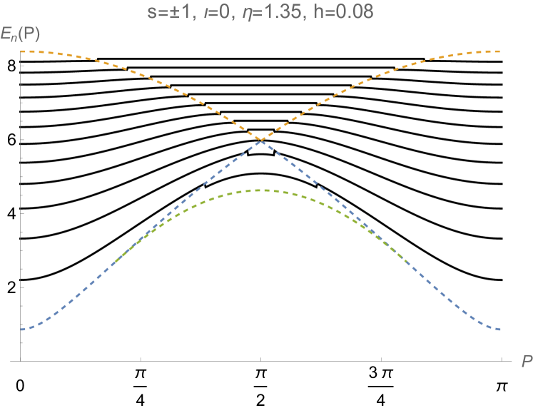
(a) Semiclassical energy spectra of the double-degenerate meson modes with spin $s=\pm 1$.

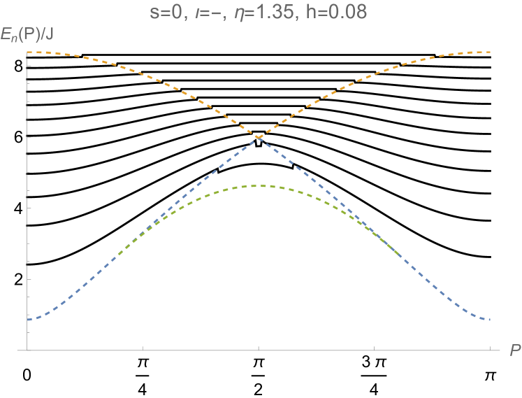
(b) Semiclassical energy spectra of the meson modes with spin $s=0$ and $\iota=-$.

Figure 12: Semiclassical energy spectra of the meson modes for the model (4) at $J=1$, $\Delta=-\cosh(1.35)$, and $h=0.08$, calculated from (275), (285), and (286).

VI.2 Low-energy regimes

Formulas (275), and (286) represent the initial terms of the semiclassical asymptotic expansions for the meson energy spectra $\tilde{E}_{\iota,n}(P)$ in integer powers of the string tension $f\to+0$. These semiclassical asymptotic expansions are supposed to work well for the meson states with large quantum numbers $n\gg 1$. For the energy spectra of mesons with small $n=1,2,\dots$, one should use instead the low-energy asymptotic expansions in fractional powers of $f$. Three such low-energy expansions were introduced in Rutkevich (2018) and discussed in Section IV.2.2 in the frame of the heuristic approach exploiting the canonical quantization of the Hamiltonian dynamics of the model (133). Now we shall describe briefly, how these low-energy expansions can be obtained in the more rigorous approach based of the perturbative solution of the Bethe-Salpeter equation (251).

As in the case of the semiclassical expansion, we start from equalities (271), and replace the integrals $J_{\beta}(\Lambda_{\iota})$ in the left-hand side by their saddle-point asymptotics at $f\to+0$. In contrast to the semiclassical regimes, however, the relevant saddle points of the function ${\mathcal{F}}(z,\Lambda_{\iota})$ in the low-energy regimes are degenerate. The kinds of the saddle-point degeneracy are different in the three low-energy regimes.

First low-energy regime.

The first low-energy regime is realised at $P\in(-P_{c}(\eta),P_{c}(\eta))$ and energies $E$ slightly above the two-kink edge $\epsilon(0|P)$. In this regime, the two Morse saddle points $z_{a}$ and $z_{a}^{-1}$ shown in Figure 18a approach with decreasing $E$ the point $z=1$, and finally merge there at $E=\epsilon(0|P)$. It is shown in Appendix D.4, that the contribution of the resulting degenerate saddle point $z=1$ into the integral $J_{1}(\Lambda_{\iota})+J_{2}(\Lambda_{\iota})$ determines the first low-energy expansion of the meson dispersion laws. The final result coincides with formula (187). This asymptotical formula holds at $f\to+0$ and $-P_{c}(\eta)<P<P_{c}(\eta)$, for not very large $n=1,2,\ldots$.

Second low-energy regime.

In the second low-energy regime, the meson momentum lies in the interval $P\in(P_{c}(\eta),\pi-P_{c}(\eta))$, and the energy is slightly above the the two-kink edge, which is given by the function $\epsilon(P,\eta)$ determined by equation (340) and plotted by the right red dashed line in Figure 10. The Morse saddle points $z_{a}$ and $z_{b}$ shown in Figure 18c merge at $E=\epsilon(P,\eta)$, as well as the saddle points $z_{a}^{-1}$ and $z_{b}^{-1}$. As the result, the small-$f$ asymptotics of the integrals $J_{1}(\Lambda_{\iota})$ and $J_{2}(\Lambda_{\iota})$ are determined in second low-energy regime by the contributions of the degenerate saddle points $\exp\left(2i\,p_{m}(P,\eta)\right)$, and $\exp\left(-2i\,p_{m}(P,\eta)\right)$, respectively, with $p_{m}(P,\eta)$ given by (340).

The calculation of these saddle-point asymptotics is described in Appendix D.5. The final result for the three initial terms in the second low-energy expansion of the meson energy spectrum reads:

$$\tilde{E}_{\iota,n}(P)=\epsilon(0|P)+f^{2/3}\left[\frac{\partial_{p}^{2}\epsilon(p|P)|_{p=p_{m}}}{2}\right]^{1/3}x_{n}-$$

$$\frac{f}{2}\partial_{p}\theta_{\iota}(P/2+p,P/2-p)\Big{|}_{p=p_{m}}+O(f^{4/3}),$$ (288)

where $x_{n}=z_{(n+1)/2}^{\prime}$ at odd $n$, $x_{n}=z_{n/2}$ at even $n$, and $n=1,2,\ldots$. Formula (288) was presented without derivation in paper Rutkevich (2018), see equation (41) there.

Third low-energy regime.

The third low-energy expansion describes the meson dispersion law close to the points $P=\pm P_{c}+\pi n$, $E=\epsilon(0|P_{c})$, with $P_{c}$ given by equation (337), and $n\in\mathbb{Z}$. These points are shown in red in Figure 10. Since $\epsilon^{\prime\prime}(0|P_{c})=0$, the Taylor expansion of the effective energy $\epsilon(p|P_{c})$ takes the form:

$$\epsilon(p|P_{c})=\epsilon(0|P_{c})+\frac{\partial_{p}^{4}\epsilon(p|P_{c})|_{p=0}}{24}p^{4}+O(p^{6}).$$ (289)

Accordingly, all four saddle points of the function $\mathcal{F}(z,\Lambda)$ given by (270) merge at $P=P_{c}$ and $\Lambda=\epsilon(0|P_{c})$:

$$z_{a}=z_{a}^{-1}=z_{b}=z_{b}^{-1}=1.$$

Derivation of the third law-energy expansion is to much extent similar to the procedure described in Appendix D.5. The main difference, however, is that the momentum and energy variables must be rescaled, instead of equations (419), in the following way:

$$p=t\,\mathfrak{p},\quad p^{\prime}=t\,\mathfrak{p}^{\prime},$$ (290a)

$$\tilde{E}_{\iota}=\epsilon(0|P_{c})+t^{4}\mathfrak{e}_{\iota},$$ (290b)

with $t=f^{1/5}$.

The final result for the third law-energy expansion reads:

$$\tilde{E}_{\iota,n}(P_{c})=\epsilon(0|P_{c})+f^{4/5}\left[\frac{\partial_{p}^{4}\epsilon(p|P_{c})|_{p=0}}{6}\right]^{1/5}c_{n}+$$

$$f\,a_{\iota}(P_{c})+O(f^{6/5}),$$ (291)

where $n=1,2,\ldots$, $a_{\iota}(P)$ is the scattering length (186), and $c_{n}$ are the consecutive solutions of equation (93) in reference Rutkevich (2008):

$$\int_{0}^{\infty}dy\,\bigg{[}\sin\bigg{(}\frac{y^{5}}{20}-y\,c_{n}\bigg{)}-\exp\bigg{(}-\frac{y^{5}}{20}+y\,c_{n}\bigg{)}\bigg{]}\cdot$$ (292)

$$\int_{0}^{\infty}dx\,x^{2}\cos\bigg{(}\frac{x^{5}}{20}-x\,c_{n}\bigg{)}=\int_{0}^{\infty}dx\,\cos\bigg{(}\frac{x^{5}}{20}-x\,c_{n}\bigg{)}\cdot$$

$$\int_{0}^{\infty}dy\,y^{2}\bigg{[}\sin\bigg{(}\frac{y^{5}}{20}-y\,c_{n}\bigg{)}+\exp\bigg{(}-\frac{y^{5}}{20}+y\ c_{n}\bigg{)}\bigg{]},$$

$c_{1}=1.787$, $c_{2}=3.544$, $c_{3}=5.086$, $c_{4}=6.518$. Note that equation (93) in paper Rutkevich (2008) contains a misprint, which is corrected in (292).

The third law-energy expansions (291) were announced in reference Rutkevich (2018), see equation (44) there.

VI.3 Crossover regimes

There are three crossover regimes, which are realized in the vicinity of the boundary curves separating the regions (I), (II) and (III) in Figure 10. In these regimes, the meson energy $E_{\iota,n}(P)$ is close to some local maximum value of the effective two-kink kinetic energy $\epsilon(p|P)$, see Figures 15 (a), (b), (c). Perturbative calculation of the meson energy spectra in these crossover regimes is based on the asymptotic saddle point analysis of the integrals $J_{\beta}(\Lambda_{\iota})$ defined in equation (272). Since these calculations are to much extent similar to those outlined above and described in Appendix D, we skip their details and present only the final results.

First crossover regime.

The first crossover regime is realised close to the boundary separating the regions (I) and (III) in Figure 10. At $P\in(P_{c}(\eta),\pi/2)$, it takes place at the meson energies $\tilde{E}_{\iota,n}(P)$ close to $\epsilon(0|P)$. At small $h\to 0$, the meson energy spectrum $\tilde{E}_{\iota,n}(P)$ is determined in this case by equations:

$$\frac{\mathrm{Ai}\,(\lambda_{\iota,n})}{\mathrm{Bi}\,(\lambda_{\iota,n})}=$$ (293)

$$\cot\left[-\frac{F(p_{a},\tilde{E}_{\iota,n}(P))}{2f}-\frac{\pi}{4}+\frac{\theta_{\iota}(P/2+p_{a},P/2-p_{a})}{2}\right],$$

with $\tilde{E}_{\iota,n}(P)=\epsilon(p_{a}|P)$, and

$$\lambda_{\iota,n}=\left(\frac{2}{f^{2}\,\left|\partial_{p}^{2}\epsilon(p,P)\right|_{p=0}}\right)^{1/3}\cdot$$ (294)

$$[\tilde{E}_{\iota,n}(P)-\epsilon(0|P)-fa_{\iota}(P)].$$

Here and below the function $F(p,E)$ is determined by (273), and $\mathrm{Bi}\,(\lambda)$ denotes the second solution

$$\mathrm{Bi}\,(\lambda)=\int_{0}^{\infty}\frac{dt}{\pi}\left[\sin\left(\frac{t^{3}}{3}+t\lambda\right)+\exp\left(-\frac{t^{3}}{3}+t\lambda\right)\right]$$ (295)

of the Airy differential equation.

Second crossover regime.

The second crossover regime is realised close to the boundary separating the regions (I) and (II) in Figure 10. At $P\in(P_{c}(\eta),\pi/2)$, it takes place at the meson energy $\tilde{E}_{\iota,n}(P)$ close to $\epsilon(\pi/2|P)$. In this case, the small-$f$ asymptotics of the meson energies $\tilde{E}_{\iota,n}(P)$ is determined by solutions of two transcendent equations:

$$\frac{\mathrm{Ai}\,(\tilde{\lambda}_{\iota,n})}{\mathrm{Bi}\,(\tilde{\lambda}_{\iota,n})}=\tan\left[\frac{F(\pi/2,\tilde{E}_{\iota,n}(P))}{2f}-\frac{\pi}{2}\,\delta_{\iota,0}\right],$$ (296)

$$\tilde{\lambda}_{\iota,n}=\left(\frac{2}{f^{2}\,\left|\partial_{p}^{2}\epsilon(p,P)\right|_{p=\pi/2}}\right)^{1/3}\cdot$$ (297)

$$\left[\tilde{E}_{\iota,n}(P)-\epsilon(\pi/2|P)+\frac{f}{2}\partial_{p}\theta_{\iota}(P/2+p,P/2-p)\Big{|}_{p=\pi/2}\right].$$

Third crossover regime.

Finally, the third crossover regime takes place at $P=\pm\pi/2+\pi n$, with $n\in\mathbb{Z}$, at energies $\tilde{E}_{\iota,n}(\pi/2)$ close $\epsilon(0|\pi/2)=\epsilon(\pi/2|\pi/2)$. These points separate the regions (II) and (III) in Figure 10, see also Figure 15b. The energy spectra $\tilde{E}_{\iota,n}(\pi/2)$ in this regime are determined by solutions of two equations:

$$\frac{[\mathrm{Bi}(\breve{\lambda}_{\iota,\iota,n})+i\,\mathrm{Ai}(\breve{\lambda}_{\iota,\iota,n})][\mathrm{Bi}(\breve{\lambda}_{\iota,-\iota,n})+i\,\mathrm{Ai}(\breve{\lambda}_{\iota,-\iota,n})]}{[\mathrm{Bi}(\breve{\lambda}_{\iota,\iota,n})-i\,\mathrm{Ai}(\breve{\lambda}_{\iota,\iota,n})][\mathrm{Bi}(\breve{\lambda}_{\iota,-\iota,n})-i\,\mathrm{Ai}(\breve{\lambda}_{\iota,-\iota,n})]}=$$

$$\exp\left[i\frac{F(\pi/2,\tilde{E}_{\iota,n}(\pi/2))}{f}-i\pi\delta_{\iota,0}\right],$$ (298)

$$\breve{\lambda}_{\iota,\iota^{\prime},n}=\left(\frac{2}{f^{2}\,\left|\partial_{p}^{2}\epsilon(p,\pi/2)\right|_{p=0}}\right)^{1/3}\cdot$$ (299)

$$\left[\tilde{E}_{\iota,n}(\pi/2)-\epsilon(0|\pi/2)-fa_{\iota^{\prime}}(\pi/2)\right],$$

where $a_{\iota}(P)$ is the scattering length (186).

Note, that due to the symmetry (132), the energy spectra $\tilde{E}_{\iota,n}(P)$ of mesons with opposite parities $\iota=\pm$ coincide at $P=\pi/2$.

VII Dynamic structure factors in the confinement regime

In this Section we describe the effect of a weak longitudinal staggered magnetic field on the structure factors of the spin operators. In the thermodynamic limit, these structure factors are defined as follows:

$$S^{\mathfrak{a}\mathfrak{b}}(\mathrm{k},\omega|h)=\frac{1}{8}\sum_{j=-\infty}^{\infty}e^{-i\mathrm{k}j}\int_{-\infty}^{\infty}dt\,e^{i\omega t}\cdot$$ (300)

$$\Big{[}\langle vac(h)|\sigma_{j}^{\mathfrak{a}}(t)\sigma_{0}^{\mathfrak{b}}(0)|vac(h)\rangle+$$

$$\langle vac(h)|\sigma_{j+1}^{\mathfrak{a}}(t)\sigma_{1}^{\mathfrak{b}}(0)|vac(h)\rangle\Big{]},$$

where $|vac(h)\rangle$ is the ground state of the infinite spin chain with the Hamiltonian (4). As in Section III, we shall limit our attention to the case $\mathrm{k}\in(0,\pi)$ without loss of generality.

Two approximations will be used in calculation of the structure factors (300). First, the analysis will be limited to the leading order in the weak staggered magnetic field $h$. In accordance with equation (121), this allows one to replace the vacuum state $|vac(h)\rangle$ in equation (300) by its zero-field counterpart $|vac\rangle^{(1)}$. Second, as in Section III, the analysis will be restricted solely to the two-spinon contribution to the structure factor. In the leading order in $h$, the latter is given by equation (96). The operator $\mathcal{P}_{11}^{(2)}$ in this equation denotes the projector onto the two-kink subspace $\mathcal{L}_{11}^{(2)}$. This projector operator admits representation (51b) in terms of the two-kink basis states $|K_{10}(p_{1})K_{01}(p_{2})\rangle_{s_{1}s_{2}}$. However, since such two-kink states do not diagonalize the Hamiltonian (4) at any non-zero staggered magnetic field $h$, representation (51b) of the operator $\mathcal{P}_{11}^{(2)}$ cannot be used for calculation of the DSF (96) at $h>0$. Instead, we shall use the following expansion of this projector operator in the basis of meson states $|\tilde{\pi}_{s,\iota}(P)\rangle$ determined by equations (197), (199), and (200):

$$\mathcal{P}_{11}^{(2)}=\sum_{s=0,\pm 1}\mathcal{P}_{s}^{(2)}.$$ (301)

Here

$$\mathcal{P}_{s}^{(2)}=\int_{0}^{\pi}\frac{dP}{\pi}\sum_{n=1}^{\infty}|\tilde{\pi}_{s,\iota=0,n}(P)\rangle\langle\tilde{\pi}_{s,\iota=0,n}(P)|$$ (302)

for $s=\pm 1$, and

$$\mathcal{P}_{s=0}^{(2)}=\mathcal{P}_{s=0,\iota=+}^{(2)}+\mathcal{P}_{s=0,\iota=-}^{(2)},$$ (303)

$$\mathcal{P}_{s=0,\iota}^{(2)}=\int_{0}^{\pi}\frac{dP}{\pi}\sum_{n=1}^{\infty}|\tilde{\pi}_{s=0,\iota,n}(P)\rangle\langle\tilde{\pi}_{s=0,\iota,n}(P)|.$$

VII.1 Transverse DSF

Formulas (96), (301), (302) lead in the adopted approximation to the following representation for the transverse DSF:

$$S_{(2)}^{+-}(\mathrm{k},\omega|h)=\frac{1}{8}\sum_{j=-\infty}^{\infty}e^{-i\mathrm{k}j}\int_{-\infty}^{\infty}dt\,e^{i\omega t}\cdot$$ (304)

$$\Big{[}\phantom{.}^{(1)}\langle vac|\sigma_{j}^{+}(t)\mathcal{P}_{s=-1}^{(2)}\sigma_{0}^{-}(0)|vac\rangle^{(1)}+$$

$$\phantom{.}{}^{(1)}\langle vac|\sigma_{j+1}^{+}(t)\mathcal{P}_{s=-1}^{(2)}\sigma_{1}^{-}(0)|vac\rangle^{(1)}\Big{]}.$$

Integration in $t$ and summation in $j$ in the right-hand side can be performed using equations (125a), (126), and following the procedure described in Section III. The result reads:

$$S_{(2)}^{+-}(\mathrm{k},\omega|h)=\sum_{n=1}^{\infty}\delta[\omega-\tilde{E}_{\iota=0,n}(P)]\,I_{n}^{+-}(P|h)\Big{|}_{P=\mathrm{k}},$$ (305)

where $\tilde{E}_{\iota=0,n}(P)$ is the dispersion law of two degenerate meson modes with $\iota=0$ and $s=\pm 1$ in the two-kink approximation, and $I_{n}^{+-}(P|h)$ are the intensities corresponding to these modes:

$$I_{n}^{+-}(P|h)=\frac{\pi}{4}\,\big{|}\phantom{.}^{(1)}\langle vac|\sigma_{0}^{+}|\tilde{\pi}_{s=-1,\iota=0,n}(P)\rangle+$$ (306)

$$\phantom{.}{}^{(1)}\langle vac|\sigma_{0}^{-}|\tilde{\pi}_{s=1,\iota=0,n}(P)\rangle\big{|}^{2}.$$

The matrix elements of the $\sigma_{0}^{\pm}$ operators in the right-hand side can be expressed in terms of the wave function $\phi_{\iota=0,n}(p|P)$ solving the Bethe-Salpeter equation (218) and normalized by the condition (231):

$$\phantom{.}^{(1)}\!\langle vac|\sigma_{0}^{\pm}|\tilde{\pi}_{s=\mp 1,\iota=0,n}(P)\rangle=\int_{0}^{\pi/2}\frac{dp}{\pi}\,\phi_{\iota=0,n}(p|P)e^{-i(p+P/2)}\phantom{.}{}^{(1)}\!\langle vac|\sigma_{0}^{\pm}|K_{10}(P/2+p)K_{01}(P/2-p)\rangle_{\mp 1/2,\mp 1/2}.$$ (307)

The matrix elements of the $\sigma_{0}^{\pm}$ operators between the vacuum and two-kink states are, in turn, simply related due to (59), (73a), (73b) with the form factors $X^{1}(\xi_{1},\xi_{2})$ and $X^{0}(\xi_{1},\xi_{2})$ given by equation (75).

Thus, equations (305) - (307) describe the transverse DSF in the antiferromagnetic XXZ spin chain in the confinement regime in the two-kink approximation. Substitution of obtained in Section VI perturbative solutions of the Bethe-Salpeter equation (218) instead of the wave function $\phi_{\iota=0,n}(p|P)$ in the right-hand side of (307) yields the explicit asymptotical formulas for the transverse DSF in the limit $h\to+0$. In what follows, we shall restrict our analysis to the semiclassical approximations for the meson wave function, which were described in Section VI.1.

In the semiclassical regimes, the wave function $\phi_{\iota=0,n}(p|P)$ becomes highly oscillating in $p$ at $h\to 0$, while the matrix element in the integrand in the right-hand side of (307) remains regular and smooth in this limit. As the result, the semiclassical asymptotics of the integral in the right-hand side of (307) is determined by contributions of the saddle points, which are located at the solutions of the equation

$$\epsilon(p|P)=\tilde{E}_{n}(P).$$ (308)

VII.1.1 First semiclassical regime

There is only one such saddle point $p=p_{a}$ in the interval $(0,\pi/2)$ in the first semiclassical regime at $0<P<P_{c}(\eta)$. Accordingly, in the leading order in $h\to 0$, we can apply the asymptotical formula (402) for the function $\phi_{\iota=0,n}(p|P)$ and then perform integration in $p$ in the right-hand side of (307) using the Dirac delta-function $\delta(p-p_{a})$. As the result, we obtain in this case:

$$I_{n}^{+-}(P|h)=\frac{\pi f}{p_{a}}\,S_{(2)}^{+-}(P,\omega|0)\Big{|}_{\omega=\tilde{E}_{n}(P)},$$ (309)

where $S_{(2)}^{+-}(P,\omega|0)$ is the two-kink contribution to the transverse DSF at zero staggered magnetic field given by equation (106).

The result (309) for the intensity $I_{n}^{+-}(P|h)$ holds in the first semiclassical regime at $0<P<P_{c}(\eta)$. On the other hand, at $\pi-P_{c}(\eta)<P<\pi$ and $\epsilon(\pi/2|P)<\tilde{E}_{n}(P)<\epsilon(0|P)$, the unique solution of equation (308) in the interval $(0,\pi/2)$ is $p=p_{b}$. In this case, we obtain instead of (309):

$$I_{n}^{+-}(P|h)=\frac{\pi f}{\pi/2-p_{b}}\,S_{(2)}^{+-}(P,\omega|0)\Big{|}_{\omega=\tilde{E}_{n}(P)}.$$ (310)

It is instructive to rewrite (309), (310) in the equivalent form:

$$I_{n}^{+-}(P|h)=\Delta{E}_{n}^{(\mathrm{I})}(P)\,\cdot S_{(2)}^{+-}(P,\omega|0)\Big{|}_{\omega=\tilde{E}_{n}(P)},$$ (311)

where

$$\Delta{E}_{n}^{(\mathrm{I})}(P)\equiv\tilde{E}_{\iota,n+1}(P)-\tilde{E}_{\iota,n}(P)=$$ (312)

$$\begin{cases}\frac{\pi f}{p_{a}}+O(f^{2}),&0<P<P_{c}(\eta),\\ \frac{\pi f}{\pi/2-p_{b}}+O(f^{2}),&\pi-P_{c}(\eta)<P<\pi\end{cases}$$

is the small interval between two sequential energies of the $\iota$-meson mode at given $P$ in the first semiclassical regime.

Let us sum both sides of equality (311) in $n$ at some fixed $P\in(0,P_{c}(\eta))$:

$$\sum_{n=1}^{\mathcal{N}(P|h)}I_{n}^{+-}(P|h)=\sum_{n=1}^{\mathcal{N}(P|h)}\Delta{E}_{n}^{(\mathrm{I})}(P)\,S_{(2)}^{+-}(P,E|0)),$$ (313)

where the upper limit of summation $\mathcal{N}(P|h)$ is given by equation (277). Due to (305), we have in the left-hand side the integral

$$\int_{\epsilon(0|P)}^{\epsilon(\pi/2|P)}dE\,S_{(2)}^{+-}(P,E|h),$$ (314)

while the right-hand side of (313) represents the Riemann sum approximating at small $f$ the integral

$$\int_{\epsilon(0|P)}^{\epsilon(\pi/2|P)}dE\,S_{(2)}^{+-}(P,E|0).$$ (315)

The function $S_{(2)}^{+-}(P,E|0)$ vanishes at energies $E$ outside the interval $(\epsilon(0|P),\epsilon(\pi/2|P))$, as well as the function $S_{(2)}^{+-}(P,E|h)$ at $h\to 0$. Thus, we obtain from (313):

$$\lim_{h\to+0}\int_{0}^{\infty}dE\,S_{(2)}^{+-}(P,E|h)=\int_{0}^{\infty}dE\,S_{(2)}^{+-}(P,E|0).$$ (316)

Despite the confinement of kinks induced by the arbitrary weak staggered magnetic field $h>0$, the two-kink transverse DSF integrated over the energy is continuous in $h$ at $h\to+0$.

VII.1.2 Third semiclassical regime

There are two saddle points $p_{b}<p_{a}$ in the interval $(0,\pi/2)$ in the third semiclassical regime at $P\in(P_{c}(\eta),\pi-P_{c}(\eta))$. To the leading order in $h$, the reduced meson wave function $\phi_{0,n}(p|P)$ is determined by equations (404), (409), and (252). The delta-functions in the right-hand side of (404) give rise to two terms after integration in $p$ in the right-hand side of (307). Then, substitution of the result in (306) and subsequent straightforward calculations yield:

$$I_{n}^{+-}(P|h)=\Delta{E}_{n}^{(\mathrm{III})}\Big{[}S_{(2)}^{+-}(P,\omega|0)+Z_{n}^{+-}(P,\omega)\Big{]}\Big{|}_{\omega=\tilde{E}_{n}(P)},$$ (317)

where $\Delta{E}_{n}^{(\mathrm{III})}$ is given by (287), $S_{(2)}^{+-}(P,\omega|0)$ is the transverse DSF at zero magnetic field given by (106), and the oscillating in $n$ term

$$Z_{n}^{+-}(P,\omega)\!=\!\frac{(-1)^{n-1}\,J^{2}\sinh^{2}\eta}{2[|\epsilon^{\prime}(p_{a})\,\epsilon^{\prime}(p_{b})|\,\omega(p_{1a})\omega(p_{2a})\omega(p_{1b})\omega(p_{2b})]^{1/2}}\cdot$$

$$\mathrm{Re}\bigg{\{}\left[X^{1}(\xi_{1a},\xi_{2a})+X^{0}(\xi_{1a},\xi_{2a})\right]\cdot$$ (318)

$$\left[X^{1}(\xi_{1b},\xi_{2b})+X^{0}(\xi_{1b},\xi_{2b})\right]^{*}\cdot$$

$$\exp\left[\frac{i}{2}[\theta_{0}(p_{1b},p_{2b})-\theta_{0}(p_{1a},p_{2a})]\right]\bigg{\}},$$

results from the interference of contributions of two saddle points $p_{a}$ and $p_{b}$. In equation (318), we have used notations (148), and (161).

VII.2 Longitudinal DSF

The longitudinal DSF $S_{(2)}^{zz}(\mathrm{k},\omega|h)$ in the weak confinement regime in the adopted approximation is given by equation (96), in which the projection operator $\mathcal{P}_{11}^{(2)}$ is replaced by the operator $\mathcal{P}_{s=0}^{(2)}$ given by (303), and $\mathfrak{a}=\mathfrak{b}=z$. Exploiting equalities (11), (23), and (127), equation (96) can be then simplified to the form:

$$S_{(2)}^{zz}(\mathrm{k},\omega|h)=\sum_{j=-\infty}^{\infty}\frac{e^{-i\mathrm{k}j}}{4}\,\int_{-\infty}^{\infty}dt\,e^{i\omega t}\cdot$$ (319)

$$\phantom{.}{}^{(1)}\langle vac|\sigma_{j}^{z}(t)\mathcal{P}_{s=0}^{(2)}\sigma_{0}^{z}(0)|vac\rangle^{(1)}.$$

The summation in the right-hand side should be performed separately for even, and for odd $j$. Denoting corresponding partial sums as $\Sigma_{even}$ and $\Sigma_{odd}$, respectively, we obtain after straightforward calculations exploiting equalities (11), (21), (199a), and (199b):

$$\Sigma_{even}=\frac{1}{2}\int_{0}^{\pi}dP\!\!\sum_{m=-\infty}^{\infty}e^{2mi(P-\mathrm{k})}\cdot$$ (320)

$$\sum_{\iota=\pm}\sum_{n=1}^{\infty}\delta\left[\omega-\tilde{E}_{\iota,n}(P)\right]\left|\phantom{.}{}^{(1)}\langle vac|\sigma_{0}^{z}|\tilde{\pi}_{s=0,\iota,n}(P)\rangle\right|^{2},$$

$$\Sigma_{odd}=\frac{1}{2}\int_{0}^{\pi}dP\sum_{m=-\infty}^{\infty}e^{2mi(P-\mathrm{k})}\sum_{\iota=\pm}(-\iota)\cdot$$ (321)

$$e^{i(P-\mathrm{k})}\sum_{n=1}^{\infty}\delta\left[\omega-\tilde{E}_{\iota,n}(P)\right]\left|\phantom{.}{}^{(1)}\langle vac|\sigma_{0}^{z}|\tilde{\pi}_{s=0,\iota,n}(P)\rangle\right|^{2},$$

with

$$S_{(2)}^{zz}(\mathrm{k},\omega|h)=\Sigma_{even}+\Sigma_{odd}.$$ (322)

Using the Poisson summation formula (100), and assuming that $0<\mathrm{k}<\pi$, formulas (320), (321) can be simplified to the form:

$$\Sigma_{even}=\frac{1}{2}\sum_{\iota=\pm}\sum_{n=1}^{\infty}\delta\left[\omega-\tilde{E}_{\iota,n}(P)\right]\,I_{\iota,n}^{zz}(P|h)\Big{|}_{P=\mathrm{k}},$$ (323)

$$\Sigma_{odd}=\frac{1}{2}\sum_{\iota=\pm}(-\iota)\sum_{n=1}^{\infty}\delta\left[\omega-\tilde{E}_{\iota,n}(P)\right]\,I_{\iota,n}^{zz}(P|h)\Big{|}_{P=\mathrm{k}},$$ (324)

where

$$I_{\iota,n}^{zz}(P|h)=\pi\,\left|\phantom{.}{}^{(1)}\langle vac|\sigma_{0}^{z}|\tilde{\pi}_{s=0,\iota,n}(P)\rangle\right|^{2}.$$ (325)

Adding (323) and (324), we get finally:

$$S_{(2)}^{zz}(\mathrm{k},\omega|h)=\sum_{n=1}^{\infty}\delta[\omega-\tilde{E}_{\iota,n}(P)]\,I_{\iota,n}^{zz}(P|h)\Big{|}_{\begin{smallmatrix}P=\mathrm{k}\\ \iota=-\end{smallmatrix}}.$$ (326)

Note, that the meson states with $s=0$, $\iota=+$ do not contribute to the longitudinal structure factor $S_{(2)}^{zz}(\mathrm{k},\omega|h)$: the quantum interference leads to the mutual cancellation of contributions of two magnetic sub-lattices of the antiferromagnetic ground state $|vac\rangle^{(1)}$.

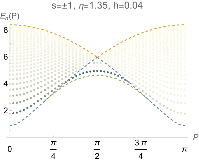
(a) Transverse modes with $s=\pm 1$.

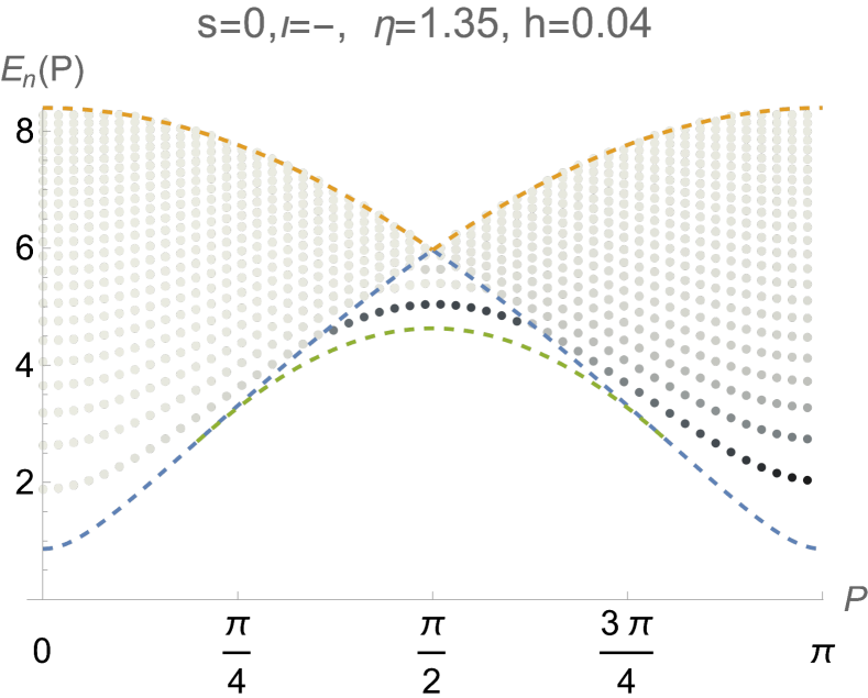
(b) Longitudinal modes modes with $s=0$, $\iota=-$.

Figure 13: Semiclassical energy spectra of the transverse (a) and longitudinal (b) meson modes at $\eta=1.35$, $h=0.04$. Darkness of the dotts characterizes the intensities of the meson modes. Dashed lines are the same as in Figure 12.

The matrix element of the $\sigma_{0}^{z}$ operator in the right-hand side of (325) can be expressed in terms of the wave function $\phi_{\iota=-,n}(p|P)$ solving equation (218) and satisfying the normalisation condition (231):

$$\phantom{.}{}^{(1)}\!\langle vac|\sigma_{0}^{z}|\tilde{\pi}_{s=0,\iota=-,n}(P)\rangle=\int_{0}^{\pi/2}\frac{dp}{\pi}\,\phi_{\iota=-,n}(p|P)\cdot$$

$$\phantom{.}{}^{(1)}\!\langle vac|\sigma_{0}^{z}|K_{10}(P/2+p)K_{01}(P/2-p)\rangle_{-}.$$ (327)

As in the previous Section VII.1, we restrict our analysis to the calculation of the semiclassical small-$h$ asymptotics of the DSF. These calculations for the longitudinal DSF are very similar to those described in Section VII.1, but now they are based on equations (325)-(327), instead of (305)-(307). Skipping the details of these calculations, we present below only the final results.

In the first semiclassical regime, the function $I_{\iota=-,n}^{zz}(P|h)$ reads:

$$I_{\iota=-,n}^{zz}(P|h)=\Delta{E}_{n}^{(\mathrm{I})}(P)\cdot S_{(2)}^{zz}(P,\omega|0)\Big{|}_{\omega=\tilde{E}_{n}(P)},$$ (328)

and $S_{(2)}^{zz}(P,\omega|0)$ is the longitudinal DSF at $h=0$ given by equation (116). The latter simplifies in the first semiclassical region to the form:

$$S_{(2)}^{zz}(P,\omega|0)=\frac{\mathcal{G}_{0}^{zz}(P/2+p,P/2-p)}{|\partial_{p}\epsilon(p|P)|}\Bigg{|}_{p=p_{0}},$$ (329)

where $p_{0}=p_{a}$ at $P\in(0,P_{c}(\eta))$, $p_{0}=p_{b}$ at $P\in(\pi/2,\pi-P_{c}(\eta))$, and $\mathcal{G}_{0}^{zz}(p_{1},p_{2})$ is determined by (115).

In the third semiclassical regime

$$I_{\iota=-,n}^{zz}(P|h)=\Delta{E}_{n}^{(\mathrm{III})}\Big{[}S_{(2)}^{zz}(P,\omega|0)+Z_{n}^{zz}(P,\omega)\Big{]}\Big{|}_{\omega=\tilde{E}_{n}(P)},$$ (330)

where $\Delta{E}_{n}^{(\mathrm{III})}$ and $S_{(2)}^{+-}(P,\omega|0)$ are given by equations (287), and (116), respectively, and the oscillating in $n$ term reads:

$$Z_{n}^{zz}(P,\omega)\!=\!\frac{(-1)^{n-1}\,2\,J^{2}\sinh^{2}\eta}{[\left|\epsilon^{\prime}(p_{a})\,\epsilon^{\prime}(p_{b})\right|\,\omega(p_{1a})\omega(p_{2a})\omega(p_{1b})\omega(p_{2b})]^{1/2}}\cdot$$

$$\mathrm{Re}\bigg{\{}X_{-}^{z}(\xi_{1a},\xi_{2a})\left[X_{-}^{z}(\xi_{1b},\xi_{2b})\right]^{*}\cdot$$ (331)

$$\exp\left[\frac{i}{2}[\theta_{-}(p_{1b},p_{2b})-\theta_{-}(p_{1a},p_{2a})]\right]\bigg{\}}.$$

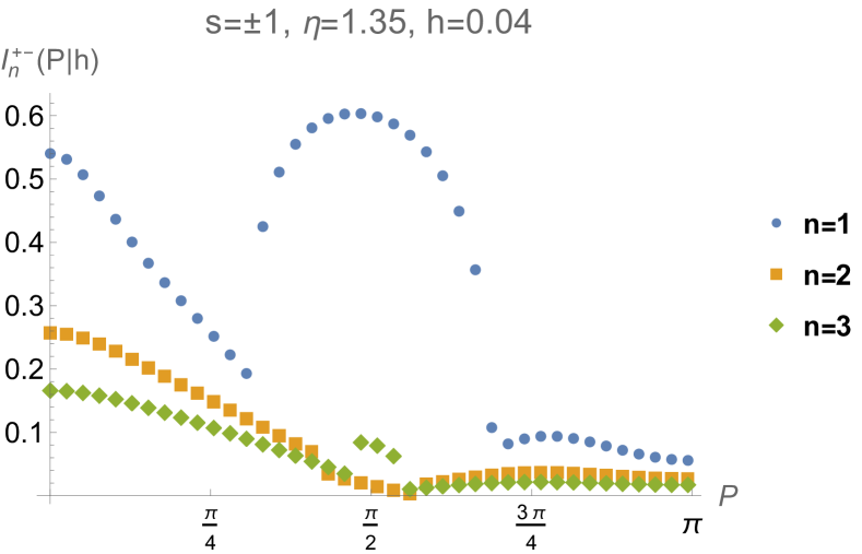
(a) Intensities $I_{n}^{+-}(P|h)$ of the transverse modes with $s=\pm 1$.

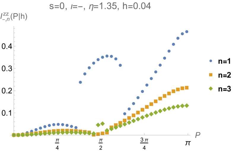
(b) Intensities $I_{-,n}^{zz}(P|h)$ of the longitudinal modes with $s=0$, $\iota=-$.

Figure 14: Momentum dependences of intensities of three lowest meson modes at $\eta=1.35$, $h=0.04$.

.

The obtained results are illustrated in Figure 13. It displays the similar semiclassical meson energy spectra determined by equations (275), (286), and (132) at $\eta=1.35$, as those in Figure 12, but at the smaller value of the magnetic field $h=0.04$. The dispersion curves for the two degenerate meson modes with $s=\pm 1$ plotted in Figure 13a, and Figure 13b show the energy spectra of the modes with $s=0$ and $\iota=-$. The darkness of the points in Figure 13 characterizes the intensities of the corresponding modes. For the transverse modes shown in Figure 13a, these intensities are determined by equations (311), (325), while for the longitudinal modes with $s=0$ and $\iota=-$ shown in Figure 13b, the intensities are given by equations (328), (330). The DSF intensities of the $s=0$ meson modes with $\iota=+$ are equal to zero.

The intensities of the meson dispersion curves in Figure 13 display very different qualitative behaviour in three regions of the $(PE)$-plane shown in Figure 10. In the first regions (I), the intensities $I_{n}^{+-}(P|h)$ and $I_{-,n}^{zz}(P|h)$ monotonically decrease with increasing $n$. In the third region (III), the dependence of the intensities is non-monotonic and alternating in $n$. In the second region (II), the intensities vanish in the adopted two-spinon semiclassical approximation.

These features of the meson DSF are clearly seen in Figure 14 showing rather peculiar momentum dependencies of intensities of three lowest transverse (Figure 14a) and longitudinal (Figure 14b) meson modes.

VIII Conclusions

We have investigated the main properties of the spinon bound-state (“meson”) excitations in the infinite XXZ spin chain in the massive antiferromagnetic phase in the weak confinement regime, which takes place in this model in the presence of a weak staggered longitudinal magnetic field $h$. We analytically calculated the small-$h$ asymptotics of the meson energy spectra in the whole Brillouin zone using two different perturbative schemes. In the first, less rigorous, but more physically transparent approach, the meson energy spectra were obtained by quantization of the Hamiltonian dynamics of two classical particles moving along the line and attracting one another with a linear potential. The results for the meson energy spectra obtained this way were confirmed and extended by means of a more rigorous and systematic technique exploiting the perturbative solution of the Bethe-Salpeter integral equation (256), which was derived for the XXZ spin-chain model (4) in Section V. Based on this perturbative analysis, we have described nine asymptotic regimes, which are realized in different regions of the meson energy-momentum plane. A similar structure of the meson energy spectra in the weak confinement regime was previously found Rutkevich (2008) in the Ising spin-chain model (34) perturbed by a weak uniform longitudinal magnetic field. This is not surprising, since the kink dispersion laws in models (5) and (34) are the same up to a re-parametrization. Finally, using the perturbative solution of the Bethe-Salpeter equation, explicit formulas were obtained for the two-kink contribution to the transverse and longitudinal dynamical structure factors of the local spin operators for the XXZ spin chain model in the weak confinement regime.

Strictly speaking, nine asymptotic expansions, the initial terms of which are presented in Section VI, describe in model (4) the small-$h$ asymptotic behavior of the meson energy spectra in the whole Brillouin zone. We expect, however, that a rather accurate numerical description of all meson energy spectra at small $h$ can be provided solely by the three semiclassical expansions (275), (285), and (286). This suggests, in particular, that the semiclassical formulas can be used not only to describe the energy spectra of mesons with large quantum number $n\gg 1$, but may also work well for lowest lying mesons with $n=1,2,\ldots$. The high efficiency of the semiclassical formulas for description of the energy spectra of light mesons in different QFT and spin-chain models exhibiting confinement was confirmed in various works Lencsés and Takács (2015); Kormos et al. (2017); Lagnese et al. (2020); Lencsés et al. (2022).

We believe that, even though the energy spectra of magnetic excitations can be determined by direct numerical methods, such as the DMRG, the matrix product state (MPS) approach, and other techniques, the analytically obtained in this paper formulas for the meson energy spectra and the magnetic DSFs will be helpful for understanding and interpretation of the results on the inelastic neutron-scattering and terahertz spectroscopy experiments in quasi-1D antiferromagnetic crystals in the confinement regime.

The main advantage of our analytic approach is that, in contrast to the direct numerical methods that typically require considerable computational time and efforts in order to determine the magnetic excitation energy and DSF at certain fixed values of the model parameters and quasi-momentum, the analytic perturbative techniques developed in this paper provide explicit formulas for these quantities in the whole Brillouin zone in a wide range of parameters $\Delta$ and $h$. This allows us, in particular, to predict the non-monotonic $n$-dependence of the DSF at wave-vectors $\mathrm{k}$ close to $\pi/2$, see Figures 13, and 14, and to elucidate the non-trivial role of the elastic two-spinon scattering in forming the meson energy spectra in the semiclassical and low-energy regimes, see equations (172), (187), (286), and (288).

There are several directions for further study. The procedure developed in Section V can be applied to a derivation of the Bethe-Salpeter equation in other QFTs and spin-chain models exhibiting confinement, which are integrable, but not free in the deconfined phase.

For experimental applications, it would be interesting to extend the analysis of the spinon confinement in the XXZ spin-chain model (4) to the case of nonzero temperatures. It would be also interesting to study theoretically the effect of a uniform transverse magnetic field on the spinon confinement in this model.

Appendix A Properties of the function $\epsilon(p|P)$

In this Appendix we describe in details the properties of the ”kinetic energy of two spinons in the center momentum frame”

$$\epsilon(p|P)=\omega(P/2+p)+\omega(P/2-p),$$ (332)

where $\omega(p)$ is the spinon dispersion law (30).

The symmetry properties of this function

$$\epsilon(p|P)=\epsilon(p+\pi|P)=\epsilon(-p|P)=\epsilon(p|-P),$$ (333)

$$\epsilon(p|P)=\epsilon(p+\pi/2|-P+\pi),$$ (334)

$$\epsilon(p|\pi/2)=\epsilon(p+\pi/2|\pi/2)=\epsilon(-p+\pi/2|\pi/2).$$ (335)

follow immediately from its definition.

(a) $0\leq P<\pi/2$

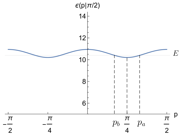
(b) $P=\pi/2$

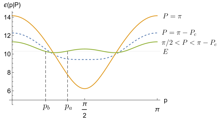
(c) $\pi/2<P\leq\pi$

Figure 15: Energy of two spinons $\epsilon(p|P)$ defined by (332) at different $P$ as the function of $p$ at $\eta=\mathrm{arccosh}\,5$. The critical momentum $P_{c}(\eta)$ is determined by (337).

.

Evolution of the $p$-dependence of the function $\epsilon(p|P)$ with increasing $P\in[0,\pi]$ is shown in Figure 15. At $P=0$, the function $\epsilon(p|P)$ takes the minimum value at $p=0$, and monotonically increases with increasing $p$ in the interval $0\leq p\leq\pi/2$, see Figure 15a. This qualitative behavior of the $p$-dependence of the function $\epsilon(p|P)$ does not change with increasing $P$ until the latter reaches the critical value $P_{c}(\eta)$ determined by the conditions

$$\partial_{p}^{2}\epsilon(p|P_{c})\Big{|}_{p=0}=0,\quad 0<P_{c}<\pi/2.$$ (336)

The critical total momentum $P_{c}(\eta)$ can be represented in terms of the complementary elliptic modulus $k^{\prime}(\eta)$

$$P_{c}(\eta)=\mathrm{arccos}\,\frac{1-k^{\prime}(\eta)}{1+k^{\prime}(\eta)},$$ (337)

which in turn can be expressed as the squared ratio of two elliptic theta-functions (83):

$$k^{\prime}(\eta)=\left(\frac{\vartheta_{4}(0,e^{-\eta})}{\vartheta_{3}(0,e^{-\eta})}\right)^{2}=\left(\frac{\vartheta_{2}(0,e^{-\pi^{2}/\eta})}{\vartheta_{3}(0,e^{-\pi^{2}/\eta})}\right)^{2}.$$ (338)

At larger $P$ in the interval $P_{c}(\eta)<P<\pi/2$, the function $\epsilon(p|P)$ becomes non-monotonic in $p$ at $0<p<\pi/2$. It has a local maximum at $p=0$, and takes the minimum value $\epsilon_{m}$ at $p=p_{m}\in(0,\pi/4)$, where

$$\epsilon_{m}(P,\eta)=I(\eta)\,[1+k^{\prime}(\eta)]\,\sin P,$$ (339)

$$p_{m}(P,\eta)=\frac{1}{2}\,\mathrm{arccos}\left(\,\frac{\cos P}{\cos P_{c}(\eta)}\right).$$ (340)

Here the constant $I(\eta)$ is determined by (31).

The $p$-dependence of the function $\epsilon(p,P)$ at $P=\pi/2$ is shown in Figure 15b. The additional symmetries (335) holding at $P=\pi/2$ lead to the following equalities:

$$\epsilon(0,\pi/2)=\epsilon(\pi/2,\pi/2),\quad p_{m}(\pi/2,\eta)=\pi/4.$$ (341)

Finally, Figure 15c displays the $p$-dependence of the function $\epsilon(p|P)$ at $\pi/2<P\leq\pi$. Due to the symmetry (334), the curves on this Figure are shifted to the right by $\pi/2$ with respect to their counterparts in Figure 15a.

As one can see from Figure 15, the number $\mathfrak{N}(P,\omega)$ of real solutions $p^{(i)}\in(0,\pi/2)$ of the equation $\epsilon(p|P)=\omega$ for $P\in(0,\pi)$, and $\omega$ in the kinematically allowed interval (107), is the following:

$$\mathfrak{N}(P,\omega)=\begin{cases}2,&P_{c}(\eta)<P\leq\pi/2,\quad\quad\;\;\;\omega<\epsilon(0,P),\\ 2,&\pi/2<P<\pi-P_{c}(\eta),\quad\omega<\epsilon(\pi/2,P),\\ 1,&\text{otherwise}.\end{cases}$$ (342)

To describe the properties of the function $\epsilon(p|P)$ analytically continued into the complex $p$-plane, we proceed to the variables:

$$z=e^{2ip},\quad v=e^{iP},\quad\mathfrak{h}=\frac{1-k^{\prime}}{1+k^{\prime}}.$$ (343)

Due to (338), the parameter $\mathfrak{h}$ depends on $\eta$, and varies in the interval $(0,1)$ at $\eta\in(0,\infty)$, see Figure 16. In new variables (343), the function $\epsilon(p|P)$ can be written as:

$$\epsilon(p|P)=\mathcal{E}(z|v)=\frac{Ik}{2}\,\Omega(z),$$ (344)

where

$$\Omega(z)=\left(\mathfrak{h}+\frac{1}{\mathfrak{h}}-\frac{z}{v}-\frac{v}{z}\right)^{1/2}+\left(\mathfrak{h}+\frac{1}{\mathfrak{h}}-{v}{z}-\frac{1}{zv}\right)^{1/2}.$$ (345)

Note, that the function $\mathcal{E}(z|v)$ stands in the left-hand side of the Bethe-Salpeter equation (256).

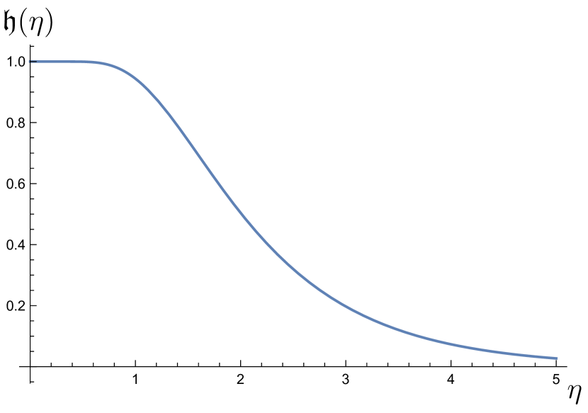
Figure 16: Variation of the parameter $\mathfrak{h}$ determined by (343) and (338) with $\eta$.

The algebraic function $\Omega(z)$ has in the complex plane six square-root branching points:

$$0,\,\mathfrak{h}v,\,\mathfrak{h}v^{-1},\,\mathfrak{h}^{-1}v,\,\mathfrak{h}^{-1}v^{-1},\,\infty.$$ (346)

Its Riemann surface $\mathfrak{L}$ has four sheets $\mathfrak{L}_{\alpha\beta}$ with $\alpha,\beta=\pm 1$, which are distinguished by the signs of the first and the second terms in the right-hand side of (345) at $z=1$.

Figure 17: Branching points of function $\Omega(z)$ determined by (345), and cuts on $z$-plane for $|v|=1$, and $\mathfrak{h}\in(0,1)$.

As in Rutkevich (2008), we draw four cuts on the $z$-plane shown in Figure 17, in order to separate these sheets. The sheet $\mathfrak{L}_{++}$ will be called ”the physical sheet”.

Note, that for $v=e^{iP}$ with $0<P<\pi$ and real $\mathfrak{h}$, the function $\Omega(z)$ has in the physical sheet the following asymptotical behavior at real $z\to 0$:

$$\Omega(z)=\begin{cases}{2{z^{-1/2}}\sin\frac{P}{2}}+O(z^{1/2}),&\text{if }z>0,\\ {2{|z|^{-1/2}}\cos\frac{P}{2}}+O(|z|^{1/2}),&\text{if }z<0.\end{cases}$$ (347)

The equation

$$\Omega(z)=\lambda$$ (348)

has four solutions $z_{a},z_{a}^{-1},z_{b},z_{b}^{-1}$ in the Riemann surface $\mathfrak{L}$, which are given by

$$z_{\alpha}+z_{\alpha}^{-1}=-\frac{v+v^{-1}}{(v-v^{-1})^{2}}\lambda^{2}\mp$$ (349)

$$2\left[1+\frac{(\mathfrak{h}+\mathfrak{h}^{-1})\lambda^{2}}{(v-v^{-1})^{2}}+\frac{\lambda^{4}}{(v-v^{-1})^{4}}\right]^{1/2},$$

with $\alpha=a,b$. At certain values of parameters $v,\mathfrak{h}$ the point $z_{a}$, or $z_{b}$, or both of them, lie in the unit circle $|z|=1$. In this case, the corresponding solution of equation (108) can be recovered from (343), (344) and (349):

$$p_{a,b}(P,\omega)=\frac{1}{2}\mathrm{arccos}\,\Bigg{\{}\left(\frac{\omega}{I\,k\sin P}\right)^{2}{\cos P}\,\mp$$ (350)

$$\sqrt{\left[1-\left(\frac{\omega}{I\,(1-k^{\prime})\sin P}\right)^{2}\right]\left[1-\left(\frac{\omega}{I\,(1+k^{\prime})\sin P}\right)^{2}\right]}\Bigg{\}}.$$

Appendix B Form factors of the $\sigma_{0}^{z}$ operator

The form factors of the $\sigma_{0}^{z}$ operator are defined as the matrix element between the $\mu$-th vacuum and the $n$-kink state with even $n$:

$$f^{\mu}(\alpha_{1},\ldots,\alpha_{n})_{s_{1},\ldots,s_{n}}=$$ (351)

$$\phantom{.}{}^{(\mu_{1})}\langle vac|\sigma_{0}^{z}|\mathcal{K}_{\mu_{n+1}\mu_{n}}(\xi_{n})\ldots\mathcal{K}_{\mu_{2}\mu_{1}}(\xi_{1})\rangle_{s_{n},\ldots,s_{1}},$$

where $\mu_{1}=\mu_{n+1}=\mu$, and $\xi_{j}=-ie^{i\alpha_{j}}$. For indices $\mu\in\{0,1\}$, we shall use the following notations: $\overline{0}=1$, $\overline{1}=0$. Since $\mu_{j+1}=\overline{\mu_{j}}$, we have $\mu_{j}=\mu_{1}$ for odd $j$, and $\mu_{j}=\overline{\mu}_{1}$, for even $j$. The form factors (351) of the $\sigma_{0}^{z}$ operator are non-zero only if $s_{1}+\ldots+s_{n}=0$. The form factors corresponding to the two different antiferromagnetic vacua are simply related with one another:

$$f^{0}(\alpha_{1},\ldots,\alpha_{n})_{-s_{1},\ldots,-s_{n}}=-f^{1}(\alpha_{1},\ldots,\alpha_{n})_{s_{1},\ldots,s_{n}}.$$ (352)

Note, that a different notation has been used in Jimbo and Miwa (1995) for the form factors (351):

$$\phantom{.}{}_{(i)}\langle vac|\sigma_{1}^{z}|\xi_{1},\ldots,\xi_{n}\rangle_{\nu_{1},\ldots,\nu_{n};i}=f^{\mu}(\alpha_{1},\ldots,\alpha_{n})_{s_{1},\ldots,s_{2n}},$$ (353)

where $i=\mu$, and $\nu_{j}=2s_{j}.$

For the two-particle form factors, we have explicit expressions in terms of the functions $X_{\pm}^{z}(\xi_{1},\xi_{2})$ defined by equations (76), (77):

$$f^{1}(\alpha_{1},\alpha_{2})_{1/2,-1/2}=\frac{X_{+}^{z}(\xi_{2},\xi_{1})-X_{-}^{z}(\xi_{2},\xi_{1})}{\sqrt{2}},$$ (354)

$$f^{1}(\alpha_{1},\alpha_{2})_{-1/2,1/2}=\frac{X_{+}^{z}(\xi_{2},\xi_{1})+X_{-}^{z}(\xi_{2},\xi_{1})}{\sqrt{2}}.$$

For the $n$-particles form factors, rather cumbersome integral representations were obtained by Jimbo and Miwa Jimbo and Miwa (1995). These form factors are meromorphic functions of the rapidities $\alpha_{1},\ldots,\alpha_{n}$. They satisfy a set of equalities listed below, which are very much similar to the Smirnov’s axioms Smirnov (1992) for the form factors in integrable field theories.

1. Riemann-Hilbert axioms:

$$f^{\mu}(\alpha_{1},\ldots,\alpha_{l}+\pi,\ldots,\alpha_{n})_{s_{1},\ldots,s_{l},\ldots,s_{n}}=$$ (355)

$$\varkappa(\overline{\mu_{l}},s_{l})f^{\mu_{1}}(\alpha_{1},\ldots,\alpha_{l},\ldots,\alpha_{n})_{s_{1},\ldots,s_{l},\ldots,s_{n}},$$

$$f^{\mu}(\alpha_{1},\ldots,\alpha_{n-1},\alpha_{n}+2i\eta)_{s_{1},\ldots,s_{n}}=$$ (356)

$$f^{\overline{\mu}}(\alpha_{n},\alpha_{1},\ldots,\alpha_{n-1})_{s_{n,}s_{1},\ldots,s_{n-1}},$$

where $\varkappa(\mu,s)$ is given by (29).

2. Symmetry property:

$$f^{\mu}(\alpha_{1},\ldots,\alpha_{l},\alpha_{l+1},\ldots,\alpha_{n})_{s_{1},\ldots,s_{l},s_{l+1},\ldots,s_{n}}\cdot$$ (357)

$$\mathcal{S}_{s_{l}^{\prime}s_{l+1}^{\prime}}^{s_{l}s_{l+1}}(\alpha_{l}-\alpha_{l+1})=$$

$$f^{\mu}(\alpha_{1},\ldots,\alpha_{l+1},\alpha_{l},\ldots,\alpha_{n})_{s_{1},\ldots,s_{l+1}^{\prime},s_{l}^{\prime},\ldots,s_{n}}.$$

3. At fixed real $0\leq\alpha_{1},\ldots,\alpha_{n-1}<\pi$, the form factors (351) as functions of the complex variable $\alpha_{n}$ lying in the rectangle $0\leq\mathrm{Re}\,\alpha_{n}<\pi$, $0\leq\mathrm{Im}\,\alpha_{n}\leq\eta$, have the simple annihilation poles at $\alpha_{j}+i\eta$, with $j=1,\ldots,n-1$. The residue at such a pole at $\alpha_{n}=\alpha_{n-1}+i\eta$ reads:

$$-2i\,\,\mathrm{res}_{\alpha_{n}=\alpha_{n-1}+i\eta}\,f^{\mu}(\alpha_{1},\ldots,\alpha_{n-2},\alpha_{n-1},\alpha_{n})_{s_{1},\ldots,s_{n-2},s_{n-1},s_{n}}=\delta_{-s_{n},s_{n-1}}\,f^{\mu}(\alpha_{1},\ldots,\alpha_{n-2})_{s_{1},\ldots,s_{n-2}}-$$ (358)

$$\delta_{-s_{n},\tau_{0}}\,f^{\overline{\mu}}(\alpha_{1},\ldots,\alpha_{n-2})_{s_{1}^{\prime},\ldots,s_{n-2}^{\prime}}\,\mathcal{S}_{\tau_{1}s_{1}}^{\tau_{0}s_{1}^{\prime}}(\alpha_{n-1}-\alpha_{1})\,\ldots\,\mathcal{S}_{\tau_{n-3}s_{n-3}}^{\tau_{n-4}s_{n-3}^{\prime}}(\alpha_{n-1}-\alpha_{n-3})\,\mathcal{S}_{s_{n-1}s_{n-2}}^{\tau_{n-3}s_{n-2}^{\prime}}(\alpha_{n-1}-\alpha_{n-2}).$$

For natural $n$ and $m$, the matrix element of the $\sigma_{0}^{z}$ operator between the $n$- and $m$-kink states is non-zero only for even $(n+m)$. In this case, it can be expressed in terms of the form factors (351) by means of the crossing relation Jimbo and Miwa (1995):

$$\phantom{.}{}_{s_{n},\ldots,s_{1}}\langle\mathcal{K}_{\mu_{n+1}\mu_{n}}(\xi_{n})\ldots\mathcal{K}_{\mu_{2}\mu_{1}}(\xi_{1})|\sigma_{0}^{z}|\mathcal{K}_{\mu_{1}\mu_{2}}(\xi^{\prime}_{1})\ldots\mathcal{K}_{\mu_{m}\mu_{m+1}}(\xi^{\prime}_{m})\rangle_{s^{\prime}_{1},\ldots,s^{\prime}_{m}}=$$ (359)

$$\phantom{.}{}^{(\mu_{n+1})}\langle vac|\sigma_{0}^{z}|\mathcal{K}_{\mu_{n+1}\mu_{n}}(-q\xi_{n})\ldots\mathcal{K}_{\mu_{2}\mu_{1}}(-q\xi_{1})\mathcal{K}_{\mu_{1}\mu_{2}}(\xi^{\prime}_{1})\ldots\mathcal{K}_{\mu_{m}\mu_{m+1}}(\xi^{\prime}_{m})\rangle_{-s_{n},\ldots,-s_{1},s^{\prime}_{1},\ldots,s^{\prime}_{m}}.$$

Appendix C Two-kink matrix elements of $\sigma_{0}^{z}$

In this Appendix we derive the explicit formulas (250) for the singular part of the integral kernel $\mathcal{G}_{\iota}^{(sing)}(z,z^{\prime}|v)$ of the Bethe-Salpeter equation (251). First, we check that these formulas hold in the Ising limit. Then we turn to the general case of arbitrary $\eta>0$, and consider the one- and two-kink matrix elements of the operator $(\sigma_{0}^{z}-\bar{\sigma})$:

$$\phantom{.}{}_{s}\langle K_{\nu\mu}(p)|(\sigma_{0}^{z}-\bar{\sigma})|K_{\mu\nu}(p^{\prime})\rangle_{s^{\prime}}=Y_{\mu\nu}(p|p^{\prime})_{s}\,\delta_{s,s^{\prime}},$$ (360a)

$$\phantom{.}{}_{s_{2},s_{1}}\langle K_{\mu\nu}(p_{2})K_{\nu\mu}(p_{1})|(\sigma_{0}^{z}-\bar{\sigma})|K_{\mu\nu}(p_{1}^{\prime})K_{\nu\mu}(p_{2}^{\prime})\rangle_{s_{1}^{\prime},s_{2}^{\prime}}=$$

$$Y_{\mu\nu}(p_{2},p_{1}|p_{1}^{\prime},p_{2}^{\prime})_{s_{2},s_{1}|s_{1}^{\prime},s_{2}^{\prime}},$$ (360b)

and also the two-kink matrix elements of the operator $(\sigma_{1}^{z}+\bar{\sigma})$. Due to the translation symmetry relations (11), and (53d), the latter are simply related with analogous matrix elements of the operator $(\sigma_{0}^{z}-\bar{\sigma})$:

$$\phantom{.}{}_{s_{2},s_{1}}\langle K_{\mu\nu}(p_{2})K_{\nu\mu}(p_{1})|(\sigma_{1}^{z}+\bar{\sigma})|K_{\mu\nu}(p_{1}^{\prime})K_{\nu\mu}(p_{2}^{\prime})\rangle_{s_{1}^{\prime},s_{2}^{\prime}}=$$

$$-e^{i(p_{1}^{\prime}+p_{2}^{\prime}-p_{1}-p_{2})}\,Y_{\mu\nu}(p_{2},p_{1}|p_{1}^{\prime},p_{2}^{\prime})_{-s_{2},-s_{1}|-s_{1}^{\prime},-s_{2}^{\prime}}.$$ (361)

We shall use also two further notations:

$$Y_{\mu\nu}(p_{2},p_{1}|p_{1}^{\prime},p_{2}^{\prime})_{s}=Y_{\mu\nu}(p_{2},p_{1}|p_{1}^{\prime},p_{2}^{\prime})_{s,s|s,s},$$ (362a)

$$Y_{\mu\nu}(p_{2},p_{1}|p_{1}^{\prime},p_{2}^{\prime})_{\pm}=$$ (362b)

$$\phantom{.}{}_{\pm}\langle K_{\mu\nu}(p_{2})K_{\nu\mu}(p_{1})|(\sigma_{0}^{z}-\bar{\sigma})|K_{\mu\nu}(p_{1}^{\prime})K_{\nu\mu}(p_{2}^{\prime})\rangle_{\pm}=$$

$$\frac{1}{2}\sum_{s,s^{\prime}=\pm 1/2}(-1)^{s-s^{\prime}}Y_{\mu\nu}(p_{2},p_{1}|p_{1}^{\prime},p_{2}^{\prime})_{-s,s|s^{\prime},-s^{\prime}}.$$

In the case of coinciding in- and out- total momenta of two kinks

$$p_{1}+p_{2}=p_{1}^{\prime}+p_{2}^{\prime}=P,$$ (363)

we proceed in (362) to the variables $p=(p_{1}-p_{2})/2$, $p^{\prime}=(p_{1}^{\prime}-p_{2}^{\prime})/2$, and define two further functions:

$$\mathcal{Y}_{\mu\nu}(p,p^{\prime}|P)_{s}=Y_{\mu\nu}(p_{2},p_{1}|p_{1}^{\prime},p_{2}^{\prime})_{s},$$ (364a)

$$\mathcal{Y}_{\mu\nu}(p,p^{\prime}|P)_{\pm}=Y_{\mu\nu}(p_{2},p_{1}|p_{1}^{\prime},p_{2}^{\prime})_{\pm},$$ (364b)

where

$$p_{1,2}=\pm p+P/2,\quad p_{1,2}^{\prime}=\pm p^{\prime}+P/2.$$ (365)

In these notations, the integral kernels $G_{\iota}(p,p^{\prime}|P)$ (with $\iota=0,\pm$) defined by equations (212) and (228) take the form:

$$G_{0}(p,p^{\prime}|P)=\frac{e^{i(p-p^{\prime})}}{4\bar{\sigma}}\sum_{s=\pm 1/2}\mathcal{Y}_{10}(p,p^{\prime}|P)_{s},$$ (366a)

$$G_{\pm}(p,p^{\prime}|P)=\frac{\mathcal{Y}_{10}(p,p^{\prime}|P)_{\pm}}{2\bar{\sigma}}.$$ (366b)

We describe the structure of the kinematic singularities of the matrix elements (360) and derive equations (250) for any $\eta>0$.

In the Ising limit $\eta\to\infty$, the staggered spontaneous magnetization (19) and the scattering amplitudes (58a), (240), (248) reduce to:

$$\bar{\sigma}(\eta)=1,$$ (367a)

$$w_{0}(p_{1},p_{2})=-e^{i(p_{1}-p_{2})},\;w_{\pm}(p_{1},p_{2})=-1,$$ (367b)

$$W_{\iota}(p|P)=\mathcal{W}_{\iota}(z|v)=-1.$$ (367c)

The spin operators $\sigma_{j}^{z}$ are diagonal in the basis of the localized $n$-kink states. In particular,

$$(\sigma_{0}^{z}-1)|\mathbf{K}_{\mu\nu}(j)\rangle=\chi_{\mu\nu}^{(1)}(j)|\mathbf{K}_{\mu\nu}(j)\rangle,$$ (368)

$$(\sigma_{0}^{z}-1)|\mathbf{K}_{\mu\nu}(j_{1})\mathbf{K}_{\nu\mu}(j_{2})\rangle=\chi_{\mu\nu}^{(2)}(j_{1},j_{2})|\mathbf{K}_{\mu\nu}(j_{1})\mathbf{K}_{\nu\mu}(j_{2})\rangle,$$ (369)

where $j_{1}<j_{2}$, and

$$\chi_{01}^{(1)}(j)=\begin{cases}-2,&j\geq 0,\\ 0,&\text{otherwise},\end{cases},$$ (370)

$$\chi_{10}^{(1)}(j)=\begin{cases}-2,&j<0,\\ 0,&\text{otherwise},\end{cases},$$

$$\chi_{01}^{(2)}(j_{1},j_{2})=\begin{cases}-2,&j_{1}\geq 0,\\ -2,&j_{2}<0,\\ 0,&\text{otherwise},\end{cases},$$ (371)

$$\chi_{10}^{(2)}(j_{1},j_{2})=\begin{cases}-2,&j_{1}<0,\;j_{2}\geq 0,\\ 0,&\text{otherwise}.\end{cases}$$

The matrix elements of the spin operator $(\sigma_{0}^{z}-1)$ between the one-kink Bloch states (44) states can be easily found from (368), (370). Due to (46), the result yields the matrix elements (368) in the Ising limit $\eta\to\infty$:

$$Y_{01}(p|p^{\prime})_{1/2}=\frac{2}{1-\exp[2i(p-p^{\prime}+i0)]},$$ (372a)

$$Y_{10}(p|p^{\prime})_{1/2}=\frac{2\exp[i(p^{\prime}-p)]}{1-\exp[2i(p^{\prime}-p+i0)]},$$ (372b)

$$Y_{01}(p|p^{\prime})_{-1/2}=-\frac{2\exp[i(p^{\prime}-p)]}{1-\exp[2i(p^{\prime}-p-i0)]},$$ (372c)

$$Y_{10}(p|p^{\prime})_{-1/2}=-\frac{2}{1-\exp[2i(p-p^{\prime}-i0)]}.$$ (372d)

In agreement with the general theory Jimbo and Miwa (1995), these one-kink matrix elements have the simple poles at $e^{ip}=e^{ip^{\prime}}$. The mathematical origin of these kinematic poles in the Ising limit is transparent from the above calculation.

Similarly, one can calculate using (369) the matrix elements of the operator $(\sigma_{0}^{z}-1)$ between the two-kink Bloch states (69). Due to (70), the result gives us the matrix elements (360b), (362) in the Ising limit. This way, one obtains at $\eta\to\infty$:

$$Y_{10}(p_{2},p_{1}|p_{1}^{\prime},p_{2}^{\prime})_{s}=-\frac{1}{2\bar{\sigma}}\bigg{[}Y_{10}(p_{1}|p_{1}^{\prime})_{s}Y_{01}(p_{2}|p_{2}^{\prime})_{s}+\frac{w_{0}(p_{1}^{\prime},p_{2}^{\prime})}{w_{0}(p_{1},p_{2})}Y_{01}(p_{1}|p_{1}^{\prime})_{s}Y_{10}(p_{2}|p_{2}^{\prime})_{s}+$$ (373a)

$$w_{0}(p_{1}^{\prime},p_{2}^{\prime})\,Y_{10}(p_{1}|p_{2}^{\prime})_{s}Y_{01}(p_{2}|p_{1}^{\prime})_{s}+\frac{1}{w_{0}(p_{1},p_{2})}\,Y_{10}(p_{2}|p_{1}^{\prime})_{s}Y_{01}(p_{1}|p_{2}^{\prime})_{s}\bigg{]},$$

$$Y_{10}(p_{2},p_{1}|p_{1}^{\prime},p_{2}^{\prime})_{-1/2,1/2|1/2,-1/2}=-\frac{1}{2\sin(p_{1}-p_{1}^{\prime}+i0)\sin(p_{2}-p_{2}^{\prime}-i0)}-\frac{1}{2\sin(p_{1}-p_{1}^{\prime}-i0)\sin(p_{2}-p_{2}^{\prime}+i0)}+$$

$$\frac{1}{2\sin(p_{1}-p_{2}^{\prime}+i0)\sin(p_{2}-p_{1}^{\prime}-i0)}+\frac{1}{2\sin(p_{1}-p_{2}^{\prime}-i0)\sin(p_{2}-p_{1}^{\prime}+i0)},$$ (373b)

$$Y_{10}(p_{2},p_{1}|p_{1}^{\prime},p_{2}^{\prime})_{1/2,-1/2|-1/2,1/2}=\exp[i(p_{1}^{\prime}+p_{2}^{\prime}-p_{1}-p_{2})]\,Y_{10}(p_{2},p_{1}|p_{1}^{\prime},p_{2}^{\prime})_{-1/2,1/2|1/2,-1/2},$$ (373c)

$$Y_{10}(p_{2},p_{1}|p_{1}^{\prime},p_{2}^{\prime})_{-1/2,1/2|-1/2,1/2}=Y_{10}(p_{2},p_{1}|p_{1}^{\prime},p_{2}^{\prime})_{1/2,-1/2|1/2,-1/2}=0,$$ (373d)

$$Y_{10}(p_{2},p_{1}|p_{1}^{\prime},p_{2}^{\prime})_{\pm}=\frac{1}{2}\,\left[Y_{10}(p_{2},p_{1}|p_{1}^{\prime},p_{2}^{\prime})_{1/2,-1/2|-1/2,1/2}+Y_{10}(p_{2},p_{1}|p_{1}^{\prime},p_{2}^{\prime})_{-1/2,1/2|1/2,-1/2}\right].$$ (373e)

Of course, since formulas (373) relate to the Ising limit $\eta\to\infty$, one should use substitutions (367), (372) for the quantities in the right-hand side of equation (373a).

The two-kink matrix elements (373) have the kinematic simple poles at $e^{ip_{j}}=e^{ip_{k}^{\prime}}$, with $j,k=1,2$. After substitution of (373a), (373e) into (366a), and exploiting equation (247), one can easily show that equalities (249), (250) indeed hold in the Ising limit $\eta\to\infty$, and furthermore:

$$\lim_{\eta\to\infty}\mathcal{G}_{\iota}^{(reg)}(z,z^{\prime}|v)=0.$$ (374)

Returning to the general case of arbitrary $\eta>0$, let us first relate the one- and two-kink matrix elements of the operator $(\sigma_{0}^{z}-\bar{\sigma})$ with their counterparts depending on the complex spectral parameter $\xi$:

$$\phantom{.}{}_{s}\langle K_{\nu\mu}(p)|(\sigma_{0}^{z}-\bar{\sigma})|K_{\mu\nu}(p^{\prime})\rangle_{s}=\frac{J\sinh\eta}{[{\omega(p)\omega(p^{\prime})}]^{1/2}}\phantom{.}_{s}\langle\mathcal{K}_{\nu\mu}(\xi)|(\sigma_{0}^{z}-\bar{\sigma})|\mathcal{K}_{\mu\nu}(\xi^{\prime})\rangle_{s},$$ (375)

$$\phantom{.}{}_{s_{2},s_{1}}\langle{K}_{\mu\nu}(p_{2}){K}_{\nu\mu}(p_{1})|(\sigma_{0}^{z}-\bar{\sigma})|{K}_{\mu\nu}(p^{\prime}_{1}){K}_{\nu\mu}(p^{\prime}_{2})\rangle_{s^{\prime}_{1},s^{\prime}_{2}}=\frac{J^{2}\sinh^{2}\eta}{[\omega(p_{1})\omega(p_{2})\omega(p^{\prime}_{1})\omega(p^{\prime}_{2})]^{1/2}}\cdot$$ (376)

$$\phantom{.}{}_{s_{2},s_{1}}\langle\mathcal{K}_{\mu\nu}(\xi_{2})\mathcal{K}_{\nu\mu}(\xi_{1})|(\sigma_{0}^{z}-\bar{\sigma})|\mathcal{K}_{\mu\nu}(\xi^{\prime}_{1})\mathcal{K}_{\nu\mu}(\xi^{\prime}_{2})\rangle_{s^{\prime}_{1},s^{\prime}_{2}}$$

In the above formulas, the momentum $p$ and $\xi$ variables are related due to their parametric dependence on the rapidity $\alpha$: by equation (35) for the former, and by the equality $\xi=-ie^{i\alpha}$ for the latter.

Using the crossing relation (359), one can express the one- and two-kink matrix elements in terms of the two- and four-kink form factors, respectively:

$$\phantom{.}{}_{s}\langle\mathcal{K}_{\nu\mu}(\xi)|\sigma_{0}^{z}|\mathcal{K}_{\mu\nu}(\xi^{\prime})\rangle_{s}=f^{\nu}(\alpha^{\prime},\alpha+i\eta)_{s,-s},$$ (377)

$$\phantom{.}{}_{s_{2},s_{1}}\langle\mathcal{K}_{\mu\nu}(\xi_{2})\mathcal{K}_{\nu\mu}(\xi_{1})|\sigma_{0}^{z}|\mathcal{K}_{\mu\nu}(\xi^{\prime}_{1})\mathcal{K}_{\nu\mu}(\xi^{\prime}_{2})\rangle_{s^{\prime}_{1},s^{\prime}_{2}}=$$ (378)

$$f^{\mu}(\alpha_{2}^{\prime},\alpha_{1}^{\prime},\alpha_{1}+i\eta,\alpha_{2}+i\eta)_{s_{2}^{\prime},s_{1}^{\prime},-s_{1},-s_{2}}.$$

Annihilation poles in the form factors in the right-hand side of equations (377), (378) transform to the kinematic poles in the matrix elements in the left-hand side of these equations.

For the one-kink matrix elements (375), two initial terms in the Laurent expansion in $(p-p^{\prime})$ can be found from (377), (354), (76), and (77):

$$\phantom{.}{}_{s}\!\langle{K}_{10}(p)|(\sigma_{0}^{z}\pm\bar{\sigma})|{K}_{01}(p^{\prime})\rangle_{s}=$$ (379a)

$$\frac{i\bar{\sigma}}{p-p^{\prime}\pm i0}+\left(s+\frac{\bar{\sigma}}{2}\right)+O(p-p^{\prime}),$$

$$\phantom{.}{}_{s}\!\langle{K}_{01}(p)|(\sigma_{0}^{z}\pm\bar{\sigma})|{K}_{10}(p^{\prime})\rangle_{s}=$$ (379b)

$$\frac{i\bar{\sigma}}{p^{\prime}-p\pm i0}+\left(s-\frac{\bar{\sigma}}{2}\right)+O(p-p^{\prime}),$$

where $s=\pm 1/2$. We have added the infinitesimal shifts $\pm i0$ in the pole terms in the right-hand sides to provide agreement of these equations with formulas (372) in the Ising limit $\eta\to\infty$.

The structure of the kinematic singularities in the two-kink matrix elements (376) can be recovered from equations (378) and (358). It turns out, in particular, that the structure of all kinematic singularities of the two-kink matrix element $Y_{10}(p_{2},p_{1}|p_{1}^{\prime},p_{2}^{\prime})_{s}$ defined by equations (362b), (360b) is completely characterized by equation (373a) in the following sense: at any $\eta>0$, the difference of the right- and left-hand sides of this equation is a regular function of kink momenta $p_{1},p_{2},p_{1}^{\prime},p_{2}^{\prime}\in\mathbb{R}$. In other words, all kinematic poles of the matrix element $Y_{10}(p_{2},p_{1}|p_{1}^{\prime},p_{2}^{\prime})_{s}$ at $\eta>0$ are contained in the right-hand side of equation (373a).

Merging of two kinematic simple poles leads to the second order pole at $p\to p^{\prime}$ in the function $\mathcal{Y}_{10}(p,p^{\prime}|P)_{s}$ defined by equation (364a). Combining (364a), (373a), with (360a), (365), and (379), one obtains:

$$\mathcal{Y}_{10}(p,p^{\prime}|P)_{s}=\frac{\bar{\sigma}}{2(p-p^{\prime}-i0)^{2}}-\frac{i\,s}{p-p^{\prime}-i0}+$$ (380)

$$\frac{w_{0}(p_{1}^{\prime},p_{2}^{\prime})}{w_{0}(p_{1},p_{2})}\left[\frac{\bar{\sigma}}{2(p-p^{\prime}+i0)^{2}}+\frac{i\,s}{p-p^{\prime}+i0}\right]+O(1),$$

where the dropped terms are regular at $p\to p^{\prime}$. After summation over the spin $s$, the first-order pole terms cancel:

$$\sum_{s=\pm 1/2}\mathcal{Y}_{10}(p,p^{\prime}|P)_{s}=\frac{\bar{\sigma}}{(p-p^{\prime}-i0)^{2}}+$$ (381)

$$\frac{w_{0}(p_{1}^{\prime},p_{2}^{\prime})}{w_{0}(p_{1},p_{2})}\frac{\bar{\sigma}}{(p-p^{\prime}+i0)^{2}}+O(1).$$

This leads to the following structure of the second-order pole singularity of the integral kernel $G_{0}(p,p^{\prime}|P)$: at $p\to p^{\prime}$:

$$G_{0}(p,p^{\prime}|P)=\frac{1}{4(p-p^{\prime}-i0)^{2}}+\frac{i}{4(p-p^{\prime}-i0)}+$$ (382)

$$\frac{W_{0}(p^{\prime}|P)}{W_{0}(p|P)}\left[\frac{1}{4(p-p^{\prime}+i0)^{2}}-\frac{i}{4(p-p^{\prime}+i0)}\right]+O(1),$$

where the scattering amplitude $W_{0}(p|P)$ is given by (240).

The function $G_{0}^{(sing)}(p,p^{\prime}|P)$ introduced in equation (245) must have the following properties.

1. It satisfies the same symmetry relations (233), (235), (237), (238), as the function $G_{0}(p,p^{\prime}|P)$.

2. The function $G_{0}^{(sing)}(p,p^{\prime}|P)$ is regular at $p,p^{\prime}\in\mathbb{R}$ apart from the points $p=\pm p^{\prime}+\pi l$, with $l\in\mathbb{Z}$, where it has the second order poles.

3. Near the point $p=p^{\prime}$, the structure of the singularity of this function must be described by equation (382).

These properties define the function $G_{0}^{(sing)}(p,p^{\prime}|P)$ uniquely up to addition of some regular function of $p,p^{\prime}$.

One can easily see, that the function

$$G_{0}^{(sing)}(p,p^{\prime}|P)=\mathcal{G}_{0}^{(sing)}(z,z^{\prime}|v)$$

determined by equations (246), and (250) at $\iota=0$ indeed satisfies all the constraints listed above. This completes derivation of formula (250) in the case $\iota=0$ at arbitrary $\eta>0$.

Derivation of formula (250) in the cases of $\iota=\pm$ is quite similar, so we can be brief. The integral kernel $G_{\pm}(p,p^{\prime}|P)$ given by equation (366b) has the second order pole at $p=p^{\prime}$. For the singular at $p\to p^{\prime}$ part of this function, we obtained the following formula:

$$G_{\pm}(p,p^{\prime}|P)=\frac{1}{4(p-p^{\prime}-i0)^{2}}+$$ (383)

$$\frac{W_{\pm}(p^{\prime}|P)}{W_{\pm}(p|P)}\frac{1}{4(p-p^{\prime}+i0)^{2}}+O(1).$$

As in the analogous equation (382), the dropped terms are regular at $p=p^{\prime}$. Combining this result with the symmetry relations (233), (237), (238) for the functions $G_{\pm}(p,p^{\prime}|P)$ leads finally to equations (250) for $\iota=\pm$.

Appendix D Perturbative solutions of the integral equation (251)

In this Appendix, we present some technical details of the perturbative solution of the Bethe-Salpeter integral equation (251), and calculate initial terms of the small-$f$ expansions for the meson dispersion laws $\tilde{E}_{\iota,n}(P)$ in different asymptotical regimes described in Section VI.

D.1 First semiclassical regime.

In the first semiclassical regime, there are two well separated saddle points of the function ${\mathcal{F}}(z,\Lambda_{\iota})$ in the unit circle $S_{1}$. One should distinguish the cases $0\leq P<\pi/2$, and $\pi/2<P<\pi$. We shall concentrate on the first case $0\leq P<\pi/2$.

At $0\leq P<\pi/2$, the first semiclassical regime is realized at $\mathcal{E}(z)|_{z=1}<\Lambda_{\iota}<\mathcal{E}(z)|_{z=-1}$. Configuration of four saddle points in the complex $z$-plane in this case is shown in Figure 18a. The saddle-points $z_{b},z_{b}^{-1}$ are real, while $z_{a},z_{a}^{-1}$ lie in the unit circle: $|z_{a}|=1$.

It follows from the definition (270) of the function ${\mathcal{F}}(z,\Lambda_{\iota})$, that it has, aside from the six square-root branching points (346) common with those of the function $\mathcal{E}(z)$, also the logarithmic branching points at $z=0$, and at $z=\infty$.

(a) First semiclassical regime.

(b) Second semiclassical regime.

(c) Third semiclassical regime.

Figure 18: Integration contours $C,C_{1},C_{2}$ and saddle points $z_{a},z_{b},z_{a}^{-1},z_{b}^{-1}$ in equations (385) and (271) at $0<P<\pi/2$. Solid straight lines display the branching cuts of the function $\mathcal{F}(z,\Lambda_{\iota})$ defined by (270).

Accordingly, the function ${\mathcal{F}}(z,\Lambda_{\iota})$ becomes single-valued in the physical sheet $\mathfrak{L}_{++}$, if we draw the extra branching cut in it along the negative real half-axis, as it is shown in Figure 18. As it was mentioned in Section V.5, we also put $z_{1}=1$ in equation (270), so that $\mathcal{F}(1,\Lambda_{\iota})=0$.

Now let us turn to the equation

$$J(\Lambda_{\iota})=0,$$ (384)

with

$$J(\Lambda_{\iota})=J_{1}(\Lambda_{\iota})+J_{2}(\Lambda_{\iota})=$$

$$\oint_{C}\frac{dz}{z}\,{z^{-\delta_{\iota,0}/2}}\, U_{\iota}(z)\exp\Big{[}\frac{i}{2f}\,{\mathcal{F}}(z,\Lambda_{\iota})\Big{]},$$ (385)

where the integration contour $C=C_{1}+C_{2}$ is shown in Figure 18a. The small-$f$ asymptotic expansion of the integral (385) is determined by contributions of two saddle points $z_{a}$ and $z_{a}^{-1}$. In order to calculate these contributions, one needs to find in the explicit form the small-$f$ expansion of the auxiliary function $U_{\iota}(z)$. The latter can be obtained following the procedure developed in references Rutkevich (2008, 2009), as it is described below.

Let us return to the Bethe-Salpeter equation (256) supplemented with the constraint (253), and consider it now in the class of generalised functions in the unit circle $S_{1}$. We denote by $\psi_{\iota}(z|f)$ the solution of this problem to emphasize its dependence on the parameter $f$, and expand it in the latter into the Neumann power series:

$$\psi_{\iota}(z|f)=\mathcal{C}\left[\psi_{\iota}^{(0)}(z)+\sum_{n=1}^{\infty}f^{n}\,\mathcal{A}_{\iota}^{(n)}(z)\right],$$ (386)

where $\mathcal{C}$ is the normalisation constant, which will be determined later. The leading term in this expansion can be easily found:

$$\psi_{\iota}^{(0)}(z)=\pi\Big{[}\mathcal{W}_{\iota}(z_{a})^{-1/2}\delta(p-p_{a})+$$ (387)

$$\mathcal{W}_{\iota}(z_{a})^{1/2}\delta(p+p_{a})\Big{]},$$

where $p=\frac{\mathrm{arg}\,z}{2}$, $p_{a}=\frac{\mathrm{arg}\,z_{a}}{2}$, $p\in(-\pi/2,\pi/2)$, $p_{a}\in(0,\pi/2)$. The coefficients $\mathcal{A}_{\iota}^{(n)}(z)$ can be, in principle, determined recursively from (256). After substitution of the expansion (386) into (260), one obtains the Neumann expansions for the functions $g_{\iota\pm}(z|f)$:

$$g_{\iota\pm}(z|f)=\mathcal{C}\sum_{n=0}^{\infty}f^{n}\,\mathcal{B}_{\iota}^{(n)}(z),$$ (388)

where

$$\mathcal{B}_{\iota}^{(0)}(z)=\frac{z_{a}\,\mathcal{W}_{\iota}(z_{a})^{-1/2}}{z_{a}-z}+\frac{z_{a}^{-1}\,\mathcal{W}_{\iota}(z_{a})^{1/2}}{z_{a}^{-1}-z},$$ (389)

for $|z|\lessgtr 1$. In turn, substitution of (388) either into (266), or into (267) yields the asymptotical expansion for the auxiliary function $U_{\iota}(z|f)$:

$$U_{\iota}(z|f)=\mathcal{C}\sum_{n=0}^{\infty}f^{n}\,\mathcal{U}_{\iota}^{(n)}(z),$$ (390)

with

$$\mathcal{U}_{\iota}^{(0)}(z)=[\mathcal{E}(z)-\Lambda_{\iota}]\,\mathcal{B}_{\iota}^{(0)}(z).$$ (391)

It is important to note, that the function $\mathcal{U}_{\iota}^{(0)}(z)$ is regular at $z\in S_{1}$ together with all its higher derivatives, in contrast with the functions $\psi_{\iota}^{(0)}(z)$, and $\mathcal{B}_{\iota}^{(0)}(z)$. It is possible to show, that the same is true as well for the higher-order coefficients $\mathcal{U}_{\iota}^{(n)}(z)$, with $n=1,2,\ldots$, in expansion (390). Note also the reflection relation

$$\mathcal{U}_{\iota}^{(0)}(z_{a}^{-1})=-\mathcal{W}_{\iota}(z_{a})\,\mathcal{U}_{\iota}^{(0)}(z_{a}),$$ (392)

following from (391).

After substitution of (390) into the integral (385), one obtains in the straightforward fashion the asymptotic expansion in $f\to+0$ for the left-hand side of (384):

$$J(\Lambda_{\iota}|f)=2i\sqrt{\frac{2\pi f}{\epsilon^{\prime}(p_{a})}}\,\sum_{n=0}^{\infty}f^{n}\,\mathfrak{J}^{(n)}(\Lambda_{\iota}),$$ (393)

with

$$\frac{\mathfrak{J}^{(0)}(\Lambda_{\iota})}{\mathcal{C}}=z_{a}^{-\delta_{\iota,0}/2}\,\mathcal{U}_{\iota}^{(0)}(z_{a})\exp\left[\frac{i\mathcal{F}(z_{a},\Lambda_{\iota})}{2f}+\frac{i\pi}{4}\right]+$$

$$z_{a}^{\delta_{\iota,0}/2}\,\mathcal{U}_{\iota}^{(0)}(z_{a}^{-1})\exp\left[-\frac{i\mathcal{F}(z_{a},\Lambda_{\iota})}{2f}-\frac{i\pi}{4}\right].$$ (394)

Equating (393) to zero and taking into account (392), and (394), one arrives to the equation:

$$\exp\left[\frac{i\mathcal{F}(z_{a},\Lambda_{\iota})}{f}+\frac{i\pi}{2}\right]=z_{a}^{\delta_{\iota,0}}\,\mathcal{W}_{\iota}(z_{a})+O(f),$$ (395)

which leads to the final expression (275) for meson energy spectrum in the first semiclassical regime.

Let us now proceed to the calculation of the normalisation constant $\mathcal{C}$, that stands in the right-hand sides of equations (386) and (388). At the first sight, one could find $\mathcal{C}$ by substitution of the zero-order term (387) in the Neumann asymptotical expansion (386) for the wave function $\psi_{\iota}(z|f)$ into the normalisation condition (259). However, this is not the case, since the product of the generalised function $\psi_{\iota}^{(0)}(z)$ and its complex conjugate, that appears in the integrand in the normalisation condition (259), is ill defined. Instead, we shall use the normalization condition in the form (265). We substitute in it the integral representation (269) for the auxiliary function $g_{\iota,n+}(z)$, in which the function $U_{\iota}(z^{\prime})$ is replaced by the zero-order term $\mathcal{C}\,\mathcal{U}_{\iota}^{(0)}(z^{\prime})$ in its expansion (390):

$$g_{\iota+}^{(0)}(z)=\frac{\mathcal{C}}{2f}\int_{\gamma_{1}(z)}\frac{dz^{\prime}}{z^{\prime}}\left(\frac{z}{z^{\prime}}\right)^{\delta_{\iota,0}/2}\mathcal{U}_{\iota}^{(0)}(z^{\prime})\cdot$$ (396)

$$\exp\Bigg{\{}\frac{i}{2f}\,[{\mathcal{F}}(z^{\prime},\Lambda_{\iota})-{\mathcal{F}}(z,\Lambda_{\iota})]\Bigg{\}}.$$

The integration in the $z^{\prime}$-variable in equation (269) runs along the path $\gamma_{1}(z)$ lying in the physical sheet $\mathfrak{L}_{++}$ and connecting the points $0$ along the segments:

$$\gamma_{1}(z)=\left[0,e^{i(\pi-0)}\right]\cup\left[e^{i(\pi-0)},z]\right].$$

Since we are interested in the case $\Lambda_{\iota}=\Lambda_{\iota,n}$, we can replace due to (384), (385) the integration contour $\gamma_{1}(z)$ by the contour $\gamma_{2}(z)\subset\mathfrak{L}_{++}$:

$$\gamma_{2}(z)=C+\gamma_{1}(z)=\left[0,e^{i(\pi+0)}\right]\cup\left[e^{i(\pi+0)},z]\right].$$

At $f\to+0$, the exponential factor in the integrand in the right-hand side of (396) highly oscillates in $z^{\prime}\in S_{1}$, and the asymptotical behaviour of the integral in (396) can be easily found by the steepest descent method. For leading asymptotics, we obtain this way for $z=e^{2ip},$ $z_{a}=e^{2ip_{a}}$:

$$\frac{g_{\iota+}^{(0)}(z)}{\mathcal{C}}=\begin{cases}\mathcal{B}_{\iota}^{(0)}(z),&\!\!\text{if}\,p_{a}+\delta<|p|<\pi/2,\\ \sqrt{\frac{2\pi}{f\epsilon^{\prime}(p_{a})}}\,\mathcal{U}_{\iota}^{(0)}(z_{a})\Xi(z),&\!\!\text{if}\,|p|<p_{a}-\delta,\end{cases}$$ (397)

$$\frac{g_{\iota+}^{(0)}(z^{-1})}{\mathcal{C}}=\begin{cases}\mathcal{B}_{\iota}^{(0)}(z^{-1}),&\!\!\text{if}\,p_{a}+\delta<|p|<\pi/2,\\ \sqrt{\frac{2\pi}{f\epsilon^{\prime}(p_{a})}}\,\frac{\mathcal{U}_{\iota}^{(0)}(z_{a}^{-1})}{\Xi(z)},&\!\!\text{if}\,|p|<p_{a}-\delta,\end{cases}$$ (398)

where $\mathcal{B}_{\iota}^{(0)}(z)$ is given by (389), $\delta>0$ is some arbitrary small number independent of $f$, and the phase factor

$$\Xi(z)=\left(\frac{z}{z_{a}}\right)^{\delta_{\iota,0}/2}\exp\left\{\frac{i[\mathcal{F}(z_{a},\Lambda_{\iota})-\mathcal{F}(z,\Lambda_{\iota})]}{2f}-\frac{i\pi}{4}\right\}$$

highly oscillates in $z$.

Multiplying both sides of equations (397) and (398), and taking into account the formula

$$\mathcal{U}_{\iota}^{(0)}(z_{a})\,\mathcal{U}_{\iota}^{(0)}(z_{a}^{-1})=\frac{[\epsilon^{\prime}(p_{a})]^{2}}{4}$$ (399)

following from (391) and (389), one obtains:

$$\frac{g_{\iota+}^{(0)}(z)g_{\iota+}^{(0)}(z^{-1})}{\mathcal{C}^{2}}=$$ (400)

$$\begin{cases}\mathcal{B}_{\iota}^{(0)}(z)\mathcal{B}_{\iota}^{(0)}(z^{-1}),&\text{if}\,p_{a}+\delta<|p|<\pi/2,\\ \frac{\pi\epsilon^{\prime}(p_{a})}{2f},&\text{if}\,|p|<p_{a}-\delta.\end{cases}$$

At $f\to 0$, the right-hand side is large $\sim f^{-1}$ in the absolute value at $|p|<p_{a}-\delta$, while in two intervals $p_{a}+\delta<p<\pi/2$ and $-\pi/2<p<-p_{a}-\delta$, this function is much smaller $\sim 1$. It is clear also, that the left-hand side of (400) is of order $\sim f^{-1}$ in two narrow crossover regions $-p_{a}+\delta<|p|<p_{a}+\delta$. Therefore, the main contribution

$$2(p_{a}-\delta)\,\frac{\pi\epsilon^{\prime}(p_{a})}{2f}\,\mathcal{C}^{2}$$

to the normalisation integral in the left-hand side of (265) arises from the interval $|p|<p_{a}-\delta$, where the integrand almost does not depend on $p$. After sending $\delta\to 0$, we get finally from (265):

$$\mathcal{C}^{2}=-\frac{f}{p_{a}\,\epsilon^{\prime}(p_{a})}.$$ (401)

The obtained normalisation constant $\mathcal{C}$ being purely imaginary is determined by (401) up to the sign. For the reduced wave function $\phi_{\iota}(p)$ defined by equations (208), (223) we get:

$$\phi_{\iota}(p)=\pm i\pi\sqrt{\frac{f}{p_{a}\,\epsilon^{\prime}(p_{a})}}\Big{[}{W}_{\iota}(p_{a})^{-1/2}\delta(p-p_{a})+$$

$${W}_{\iota}(p_{a})^{1/2}\delta(p+p_{a})\Big{]}+O(f^{3/2}).$$ (402)

This result has been used in Section VII in calculations of the DSF in the confinement regime.

D.2 Second semiclassical regime

The second semiclassical regime is realized, if the energy $E$ and momentum $P$ of the meson fall well inside the region (II) shown in Figure 10. In this case, all four saddle points $z_{a},z_{a}^{-1},z_{b},z_{b}^{-1}$ are real. Figure 18b displays their locations at $0<P<\pi/2$, together with positions of the branching cuts of the function $\mathcal{F}(z,\Lambda_{\iota})$, and the integration contour $C$ in equation (385). The small-$f$ asymptotics of the integral (385) arises from the vicinity the saddle point $z_{a}\in(-1,0)$. Two contributions of this saddle point cancel one another in (385), if

$$\frac{{\mathcal{F}}(z,\Lambda_{\iota})}{2f}\bigg{|}_{z=-1+i0}-\frac{{\mathcal{F}}(z,\Lambda_{\iota})}{2f}\bigg{|}_{z=-1-i0}-\pi\,\delta_{\iota,0}=-2\pi n,$$

with integer $n$. This requirement leads to the dispersion law

$$\tilde{E}_{\iota,n}=2nf+\frac{1}{\pi}\int_{-\pi/2}^{\pi/2}{dp}\,\epsilon(p|P)-f\delta_{\iota,0},$$ (403)

or equivalently, to formula (285).

D.3 Third semiclassical regime.

In the third semiclassical regime, there are four well separated saddle points of the function ${\mathcal{F}}(z,\Lambda_{\iota})$ in the unit circle $S_{1}$, see Figure 18c. At $0\leq P<\pi/2$ this regime is realized at $P_{c}(\eta)<P<\pi/2$ and $\epsilon_{m}(P,\eta)<\Lambda_{\iota}<\mathcal{E}(z)|_{z=1}$, where $P_{c}(\eta)$ and $\epsilon_{m}(P,\eta)$ are given by (337) and (339), respectively. As in the first semiclassical regime at $0\leq P<\pi/2$, we put $\mathcal{F}(1,\Lambda_{\iota})=0$ and draw the extra branch cut in the physical sheet $\mathfrak{L}_{++}$ along the negative real half-axis.

The perturbation procedure described in Appendix D.1 should be slightly modified in the third semiclassical regime. Instead of equation (385), we have to use both constraints (271) with $\beta=1,2$. Equations (386), (388), (390), and (391) are still valid, but now we get:

$$\psi_{\iota}^{(0)}(z|f)=\pi\,\Big{[}\mathcal{C}_{a}\delta(p-p_{a})+\mathcal{C}_{b}\delta(p-p_{a})+$$ (404)

$$\mathcal{C}_{a}\mathcal{W}_{\iota}(z_{a})\,\delta(p+p_{a})+\mathcal{C}_{b}\mathcal{W}_{\iota}(z_{b})\,\delta(p+p_{b})\Big{]},$$

$$\mathcal{B}_{\iota}^{(0)}(z)=\mathcal{C}_{a}\left[\frac{z_{a}}{z_{a}-z}+\frac{z_{a}^{-1}\,\mathcal{W}_{\iota}(z_{a})}{z_{a}^{-1}-z}\right]+$$ (405)

$$\mathcal{C}_{b}\left[\frac{z_{b}}{z_{b}-z}+\frac{z_{b}^{-1}\,\mathcal{W}_{\iota}(z_{b})}{z_{b}^{-1}-z}\right].$$

The constants $\mathcal{C}_{a}$ and $\mathcal{C}_{b}$ must satisfy the system of two uniform linear equations:

$$-z_{a}^{-\delta_{\iota,0}/2}\sqrt{\epsilon^{\prime}(p_{a})}\exp\left[\frac{i\mathcal{F}(z_{a},\Lambda_{\iota})}{2f}+\frac{i\pi}{4}\right]\,\mathcal{C}_{a}+$$ (406)

$$z_{b}^{-\delta_{\iota,0}/2}\sqrt{-\epsilon^{\prime}(p_{b})}\exp\left[\frac{i\mathcal{F}(z_{b},\Lambda_{\iota})}{2f}-\frac{i\pi}{4}\right]\,\mathcal{C}_{b}=0,$$

$$z_{a}^{\delta_{\iota,0}/2}\sqrt{\epsilon^{\prime}(p_{a})}\exp\left[\frac{-i\mathcal{F}(z_{a},\Lambda_{\iota})}{2f}-\frac{i\pi}{4}\right]\mathcal{W}_{\iota}(z_{a})\,\mathcal{C}_{a}-$$

$$z_{b}^{\delta_{\iota,0}/2}\sqrt{-\epsilon^{\prime}(p_{b})}\exp\left[-\frac{i\mathcal{F}(z_{b},\Lambda_{\iota})}{2f}+\frac{i\pi}{4}\right]\mathcal{W}_{\iota}(z_{b})\,\mathcal{C}_{b}=0,$$

that follows from (271), (272) in the leading order in $f$. After setting its determinant to zero, one obtains:

$$\exp\left(\frac{i[\mathcal{F}(z_{a},\Lambda_{\iota})-\mathcal{F}(z_{b},\Lambda_{\iota})]}{f}\right)=-\frac{\mathcal{W}_{\iota}(z_{a})\,z_{a}^{\delta_{\iota,0}}}{\mathcal{W}_{\iota}(z_{b})z_{b}^{\delta_{\iota,0}}}.$$ (407)

This leads to the semiclassical meson energy spectrum $E_{\iota,n}(P)$ determined by equations (286).

The ratio of the the coefficients $\mathcal{C}_{a}$ and $\mathcal{C}_{b}$ can be found from equations (406), (407), and (286):

$$\frac{\mathcal{C}_{a,n}}{\mathcal{C}_{b,n}}=(-1)^{n-1}\sqrt{\frac{-\epsilon^{\prime}(p_{b})}{\epsilon^{\prime}(p_{a})}}\left[\frac{W_{\iota}(p_{b})}{W_{\iota}(p_{a})}\right]^{1/2}.$$ (408)

In order to complete calculation of these coefficients, we use the procedure described in Appendix D.1, which exploits the normalisation condition (265). The result reads:

$$\mathcal{C}_{a,n}=\varkappa_{n}\sqrt{\frac{f}{\epsilon^{\prime}(p_{a})(p_{a}-p_{b})}}\,[W_{\iota}(p_{a})]^{-1/2},$$ (409)

$$\mathcal{C}_{b,n}=(-1)^{n-1}\varkappa_{n}\sqrt{\frac{f}{-\epsilon^{\prime}(p_{b})(p_{a}-p_{b})}}\,[W_{\iota}(p_{b})]^{-1/2},$$

where $\varkappa_{n}=\pm 1$ is the common sign factor of both coefficients that remains undetermined.

D.4 First low-energy expansion.

The semiclassical regimes described above are realized at small $f$ at generic values of parameters $P$ and $\Lambda$, since in this case the solutions of equation (274) are well separated from each other. On the other hand, three low-energy and three crossover regimes take place, when $\Lambda$ approaches some critical value of the function $\mathcal{E}(z)$, at which two or four solutions of (274) merge in $S_{1}$.

The first low-energy regime is realized at $0\leq P<P_{c}(\eta)$ and $\Lambda$ slightly above $\mathcal{E}(z)\big{|}_{z=1}$. In this case, two saddle points $z_{a},z_{a}^{-1}\in S_{1}$ shown in Figure 18a approach the value $z=1$. The perturbative calculation of the energy spectrum $\Lambda_{\iota,n}$ in this regime is based on equations (384), (385). The small-$f$ asymptotics of the integral in (385) is determined be the contribution of the degenerate saddle point $z=1$. In order to calculate this contribution, we proceed to the integration variable $p=\frac{\mathrm{arg}\,z}{2}$ and replace the functions $\mathcal{F}(z,\Lambda)$, $U_{\iota}(z)$, and $z^{-i\delta_{\iota,0}/2}$ in (385) by two initial terms in their Taylor expansions in $p$:

$$\mathcal{F}(z,\Lambda)=-2p\,\delta\Lambda+\frac{\epsilon^{\prime\prime}(0)}{3}p^{3}+O(p^{5}),$$ (410a)

$${U}_{\iota}(z)={U}_{\iota}(1)\left[1+i\mathfrak{c}_{\iota}p+O(p^{2})\right],$$ (410b)

$$z^{-i\delta_{\iota,0}/2}=1-i\delta_{\iota,0}\,p+O(p^{2}).$$ (410c)

where $z=\exp(2ip)$, $\delta\Lambda=\Lambda-\epsilon(0)$, and $\epsilon(p)$ is determined by (332). Then, one obtains for the saddle point asymptotics of the integral $J(\Lambda_{\iota})$:

$$\frac{J(\Lambda_{\iota})}{2i\,{U}_{\iota}(1)}\cong\int_{-\infty}^{\infty}dp\,(1+i\,\tilde{\mathfrak{c}}_{\iota})e^{\frac{i}{f}\left[-p\,\delta\Lambda+\frac{\epsilon^{\prime\prime}(0)}{6}p^{3}\right]}=$$

$$Y(\delta\Lambda_{\iota})-\tilde{\mathfrak{c}}_{\iota}\,f\,Y^{\prime}(\delta\Lambda_{\iota})=Y(\delta\Lambda_{\iota}-\tilde{\mathfrak{c}}_{\iota}\,f)+O(f^{2}),$$ (411)

where

$$\tilde{\mathfrak{c}}_{\iota}={\mathfrak{c}}_{\iota}-\delta_{\iota,0},$$ (412)

$$Y(x)=\int_{-\infty}^{\infty}dp\,e^{\frac{i}{f}\left[-p\,x+\frac{\epsilon^{\prime\prime}(0)}{6}p^{3}\right]}=$$

$$\left(\frac{2f}{\epsilon^{\prime\prime}(0)}\right)^{1/3}2\pi\,\mathrm{Ai}\,\left(-f^{-2/3}[2/\epsilon^{\prime\prime}(0)]^{1/3}x\right),$$ (413)

and $\mathrm{Ai}\,(u)$ is the Airy function.

Equating the right-hand side of (411) to zero, we obtain two initial terms of the small-$f$ asymptotical expansion for the discrete set $\{\delta\Lambda_{\iota,n}\}_{n=1}^{\infty}$ of allowed values of the parameter $\delta\Lambda_{\iota}$:

$$\delta\Lambda_{\iota,n}=f^{2/3}[\epsilon^{\prime\prime}(0)/2]^{1/3}z_{n}+\tilde{\mathfrak{c}}_{\iota}f+\ldots.$$ (414)

where $-z_{n}$ denote the zeros of the Airy function, $\mathrm{Ai}\,(-z_{n})=0$, and $z_{n+1}>z_{n}$.

The coefficient $\mathfrak{c}_{\iota}$ in (410b) depends, besides the other parameters, on the string tension $f$. Its limiting value at $f=0$ is given by the relation:

$$\lim_{f\to+0}\mathfrak{c}_{\iota}(f)=\frac{i}{2}\,\partial_{p}\ln W_{\iota}(p)\Big{|}_{p=0}.$$ (415)

This relation, together with (240) and (58), leads to the following formula for the coefficient $\tilde{c}_{\iota}(f)$ in the limit $f\to+0$:

$$\lim_{f\to+0}\tilde{\mathfrak{c}}_{\iota}(f)=a_{\iota}(P),$$ (416)

where the scattering length $a_{\iota}(P)$ is given by (186).

In order to prove equality (415), let us note that the Bethe-Salpeter equation (256) degenerates at $f=0$ and $\Lambda_{\iota}=\mathcal{E}(1)$ to the form:

$$[\mathcal{E}(z)-\mathcal{E}(1)]\psi_{\iota}(z)=0.$$ (417)

Its formal solution satisfying the symmetry relation (253) reads,

$$\psi_{\iota}(z)\Big{|}_{z=\exp(2ip)}=\pi C\left(\delta^{\prime}(p)+\frac{\delta(p)}{2}\,\frac{W_{\iota}^{\prime}(0)}{W_{\iota}(0)}\right),$$ (418)

with some arbitrary constant $C$. Note, that $W_{\iota}(0)=-1$, as one can see from (240), (58). Substitution of (418) into (260) yields the auxiliary functions $g_{\pm}(z)$:

$$g_{\iota\pm}(z)=C\left[\frac{2iz}{(1-z)^{2}}+\frac{1}{2}\,\frac{W_{\iota}^{\prime}(0)}{W_{\iota}(0)}\frac{1}{1-z}\right].$$

The corresponding function $U_{\iota}(z)$ is given then by equation (266) at $f=0$ and $\Lambda_{\iota}=\mathcal{E}(1)$:

$$U_{\iota}(z)=[\mathcal{E}(z)-\mathcal{E}(1)]\,g_{\iota\pm}(z).$$

Expanding this function in $p$ at $p\to 0$, one arrives at the equality

$$U_{\iota}(z)\Big{|}_{z=\exp(2ip)}=-\frac{iC\epsilon^{\prime\prime}(0)}{4}\left[1-\frac{p}{2}\frac{W_{\iota}^{\prime}(0)}{W_{\iota}(0)}+O(p^{2})\right],$$

that completes proof of (415).

Combining (414) with (416), we obtain formula (187) for the meson dispersion law in the first low-energy regime.

D.5 Second low-energy expansion.

In this Section, we obtain two initial terms in the second low-energy expansion that describes the meson energy spectra slightly above the red dashed curves bounding from below the regions (III) in Figure 10. Our analysis will be restricted to the case of the meson momenta in the interval $P\in(P_{c},\pi/2)$.

We start from the Bethe-Salpeter equation in the form (257), and simplify it in the vicinity of the points $p=p_{m}$, $p^{\prime}=p_{m}$ at energies $\tilde{E}_{\iota}$ close to the lower bound $\epsilon(p_{m})$, see equations (339), (340), and Figure 8. To this end, we proceed in (257) to the rescaled energy $\mathfrak{e}_{\iota}$ and momentum variables $\mathfrak{p}$, $\mathfrak{p}^{\prime}$ defined in the following way:

$$p=p_{m}+t\,\mathfrak{p},\quad p^{\prime}=p_{m}+t\,\mathfrak{p}^{\prime},$$ (419a)

$$\tilde{E}_{\iota}=\epsilon(p_{m})+t^{2}\mathfrak{e}_{\iota},$$ (419b)

where $t=f^{1/3}$ is a small parameter. Expanding the result in $t$ to the first order, we obtain the reduced integral equation:

$$\left[\frac{\epsilon^{\prime\prime}(p_{m})}{2}\mathfrak{p}^{2}-\mathfrak{e}_{\iota}-t\delta_{\iota,0}+t\frac{\epsilon^{\prime\prime\prime}(p_{m})}{6}\mathfrak{p}^{3}\right]\varphi_{\iota}(\mathfrak{p})=$$ (420)

$$\mathchoice{{\vbox{\hbox{$\textstyle-$}}\kern-4.86108pt}}{{\vbox{\hbox{$\scriptstyle-$}}\kern-3.25pt}}{{\vbox{\hbox{$\scriptscriptstyle-$}}\kern-2.29166pt}}{{\vbox{\hbox{$\scriptscriptstyle-$}}\kern-1.875pt}}\!\int_{-\infty}^{\infty}\frac{d\mathfrak{p}}{\pi}\frac{\varphi_{\iota}(\mathfrak{p}^{\prime})}{(\mathfrak{p}^{\prime}-\mathfrak{p})^{2}}+t\frac{W_{\iota}^{\prime}(p_{m})}{W_{\iota}(p_{m})}\int_{-\infty}^{\infty}\frac{d\mathfrak{p}}{2\pi}\frac{\varphi_{\iota}(\mathfrak{p}^{\prime})}{(\mathfrak{p}^{\prime}-\mathfrak{p}+i0)},$$

where $\mathfrak{p},\mathfrak{p}^{\prime}\in\mathbb{R}$, $\varphi_{\iota}(\mathfrak{p})=\phi_{\iota}(p_{m}+t\,\mathfrak{p})$, and $\mathchoice{{\vbox{\hbox{$\textstyle-$}}\kern-4.86108pt}}{{\vbox{\hbox{$\scriptstyle-$}}\kern-3.25pt}}{{\vbox{\hbox{$\scriptscriptstyle-$}}\kern-2.29166pt}}{{\vbox{\hbox{$\scriptscriptstyle-$}}\kern-1.875pt}}\!\int$ denotes the integral in the sense of the principal value. This singular linear integral equation can be solved using the procedure described in Appendixes D.1, D.3.

We introduce two auxiliary functions $\mathfrak{g}_{\iota+}(\mathfrak{p})$ and $\mathfrak{g}_{\iota-}(\mathfrak{p})$, which are analytical in the half planes $\mathrm{Im}\,\mathfrak{p}>0$ and $\mathrm{Im}\,\mathfrak{p}<0$, respectively:

$$\mathfrak{g}_{\iota\pm}(\mathfrak{p})=\int_{-\infty}^{\infty}\frac{d\mathfrak{p}^{\prime}}{2\pi i}\frac{\varphi_{\iota}(\mathfrak{p}^{\prime})}{\mathfrak{p}^{\prime}-\mathfrak{p}},\quad\text{for }\mathrm{Im}\,\mathfrak{p}\gtrless 0.$$ (421)

In the regions of their analyticity, these functions decay at large $|\mathfrak{p}|\to\infty$ as $O(|\mathfrak{p}|^{-1})$. The third auxiliary function $\mathfrak{U}_{\iota}(\mathfrak{p},t)$ defined by equation

$$\mathfrak{U}_{\iota}(\mathfrak{p},t)=\!\!\Big{[}-i\partial_{\mathfrak{p}}+\frac{\epsilon^{\prime\prime}(p_{m})}{2}\mathfrak{p}^{2}-{\mathfrak{e}}_{\iota}-t\delta_{\iota,0}+\\ t\frac{\epsilon^{\prime\prime\prime}(p_{m})}{6}\mathfrak{p}^{3}\Big{]}\mathfrak{g}_{\iota+}(\mathfrak{p}),$$ (422)

admits due to (420) the alternative representation in terms of the function $\mathfrak{g}_{\iota-}(\mathfrak{p})$:

$$\mathfrak{U}_{\iota}(\mathfrak{p},t)=\Big{[}i\partial_{\mathfrak{p}}+\frac{\epsilon^{\prime\prime}(p_{m})}{2}\mathfrak{p}^{2}-{\mathfrak{e}}_{\iota}-t\delta_{\iota,0}+$$ (423)

$$t\frac{\epsilon^{\prime\prime\prime}(p_{m})}{6}\mathfrak{p}^{3}+it\frac{W_{\iota}^{\prime}(p_{m})}{W_{\iota}(p_{m})}\Big{]}\mathfrak{g}_{\iota-}(\mathfrak{p}).$$

It follows from (422), (423), that at a fixed $t$, the function $\mathfrak{U}_{\iota}(\mathfrak{p},t)$ is analytical in $\mathfrak{p}$ in the whole complex plane, and increases at $\mathfrak{p}\to\infty$ not faster than $C|\mathfrak{p}|^{2}$, with some constant $C>0$. Therefore, this function is just a second-order polynomial

$$\mathfrak{U}_{\iota}(\mathfrak{p},t)=\mathfrak{d}_{0}(t)+\mathfrak{d}_{1}(t)\mathfrak{p}+\mathfrak{d}_{2}(t)\mathfrak{p}^{2},$$ (424)

with coefficients $\mathfrak{d}_{j}(t)$, regularly depending on $t$.

Solving the differential equations (422), (423) with respect to the functions $\mathfrak{g}_{\iota\pm}(\mathfrak{p})$, one obtains:

$$\mathfrak{g}_{\iota\pm}(\mathfrak{p})=\pm i\int_{\mathfrak{p}_{0}}^{\mathfrak{p}}d\mathfrak{p}^{\prime}\mathfrak{U}_{\iota}(\mathfrak{p}^{\prime},t)e^{\pm i[\mathfrak{F}_{\pm}(\mathfrak{p}^{\prime},t)-\mathfrak{F}_{\pm}(\mathfrak{p},t)]},$$ (425)

where

$$\mathfrak{F}_{+}(\mathfrak{p},t,{\mathfrak{e}}_{\iota})=\mathfrak{F}_{0}(\mathfrak{p},{\mathfrak{e}}_{\iota})+t\frac{\epsilon^{\prime\prime\prime}(p_{m})}{24}\mathfrak{p}^{4}-t\delta_{\iota,0}\mathfrak{p},$$ (426)

$$\mathfrak{F}_{-}(\mathfrak{p},t,{\mathfrak{e}}_{\iota})=\mathfrak{F}_{+}(\mathfrak{p},t,{\mathfrak{e}}_{\iota})+it\frac{W_{\iota}^{\prime}(p_{m})}{W_{\iota}(p_{m})}\,\mathfrak{p},$$ (427)

$$\mathfrak{F}_{0}(\mathfrak{p},{\mathfrak{e}}_{\iota})=\frac{\epsilon^{\prime\prime}(p_{m})}{6}\mathfrak{p}^{3}-{\mathfrak{e}}_{\iota}\,\mathfrak{p}.$$ (428)

The lower integration limit $\mathfrak{p}_{0}$ in the integral in (425) must guarantee, that the functions $\mathfrak{g}_{\iota\pm}(\mathfrak{p})$ determined by the right-hand side of this equation are analytical at $\mathrm{Im}\,\mathfrak{p}\gtrless 0$. Two appropriate choices are $\mathfrak{p}_{0}=\pm\infty$.

The uniqueness requirement for the solution of the integral equation (420) leads to the constraints:

$$\int_{-\infty}^{\infty}d\mathfrak{p}\,\mathfrak{U}_{\iota}(\mathfrak{p},t)e^{\pm i\,\mathfrak{F}_{\pm}(\mathfrak{p},t)}=0.$$ (429)

These two constraints allow one to determine the small-$t$ asymptotics of the eigenvalues ${\mathfrak{e}}_{\iota,n}(t)$ of the eigenvalue problem (420) to the linear order in $t$. To this end, let us expand the left-hand side of (429) in $t$ to the linear order, using the following substitutions for the eigenvalue ${\mathfrak{e}}_{\iota,n}(t)$, and coefficients $\mathfrak{d}_{i}(t)$:

$${\mathfrak{e}}_{\iota,n}(t)={\mathfrak{e}}_{\iota,n}^{(0)}+t\,b_{\iota,n}+O(t^{2}),$$ (430)

$$\mathfrak{d}_{0}(t)=\mathfrak{d}_{00}+t\mathfrak{d}_{01}+O(t^{2}),$$ (431)

$$\mathfrak{d}_{1}(t)=\mathfrak{d}_{10}+t\mathfrak{d}_{11}+O(t^{2}),$$

$$\mathfrak{d}_{2}(t)=t\mathfrak{d}_{21}+O(t^{2}).$$

In the zero order in $t$, we obtain this way from (429) two equations

$$\int_{-\infty}^{\infty}d\mathfrak{p}\,(\mathfrak{d}_{00}+\mathfrak{d}_{10}\mathfrak{p})e^{\pm i\,\mathfrak{F}_{0}(\mathfrak{p},{\mathfrak{e}}_{\iota,n}^{(0)})}=0,$$ (432)

which admit two series of solutions.

1. Bose-type solutions:

   $$\mathfrak{d}_{00}=0,\quad\mathfrak{d}_{10}\neq 0,$$ (433)

   $$\mathfrak{e}_{\iota,n}^{(0)}=\left[\frac{\epsilon^{\prime\prime}(p_{m})}{2}\right]^{1/3}z_{(n+1)/2}^{\prime},$$ (434)

   with odd $n=1,3,5,\ldots$, and $(-z_{l}^{\prime})$ being the zeros of the derivative of the Airy functions, $\mathrm{Ai}^{\prime}\,(-z_{l}^{\prime})=0$.

2. Fermi-type solutions:

   $$\mathfrak{d}_{10}=0,\quad\mathfrak{d}_{00}\neq 0,$$ (435)

   $$\mathfrak{e}_{\iota,n}^{(0)}=\left[\frac{\epsilon^{\prime\prime}(p_{m})}{2}\right]^{1/3}z_{n/2}.$$ (436)

   with even $n=2,4,6,\ldots$, and $(-z_{l})$ being the zeros of the Airy functions, $\mathrm{Ai}\,(-z_{l})=0$.

In order to determine the coefficient $b_{\iota,n}$ in (430), one should equate to zero the first-order terms in the expansion of the left-hand side of (429) in $t$. The final result reads:

$$b_{\iota,n}=-\delta_{\iota,0}+\frac{i}{2}\frac{W_{\iota}^{\prime}(p_{m})}{W_{\iota}(p_{m})}=$$ (437)

$$-\frac{1}{2}\partial_{p}\theta_{\iota}(P/2+p,P/2-p)\Big{|}_{p=p_{m}}.$$

Equations (419b), (434), (436), (437) lead to the second low-energy expansion (288) for the meson dispersion law. Although we have obtained formula (288) for $P\in(P_{c},\pi/2)$, it holds in fact in the wider interval of the meson momentum: $P\in(P_{c},\pi-P_{c})$.

References

- Narison (2004) S. Narison, QCD as a Theory of Hadrons (Cambridge University Press, Cambridge, 2004).
- Coldea et al. (2010) R. Coldea, D. A. Tennant, E. M. Wheeler, E. Wawrzynska, D. Prabhakaran, M. Telling, K. Habicht, P. Smeibidl, and K. Kiefer, Science 327, 177 (2010).
- Morris et al. (2014) C. M. Morris, R. Valdés A., A. Ghosh, S. M. Koohpayeh, J. Krizan, R. J. Cava, O. Tchernyshyov, T. M. McQueen, and N. P. Armitage, Phys. Rev. Lett. 112, 137403 (2014), arXiv:1312.4514 .
- Fava et al. (2020) M. Fava, R. Coldea, and S. A. Parameswaran, Proceedings of the National Academy of Sciences 117, 25219 (2020), arXiv:2004.04169v2.
- Sachdev (1999) S. Sachdev, Quantum Phase Transitions (Cambridge University Press, Cambridge, 1999).
- Wang et al. (2015) Z. Wang, M. Schmidt, A. K. Bera, A. T. M. N. Islam, B. Lake, A. Loidl, and J. Deisenhofer, Phys. Rev. B 91, 140404 (2015), arXiv:1503.06351 .
- Bera et al. (2017) A. K. Bera, B. Lake, F. H. L. Essler, L. Vanderstraeten, C. Hubig, U. Schollwöck, A. T. M. N. Islam, A. Schneidewind, and D. L. Quintero-Castro, Phys. Rev. B 96, 054423 (2017), arXiv:1705.01259 .
- Grenier et al. (2015) B. Grenier, S. Petit, V. Simonet, E. Canévet, L.-P. Regnault, S. Raymond, B. Canals, C. Berthier, and P. Lejay, Phys. Rev. Lett. 114, 017201 (2015), arXiv:1407.0213 .
- Faure et al. (2018) Q. Faure, S. Takayoshi, S. Petit, V. Simonet, S. Raymond, L.-P. Regnault, M. Boehm, J. S. White, M. Månsson, C. Rüegg, P. Lejay, B. Canals, T. Lorenz, S. C. Furuya, T. Giamarchi, and B. Grenier, Nature Physics 14, 716 (2018), arXiv:1706.05848 .
- Wang et al. (2019) Z. Wang, M. Schmidt, A. Loidl, J. Wu, H. Zou, W. Yang, C. Dong, Y. Kohama, K. Kindo, D. I. Gorbunov, S. Niesen, O. Breunig, J. Engelmayer, and T. Lorenz, Phys. Rev. Lett. 123, 067202 (2019).
- McCoy and Wu (1978) B. M. McCoy and T. T. Wu, Phys. Rev. D 18, 1259 (1978).
- Delfino et al. (1996) G. Delfino, G. Mussardo, and P. Simonetti, Nucl. Phys. B 473, 469 (1996), arXiv:hep-th/9603011 .
- Delfino and Mussardo (1998) G. Delfino and G. Mussardo, Nucl. Phys. B 516, 675 (1998), hep-th/9709028 .
- Mussardo (2011) G. Mussardo, Journal of Statistical Mechanics: Theory and Experiment 2011, P01002 (2011).
- Shiba (1980) H. Shiba, Progress of Theoretical Physics 64, 466 (1980).
- Fonseca and Zamolodchikov (2003) P. Fonseca and A. B. Zamolodchikov, J. Stat. Phys. 110, 527 (2003), arXiv:hep-th/0309228 .
- Fonseca and Zamolodchikov (2006) P. Fonseca and A. B. Zamolodchikov, “Ising spectroscopy : Mesons at ,” (2006), arXiv:hep-th/0612304 .
- Rutkevich (2005) S. B. Rutkevich, Phys. Rev. Lett. 95, 250601 (2005), arXiv:hep-th/0509149 .
- Delfino and Grinza (2008) G. Delfino and P. Grinza, Nucl. Phys. B 791, 265 (2008).
- Mussardo and Takács (2009) G. Mussardo and G. Takács, J. Phys. A 42, 304022 (2009).
- Kormos et al. (2017) M. Kormos, M. Collura, G. Takács, and P. Calabrese, Nat. Phys. 13, 246 (2017), arXiv:1604.03571 .
- Robinson et al. (2019) N. J. Robinson, A. J. A. James, and R. M. Konik, Phys. Rev. B 99, 195108 (2019).
- Lagnese et al. (2020) G. Lagnese, F. M. Surace, M. Kormos, and P. Calabrese, Journal of Statistical Mechanics: Theory and Experiment 2020, 093106 (2020).
- Lagnese et al. (2022) G. Lagnese, F. M. Surace, M. Kormos, and P. Calabrese, Journal of Physics A: Mathematical and Theoretical 55, 124003 (2022).
- Ramos et al. (2020) F. B. Ramos, M. Lencsés, J. C. Xavier, and R. G. Pereira, Phys. Rev. B 102, 014426 (2020).
- Lencsés et al. (2022) M. Lencsés, G. Mussardo, and G. Takács, Physics Letters B 828, 137008 (2022), arXiv:2111.05360 .
- Lencsés and Takács (2014) M. Lencsés and G. Takács, Journal of High Energy Physics 2014, 52 (2014), arXiv:1405.3157 .
- Lencsés and Takács (2015) M. Lencsés and G. Takács, Journal of High Energy Physics 2015, 146 (2015), arXiv:1506.06477 .
- Rutkevich (2009) S. B. Rutkevich, J. Phys. A 42, 304025 (2009), arXiv:0901.1571 .
- Rutkevich (2017) S. B. Rutkevich, Nuclear Physics B 923, 508 (2017), arXiv:1706.05281 .
- Note (1) In the high-energy physics, the Bethe-Salpeter equation was applied to the confinement problem by ’t Hooft ’t Hooft (1974), who considered a model for QCD in one space and one time dimension in the limit of an infinite number of colours.
- Rutkevich (2008) S. B. Rutkevich, J. Stat. Phys. 131, 917 (2008), arXiv:0712.3189v1 .
- Rutkevich (2010) S. B. Rutkevich, J. Phys. A 43, 235004 (2010), arXiv:0907.3697v2 .
- Rutkevich (2018) S. B. Rutkevich, EPL (Europhysics Letters) 121, 37001 (2018).
- Jimbo and Miwa (1995) M. Jimbo and T. Miwa, Algebraic Analysis of Solvable Lattice Models, Conference Board of the Mathematical Sciences No. 85 (American Mathematical Soc., 1995).
- Orbach (1958) R. Orbach, Phys. Rev. 112, 309 (1958).
- Takahashi (2005) M. Takahashi, Thermodynamics of One-Dimensional Solvable Models (Cambridge University Press, 2005).
- Zvyagin (2010) A. A. Zvyagin, Quantum Theory of One-Dimensional Spin Systems, Kharkov series in physics and mathematics (Cambridge Scientific Publishers, 2010).
- Dugave et al. (2015) M. Dugave, F. Göhmann, K. K. Kozlowski, and J. Suzuki, Journal of Statistical Mechanics: Theory and Experiment 2015, P05037 (2015), arXiv:1412.8217 .
- Baxter (1973) R. J. Baxter, Journal of Statistical Physics 9, 145 (1973).
- Baxter (1976) R. J. Baxter, Journal of Statistical Physics 15, 485 (1976).
- Izergin et al. (1999) A. G. Izergin, N. Kitanine, J. M. Maillet, and V. Terras, Nuclear Physics B 554, 679 (1999).
- Yang and Yang (1966a) C. N. Yang and C. P. Yang, Phys. Rev. 150, 321 (1966a).
- Yang and Yang (1966b) C. N. Yang and C. P. Yang, Phys. Rev. 150, 327 (1966b).
- Johnson et al. (1973) J. D. Johnson, S. Krinsky, and B. M. McCoy, Phys. Rev. A 8, 2526 (1973).
- Note (2) The rapidity variable is simply related with the rapidity variable used previously in Rutkevich (2018): . The definition of the rapidity adopted here has been changed in order to harmonise it with notations in the monograph Jimbo and Miwa (1995) by Miwa and Jimbo, see equation (7.18) there.
- Zabrodin (1992) A. Zabrodin, Modern Physics Letters A 07, 441 (1992).
- Davies et al. (1993) B. Davies, O. Foda, M. Jimbo, T. Miwa, and A. Nakayashiki, Commun. Math. Phys. 151, 89 (1993).
- Bougourzi et al. (1998) A. H. Bougourzi, M. Karbach, and G. Müller, Phys. Rev. B 57, 11429 (1998).
- Caux et al. (2008) J.-S. Caux, J. Mossel, and I. P. Castillo, Journal of Statistical Mechanics: Theory and Experiment 2008, P08006 (2008).
- Lashkevich (2002) M. Lashkevich, Nuclear Physics B 621, 587 (2002).
- Lukyanov and Terras (2003) S. Lukyanov and V. Terras, Nuclear Physics B 654, 323 (2003).
- Ishimura and Shiba (1980) N. Ishimura and H. Shiba, Progress of Theoretical Physics 63, 743 (1980).
- Castillo (2020) I. P. Castillo, “The exact two-spinon longitudinal dynamical structure factor of the anisotropic XXZ model,” (2020), arXiv:2005.10729 .
- Babenko et al. (2021) C. Babenko, F. Göhmann, K. K. Kozlowski, J. Sirker, and J. Suzuki, Phys. Rev. Lett. 126, 210602 (2021).
- Note (3) Another equivalent possibility Rutkevich (2005, 2008); Fonseca and Zamolodchikov (2006) is to remove constraint (75) and to replace the linear potential in (133) by .
- Bloch (1929) F. Bloch, Zeitschrift für Physik 52, 555 (1929).
- Landau and Lifshitz (1981) L. Landau and E. Lifshitz, Quantum Mechanics: Non-Relativistic Theory, Course of Theoretical Physics (Elsevier Science, 1981).
- Abramowitz and Stegun (1965) M. Abramowitz and I. A. Stegun, Handbook of Mathematical Functions (Dover, 1965).
- Muskhelishvili (1977) N. I. Muskhelishvili, Singular Integral Equations (Noordhoff International Publishing, Leyden, 1977).
- Smirnov (1992) F. A. Smirnov, Form-factors in completely integrable models of quantum field theory, (Advanced Series in Mathematical Physics, Vol. 14) (World Scientific, Singapore, 1992).
- ’t Hooft (1974) G. ’t Hooft, Nucl. Phys. B 75, 461 (1974).