Time-constrained Dynamic Mechanisms for College Admissions

Abstract

Recent literature shows that dynamic matching mechanisms may outperform the standard mechanisms to deliver desirable results. We highlight an under-explored design dimension, the time constraints that students face under such a dynamic mechanism. First, we theoretically explore the effect of time constraints and show that the outcome can be worse than the outcome produced by the student-proposing deferred acceptance mechanism. Second, we present evidence from the Inner Mongolian university admissions that time constraints can prevent dynamic mechanisms from achieving stable outcomes, creating losers and winners among students.

Keywords: Market Design, Dynamic Mechanism, Time-constrained, College Admissions

JEL Classification: C78, D47, D78, D82

1 Introduction

Research on market design has successfully helped to design or redesign many real-life applications in the past decades, including school choice and college admissions (Roth, 1982; Pathak, 2017). At the core of the design is the use of a matching mechanism that produces assignments based on students’ submitted preferences, priorities, and available capacities. The mechanism is direct, as it asks students to submit their preferred choices, and it is static, as submitted choices cannot be changed and are considered input to the mechanism. Strategyproof mechanisms such as the student-proposing deferred-acceptance (DA) mechanism, first proposed by Gale and Shapley (1962), are endorsed by the literature as students are ensured that they can do no better than submitting preferences truthfully. Recent studies point out that, however, strategypoof mechanisms may fail to convince all students to submit preferences truthfully in the lab and in the field. This arises due to, for instance, uncertainty (Pais and Pintér, 2008; Hassidim, Marciano, Romm, and Shorrer, 2017; Rees-Jones, 2018; Chen and Pereyra, 2019) or complex choices (Shorrer and Sóvágó, 2021). While some non-truthful behaviors are consistent with equilibrium strategies, others could harm students and prevent the mechanisms from reaching desirable outcomes.

One explanation of such non-truthful behaviors is that students may not fully understand the mechanism. Therefore, providing them with more information might alleviate the problem because they can learn to be truthful over time. Indeed, recent experimental research reveals that dynamic mechanism—in which matchings are implemented sequentially, and students can revise their choices after receiving information or feedback about their current allocations—can outperform the standard ones (Stephenson, 2016; Ding and Schotter, 2017; Klijn, Pais, and Vorsatz, 2019; Bó and Hakimov, 2020; Gong and Liang, 2020). While the experimental evidence supporting dynamic mechanisms often involves small markets, many markets in practice are considerably large, and the sequential process could be extremely time-consuming. As a result, clearinghouses often impose an ending time by which students have to finalize their submissions. The time given to students varies substantially across systems, ranging from hours to months (see Table 1), and the time allowed may not be enough for students to revise their choices. This leads to tremendous stress for students and sometimes failure to obtain desirable matches. A recent news article describes the stressful moments faced by students towards the end of their application in university admissions in the province of Inner Mongolia in China, which uses a dynamic mechanism:

The last 10 seconds [of the application] can decide the fate of students, especially for those with lower scores. They need to be very careful so that students with higher scores won’t kick them out in the last second …Her preferred choice is Beijing Normal University, which is planning to recruit ten students in Inner Mongolia. Her ranking at the university was constantly jumping between tenth and eleventh …She kept the choice despite her mother wanting her to change. When the application stopped, she succeeded …Another student was weeping as she walked down [from upstairs in an Internet cafe]. She failed to be accepted.

Table 1: Dynamic mechanisms in practice

	Education system	Restrictions	Information	Sources
Brazil	University admissions	5 days	University cutoffs	Bó and Hakimov (2022)
Germany	University admissions	31 days	Ranking within each university applied to	Grenet, He, and Kübler (2022)
Inner Mongolia, China	University admissions	11 hours	University/program cutoffs, ranking within each university/program (first choice) applied to	Gong and Liang (2020) and own source
Wake County, US	School choice	2 weeks	Number of applicants in the first choice	Dur, Hammond, and Morrill (2017)

In this paper, we highlight this previously overlooked design dimension—the time constraint of dynamic mechanisms. We consider centralized college admissions in which stability—no student prefers a college assigned to a student with lower priority—is desirable. Instead of submitting a full preferences list as in the standard mechanism, students submit one choice initially. These choices are then used to produce a tentative matching of students to colleges. Information about this tentative matching is provided to students, allowing them to revise their choices in the subsequent rounds until they reach a final matching. In the initial submission and subsequent revision rounds, students make choices simultaneously. The matching can end before students have enough time to revise, hence the time-constrained dynamic mechanism (TCDM).

We introduce a simple model where students have strict preferences over colleges, and their priorities at colleges are unique and determined by, for instance, their exam results. These assumptions are not crucial but allow for clear comparisons with the DA mechanism, as in this setting, DA finds the unique stable matching that is also Pareto efficient. Following the literature, we assume that students adopt straightforward strategies. Each student applies in the first round to her most preferred college and, whenever rejected, applies to the most preferred college where she has priority, or equivalently, with a cutoff score no higher than her score. Tentatively accepted students do not change applications. When students have enough time to revise their choices, following these strategies leads to a stable outcome equal to the one found by the DA mechanism (Bó and Hakimov, 2022).

In the first step, we show that, when time constraint is binding, whenever a student receives a preferred outcome under TCDM, another student with higher priority is not assigned under TCDM while he is assigned under DA. The intuition is simple: if a student prefers her assigned college under TCDM, it should be the case that under DA, a higher-ranked student occupies her place at that college under DA. Then, either this last student is not assigned under TCDM, or she is assigned to a preferred college. In the last case, the same reasoning applies to a higher-ranked student. This implies that TCDM is neither stable nor Pareto efficient. Moreover, we show that the outcome of DA can Pareto dominate that of TCDM, but never the other way around.

In a second step, we compare the distribution of the assignment probabilities over colleges under TCDM and DA from an ex-ante point of view. Suppose students’ preferences are independent and identically distributed according to a uniform distribution. TCDM gives students a (weakly) higher probability of being assigned to their first choice and of remaining unassigned but a lower probability of getting to the other options. We argue that the result still holds when preference may be correlated, as illustrated by simulations. This result implies, in a setting with cardinal utilities, that those students with a utility for their first option high enough may prefer TCDM. In addition, we study how the distribution over colleges under TCDM changes as we increase the number of steps. We demonstrate that the probability that every student is assigned to their first option (weakly) decreases. In contrast, the chance they are assigned to the rest of the options (weakly) increases.

Finally, using data from university admissions in the province of Inner Mongolian in China, we find evidence in line with our theoretical predictions of the time constraint effect. The Inner Mongolian procedure lasts for a day, starting in the early morning and finishing in the evening. Students initially apply to a university, and can revise their choices after receiving information about their tentative assignments. Every hour, the procedure provides students with the information about the cutoffs of all universities, which students applied to each university, and who are accepted. The hourly updated information allows us to construct a dataset on students’ application behavior and assignment outcomes.

Measuring the impact of time constraints is challenging as we do not observe students’ actual preferences in the data generated by an indirect mechanism. For this, we focus on the effect on final assignments. Over 10% of students in our data are unassigned in the end. In particular, we consider those unassigned students with a score higher than the final cutoff of a university where they applied at some point previously. This measure is very demanding and probably underestimates the effect of time constraints. However, these students would likely have applied to another university if they had more time. We observe in the data that more than 5% of the students are in this situation. Under the assumption that these students prefer a university they have previously chosen to be unassigned, this also indicates that the final matching is not stable as these students have justified envy over other students’ assignments. Thus, the effect of time constraints is not only of theoretical interest but also may negatively impact real-life cases.

We contribute to the literature by pointing out that the existence of a binding time constraint may dash the good properties of dynamic implementations of standard mechanisms. Starting from the seminal paper by Gale and Shapley (1962) on the college admission problems, the Gale-Shapley student-proposing deferred acceptance mechanism has been the workhorse in school choice (Abdulkadiroğlu and Sönmez, 2003) and college or university admissions (Balinski and Sönmez, 1999). This mechanism is strategyproof for students and produces a stable outcome. Notably, it is direct and static. Recently, non-direct dynamic mechanisms have received attention. The literature has focused on the comparison between the standard static version of DA and its dynamic counterpart (Bó and Hakimov, 2020; Gong and Liang, 2020; Klijn, Pais, and Vorsatz, 2019; Stephenson, 2016; Dur, Hammond, and Kesten, 2021). Their results highlight the advantages of the dynamic versions of DA over the static implementation through laboratory experiments. In particular, they find that dynamic mechanisms can produce more stable outcomes, lead to higher efficiency, and induce more truth-telling behaviors.

Bó and Hakimov (2022) introduce a family of iterative deferred acceptance mechanisms, where they identify a simple strategy, the straightforward strategy, which consists in choosing the most preferred college in each round of the mechanism. The authors show that straightforward strategy can be a robust equilibrium that yields the student optimal stable matching, whenever students are not restricted in the number of changes they can make. The main difference between our paper and theirs is that they assume students have enough time to revise and change their applications. Said differently, the mechanism does not stop because it reaches the maximum number of rounds, but because it reaches a stable matching where no student wants to change. In another related paper, Gong and Liang (2020) assume that arrivals—following a Poisson process—are frequent enough, equivalent to the assumption of a large enough number of rounds in our paper.

There is a growing literature evaluating the impacts of the sequential implementation and mechanism-generated information using field data. Dur, Hammond, and Morrill (2017) also study a dynamic mechanism where students can change their preferences before the final assignment. In their case, students do not observe the tentative outcome, only the number of students that have ranked each school first, in the coordination phase. The Boston mechanism (also known as the Immediate Acceptance mechanism) is used afterwards for the matching. They find that sophisticated students are assigned to higher performing schools. Grenet, He, and Kübler (2022) study a multi-offer dynamic mechanism in the German university admission systems and find that the combination of a sequential mechanism and a direct mechanism allows students to better discover their preferences. Luflade (2018) finds that in the Tunisian university admissions, offering information about vacancies to students under DA with restricted number of choices could yield similar outcome as DA without restriction.

The organization of the paper is as follows. We introduce the model setup and related mechanisms in Section 2. For a comparison, Section 3 presents some previous results studied in the literature in our framework. Section 4 presents the main theoretical results of the paper. Section 5 describes the Inner Mongolian procedure, the data we construct, and presents the evidence of time constraint. Finally, we conclude in Section 6. Omitted proofs and information can be found in Appendix.

2 Model setup and mechanisms

There is a set of students $I$ to be be assigned to a set of colleges $C\cup\{\emptyset\}$, where $\emptyset$ denotes a student’s outside option. Each student $i\in I$ has a strict preference order $\succ_{i}$ defined over the set of colleges, including the outside option. Each college $c\in C$ has capacity $q_{c}$. Students’ priorities at colleges are assumed to be strict and based on students’ scores from a centralized exam. Then, there is a common priority order of students, and those with a higher score have priority over those with lower scores.

A matching is a function $\mu:I\rightarrow C\cup I$ that matches students to colleges as well as themselves (which means that they are not unassigned), satisfying:

1. $\mu(i)\in C\cup\{i\}$ for every $i\in I$, and

2. $|\mu^{-1}(c)|\leq q_{c}$ for each college $c$.

A student $i$ blocks a matching $\mu$ if $\emptyset\succ_{i}\mu(i)$. A student-college pair $(i,c)$ blocks a matching $\mu$ if student $i$ prefers $c$ to her current match at $\mu$, and either college $c$ does not fill its capacity, or it is matched to another student who has a lower priority than $i$. A matching is stable if it is not blocked by a student or by a student-college pair. A matching is efficient if there is no other matching such that all students are weakly better off, and some student is strictly better off. The fact that priorities are common across colleges, implies that there is a unique stable matching. In addition, the unique stable matching is efficient.

In many real-life applications, matching outcomes are often announced by identifying the student who qualified for admissions with the lowest priority. Given a matching $\mu$ and a college $c$, the cutoff of $c$ under $\mu$ is the minimum score among all the students assigned to $c$ if the college reaches its capacity, and $0$ if there is remaining capacity. The cutoffs here serve the role of prices for standard exchange or production economies that clear supply and demand (Azevedo and Leshno, 2016).

A mechanism is a function that selects a matching for each set of students’ preferences and colleges’ priorities and capacities. We describe below the two mechanisms studied in our paper.

The Student-proposing Deferred Acceptance mechanism (DA)

is a direct mechanism. It asks students to submit a rank-ordered list of preferences, which together with the priorities and capacities of colleges will be used to determine the final allocation in the following way:

• Round 1, consider all students’ most preferred submitted choice. Each college accepts tentatively students with the highest priority up to its capacity, and rejects the rest of students.

• Round $r$, for those students who were rejected in the previous round consider their next submitted choice. Each college accepts tentatively students that apply to it or that were tentatively accepted in the previous round, following priority order up to its capacity. The rest of students are rejected.

• The process continues in this way until every student has either been tentatively accepted to a college or rejected by all colleges in her list, at which point all acceptances become definitive.

DA therefore runs the algorithm on behalf of students according to their submitted preferences, while respecting colleges’ priority and capacity constraints. It induces a static preferences-revelation game where truth-telling is a weakly dominant strategy for students (Dubins and Freedman, 1981; Roth, 1982). To allow for comparison, we will assume in the rest of the paper that students submit preferences truthfully under DA.

The Time-constrained Dynamic Mechanism (TCDM)

is an indirect mechanism, departing from the direct mechanism studied in classic matching theory. It consists of $T\geq 1$ rounds, and operates as follows:

• Round 1: Students apply to a college. Each college considers all the students that have applied to it, and accepts tentatively students with the highest priority up to its capacity. The rest of students are rejected. At the end of this round, information including the tentative matching outcome (or the acceptance cutoff of each college) is updated.

• Round $1<t\leq T$: Given the information revealed by the mechanism, students can keep or revise their previous choices. Each college accepts tentatively those with the highest priority up to its capacity, and rejects the least-ranked students in excess of its capacity. At the end of this round, information including the tentative matching outcome (or the acceptance cutoff of each college) is updated.

• The match terminates when $T$ rounds are reached. The tentative matching is then finalized.

Like the sequential mechanisms studied in the literature (Klijn, Pais, and Vorsatz, 2019; Bó and Hakimov, 2022), TCDM induces a dynamic game where students do not have dominant strategies, in contrast to DA. Unlike the sequential mechanisms studied in the literature though, TCDM in theory allows students to change a choice without being rejected. This implies that the set of strategies of each student under TCDM is potentially more complex than the set under DA. We consider the following straightforward strategy, first introduced by Bó and Hakimov (2022), which is a natural extension of truthful reporting under DA to our setting.

Definition 1.

(Straightforward strategy) A student follows a straightforward strategy if at the first round she applies to her most preferred college, and whenever rejected she applies to the most preferred college among those where her priority is higher than the cutoff.

Said it differently, the student applies to the most preferred college among her budget set — the set of preferred colleges which her score allows her to be accepted. Note that straightforward strategy prevents the student from changing her application when she is held by a college, she will only change her choice when rejected. We assume in the paper that students follow straightforward strategies under TCDM.

When the time constraint is not binding, a profile of straightforward strategies is an equilibrium (Bó and Hakimov, 2022). However, in the presence of time constraint, it may fail to be an equilibrium. Nevertheless, we will focus on this strategy for several reasons. First, as mentioned earlier, we want to analyze the effects of a limit on the number of rounds in the sequential mechanism. All previous papers have assumed that the constraint in time is not binding, and found experimental evidence that a high proportion of subjects play this strategy (Bó and Hakimov, 2022). This motivates us to keep all other assumptions, and change only the one related to the maximum number of allowed rounds. Second, as we will show later in the empirical part, there is suggesting evidence that in the final steps of the procedure, this strategy is followed by the majority of students in the data.

There are nevertheless a few limits of the straightforward strategy, which might not be important in the environments studied by previous literature but could be interesting to consider in our setting. First, straightforward strategy does not consider college’s capacity when choosing which college to apply to. Indeed, at each step, students only look at their preferences, scores, and colleges’ cutoff. So, two colleges with a cutoff of zero are evaluated based only on student’s preferences without considering the remaining capacity of each college. This is not a problem when every college has unit capacity (as it is the case in some of the related experiments, see Klijn, Pais, and Vorsatz (2019)). Second, straightforward strategy does not take into account student’s cardinal utility when choosing which college to apply to. Indeed, students only consider their scores and colleges’ cutoffs, and not the intensity with which they value one college over the other.

3 TCDM when time constraint is not binding

Previous papers have analyzed the performance of dynamic mechanisms by assuming that the number of rounds is large enough: students have all time they need to change their applications. In this case, a profile of straightforward strategies is an equilibrium which yields the student-optimal stable matching. As a benchmark for comparison, in this section we establish these results using our framework.

The first result has been shown by Bó and Hakimov (2022) (Corollary 1) in a more general context of matching with contracts, we defer the proof to Appendix B.

Proposition 1 ((Bó and Hakimov, 2022)).

Suppose the time constraint is not binding and students follow straightforward strategies. Then, the mechanism stops if, and only if, it reaches the (unique) stable matching.

Moreover, when there is no time constraint, a profile of straightforward strategies is an equilibrium. We give a simple proof of the result in the following proposition which is a special case of Corollary 2 of Bó and Hakimov (2022). The proof helps to illustrate the dynamics of TCDM, and can be found in Appendix B.

Proposition 2 (Bó and Hakimov (2022)).

If the time constraint is not binding, then a profile where students follow straightforward strategies is a Nash equilibrium.

4 TCDM when time constraint is binding

4.1 Ex-post comparisons

At individual level, there are two main effects when the time constraint is biding. A first effect is what we call the direct time constraint effect. A student is affected by it when she is rejected in the last round from a college where she was held in the $T-1$ round, and did not have enough time to apply to her next preferred college. The effect is (weakly) negative as the student is unassigned under TCDM. We illustrate it in the example below.

Example 1 (The direct time constraint effect).

Consider 4 students and 4 colleges, each with one seat. Suppose that TCDM has a maximum number of rounds of 2 ($T=2$). The priorities are such that $i_{1}$ has the highest priority, followed by $i_{2}$, $i_{3}$, and $i_{4}$. Students’ preferences are as follows:

$$\begin{matrix}\succ_{1}:&c_{1}&c_{2}&c_{3}&c_{4}\\ \succ_{2}:&c_{1}&c_{2}&c_{4}&c_{3}\\ \succ_{3}:&c_{2}&c_{3}&c_{1}&c_{4}\\ \succ_{4}:&c_{3}&c_{4}&c_{1}&c_{2}\\ \end{matrix}$$

We first look at the matching process under TCDM (see panel (a) of Figure 1). At $t=1$, students apply to their most preferred colleges, and all students except $i_{2}$ are temporarily assigned to their first choices. At $t=2$, students observe the matchings from the previous round. All students that are temporarily assigned to their most preferred colleges do not need to revise their choices (which is indicated in the figure by letting them applying to the same choice this round). The only rejected student, $i_{2}$, observes that her second choice, $c_{2}$, holds $i_{3}$ who has a lower priority than her. Then she applies to $c_{2}$. Since this is the closing round, $c_{2}$ accepts $i_{2}$ and rejects $i_{3}$, and $i_{3}$ is unassigned because he does not have time anymore to revise his choice. Under DA (see panel (b) of Figure 1), $i_{3}$ is assigned to his second choice, $c_{3}$. Therefore, student $i_{3}$ is harmed by the direct time-constraint effect when comparing to her outcome under DA. $\square$

Figure 1: The direct time constraint effect

$\begin{matrix}&t=1&t=2&\\ i_{1}:&\dbox{c_{1}}&\boxed{c_{1}}&&\\ i_{2}:&{c_{1}}&\boxed{c_{2}}&&\\ i_{3}:&\dbox{c_{2}}&c_{2}&&\\ i_{4}:&\dbox{c_{3}}&\boxed{c_{3}}&&\\ \end{matrix}$

(a) TCDM with $T=2$

$\begin{matrix}&r=1&r=2&r=3\\ i_{1}:&\dbox{c_{1}}&\dbox{c_{1}}&\boxed{c_{1}}&\\ i_{2}:&c_{1}&\dbox{c_{2}}&\boxed{c_{2}}&\\ i_{3}:&\dbox{c_{2}}&c_{2}&\boxed{c_{3}}&\\ i_{4}:&\dbox{c_{3}}&\dbox{c_{3}}&\boxed{c_{4}}&\\ \end{matrix}$

(b) DA

Notes: The dashed box indicates tentative assignment, whereas the solid box indicates final assignment.

Remark 1.

In our framework DA is efficient because there is a unique priority order. Therefore, it is never the case that TCDM dominates the outcome of DA. However, it is easy to construct examples where DA dominates TCDM.

The second effect, the indirect time constraint effect, is a consequence that, for a given student, higher ranked students can also be rejected in the last minute, without enough time to apply to all their preferred options. This indirect time-constraint effect for this given student is thus positive since the college assigned under TCDM is preferred to the one assigned under DA.

Example 2 (The indirect time constraint effect).

Consider the same setting as in Example 1. Student $i_{4}$ is assigned to her first choice, $c_{3}$. This is because, $i_{3}$, who has higher priority, is rejected in the last round, and she does not have enough time to apply to her next choice which is the first choice of $i_{4}$. If however we use DA, $i_{4}$ will not be assigned to her first choice, as DA resumes to the third round, and $i_{3}$ is able to out-compete $i_{4}$ at $c_{3}$, and $i_{4}$ is assigned to her second choice in round 3. $\square$

Remark 2.

The previous examples show that:

1. TCDM is not stable, nor efficient.

2. There may be losers and winners when changing from DA to TCDM.

From an ex-post perspective, it could be that a student receives a preferred college under DA than under TCDM ($i_{3}$ in Example 1), or the other way around ($i_{4}$ in Example 2). It also could be that a student is assigned under one mechanism but not under the other. This makes difficult to obtain general results comparing the two mechanisms. However, as we show in Proposition 3, if a student receives a preferred assignment under TCDM than under DA, there is a higher-ranked student who is not assigned under TCDM.

Proposition 3.

Suppose students play straightforward strategies. Consider a student who prefers the college assigned by TCDM over the college assigned under DA. Then, there is a student with higher priority who is not assigned under TCDM.

Proof.

Let college $c$ be the college where student $i$ is rejected under DA but assigned to under TCDM. Then, there is a higher-ranked student who does not apply to $c$ under TCDM, and does apply under DA. If this last student is not assigned under TCDM the proof is completed. If she is assigned under TCDM to a preferred option, denoted by $c^{\prime}$, hence, there is another higher-ranked student who does not apply to $c^{\prime}$ under TCDM, but applies to that option under DA. If this new student is not assigned under TCDM the proof ends, otherwise, we repeat the reasoning and as there is a finite number of students, we can always find an unassigned student under TCDM. ∎

4.2 Ex-ante comparisons

We now analyze the difference between DA and TCDM from an ex-ante perspective. We assume that students’ preferences are independent and identically distributed (i.i.d.) according to a uniform distribution. We think that the assumption makes sense in a situation where student preferences are partitioned into tiers such that they agree the colleges from a higher tier are better than the next tier, but their preferences within the tier are not highly correlated. We first present an example of i.i.d. and uniform preferences to establish intuitions for our theoretical results. Of course, student preferences could be correlated, so we present some simulations in Appendix C in order to explore the extension of our results in this framework.

Example 3.

Consider the case of 4 students to be assigned to 4 colleges, each with only one seat. Assume as before that TCDM consists of 2 steps ($T=2$). To compute the probability of a given student of being assigned to each of her choices as well as being unassigned, we first fix some preferences for the student. Then, we compute for each of the preference profiles of the rest of the students, the assignment outcome under TCDM when all students follow straightforward strategies. Finally, we compute the probability of being assigned to each of her choices and of being unassigned, as the number of profiles where the student is assigned to each option (or she is not assigned) over the total number of profiles. In the same way we compute the probability under DA. Table 2 presents the results.

Table 2: Probabilities of assignment under the two mechanisms

	TCDM (T=2)						DA
Choice	1st	2nd	3rd	4th	Unassigned		1st	2nd	3rd	4th	Unassigned
$i_{1}$	1	0	0	0	0		1	0	0	0	0
$i_{2}$	0.75	0.25	0	0	0		0.75	0.25	0	0	0
$i_{3}$	0.5	0.29	0.12	0	0.09		0.5	0.33	0.17	0	0
$i_{4}$	0.27	0.20	0.15	0.09	0.29		0.25	0.25	0.25	0.25	0

First of all, both $i_{1}$ and $i_{2}$ are not constrained by time. For $i_{1}$, since she has the top priority, she is always assigned to her top choice under both mechanisms. For $i_{2}$, as she has the second highest priority, the probability to be assigned to her $l$-th choice under both mechanisms are also identical.

The rest of students can be however pressed by the time constraint. For $i_{3}$, the probability with which she is assigned to her first choice under both mechanisms are identical. This is because the two students with higher priority have an equal probability to be assigned to any choice under both mechanisms. However, she has a lower probability to be assigned to the rest of the options under TCDM. To see why, recall that there are both positive and negative effects when comparing TCDM to DA. The direct (and negative) time-constraint effect (Example 1) comes into play only for the $l\geq 2$ choice, which results into a lower probability to be assigned to her $l\geq 2$ option. For this student then, the distribution over her choices under DA first order stochastic dominates the distribution under TCDM.

For student $i_{4}$, she has a higher probability to be assigned to her top choice under TCDM, but a lower probability to be assigned to the rest of options. To see why she has a higher chance of getting her top choice under TCDM, first note that she can benefit from the fact $i_{3}$ may not have enough time to revise her choice, and therefore not getting her next choice which may happen to be student $i_{4}$’s top choice. On the other hand, $i_{4}$ can also be hurt by the time constraint, that is, not having sufficient time to revise herself. Although, whenever this occurs, $i_{4}$ is not able to be assigned to her top choice neither under DA. Therefore, when it comes to her top choice, only the indirect time-constraint effect binds. This is no longer the case when we move to her other options, where both of the direct and indirect time-constraint effects bind, and given that she has the lowest priority among all students, time constraint hurts him more. $\square$

In the next proposition, we compare the distribution over ranked options of each student under TCDM and DA. For this, we need to differentiate those students that are not constrained from those that are potentially constrained under TCDM. Relabel colleges such that college $c_{1}$ is the one with the lowest capacity, $c_{2}$ the one with the second lowest capacity, and so on and so forth (two colleges with the same capacity are ordered in an arbitrary way). Let $\boldsymbol{\kappa}$ be the vector of colleges’ capacities after reordering. Then, for each $k=1,\ldots,|C|$, let $\Sigma(k)$ be the sum of first $k$ elements of $\boldsymbol{\kappa}$.

Clearly, the student with the highest priority is not constrained under TCDM as she always gets her first choice. The other students may be constrained depending on the number of steps of TCDM ($T$), and the vector of capacities. For example, even when $T=1$, $i_{2}$ is not constrained if $\Sigma(1)\geq 2$. Indeed, although $i_{2}$ may have the same top choice as $i_{1}$, because $\Sigma(1)\geq 2$, there is enough space for both students at that college. This motivates the following definition.

Definition 2.

A student is unconstrained under TCDM if her priority is between $1$ and $\Sigma(T)$. Otherwise, we say the the student is constrained.

Proposition 4.

Suppose students play straightforward strategies, and students’ preferences are i.i.d. distributed according to a uniform distribution. Consider any student, and let $p_{l}^{\text{TCDM}}$ and $p_{l}^{\text{DA}}$ denote the probability with which the student is assigned to her $l$-th option (where $l=\emptyset$ represents the option of not being assigned) under TCDM and DA, respectively. Then,

1. $p_{l}^{\text{TCDM}}=p_{l}^{\text{DA}}$, for every $l\in\{1,\ldots,|C|,\emptyset\}$ if the student is unconstrained.

2. $p_{1}^{\text{TCDM}}\geq p_{1}^{\text{DA}}$, for every constrained student.

3. $p_{l}^{\text{TCDM}}\leq p_{l}^{\text{DA}}$, with $l\geq 2$, for every constrained student.

4. $p_{\emptyset}^{TCDM}\geq p_{\emptyset}^{DA}$, for every constrained student.

Proof.

The result for unconstrained students follows from the fact that as they are not constrained by the number of rounds, then playing straightforward strategies leads to the same outcome as under DA.

For the rest of the students, first note that students cannot be harmed by the time constraint for their first option. That is, if they are assigned to their first option under DA, they are also assigned to it under TCDM. However, the converse does not hold because a student can benefit from the indirect time constraint for her first option. Then we have that $p_{1}^{\text{TCDM}}\geq p_{1}^{\text{DA}}$.

For those options different from the first one, the idea of the proof is to show that for each preference profile such that the student benefits from the time constraint, there is another preference profile where she is harmed by the time constraint, and this relation is one-to-one. Then, given our assumption that preferences profiles are distributed uniformly and i.i.d, this completes the proof.

Consider a profile of preferences $P_{-i}$ for students $1,\ldots,i-1$ such that student $i$ benefits from the time constraint (we include the case where the student is assigned under TCDM but she is not under DA). Then, there is a student $i^{\prime}$ with higher priority than $i$, $i^{\prime}P_{c}i$, such that she is rejected (because of the application of some student, say $i^{\prime\prime}P_{c}i^{\prime}$) in the last round from the college she applied to, $c^{\prime}$, and she cannot apply to her next option (see illustration below).

$$\begin{matrix}i^{\prime\prime}:&\ldots&c^{\prime}&\ldots&c&\ldots\\ \ldots&&&\\ i^{\prime}:&\ldots&c^{\prime}&\ldots&c&\ldots\\ \ldots&&&\\ i:&\ldots&c&\ldots&\\ \end{matrix}$$

First note that $c$ should be ranked below $c^{\prime}$ by student $i^{\prime}$, if not she should have applied and got rejected by a high ranked student, and then $i$ cannot be tentative assigned to $c$. So define $\hat{P}$ such that the preferences of all students different from $i^{\prime}$ remain the same, and at the preferences of student $i^{\prime}$ include $c$ in the same place as $c^{\prime}$, and vice versa. Thus, at $\hat{P}$, $i$ is rejected from $c$ at the last minute (she is harmed by the time constraint). As we only change the preferences of one student, and in particular we swap only the position of two options of the student, the relation is one-to-one. ∎

In the last proposition, we assume that preferences are independent and uniformly distributed. As we will argue, we expect the same result to hold when preferences are correlated. Indeed, under correlated preferences it is less likely that students benefit from the positive indirect time constraint effect. Moreover, they will be more frequently impacted by the negative direct time constraint effect. Therefore, we expect that under correlated preferences the difference $p_{1}^{TCDM}-p_{1}^{DA}$, will be lower while $p_{l}^{DA}-p_{l}^{TCSM}\ \ (l\geq 2)$ and $p^{TCDM}_{\emptyset}$ will be higher. Simulations confirm this patterns (see Appendix C for details).

Based on the last proposition, we can find cardinal utilities of a student such that she prefers, from an ex-ante perspective, the outcome under TCSM than under DA.

Corollary 1.

Suppose students play straightforward strategies, and students’ preferences are i.i.d. distributed according to a uniform distribution. The exists a vector of cardinal utilities for any student such that she prefers the outcome under TCDM over her outcome under DA.

Proof.

Denote by $u_{j}$ the cardinal utility a student gets from being assigned to her $j$-th choice (where the cardinal utility of being unassigned is normalized to zero). Then, if $u_{1}$ is such that:

$$u_{1}\geq\frac{\sum_{j=2}^{n}(p_{j}^{DA}-p_{j}^{TCDM})u_{j}}{p_{1}^{TCSM}-p_{1}^{DA}},$$

the student prefers her assignment under TCDM than under DA. In words, if a student has a high enough cardinal intensity for her top choice, her expected utility under TCDM is higher than under DA.

∎

In the last part, we study how the probability distribution over ranked colleges under TCDM changes as we increase the number of rounds. In particular, we show that as $T$ increases, the probability with which every constrained student is assigned to her first option decreases, while the probability with which she is assigned to the rest of the options increases.

Proposition 5.

Consider any student, and let $p_{l}^{T}$ denote the probability with which a student is assigned to her $l$-th option under TCDM with $T\geq 1$ rounds. Then,

1. $p_{l}^{T}=p_{l}^{T+1}$, for every $l\in\{1,\ldots,|C|,\emptyset\}$ if the student is unconstrained;

2. $p_{1}^{T}\leq p_{1}^{T+1}$, for every constrained student;

3. $p_{l}^{T}\geq p_{l}^{T+1}$, where $l\geq 2$, for every constrained student.

Proof.

We prove by induction. By Proposition 4 we know that for any $T$, $p_{1}^{T}$ is always higher than the probability of getting first choice under DA. When we increase $T$, a higher ranked student now applies to a first option of another student where she previously did not apply to, and causes the rejection of the previously assigned student. Thus, $p_{1}^{T}\geq p_{1}^{T+1}$.

Consider the $l$-th option ($l\geq 2$) of a student. When we increase from $T$ to $T+1$, there are two effects of opposite sign. On the one hand, it may be that the student is not assigned under TCDM with $T$ steps because she is rejected at the last step, and she applies and is assigned to her $l$-th option when we increase one step. This effect is positive, and it emerges when the student is harmed by the time constraint when there are $T$ steps. On the other hand, it may be that the student is assigned with $T$ steps to her $l$-th option, and when the number of steps increases by one, she is rejected from her $l$-th option (thus she is unassigned). In this case, the effect is negative, and implies that the student benefits from the time constraint with $T$ steps. By Proposition 4 and for a given $T$, the probability that a student is harmed by the time constraint is higher than the probability that the student benefits. Thus, the probability of the first positive effect is higher than the probability of the second negative effect, which implies that $p_{l}^{T}\leq p_{l}^{T+1}$. ∎

It is worthy of mentioning that this proposition implies that as we increase the number of rounds $T$, the probability distribution under TCDM is closer to the probability distribution under DA.

5 Empirical evidence

5.1 Institutional background

Admissions to universities in China are coordinated at regional levels, including provinces or direct-administrated municipalities. Universities decide quota for each of these regions, and students from one region compete for seats within that region. Regional education authorities are responsible for matching students from their own part to universities according to students’ preferences, priorities, and the quota allocated to that region. Exam scores from the national university entrance exams largely determine their priorities. Every June, students take exams in which the subjects vary depending on the track that students have chosen. There are two tracks, the science and technology track and the social science and humanities track. Students can only choose one track in high school, and each track allows them to apply for different universities and programs in general but sometimes overlap. Their rankings across universities are almost the same, however there could be some small differences due to tie-breaking rules.

Before 2003, all regions used the Immediate Acceptance (IA) mechanism to allocate students to universities in China. Between 2003 and 2008, a few regions started experimenting with alternatives to IA, notably the Parallel mechanism studied by Chen and Kesten (2017), which is an intermediate mechanism between IA and the DA mechanism, and has been used by most regions to this date. The province of Inner Mongolia briefly tried out the Parallel mechanism in 2005. Starting from 2006, a new procedure that allowed students to adjust their preferences was first tested in the scramble rounds for unassigned students, with the objectives to increase students’ satisfaction, improve fairness according to priorities, and reduce the no-show rate in universities. The procedure was gradually rolled out to all admissions in Inner Mongolia in the following years.

The Inner Mongolian procedure

The Inner Mongolian (IM) procedure asks students to apply to one university and rank up to six programs within that university. Students also need to indicate if they accept programs outside their ranked programs in case all their ranked programs are unavailable. Our empirical analysis focuses on the assignment of students applying for 4-year general education programs offered by tier-one universities, which are considered as the top group universities. The matching usually lasts one day, starting in the early morning and finishing in the evening. Before finalization, students can revise their choices, even if a university accepts them.

Information is a crucial aspect of the IM procedure. Before the start of applications, students receive relevant information such as each university’s and program quota, tuition fee and past year final cutoffs. A distinct feature of IM is that it generates new information during the application phase. There are two types of information provided. The first type of information is provided in real-time, where each student observes privately, in the university where she applied to, if she is among the top preferred students up to allowed quota, her ranking as well as the number of students who have the same score, and additionally, her ranking in the program of first choice. The procedure does not provide such information to those who are not among the top preferred students in real-time. The second type of information is provided every hour, where everyone observes, for each university, cutoffs of the university as well as all its programs, all applicants to the university, their characteristics, and their choices of programs.

The IM procedure finalizes the submissions using a staggered closing rule. Students are divided into multiple batches, with the first batch containing students with the highest scores, the second batch contains students with scores lower than the first batch but higher than the rest of the students, and so on. While all students have the same starting time, those from the first batch have to finish their applications first, followed by students in the next batch who have an additional hour to adjust their applications. All the subsequent batches have an extra hour to re-consider the applications, following the ending time of the students from the previous batch. When everyone stops their applications, their final choices are used to determine the matching to universities.

5.2 Data

The public information generated by the Inner Mongolian procedure provides a unique data set of students’ initial submissions and snapshots of their subsequent changes. Our data come from the hourly application data published by the clearinghouse in 2018. It covers the universe of universities and students applying for tier-one universities in the province of Inner Mongolia that year. The original data is organized at the university level. For each university at every hour, it contains information on planned and final quota, cutoffs using both planned and adjusted quota, the number of current applicants, choices of programs, and additional characteristics for each applicant. The additional characteristics include students’ exam scores, exam scores with bonus points, gender and ethnicity.

The university-level data in the last hour contains 21,107 and 6,089 students from the science and technology track and the social science and humanities track, respectively. We summarize the main observations here (details on the summary statistics can be found in Appendix D.1.) First, in terms of students’ characteristics, the two tracks exhibit similar patterns, except that there is a higher share of female students in the social science and humanities track. In addition, despite similar means in exam scores, including and excluding bonus points, there is higher variance in exam scores for students from the science and technology track. The scores (including bonus points) used to divide students into different batches are evenly spaced by 30 points. This results in unevenly divided batches by the number of students within each batch. Second, we use two measures for the final assignments to capture the potential difference caused by tie-breaking rules. The first measure considers whether a student is ranked among the most preferred ones up to the allowed final quota—the one used by the clearinghouse for final assignments. The second measure considers whether a student scores above a university’s final cutoff according to the final quota. These two measures give similar results, assuring us that the measurement error due to tie-breaking is minimal. We only consider the matching to universities, which is also the main task for the clearinghouse, even though that university may eventually reject students assigned to a university due to issues with program allocations.

Student-level data is helpful in exploring application behavior over time and how time constraints play into their choices and affect their final assignments. One challenge with the data is that it does not provide a unique identifier to track students over time. We applied a linking method based on students’ characteristics and the staggered closing rule to backtrack students from the last hour to the first hour. The main idea is that starting from the application data in the last hour, we link all applicants found in all universities at a later hour to all applicants found in all universities earlier, using their four characteristics. Backtracking students is more effective than tracking from an earlier hour to a later one as it leverages the staggered closing rule. In the last hour, only those from the last batch can revise their choices, and in the previous hour, these students, together with those of an earlier batch, can change their choices while the rest are inactive. We can link precisely the students who are inactive during these hours. With a bit of abuse of terminology, when a student is linked to a student from a previous hour, we call the linked pair a match as well. However, for students who are active in the last hour and the previous hour, using common characteristics may not uniquely identify all of them. Therefore, we use two natural heuristics (Appendix D.2 presents details on the procedures), which treat two students observed at two different hours with the same characteristics and university or program choices as the same student. There is, however, a caveat with our linking method. We might overlook the possibility that another student with the same characteristics changed to this choice while the original student applied elsewhere. This implies that our linking method potentially provides a lower bound of student changes.

5.3 Results

Welfare analysis in the literature often tries to recover the rank-ordered preferences for students using discrete choice models built on equilibrium concept (He, 2012; Calsamiglia, Fu, and Güell, 2020; Luflade, 2018). The following concerns kept us from doing so, and instead looking at direct evidence of time constraints in a parsimonious way. First, it is not clear if students have strictly ranked choices. While they often have a list of preferred universities before applying, students only need to ensure their final choices are feasible and desirable. Second, the game of TCDM is complicated, and as we have discussed earlier, even a straightforward strategy may not necessarily be an equilibrium strategy. Moreover, as students can adjust their applications even if they are not rejected, it is unclear if a choice observed at an earlier hour is more preferred than a choice observed at a later hour. Thus, it is challenging to recover students’ preferences using a structural approach built on the equilibrium concept. Furthermore, as Pathak and Shi (2021) pointed out recently, the structural approach based on the discrete choice model may not outperform the ad-hoc approach if there is a prediction error in applicants’ characteristics.

We first look at students’ application status every hour. Application status at a given hour indicates if a student has a score above or equal to the current cutoff of the university to which she applied. Figure 2 presents a clear pattern that after students from a higher score batch finished their applications, students from a lower score batch started to re-optimize. Students from the top score batch finalized their choices at hour 3. There is an increase in assignment rate for students of the next score batch who finished at hour 4 compared to hour 3. Similarly, for students in the third score batch, who finished at hour 5, there is a sharp increase in assignment rate when moving from hour 4 to hour 5. The assignment rate before hour 4 sometimes decreases because students did not adjust their choices when rejected. This pattern is similar for students from both tracks. The sharp increase in the current assignment rate could result from better information after the finalization of higher-priority students or the fact that the deadline was approaching. It suggests that students’ behaviors were consistent with our assumption of straightforward strategy, at least for the hour before ending. Most stayed at a choice where their scores were above the cutoff, and following the rejection, they applied to a new one where their scores exceeded the cutoff.

Figure 2: Fraction of tentative assigned students by hour

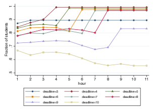
(a) Science and technology track

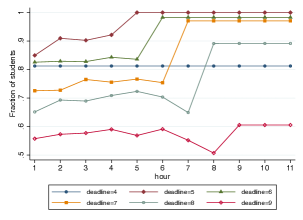
(b) Social science and humanities

Second, Table 3 reports descriptive evidence on time constraints. To begin with, 10,003 (47.4% of total) students from the science and technology track and 3,303 (54.2% of total) students from the social science and humanities track changed their choices in the final round. Among these students, 1,208 (5.7% of total) students from the science and technology track, and 577 (9.5% of total) students from the social science and humanities track, are nonetheless rejected despite their last-hour changes. These students are potentially harmed by the time constraints, as they could have been assigned if there had been additional time. If we look further into these students, 1,161 of the unassigned students from the science and technology track (5.5%) had a score higher than or equal to the final cutoff of a university to which they applied in previous hours. This figure is 325 for unassigned students from the social science and humanities track (5.3%). These students have indicated an acceptable choice at some point during their application. However, they were not assigned when the application ended. This might indicate the existence of justified envy, where some students prefer a university to be unassigned and have a score higher than the cutoff of that preferred university. It is worth mentioning that, students could apply in the ending round to a safe choice, where their scores are way above the cutoff, increasing their chance of assignment. Therefore, focusing on the final assignments, we might underestimate the magnitude of justified envy.

Table 3: Application behavior and assignment outcome

	Science and technology	Social science and humanities
$\#$ changed at final round	10,003	3,303
$\#$ changed at final round and are rejected	1,208	577
$\#$ unassigned but with a score $\geq$ final cutoff of a university applied previously	1,161	325

The staggered closing rule used by the IM procedure could put some students (those ranked higher in a batch) in a better position than others (those ranked bottom in a batch) regarding the information they receive. We do not observe a significant impact of information advantage or disadvantage around the cutoff. Indeed, additional factors could affect the cross-batch comparisons, such as how many students there are and how correlated preferences are within each batch. The fact that IM provides students with the same information can also backfire the information utilization. Students with higher scores do not need much information, while students with lower scores may not have enough information to help their application, given the imposed deadline.

6 Conclusions

With the advance in information technology, more school choice and college admission systems have started to adopt dynamic mechanisms, allowing students to interact and receive feedback during the application, unlike the traditional environment of static applications. This paper points out that time constraints might undermine these improvements.

In the context of college admissions, we first analyze theoretically the effects of time constraint on assignment outcomes, and we compare it with the standard DA mechanism. From an ex-post perspective it is not possible to rank these mechanisms. However, we prove that if a student receives a preferred outcome under TCDM, there is another student with higher priority who is not assigned under TCDM while he is assigned under DA. From an ex-ante perspective, we show that TCDM gives students a (weakly) higher probability of being assigned to their first choice and of remaining unassigned, but a lower probability of being assigned to the other options. We then illustrate our results in the real-life case of the dynamic mechanism used in the province of Inner Mongolian in China. We describe how students behave in data and provide evidence of the effects of time constraints on the final assignments. In particular, we show that the procedure’s outcome may not be stable due to time constraints.

Our paper opens the door for future studies. One challenge in utilizing field data generated by the dynamic mechanism is that we do not observe the students’ actual preferences. Lab experiments can address this issue by controlling for students’ preferences. Therefore, future research may think of running experiments to quantify the trade-offs of time constraints in dynamic environments more precisely. Furthermore, while it is crucial for students to have enough time to revise their options, one may wonder how the design of information could speed up the lengthy revision process. In the case of the IM procedure, every student receives the same type of information, whereas some need more information than others. Improving information design under such dynamic mechanisms could potentially alleviate the time constraints.

Appendix

Appendix A The extensive-form game induced by TCDM.

We describe the game induced by TCDM in this section. Most of the definitions are based on Klijn, Pais, and Vorsatz (2019). The game has the following elements.

• A finite set of players $I$, which corresponds to the set of students.

• A set of actions $A_{i}=C\cup\{i\}$ for each student $i$. This set includes all possible applications that a student might potentially make at each point of the the game, including the “no college” option $\{i\}$. Let $A\equiv\cup_{i\in I}A_{i}$.

  We make the following convention. If in a given round a student does not change her application, we let her apply to the same college.

• A set of nodes or histories $H$, where

  • the initial node or empty history $h_{0}$ is an element of $H$,

  • each $h\in H\setminus\{h_{0}\}$ takes the form $h=(a_{1},a_{2},\ldots,,a_{k})$ for some finitely many actions $a_{i}\in A$, and

  • if $h=(a_{1},a_{2},\ldots,,a_{k})\in H\setminus\{h_{0}\}$ for some $k>1$, then $(a_{1},a_{2},\ldots,,a_{k-1})\in H\setminus\{h_{0}\}$.

  A history is a sequence of application, one for each student, but each student may have applied more than once. For example, a history $(a_{1},a_{2},\ldots,,a_{k})$ means that student $1$ have applied to college $a_{1}$ in the first round, student $2$ to college $a_{2}$ in the first round, and so on for the first $|I|$ elements. The element $|I|+1$ is the application of student $1$ in the second round, element $|I|+2$ is the application of student $2$ in the second round, and so on, and so forth for the rest of the elements.

  The set of actions available to a student $i$ whose turn it is to move after history $h\in H$, is $C\cup\{i\}$.

• A set of end histories $E\equiv\{h\in H:(h,a)\notin H\text{ for all }a\in A\}$. In particular, the set of end node is the set of all histories of length $T\cdot|I|$.

• A function $\iota:H\setminus E\rightarrow I$ that indicates whose turn it is to move at each decision node in $H\setminus E$.

  We assume, without loss of generality, that students move sequentially at each round. Student $1$ moves first, $2$ moves second, and so on. Thus, for every non-terminal history $h$, the player function is

  $$\iota(h)=i_{|h|(\bmod N)+1},$$

  where $|h|$ is the length of the sequence $h$.

• An information set $\mathcal{I}_{i}$, which is a partition of the set $\{h:\iota(h)=i\}$, where $h,h^{\prime}\in I_{i}\in\mathcal{I}_{i}$ if the first $|h|-(i-1)$ elements of the two histories are the same. That is, when a student applies in a given round, she does not know the colleges to which other students applied in the same round, but she knows to which they applied in the previous rounds.

• An outcome function $g:E\rightarrow\mathcal{M}$ that associates each terminal history with a matching, where $\mathcal{M}$ is the set of all matchings.

For any history $h$ reached at the end of a round, that is, $|h|=k|I|$ for some $k=1,\ldots,T-1$, let $\mu^{h}$ be the matching found by considering the applications of students as defined by the last $N$ elements of the sequence. Said differently, it is the matching found by the last applications, where student $i_{n}$ applies to college $c_{N(k-1)+n}$. Thus, $\mu^{h}$ is the tentative matching at history $h$.

For any two terminal histories $h,h^{\prime}$, a student prefers $h$ over $h^{\prime}$ if and only if $\mu^{h}(i)P_{i}\mu^{h^{\prime}}(i)$, where $\mu^{h}(i)\in C\cup\{i\}$ is the assignment of student $i$ at $\mu^{h}$.

Definition 3.

A (pure) strategy for student $i$ in this extensive–form game is a function $\sigma_{i}:\mathcal{I}_{i}\rightarrow A$, such that $\sigma({I}_{i})\in C\cup\{i\}$, for all ${I}_{i}\in\mathcal{I}_{i}$.

Given a matching $\mu$ and a college $c$, a cutoff $f^{\mu}_{c}\in\mathbb{R}$ is the minimum score among all the admitted students if the colleges reaches its capacity, and $0$ if there is remaining capacity.

Definition 4.

(Straightforward strategies) A student $i$, with priority $s_{i}$ (that is, with a score in the exam equals to $s_{i}$) is said to follow straightforward strategy if at every history $h$ such that $\iota(h)=i$, her strategy $\sigma_{i}(h)$ is such that

$$\sigma_{i}(h)\coloneqq\max_{\succ_{i}}\;\{c\in C\cup\{i\}:s_{i}\geq f^{\mu}_{c}\},$$ (1)

where $\mu$ is the matching induced by $h$, $\mu^{h}$.

That is, at every history after which the student has to move, she applies to the most preferred college among those would accept her. It may be that she chooses the college where she is tentative assigned at that round.

Appendix B Proofs of Section 3.

Proof of Proposition 1.

Proof.

When students follow straightforward strategies, the process of applications is equivalent to the DA algorithm. Thus, TCDM stops when it reaches the stable matching. Next, suppose that the mechanism stops at an unstable matching. Then, there is a student $i$ who prefers a college $c$ to her current assignment, and has a score higher than that college’s cutoff. As students only apply to colleges after being rejected, this means that the student did not apply to $c$ and then she skipped $c$ in a previous step. But this contradicts the assumption that students follow straightforward strategies. ∎

Proof of Proposition 2.

Proof.

Let $\mu$ denote the matching resulting when all students play straightforward strategies. From Proposition 1, we know that $\mu$ is the unique stable matching and is efficient. Suppose now there is another matching $\mu^{\prime}$, which is obtained when all students but $i$ play straightforward strategies, and $i$ plays a deviating strategy. $i$ prefers the college $c$ that he is assigned to at $\mu^{\prime}$ than the one he receives at $\mu$. Then, there must be a student $j$ who has higher priority than $i$ who is assigned to $c$ at $\mu$ (otherwise $\mu$ is not stable). Clearly, student $j$ does not apply to $c$ in the process where $\mu^{\prime}$ is reached, so he is assigned to a preferred college $c^{\prime}$. This implies that there is a student $l$ who is assigned to $c^{\prime}$ at $\mu$ but not at $\mu^{\prime}$. Again, it must be the case that $l$ does not apply $c^{\prime}$ when the matching $\mu^{\prime}$ is reached. Continuing with this reasoning, as the number of student is finite, we will eventually reach student $i$. Then we construct an exchange cycle where, departing from $\mu$ all students students in the cycle are made better off, this contradicts to the fact that $\mu$ is efficient. Therefore, student $i$ can not do better than following straightforward strategy, and a profile where students follow strategies is indeed an equilibrium in absence of time constraint. ∎

Appendix C Ex-ante comparisons with correlated preferences

We consider 4 students to be assigned to 4 colleges, each with only one seat. As before, students priorities are such that student $i_{1}$ has the highest priority, followed by $i_{2}$, $i_{3}$ and $i_{4}$. Student’s ordinal preference is derived from the utility that takes the following form:

$$u_{c}(i)=\delta v_{c}+(1-\delta)\epsilon_{ic}.$$

The utility of individual $i$ for attending college $c$ consists two parts. The first part is a common utility component, denoted by $v_{c}$, and the second part is an idiosyncratic utility component that is unique to a student-college pair, denoted by $\epsilon_{ic}$. Both $v_{c}$ and $\epsilon_{ic}$ are drawn independently and identically on $[0,1]$ according to uniform distribution. The parameter $\delta$ measures the correlation of preferences, when $\delta=0$, we are back to the uniform and i.i.d preferences studied in Example 3, and when $\delta=1$, students’ preferences are identical. Students follow straightforward strategies under TCDM where $T=2$, and truth-telling strategies under DA.

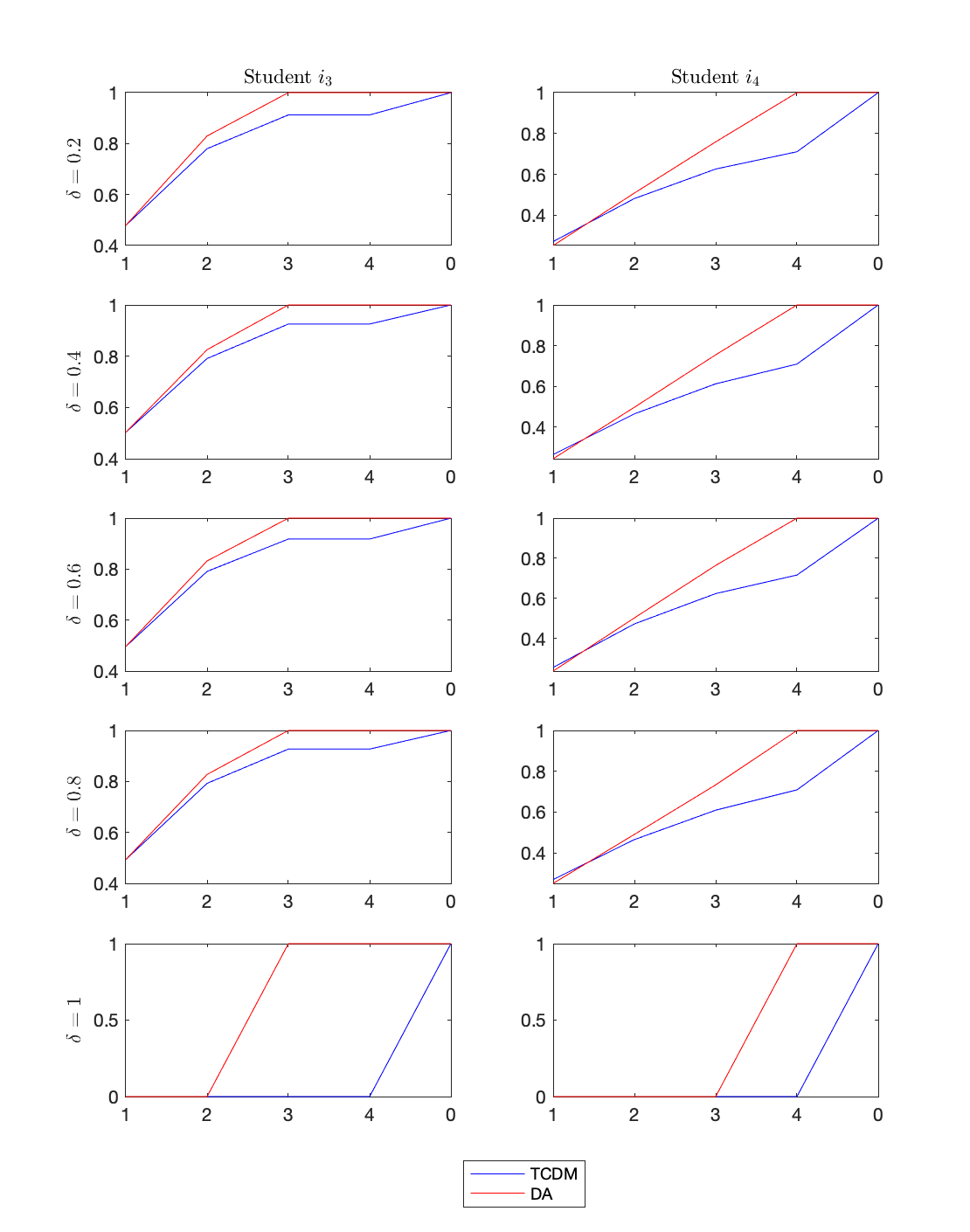
Figure C.1: CDF of assignment probabilities for students who are constrained with time

Notes: We ran 2000 simulations and take the average probabilities. Each row takes a different correlation parameter, and we look at the correlation parameter from $0.2$ to $1$ by a grid of $0.2$. Each column indicates a different student. In each subplot, x-axis indicates the CDF of being assigned to the first choice, the second choice, the third choice, the fourth choice and being unassigned.

Figure C.1 presents the simulated probabilities under both TCDM and DA for the two time-constrained students, namely $i_{3}$ and $i_{4}$. The results suggest patterns similar to what was shown in Example 3. When preferences are correlated but not identical ($\delta\neq 1$), then for $i_{3}$, DA yields a higher or equal probability to TCDM for being assigned to the first to the fourth choice. Similarly, for student $i_{4}$, except for the first choice, DA also yields a higher probability of being assigned to the second to the fourth choice. When preferences are identical, both of them are unassigned under TCDM; in this case, they are the most constrained with time.

Appendix D Additional information on empirical results

D.1 Descriptive statistics

Table D.1: Summary statistics from application data of final hour in 2018

	Science and technology track	Social science and humanities track
	(1)	(2)
Panel A: Student characteristics
Female	0.49	0.79
Ethnicity
- non-Han	0.24	0.25
Exam score (incl. bonus)	547.66	542.35
	(48.60)	(29.86)
Exam score (excl. bonus)	545.54	540.21
	(48.62)	(29.78)
Fraction of students ina
- Batch 1 ($\geq 670$)	0.01
- Batch 2 ($640-669$)	0.04	0.003
- Batch 3 ($610-639$)	0.08	0.03
- Batch 4 ($580-609$)	0.13	0.10
- Batch 5 ($550-579$)	0.18	0.237
- Batch 6 ($520-549$)	0.21	0.36
- Batch 7 ($490-519$)	0.24	0.27
- Batch 8 ($460-489$)	0.11
Panel B: Admission outcomes
- Admitted to a university based on final choices according to rank up to quotab	0.89	0.83
- Admitted to a university based on final choices according to cutoff	0.89	0.84
Number of students	21,107	6,089
Panel C: Universities
Planned quota	67.97	23.64
	(209.28)	(84.15)
Final quota	69.85	24.41
	(219.14)	(88.39)
Number of universities	291	211

Notes: ^aThe score cutoffs to divide groups are indicated in brackets. In both tracks, there are no students who have score less than 460, the last batch according to the definition of the clearinghouse. In social science and humanities track, there are no students in Batch 1 nor Batch 8. ^bThe first measure is based on whether a students is among the top most preferred students up to the allowed quota in their last-hour choices. The second measure is based on whether a student has a cutoff higher than or equal to the final cutoff at their last-hour choices. The two measures lead to a difference of 4 students in the science and technology track, and 58 students in the social science and humanities track.

D.2 Data linking

In order to solve the issue of multiple observations having the same characteristics, we use the two rules below.

Rule 1. Program priority: in a given university, if there is one observation who has the same characteristics and program choices as another observation at a previous hour, then we consider these two observations are the same student, and this student has not changed program choice nor university choice.

Rule 2. University priority: in a given university, if there is one observation who has the same characteristics as another student at a previous hour, then we consider these two observations are the same student, in addition we consider this student has not changed university choice.

The first rule essentially considers two students at two different hours that have the same characteristics together with university and program choices the same student. After first linking students using program priority, we use the second rule to link those who might have changed their program choices but not their university choices. When we cannot find a match, we search for another student with the same characteristics in another university at an earlier hour. We implemented the following procedure in Java.

1. For students observed in the last hour $T$, assign each of them an ID.

   1. At $T-1$, for those who are inactive in both hours, assign them the IDs from $T$.

   2. For those who are active in one of these two hours, for each university $j$, consider all students applied to it:

      1. If there exist some students with the same four characteristics that are in university $j$ at $T-1$ as well as in university $j$ at $T$, and have the same choices for programs, then, by Rule 1, these students are matched, and are assigned with IDs from those at $T$.

      2. Among the rest of students, if there are some students with the same four characteristics that are in university $j$ at $T-1$ as well as in university $j$ at $T$, then by Rule 2, these students are matched and are assigned with IDs from those at $T$.

      3. Among the rest of unmatched students, i.e. those who applied to $j$ at $T$ but not at $T-1$,

         1. If there are students, in other universities excluding $j$, that have the same four characteristics as those from $T$, then assign these students the IDs of students from $T$, following the order in the original data.

         2. If there are students still unmatched, assign them new IDs.

2. Repeat the procedure for $T-k$ until the hour 1, which gives us the student-level application data over time.

References

- (1)
- Abdulkadiroğlu and Sönmez (2003) Abdulkadiroğlu, A., and T. Sönmez (2003): “School choice: A mechanism design approach,” The American Economic Review, 93(3), 729–747.
- Azevedo and Leshno (2016) Azevedo, E. M., and J. D. Leshno (2016): “A supply and demand framework for two-sided matching markets,” Journal of Political Economy, 124(5), 1235–1268.
- Balinski and Sönmez (1999) Balinski, M., and T. Sönmez (1999): “A tale of two mechanisms: student placement,” Journal of Economic theory, 84(1), 73–94.
- Bó and Hakimov (2020) Bó, I., and R. Hakimov (2020): “Iterative versus standard deferred acceptance: Experimental evidence,” The Economic Journal, 130(626), 356–392.
- Bó and Hakimov (2022) (2022): “The Iterative Deferred Acceptance Mechanism,” Games and Economic Behavior, forthcoming.
- Calsamiglia, Fu, and Güell (2020) Calsamiglia, C., C. Fu, and M. Güell (2020): “Structural estimation of a model of school choices: The boston mechanism versus its alternatives,” Journal of Political Economy, 128(2), 642–680.
- Chen and Pereyra (2019) Chen, L., and J. S. Pereyra (2019): “Self-selection in school choice,” Games and Economic Behavior, 117, 59–81.
- Chen and Kesten (2017) Chen, Y., and O. Kesten (2017): “Chinese college admissions and school choice reforms: A theoretical analysis,” Journal of Political Economy, 125(1), 99–139.
- Ding and Schotter (2017) Ding, T., and A. Schotter (2017): “Matching and chatting: An experimental study of the impact of network communication on school-matching mechanisms,” Games and Economic Behavior, 103, 94–115.
- Dubins and Freedman (1981) Dubins, L. E., and D. A. Freedman (1981): “Machiavelli and the Gale-Shapley algorithm,” The American Mathematical Monthly, 88(7), 485–494.
- Dur, Hammond, and Kesten (2021) Dur, U., R. G. Hammond, and O. Kesten (2021): “Sequential school choice: Theory and evidence from the field and lab,” Journal of Economic Theory, 198, 105344.
- Dur, Hammond, and Morrill (2017) Dur, U., R. G. Hammond, and T. Morrill (2017): “Identifying the harm of manipulable school-choice mechanisms,” American Economic Journal: Economic Policy.
- Gale and Shapley (1962) Gale, D., and L. S. Shapley (1962): “College Admissions and the Stability of Marriage,” The American Mathematical Monthly, 69(1), 9–15.
- Gong and Liang (2020) Gong, B., and Y. Liang (2020): “A Dynamic Matching Mechanism for College Admissions: Theory and experiments,” Working paper.
- Grenet, He, and Kübler (2022) Grenet, J., Y. He, and D. Kübler (2022): “Preference Discovery in University Admissions: The Case for Dynamic Multioffer Mechanisms,” Journal of Political Economy, 130(6), 000–000.
- Hassidim, Marciano, Romm, and Shorrer (2017) Hassidim, A., D. Marciano, A. Romm, and R. I. Shorrer (2017): “The mechanism is truthful, why aren’t you?,” American Economic Review, 107(5), 220–24.
- He (2012) He, Y. (2012): “Gaming the boston school choice mechanism in beijing,” Manuscript, Toulouse School of Economics.
- Klijn, Pais, and Vorsatz (2019) Klijn, F., J. Pais, and M. Vorsatz (2019): “Static versus dynamic deferred acceptance in school choice: Theory and experiment,” Games and Economic Behavior, 113, 147–163.
- Luflade (2018) Luflade, M. (2018): “The value of information in centralized school choice systems,” Duke University, 4(6), 7.
- Pais and Pintér (2008) Pais, J., and Á. Pintér (2008): “School choice and information: An experimental study on matching mechanisms,” Games and Economic Behavior, 64(1), 303–328.
- Pathak (2017) Pathak, P. A. (2017): “What really matters in designing school choice mechanisms,” Advances in Economics and Econometrics, 1, 176–214.
- Pathak and Shi (2021) Pathak, P. A., and P. Shi (2021): “How well do structural demand models work? Counterfactual predictions in school choice,” Journal of Econometrics, 222(1), 161–195.
- Rees-Jones (2018) Rees-Jones, A. (2018): “Suboptimal behavior in strategy-proof mechanisms: Evidence from the residency match,” Games and Economic Behavior, 108, 317–330.
- Roth (1982) Roth, A. E. (1982): “The economics of matching: Stability and incentives,” Mathematics of operations research, 7(4), 617–628.
- Shorrer and Sóvágó (2021) Shorrer, R., and S. Sóvágó (2021): “Dominated choices in a strategically simple college admissions environment: The effect of admission selectivity,” Discussion paper, Working paper.
- Stephenson (2016) Stephenson, D. G. (2016): “Continuous feedback in school choice mechanisms,” Working paper.