Production rates of $D_{s}^{+}D_{s}^{-}$ and $D\bar{D}$ molecules in $B$ decays

Abstract

Motivated by the recently discovery of a charmonium $X(3960)$ in $B$ decays by the LHCb Collaboration, the likely existence of two bound/virtual states (denoted by $X_{s\bar{s}}$ and $X_{q\bar{q}}$) below the $D_{s}^{+}D_{s}^{-}$ and $\bar{D}D$ mass thresholds has been re-examined recently. In this work, we employ the effective Lagrangian approach to calculate their production rates in $B$ decays utilizing triangle diagrams. Our results show that the production yields of $B^{+}\to X_{s\bar{s}}K^{+}$ and $B^{+}\to X_{q\bar{q}}K^{+}$ are of the order of $10^{-4}$, in agreement with the relevant experimental data, which indicates that, if the $D_{s}^{+}D_{s}^{-}$ and $\bar{D}D$ bound states indeed exist, they can be detected in $B$ decays. Moreover, we calculate the production rate of $B^{+}\to X(3960)K^{+}$ assuming that $X(3960)$ is a resonant state of $D_{s}^{+}D_{s}^{-}$ and find that it is also of the order of $10^{-4}$ but a bit smaller than that as a $D_{s}^{+}D_{s}^{-}$ bound state.

I Introduction

In 2004, the Belle Collaboration observed a state around 3940 MeV in the $J/\psi\omega$ invariant mass distribution of the $B\to J/\psi\omega K$ decay Abe et al. (2005), which was later confirmed by the BaBar Collaboration in the same process but the mass was determined to be 3915 MeV Aubert et al. (2008). In 2009, the Belle Collaboration observed a state near 3915 MeV in the $\gamma\gamma\to J/\psi\omega$ reaction Uehara et al. (2010). Later the BaBar Collaboration determined the quantum number of this state to be $J^{PC}=0^{++}$ Lees et al. (2012). In 2020, the LHCb Collaboration observed a similar state $\chi_{c0}(3930)$ in the $D^{+}D^{-}$ mass distribution of the $B^{+}\to D^{+}D^{-}K^{+}$ decay Aaij et al. (2020a, b). In the Review of Particle Physics (RPG) Zyla et al. (2020), all these states are referred to as $\chi_{c0}(3915)$ and viewed as a candidate for the $\chi_{c0}(2P)$ charmonium Duan et al. (2020, 2021). Very recently, the LHCb Collaboration reported a charmonium state named as $X(3960)$ with $J^{PC}=0^{++}$ in the $D_{s}^{+}D_{s}^{-}$ mass distribution of the $B^{+}\to D_{s}^{+}D_{s}^{-}K^{+}$ decay. Its mass and width are determined to be $m=3955\pm 6\pm 11$ MeV and $\Gamma=48\pm 17\pm 10$ MeV LHC (2022a, b).

Given that the mass of $X(3960)$ is very different from that of $\chi_{c0}(3915)$, they are not likely to be the same state. It is also difficult to interpret $X(3960)$ as a conventional charmonium because the mass of $\chi_{c0}(3P)$ (in the quark model) is around 4200 MeV  Barnes et al. (2005); Li and Chao (2009). In Ref. Bayar et al. (2022), M. Bayar et al. argued that in the chiral unitary approach there exist two states below the $D\bar{D}$ and $D_{s}^{+}D_{s}^{-}$ thresholds, respectively, and the new $X(3960)$ can be understood as an enhancement in the $D_{s}^{+}D_{s}^{-}$ mass distribution. In Ref. Xin et al. (2022), Xin et al. interpreted $X(3960)$ as a $J^{PC}=0^{++}$ $D_{s}^{+}D_{s}^{-}$ molecule in the QCD sum rules approach. With a leading order contact range effective field theory Ji et al. showed that either a bound state or a virtual state below the $D_{s}^{+}D_{s}^{-}$ mass threshold is needed to describe the $D_{s}^{+}D_{s}^{-}$ mass distribution of the $B^{+}\to D_{s}^{+}D_{s}^{-}K^{+}$ decay Ji et al. (2022).

The likely existence of molecules near the $D\bar{D}$ and $D_{s}^{+}D_{s}^{-}$ mass thresholds has been studied in several approaches before the experimental discoveries. In Ref. Prelovsek et al. (2021), Prelovsek et al. performed lattice QCD simulations of coupled-channel $D\bar{D}$ and $D_{s}^{+}D_{s}^{-}$ interactions and found the existence of two bound states near the $D\bar{D}$ and $D_{s}^{+}D_{s}^{-}$ mass thresholds. In Ref. Gamermann et al. (2007), Gamermann et al. obtained a $I(J^{PC})=0(0^{++})$ narrow resonance with a mass of 3719 MeV, which mainly couples to the $D\bar{D}$ and $D_{s}\bar{D}_{s}$ channels. In our previous works Liu et al. (2019); Wu et al. (2021), we investigated the $D\bar{D}$ interaction in the one boson exchange (OBE) model and found that a large cutoff of $\Lambda=1.415$ GeV is needed to generate a $D\bar{D}$ bound state. On the other hand, in order to reproduce $X(3872)$ as a $D^{\ast}\bar{D}$ bound state in the OBE model, one only needs a cutoff of $\Lambda=1.01$ GeV. From this, one concludes that the $D\bar{D}$ interaction is less attractive than the $D^{\ast}\bar{D}$ interaction, in agreement with several recent studies Liu and Geng (2021); Dong et al. (2021); Peng et al. (2022).

In Refs. Wang et al. (2021a); Deineka et al. (2022), the authors described the $D\bar{D}$ mass distribution of $\gamma\gamma\to D\bar{D}$ and demonstrated the existence of a bound state near the $D\bar{D}$ mass threshold. In Ref. Dai et al. (2016), considering the state $X(3720)$ mainly coupled to $D\bar{D}$, Dai et al. predicted the $D\bar{D}$ mass distribution of the $B^{-}\to D^{0}\bar{D}^{0}K^{-}$ process. In Ref. Li and Voloshin (2015), assuming $\chi_{c0}(3915)$ as a $D_{s}^{+}D_{s}^{-}$ bound state, Li et al. estimated the branching ratio of the $B^{+}\to\chi_{c0}(3915)K^{+}$ decay to be $6\times 10^{-4}$. In this work, we assume that there exist two molecules near the $D\bar{D}$ and $D_{s}^{+}D_{s}^{-}$ mass thresholds, denoted as $X_{q\bar{q}}$ and $X_{s\bar{s}}$, and employ the effective Lagrangian approach to investigate their production rates in $B$ decays via the triangle mechanism. Such an approach has been applied to study the production of $P_{c}$ and $P_{cs}$ in the $\Lambda_{b}\to J/\psi pK$ Wu and Chen (2019) and $\Xi_{b}\to J/\psi\Lambda K$ decays Lu et al. (2021). The production rates of $D\bar{D}$ and $D_{s}^{+}D_{s}^{-}$ molecules in $B$ decays are helpful to probe the nature of $X(3960)$ as well as to understand the $D\bar{D}$ and $D_{s}^{+}D_{s}^{-}$ interactions.

This work is organized as follows. We introduce the triangle mechanism for the decays of $B^{+}\to X_{s\bar{s}}K^{+}$ and $B^{+}\to X_{q\bar{q}}K^{+}$ and the effective Lagrangian approach in Sec. II. Results and discussions are given in Sec. III, followed by a short summary in the last section.

II Theoretical formalism

\begin{overpic}[scale={.22}]{Wemission.png} \end{overpic}

Figure 1: External $W$-emission for $B^{+}\to D_{s}^{+}\bar{D}^{*0}$ and $B^{+}\to D_{s}^{\ast+}\bar{D}^{0}$.

The $B$ decays are a good platform to study the weak interaction and exotic states Cheng et al. (2005); Cheng and Yang (2008); Chen (2022); Wang et al. (2021b). In this work, we employ the triangle diagram to investigate the weak decays of $B^{+}\to X_{q\bar{q}}K^{+}$ and $B^{+}\to X_{s\bar{s}}K^{+}$. At the quark level, the decays of $B^{+}\to D_{s}^{+}\bar{D}^{*0}$ and $B^{+}\to D_{s}^{\ast+}\bar{D}^{0}$ can both proceed through the external $W$-emission mechanism shown in Fig. 1. Referring to the Review of Particle Physics Zyla et al. (2020), the absolute branching fractions of the decay modes $B^{+}\to D_{s}^{+}\bar{D}^{\ast 0}$ and $B^{+}\to D_{s}^{\ast+}\bar{D}^{0}$ are $(8.2\pm 1.7)\times 10^{-3}$ and $(7.6\pm 1.6)\times 10^{-3}$, respectively, which are larger than those of the $B$ meson decaying into a charmonium and a $K^{+}$. Then, taking into account the interaction vertices of $\bar{D}^{\ast 0}\to{D}_{s}^{-}K^{+}$ and $D_{s}^{\ast+}\to D^{0}K^{+}$, the $D_{s}^{+}D_{s}^{-}$ and $\bar{D}^{0}D^{0}$ molecules can be dynamically generated. We illustrate the decays of $B^{+}\to X_{s\bar{s}}K^{+}$ and $B^{+}\to X_{q\bar{q}}K^{+}$ at the hadron level via the triangle diagrams shown in Fig. 2. In the following, we introduce the effective Lagrangians relevant to the computation of the Feynman diagrams shown in Fig. 2.

\begin{overpic}[scale={.24}]{triangle.png} \end{overpic}

Figure 2: Triangle diagrams accounting for the two B decays: (a) $B^{+}\to D_{s}^{+}\bar{D}^{*0}\to X_{s\bar{s}}K^{+}$ and (b) $B^{+}\to D_{s}^{\ast+}\bar{D}^{0}\to X_{q\bar{q}}K^{+}$.

The effective Hamiltonian describing the weak decays of $B^{+}\to D_{s}^{+}\bar{D}^{\ast 0}$ and $B^{+}\to D_{s}^{\ast+}\bar{D}^{0}$ has the following form

$$\mathcal{H}_{eff}=\frac{G_{F}}{\sqrt{2}}V_{cb}V_{cs}[c_{1}^{eff}\mathcal{O}_{1}+c_{2}^{eff}\mathcal{O}_{2}]+h.c.,$$ (1)

where $G_{F}$ is the Fermi constant, $V_{bc}$ and $V_{cs}$ are the Cabibbo-Kobayashi-Maskawa (CKM) matrix elements, $c_{1,2}^{eff}$ are the effective Wilson coefficients, and $\mathcal{O}_{1}$ and $\mathcal{O}_{2}$ are the four-fermion operators of $(s\bar{c})_{V-A}(c\bar{b})_{V-A}$ and $(\bar{c}c)_{V-A}(s\bar{b})_{V-A}$ with $(\bar{q}q)_{V-A}$ standing for $\bar{q}\gamma_{\mu}(1-\gamma_{5})q$ Buras (1998); Geng et al. (2018); Han et al. (2021).

The amplitudes of $B^{+}\to D_{s}^{+}\bar{D}^{\ast 0}$ and $B^{+}\to D_{s}^{\ast+}\bar{D}^{0}$ can be written as the products of two hadronic matrix elements Ali et al. (1998); Qin et al. (2014)

$$\mathcal{A}\left(B^{+}\to D_{s}^{+}\bar{D}^{\ast 0}\right) = \frac{G_{F}}{\sqrt{2}}V_{cb}V_{cs}a_{1}\left\langle D_{s}^{+}|(s\bar{c})|0\right\rangle\left\langle\bar{D}^{\ast 0}|(c\bar{b})|B^{+}\right\rangle$$ (2)

$$\mathcal{A}\left(B^{+}\to D_{s}^{\ast+}\bar{D}^{0}\right) = \frac{G_{F}}{\sqrt{2}}V_{cb}V_{cs}a_{1}^{\prime}\left\langle D_{s}^{\ast+}|(s\bar{c})|0\right\rangle\left\langle\bar{D}^{0}|(c\bar{b})|B^{+}\right\rangle$$ (3)

where $a_{1}^{(\prime)}=c_{1}^{eff}+c_{2}^{eff}/N_{c}$ with $N_{c}=3$ the number of colors. It should be noted that $a_{1}$ and $a_{1}^{\prime}$ can be obtained in the factorization approach Bauer et al. (1987).

The current matrix elements between a pseudoscalar meson or vector meson and the vacuum have the following form:

$$\left\langle D_{s}^{+}|(s\bar{c})|0\right\rangle=g_{\mu\nu}f_{D_{s}^{+}}p^{\nu}_{D_{s}^{+}},~{}~{}\left\langle D_{s}^{\ast+}|(s\bar{c})|0\right\rangle=m_{D_{s}^{\ast+}}f_{D_{s}^{\ast+}}\epsilon_{\mu}^{*},$$ (4)

where $f_{D_{s}}$ and $f_{D_{s}^{\ast+}}$ are the decay constants for $D_{s}$ and $D_{s}^{\ast+}$, respectively, and $\epsilon_{\mu}^{*}$ is the polarization vector of $D_{s}^{\ast+}$.

The hadronic matrix elements can be parameterised in terms of a few form factors Verma (2012)

$$\left\langle\bar{D}^{\ast 0}|(c\bar{b})|B^{+}\right\rangle=\epsilon_{\alpha}^{*}\left\{-g^{\mu\alpha}(m_{\bar{D}^{\ast 0}}+m_{B^{+}})A_{1}\left(q^{2}\right)+P^{\mu}P^{\alpha}\frac{A_{2}\left(q^{2}\right)}{m_{\bar{D}^{\ast 0}}+m_{B^{+}}}\right.$$ (5)

$$+i\varepsilon^{\mu\alpha\beta\gamma}P_{\beta}q_{\gamma}\left.\frac{V\left(q^{2}\right)}{m_{\bar{D}^{\ast 0}}+m_{B^{+}}}+q^{\mu}P^{\alpha}\left[\frac{m_{\bar{D}^{\ast 0}}+m_{B^{+}}}{q^{2}}A_{1}\left(q^{2}\right)-\frac{m_{B^{+}}-m_{\bar{D}^{\ast 0}}}{q^{2}}A_{2}\left(q^{2}\right)-\frac{2m_{\bar{D}^{\ast 0}}}{q^{2}}A_{0}\left(q^{2}\right)\right]\right\},$$

$$\left\langle\bar{D}^{0}|(c\bar{b})|B^{+}\right\rangle=\left(p_{B^{+}}+p_{\bar{D}^{0}}\right)^{\mu}F_{1D}(q^{\prime 2})+q^{\prime\mu}F_{2D}(q^{\prime 2}),$$ (6)

where $q$ and $q^{\prime}$ represent the momentum of $D_{s}^{+}$ and ${D}_{s}^{\ast+}$, respectively, and $P=(p_{B^{+}}+p_{\bar{D}^{\ast 0}})$. The form factors of $F_{1,2D}(t)$, $A_{0}(t)$, $A_{1}(t)$, $A_{2}(t)$, and $V(t)$ with $t\equiv q^{(\prime)2}$ are parameterized as

$$X(t)=\frac{X(0)}{1-a\left(t/m_{B}^{2}\right)+b\left(t^{2}/m_{B}^{4}\right)},$$ (8)

which could well fit the transition form factors of $B\to\bar{D}^{(\ast)}$ as shown in Ref. Verma (2012).

The Lagrangian describing the interaction between the charmed mesons $D_{s}$, $D^{*}$ and a kaon has the following form

$$\mathcal{L}_{D_{s}D^{\ast}K} = -ig_{D_{s}D^{\ast}K}(D_{s}\partial^{\mu}KD^{\ast{\dagger}}_{\mu}-D_{\mu}^{*}\partial^{\mu}KD_{s}^{{\dagger}}),$$ (9)

where $g_{D_{s}D^{\ast}K}$ is the coupling constant.

Assuming that $X_{s\bar{s}}$ and $X_{q\bar{q}}$ are dynamically generated by the $D_{s}^{+}D_{s}^{-}$ and $\bar{D}D$ interactions, respectively, the relevant Lagrangians can be written as

$$\mathcal{L}_{X_{s\bar{s}}D_{s}^{+}D_{s}^{-}}(x) = g_{X_{s\bar{s}}D_{s}^{+}D_{s}^{-}}X_{s\bar{s}}(x)\int dy\Phi(y^{2})D_{s}^{+}(x+\frac{1}{2}y)D_{s}^{-}(x-\frac{1}{2}y),$$ (10)

$$\mathcal{L}_{X_{q\bar{q}}\bar{D}D}(x) = g_{X_{q\bar{q}}\bar{D}D}X_{q\bar{q}}(x)\int dy\Phi(y^{2})\bar{D}(x+\frac{1}{2}y)D(x-\frac{1}{2}y).$$ (11)

As $X_{s\bar{s}}$ and $X_{q\bar{q}}$ are bound states of $D_{s}^{+}D_{s}^{-}$ and $\bar{D}D$, we adopt the compositeness condition to estimate the couplings of $g_{X_{s\bar{s}}D_{s}^{+}D_{s}^{-}}$ and $g_{X_{q\bar{q}}\bar{D}D}$. The correlation function $\Phi(y^{2})$ is introduced to reflect the distribution of the two constituent hadrons in the molecule, which also renders the Feynman diagrams ultraviolet finite. Here we choose the Fourier transformation of the correlation function in form of a Gaussian function

$$\Phi(p^{2})\doteq\mbox{Exp}(-p_{E}^{2}/\Lambda^{2}),$$ (12)

where $\Lambda$ is a size parameter, which is expected to be around 1 GeV Ling et al. (2021a, 2022), and $p_{E}$ is the Euclidean momentum. The couplings, $g_{X_{s\bar{s}}D_{s}^{+}D_{s}^{-}}$ and $g_{X_{q\bar{q}}\bar{D}D}$, can be estimated by reproducing the binding energies of the $X_{s\bar{s}}$ and $X_{q\bar{q}}$ states via the compositeness condition Weinberg (1963); Salam (1962); Hayashi et al. (1967). The condition dictates that the coupling constant can be determined from the fact that the renormalization constant of the wave function of a composite particle should be zero. The compositeness condition can be estimated from the self energy

$$Z=1-\frac{d\Sigma(k_{0}^{2})}{d{k}_{0}^{2}}|_{{{k}_{0}=m_{X}}}=0.$$ (13)

With the above relevant Lagrangians, one can easily compute the corresponding amplitudes of Fig. 2,

$$\mathcal{A}_{a} =g_{X_{s\bar{s}}D_{s}^{+}D_{s}^{-}}\int\frac{d^{4}q_{3}}{(2\pi)^{4}}\frac{{\rm i}\mathcal{A}(B^{+}\to D_{s}^{+}\bar{D}^{\ast 0})\mathcal{A}\left(\bar{D}^{\ast 0}\to D_{s}^{-}K^{+}\right)}{\left(q_{1}^{2}-m_{\bar{D}^{\ast}}^{2}+im_{\bar{D}^{\ast}}\Gamma_{\bar{D}^{\ast}}\right)\left(q_{2}^{2}-m_{D_{s}^{+}}^{2}\right)\left(q_{3}^{2}-m_{D_{s}^{-}}^{2}\right)},$$ (14)

$$\mathcal{A}_{b} =g_{X_{q\bar{q}}\bar{D}^{0}D^{0}}\int\frac{d^{4}q_{3}}{(2\pi)^{4}}\frac{{\rm i}\mathcal{A}(B^{+}\to D_{s}^{\ast+}\bar{D}^{0})\mathcal{A}\left(D_{s}^{\ast+}\to D^{0}K^{+}\right)}{\left(q_{1}^{2}-m_{{D}_{s}^{\ast+}}^{2}+im_{{D}_{s}^{\ast+}}\Gamma_{{D}_{s}^{\ast+}}\right)\left(q_{2}^{2}-m_{\bar{D}^{0}}^{2}\right)\left(q_{3}^{2}-m_{D^{0}}^{2}\right)},$$ (15)

where $q_{1}$, $q_{2}$, and $q_{3}$ denote the momenta of $\bar{D}^{\ast 0}$, $D_{s}^{+}$, and $D_{s}^{-}$ for Fig. 2 (a) and $D_{s}^{\ast+}$, $\bar{D}^{0}$, and $D^{0}$ for Fig. 2 (b), and $p_{1}$ and $p_{2}$ represent the momenta of $K^{+}$ and $X_{s\bar{s}}(X_{q\bar{q}})$. The vertices of $X_{s\bar{s}}D_{s}^{+}D_{s}^{-}$ and $X_{q\bar{q}}\bar{D}^{0}D^{0}$ are parameterised as the couplings $g_{X_{s\bar{s}}D_{s}^{+}D_{s}^{-}}$ and $g_{X_{q\bar{q}}\bar{D}^{0}D^{0}}$, respectively. The $\bar{D}^{\ast 0}\to D_{s}^{-}K^{+}$ transition is expressed as $\mathcal{A}\left(\bar{D}^{\ast 0}\to D_{s}^{-}K^{+}\right)=g_{\bar{D}^{\ast 0}D_{s}^{-}K^{+}}p_{1}\cdot\varepsilon(q_{1})$, and the $D_{s}^{\ast+}\to D^{0}K^{+}$ transition is expressed as $\mathcal{A}(D_{s}^{\ast+}\to D^{0}K^{+})=g_{D_{s}^{\ast+}D^{0}K^{+}}p_{1}\cdot\varepsilon(q_{1})$. The weak decay amplitudes of $B^{+}\to D_{s}^{+}\bar{D}^{\ast 0}$ and $B^{+}\to D_{s}^{\ast+}\bar{D}^{0}$ are written as

$$\mathcal{A}(B\to D_{s}\bar{D}^{\ast}) =\frac{G_{F}}{\sqrt{2}}V_{cb}V_{cs}a_{1}f_{D_{s}}\{-q_{2}\cdot\varepsilon(q_{1})(m_{\bar{D}^{\ast 0}}+m_{B^{+}})A_{1}\left(q_{2}^{2}\right)$$ (16)

$$+(k_{0}+q_{1})\cdot\varepsilon(q_{1})q_{2}\cdot(k_{0}+q_{1})\frac{A_{2}\left(q_{2}^{2}\right)}{m_{\bar{D}^{\ast 0}}+m_{B^{+}}}+(k_{0}+q_{1})\cdot\varepsilon(q_{1})$$

$$[(m_{\bar{D}^{\ast 0}}+m_{B^{+}})A_{1}(q_{2}^{2})-(m_{B^{+}}-m_{\bar{D}^{\ast 0}})A_{2}(q_{2}^{2})-2m_{\bar{D}^{\ast 0}}A_{0}(q_{2}^{2})]\},$$

$$\mathcal{A}(B\to D_{s}^{\ast}\bar{D}) =\frac{G_{F}}{\sqrt{2}}V_{cb}V_{cs}a_{1}^{\prime}f_{D_{s}^{*}}m_{D_{s}^{*}}\varepsilon(q_{1})\cdot(k_{0}+q_{2})F_{1D}(q_{1}^{2}),$$

With the $B^{+}\to X_{s\bar{s}}(X_{q\bar{q}})K^{+}$ amplitudes determined above, the corresponding partial decay widths can be finally written as

$$\Gamma=\frac{1}{2J+1}\frac{1}{8\pi}\frac{|\vec{p}|}{m_{B}^{2}}\bar{|\mathcal{M}|}^{2},$$ (17)

where $J$ is the total angular momentum of the initial $B$ meson, the overline indicates the sum over the polarization vectors of final states, and $|\vec{p}|$ is the momentum of either final state in the rest frame of the $B$ meson.

III Results and Discussions

Table 1: Masses and quantum numbers of mesons relevant to the present work Zyla et al. (2020).

Meson	$I(J^{P})$	M (MeV)	Meson	$I(J^{P})$	M (MeV)
$B^{+}$	$\frac{1}{2}(0^{-})$	$5279.34$	$K^{+}$	$\frac{1}{2}(0^{-})$	$493.677$
$D^{0}$	$\frac{1}{2}(0^{-})$	$1864.84$	$D^{+}$	$\frac{1}{2}(0^{-})$	$1869.66$
$D^{\ast 0}$	$\frac{1}{2}(1^{-})$	$2006.85$	$D^{\ast+}$	$\frac{1}{2}(1^{-})$	$2010.26$
$D_{s}^{+}$	$0(0^{-})$	$1968.34$	$D_{s}^{*+}$	$0(1^{-})$	$2112.2$

The amplitudes of $B^{+}\to D_{s}^{+}\bar{D}^{0\ast}$ and $B^{+}\to D_{s}^{\ast+}\bar{D}^{0}$ are obtained by the naive factorization approach as shown in Eq. (13). In this work, we take $G_{F}=1.166\times 10^{-5}~{}{\rm GeV}^{-2}$, $V_{cb}=0.041$, $V_{cs}=0.987$, $f_{D_{s}}=250$ MeV, and $f_{D_{s}^{*}}=272$ MeV as in Refs. Zyla et al. (2020); Verma (2012); Aoki et al. (2020); Donald et al. (2012); Li et al. (2017). For the form factors, we adopt those of the covariant light-front quark model, e.g., $(F_{1D}(0),a,b)^{B^{+}\to\bar{D}^{0}}=(0.67,1.22,0.36)$, $(A_{0}(0),a,b)^{B\to\bar{D}^{\ast 0}}=(0.68,1.21,0.36)$, $(A_{1}(0),a,b)^{B\to\bar{D}^{\ast 0}}=(0.65,0.60,0.00)$, and $(A_{2}(0),a,b)^{B\to\bar{D}^{\ast 0}}=(0.61,1.12,0.31)$ Verma (2012). Note that the terms containing $V(q^{2})$ and $F_{2D}(q^{\prime 2})$ do not contribute to the processes we study here. We tabulate the masses and quantum numbers of relevant particles in Table 1. In terms of the branching ratios of $B^{+}\to D_{s}^{+}\bar{D}^{\ast 0}$ and $B^{+}\to D_{s}^{\ast+}\bar{D}^{0}$ we determine $a_{1}=0.93$ and $a_{1}^{\prime}=0.81$, consistent with the estimates of Ref. Ali et al. (1998). The couplings of $g_{D_{s}^{+}\bar{D}^{\ast 0}K^{+}}$ and $g_{D_{s}^{\ast+}\bar{D}^{0}K^{+}}$ are determined by the SU(3)-flavor symmetry, e.g., $g_{D_{s}^{+}\bar{D}^{\ast 0}K^{+}}=g_{D_{s}^{\ast+}\bar{D}^{0}K^{+}}=\sqrt{2}g_{\bar{D}^{\ast 0}\bar{D}^{0}\pi^{0}}$, where $g_{\bar{D}^{\ast 0}\bar{D}^{0}\pi^{0}}=11.7$ is obtained from the decay width of $D^{*0}\to D^{0}\pi^{0}$ Zyla et al. (2020). The couplings of $g_{X_{s\bar{s}}D_{s}^{+}D_{s}^{-}}$ and $g_{X_{q\bar{q}}\bar{D}^{0}D^{0}}$ depend on whether the $X_{s\bar{s}}$ and $X_{q\bar{q}}$ states are below or above the mass thresholds of $D_{s}^{+}D_{s}^{-}$ and $\bar{D}D$, which will be specified below.

It is necessary to analyse the uncertainties of our results, which mainly come from the coupling constants needed to evaluate the triangle diagrams. In the weak interaction vertex, the uncertainties for the parameters $X(0)$, $a$ and $b$ of the transition form factors estimated in Ref. Verma (2012) are quite small and can be neglected. On the other hand, the uncertainties in the experimental branching ratios of $B\to\bar{D}^{0}D_{s}^{\ast+}/\bar{D}^{\ast 0}D_{s}^{+}$ can propagate to the parameters $a_{1}(a_{1}^{\prime})$ and lead to about $10\%$ uncertainties for them, i.e. , $a_{1}=0.93^{+0.09}_{-0.10}$ and $a_{1}^{\prime}=0.81^{+0.08}_{-0.09}$. For the scattering vertices $\bar{D}^{(\ast)}D_{s}^{(\ast)}K$, the couplings $g_{\bar{D}^{(\ast)}D_{s}^{(\ast)}K}$ are derived via SU(3)-flavor symmetry. Since SU(3)-flavor symmetry is broken at the level of $19\%$ Dürr et al. (2017); Miller et al. (2020), we attribute an uncertainty of $19\%$ to the $g_{\bar{D}^{(\ast)}D_{s}^{(\ast)}K}$ couplings. For the couplings $g_{X_{q\bar{q}}D\bar{D}}$ and $g_{X_{s\bar{s}}D_{s}^{+}D_{s}^{-}}$, we take a $10\%$ uncertainty. In terms of the average of the three uncertainties mentioned above, we arrive at an uncertainty of $\delta=13\%$ for the couplings characterizing the triangle diagrams. Following Ref. Ling et al. (2021b), we estimate the uncertainty for the branching ratios in the following way ${\Gamma}={\Gamma}(1+\delta)^{2}$. As a result, the calculated branching ratios have an uncertainty of $28\%$.

If $X_{s\bar{s}}$ and $X_{q\bar{q}}$ are bound states, the coupling of $g_{X_{s\bar{s}}D_{s}^{+}D_{s}^{-}}$ and $g_{X_{q\bar{q}}\bar{D}^{0}D^{0}}$ can be estimated by the compositeness condition Ling et al. (2022). According to Refs. Prelovsek et al. (2021); Bayar et al. (2022); Ji et al. (2022); Dai et al. (2016); Li and Voloshin (2015), we assume that $X_{s\bar{s}}$ and $X_{q\bar{q}}$ are located below the mass thresholds of $D_{s}^{+}D_{s}^{-}$ and $\bar{D}D$ respectively by 4 MeV to 30 MeV. For the $D_{s}^{+}D_{s}^{-}$ state, the coupling of $g_{X_{s\bar{s}}D_{s}^{+}D_{s}^{-}}$ is found to range from 9.41 GeV to 20.09 GeV, and the corresponding branching ratios of $B^{+}\to X_{s\bar{s}}K^{+}$ varies from $(2.9{\pm 0.8})\times 10^{-4}$ to $(13.3{\pm 3.7})\times 10^{-4}$ as shown in Fig. 3. In Ref. Li and Voloshin (2015), the authors assumed $\chi_{c0}(3915)$ as a $D_{s}^{+}D_{s}^{-}$ bound state and estimated the branching ratio of $B^{+}\to\chi_{c0}(3915)K^{+}=6\times 10^{-4}$, which agrees with our result [($9.0{\pm 2.5})\times 10^{-4}$] for a binding energy of $B=20$ MeV approximately. Referring to the Review of Particle Physics Zyla et al. (2020), the upper limit of the branching ratio of $B^{+}\to\chi_{c0}(3915)K^{+}$ is $2.8\times 10^{-4}$, which is smaller than (but consistent with) our result. One should note that a shallow bound state below the $D_{s}^{+}D_{s}^{-}$ mass threshold is predicted in two recent works with a binding energy of only several MeV Bayar et al. (2022); Ji et al. (2022). Obviously, the production ratio of such a shallow state in the $B^{+}\to X_{s\bar{s}}K^{+}$ decay should be smaller than that of a deeply bound state, e.g., $\chi_{c0}(3915)$ treated as a $D_{s}^{+}D_{s}^{-}$ bound state, but should be of the same order as shown in Fig. 3. Therefore, our results indicate that the branching ratio of $B^{+}\to X_{s\bar{s}}K^{+}$ is of the order of $10^{-4}$ if $X_{s\bar{s}}$ is a bound state of $D_{s}^{+}D_{s}^{-}$.

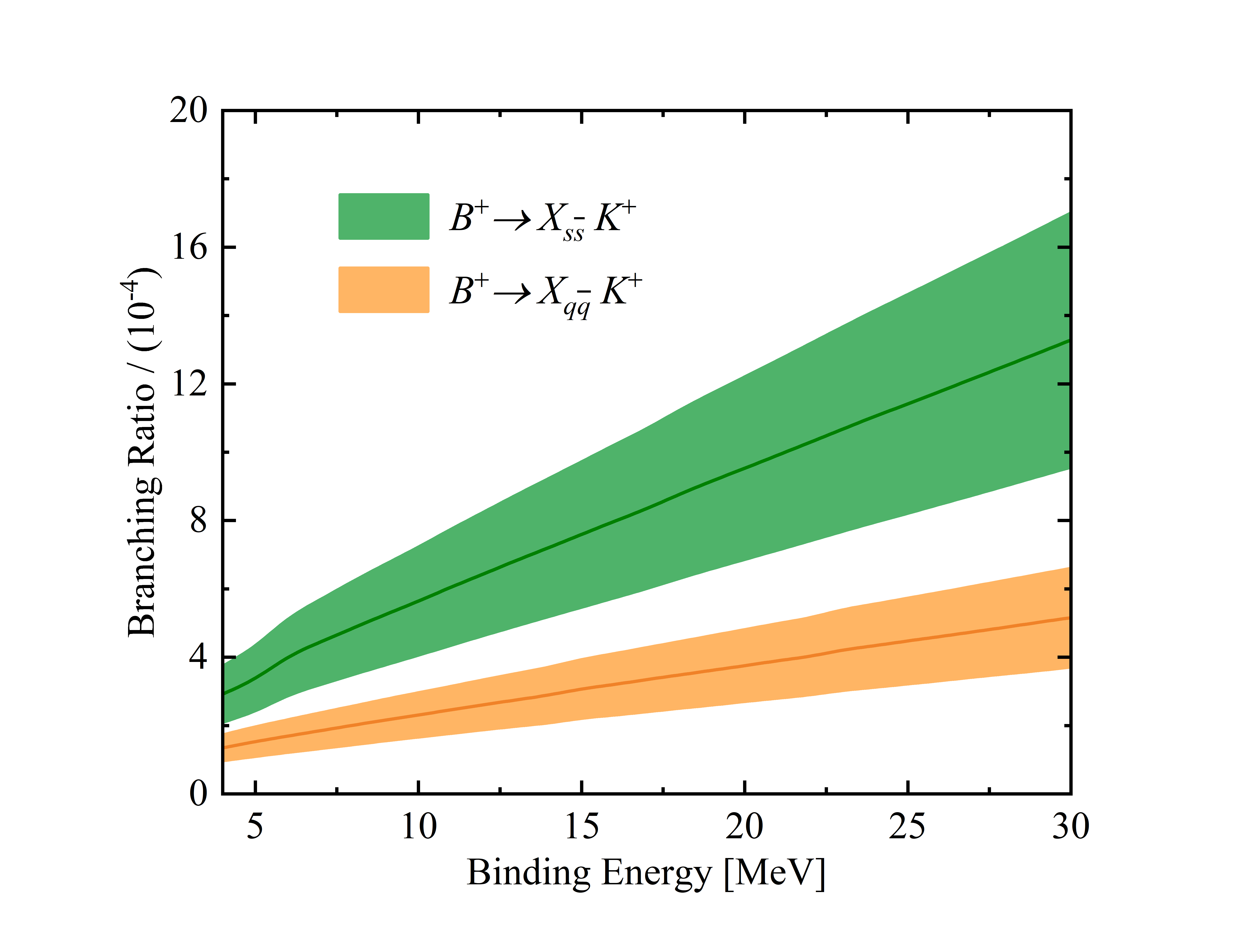
Figure 3: Branching ratios of $B^{+}\to X_{s\bar{s}}K^{+}$ and $B^{+}\to X_{q\bar{q}}K^{+}$ as functions of the binding energies of $D_{s}^{+}D_{s}^{-}$ and $\bar{D}D$ bound states

For the $\bar{D}D$ bound state, we determine the coupling of $g_{X_{q\bar{q}}\bar{D}D}$ as $9.62\sim 19.38$ GeV. The coupling of $g_{X_{q\bar{q}}\bar{D}^{0}D^{0}}$ is further determined by the isospin symmetry, i.e., $g_{X_{q\bar{q}}\bar{D}^{0}D^{0}}=\frac{1}{\sqrt{2}}g_{X_{q\bar{q}}\bar{D}D}$. With the couplings so obtained we calculate the branching ratio of $B^{+}\to X_{q\bar{q}}K^{+}$, which turns out to be in the range of $(1.3{\pm 0.4}\sim 5.2{\pm 1.5})\times 10^{-4}$ as shown in Fig. 3. We note that the only allowed strong decay mode of a $\bar{D}D$ isoscalar molecule is $\eta_{c}\eta$, which implies that the branching ratio of $B^{+}\to(X_{q\bar{q}}\to\eta_{c}\eta)K^{+}$ is $10^{-4}$, which agrees well with the upper limit of the branching ratio of $B^{+}\to\eta_{c}\eta K^{+}$, $2.2\times 10^{-4}$ Zyla et al. (2020). Therefore, our result indicates that the $\bar{D}D$ bound state can be detected in the $\eta_{c}\eta$ mass distribution of the $B^{+}\to\eta_{c}\eta K^{+}$ decay.

At last, we study the scenario where $X_{s\bar{s}}$ is a resonant state of $D_{s}^{+}D_{s}^{-}$, which can be identified as the $X(3960)$ state recently discovered by the LHCb Collaboration. Here we assume that $X(3960)$ is dynamically generated by the $D_{s}^{+}D_{s}^{-}$ interaction. With a contact potential of the form $C_{a}$ + $C_{b}q^{2}$, one can reproduce the mass and width of $X(3960)$ by solving the Lippmann-Schwinger equation Zhai et al. (2022), and then obtain the $X(3960)$ coupling to $D_{s}^{+}D_{s}^{-}$ from the residues of the pole Xie et al. (2022), where $C_{a}$ and $C_{b}$ are two low energy constants, and $q$ is the momentum of $D_{s}^{\pm}$ in the center-of-mass system of the $D_{s}^{+}D_{s}^{-}$ pair. With the experimental mass and width of $X(3960)$ as input, we obtain $C_{a}=-5.15$ GeV^-2 and $C_{b}=-148.55$ GeV^-4 for a cutoff of $\Lambda=1$ GeV, and then determine the coupling $g_{X_{s\bar{s}}D_{s}^{+}D_{s}^{-}}=7.87$ GeV. With the so-determined coupling we calculate the branching ratio of $B^{+}\to X_{s\bar{s}}K^{+}$ and obtain $(1.9{\pm 0.5})\times 10^{-4}$.

IV Summary and Discussion

The recently discovered $X(3960)$ by the LHCb Collaboration motivated us to study the $D_{s}^{+}D_{s}^{-}$ and $\bar{D}D$ molecules predicted in a number of recent works. In this work, we assumed that there exist two bound states below the mass thresholds of $D_{s}^{+}D_{s}^{-}$ and $\bar{D}D$, respectively, and studied their production in the $B$ decays via the triangle mechanism. In such a mechanism, $B^{+}$ first weakly decays into $D_{s}^{+}\bar{D}^{\ast 0}$ and $D_{s}^{\ast+}\bar{D}^{0}$, the $\bar{D}^{*0}$/$D_{s}^{*+}$ decays into $D_{s}^{-}$/$D^{0}$ plus a kaon, and then the final state $D_{s}^{+}D_{s}^{-}$ and $\bar{D}^{0}{D}^{0}$ interactions dynamically generate the $X_{s\bar{s}}$ and $X_{q\bar{q}}$ molecules. As for the bound states, we employed the compositeness condition approach to determine their couplings to their constituents. The resonant state of $D_{s}^{+}D_{s}^{-}$ is dynamically generated in the single-channel approximation, and the corresponding coupling is determined from the residues of the pole.

We employed the effective Lagrangian approach to calculate the branching ratios of $B^{+}\to X_{s\bar{s}}K^{+}$ and $B^{+}\to X_{q\bar{q}}K^{+}$ assuming that $X_{s\bar{s}}$ and $X_{q\bar{q}}$ are bound states and found that both of them are of the order of $10^{-4}$. Our results indicate that such bound states of $\bar{D}D$ and $D_{s}^{+}D_{s}^{-}$ (if exist) have large production rates in the $B$ decays since they account for a large portion of the relevant experimental data as shown in Table 2. We note that the $\bar{D}D$ bound state is likely to be detected in the $\eta_{c}\eta$ mass distribution of the $B^{+}\to\eta_{c}\eta K^{+}$ decay since the $\bar{D}D$ bound state only decays into $\eta_{c}\eta$, while the $D_{s}^{+}D_{s}^{-}$ bound state has more decay modes, e.g., $B^{+}\to\bar{D}DK^{+}$, $B^{+}\to\eta_{c}\eta K^{+}$, and $B^{+}\to J/\psi\omega K^{+}$. At last, assuming that the $X(3960)$ state is dynamically generated by the $D_{s}^{+}D_{s}^{-}$ single-channel interaction, we obtained the branching ratio of $B^{+}\to X(3960)K^{+}=(1.9{\pm 0.5})\times 10^{-4}$, which can help elucidate the nature of $X(3960)$.

Table 2: Branching ratios of $B\to X_{s\bar{s}/q\bar{q}}/X(3960)K^{+}$ where $X_{s\bar{s}/q\bar{q}}$ is a bound state of $D_{s}^{+}D_{s}^{-}$ or $\bar{D}D$.

Decay modes	Our results	Exp Zyla et al. (2020)
$B^{+}\to X_{s\bar{s}}K^{+}$	$({2.1\sim 17.0})\times 10^{-4}$	$\mathrm{Br}(B^{+}\to\chi_{c0}(3915)K^{+})<2.8\times 10^{-4}$
$B^{+}\to(X_{q\bar{q}}\to\eta_{c}\eta)K^{+}$	$({0.9\sim 6.7})\times 10^{-4}$	$\mathrm{Br}(B^{+}\to\eta_{c}\eta K^{+})<2.2\times 10^{-4}$
$B^{+}\to X(3960)K^{+}$	$<{2.4}\times 10^{-4}$	-

V Acknowledgments

This work is supported in part by the National Natural Science Foundation of China under Grants No.11975041, No.11735003, and No.11961141004. Ming-Zhu Liu acknowledges support from the National Natural Science Foundation of China under Grant No.12105007 and China Postdoctoral Science Foundation under Grants No. 2022M710317, and No.2022T150036.

References

- Abe et al. (2005) K. Abe et al. (Belle), Phys. Rev. Lett. 94, 182002 (2005), arXiv:hep-ex/0408126 .
- Aubert et al. (2008) B. Aubert et al. (BaBar), Phys. Rev. Lett. 101, 082001 (2008), arXiv:0711.2047 [hep-ex] .
- Uehara et al. (2010) S. Uehara et al. (Belle), Phys. Rev. Lett. 104, 092001 (2010), arXiv:0912.4451 [hep-ex] .
- Lees et al. (2012) J. P. Lees et al. (BaBar), Phys. Rev. D 86, 072002 (2012), arXiv:1207.2651 [hep-ex] .
- Aaij et al. (2020a) R. Aaij et al. (LHCb), Phys. Rev. D 102, 112003 (2020a), arXiv:2009.00026 [hep-ex] .
- Aaij et al. (2020b) R. Aaij et al. (LHCb), Phys. Rev. Lett. 125, 242001 (2020b), arXiv:2009.00025 [hep-ex] .
- Zyla et al. (2020) P. A. Zyla et al. (Particle Data Group), PTEP 2020, 083C01 (2020).
- Duan et al. (2020) M.-X. Duan, S.-Q. Luo, X. Liu, and T. Matsuki, Phys. Rev. D 101, 054029 (2020), arXiv:2002.03311 [hep-ph] .
- Duan et al. (2021) M.-X. Duan, J.-Z. Wang, Y.-S. Li, and X. Liu, Phys. Rev. D 104, 034035 (2021), arXiv:2104.09132 [hep-ph] .
- LHC (2022a) (2022a), arXiv:2210.15153 [hep-ex] .
- LHC (2022b) (2022b), arXiv:2211.05034 [hep-ex] .
- Barnes et al. (2005) T. Barnes, S. Godfrey, and E. S. Swanson, Phys. Rev. D 72, 054026 (2005), arXiv:hep-ph/0505002 .
- Li and Chao (2009) B.-Q. Li and K.-T. Chao, Phys. Rev. D 79, 094004 (2009), arXiv:0903.5506 [hep-ph] .
- Bayar et al. (2022) M. Bayar, A. Feijoo, and E. Oset, (2022), arXiv:2207.08490 [hep-ph] .
- Xin et al. (2022) Q. Xin, Z.-G. Wang, and X.-S. Yang, (2022), arXiv:2207.09910 [hep-ph] .
- Ji et al. (2022) T. Ji, X.-K. Dong, M. Albaladejo, M.-L. Du, F.-K. Guo, and J. Nieves, (2022), arXiv:2207.08563 [hep-ph] .
- Prelovsek et al. (2021) S. Prelovsek, S. Collins, D. Mohler, M. Padmanath, and S. Piemonte, JHEP 06, 035 (2021), arXiv:2011.02542 [hep-lat] .
- Gamermann et al. (2007) D. Gamermann, E. Oset, D. Strottman, and M. J. Vicente Vacas, Phys. Rev. D 76, 074016 (2007), arXiv:hep-ph/0612179 .
- Liu et al. (2019) M.-Z. Liu, T.-W. Wu, M. Pavon Valderrama, J.-J. Xie, and L.-S. Geng, Phys. Rev. D 99, 094018 (2019), arXiv:1902.03044 [hep-ph] .
- Wu et al. (2021) T.-W. Wu, M.-Z. Liu, and L.-S. Geng, Phys. Rev. D 103, L031501 (2021), arXiv:2012.01134 [hep-ph] .
- Liu and Geng (2021) M.-Z. Liu and L.-S. Geng, Eur. Phys. J. C 81, 179 (2021), arXiv:2012.05096 [hep-ph] .
- Dong et al. (2021) X.-K. Dong, F.-K. Guo, and B.-S. Zou, Progr. Phys. 41, 65 (2021), arXiv:2101.01021 [hep-ph] .
- Peng et al. (2022) F.-Z. Peng, M. Sánchez Sánchez, M.-J. Yan, and M. Pavon Valderrama, Phys. Rev. D 105, 034028 (2022), arXiv:2101.07213 [hep-ph] .
- Wang et al. (2021a) E. Wang, H.-S. Li, W.-H. Liang, and E. Oset, Phys. Rev. D 103, 054008 (2021a), arXiv:2010.15431 [hep-ph] .
- Deineka et al. (2022) O. Deineka, I. Danilkin, and M. Vanderhaeghen, Phys. Lett. B 827, 136982 (2022), arXiv:2111.15033 [hep-ph] .
- Dai et al. (2016) L. R. Dai, J.-J. Xie, and E. Oset, Eur. Phys. J. C 76, 121 (2016), arXiv:1512.04048 [hep-ph] .
- Li and Voloshin (2015) X. Li and M. B. Voloshin, Phys. Rev. D 91, 114014 (2015), arXiv:1503.04431 [hep-ph] .
- Wu and Chen (2019) Q. Wu and D.-Y. Chen, Phys. Rev. D 100, 114002 (2019), arXiv:1906.02480 [hep-ph] .
- Lu et al. (2021) J.-X. Lu, M.-Z. Liu, R.-X. Shi, and L.-S. Geng, Phys. Rev. D 104, 034022 (2021), arXiv:2104.10303 [hep-ph] .
- Cheng et al. (2005) H.-Y. Cheng, C.-K. Chua, and A. Soni, Phys. Rev. D 71, 014030 (2005), arXiv:hep-ph/0409317 .
- Cheng and Yang (2008) H.-Y. Cheng and K.-C. Yang, Phys. Rev. D 78, 094001 (2008), [Erratum: Phys.Rev.D 79, 039903 (2009)], arXiv:0805.0329 [hep-ph] .
- Chen (2022) H.-X. Chen, Phys. Rev. D 105, 094003 (2022), arXiv:2103.08586 [hep-ph] .
- Wang et al. (2021b) F.-L. Wang, X.-D. Yang, R. Chen, and X. Liu, Phys. Rev. D 104, 094010 (2021b), arXiv:2103.04698 [hep-ph] .
- Buras (1998) A. J. Buras, “Weak hamiltonian, cp violation and rare decays,” (1998).
- Geng et al. (2018) C. Q. Geng, Y. K. Hsiao, Y.-H. Lin, and L.-L. Liu, Phys. Lett. B 776, 265 (2018), arXiv:1708.02460 [hep-ph] .
- Han et al. (2021) J.-J. Han, H.-Y. Jiang, W. Liu, Z.-J. Xiao, and F.-S. Yu, Chin. Phys. C 45, 053105 (2021), arXiv:2101.12019 [hep-ph] .
- Ali et al. (1998) A. Ali, G. Kramer, and C.-D. Lu, Phys. Rev. D 58, 094009 (1998), arXiv:hep-ph/9804363 .
- Qin et al. (2014) Q. Qin, H.-n. Li, C.-D. Lü, and F.-S. Yu, Phys. Rev. D 89, 054006 (2014), arXiv:1305.7021 [hep-ph] .
- Bauer et al. (1987) M. Bauer, B. Stech, and M. Wirbel, Z. Phys. C 34, 103 (1987).
- Verma (2012) R. C. Verma, J. Phys. G 39, 025005 (2012), arXiv:1103.2973 [hep-ph] .
- Arrington et al. (2007) J. Arrington, C. D. Roberts, and J. M. Zanotti, J. Phys. G 34, S23 (2007), arXiv:nucl-th/0611050 .
- Punjabi et al. (2015) V. Punjabi, C. F. Perdrisat, M. K. Jones, E. J. Brash, and C. E. Carlson, Eur. Phys. J. A 51, 79 (2015), arXiv:1503.01452 [nucl-ex] .
- Collins et al. (2011) S. Collins et al., Phys. Rev. D 84, 074507 (2011), arXiv:1106.3580 [hep-lat] .
- Can et al. (2014) K. U. Can, G. Erkol, B. Isildak, M. Oka, and T. T. Takahashi, JHEP 05, 125 (2014), arXiv:1310.5915 [hep-lat] .
- Ling et al. (2021a) X.-Z. Ling, J.-X. Lu, M.-Z. Liu, and L.-S. Geng, Phys. Rev. D 104, 074022 (2021a), arXiv:2106.12250 [hep-ph] .
- Ling et al. (2022) X.-Z. Ling, M.-Z. Liu, L.-S. Geng, E. Wang, and J.-J. Xie, Phys. Lett. B 826, 136897 (2022), arXiv:2108.00947 [hep-ph] .
- Weinberg (1963) S. Weinberg, Phys. Rev. 130, 776 (1963).
- Salam (1962) A. Salam, Nuovo Cim. 25, 224 (1962).
- Hayashi et al. (1967) K. Hayashi, M. Hirayama, T. Muta, N. Seto, and T. Shirafuji, Fortsch. Phys. 15, 625 (1967).
- Aoki et al. (2020) S. Aoki et al. (Flavour Lattice Averaging Group), Eur. Phys. J. C 80, 113 (2020), arXiv:1902.08191 [hep-lat] .
- Donald et al. (2012) G. C. Donald, C. T. H. Davies, R. J. Dowdall, E. Follana, K. Hornbostel, J. Koponen, G. P. Lepage, and C. McNeile, Phys. Rev. D 86, 094501 (2012), arXiv:1208.2855 [hep-lat] .
- Li et al. (2017) Y. Li, P. Maris, and J. P. Vary, Phys. Rev. D 96, 016022 (2017), arXiv:1704.06968 [hep-ph] .
- Dürr et al. (2017) S. Dürr et al., Phys. Rev. D 95, 054513 (2017), arXiv:1601.05998 [hep-lat] .
- Miller et al. (2020) N. Miller et al., Phys. Rev. D 102, 034507 (2020), arXiv:2005.04795 [hep-lat] .
- Faessler et al. (2007a) A. Faessler, T. Gutsche, V. E. Lyubovitskij, and Y.-L. Ma, Phys. Rev. D 76, 014005 (2007a), arXiv:0705.0254 [hep-ph] .
- Faessler et al. (2007b) A. Faessler, T. Gutsche, S. Kovalenko, and V. E. Lyubovitskij, Phys. Rev. D 76, 014003 (2007b), arXiv:0705.0892 [hep-ph] .
- Ling et al. (2021b) X.-Z. Ling, M.-Z. Liu, and L.-S. Geng, Eur. Phys. J. C 81, 1090 (2021b), arXiv:2110.13792 [hep-ph] .
- Zhai et al. (2022) Q.-Y. Zhai, M.-Z. Liu, J.-X. Lu, and L.-S. Geng, Phys. Rev. D 106, 034026 (2022), arXiv:2205.03878 [hep-ph] .
- Xie et al. (2022) J.-M. Xie, X.-Z. Ling, M.-Z. Liu, and L.-S. Geng, (2022), arXiv:2204.12356 [hep-ph] .