Optimal Convergence Rates of Deep Neural Networks in a Classification Setting
Abstract
We establish optimal convergence rates up to a -factor for a class of deep neural networks in a classification setting under a restraint sometimes referred to as the Tsybakov noise condition. We construct classifiers in a general setting where the boundary of the bayes-rule can be approximated well by neural networks. Corresponding rates of convergence are proven with respect to the misclassification error. It is then shown that these rates are optimal in the minimax sense if the boundary satisfies a smoothness condition. Non-optimal convergence rates already exist for this setting. Our main contribution lies in improving existing rates and showing optimality, which was an open problem. Furthermore, we show almost optimal rates under some additional restraints which circumvent the curse of dimensionality. For our analysis we require a condition which gives new insight on the restraint used. In a sense it acts as a requirement for the ”correct noise exponent” for a class of functions.
| Keywords: Tsybakov noise condition, Classification using deep neural |
| networks |
| MSC2020 subject classifications: 62C20, 62G05. |
1 Introduction
We consider i.i.d. data with and . Our goal is to provide an estimator of the form where is constructed with a neural network which approximates well with respect to the misclassification error. We show optimal convergence rates under the following two conditions. First, the underlying distribution satisfies a noise condition as in [22] described below. Second, the boundary of the set
with satisfies certain regularity conditions.
Neural Networks have shown outstanding results in many classification tasks such as image recognition [7], language recognition [4], cancer recognition [10], and other disease detection [16]. Our work follows current approaches in the statistical literature to explain the success of neural networks, e.g. the impactful contributions [12, 21]. The objective is to fill a gap in the literature by proving optimal convergence rates in a specific setting which was also considered in [11]. We focus on deep feedforward neural networks with ReLU-activation functions. Deep networks have been considered in many theoretical articles [12, 13, 18, 19] and have proven useful in many applications [20, 15]. Intuitively, we wish to approximate the set directly instead of approximating the regression function . The classification setting we consider is similar to the setting given in [17, 22]. In particular, we assume that satisfies a noise condition which can be described as follows. For -measurable sets define
The condition then states that there exists a constant such that
| (1.1) |
for some constant and all . This requirement is sometimes referred to as the Tsybakov noice condition. It can be interpreted as a restraint on the probability distribution regarding regions close to the boundary where . Roughly speaking, it forces the mass to decay at a certain rate when one approaches this boundary. Using this, one can achieve rates approaching for small , i.e. if there is not much mass in the region around . The condition has been used in many statistical articles considering classification such as [1] and [23] who analyse support vector machines. Similarly to [17], we show optimal convergence rates in the case where the boundary of satisfies certain regularity conditions, i.e. is similar to an element of a Dudley class [6]. More precisely, we consider sets which are slightly more general then the sets given in [18]. While many other approximation results using neural networks exist, see [5] using sigmoid activation functions or [24] using piecewise linear functions among others, the methods used in [18] inspired us to obtain the results for our setting. The sets they consider have been used in many articles such as [11, 19]. As an estimator, we use a risk minimizer of the empirical version of the misclassification error. Precisely calculating this estimator involves finding a global minimum of a highly non-convex loss with respect to the parameters of a neural network. Typically, such calculations are not feasible in practice. Thus, the results we provide are theoretical in nature and do not have direct useful applications, as is typical for results of this kind [13, 21]. From our point of view, the main value of current contributions is to show results such as consistency in situations which are typical for statisticians using relatively simple classes of neural networks. In time, the techniques developed may be used to show claims in cases which are closer to those encountered in reality and using classes of neural networks which are closer to those used in practise.
A lot of work has been done regarding consistency of feedforward deep neural networks. [21] prove optimal convergence rates with respect to the uniform norm in a regression setting. Among others, similar results were given by [9] for non-continuous regression functions with respect to the -norm, [14] who did not use a sparsity constraint, and [2]. Regarding results for classification, [19] show convergence rates considering the misclassification error in a noiseless setting. Consistency results which include condition (1.1) in the assumptions are given by [3, 13, 8]. In contrast to our approach, the previously mentioned articles attempt to estimate the regression function instead of directly estimating the set . Additionally, while some obtain optimal convergence rates, the settings do not correspond to the setting given in [22]. In particular, the (optimal) convergence rates differ from ours in these papers. A very interesting contribution was made by [11] who consider an almost identical situation to ours, while their estimators differ. However, the rates they obtain are not optimal in the minimax sense.
1.1 Contribution
Our contribution includes the following.
-
•
First and foremost, Theorem 4.1 together with Corollary 3.7 prove optimal convergence rates in the minimax sense for the setting described above. To the best of our knowledge, we are the first to obtain optimal convergence rates using neural networks corresponding to the setting given in [22] and thus close this gap in the literature.
-
•
Theorem 3.5 establishes convergence rates in a general setting, where the boundary of the set can be well approximated by neural networks. This enables us to prove rates in a variety of settings. We use this theorem to prove optimal convergence rates under an additional constraint, which circumvents the curse of dimensionality, in the sense that the rates do not decrease exponentially in the dimension .
- •
1.2 Outline
After introducing some notation, we rigorously introduce the problem at hand in Section 2. Here, we also provide some convergence results considering empirical risk minimizers with respect to arbitrary sets. These results are then used to prove our main consistency theorems regarding neural networks in Section 3. Section 4 includes the corresponding lower bounds followed by some concluding remarks in Section 5.
1.3 Notation
We introduce some general notation which is used throughout this article.
For , let and . Let be the Lebesgue measure. For a function and denote by
the uniform-norm and the -norm, respectively. Note that we omit the dependence on in the notation. For , let and be the euclidean-norm and the uniform-norm, respectively. For let
Additionally, let
For let .
Now, let . Define and . For let
be the Hoelder-norm. For , define the class of Hoelder-continuous functions by
Let be two subsets. We write
for their symmetric difference and
for the indicator function corresponding to .
2 General Convergence Results
In this section, we state our results in a relatively general setting. The results on neural networks in the next section only consider the case where has a bounded density with respect to the Lebesgue measure. Our setup is similar to the binary classification setup of [22].
2.1 Classification Setup
Let be observations distributed according to some probability measure , where and . Denote by the marginal probability distribution with respect to . The goal is to predict when observing , where is distributed according to independently of using classifiers of the form
for some -measurable set . Note that a classifier is uniquely determined by . Performance is measured by the misclassification error
For the set
is a so called bayes rule and thus minimizes the misclassification error. Classification can equivalently be seen as estimation of by the set , which is therefore equally referred to as classifier. For a -measureable set let
be the empirical version of the misclassification error . We consider empirical risk minimization classifiers defined by
where is some finite collection of -measurable sets for all .
2.2 Consistency Results
Proposition 2.1 establishes convergences rates for estimating using under certain conditions on and . For the loss function, we consider a slight generalization of the misclassification error
for . The proposition is somewhat similar to Theorem 2 from [17]. In contrast to our approach, they consider the discrimination of two probability distributions with underlying distribution functions and do not allow for non-optimal convergence rates. The proposition is an important component for the proof of our main theorem given in Section 3. The proofs of this section can be found in Appendix A.
Proposition 2.1.
Let be a monotonically increasing sequence. Let be a class of potential joint distributions of and be a collection of subsets of for all such that the following conditions hold.
-
(i)
For all all sets in and are -measurable.
-
(ii)
There exists a constant such that
for some constant , all and all .
Additionally, we assume that there is a constant such that for all the following holds.
-
(iii)
There is a constant such that for all there is a with
-
(iv)
There exist constants such that
Then for all we have
where
for all .
Condition (i) is needed for all terms to be well defined. Condition (iii) states that the set in question must be well approximated by elements of . A sufficient assumption is that is an -net of ,
where . Together with (iv), this indirectly bounds the complexity of . If the class of sets is to large, one will not be able to find sets that satisfy (iii) and (iv) at the same time. It is clear that the best rates are achieved with . We do not use the same sequences in conditions (iii) and (iv) since one can prove non-optimal convergence rates using this version of the proposition.
The second condition is the noise condition described in the introduction. Note that following [22], for condition (ii) holds if
for all and some . Roughly speaking, this forces the mass to decay at a certain rate when one approaches the boundary of . Note that we use (ii) instead of this assumption since it is slightly more general and includes the case . Additionally, it appears more naturally in the proofs. Observing the alternative assumption, corresponds to the case where there is no mass close to the boundary of , meaning that does not take on values close to . Using Proposition 2.1 one can achieve rates approaching for small i.e. if there is not much mass in the region around and the complexity of , and consequently , is moderate. In contrast, the following proposition provides convergence rates if condition (ii) is not satisfied.
Proposition 2.2.
Let be a monotonically increasing sequence. Let be a class of potential joint distributions of and be a collection of subsets of for all such that the following conditions hold.
-
(i)
For all all sets in and are -measurable.
Additionally, we assume that there is a constant such that for all the following holds.
-
(ii)
There is a constant such that for all and there is a with
-
(iii)
There exist such that
Then for all we have
where
for all .
Note that the requirement in conditon (ii) of Proposition 2.2 corresponds to requirement (iii) of 2.1 with . However, for the best rate achievable is of order , which is always slower . Proposition 2.2 provides rates in absence of condition (ii) of Proposition 2.1. We do not claim optimality for these rates.
3 Convergence Rates for Neural Networks
We begin by shortly introducing neural networks. The idea is to use Proposition 2.1 to obtain optimal convergence rates up to a log factor. Neural networks are used to define a suitable class of sets for every .
3.1 Definitions regarding Neural Networks
Definition 3.1.
Let . For , let be a function
For , define a shifted -dimensional version of by
A neural network with network architecture
is a sequence
where each is a weight matrix and is a shift vector. The realization of a neural network on a set is the function
We denote by
the set of realizations of neural networks with network architecture , where and .
Typically, for the function is called activation function and is named shifted activation function. The constant denotes the number of hidden Layers. The values and are the input and output dimensions, respectively. In this article, we are interested in the case where for the activation function in the -th layer is the rectifier linear unit (ReLU)
Additionally, if not further specified, we consider a compact domain and a one dimensional output . For the sake of completeness, we note that a network with L=0 layers is of the form for and has realization . Note that, in general, the weights of a neural network , i.e. the entries of its shift vectors and weight matrices , are not uniquely determined by its realization . In the following, for brevity, we occasionally introduce a network by defining its realization. In such a case, it is clear from the presentation of the realization which precise neural network is considered.
As a first step, we wish to introduce a suitable finite class of sets parameterized by neural networks and count the number of elements. We define these sets as where is a realization of a neural network. Equivalently, we could have considered neural networks with a binary step function in the output layer or find a neural network and define the approximating set , which is closer to the idea that the realization of the neural network represents some sort of probability. Since this is not the idea of our approximation results, we stick to the version above. In order to obtain a finite class, we need to reduce the number of considered elements of while maintaining reasonable approximating capabilities. A typical approach in the theoretical literature is to use a sparsity constraint. For we therefore only consider realizations of neural nets which have at most nonzero weights. If is the total number of nonzero weights, we say that the network has sparsity . Additionally, we assume all weights to be elements of the set
Thus, we only consider weights . Concluding, we use the following notation to describe the collection of sets we are interested in.
Definition 3.2.
Let and be fixed. Denote by the set of realizations of neural networks with dimensional input, one dimensional output, at most layers, ReLU activation functions and sparsity at most , where all weights are elements of . The class of corresponding sets given by neural networks is then
Note that the requirements from Definition 3.2 allow for realizations of neural networks with arbitrary hidden layer dimensions . However, it is easy to see that every element of is a realization of a neural net which satisfies the properties described in the Definition and for all . Using this, we receive an upper bound on the number of elements of by counting the number of corresponding neural networks. Thus, the following bound is independent of the choice of activation functions .
Lemma 3.3.
For and let be the class of sets introduced in Definition 3.2. We have an upper bound on the number of elements given by
Proof.
First of all, if , clearly only the last layers have influence on the realization of a neural network. Thus, an upper bound is given by counting the number of neural nets with at most layers, at most sparsity , weights in and for all . Each weight can take on different values. The total number of weights can be bounded by
Note that if , the input dimension does not influence the outcome. Therefore, there are at most
possible combinations to pick (possibly) nonzero weights. Thus
∎
3.2 Conditions on the Bayes-Rule
In order to define the set of probability distributions we consider for approximation, we restrict the possible bayes rules. We then add a smoothness condition to the function near the boundary of the respective bayes rule. Intuitively, the boundary should satisfy some kind of smoothness condition so that it can be approximated by neural networks. Additionally, the set must be discretizable in some sense. When using the class of sets we use is similar to a class defined in [18]. Note, that the class used here is larger. This version depends on a set which represents a class of boundary functions. The idea is that we can obtain different convergence rates for different classes using the same procedure.
Definition 3.4.
Let , and with . Additionally, let , , be a probability measure on and be a class of functions
Define
and
if . Let be the class of all subsets for such that for there exist with the following properties.
-
1.
For all we have
-
2.
for .
-
3.
If , the following holds. For and all there exists such that for we have
where .
-
4.
for all .
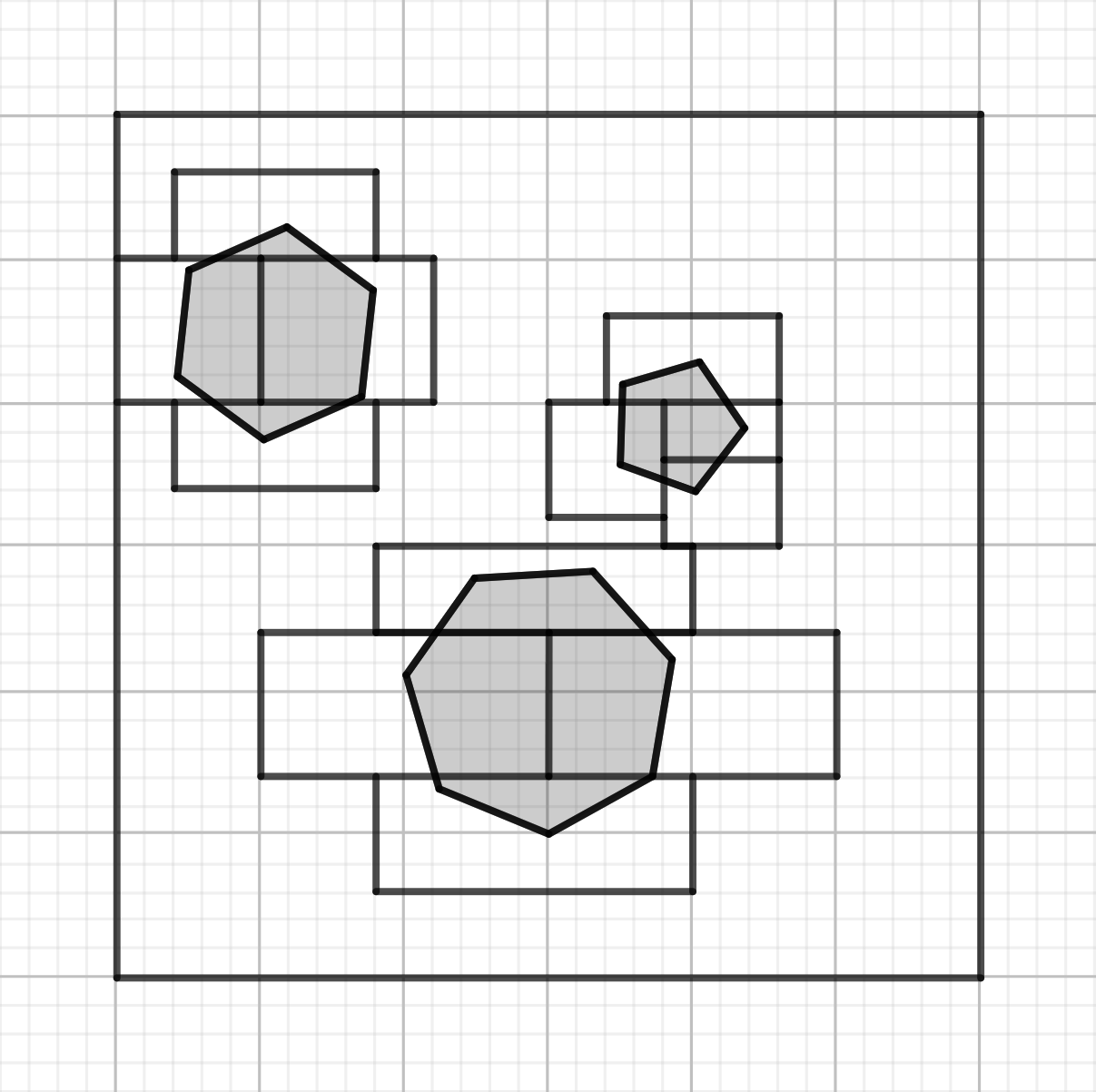
Note that implies . The idea is to use sets defined by realizations of neural networks to approximate from Definition 3.4 for a suitable class in order to apply Proposition 2.1. Figure 1 shows an example for an element of , where is the set of piecewise linear functions. The definition contains an additional condition on the function close to the boundary of . Following the intuition mentioned in [17], for condition (ii) in Theorem 2.1 means that acts like close to the boundary of , where . More precisely, condition (ii) requires that does not increase slower than . In order to prove the combination of conditions (iii) and (iv), we require that is the correct rate, meaning that does not increase faster than . In Section 4 we prove that this condition does not lower the complexity of the problem. Thus, the rates obtained by [17] are still optimal.
3.3 Main Theorems
We begin by stating the central result of this article. We then use this result to show consistency results for more specific cases. The rates we obtain in Theorem 3.5 are optimal up to a factor. In the following, all proofs of this section are given in Appendix B.
Theorem 3.5.
Let , and with . Let be a set of functions
such that the following holds. There exist and such that for any and any there is a neural network with layers, sparsity and weights in with such that
Define and let be a class of potential joint distributions of such that the following conditions hold.
-
(a)
There is a constant such that for all the marginal distribution of has a Lebesgue density bounded by .
-
(b)
There are constants and such that for all the bayes rule satisfies .
-
(c)
We have
for some constant , all and all , where
is the class of sets corresponding to any neural network.
Let
Then there exist constants and such that for all we have
where
with .
3.4 Results for Regular Boundaries
We can now prove results for specific classes of sets to obtain convergence results. A first important example is the class . The following Lemma is a consequence of Theorem 5 in [21].
Lemma 3.6.
Let and . Then there exist such that the following holds. For any function and any , there exists a neural network with layers, sparsity and weights in with such that
Corollary 3.7.
Corollary 3.7 together with Theorem 4.1 from the next chapter prove optimal convergence rates, which was the main goal of this paper.
Following up, note that the rates we receive from Corollary 3.7 are affected by the curse of dimensionality. Observe that the rates obtained by Theorem 3.5 are influenced by condition (c) on the one hand and the ability of neural networks to approximate sets in on the other. The dependence on the dimension in Corollary 3.7 comes from the latter. Thus, a natural approach to circumvent the curse of dimensionality is to approximate a smaller set . Intuitively, it is clear that without strong restrictions on the distribution we can only overcome the curse if the complexity of the boarders of the sets we approximate is small enough so that they themselves can overcome the curse. In the literature, many different sets are considered which infer useful approximation capabilities of neural networks. Here, we use a class of sets introduced by [21] which is close to class .
Definition 3.8.
Let , , , and with , for , . Define
where
Instead of requiring that is supported on , we could have used the condition that is supported on for some values . However, this does not enlarge the class considerably. It can easily be seen that we can instead increase the bound to find an even larger class. The idea for using the set is that its complexity does not depend on the input dimension , but only on the most difficult component to approximate. The complexity of the components depend on their effective dimension and their implied smoothness. As described by [21], the correct smoothness parameter to consider is
Examples for sets that can profit from Definition 3.8 are additive models (, ), interaction models of order (, ), or multiplicative models (they are a subset of when , for all ). Next, our goal is to establish a convergence result when the set of boundary functions is . Similarly to the approach above, we first provide a lemma which provides approximation results using neural networks.
Lemma 3.9.
Let , , , and with , for , . Let be defined as in Definition 3.8 and define
Then there exist such that the following holds. For any function and any , there exists a neural network with layers, sparsity and weights in with such that
The following corollary establishes the corresponding convergence result. Theorem 4.2 provides the lower bound in the case where .
Corollary 3.10.
Let , , , , , and with for , . Additionally, and for . Define with , for and
Define and let be a class of potential joint distributions of such that the following conditions hold.
-
(a)
There is a constant such that for all the marginal distribution of has a Lebesgue density bounded by .
-
(b)
There are constants and such that for all the bayes rule satisfies with
-
(c)
We have
for some constant , all and all , where
is the class of sets corresponding to any neural network.
Let
Then there exist constants and such that for all we have
where
with .
4 Lower Bound
We now establish lower bounds on the convergence rates from corollaries 3.7 and 3.10. Note that the lower bounds also prove that the rates obtained in Theorem 3.5 can not be improved up to a -factor. Since Corollary 3.10 is a generalisation of 3.7, we only have to prove a lower bound for the setting given in the former. For clarity, we provide both statements. The proofs of this section can be found in Appendix C.
Theorem 4.1.
Let , and with . Let be the class of all potential joint distributions of such that (a),(b) from Theorem 3.5 hold with , , , , and some , , . Let (c) hold with large enough and set
Then
for every , where contains all estimators depending on the data .
Intuitively, bounds the factor of the -term of close to the boundary from above. On the other hand, bounds this term from below. Thus, not every combination of is possible. We prove Theorem 4.1 for large . We do not provide the exact ratio of and required since it is not important for the statement. Lastly, the lower bound corresponding to Corollary 3.10 is given.
Theorem 4.2.
Let , , , , , and with for , . Additionally, and for . Let
Define and let be the class of all potential joint distributions of such that (a),(b) from Corollary 3.10 hold for some , , . Let (c) hold with large enough and set
Then
for every , where contains all estimators depending on the data .
5 Concluding Remarks
We establish optimal convergence rates up to a -factor in a classification setting under the (1.1) using neural networks. Theorem 3.5 can be applied for many different boundary functions. The complexity of the class of boundary functions is one of the main driving factors of the convergence rate. In particular, many approaches which circumvent the curse of dimensionality in a regression setting can be used to circumvent the curse in this classification setting.
Note that this paper is of a theoretical nature. While sparsity constraints are considered thoroughly in the theoretical literature, they are not widely used in practice. Additionally, we did not discuss the minimization required for the calculation of . This is a very interesting but complicated topic which is not in the scope of this article. Observe that the class of neural networks used in Theorem 3.5 depends on as well as . We believe that one can extend the results of this paper by either having adaptive classes of neural networks or a class independent of and in a similar manner to [22]. One obstacle to overcome is the fact that the conditions on the probability distribution required are not strictly weaker for larger and .
Lastly, while the goal of this paper is to prove results considering neural networks, it also contains new insights on the noise condition (1.1). In order to establish optimal convergence, an additional condition in order to show approximation results of neural networks with respect to the metric is necessary. Intuitively, the reverse inequality is required for certain sets. Note that requiring the reverse inequality is an overly restrictive assumption which holds for almost no classes of possible distributions for . This proved to be a major challenge and is solved by (3.) in Definition 3.4. While this condition is always also satisfied for larger but not lower (and thus ), the reverse is true in condition (1.1). Thus, together the requirement is that is the ”correct rate”. Note that condition (3.) still allows for highly non-continuous close to the boundary of . This is essential, since considering only smooth close to the boundary leads to different convergence rates as shown in Theorem 2 of [11].
Appendix A General Convergence Results
The proof of Proposition 2.1 is similar to the proof of Theorem 2 in [17]. For the sake of completion, we provide the entire argumentation here anyway.
Proof of Proposition 2.1.
Let . Without loss of generality, we may assume that , since otherwise the conditions are also satisfied when using . We begin by proving the assertion for the first term. The idea is to bound
for some . First, observe that for any
holds, where
Regarding (iii), for every there exists a such that
For , define
Then, for and we have
| (A.1) |
Recall that by definition minimizes . Therefore, in view of the calculations above, for
holds. Using inequality (A.1) in the third row yields
and thus
It remains to find upper bounds for the two terms above. In order to bound the first term, note that for and any we have
For all this implies and
where the last inequality follows from (ii). By Bernstein’s inequality, for all
holds, where is a constant. By setting and observing that , we have
for some constant . Noting that by definition and , by (iv) we have
for all . To bound the second term we use Bernstein’s inequality with and receive
for some constant . Therefore, for we find an upper bound
Observing that we conclude
and thus
Proving that the second term in the assertion is finite follows directly, since regarding (ii) for all and sets it holds hat
∎
Proof of Proposition 2.2.
Let . Without loss of generality, we may assume that , since otherwise the conditions are also satisfied when using . The idea is to bound
for some . First, observe that for any
holds, where
Regarding (ii), for every there exists a such that
For , define
Then, for and we have
| (A.2) |
Recall that by definition minimizes . Therefore, in view of the calculations above, for
holds. Using inequality (A.2) in the third row yields
and thus
It remains to find upper bounds for the two terms above. In order to bound the first term, note that for and any we have
For all this implies and
By Bernstein’s inequality, for all
holds, where is a constant. By setting , we have
for some constant . Noting that by definition , by (iii) we have
for all . To bound the second term we use Bernstein’s inequality with and receive
for a constant . Therefore, for we find an upper bound
Observing that , we conclude
and thus
∎
Appendix B Convergence Rates for Neural Networks
The first goal of this section is to prove Theorem 3.5. We then follow this up by proving Lemma 3.6 and Lemma 3.9.
B.1 Proof of the Main Result
In order to simplify the approximation results below, we introduce a lemma considering the parallelization and concatenation of two networks and . Since these results have been shown in many other articles e.g. [18, 21], we omit the proof.
Lemma B.1.
Let and be realizations of neural networks with layers, sparsity and weights in , respectively.
-
•
If , the concatenation of the functions can be realized by a neural network with layers, sparsity and weights in .
-
•
If , the parallelization of the functions given by
can be realized by a neural network with layers, sparsity and weights in .
Note that we are only using weights . In order to approximate high numbers, we use the following lemma.
Lemma B.2.
Let . Then there exist neural networks with input dimensions , at most layers, sparsity and weights in such that
for all .
Proof.
The network is given by
where ,
for , for and . The other network is
where and .
The layers of both networks are bounded by . Sparsity of both networks can be bounded by
∎
Next, we construct a neural network for each which approximates well with respect to the metric . The rough idea for the construction of the network is similar to ideas used in [18]. However, the precise construction in order to adapt to the metric in question differs substantially. The proof of the following theorem is one of the main contributions of this paper.
Theorem B.3.
Let , and with . Let be a set of functions
such that the following holds. There exist and such that for any and any there is a neural network with layers, sparsity and weights in with such that
Define and let be a class of potential joint distributions of such that the following conditions hold.
-
(a)
There is a constant such that for all the marginal distribution of has a Lebesgue density bounded by .
-
(b)
There are constants and such that for all the bayes rule satisfies .
Let
Then there exist constants and such that the set
satisfies the following property. There is a constants and such that for all and there is a with
Proof.
Set
. Choose large enough such that . The proof is outlined as follows. We first construct a candidate set using neural networks. Then, we show that it satisfies the desired properties.
Let , and
as in Definition 3.4 with . We begin with the construction of the candidate set . The idea is to define a network which approximates well on each set separately. Define and as in Definition 3.4. First, for each we consider a set with boarders lying on a grid. The advantage of using instead of is twofold. On the one hand, the grid and parameters of are defined such that the boarders of can be constructed precisely. On the other, using the grid, two sets , have a minimum distance for , which is important for our method to work. For let
Set . Define and let
for , . Now, set
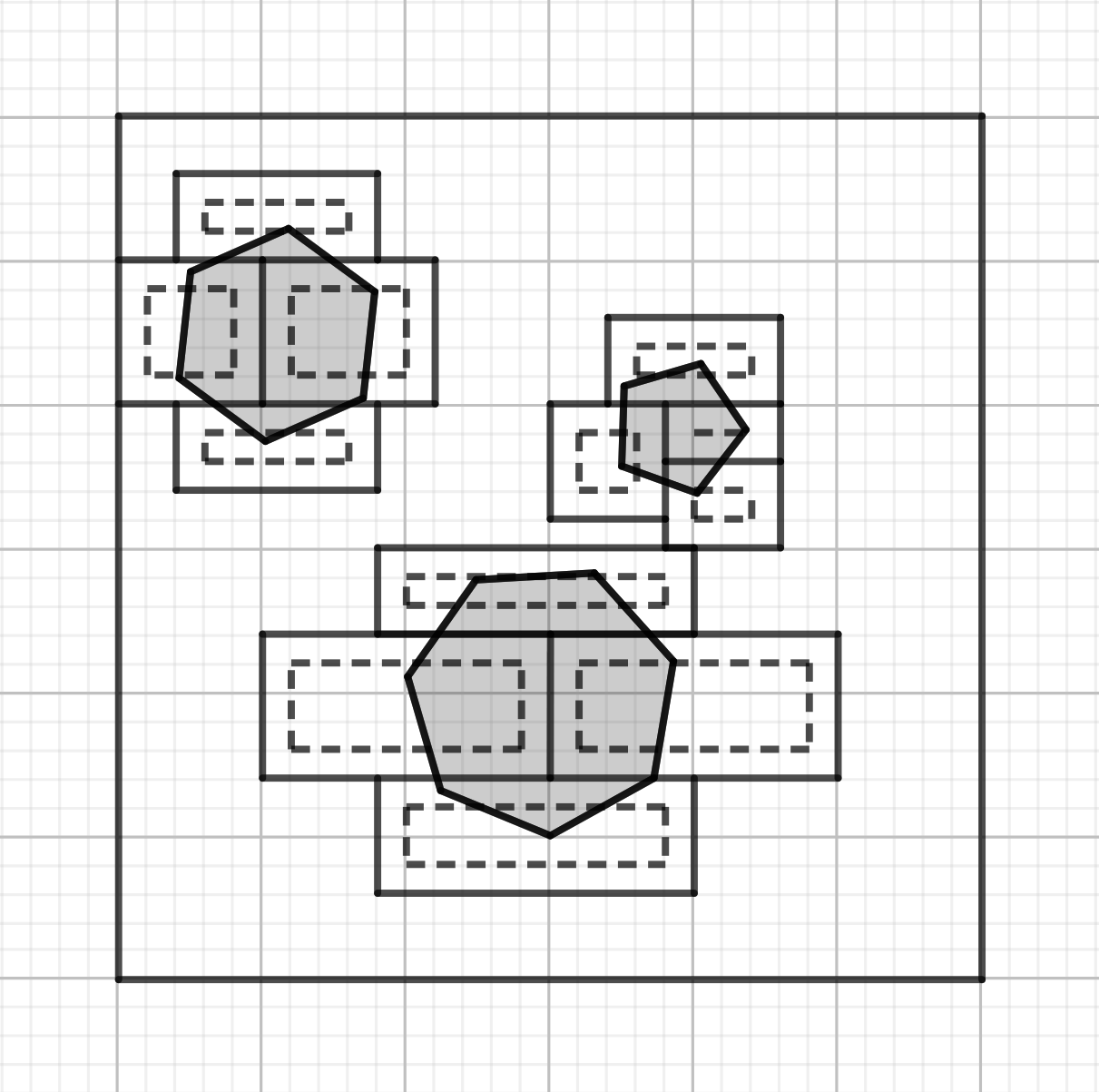
Note that for all by the choice of . Figure 2 shows the collection of sets in the example considered in Figure 1.
Obviously we have . Let
The idea is to construct a neural network for every with which approximates . We obtain the final neural network by parallelizing and adding up these networks. More specifically, we construct a network that approximates the product of and . The latter is approximated by a network which is the concatenation of a network approximating the heaviside function and a network approximating
For , from the prerequisites given in the Theorem we obtain a network with , and weights in with , such that
For technical reasons, we need to slightly change the realisations in order to handle the behaviour of the approximations at the boarder of . Define by its realization
Let . Note that
as well as
Using parallelization and concatenation of Lemma B.1, the function
is a realization of a neural network with at most layers, sparsity
and weights in with . Now let
Note that if . Define as in Lemma B.1 concatenation. The network has layers, sparsity and weights in with for some constants , . Then if and otherwise. Next, for with and , define the network with realization
Note that is a concatenation of two neural networks, since . By Lemma B.2, we can realize the function using a neural network with layers, sparsity and weights in . Thus, has layers, sparsity and weights in . We then define
For we have if and . Otherwise holds. Note that by regarding the construction of , we have for . In order to construct the sum, we used a parallelization of the networks and . Thus, the network has layers, sparsity and weights in with for some constants , 111Note that the notation suggests that the constants differ depending on . However, due to the construction, this is not the case. The superscripts in the notations above are given in order to describe where the constant comes from. For our analysis below, it does not make a difference if the constants change with or not.. Note that Lemma B.2 was used to construct . The realization of the final network is given by
Define . We now verify the desired properties.
We begin by finding constants such that
Clearly, this realization can be achieved with
layers, sparsity
and weights in with
with suitably chosen , . Note that the constants do not depend on .
Next, we show that the set satisfies the desired approximation property . First, for define as follows. Let
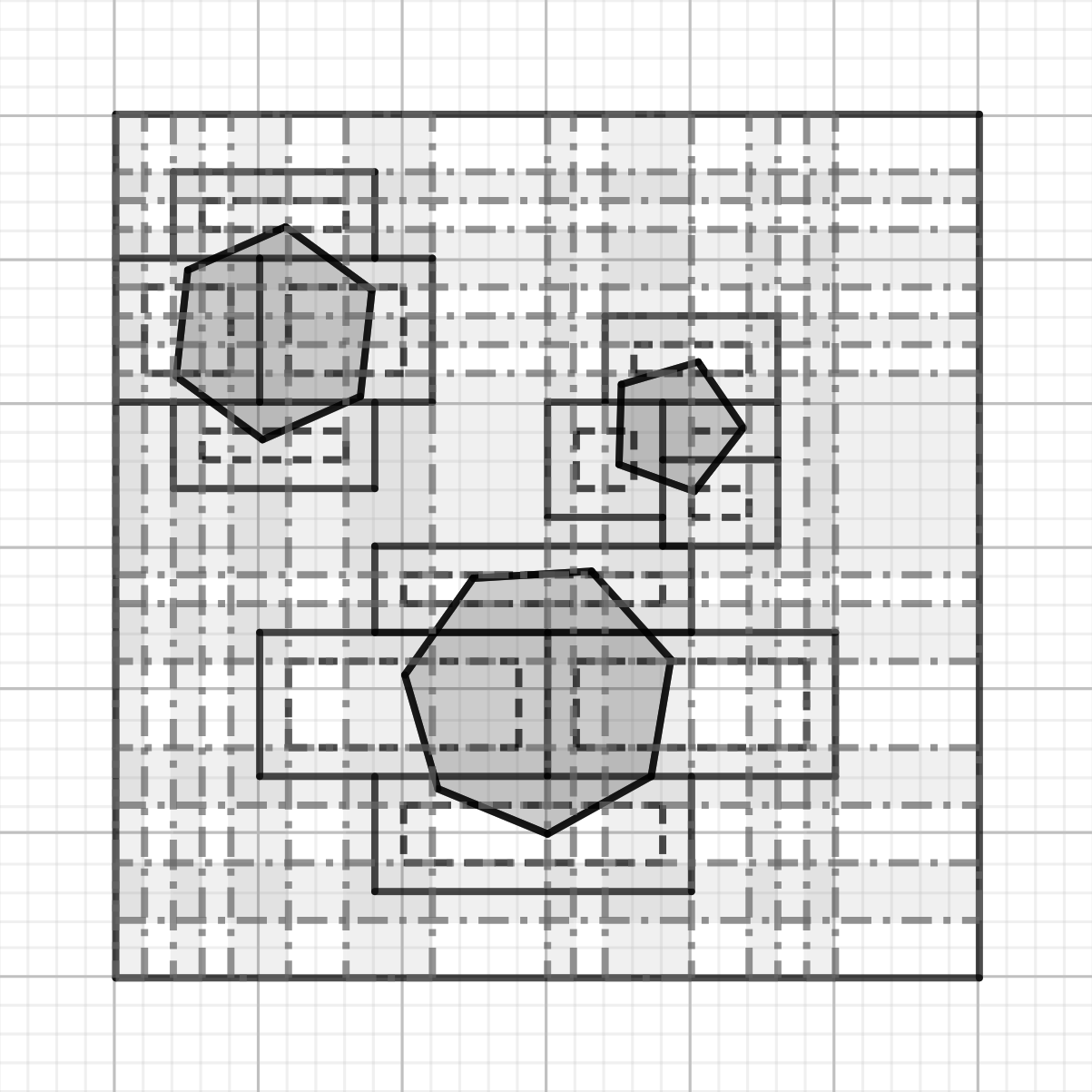
It is easy to see that implies . Set . Figure 3 shows in the example considered in figures 1 and 3.
Clearly . Thus
We need to bound both terms. For we observe that by construction we have
The calculations for the second term are a bit more involved. First, observe that by construction of , for all we have
where
Let be fixed. We have the following cases.
-
•
Assume . Then by construction we have
and thus
-
•
Assume . Then by construction we have
and thus
-
•
Assume , by construction
Consider . Let
Now, for we have
For , by definition of we have
Let and . Using a Taylor expansion, there exists such that
Note that we used the definition of in the last equality for all . Thus
Similarly, for we obtain
This implies
Therefore, we have
for all and which yields
Thus
which concludes the proof. ∎
The remainder of the proof of our main result is now simple.
B.2 Proofs for Regular Boundaries
Next, we prove Lemma 3.6. We first provide the corresponding statement from [21]. Lemma 3.6 is a reformulated version.
Theorem B.4.
(Theorem 5 in [21])
For any function and any integers and there exists a neural network with
layers, sparcity
and weights such that
Proof.
Theorem 5 in [21]. ∎
Proof of Lemma 3.6.
Let be the smallest integer satisfying
where . Let be the smallest integer satisfying
and define . Since and thus we have
Theorem B.4 implies the following. For any there exists a network with
layers, sparsity
and weights such that
Note that
Let be defined as in the proof of Lemma 3.3. Following the proof of Lemma 12 of [21], we see that for any there is a neural network with layers and sparsity such that
where the nonzero weights of are discretized with grid size . Now, define
with
Therefore, all weights are elements of with and
∎
Proof of Lemma 3.9.
Let
with . We first construct a candidate network for . Then, we show that it approximates gamma well and satisfies the required properties.
In order to construct a network that approximates well, we first approximate and using neural networks. The final network is constructed using concatenation and parallelization.
Let , and . Using Lemma 3.6 there exist constants such that there exists a neural network with layers, sparsity and weights in with such that
if . Let . Additionally, the function is the realization of a network with 0 Layers and sparsity .
Since concatenating and parallelizing networks using Lemma B.1 leads to linear transformations on the upper bounds on the Layers, sparsity and the constant , there exist constants , such that the function
with is the realization of a network with
and weights in .
Now, let be small enough. We show that approximates well for suitabily chosen . Following Lemma 9 in [21] we have
for some constant . Set
First, this implies
Additionally, the network has
and weights in for some constants , . ∎
Appendix C Lower Bound
We first prove Theorem 4.1. The outline of the proof is similar to the proof of Theorem 3 in [17]. However, the setting of Theorem 3.5 differs substantially from theirs. This leads to a new situation and new technical challenges to overcome in the proof of Theorem 4.1 .
Proof of Theorem 4.1.
By Hoelders inequality and condition (c) it is enough to consider the case and the first inequality. Let be a finite set of potential probability measures of . Then
Hence, it suffices to show that for any estimator we have
| (C.1) |
for some constant . We now define the set . Then, we prove . Lastly, we show that satisfies (C.1).
Let be an infinitely many times differentiable function with the following properties:
-
•
for ,
-
•
.
Let be an integer. For define
for some small enough. Define
For let
Now, for define as follows. The marginal distribution is the uniform distribution on and
for some . Finally, let
We now show that by properly selecting the constants such that is well defined for all and showing that satisfies the conditions (a),(b),(c).
First of all, we choose small enough and (given ) large enough such that for all we have
for all and .
-
(a)
Clearly, for all the marginal distribution of with respect to has a Lebesgue density which bounded by .
-
(b)
We need to show
for all .
-
1.
Clearly, by selecting , , , and we have
For small enough we also have for all .
-
2.
clear.
-
3.
If , for and we have . Let
Note that for small enough we have . Additionally, we have
-
4.
clear.
This implies the assertion.
-
1.
-
(c)
Let . For we have
For , there is an such that for all we have
Following Proposition 1 in of [22] there exists such that
for all such that . If this implies the assertion with . If not, the assertion is implied by setting .
Next we prove Inequality (C.1). For write for the probability measure of the distribution of when the underlying distribution is . Define the product measure , where is the counting measure on . Note that has a density with respect to which is given by
Assume differ by only 1 entry. We obtain
where for we write with
for . Then, using Assouad’s Lemma we get
We first bound the term . By using the fact that
and Hoelders inequality in the fourth row we calculate
By repeatedly using the fact that , this implies
By independence we have
Additionally, observe that
and
where we used that for all and . Next, we calculate
We need to control the terms and . For the first we obtain
and similarly
This implies
for some constant . By setting we obtain
for some constant for large enough. Thus
for some constant . This concludes the proof. ∎
Lastly, the proof of Theorem 4.2 is provided. The ideas used in the proof are very similar to those used in the proof of Theorem 4.1 above. We therefore only focus on the differences.
Proof of Theorem 4.2.
As in the proof of Theorem 4.1 the strategy is to show that for any estimator we have
for some constant and some finite set . Let be an integer and let
As in the proof of Theorem 4.1 define to be an infinitely many times differentiable function with the following two properties:
-
•
for ,
-
•
.
Note that also fulfills both properties for any , though it may not be infinitely many times differentiable. For define
for and some small enough. Define
For let
Now, for we define as before. The marginal distribution is the uniform distribution on and
for some . Note that for small enough by defining
where
for . The rest of the proof is analogous to the proof of Theorem 4.1. ∎
Acknowledgments
First and foremost, I would like to thank Enno Mammen for supporting me with some helpful comments and inspiring insights during the creation of this paper. Additionally, many thanks goes to Munir Hiabu for assisting with comments during the final stages of the working process.
References
- [1] Jean-Yves Audibert and Alexandre B Tsybakov. Fast learning rates for plug-in classifiers. The Annals of Statistics, 35(2):608–633, 2007.
- [2] Andrew R Barron. Approximation and estimation bounds for artificial neural networks. Machine learning, 14(1):115–133, 1994.
- [3] Thijs Bos and Johannes Schmidt-Hieber. Convergence rates of deep relu networks for multiclass classification. Electronic Journal of Statistics, 16(1):2724–2773, 2022.
- [4] Ronan Collobert and Jason Weston. A unified architecture for natural language processing: Deep neural networks with multitask learning. In Proceedings of the 25th International Conference on Machine Learning, pages 160–167, 2008.
- [5] George Cybenko. Approximation by superpositions of a sigmoidal function. Mathematics of Control, Signals and Systems, 2(4):303–314, 1989.
- [6] Richard M. Dudley. Metric entropy of some classes of sets with differentiable boundaries. Journal of Approximation Theory, 10(3):227–236, 1974.
- [7] Kaiming He, Xiangyu Zhang, Shaoqing Ren, and Jian Sun. Deep residual learning for image recognition. In Proceedings of the IEEE Conference on Computer Vision and Pattern Recognition, pages 770–778, 2016.
- [8] Tianyang Hu, Jun Wang, Wenjia Wang, and Zhenguo Li. Understanding square loss in training overparametrized neural network classifiers. arXiv preprint arXiv:2112.03657, 2021.
- [9] Masaaki Imaizumi and Kenji Fukumizu. Deep neural networks learn non-smooth functions effectively. In The 22nd International Conference on Artificial Intelligence and Statistics, pages 869–878. PMLR, 2019.
- [10] Javed Khan, Jun S Wei, Markus Ringner, Lao H Saal, Marc Ladanyi, Frank Westermann, Frank Berthold, Manfred Schwab, Cristina R Antonescu, Carsten Peterson, et al. Classification and diagnostic prediction of cancers using gene expression profiling and artificial neural networks. Nature Medicine, 7(6):673–679, 2001.
- [11] Yongdai Kim, Ilsang Ohn, and Dongha Kim. Fast convergence rates of deep neural networks for classification. Neural Networks, 138:179–197, 2021.
- [12] Michael Kohler, Adam Krzyżak, and Sophie Langer. Estimation of a function of low local dimensionality by deep neural networks. IEEE Transactions on Information Theory, 2022.
- [13] Michael Kohler and Sophie Langer. Statistical theory for image classification using deep convolutional neural networks with cross-entropy loss. arXiv preprint arXiv:2011.13602, 2020.
- [14] Michael Kohler and Sophie Langer. On the rate of convergence of fully connected deep neural network regression estimates. The Annals of Statistics, 49(4):2231–2249, 2021.
- [15] Yann LeCun, Yoshua Bengio, and Geoffrey Hinton. Deep learning. Nature, 521(7553):436–444, 2015.
- [16] Christian Leibig, Vaneeda Allken, Murat Seçkin Ayhan, Philipp Berens, and Siegfried Wahl. Leveraging uncertainty information from deep neural networks for disease detection. Scientific Reports, 7(1):1–14, 2017.
- [17] Enno Mammen and Alexander B. Tsybakov. Smooth discrimination analysis. The Annals of Statistics, 27(6):1808–1829, 1999.
- [18] Philipp Petersen and Felix Voigtlaender. Optimal approximation of piecewise smooth functions using deep relu neural networks. Neural Networks, 108:296–330, 2018.
- [19] Philipp Petersen and Felix Voigtlaender. Optimal learning of high-dimensional classification problems using deep neural networks. arXiv preprint arXiv:2112.12555, 2021.
- [20] Jürgen Schmidhuber. Deep learning in neural networks: An overview. Neural Networks, 61:85–117, 2015.
- [21] Johannes Schmidt-Hieber et al. Nonparametric regression using deep neural networks with relu activation function. The Annals of Statistics, 48(4):1875–1897, 2020.
- [22] Alexander B. Tsybakov. Optimal aggregation of classifiers in statistical learning. The Annals of Statistics, 32(1):135–166, 2004.
- [23] Qiang Wu and Ding-Xuan Zhou. Svm soft margin classifiers: Linear programming versus quadratic programming. Neural Computation, 17(5):1160–1187, 2005.
- [24] Dmitry Yarotsky. Error bounds for approximations with deep relu networks. Neural Networks, 94:103–114, 2017.