Tracers of Dense Gas in the Outer Galaxy

Abstract

We have mapped HCN and HCO⁺ ($J=1\rightarrow 0$) line emission toward a sample of seven star-forming regions (with $\mathrm{12+log[O/H]}$ range from 8.34 to 8.69) in the outer Milky Way (Galactocentric distance $>9.5$ kpc), using the 14-meter radio telescope of the Taeduk Radio Astronomy Observatory (TRAO). We compare these two molecular lines with other conventional tracers of dense gas, millimeter-wave continuum emission from dust and extinction thresholds ($\mbox{$A_{\rm V}$}\geq 8$ mag), inferred from the ¹³CO line data. HCN and HCO⁺ correlate better with the millimeter emission than with the extinction criterion. A significant amount of luminosity comes from regions below the extinction criterion and outside the millimeter clump for all the clouds. The average fraction of HCN luminosity from within the regions with $\mbox{$A_{\rm V}$}\geq 8$ mag is $0.343\pm 0.225$; for the regions of millimeter emission, it is $0.478\pm 0.149$. Based on a comparison with column density maps from Herschel, HCN and HCO⁺ trace dense gas in high column density regions better than does ¹³CO. HCO⁺ is less concentrated than HCN for outer Galaxy targets, in contrast with the inner Galaxy sample, suggesting that metallicity may affect the interpretation of tracers of dense gas. The conversion factor between the dense gas mass ($M_{\rm dense}$) and line luminosities of HCN and HCO⁺, when integrated over the whole cloud, is comparable with factors used in extragalactic studies.

1 Introduction

Detailed observation of molecular clouds in the Milky Way (Heiderman et al., 2010; Lada et al., 2010, 2012; Evans et al., 2014; Vutisalchavakul et al., 2016) and studies of external galaxies (Gao & Solomon, 2004a) have shown that star formation is more accurately predicted by the amount of dense molecular gas rather than by the total amount of molecular gas. The molecules with high dipole moment and high critical density, such as HCN, HCO⁺ are used as dense gas tracers. The pioneering studies by Gao & Solomon (2004a, b) revealed a tight linear correlation between the luminosity of the HCN $J=1\rightarrow 0$ transition (as a tracer of the mass of dense molecular gas) and the far-infrared luminosity, indicative of the star formation rate (SFR) for whole galaxies. Later works extended this relation to resolved structures in other galaxies (Jiménez-Donaire et al., 2019; Heyer et al., 2022) or even to massive clumps in the Milky Way (Wu et al., 2005; Liu et al., 2016; Stephens et al., 2016; Shimajiri et al., 2017).

Recent studies (Pety et al., 2017; Kauffmann et al., 2017; Evans et al., 2020; Nguyen-Luong et al., 2020) have questioned how well the lowest $J$ transitions of HCN and HCO⁺ trace the dense gas. These authors report that HCN and HCO⁺$J=1\rightarrow 0$ emission is easily detectable from the diffuse part of the cloud with typical density $\mathrm{100-500\ cm^{-3}}$. The concept of detecting a particular line above or around the critical density ($n_{c}$) is oversimplified (Evans, 1989). In reality, multilevel excitation effects and radiative trapping effects all tend to lower the effective excitation density ($n_{eff}$), defined as the density needed to detect a molecular line with integrated intensity of 1 K km s^-1 (Evans, 1999; Shirley, 2015). For the low-$J$ transitions the effective excitation densities are typically 1-2 orders of magnitude lower than the critical densities. The values of $n_{eff}$ for HCN and HCO⁺ are $4.5\times 10^{3}\ \mathrm{cm^{-3}}$ and $5.3\times 10^{2}\ \mathrm{cm^{-3}}$ at 20 K, respectively (Shirley, 2015). For modern surveys with low RMS noise, lines at the detection limits can be produced by gas with density as low as 50-100 cm^-3, explaining the emission from extended translucent regions where the density of gas is much lower than the critical densities of HCN, HCO⁺ (Evans et al., 2020).

Pety et al. (2017) found that only a small fraction of the luminosity of HCN(18%) and HCO⁺(16%) arises from regions with $\mbox{$A_{\rm V}$}>15$ mag for Orion B. Kauffmann et al. (2017) found that HCN($J=1\rightarrow 0$) mainly traces gas with $\mbox{$A_{\rm V}$}\approx 6$ mag, or $n\approx 870\ \mathrm{cm^{-3}}$ towards Orion A. A substantial fraction (44-100%) of the total line luminosities of HCN and HCO⁺arises outside the $\mbox{$A_{\rm V}$}>8$ mag region often associated with star formation for 6 inner Galaxy clouds (Evans et al., 2020). Most dense cores and YSOs are found at $\mbox{$A_{\rm V}$}\geq 8$ mag (Heiderman et al., 2010; Lada et al., 2010, 2012).

None of the studies described above considered the star forming regions in the outer Galaxy, i.e., clusters having Galactocentric  distance ($R_{G}$) greater than $\sim 8.2$ kpc. The star-forming regions in the outer Galaxy (low-density regime) behave distinctively from the environment around the solar neighborhood (intermediate density regime) and also from the Central Molecular Zone (CMZ, high-density regime) (Kennicutt & Evans, 2012). The physical and chemical conditions in star-forming regions are dependent on the environment, which is in turn a function of Galactocentric radius ($R_{G}$).

The Milky Way and other normal spiral galaxies are known to have a negative gradient of metallicity with $R_{G}$ (Searle, 1971). Many studies have found a radial abundance gradient of oxygen, nitrogen, etc. in the Milky Way (Deharveng et al., 2000; Esteban et al., 2017; Esteban & García-Rojas, 2018). Most recently, Méndez-Delgado et al. (2022) report linear radial abundance gradients for $\mathrm{O/H}$, $\mathrm{N/H}$ with slopes of $-0.044\pm 0.009\ \rm dex\ kpc^{-1}$, $-0.063\pm 0.009\ \rm dex\ kpc^{-1}$, respectively, for $R_{G}=$ 4.88 to 17 kpc and for $\mathrm{C/H}$ the slope is $-0.077\pm 0.019\ \rm dex\ kpc^{-1}$ for $R_{G}=6.46$ to $11.6$ kpc. The efficiency of gas cooling and dust shielding processes decrease at lower metallicity, thereby affecting the condensation and fragmentation of giant molecular clouds (GMCs). Conversely, the lower interstellar radiation field and cosmic-ray fluxes at larger $R_{G}$ decreases the gas heating (Balser et al., 2011). The balance between these processes sets the gas and dust physical conditions may cause different star formation outcomes from those in the CMZ or Solar neighborhood. While studies of nearby galaxies (LMC, SMC) with low metallicity are used to understand these effects (Galametz et al., 2020), the outer Milky Way is much closer to us. The outer Galaxy targets provide a less confusing view of the ISM as they are widely separated and there is no blending of emission. This clear perspective of the outer Galaxy enables studies of individual giant molecular clouds from which global properties of star formation can be estimated. Thus, studying the star forming regions in the outer Galaxy can bridge the gap between the star formation studies in Galactic and extragalactic environments.

To inform interpretation of extragalactic studies, we investigate the distribution of HCN and HCO⁺ $J=1\rightarrow 0$ emission over the full area of molecular clouds and range of physical conditions. This work complements the inner Galaxy work (Evans et al., 2020) for the outer Galaxy.

2 Sample

We selected 7 targets beyond the solar circle with $\mbox{$R_{G}$}>9.5\ \mbox{kpc}$ with diversity in properties such as cloud mass, physical size, number of massive stars, metallicity etc (see Table 1). We also considered the availability of molecular data (¹²CO and ¹³CO emission from the Extended Outer Galaxy survey, see 3.2), dust emission from the BGPS survey (Ginsburg et al., 2013) and FIR emission from Herschel data (Marsh et al., 2017). Several distance values are available in the literature based on kinematic or stellar measurements. In order to maintain uniformity we adopt the GAIA EDR3 based distance values of all the targets (except S252) from Méndez-Delgado et al. (2022) and use the same methodology to obtain the distance for S252. The distance of the Sun from the Galactic Center is taken as 8.2 kpc (Gravity Collaboration et al., 2019). $R_{G}$ values of our sample range between 9.85 to 14.76 kpc (see Table 1).

The spectral type(s) (SpT) of the main ionizing star(s) and 12+log[O/H] values of each target and their respective references are also given in Table 1. We mapped the HCN and HCO⁺ ($J=1\rightarrow 0$) emission from the parent clouds of 7 H II regions over an area based on ¹³CO emission (see details in Section 3). The cloud mass ($M_{\rm cloud}$) is obtained using the CO data described in §3 and $\mbox{$M_{\rm cloud}$}=\alpha_{\mathrm{CO}}L_{\mathrm{CO}}$ with $\alpha_{\mathrm{CO}}=4.3\ \mathrm{M_{\odot}\ (K\ km\ s^{-1}pc^{2})^{-1}}$, where $L_{\mathrm{CO}}$ is the luminosity expressed in $\mathrm{K\ km\ s^{-1}pc^{2}}$ (Bolatto et al., 2013). A brief description of each region can be found in §Appendix A.

3 Observations and Data Sets

3.1 HCN and HCO⁺ Observations with TRAO

We mapped the seven outer Galaxy clouds in the HCN ($J=1\rightarrow 0$, 88.631847 GHz) and HCO⁺($J=1\rightarrow 0$, 89.1885296 GHz) lines simultaneously at Taeduk Radio Astronomy Observatory (TRAO) in January 2020. The TRAO telescope is equipped with the SEcond QUabbin Optical Image Array (SEQUOIA-TRAO), a multi-beam receiver with 16 pixels in a $4\times 4$ array and operates in 85-115 GHz range. The back-end has a 2G FFT (Fast Fourier Transform) Spectrometer. The instrumental properties are described in Jeong et al. (2019). The TRAO has a main-beam size of 58″ at these frequencies and a main-beam efficiency (defined so that $T_{\rm mb}=T_{A}^{*}/(f_{b}\eta_{\rm mb})$, where $T_{\rm mb}$ is the Rayleigh-Jeans main-beam temperature and $f_{b}$ is the fraction of the beam filled by the source) of 46% at 89 GHz (Jeong et al., 2019). The individual SEQUOIA beams vary in beam size (efficiency) by only a few arcseconds (few percent). The beams are very circular and beam efficiencies vary less than $3\%$ with elevation angle.

We used the OTF (On-The-Fly) mode to map the clouds. The mapped areas for the individual targets were determined from maps of their ¹³CO ($J=1\rightarrow 0$) line emission. We used a threshold value of 5 times the RMS noise in the ¹³CO map to estimate the mapping area for HCN and HCO⁺  from the TRAO 14-m telescope. The $A_{\rm V}$ values corresponding to the threshold values are listed in Table 1. All the targets were mapped in Galactic co-ordinates. The mapped areas for individual targets are listed in Table 1.

The system temperature was $\sim 190\rm K$ during HCN and HCO⁺ observations. We used $\rm SiO$ maser sources at 86 GHz for pointing and focusing the telescope every 3 hours. We smoothed the data with the boxcar function to a velocity resolution of about 0.2 km s^-1, resulting in an RMS sensitivity of 0.06-0.08 K on the $T_{A}^{*}$ scale for all the targets. We obtained $\sim 150\ \rm hrs$ of observations in total.

The following steps were done to reduce the data. We used the OTFTOOL to read the raw on-the-fly data for each map of each tile and then converted them into the CLASS format map after subtracting a first order baseline. We applied noise weighting and chose the output cell size of $20\arcsec$ in OTFTOOL. We did not apply any convolution function to make the maps, so the effective beam size is same as the main-beam size. Further reduction was done in CLASS format of GILDAS, where we chose the velocity range ($v_{sp}$) to get good baselines on each side of the velocity range of significant emission ($v_{win}$). The reduction details are listed in §Appendix B Table LABEL:tab:reduction. We subtracted a second-order polynomial baseline and converted those files to FITS format using GREG.

3.2 Ancillary data available

For this work, we have also used the following data sets :

1. ¹²CO and ¹³CO ($J=1\rightarrow 0$) Observations: ¹²CO and ¹³CO data for all the targets are extracted from the Exeter-FCRAO, Extended Outer Galaxy survey using the Five College Radio Astronomy Observatory (FCRAO) 14-m telescope. The EXFC survey covered ¹²CO and ¹³CO $J=1\rightarrow 0$ emission within two longitude ranges: $55^{\circ}<l<100^{\circ}$ with the Galactic Latitude range $-1.4^{\circ}\leq b\leq+1.9^{\circ}$ and $135^{\circ}<l<195^{\circ}$ with Galactic Latitude range $-3.6^{\circ}<b<5.6^{\circ}$ (Roman-Duval et al., 2016). Our outer Galaxy targets are covered by the latter survey. The angular resolution of ¹²CO and ¹³CO are $45\arcsec$ and $48\arcsec$ respectively and the grid size is $22.5\arcsec$. The spectral resolution is 0.127 km s^-1. All of the data have been de-convolved to remove contributions from the antenna error beam and therefore, are in main beam temperature units.

2. Millimeter Dust Continuum Emission: We use 1.1 mm continuum emission data from the Bolocam Galactic Plane Survey (BGPS) using Bolocam on the Caltech Submillimeter Observatory. The BGPS Survey does not cover the outer Galaxy regions uniformly; it covers four targeted regions (IC1396, a region towards the Perseus arm, W3/4/5 and Gem OB1). The effective resolution of this survey is $33\arcsec$. We use the mask files of the sources from V2.1 table, where the pixel values in the mask file are set with the catalog number where the source is above the $2\sigma$ threshold; otherwise the pixel values are zero (Ginsburg et al., 2013). The Bolocat V2.1 contains the 1.1 mm photometric flux of 8594 sources for the aperture radii of $20\arcsec$, $40\arcsec$, and $60\arcsec$ and it also provides flux densities integrated over the source area. As this is not a contiguous survey towards the outer Galaxy, not all the targets have BGPS data. The data availability of the targets are indicated by the footnotes in Table 1.

3. Far-Infrared data: We have used the column density maps determined from Herschel data (Marsh et al., 2017) and available at the Herschel infrared Galactic Plane (Hi-GAL) survey site table. These column density maps are derived using the PPMAP procedure (Marsh et al., 2015) on the continuum data in the wavelength range 70-500 $\rm\mu$m from the Hi-GAL survey. The spatial resolution of the maps is $12\arcsec$. Not all the targets in our list are covered by the Hi-GAL survey. Table 1 shows the data availability.

4 Results and Analysis

Our goal is to compare the luminosities of HCN and HCO⁺ $J=1\rightarrow 0$ transitions to other conventional tracers of dense gas, in particular extinction thresholds and millimeter-wave emission from dust. We estimate the extinction from the ¹³CO data and relations between gas column density and extinction. For the emission from dust, we use the mask file of the BGPS data, an indicator of the existence of gas of relatively high volume density (Dunham et al., 2011). We also examine the ability of HCN, HCO⁺, and ¹³CO to trace column density, determined from Herschel maps.

4.1 Luminosity calculation based on Extinction criterion

This section describes the method of calculating luminosity of the line tracers coming from the dense regions and also from outside the dense region, depending on ¹³CO column density based extinction($A_{\rm V}$) map. It consists of two main steps: (i) making molecular hydrogen column density ($\rm N(H_{2})$) maps of each target, convertible into maps of $A_{\rm V}$; and (ii) measuring the luminosity of regions satisfying the $A_{\rm V}$ criterion.

4.1.1 Identifying the pixels with $\mbox{$A_{\rm V}$}\geq 8$ mag

To derive the molecular hydrogen column density maps of each target, we use their ¹²CO and ¹³CO data. We first identify the velocity range by examining the spectrum of ¹³CO emission averaged over the whole mapped region of each target. The method of making column density maps of ¹³CO is discussed in detail in §Appendix C. We follow equation C1-C5 from §Appendix C to produce the total column density map of ¹³CO (N(¹³CO)) using ¹³CO and ¹²CO data. Next, we convolve and regrid the ¹³CO column density map to match the TRAO map and convert it to a molecular hydrogen column density map using the following equation.

$$\rm{N(H_{2})}=\rm{N(\mbox{${}^{13}$CO})}\left[\frac{\rm{H_{2}}}{\rm{CO}}\right]\left[\frac{\rm{CO}}{\mbox{${}^{13}$CO}}\right]$$ (1)

We assume a fractional abundance of 6000 for CO (Lacy et al., 2017) and we apply the $[^{12}$C]/[¹³C] isotopic ratio recently derived by Jacob et al. (2020). This ratio is linearly dependent on the Galactocentric  distance ($R_{G}$) of the target.

$$\frac{[^{12}\mbox{C}]}{[^{13}\mbox{C}]}=5.87\times\frac{\mbox{$R_{G}$}}{\mathrm{kpc}}+13.25$$ (2)

Finally, we use the relation $\mbox{$A_{\rm V}$}=1.0\times 10^{-21}\mbox{$\rm N(H_{2})$}$ to convert the molecular hydrogen column density to extinction (Lacy et al., 2017). This procedure allows us to define the pixels satisfying the criterion: $\mbox{$A_{\rm V}$}\geq 8$ mag.

4.1.2 The Emission from the Total region and Inside Region with $\mbox{$A_{\rm V}$}\geq 8$ mag

Next we calculate the average spectrum for two regions: (1) including all pixels in the dense region and (2) all pixels outside the dense region based on the $A_{\rm V}$ criterion ($1.5\leq\mbox{$A_{\rm V}$}<8$ mag). The lower limit on $A_{\rm V}$ is based on 5 times the RMS noise threshold in the ¹³CO maps. Because the RMS noise levels are not the same for all the clouds (see Table 1), we use $\mbox{$A_{\rm V}$}=1.5$ mag as the lower limit to make the analysis uniform.

We first identify the dense regions with $\mbox{$A_{\rm V}$}\geq 8\ \rm{mag}$ in the extinction map (denoted by in). Figure 1 shows the integrated intensity map of HCN and HCO⁺ for all the targets; white contours on each image in Figure 1 indicate the $\mbox{$A_{\rm V}$}\geq 8$ mag regions. The spectra averaged over pixels that satisfy the criterion $\mbox{$A_{\rm V}$}\geq 8\ \rm{mag}$ (blue line) and the spectra for pixels that do not (denoted out and shown in red line) are shown in Figure 2 (a, b and upper panels of c, d, e, f, g). Figure (2c) (S212) does not show any blue line in the upper panel because there is no pixel satisfying the $\mbox{$A_{\rm V}$}\geq 8\ \rm{mag}$ criterion. The average spectral lines from the in region are stronger than those from the out region whenever both spectra are available. One odd feature appears in Figure 1 (S228): the HCN and HCO⁺ agree well with the BGPS, but there is no peak in $A_{\rm V}$ in that region. Figure (2d) does not show strong emission for HCN and HCO⁺ at the position of $\mbox{$A_{\rm V}$}\geq 8$ mag region (upper panel). This oddity and other information regarding individual targets are described in §Appendix A.

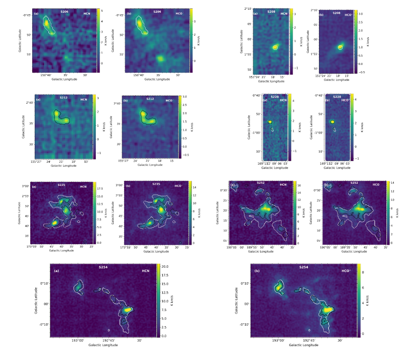
Figure 1: This figure shows the integrated intensity map of (a) HCN and (b) HCO⁺ for each target (name of each targets are mentioned in each image). The white contours indicate the $\mbox{$A_{\rm V}$}\geq 8$ mag regions and black contours indicate the BGPS mask regions. There are no black contours in S206 and S208 as they lack BGPS data. There is no white contour in S212, as there is no region above $\mbox{$A_{\rm V}$}=8$ mag.

Figure 2: This is the average spectrum plot for the cloud (a)S206, (b)S208, (c)S212, (d)S228, (e)S235, (f)S252 and (g)S254 based on $A_{\rm V}$ criterion and BGPS mask map. The left panel in all images are for HCN and right panels are for HCO⁺. The blue line indicates the line emission coming from $\mbox{$A_{\rm V}$}\geq 8$ mag regions and red line indicates the emission from $1.5\leq\mbox{$A_{\rm V}$}<8$ mag regions in top panel of each sub-figure. In the bottom panels of each sub-figures (except (a) and (b)), the blue line indicates emission coming from the BGPS masked region and red line is for emission outside the masked region.

For the calculation of luminosity, we use the main-beam corrected temperature of species $X$ ($T_{X}=T_{A}^{*}/\eta_{mb}$, where $\eta_{mb}=0.46$). The velocity ranges for ¹³CO and HCO⁺ are similar and for HCN we expand the velocity range to account for the hyperfine structure (around 3-6 km s^-1 on each side depending on the target requirements). The velocity ranges are explained in §Appendix B.

We measure the luminosity of species $X$ arising from the $\mbox{$A_{\rm V}$}\geq 8\ \rm{mag}$ region using the following equation:

$$L_{\rm X,in}=D^{2}\int_{v_{\rm sp,l}}^{v_{\rm sp,u}}dv\int d\Omega_{in}T_{X}(l,b,v),$$ (3)

where $D$ is the distance of the target from the Sun in pc and the integrals are taken over the line velocity between $v_{\rm sp,l}$ and $v_{\rm sp,u}$, the lower and upper limits of the line spectral window, and the solid angle that satisfies the extinction criterion. In practice, we use the average spectrum in Figure 2 to define the integrated intensity

$$I_{\rm X}=\int_{v_{\rm sp,l}}^{v_{\rm sp,u}}T_{X}dv$$ (4)

and compute the luminosity from the following equation:

$$L_{\rm X,in}=D^{2}{I_{\rm X}}N_{\rm in}\Omega_{\rm pix},$$ (5)

where $N_{\rm in}$ is the number of pixels satisfying the in condition and $\Omega_{\rm pix}$ is the solid angle of a pixel.

The uncertainty in luminosity is

$$\sigma_{L}=D^{2}\delta v\sqrt{N_{ch}}\ \sigma_{T_{X}}\ N_{\rm in}\Omega_{\rm pix},$$ (6)

where $N_{ch}$ is the number of channels in the line region, $\delta v$ is the channel width, and $\sigma_{T_{X}}$ is the RMS noise in the baseline of the average spectrum.

To calculate the total luminosity ($L_{\rm X,tot}$), we follow the same method but include all pixels with $\mbox{$A_{\rm V}$}>1.5\ \rm mag$ for $L_{\rm X,tot}$.

We follow the same procedure for HCN, HCO⁺ and ¹³CO; for ¹³CO, we made integrated intensity maps for the specified velocity range using the FITS files from FCRAO and these maps are convolved, resampled, and aligned with the TRAO maps.

We tabulated the values for the fraction of pixels inside the $A_{\rm V}$ criterion ($N_{\rm in}/N_{\rm tot}$), the log of total line luminosity (Log $L_{\rm tot}$), the log of the line luminosity coming from the $\mbox{$A_{\rm V}$}\geq 8\ \rm mag$ region (Log $L_{\rm in}$) and the fractional luminosity ($f_{\rm L}$$=L_{in}/L_{tot}$) in Table 2 for HCN, HCO⁺and ¹³CO. Also we have given the statistical parameters (mean, standard deviation and median) for the relevant columns. S212 has no pixels with $\mbox{$A_{\rm V}$}\geq 8\ \rm mag$.

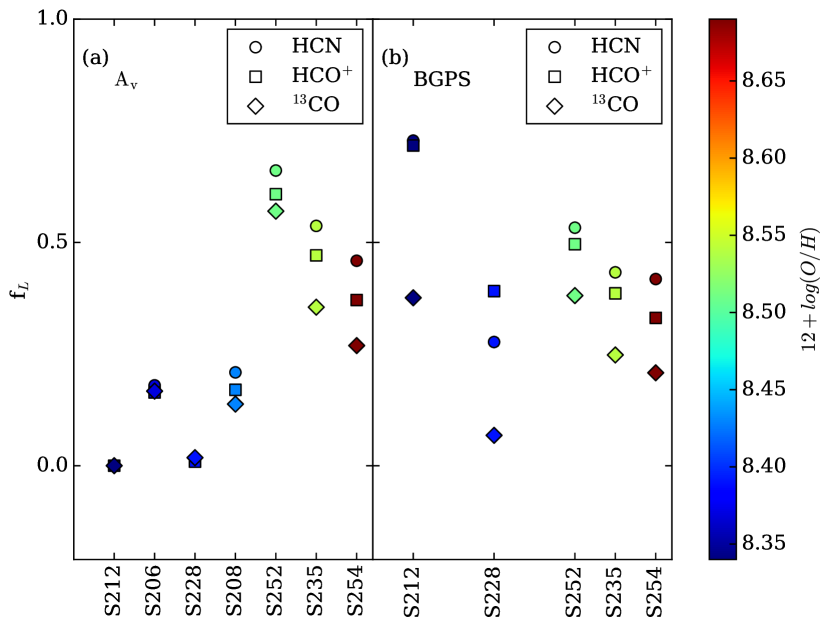
Figure 3: The fraction of luminosity ($f_{\rm L}$) within in region is plotted for each tracer versus clouds. The $f_{\rm L}$ in the left panel is obtained from $\mbox{$A_{\rm V}$}\geq 8$ mag region and in the right panel, $f_{\rm L}$ is from BGPS mask region. The targets are organized with increasing metallicity. Different symbols are used to separate the different tracers. Different color indicates the metallicity of each source.

Figure 3a shows $f_{\rm L}$ within the in regions defined by $\mbox{$A_{\rm V}$}\geq 8$ mag (left) for each cloud sorted by increasing metallicity. The values of $f_{\rm L}$ vary between 0.014 and 0.661 for HCN, between 0.009 and 0.608 for HCO⁺, and between 0.018 and 0.570 for ¹³CO. The values of $f_{\rm L}$ for HCN are higher than HCO⁺ and ¹³CO. The mean value of the line luminosities coming from the in region is higher by 0.12 for HCN compared to HCO⁺. For ¹³CO, $L_{\rm in}$ is higher but the values of fractional luminosity ($f_{\rm L}$) are lower than those of HCN and HCO⁺. In terms of the logarithm of the total line luminosity, the mean is 2.78 for ¹³CO, 1.98 for HCO⁺ and 1.99 for HCN. Comparing the two dense gas tracers, HCO⁺ and HCN provide similar total luminosity, but HCN shows better correlation with the extinction criterion in terms of $f_{\rm L}$ followed by HCO⁺ and ¹³CO (see Figure 3a).

The correlation between fractional line luminosity ($f_{\rm L}$) arising from the $\mbox{$A_{\rm V}$}\geq 8$ mag region with Log  $L_{\rm tot}$ and Log  $L_{\rm in}$ (Figure 4) shows that the clouds with more material (i.e., higher luminosity) tend to have higher values of $f_{\rm L}$.

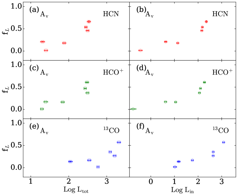
Figure 4: The fraction of line luminosity arising above $\mbox{$A_{\rm V}$}\geq 8$ mag is plotted versus line luminosity. HCN is plotted on the top, HCO⁺on the middle, and ¹³CO on the bottom. The total line luminosities ($\mathrm{LogL_{tot}}$) are on the left and luminosity from in region ($\mathrm{LogL_{in}}$) on right

4.2 Luminosity calculation from BGPS

In this section, we follow the same basic method but use the dust thermal continuum emission to trace the ‘dense’ gas. We use the data from BGPS to compare the line tracers in those regions. Millimeter continuum dust emission remains an optically thin tracer of the gas column density even in dense molecular clouds and efficiently identifies the molecular clumps that are possible sites of star formation. Because of the limits on sensitivity to large angular scale emission, the BGPS emission traces volume density, but the characteristic density probed decreases with distance (Dunham et al., 2011). For distances in this sample of 2-6 kpc, the mean density traced is 5${}\times 10^{3}$ to 1${}\times 10^{4}$ cm^-3 (Fig. 12 of Dunham et al. 2011) with properties of clumps rather than cores or clouds. We use the mask maps of BGPS, downloaded from Bolocat V2.1 to define the in region. As before, we then computed the line luminosities inside and outside the mask regions.

First, we changed the BGPS mask maps to the same resolution and pixel size as the TRAO maps. Next we make the average spectra of the in and out regions and use equation 5 to calculate the luminosity for HCN, HCO⁺ and ¹³CO. The total luminosities ($L_{\rm tot}$) are the same as those obtained using the extinction condition $\mbox{$A_{\rm V}$}\geq 8\ \rm mag$ in Section 4.1.

Among all the targets, 5 of the regions are covered by the BGPS survey. The black contours on the integrated intensity maps of HCN and HCO⁺ in Figure 1 show the position of the BGPS in region. The bottom panels of Figure 2(c, d, e, f, g) show the average spectra of the luminosities coming from the BGPS in and out regions. All 5 targets show clear detection of HCN and HCO⁺ from the BGPS mask region, but significant emission is coming from outside the BGPS mask regions.

We present the result of those five targets in Table 3 along with the mean, standard deviation and median for relevant columns. We have listed the values for the fraction of pixels inside the BGPS mask region ($N_{\rm{in}}/N_{\rm{tot}}$), the log of the total line luminosity (Log $L_{\rm tot}$), the log of line luminosity arising from the BGPS in region (Log $L_{\rm in}$) and the fractional luminosity ($f_{\rm L}$$=L_{in}/L_{tot}$) in Table 3 for HCN, HCO⁺and ¹³CO.

The mean $f_{\rm L}$ values, listed in Table 3, are higher for HCN, followed by HCO⁺ and ¹³CO (see Figure 3b). Dense line tracers (HCN, HCO⁺) show better agreement with BGPS emission than they did with the extinction criterion ($\mbox{$A_{\rm V}$}\geq 8\mathrm{mag}$) for these 5 clouds having BGPS data.

The standard deviation of the $f_{\rm L}$ values is 0.149 and 0.137 for HCN and HCO⁺ respectively, considerably lower than the values for the extinction criterion. Figure 5 shows the correlation between fractional line luminosity ($f_{\rm L}$) arising from inside the BGPS mask region with Log$L_{\rm in}$ and total luminosity Log$L_{\rm tot}$. The $f_{\rm L}$ values show no significant dependence on Log  $L_{\rm tot}$ and Log  $L_{\rm in}$ for any of the 3 tracers.

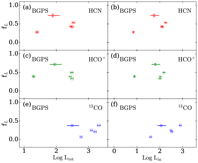
Figure 5: The fraction of line luminosity arising from the BGPS mask region is plotted versus line luminosity. HCN is plotted on the top, HCO⁺on the middle, and ¹³CO on the bottom. The total line luminosities ($\mathrm{LogL_{tot}}$) are on the left and luminosity from in region ($\mathrm{LogL_{in}}$) on right.

4.3 Conversion of Line Luminosity to Mass of Dense Gas

In this section, we measure the mass conversion factor for the outer Galaxy targets. The conversion factor is defined as the ratio between the mass of gas and line luminosities ($M=\alpha_{Q}L_{Q}$, where the unit of $\alpha_{Q}$ is $\mathrm{\mbox{M${}_{\odot}$}(K\ km\ s^{-1}\ pc^{2})^{-1}}$. This conversion factor is used in extragalactic studies to estimate the mass of dense gas.

The dense gas mass of each source having BGPS data is estimated from its integrated flux density, $S_{1.1}$ (available in BGPS Source catalog table, Rosolowsky et al. 2010) combined with distance ($D$) and dust temperature ($T_{dust}$). The 1.1 mm dust emission is assumed to be optically thin and at a single temperature, and a dust opacity is assumed.

$$\mbox{$M_{\rm dense}$}=\frac{S_{1.1}D^{2}(\rho_{g}/\rho_{d})}{B_{\nu}(T_{dust})\kappa_{dust,1.1}}$$ (7)

where $B_{\nu}$ is the Planck function evaluated at $\lambda=1.1$ mm, $\kappa_{dust,1.1}=1.14$ $\rm{cm^{2}g^{-1}}$ is the dust opacity per gram of dust (Enoch et al., 2006) and gas-to-dust ratio ($\rho_{g}/\rho_{d}$) is assumed to be 100 (Hildebrand, 1983). We use the relation after scaling it (Rosolowsky et al., 2010)

$$\mbox{$M_{\rm dense}$}=13.1M_{\odot}\left(\frac{D}{1\mathrm{kpc}}\right)^{2}\left(\frac{S_{1.1}}{1\mathrm{Jy}}\right)\left[\frac{e^{(13.0\mathrm{K}/T_{dust})}-1}{e^{(13.0/20)}-1}\right]$$ (8)

For consistency with Rosolowsky et al. (2010), we assume a single dust temperature ($T_{dust}=20$ K) for all sources to estimate the dense gas mass. For the sources with Herschel data, the derived $T_{dust}$ is consistent with this choice. The values of dense mass ($M_{\rm dense}$) are listed in Table 4 in logarithmic scale. The uncertainties include distance uncertainties.

The mass conversion factor $\alpha_{\rm tot}$ is calculated as the mass of dense gas divided by the total luminosity of the clouds ($\mbox{$A_{\rm V}$}>1.5$ mag) ($\mbox{$\alpha_{\rm tot}$}=\mbox{$M_{\rm dense}$}/\mbox{$L_{\rm tot}$}$) and for $\alpha_{\rm in}$ the luminosity is restricted to the dense region based on BGPS mask ($\mbox{$\alpha_{\rm in}$}=\mbox{$M_{\rm dense}$}/\mbox{$L_{\rm in}$}$). In Table 4, we list the conversion factors along with total line luminosities ($L_{\rm tot}$), line luminosities inside the BGPS mask ($L_{\rm in}$) in logarithmic scale for HCN and HCO⁺. We also estimated the statistical parameters (mean, standard deviation and median) to understand the correlation between $M_{\rm dense}$ and the conversion factors ($\alpha_{\rm in}$, $\alpha_{\rm tot}$). The mean value of $\alpha_{\rm in}$ in logarithmic scale is $\langle\mathrm{Log\ \mbox{$\alpha_{\rm in}$}(\mbox{{\rm HCN}})}\rangle=1.28\pm 0.08$, translating to $\mbox{$M_{\rm dense}$}=19^{+3.8}_{-3.2}\mbox{$L_{\rm in}$}(\mbox{{\rm HCN}})$ and for $\alpha_{\rm tot}$, $\langle\mathrm{Log\ \mbox{$\alpha_{\rm tot}$}(\mbox{{\rm HCN}})}\rangle=0.93\pm 0.16$, translating to $\mbox{$M_{\rm dense}$}=8.5^{+3.8}_{-2.6}\mbox{$L_{\rm tot}$}(\mbox{{\rm HCN}})$. Our $\alpha_{\rm tot}$ value is close to the extragalactic conversion factor ($\alpha_{\rm{HCN(1-0)}}=10$ M_⊙$\mathrm{(K\ km\ s^{-1}\ pc^{2})^{-1}}$, Gao & Solomon (2004b)), where luminosity from the whole cloud is considered to obtain mass. The $\alpha_{\rm in}$ value is similar to the value obtained by Wu et al. (2010) for dense clumps. The theoretical prediction of $\mathrm{\alpha(HCN)}$ by Onus et al. (2018) is $14\pm 6$ $\mathrm{\mbox{M${}_{\odot}$}(K\ km\ s^{-1}\ pc^{2})^{-1}}$ for $n\geq$1${}\times 10^{4}$ cm^-3 which corresponds to the dense gas of the cloud. Including the uncertainty, this theoretical value is consistent with either our $\alpha_{\rm in}$(HCN) or $\alpha_{\rm tot}$(HCN). Calculations for HCO⁺ yields $\mathrm{\mbox{$\alpha_{\rm in}$}=20.4^{+4.1}_{-3.4}}$ $\mathrm{\mbox{M${}_{\odot}$}(K\ km\ s^{-1}\ pc^{2})^{-1}}$ and $\mathrm{\mbox{$\alpha_{\rm tot}$}=9.1^{+3.2}_{-2.3}}$ M_⊙$\mathrm{(K\ km\ s^{-1}\ pc^{2})^{-1}}$, similar to the values for HCN.

Variation in $T_{dust}$ by $\pm 3$ K produce changes in $\alpha_{\rm in}$ and $\alpha_{\rm tot}$ within the variation among sources, whereas variation by $5$ K in dust temperature begin to produce changes outside that range. Higher $T_{dust}$ of course produce lower values of $\alpha_{\rm in}$, $\alpha_{\rm tot}$; lower $T_{dust}$ gives higher values.

We also estimate the mass of BGPS clumps from the Herschel based column density maps from Marsh et al. (2017) for S228, S252 and S254. We use $\mathrm{M_{dense}=\mu_{H_{2}}m_{H}A_{pix}\sum N(H_{2})}$, where mean molecular weight $\mathrm{\mu_{H_{2}}}$ is assumed to be 2.8 (Kauffmann et al., 2008), $\mathrm{m_{H}}$ is mass of hydrogen, $\mathrm{A_{pix}}$ is area of a pixel in $\mathrm{cm^{2}}$ and $\mathrm{\sum N(H_{2})}$ is the integrated column density. The mass values in logarithmic scale are 2.36, 4.09 and 3.72 respectively for 3 targets. The values are higher than BGPS mass measurement by average 0.34 in log scale, which is 2.2 in linear scale. The difference in the values is mainly caused by differing assumptions about the dust opacity. Marsh et al. (2017) used $\mathrm{\kappa(\lambda)=0.1(\frac{\lambda}{300})^{-2}}$ $\mathrm{cm^{2}g^{-1}}$, which implies a dust opacity per gram of dust at 1.1 mm of $\mathrm{\kappa_{1.1}}=0.74$ $\mathrm{cm^{2}g^{-1}}$, a value 1.5 times lower than the $\mathrm{\kappa_{dust,1.1}}$ value assumed in the BGPS mass measurement.

BGPS resolves out the extended structure of the clouds, it gives a better measure of mean volume density of the dense regions than Herschel data. Our aim is to measure the L(HCN) in the mean high volume density region, not the column density region, for which Herschel works best.

Figure 6: Line-to-mass ratio is plotted against $A_{\rm V}$ based on Herschel dust column density for the region (a) S228, (b) S252 and (c) S254.

4.4 Line Tracers versus Herschel Column density

We also explore how well molecular lines trace the dust column density derived from Herschel data. Kauffmann et al. (2017) and Barnes et al. (2020) studied the relationship between several molecular line emissions and dense gas in Orion A and W49 molecular clouds. The line-to-mass ratio is defined by $h_{Q}=W(Q)/\mbox{$A_{\rm V}$}$, where $W(Q)=\int T_{mb}dv$ and $\mbox{$A_{\rm V}$}\propto\mathrm{N(H_{2})}$. This ratio shows the relation between molecular line emission from transition $Q$ and the mass reservoir characterized by $A_{\rm V}$ (Kauffmann et al., 2017). The factor $h_{Q}$ is considered as a proxy for the line emissivity, or the efficiency of an emitting transition per H₂ molecule (Barnes et al., 2020).

We plot line-to-mass ratio ($h_{Q}$) versus extinction ($A_{\rm V}$) based on Herschel column density for the 3 targets for which we have data (see Table 1). We have used the Herschel column density data from Marsh et al. (2017) for S228, S252, S254  after regridding and convolving to TRAO maps resolution and pixel size. Figure 6 shows how $W(Q)/\mbox{$A_{\rm V}$}$ varies with increasing $A_{\rm V}$ obtained from dust based column density. We exclude pixels with $\mbox{$A_{\rm V}$}<2$ mag because of observational uncertainties.

The line emissivity ($h_{Q}$) of ¹³CO increases up to $\mbox{$A_{\rm V}$}\approx 6-7$ mag and then decreases gradually with increasing $A_{\rm V}$, whereas for HCO⁺ and HCN it does not decrease. ¹³CO traces the diffuse part well but fails in high column density regions, where HCN and HCO⁺ are more reliable. Both $f_{\rm L}$ and $W(Q)/\mbox{$A_{\rm V}$}$ indicate that dense gas is traced best by HCN and HCO⁺ but less well by ¹³CO. Two possible reasons for ¹³CO falling at high $A_{\rm V}$ are the following: (i) it becomes optically thick at high column densities or (ii) if dust temperature falls below 20-25 K, ¹³CO depletes on dust grains (Bergin & Langer, 1997). Figure 7 explores the first reason by plotting the spectra of ¹³CO and HCO⁺ with increasing $A_{\rm V}$ for S254. HCO⁺ continues to grow stronger with increasing column density while ¹³CO actually becomes somewhat weaker. Although no self-absorption features are prominent, the ¹³CO line is likely optically thick. A similar effect has been seen in the other 2 targets as well. In principle, the optical depth is corrected for in the LTE model, but that model can fail if the excitation temperatures of the ¹²CO and ¹³CO differ, as we discuss in §Appendix C in more detail. Fortunately, the failure of ¹³CO to trace column density mostly arise at $\mbox{$A_{\rm V}$}>8$ mag, so that our method using ¹³CO to identify the dense regions is still valid.

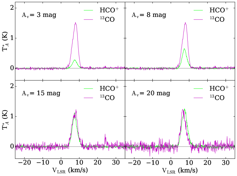
Figure 7: HCO⁺ and ¹³CO spectra are plotted for S254 with increasing $A_{\rm V}$ value for S254. ¹³CO becomes optically thick in higher column densities.

5 Discussion

5.1 Comparison with Inner Galaxy targets

A preliminary comparison between the outer and inner Galaxy targets can provide hints about the effects of Galactic environment. In their study of 6 inner Galaxy clouds with HCN and HCO⁺($J=1\rightarrow 0$), Evans et al. (2020) found a significant amount of luminosity from the diffuse part of the clouds. That is also true for the outer Galaxy clouds, but the fraction of luminosity arising inside the $\mbox{$A_{\rm V}$}\geq 8$ mag or the BGPS region is larger in the outer Galaxy clouds. Also, the behavior of individual tracers differ in both regimes. For inner Galaxy clouds, the average ratio $\langle\mbox{$f_{\rm L}$}(\mbox{{\rm HCO}${}^{+}$})/\mbox{$f_{\rm L}$}(\mbox{{\rm HCN}})\rangle=1.14\pm 0.18$ for $\mbox{$A_{\rm V}$}\geq 8\ \mathrm{mag}$ criterion compared to $0.83\pm 0.10$ for the outer Galaxy clouds. For inner Galaxy clouds $f_{\rm L}$(HCO⁺) is greater than $f_{\rm L}$(HCN), but for the outer Galaxy the order is opposite.

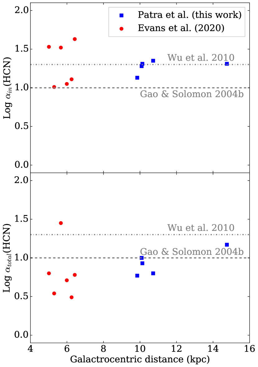
Figure 8: Variation of conversions factors $\mathrm{Log\ \mbox{$\alpha_{\rm in}$}(\mbox{{\rm HCN}})}$ and $\mathrm{Log\ \mbox{$\alpha_{\rm tot}$}(\mbox{{\rm HCN}})}$ for inner and outer Galaxy targets with Galactocentric  distance($R_{G}$).

Evans et al. (2020) also calculated the conversion factor between $M_{\rm dense}$ measured by millimeter-wave continuum data and luminosity coming from the dense region. For inner Galaxy clouds $\alpha_{\rm in}$(HCN) is $20^{+16}_{-9}$ $\mathrm{\mbox{M${}_{\odot}$}(K\ km\ s^{-1}\ pc^{2})^{-1}}$, whereas it is $19^{+3.8}_{-3.2}$ $\mathrm{\mbox{M${}_{\odot}$}(K\ km\ s^{-1}\ pc^{2})^{-1}}$ for outer Galaxy clouds. Considering the whole cloud, the mass-luminosity conversion factor, $\alpha_{\rm tot}$(HCN) was $6.2^{+6.6}_{-3.0}$ $\mathrm{\mbox{M${}_{\odot}$}(K\ km\ s^{-1}\ pc^{2})^{-1}}$ for inner Galaxy clouds and $\alpha_{\rm tot}$(HCN) is $8.5^{+3.8}_{-2.6}$ $\mathrm{\mbox{M${}_{\odot}$}(K\ km\ s^{-1}\ pc^{2})^{-1}}$ for outer Galaxy clouds. From the above values, we can see that $\alpha_{\rm tot}$ and $\alpha_{\rm in}$ for outer Galaxy clouds are consistent with inner Galaxy values. Figure 8 shows the variation of conversion factors with $R_{G}$ for both the set of targets. However, the mean density probed depends on heliocentric distance, and the inner Galaxy clouds are on average farther away. The high outlier in the lower panel of Figure 8 is an inner Galaxy cloud that had very strong self-absorption in HCN, lowering the line luminosity and raising $\alpha_{\rm tot}$(HCN). Bigger samples are needed to understand all the effects.

5.2 Potential Impact of metallicity on fractional Luminosity?

HCN and HCO⁺ are linear molecules with large dipole moments and similar energy levels, but differing in the elemental compositions ($\mathrm{N}$ versus $\mathrm{O}$). This difference in chemical structure makes them sensitive to the chemistry of the interstellar medium. Hence we can expect a connection between the abundance ratio of $\mathrm{N/O}$ and $\mathrm{\mbox{{\rm HCN}}/\mbox{{\rm HCO}${}^{+}$}}$ (Braine et al., 2017). The ratio of total luminosities, $L(\mbox{{\rm HCO}${}^{+}$})/L(\mbox{{\rm HCN}})$, averaged in the logs, is 0.98 for outer Galaxy clouds, while this factor is 0.56 for inner Galaxy targets (Evans et al., 2020). The higher value in the outer Galaxy is consistent with the extragalactic studies on low metallicity systems (1.8-3, LMC, SMC (Chin et al., 1997; Galametz et al., 2020); 1.1-2.8, IC 10 (Nishimura et al., 2016; Braine et al., 2017; Kepley et al., 2018); 1.1-2.5, M33 (Buchbender et al., 2013; Braine et al., 2017); 1.2, M31 (Brouillet et al., 2005)). So, in the low metallicity environments HCO⁺ is as luminous as HCN but less concentrated in dense regions compared to high metallicity regions.

The $f_{\rm L}$ values based on $A_{\rm V}$ analysis increase with the metallicity (Figure 3), but $f_{\rm L}$ values based on BGPS analysis do not. A possible reason for this difference is that we use $\mathrm{[\mbox{${}^{12}$CO}]/[\mbox{${}^{13}$CO}]}$ ratio in the derivation of molecular hydrogen column density ($\rm N(H_{2})$) map (see 4.1), which is a function of $R_{G}$ and indirectly related to metallicity. For BGPS, the same opacity value is used regardless of metallicity, so the metallicity effect is not incorporated there. This study hints at interesting trends with Galactic environment and indicates the need for a larger sample to study it further.

6 Conclusions

In this paper, we study 7 outer Galaxy star-forming regions with HCN and HCO⁺ $J=1\rightarrow 0$ transitions obtained from TRAO 14-m telescope and compare these dense line tracers with extinction, 1.1 mm thermal dust continuum emission (BGPS), and dust column density from Herschel. The results are summarized below.

1. The luminosity coming from the ‘dense’ region based on extinction criteria and BGPS mask maps (indicated as in) is prominent for most of the clouds, but there are significant amounts of luminosity coming from outside the ‘dense’ region (indicated as out) for most of the clouds. The fraction of the total line luminosity arising from the dense region, as indicated by both the BGPS and extinction maps, is higher in HCN, followed by HCO⁺ and ¹³CO. The HCN emission is generally less extended than the HCO⁺ emission.

2. In the outer Galaxy, HCO⁺ is as luminous as HCN, but HCO⁺ is less concentrated in the dense regions; these are the opposite of the trends in the inner Galaxy.

3. Both HCN and HCO⁺ show better agreement with millimeter continuum emission than they do with the extinction criterion for the clouds having BGPS data. The dense line tracers in S212 and S228 do not agree with the extinction criterion.

4. The fraction of line luminosity arising from the dense region based on extinction criterion increases with metallicity, but no such variation for the analysis based on millimeter continuum (Figure 3). For lower metallicity targets, the fraction of the luminosity of the three tracers (HCN, HCO⁺, and ¹³CO) arising in high extinction regions are comparable, but all are low.

5. For 5 clouds, we estimate the mass conversion factor ($\alpha_{\rm in}$) between dense gas mass ($M_{\rm dense}$) arising from BGPS mask region and the line luminosities of HCN, HCO⁺, both within that region ($\alpha_{\rm in}$) and for the whole cloud ($\alpha_{\rm tot}$) in §4.3. The $\alpha_{\rm tot}$ value is consistent with the literature value used in extragalactic studies ($10\ \mbox{M${}_{\odot}$}\ (\rm K\ km\ s^{-1}\ pc^{2})^{-1}$, Gao & Solomon (2004b)), while the $\alpha_{\rm in}$ value is consistent with those found in studies of dense Galactic clumps (Wu et al., 2010). Also, the theoretical value obtained by Onus et al. (2018) for HCN is consistent with either our $\alpha_{\rm in}$(HCN) or $\alpha_{\rm tot}$(HCN).

6. We measure the line-to-mass ratio ($W(Q)/\mbox{$A_{\rm V}$}$) for the 3 targets (S228, S252 and S254) with column densities from Herschel (§4.4). The ¹³CO traces column density well over the range $\mbox{$A_{\rm V}$}=4-10$ mag, but HCN and HCO⁺ trace it better for higher $A_{\rm V}$, confirming the view that dense line tracers (HCN and HCO⁺) are more sensitive to the high column density regions than is ¹³CO.

Table 1: Sample of Clouds

Target	$l$	$b$	$R_{G}$	$D$		$M_{\rm cloud}$	SpT	12+log(O/H)	Map Size	$A_{\rm V}$
	(deg)	(deg)	(kpc)	(kpc)		($10^{4}$ M⊙)	(Ref)	(Ref)	($\ \ {}^{\prime}\ \times\ \ ^{\prime}$)	(mag)
S206	$150.5886$	$-0.8570$	$10.88^{+0.25}_{-0.26}$	$2.96^{+0.17}_{-0.15}$		$18.5$	O4V (1)	8.37 (8)	15 $\times$ 15	1.0
S208	$151.3098$	$1.9045$	$11.87^{+0.37}_{-0.34}$	$4.02^{+0.27}_{-0.25}$		$6.8$	B0V (2)	8.43 (8)	10 $\times$ 20	0.3
S212	$155.3375$	$2.6345$	$14.76\pm 1.30$	$6.65^{+1.36}_{-1.26}$		$19.0$	O7 (3)	8.34 (9)	13 $\times$ 14	0.5
S228	$169.1432$	$-1.0475$	$10.72\pm 0.19$	$2.56\pm 0.09$		$11.6$	O8V (4)	8.39 (8)	11 $\times$ 33	0.4
S235	$173.6682$	$2.7799$	$9.85^{+0.16}_{-0.17}$	$1.66\pm 0.07$		41.1	O9.5V (5)	8.54 (8)	30 $\times$ 30	1.5
S252	$189.8418$	$0.3156$	$10.09^{+0.12}_{-0.11}$	$1.92^{+0.12}_{-0.11}$		49.0	O6.5V,O9.5V,B V (6)	8.51 (8)	30 $\times$ 30	1.5
S254	$192.7935$	$0.0290$	$10.13\pm 0.21$	$1.96^{+0.12}_{-0.09}$		51.5	O9.5V,B0.5V (7)	8.69 (8)	50 $\times$ 34	1.5

Data availability:

Note. — (1)Maíz Apellániz et al. (2016), (2)Moffat et al. (1979), (3)Sota et al. (2014), (4)Chini & Wink (1984), (5)Georgelin et al. (1973), (6)Jose et al. (2012), (7)Ojha et al. (2011), (8)Wang et al. (2018), (9)Méndez-Delgado et al. (2022)

Table 2: Line Luminosities versus $\mbox{$A_{\rm V}$}\geq 8\ \mbox{mag}$

Source	$N_{\rm{in}}/N_{\rm tot}$	Log $L_{\rm tot}$	Log $L_{\rm in}$	$f_{\rm L}$	Log $L_{\rm tot}$	Log $L_{\rm in}$	$f_{\rm L}$	Log $L_{\rm tot}$	Log $L_{\rm in}$	$f_{\rm L}$
		HCN	HCN	HCN	HCO+	HCO+	HCO+	13CO	13CO	13CO
S206	0.067	$1.88^{+0.05}_{-0.05}$	$1.14^{+0.05}_{-0.05}$	0.180(0.008)	$1.84^{+0.05}_{-0.05}$	$1.05^{+0.05}_{-0.05}$	0.164(0.006)	$2.54^{+0.05}_{-0.05}$	$1.76^{+0.05}_{-0.05}$	0.167(0.004)
S208	0.061	$1.31^{+0.06}_{-0.06}$	$0.63^{+0.06}_{-0.06}$	0.209(0.011)	$1.39^{+0.05}_{-0.06}$	$0.62^{+0.05}_{-0.06}$	0.170(0.004)	$2.04^{+0.05}_{-0.06}$	$1.18^{+0.07}_{-0.07}$	0.138(0.014)
S212	$\cdots$	$1.89^{+0.15}_{-0.21}$	$\cdots$	$\cdots$	$1.95^{+0.15}_{-0.21}$	$\cdots$	$\cdots$	$2.49^{+0.15}_{-0.21}$	$\cdots$	$\cdots$
S228	0.008	$1.40^{+0.05}_{-0.05}$	$-0.44^{+0.08}_{-0.09}$	0.014(0.003)	$1.29^{+0.04}_{-0.05}$	$-0.75^{+0.10}_{-0.13}$	0.009(0.002)	$2.77^{+0.03}_{-0.03}$	$1.02^{+0.07}_{-0.08}$	0.018(0.003)
S235	0.164	$2.45^{+0.04}_{-0.04}$	$2.18^{+0.03}_{-0.04}$	0.537(0.011)	$2.43^{+0.03}_{-0.04}$	$2.10^{+0.03}_{-0.04}$	0.471(0.007)	$3.09^{+0.03}_{-0.04}$	$2.64^{+0.03}_{-0.04}$	0.355(0.002)
S252	0.265	$2.53^{+0.05}_{-0.05}$	$2.35^{+0.05}_{-0.05}$	0.661(0.025)	$2.48^{+0.05}_{-0.05}$	$2.27^{+0.05}_{-0.05}$	0.608(0.010)	$3.32^{+0.05}_{-0.05}$	$3.08^{+0.05}_{-0.05}$	0.570(0.003)
S254	0.107	$2.50^{+0.05}_{-0.04}$	$2.16^{+0.05}_{-0.04}$	0.459(0.008)	$2.49^{+0.05}_{-0.04}$	$2.06^{+0.05}_{-0.04}$	0.371(0.006)	$3.21^{+0.05}_{-0.04}$	$2.64^{+0.05}_{-0.04}$	0.269(0.002)
Mean	0.112	1.99	1.34	0.343	1.98	1.22	0.299	2.78	2.05	0.253
Std Dev.	0.083	0.48	1.01	0.225	0.47	1.07	0.204	0.42	0.78	0.177
Median	0.087	1.89	1.65	0.334	1.95	1.56	0.271	2.77	2.20	0.218

Note. — 1. Units of luminosities are K km s^-1pc².

Table 3: Line Luminosities versus BGPS Emission

Source	$N_{\rm{in}}/N_{\rm tot}$	Log $L_{\rm tot}$	Log $L_{\rm in}$	$f_{\rm L}$	Log $L_{\rm tot}$	Log $L_{\rm in}$	$f_{\rm L}$	Log $L_{\rm tot}$	Log $L_{\rm in}$	$f_{\rm L}$
		HCN	HCN	HCN	HCO+	HCO+	HCO+	13CO	13CO	13CO
S212	0.352	$1.89^{+0.15}_{-0.21}$	$1.75^{+0.15}_{-0.21}$	0.728(0.045)	$1.95^{+0.15}_{-0.21}$	$1.80^{+0.15}_{-0.21}$	0.717(0.025)	$2.49^{+0.15}_{-0.21}$	$2.06^{+0.15}_{-0.21}$	0.376(0.017)
S228	0.049	$1.40^{+0.05}_{-0.05}$	$0.84^{+0.03}_{-0.03}$	0.277(0.027)	$1.29^{+0.04}_{-0.05}$	$0.89^{+0.03}_{-0.03}$	0.391(0.034)	$2.77^{+0.03}_{-0.03}$	$1.60^{+0.04}_{-0.04}$	0.068(0.004)
S235	0.118	$2.45^{+0.04}_{-0.04}$	$2.08^{+0.03}_{-0.04}$	0.433(0.009)	$2.43^{+0.03}_{-0.04}$	$2.02^{+0.03}_{-0.04}$	0.386(0.006)	$3.09^{+0.03}_{-0.04}$	$2.49^{+0.03}_{-0.04}$	0.248(0.001)
S252	0.165	$2.53^{+0.05}_{-0.05}$	$2.26^{+0.05}_{-0.05}$	0.533(0.014)	$2.48^{+0.05}_{-0.05}$	$2.18^{+0.05}_{-0.05}$	0.496(0.008)	$3.32^{+0.05}_{-0.05}$	$2.90^{+0.05}_{-0.05}$	0.381(0.002)
S254	0.085	$2.50^{+0.05}_{-0.04}$	$2.12^{+0.05}_{-0.04}$	0.418(0.007)	$2.49^{+0.05}_{-0.04}$	$2.01^{+0.05}_{-0.04}$	0.331(0.005)	$3.21^{+0.05}_{-0.04}$	$2.53^{+0.05}_{-0.04}$	0.208(0.001)
Mean	0.154	2.15	1.81	0.478	2.13	1.78	0.464	2.97	2.32	0.256
Std Dev.	0.106	0.44	0.51	0.149	0.46	0.46	0.137	0.31	0.50	0.116
Median	0.118	2.45	2.08	0.433	2.43	2.01	0.391	3.09	2.49	0.248

Note. — 1. Units of luminosities are K km s^-1pc².

Table 4: $M_{\rm dense}$ versus Luminosities

Source	$\mathrm{Log\ \mbox{$M_{\rm dense}$}}$	Log $L_{\rm tot}$	Log $L_{\rm in}$	$\mathrm{Log\ \alpha_{tot}}$	$\mathrm{Log\ \alpha_{in}}$	Log $L_{\rm tot}$	Log $L_{\rm in}$	$\mathrm{Log\ \alpha_{tot}}$	$\mathrm{Log\ \alpha_{in}}$
	M⊙	HCN	HCN	HCN	HCN	HCO+	HCO+	HCO+	HCO+
S212	$3.06^{+0.16}_{-0.25}$	$1.89^{+0.15}_{-0.21}$	$1.75^{+0.15}_{-0.21}$	$1.17\pm 0.09$	$1.31\pm 0.08$	$1.95^{+0.15}_{-0.21}$	$1.80^{+0.15}_{-0.21}$	$1.11\pm 0.08$	$1.26\pm 0.08$
S228	$2.19^{+0.07}_{-0.08}$	$1.40^{+0.05}_{-0.05}$	$0.84^{+0.03}_{-0.03}$	$0.80\pm 0.07$	$1.35\pm 0.06$	$1.29^{+0.04}_{-0.05}$	$0.89^{+0.03}_{-0.03}$	$0.90\pm 0.07$	$1.31\pm 0.06$
S235	$3.22^{+0.05}_{-0.05}$	$2.45^{+0.04}_{-0.04}$	$2.08^{+0.03}_{-0.04}$	$0.77\pm 0.04$	$1.13\pm 0.03$	$2.43^{+0.03}_{-0.04}$	$2.02^{+0.03}_{-0.04}$	$0.79\pm 0.04$	$1.20\pm 0.03$
S252	$3.53^{+0.06}_{-0.07}$	$2.53^{+0.05}_{-0.05}$	$2.26^{+0.05}_{-0.05}$	$1.00\pm 0.04$	$1.28\pm 0.04$	$2.48^{+0.05}_{-0.05}$	$2.18^{+0.05}_{-0.05}$	$1.05\pm 0.04$	$1.35\pm 0.04$
S254	$3.43^{+0.06}_{-0.06}$	$2.50^{+0.05}_{-0.04}$	$2.12^{+0.05}_{-0.04}$	$0.93\pm 0.04$	$1.31\pm 0.04$	$2.49^{+0.05}_{-0.04}$	$2.01^{+0.05}_{-0.04}$	$0.93\pm 0.04$	$1.41\pm 0.04$
Mean	3.09	2.15	1.81	0.93	1.28	2.13	1.78	0.96	1.31
Std Dev.	0.53	0.44	0.51	0.16	0.08	0.46	0.46	0.13	0.08
Median	3.22	2.45	2.08	0.93	1.31	2.43	2.01	0.93	1.31

Note. — 1. Units of luminosities are K km s^-1pc².

2. Units of conversion factors are $\mbox{M${}_{\odot}$}\ (\rm K\ km\ s^{-1}\ pc^{2})^{-1}$

Appendix A Target Details

All of the sources were identified in the second catalog of visible H II regions by Sharpless (1959).

A.1 Sh2-206

Sh2-206 (hereafter S206) was mapped with the center position $l=150.5886$, $b=-0.8570$ with a map size $15^{\prime}\times 15^{\prime}$. This H II region is not excited by a cluster, but by a single massive star BD$+50886$ (Georgelin et al., 1973). An ionization front forms the bright central region of this target and it surrounds the O4V exciting star to the south and west (Deharveng et al., 2000). The heliocentric distance of this region is $2.96^{+0.17}_{-0.15}$ kpc, measured from the parallax information of the massive star and the Galactocentric distance is $\mbox{$R_{G}$}=10.88^{+0.25}_{-0.26}$ kpc (Méndez-Delgado et al., 2022).

We use the velocity range -27 to -19 km s^-1 to produce the column density map from ¹³CO and integrated intensity map for HCO⁺. For HCN we use the velocity range -34 to -14 km s^-1 for HCN integrated intensity map. The presence of a dense region ($\mbox{$A_{\rm V}$}\geq 8$ mag) is indicated with the white contour on top of the integrated intensity of HCN and HCO⁺in Figure 1(S206). There is strong detection of HCN and HCO⁺ emission in both in and out regions for extinction in the spectrum plots (Figure 2a). The $f_{\rm L}$ value based on $A_{\rm V}$ analysis is higher for HCN, followed by ¹³CO and HCO⁺. This target lacks data in millimeter-wave continuum and Herschel.

A.2 Sh2-208

Sh2-208 (hereafter S208) was mapped with center position $l=151.3098,\ b=1.9045$ with a map size $10^{\prime}\times 20^{\prime}$. This H II region is located at a heliocentric distance of $4.02_{+0.27}^{-0.25}$ kpc in an interarm island between the Cygnus and Perseus arms (Yasui et al., 2016) and the corresponding Galactocentric distance is $11.87_{+0.37}^{-0.34}$ kpc. This HII region is located in a sequential star forming region and the probable dominant star is GSC 03719-00517 (Yasui et al., 2016).

We use the velocity range -32 to -28 km s^-1 to produce the column density map from ¹³CO and integrated intensity map for HCO⁺. For HCN we use the velocity range -40 to -23 km s^-1 for integrated intensity map. Figure 1 shows the integrated intensity plot of HCN and HCO⁺, and the white contours show the area above $\mbox{$A_{\rm V}$}=8$ mag. The extinction criterion of dense gas is in good agreement with the emission of HCN and HCO⁺. Figure 1(b) shows strong emission is coming from the in region for both the lines.

A.3 Sh2-212

Sh2-212 (hereafter S212) is a bright optically-visible HII region, ionized by a cluster (NGC 1624) containing an O7 type star. S212 appears circular in the optical band around the central cluster. The molecular cloud appears as a semi-circular shape in the southern part of the region. The region contains multiple substructures and indicates that it is evolving in a non-homogeneous medium (Deharveng et al., 2008). This region is a likely example of the collect-and-collapse process triggering massive star formation (see Deharveng et al. 2008; Jose et al. 2011 for details).

Our map covered a region of $13^{\prime}\times 14^{\prime}$ centered on $l=155.3375$, $b=2.6345$. This target lies $\sim 300$ pc above the Galactic plane. The heliocentric distance is $6.65_{+1.36}^{-1.26}$ kpc (Méndez-Delgado et al., 2022). This target has the highest Galactocentric distance ($14.76\pm 1.30$ kpc) in the sample and lowest metallicity.

To derive the column density map from ¹³CO and for the integrated intensity map of HCO⁺, we use the velocity integration range -39 to -30.5 km s^-1. For HCN we use the velocity range -44 to -26 km s^-1 for integrated intensity map. Figure 1 (S212) shows the integrated intensity plots of HCN and HCO⁺. For this target there is no region with $\mbox{$A_{\rm V}$}\geq 8$ mag, so there is no white contour present in the figure. But the position of BGPS mask (shown in black contours) and HCN, HCO⁺ shows good agreement. Figure 2(c) shows the spectra for both extinction and BGPS based analysis.

A.4 Sh2-228

Sh2-228 (hereafter S228) was mapped in Galactic co-ordinate with the center position $l=169.1432$, $b=-1.0475$ with a map size $11^{\prime}\times 33^{\prime}$. This H II region is located on the Perseus arm near the large Auriga OB1 association. It is a vast region in which star formation is active. A young cluster IRAS 05100+3723 is associated with the H II region S228 (Yadav et al., 2022). The heliocentric distance of this target is $2.56\pm 0.09$ kpc and the corresponding Galactocentric distance $\mbox{$R_{G}$}=10.72\pm 0.19$ kpc.

To derive the column density map from ¹³CO and for the integrated intensity map of HCO⁺, we use the velocity integration range -12 to -3.5 km s^-1. For HCN we use the velocity range -16 to 2 km s^-1for integrated intensity map. Figure 1(S228) shows the position of $\mbox{$A_{\rm V}$}\geq 8$ mag region and BGPS clumps positions with white and black contours respectively on the integrated intensity maps of HCN and HCO⁺. The emission of HCN and HCO⁺ show good agreement with the BGPS position, but there is no strong emission from HCN, HCO⁺ in the $\mbox{$A_{\rm V}$}\geq 8$ mag region (see spectra in Figure 2(d) ). The lines of ¹³CO in the region of the BGPS peak are slightly below the value corresponding to $\mbox{$A_{\rm V}$}=8$, instead indicating $\mbox{$A_{\rm V}$}=6$ or 7 mag. There are two peaks in the Herschel column density maps, one at the position of BGPS clump and the other below the region where ¹³CO peaks. The lack of strong ¹³CO emission at a peak of BGPS, HCN, and HCO⁺ is unusual. We examined the spectra of ¹³CO at the BGPS peak for evidence of self-absorption, but none was obvious. The $f_{\rm L}$ value based on BGPS analysis is higher for HCN, followed by HCO⁺ and ¹³CO. The line-to-mass ratio versus dust-based extinction plot (Figure 6a) shows that HCO⁺ and HCN are better tracers in the dense region than ¹³CO.

A.5 Sh2-235

Sh2-235 (hereafter S235) is an extended H II region with active star formation and it is located in the Perseus spiral arm (Heyer et al., 1996). This star forming region consists of “S235main” and S235A, S235B, and S235C regions (hereafter “S235ABC”) (Dewangan & Anandarao, 2011). A single massive star BD$+351201$ of O9.5V type is ionizing the “S235main”, while the compact H II regions in “S235ABC” regions are excited by B1V–B0.5V stars (Chavarría et al. (2014); Dewangan & Ojha (2017) and references therein). This cloud has two velocity components, “S235main” with velocity range $-24$ to $-18$ km s^-1 and “S235ABC” with velocity range $-18$ to $-13$ km s^-1. These two clouds are interconnected by a bridge feature with less intensity (Evans & Blair, 1981; Dewangan & Ojha, 2017). This region is also known for the star formation activities influenced by the cloud-cloud collision mechanism (Dewangan & Ojha, 2017).

We mapped $30^{\prime}\times 30^{\prime}$ region with the center $l=173.6682$, $b=2.7799$. The heliocentric distance is $1.66\pm 0.07$ kpc, derived from the parallax information of the ionizing star BD$+351201$ from Gaia EDR3 data. The corresponding Galactocentric distance $\mbox{$R_{G}$}=9.85_{+0.16}^{-0.17}$ kpc (Méndez-Delgado et al., 2022).

To derive the column density map from ¹³CO and for the integrated intensity map of HCO⁺, we use the velocity integration range -24.5 to -12 km s^-1. For HCN we use the velocity range -32 to -7 km s^-1 for integrated intensity map. The 2 velocity component at -20 km s^-1 and -17.3 km s^-1 are not separable at some positions, so the integration range we consider covers both the components. All the tracers (HCN, HCO⁺, extinction and BGPS emission) agree with each other (Figure 1(S235)). The white contour ($\mbox{$A_{\rm V}$}\geq 8$ mag) covers larger area than the BGPS region (black contours). There are strong detections of HCN and HCO⁺ emission in both in and out regions for extinction and BGPS in the spectrum plots (Figure 2e).

A.6 Sh2-252

Sh2-252 (hereafter S252), also known as NGC 2175 is an optically bright, evolved H II region with size $\sim 20$ pc. This region is part of Gemini OB1 association. The central star HD 42088 of spectral type O6.5 V is the main ionizing source (Jose et al., 2012). This region also contains four compact H II (CH II) regions (A, B, C and E) (Felli et al., 1977) and powered by ionizing sources with spectral type later than O6.5V in each of them. This cloud has several regions of recent star formation activity.

Table 4 of Jose et al. (2012) listed the massive stars in each of these clumps with their spectral types. We take the parallax information of those stars (ID 1-6 and 11-12 from the Table 4 of Jose et al. 2012) from Gaia EDR3 and calculate the distance by averaging all the parallaxes. The distance is $1.92^{+0.12}_{-0.11}$ kpc and the corresponding Galactocentric distance $\mbox{$R_{G}$}=10.09_{+0.12}^{-0.11}$ kpc. This source was mapped with center position $l=189.8418$, $b=0.3156$ with a map size $30^{\prime}\times 30^{\prime}$.

We use the velocity range 2 to 14 km s^-1 to produce the column density map from ¹³CO and integrated intensity map of HCO⁺. For HCN we use the velocity range -4 to 20 km s^-1 for integrated intensity map. Figure1(S252) shows the contour of $\mbox{$A_{\rm V}$}\geq 8$ mag (in white) and BGPS clumps (in black) in the integrated intensity maps of HCN, HCO⁺ and all the tracers are in good agreement. There is strong detection of HCN and HCO⁺ emission in both in and out regions for extinction and BGPS in the spectrum plots (Figure 2f).

A.7 Sh2-254 Complex

This region is a complex with five H II regions (Sh2-254, Sh2-255, Sh2-256, Sh2-257 and Sh2-258) and part of Gemini OB association. This is a sequential star-forming region triggered by expanding H II regions (Bieging et al., 2007; Chavarría et al., 2008; Ojha et al., 2011). These five evolved H II regions are projected on a 20 pc long filament. The exciting stars present in S254, S255, S256, S257 and S258 have spectral types of O9.6 V, B0.0 V, B0.9 V, B0.5V and B1.5V Chavarría et al. (2008). Ladeyschikov et al. (2021) studied the link between the gas-dust constituents and the young stellar objects (YSOs) distribution. They identified high-density gas (HCO⁺($J=1\rightarrow 0$) and CS($J=2\rightarrow 1$)) in the inter-clump bridge position between the star clusters S255N and S256-south and suggested that the clusters have an evolutionary link. We mapped $50^{\prime}\times 34^{\prime}$ area of Sh2-254 complex with the center position $l=192.7935$, $b=0.0290$. The Galactocentric distance is $\mbox{$R_{G}$}=10.13\pm 0.21$ kpc and the heliocentric distance is $1.96_{+0.12}^{-0.09}$ kpc based on GAIA EDR3 (Méndez-Delgado et al., 2022).

We use the velocity range 4.5 to 11.5 km s^-1 to produce the column density map from ¹³CO and integrated intensity map of HCO⁺. For HCN we use the velocity range -4 to 17 km s^-1 for integrated intensity map. The contour plot (Figure 1(S254)) for this cloud shows good agreement among HCN, HCO⁺, extinction and BGPS. There are strong detections of HCN and HCO⁺ emission in both in and out regions for extinction and BGPS in the spectrum plots (Figure 2g).

Appendix B Reduction Details

Our standard procedure of data reduction is as follows. First we check the data to find the velocity intervals with significant emission ($v_{win}$). Then we exclude the window of velocity having emission while removing a baseline order, also using only enough velocity range to get good baseline on each end ($v_{sp}$). After that we made spectral cubes in FITS format for further analysis. The values of the total velocity range and excluded windows are shown in Table LABEL:lineprops. We experimented on the velocity range ($v_{sp}$) and baseline order to get the best fit.

Change in baseline order

First we have experimented on the baseline order removal. For a same target, by keeping $v_{win}$ and $v_{sp}$ same, we tried both first and second order baselines. For most of the cases, the second order baseline removal was superior.

Change in $v_{sp}$ range

Further we change the velocity range of $v_{sp}$ (while keeping the baseline removal order fixed) for each target with 2 different set - (i) wider range of $v_{sp}$ and (ii) narrow range of $v_{sp}$ to see the effect on final results.

In the final analysis, we used baselines of order 2 with wider range of $v_{sp}$. Table LABEL:tab:reduction shows the choice of velocity ranges and lists the positions of all the peaks in terms of offset from the center of the map, with offsets in Galactic coordinates.

Table 5: Data Reduction Details

Source	Line	$v_{sp}$	$v_{win}$	Peak Offset	Notes
		(km s-1)	(km s-1)	(arcsec)
S206	HCN	-45, 0	-32, -14	280, 280	Peak position 1
S206	HCO+	-45, 0	-27, -19	280, 280	Peak position 1
S206	HCN	-45, 0	-32, -14	180, 120	Peak position 2
S206	HCO+	-45, 0	-27, -19	180, 120	Peak position 2
S206	HCN	-45, 0	-32, -14	-40, -280	Peak position 3
S206	HCO+	-45, 0	-27, -19	-40, -280	Peak position 3
S208	HCN	-55, -5	-40, -23	-100, 200
S208	HCO+	-55, -5	-34, -27	-100, 200
S212	HCN	-60, -10	-44, -26	0, -160	Peak position 1
S212	HCO+	-60, -10	-40, -29	0, -160	Peak position 1
S212	HCN	-60, -10	-44, -26	120, -40	Peak position 2
S212	HCO+	-60, -10	-40, -29	120, -40	Peak position 2
S228	HCN	-30, 20	-16, 3	160, 520
S228	HCO+	-30, 20	-11, -2	160, 520
S235	HCN	-50, 10	-32, -7	-160, 100	Peak position 1
S235	HCO+	-50, 10	-26, -12	-160, 100	Peak position 1
S235	HCN	-50, 10	-32, -7	180, -300	Peak position 2
S235	HCO+	-50, 10	-26, -12	180, -300	Peak position 2
S235	HCN	-50, 10	-32, -7	0, 340	Peak position 3
S235	HCO+	-50, 10	-26, -12	0, 340	Peak position 3
S235	HCN	-50, 10	-32, -7	-180, 360	Peak position 4
S235	HCO+	-50, 10	-26, -12	-180, 360	Peak position 4
S252	HCN	-20, 40	-4, 18	-220, 100	Peak position 1
S252	HCO+	-20, 40	2, 14	-220, 100	Peak position 1
S252	HCN	-20, 40	-4, 20	-120, 120	Peak position 2
S252	HCO+	-20, 40	0, 15	-120, 120	Peak position 2
S252	HCN	-20, 40	-4, 20	400, 60	Peak position 3
S252	HCO+	-20, 40	0, 15	400, 60	Peak position 3
S252	HCN	-20, 40	-4, 20	0, 640	Peak position 4
S252	HCO+	-20, 40	0, 15	0, 640	Peak position 4
S252	HCN	-20, 40	-4, 20	400, -300	Peak position 5
S252	HCO+	-20, 40	0, 15	400, -300	Peak position 5
S252	HCN	-20, 40	-4, 20	-620, -520	Peak position 6
S252	HCO+	-20, 40	0, 15	-620, -520	Peak position 6
S254	HCN	-25, 35	-4, 17	-720, -280	Peak position 1
S254	HCO+	-25, 35	2, 14	-720, -280	Peak position 1
S254	HCN	-25, 35	-4, 17	740, 360	Peak position 2
S254	HCO+	-25, 35	2, 14	740, 360	Peak position 2
S254	HCN	-25, 35	-4, 17	-120, 240	Peak position 3
S254	HCO+	-25, 35	2, 14	-120, 240	Peak position 3
S254	HCN	-25, 35	-4, 17	220, 280	Peak position 4
S254	HCO+	-25, 35	2, 14	220, 280	Peak position 4

Appendix C The H₂ column density map derived from ¹²CO and ¹³CO

To measure the molecular hydrogen (H₂) column density map from ¹²CO and ¹³CO, we assume that both the molecular lines arise from the same region of the clouds. We follow the steps from Ripple et al. (2013) and Pineda et al. (2010). ¹²CO line is optically thick and its isotopologue ¹³CO is optically thin. We assume that they both have same excitation temperature ($T_{ex}$). So we derive the $T_{ex}$ using the peak brightness temperature ($T_{12,pk}$) of the optically thick ¹²CO line.

$$T_{ex}=\frac{5.53}{\mathrm{ln}\left(1+\frac{5.53}{T_{12,pk}+0.83}\right)}$$ (C1)

We derive the optical depth of ¹³CO in the upper rotational state $(J=1)$, $(\tau_{13,1})$ using the main-beam brightness temperature of ¹³CO, $(T_{13})$ and substitute $T_{ex}$ derived from the ¹²CO observations into the following equation

$$\tau_{13,1}(v)=-\mathrm{ln}\Bigg{[}1-\frac{T_{13}(v)}{5.29}\bigg{(}\bigg{[}\mathrm{exp(5.29/T_{ex})-1}\bigg{]}^{-1}-0.16\bigg{)}^{-1}\Bigg{]}$$ (C2)

The optical depth in ¹³CO is then converted into a upper level column density as follows

$$N_{U}=\frac{8\pi k\nu^{2}}{hc^{3}A_{UL}C(T_{ex})}\Bigg{[}\frac{\int\tau_{13,1}(v)dv}{\int(1-\mathrm{exp}(-\tau_{13,1}(v)))dv}\Bigg{]}\int T_{13}(v)dv$$ (C3)

where $A_{UL}$ is the Eienstein A coefficient and $\nu$ is the frequency of the $J=1\rightarrow 0$ transition. Here we incorporated the correction factor $C(T_{ex})=\left(1-\frac{e^{T_{0}/T_{ex}}-1}{e^{T_{0}/T_{bg}}-1}\right)$, which is equal to unity in the limit $T_{bg}\to 0$.

The column density of the upper level $(J=1)$ is related to the total ¹³CO column density by the following equation

$$N_{\mbox{${}^{13}$CO}}=N_{U}\frac{Z}{2J+1}\mathrm{exp}[hB_{0}J(J+1)/kT_{ex}]$$ (C4)

To calculate the upper level column density, we use the rotational constant for ¹³CO $B_{0}=5.51\times 10^{10}$ s^-1 and use the partition function $Z$ which is defined as

$$Z=\sum_{J=0}^{\infty}(2J+1)\mathrm{exp}[-hB_{0}J(J+1)/kT_{ex}]$$ (C5)

This equation using a single $T_{ex}$ assumes that all levels have the same $T_{ex}$ (the so-called LTE approximation).

The assumption that $T_{ex}$ is the same for ¹³CO and ¹²CO (in equation C1) can fail. If the excitation temperature of ¹³CO is higher (lower) than that of ¹²CO, the optical depth of ¹³CO will be over-estimated (under-estimated) when the $T_{ex}$ from ¹²CO is used in equation C2. For clouds heated from the outside by hot stars, the front of the cloud is likely to be hotter than the inside, leading to an underestimate of the optical depth of ¹³CO.

Roueff et al. (2021) checked the validity of the simple assumption of equal $T_{ex}$ in the Orion B molecular cloud by using Cramer Rao Bound (CRB) technique to estimate different physical properties (column density, excitation temperature, velocity dispersion etc.) in the framework of LTE radiative transfer model. They found that isotopologues had different excitation temperatures; ¹²CO (30 K) had higher $T_{ex}$ than ¹³CO (17 K), so that $T_{ex}(\mbox{${}^{12}$CO})/T_{ex}(\mbox{${}^{13}$CO})\sim 1.7$. If a similar situation applies to the more opaque parts of our clouds, ¹³CO is likely to underestimate the column density.

References

- Astropy Collaboration et al. (2013) Astropy Collaboration, Robitaille, T. P., Tollerud, E. J., et al. 2013, A&A, 558, A33, doi: 10.1051/0004-6361/201322068
- Astropy Collaboration et al. (2018) Astropy Collaboration, Price-Whelan, A. M., Sipőcz, B. M., et al. 2018, AJ, 156, 123, doi: 10.3847/1538-3881/aabc4f
- Balser et al. (2011) Balser, D. S., Rood, R. T., Bania, T. M., & Anderson, L. D. 2011, ApJ, 738, 27, doi: 10.1088/0004-637X/738/1/27
- Barnes et al. (2020) Barnes, A. T., Kauffmann, J., Bigiel, F., et al. 2020, MNRAS, 497, 1972, doi: 10.1093/mnras/staa1814
- Bergin & Langer (1997) Bergin, E. A., & Langer, W. D. 1997, ApJ, 486, 316, doi: 10.1086/304510
- Bieging et al. (2007) Bieging, J. H., Peters, W. L., Vilaro, B. V., Schlottman, K., & Kulesa, C. 2007, in Triggered Star Formation in a Turbulent ISM, ed. B. G. Elmegreen & J. Palous, Vol. 237, 396–396, doi: 10.1017/S1743921307001846
- Bolatto et al. (2013) Bolatto, A. D., Wolfire, M., & Leroy, A. K. 2013, ARA&A, 51, 207, doi: 10.1146/annurev-astro-082812-140944
- Bolocam GPS Team (2020) Bolocam GPS Team. 2020, Bolocam Galactic Plane Survey, IPAC, doi: 10.26131/IRSA482
- Braine et al. (2017) Braine, J., Shimajiri, Y., André, P., et al. 2017, A&A, 597, A44, doi: 10.1051/0004-6361/201629781
- Brouillet et al. (2005) Brouillet, N., Muller, S., Herpin, F., Braine, J., & Jacq, T. 2005, A&A, 429, 153, doi: 10.1051/0004-6361:20034354
- Buchbender et al. (2013) Buchbender, C., Kramer, C., Gonzalez-Garcia, M., et al. 2013, A&A, 549, A17, doi: 10.1051/0004-6361/201219436
- Chavarría et al. (2014) Chavarría, L., Allen, L., Brunt, C., et al. 2014, MNRAS, 439, 3719, doi: 10.1093/mnras/stu224
- Chavarría et al. (2008) Chavarría, L. A., Allen, L. E., Hora, J. L., Brunt, C. M., & Fazio, G. G. 2008, ApJ, 682, 445, doi: 10.1086/588810
- Chin et al. (1997) Chin, Y. N., Henkel, C., Whiteoak, J. B., et al. 1997, A&A, 317, 548. https://arxiv.org/abs/astro-ph/9606081
- Chini & Wink (1984) Chini, R., & Wink, J. 1984, Astronomy and Astrophysics, 139, L5
- Deharveng et al. (2008) Deharveng, L., Lefloch, B., Kurtz, S., et al. 2008, A&A, 482, 585, doi: 10.1051/0004-6361:20079233
- Deharveng et al. (2000) Deharveng, L., Peña, M., Caplan, J., & Costero, R. 2000, MNRAS, 311, 329, doi: 10.1046/j.1365-8711.2000.03030.x
- Dewangan & Anandarao (2011) Dewangan, L. K., & Anandarao, B. G. 2011, MNRAS, 414, 1526, doi: 10.1111/j.1365-2966.2011.18487.x
- Dewangan & Ojha (2017) Dewangan, L. K., & Ojha, D. K. 2017, ApJ, 849, 65, doi: 10.3847/1538-4357/aa8e00
- Dunham et al. (2011) Dunham, M. K., Rosolowsky, E., Evans, Neal J., I., Cyganowski, C., & Urquhart, J. S. 2011, ApJ, 741, 110, doi: 10.1088/0004-637X/741/2/110
- Enoch et al. (2006) Enoch, M. L., Young, K. E., Glenn, J., et al. 2006, ApJ, 638, 293, doi: 10.1086/498678
- Esteban et al. (2017) Esteban, C., Fang, X., García-Rojas, J., & Toribio San Cipriano, L. 2017, MNRAS, 471, 987, doi: 10.1093/mnras/stx1624
- Esteban & García-Rojas (2018) Esteban, C., & García-Rojas, J. 2018, MNRAS, 478, 2315, doi: 10.1093/mnras/sty1168
- Evans & Blair (1981) Evans, N. J., I., & Blair, G. N. 1981, ApJ, 246, 394, doi: 10.1086/158937
- Evans (1989) Evans, Neal J., I. 1989, Rev. Mexicana Astron. Astrofis., 18, 21
- Evans (1999) —. 1999, ARA&A, 37, 311, doi: 10.1146/annurev.astro.37.1.311
- Evans et al. (2014) Evans, Neal J., I., Heiderman, A., & Vutisalchavakul, N. 2014, ApJ, 782, 114, doi: 10.1088/0004-637X/782/2/114
- Evans et al. (2020) Evans, Neal J., I., Kim, K.-T., Wu, J., et al. 2020, ApJ, 894, 103, doi: 10.3847/1538-4357/ab8938
- Felli et al. (1977) Felli, M., Habing, H., & Israel, F. 1977, Astronomy and Astrophysics, 59, 43
- Galametz et al. (2020) Galametz, M., Schruba, A., De Breuck, C., et al. 2020, A&A, 643, A63, doi: 10.1051/0004-6361/202038641
- Gao & Solomon (2004a) Gao, Y., & Solomon, P. M. 2004a, ApJ, 606, 271, doi: 10.1086/382999
- Gao & Solomon (2004b) —. 2004b, ApJS, 152, 63, doi: 10.1086/383003
- Georgelin et al. (1973) Georgelin, Y., Georgelin, Y., & Roux, S. 1973, Astronomy and Astrophysics, 25, 337
- Ginsburg et al. (2013) Ginsburg, A., Glenn, J., Rosolowsky, E., et al. 2013, ApJS, 208, 14, doi: 10.1088/0067-0049/208/2/14
- Gravity Collaboration et al. (2019) Gravity Collaboration, Abuter, R., Amorim, A., et al. 2019, A&A, 625, L10, doi: 10.1051/0004-6361/201935656
- Heiderman et al. (2010) Heiderman, A., Evans, Neal J., I., Allen, L. E., Huard, T., & Heyer, M. 2010, ApJ, 723, 1019, doi: 10.1088/0004-637X/723/2/1019
- Heyer et al. (2022) Heyer, M., Gregg, B., Calzetti, D., et al. 2022, ApJ, 930, 170, doi: 10.3847/1538-4357/ac67ea
- Heyer et al. (1996) Heyer, M. H., Carpenter, J. M., & Ladd, E. F. 1996, ApJ, 463, 630, doi: 10.1086/177277
- Hildebrand (1983) Hildebrand, R. H. 1983, QJRAS, 24, 267
- Hunter (2007) Hunter, J. D. 2007, Computing in Science and Engineering, 9, 90, doi: 10.1109/MCSE.2007.55
- Jacob et al. (2020) Jacob, A. M., Menten, K. M., Wiesemeyer, H., et al. 2020, A&A, 640, A125, doi: 10.1051/0004-6361/201937385
- Jeong et al. (2019) Jeong, I.-G., Kang, H., Jung, J., et al. 2019, Journal of Korean Astronomical Society, 52, 227
- Jiménez-Donaire et al. (2019) Jiménez-Donaire, M. J., Bigiel, F., Leroy, A. K., et al. 2019, ApJ, 880, 127, doi: 10.3847/1538-4357/ab2b95
- Jose et al. (2011) Jose, J., Pandey, A. K., Ogura, K., et al. 2011, MNRAS, 411, 2530, doi: 10.1111/j.1365-2966.2010.17860.x
- Jose et al. (2012) —. 2012, MNRAS, 424, 2486, doi: 10.1111/j.1365-2966.2012.21175.x
- Joye & Mandel (2003) Joye, W. A., & Mandel, E. 2003, in Astronomical Society of the Pacific Conference Series, Vol. 295, Astronomical Data Analysis Software and Systems XII, ed. H. E. Payne, R. I. Jedrzejewski, & R. N. Hook, 489
- Kauffmann et al. (2008) Kauffmann, J., Bertoldi, F., Bourke, T. L., Evans, N. J., I., & Lee, C. W. 2008, A&A, 487, 993, doi: 10.1051/0004-6361:200809481
- Kauffmann et al. (2017) Kauffmann, J., Goldsmith, P. F., Melnick, G., et al. 2017, A&A, 605, L5, doi: 10.1051/0004-6361/201731123
- Kennicutt & Evans (2012) Kennicutt, R. C., & Evans, N. J. 2012, ARA&A, 50, 531, doi: 10.1146/annurev-astro-081811-125610
- Kepley et al. (2018) Kepley, A. A., Bittle, L., Leroy, A. K., et al. 2018, ApJ, 862, 120, doi: 10.3847/1538-4357/aacaf4
- Lacy et al. (2017) Lacy, J. H., Sneden, C., Kim, H., & Jaffe, D. T. 2017, in American Astronomical Society Meeting Abstracts, Vol. 230, American Astronomical Society Meeting Abstracts #230, 215.02
- Lada et al. (2012) Lada, C. J., Forbrich, J., Lombardi, M., & Alves, J. F. 2012, ApJ, 745, 190, doi: 10.1088/0004-637X/745/2/190
- Lada et al. (2010) Lada, C. J., Lombardi, M., & Alves, J. F. 2010, ApJ, 724, 687, doi: 10.1088/0004-637X/724/1/687
- Ladeyschikov et al. (2021) Ladeyschikov, D. A., Kirsanova, M. S., Sobolev, A. M., et al. 2021, MNRAS, 506, 4447, doi: 10.1093/mnras/stab1821
- Liu et al. (2016) Liu, T., Kim, K.-T., Yoo, H., et al. 2016, ApJ, 829, 59, doi: 10.3847/0004-637X/829/2/59
- Maíz Apellániz et al. (2016) Maíz Apellániz, J., Sota, A., Arias, J. I., et al. 2016, ApJS, 224, 4, doi: 10.3847/0067-0049/224/1/4
- Marsh et al. (2015) Marsh, K. A., Whitworth, A. P., & Lomax, O. 2015, MNRAS, 454, 4282, doi: 10.1093/mnras/stv2248
- Marsh et al. (2017) Marsh, K. A., Whitworth, A. P., Lomax, O., et al. 2017, MNRAS, 471, 2730, doi: 10.1093/mnras/stx1723
- Méndez-Delgado et al. (2022) Méndez-Delgado, J. E., Amayo, A., Arellano-Córdova, K. Z., et al. 2022, MNRAS, doi: 10.1093/mnras/stab3782
- Moffat et al. (1979) Moffat, A., Fitzgerald, M., & Jackson, P. 1979, Astronomy and Astrophysics Supplement Series, 38, 197
- Nguyen-Luong et al. (2020) Nguyen-Luong, Q., Nakamura, F., Sugitani, K., et al. 2020, ApJ, 891, 66, doi: 10.3847/1538-4357/ab700a
- Nishimura et al. (2016) Nishimura, Y., Shimonishi, T., Watanabe, Y., et al. 2016, ApJ, 829, 94, doi: 10.3847/0004-637X/829/2/94
- Ojha et al. (2011) Ojha, D. K., Samal, M. R., Pandey, A. K., et al. 2011, ApJ, 738, 156, doi: 10.1088/0004-637X/738/2/156
- Onus et al. (2018) Onus, A., Krumholz, M. R., & Federrath, C. 2018, MNRAS, 479, 1702, doi: 10.1093/mnras/sty1662
- Pety (2018) Pety, J. 2018, in Submillimetre Single-dish Data Reduction and Array Combination Techniques, 11, doi: 10.5281/zenodo.1205423
- Pety et al. (2017) Pety, J., Guzmán, V. V., Orkisz, J. H., et al. 2017, A&A, 599, A98, doi: 10.1051/0004-6361/201629862
- Pineda et al. (2010) Pineda, J. L., Goldsmith, P. F., Chapman, N., et al. 2010, ApJ, 721, 686, doi: 10.1088/0004-637X/721/1/686
- Ripple et al. (2013) Ripple, F., Heyer, M. H., Gutermuth, R., Snell, R. L., & Brunt, C. M. 2013, MNRAS, 431, 1296, doi: 10.1093/mnras/stt247
- Roman-Duval et al. (2016) Roman-Duval, J., Heyer, M., Brunt, C. M., et al. 2016, ApJ, 818, 144, doi: 10.3847/0004-637X/818/2/144
- Rosolowsky et al. (2010) Rosolowsky, E., Dunham, M. K., Ginsburg, A., et al. 2010, ApJS, 188, 123, doi: 10.1088/0067-0049/188/1/123
- Roueff et al. (2021) Roueff, A., Gerin, M., Gratier, P., et al. 2021, A&A, 645, A26, doi: 10.1051/0004-6361/202037776
- Searle (1971) Searle, L. 1971, ApJ, 168, 327, doi: 10.1086/151090
- Sharpless (1959) Sharpless, S. 1959, ApJS, 4, 257, doi: 10.1086/190049
- Shimajiri et al. (2017) Shimajiri, Y., André, P., Braine, J., et al. 2017, A&A, 604, A74, doi: 10.1051/0004-6361/201730633
- Shirley (2015) Shirley, Y. L. 2015, PASP, 127, 299, doi: 10.1086/680342
- Smithsonian Astrophysical Observatory (2000) Smithsonian Astrophysical Observatory. 2000, SAOImage DS9: A utility for displaying astronomical images in the X11 window environment, Astrophysics Source Code Library, record ascl:0003.002. http://ascl.net/0003.002
- Sota et al. (2014) Sota, A., Maíz Apellániz, J., Morrell, N. I., et al. 2014, ApJS, 211, 10, doi: 10.1088/0067-0049/211/1/10
- Stephens et al. (2016) Stephens, I. W., Jackson, J. M., Whitaker, J. S., et al. 2016, ApJ, 824, 29, doi: 10.3847/0004-637X/824/1/29
- The Astropy Collaboration et al. (2022) The Astropy Collaboration, Price-Whelan, A. M., Lian Lim, P., et al. 2022, arXiv e-prints, arXiv:2206.14220. https://arxiv.org/abs/2206.14220
- van der Walt et al. (2011) van der Walt, S., Colbert, S. C., & Varoquaux, G. 2011, Computing in Science and Engineering, 13, 22, doi: 10.1109/MCSE.2011.37
- Vutisalchavakul et al. (2016) Vutisalchavakul, N., Evans, Neal J., I., & Heyer, M. 2016, ApJ, 831, 73, doi: 10.3847/0004-637X/831/1/73
- Wang et al. (2018) Wang, L.-L., Luo, A. L., Hou, W., et al. 2018, PASP, 130, 114301, doi: 10.1088/1538-3873/aadf22
- Wu et al. (2005) Wu, J., Evans, Neal J., I., Gao, Y., et al. 2005, ApJ, 635, L173, doi: 10.1086/499623
- Wu et al. (2010) Wu, J., Evans, Neal J., I., Shirley, Y. L., & Knez, C. 2010, ApJS, 188, 313, doi: 10.1088/0067-0049/188/2/313
- Yadav et al. (2022) Yadav, R. K., Samal, M. R., Semenko, E., et al. 2022, ApJ, 926, 16, doi: 10.3847/1538-4357/ac3a78
- Yasui et al. (2016) Yasui, C., Kobayashi, N., Saito, M., & Izumi, N. 2016, AJ, 151, 115, doi: 10.3847/0004-6256/151/5/115