Relative baryon-dark matter velocities in cosmological zoom simulations

Abstract

Supersonic relative motion between baryons and dark matter due to the decoupling of baryons from the primordial plasma after recombination affects the growth of the first small-scale structures. Large box sizes (greater than a few hundred Mpc) are required to sample the full range of scales pertinent to the relative velocity, while the effect of the relative velocity is strongest on small scales (less than a few hundred kpc). This separation of scales naturally lends itself to the use of ‘zoom’ simulations, and here we present our methodology to self-consistently incorporate the relative velocity in zoom simulations, including its cumulative effect from recombination through to the start time of the simulation. We apply our methodology to a large-scale cosmological zoom simulation, finding that the inclusion of relative velocities suppresses the halo baryon fraction by $46$–$23$ per cent between $z=13.6$ and $11.2$, in qualitative agreement with previous works. In addition, we find that including the relative velocity delays the formation of star particles by $\sim 20~{}\mathrm{Myr}$ on average (of the order of the lifetime of a $\sim 9~{}\mathrm{M}_{\odot}$ Population III star) and suppresses the final stellar mass by as much as $79$ per cent at $z=11.2$.

1 Introduction

The cosmic microwave background (CMB) radiation carries an image of the Universe at the moment of recombination, when the first neutral atoms formed at $z_{\mathrm{rec}}\approx 1089$. Prior to recombination, photons and baryons were tightly coupled and oscillated as a single plasma until they decoupled at $z_{\mathrm{dec}}\approx 1020$. These oscillations, referred to as the baryon acoustic oscillations (BAO), are observed today as fluctuations of the CMB temperature (e.g. Planck Collaboration et al., 2020). Acoustic oscillations in the baryons’ velocity at the moment of their decoupling lead to clumping in the distribution of baryons at later times, resulting in over and underdense regions. The initially tiny perturbations grew under the effect of gravity and are detected today in the distribution of galaxies on the largest cosmological scales (e.g. Alam et al., 2017).

Not only did the plasma oscillations lead to the BAO features in the post-recombination distribution of baryons, they also impacted the baryons’ velocities (Sunyaev & Zeldovich, 1970). Tseliakhovich & Hirata (2010) were the first to point out that the BAO pattern is imprinted in the magnitude of the relative velocity between baryons and dark matter, because the latter was not coupled to the primordial plasma at the time of recombination. At decoupling, the relative velocity had a root-mean-square (RMS) of $\langle v_{\rm bc}^{2}\rangle^{\frac{1}{2}}\approx 30~{}\mathrm{km}~{}\mathrm{s}^{-1}$, or $\sim 10^{-4}\,c$ with $c$ the speed of light. There is a vast separation of scales relevant to the relative velocity. Over scales smaller than a few Mpc (the coherence scale), the relative velocity is roughly constant; however, box sizes greater than a few hundred Mpc are required to properly sample the relative velocity (see Fig. 1 of this work and also fig. 1 in Tseliakhovich & Hirata, 2010). At recombination the sound speed of the baryonic fluid dropped from being relativistic, $\sim c/\sqrt{3}$, to the thermal velocities of hydrogen atoms, $\sim 2\times 10^{-5}c$, which is much smaller than the RMS value of $v_{\rm bc}$. Therefore, on average, at decoupling baryons were travelling with supersonic velocities relative to the underlying potential wells generated by dark matter haloes (Tseliakhovich & Hirata, 2010). The relative velocity remained supersonic all the way down to $z\sim 15$, sourcing shocks and entropy generation (Tseliakhovich & Hirata, 2010; O’Leary & McQuinn, 2012). The amplitude of the velocity field decayed with time as $(1+z)$, and thus the effect weakened as the Universe expanded. For instance, the signature of $v_{\rm bc}$ in the low-$z$ power spectrum of BOSS galaxies (Yoo & Seljak, 2013; Beutler et al., 2017) and the three-point correlation function of BOSS CMASS galaxies was found to be negligible (Slepian & Eisenstein, 2015; Slepian et al., 2018).

In the post-recombination Universe, growth of structure on large cosmological scales is generally described by linear perturbation theory, which follows the evolution of density and velocity fields to the leading order in perturbations. Despite being formally second-order contributions, terms that involve the supersonic relative velocity can actually be as large as the first order terms. Moreover, on scales below the coherence scale, $v_{\rm bc}$ is position-independent and the second-order terms become effectively linear (Tseliakhovich & Hirata, 2010). Using such a ‘quasi-linear’ approach, analytical methods were employed to explore implications of $v_{\rm bc}$ in the cosmological context. Supersonic relative velocities modulate the abundance of minihaloes and their gas content on the BAO scale (e.g. Tseliakhovich & Hirata, 2010; Tseliakhovich et al., 2011; Fialkov et al., 2012; Ahn, 2016; Ahn & Smith, 2018), affecting fluctuations of the 21-cm signal of neutral hydrogen (e.g. Dalal et al., 2010; McQuinn & O’Leary, 2012; Visbal et al., 2012; Fialkov et al., 2013; Cohen et al., 2016; Fialkov et al., 2018; Muñoz, 2019; Cain et al., 2020; Muñoz et al., 2022; Long et al., 2022).

Numerical simulations were used to explore non-linear effects of $v_{\rm bc}$ on scales well below its coherence scale. Such simulations typically employ boxes of several comoving Mpc or less and assume a position-independent velocity field. These simulations demonstrated that $v_{\rm bc}$ suppresses formation of small dark matter haloes (Naoz et al., 2012, 2013; O’Leary & McQuinn, 2012), induces shocks (O’Leary & McQuinn, 2012), affects the formation of first stars (e.g. Maio et al., 2011; Stacy et al., 2011; Greif et al., 2011; Schauer et al., 2019, 2021) and black holes (e.g. Hirano et al., 2017; Schauer et al., 2017), and may even influence shaping globular clusters (Naoz & Narayan, 2014; Chiou et al., 2018; Chiou et al., 2019, 2021; Druschke et al., 2020; Lake et al., 2021).

Finally, a hybrid approach was used to incorporate the non-linear effects into the large-scale cosmological picture by tiling regions of fixed $v_{\rm bc}$ together (e.g. Visbal et al., 2012; Fialkov et al., 2013). In such studies, the distribution of $v_{\rm bc}$ on scales larger than the ‘pixel’ size was generated from the corresponding density field using the continuity equation, while star formation in each ‘pixel’ was calibrated to numerical simulations (Maio et al., 2011; Stacy et al., 2011; Greif et al., 2011; Naoz et al., 2012, 2013). This method was applied to the 21-cm signal of neutral hydrogen revealing enhanced BAO patterns (Visbal et al., 2012; Fialkov et al., 2013).

To fully capture the non-linear effect of $v_{\rm bc}$ in the cosmological context, it is necessary to properly include the velocity effect in the initial conditions of $N$-body and hydrodynamical simulations. Such a task would require an accurate non-linear treatment of dark matter, baryons, and radiation, starting at $z_{\mathrm{rec}}$ and following the growth of structure all the way down to the lowest simulated redshift. This treatment is not possible due to the large dynamical range: the amplitude of density fluctuations at recombination is smaller than the precision of many commonly used integration schemes. Today, state-of-the-art numerical simulations are typically initialised at $z_{\rm ini}\sim 200$ with fields that do not incorporate the effect of the relative velocity.

Recently, Ahn & Smith (2018) introduced a new cosmological initial condition generator bccomics, based on a code that solves the quasi-linear equations between $z_{\rm rec}$ and $z_{\rm ini}$ for fixed values of large-scale density, $\delta$, and $v_{\rm bc}$ at decoupling (Ahn, 2016). Next, the solver is applied to a larger cosmic volume divided in regions of fixed $\delta$ and $v_{\rm bc}$. The code simulates the growth of small-scale structure inside density peaks and voids, by treating each patch of fixed $\delta$ and $v_{\rm bc}$ as a separate universe. They do this because the evolution equations from Tseliakhovich & Hirata (2010) are only valid at mean density, and Ahn (2016) found that structure formation was boosted (suppressed) in overdense (underdense) patches. They estimated the effect of $v_{\rm bc}$ and $\delta$ on the abundance of small haloes and, in some cases, reported qualitative disagreement with prior works.

Here we take an independent approach and develop a new initial conditions generator. Our approach differs from that of bccomics as, instead of treating small patches as separate universes, we follow small patches embedded in a larger cosmological volume through the use of zoom simulations. We compensate for the lacking effect of $v_{\rm bc}$ between $z_{\rm rec}$ and $z_{\rm ini}=200$ through the use of a bias factor, described in Section 3.3. After this compensation, the effect of $v_{\rm bc}$ from $z_{\rm ini}=200$ is naturally included by the simulation, through initialising the simulations with separate transfer functions for the baryon and dark matter velocities. Unlike Ahn (2016), we do not account for the large-scale density environment, since our simulation focuses on a patch with very near to mean density and so we can safely ignore the impact on structure formation due to non-zero overdensity. Our methodology employs the widely used code music (Hahn & Abel, 2011) to generate high-resolution ‘zoom’ initial conditions (Bertschinger, 2001) in large cosmic volumes and by design is well-matched to AMR simulations. We demonstrate the performance by generating initial conditions in a $400~{}h^{-1}~{}\mathrm{Mpc}$ box before extracting a $100~{}h^{-1}~{}\mathrm{Mpc}$ subbox, which is used to run a simulation from $z_{\rm ini}=200$ to the final redshift of $11.2$ with the AMR code ramses (Teyssier, 2002). We explore the performance by computing the effects of $v_{\rm bc}$ on the number of haloes formed, baryon fraction, and star formation.

The paper is organised as follows: in Section 2, we recap the theoretical background and discuss why large simulation box sizes are needed; in Section 3, we discuss the simulation setup and our methodology for incorporating the effect of the $v_{\rm bc}$ through a scale-dependent bias parameter $b(k,v_{\rm bc})$; in Section 4, we present the results of a first demonstration of our methodology and discuss the findings in Sections 5 and 6. We present a comparison of our methodology to some previous works in Appendix A. Throughout this paper, we assume a flat $\Lambda\mathrm{CDM}$ cosmology consistent with the Planck 2018 results (Planck Collaboration et al., 2020) with parameters: $\Omega_{\rm m}=0.314$, $\Omega_{\Lambda}=0.686$, $\Omega_{\rm b}=0.049$, $n_{s}=0.965$, $\sigma_{8}=0.812$ and $h=0.673$.

2 Theory

In this section, we briefly review the relevant theoretical background, directing the reader to Fialkov (2014) and Barkana (2016) for more comprehensive reviews.

In the non-linear regime, the evolution of the density and velocity of baryons and dark matter is governed by:

$$\begin{array}[]{l}\displaystyle\frac{\partial\delta_{\rm c}}{\partial t}+\frac{1}{a}\bm{v}_{\rm c}\cdot\nabla\delta_{\rm c}=-\frac{1}{a}(1+\delta_{\rm c})\nabla\cdot\bm{v_{\rm c}},\\ \\ \displaystyle\frac{\partial\delta_{\rm b}}{\partial t}+\frac{1}{a}\bm{v}_{\rm b}\cdot\nabla\delta_{\rm b}=-\frac{1}{a}(1+\delta_{\rm b})\nabla\cdot\bm{v_{\rm b}},\\ \\ \displaystyle\frac{\partial\bm{v}_{\rm c}}{\partial t}+\frac{1}{a}(\bm{v}_{\rm c}\cdot\nabla)\bm{v}_{\rm c}=-\frac{\nabla\Phi}{a}-H\bm{v}_{\rm c},\\ \\ \displaystyle\frac{\partial\bm{v}_{\rm b}}{\partial t}+\frac{1}{a}(\bm{v}_{\rm b}\cdot\nabla)\bm{v}_{\rm b}=-\frac{\nabla\Phi}{a}-H\bm{v}_{\rm b}-\frac{\nabla p}{a\bar{\rho}_{\rm b}(1+\delta_{\rm b})},\\ \\ \displaystyle\frac{\nabla^{2}\Phi}{a^{2}}=4\pi G\bar{\rho}_{\rm m}\delta_{\rm m},\end{array}$$ (1)

where $\delta_{\rm b}$ and $\delta_{\rm c}$ are dimensionless perturbations in baryonic and dark matter densities respectively, $\bm{v}_{\rm b}$ and $\bm{v}_{\rm c}$ are the velocities of baryonic and dark matter respectively, $a$ is the scale factor, $H\equiv\dot{a}/a$ is the Hubble parameter, $\Phi$ is the gravitational potential, $p$ is the baryonic pressure, and $\bar{\rho}_{\rm b}$ and $\bar{\rho}_{\rm m}$ are the average densities of baryons and total matter, respectively.

Following Tseliakhovich & Hirata (2010), we split the velocities into a coherent bulk motion, $\bm{v}_{\rm bc}$ (of magnitude $v_{\rm bc}$), and random velocity perturbations, $\bm{u}_{\rm b}$ and $\bm{u}_{\rm c}$, so that in the cold dark matter frame, the velocities can be written as $\bm{v}_{\rm b}=\bm{v}_{\rm bc}+\bm{u}_{\rm b}$ and $\bm{v}_{\rm c}=\bm{u}_{\rm c}$.

Though they are second-order terms, components involving $\bm{v}_{\rm bc}$ are large for typical values of $v_{\rm bc}$ at high redshifts. In addition, these terms become effectively first order on scales where $v_{\rm bc}$ is coherent. In this quasi-linear regime, perturbations in density ($\delta_{\rm b}$ and $\delta_{\rm c}$) and velocities ($\bm{u}_{\rm b}$ and $\bm{u}_{\rm c}$) evolve according to the following set of equations:

$$\begin{array}[]{l}\displaystyle\frac{\partial\delta_{\rm c}}{\partial t}=-\theta_{\rm c},\\ \\ \displaystyle\frac{\partial\delta_{\rm b}}{\partial t}=-\frac{{\rm i}}{a}\bm{v}_{\rm bc}\cdot\bm{k}\delta_{\rm b}-\theta_{\rm b},\\ \\ \displaystyle\frac{\partial{\theta}_{\rm c}}{\partial t}=-\frac{3H^{2}}{2}(\Omega_{\rm c}\delta_{\rm c}+\Omega_{\rm b}\delta_{\rm b})-2H\theta_{\rm c},\\ \\ \begin{split}\displaystyle\frac{\partial{\theta}_{\rm b}}{\partial t}=&-\frac{{\rm i}}{a}\bm{v}_{\rm bc}\cdot\bm{k}\theta_{\rm b}-\frac{3H^{2}}{2}(\Omega_{\rm c}\delta_{\rm c}+\Omega_{\rm b}\delta_{\rm b})-2H\theta_{\rm b}\\ &+\frac{k_{\rm B}\bar{T}}{\mu m_{\rm p}}\frac{k^{2}}{a^{2}}\left(\delta_{\rm b}+\delta_{T}\right),\end{split}\end{array}$$ (2)

where $\theta_{i}=a^{-1}\nabla\cdot{\bm{u}_{i}}$ is the velocity divergence in comoving coordinates (though contrary to Tseliakhovich & Hirata 2010, we work in the rest frame of the dark matter; see also the appendix of O’Leary & McQuinn, 2012), $\delta_{T}$ is the fluctuation in the baryons’ temperature, $k_{\rm B}$ is the Boltzmann constant, $\mu$ is the mean molecular weight, and $m_{\rm p}$ is the mass of the proton. Both the baryon and dark matter density parameters $\Omega_{\rm b}$ and $\Omega_{\rm c}$ are functions of $t$ (we drop the explicit dependence for clarity).

The importance of baryonic pressure for the growth of density modes was stressed by Naoz & Barkana (2005, 2007), which requires solving an extra equation to track fluctuations in the temperature $\delta_{T}$. We follow Bovy & Dvorkin (2013) and Ahn (2016) in neglecting tracking fluctuations in photon density and temperature within the evolution equations, since they are subdominant at most of our scales and redshifts of interest. We then add the equation for the temperature fluctuations

$$\frac{\partial\delta_{T}}{\partial t}=\frac{2}{3}\frac{\partial\delta_{\rm b}}{\partial t}-\frac{x_{\rm e}(t)}{a^{4}t_{\gamma}}\frac{\bar{T}_{\gamma}}{\bar{T}}\delta_{T}$$ (3)

to equations (2), where

$$t_{\gamma}^{-1}=\frac{8}{3}\frac{\bar{\rho}_{\gamma,0}\sigma_{\rm T}c}{m_{\rm e}}=8.55\times 10^{-13}~{}\mathrm{yr}^{-1}$$ (4)

and $\bar{T}_{\gamma}=2.726\ {\mathrm{K}}/a$ is the mean photon temperature, $x_{\rm e}(t)$ is the electron fraction out of the total number density, of gas particles at time $t$, $\bar{T}$ is the mean gas temperature, $\bar{\rho}_{\gamma,0}$ is the mean photon energy density at $z=0$, $\sigma_{\rm T}$ is the Thomson scattering cross-section for an electron and $m_{\rm e}$ is the mass of an electron. Both $x_{\rm e}(t)$ and $\bar{T}$ are calculated using recfast++ (Seager et al., 1999; Chluba et al., 2010; Chluba & Thomas, 2011). The initial conditions for $\delta_{T}$ are set as in Naoz & Barkana (2005) by requiring that $\partial(\delta_{T}-\delta_{T_{\gamma}})/\partial t=0$ at the initial redshift $z=1000$, where $\partial\delta_{T_{\gamma}}/\partial t$ is calculated from camb (Lewis et al., 2000). The above set of linearised equations can be solved using a publicly available code, e.g. cicsass (O’Leary & McQuinn, 2012). We reimplement a python version of cicsass, which complements our methodology. In the current implementation, for simplicity, we ignore the directionality of $\bm{v}_{\rm bc}$ when solving this set of equations, instead taking $\bm{v}_{\rm bc}\cdot\bm{k}=v_{\rm bc}k~{}\mathrm{cos}\theta=v_{\rm bc}k$ (i.e. assuming $\bm{v}_{\rm bc}$ is parallel to $\bm{k}$). Future implementations will take the directionality of $\bm{v}_{\rm bc}$ into account.

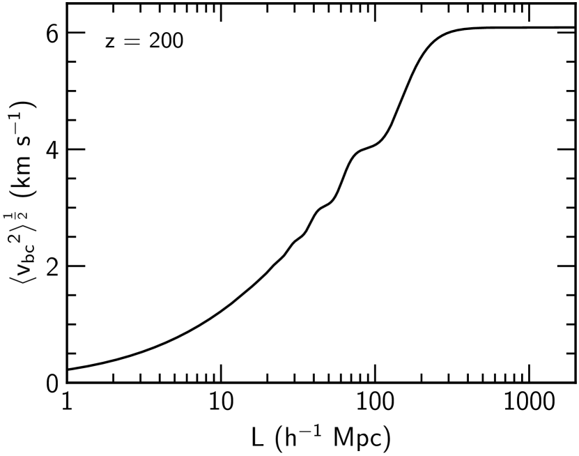
Figure 1: RMS $v_{\rm bc}$ at $z=200$ as a function of box size, calculated by integrating the $v_{\rm bc}$ power spectrum $\Delta_{{v_{\rm bc}}}^{2}$ (computed for the cosmological parameters listed in Section 1) from $2\pi/L$ to $3365~{}h~{}{\rm Mpc^{-1}}$. The RMS $v_{\rm bc}$ converges for $L\gtrsim 400~{}h^{-1}~{}\mathrm{Mpc}$, since $\Delta^{2}_{v_{\rm bc}}$ drops to zero at small-$k$, and so box sizes of this or larger are needed to capture all the relevant scales.

Tseliakhovich & Hirata (2010) showed that most of the contributions to the variance of $v_{\rm bc}$ come from scales between $0.005~{}h~{}{\rm Mpc^{-1}}$ and $0.5~{}h~{}{\rm Mpc^{-1}}$. In a similar fashion to Pontzen et al. (2020), we can compute the RMS $v_{\rm bc}$ inside a box of size $L$ by integrating the power spectrum of $v_{\rm bc}$ fluctuations from the fundamental mode of the box $k_{\rm min}=2\pi/L$ to infinity. The mean square $v_{\rm bc}$ in a box of size $L$ is given by

$$\langle v_{\rm bc}^{2}\rangle_{L}=\int_{2\pi/L}^{k_{\rm max}}{\rm d}k\frac{\Delta_{{v_{\rm bc}}}^{2}}{k},$$ (5)

where $\Delta_{{v_{\rm bc}}}^{2}$ is the dimensionless power spectrum of the $v_{\rm bc}$, taken from camb and, in theory, the upper limit $k_{\rm max}$ of the integral in equation (5) should be the maximum wavenumber of the box, dictated by the number of simulation elements. In practice, however, any upper limit $k_{\rm max}\gg 0.5~{}h~{}{\rm Mpc^{-1}}$ is sufficient, since the $v_{\rm bc}$ power spectrum drops off rapidly above this value. Fig. 1 shows the RMS $v_{\rm bc}$, calculated as the square root of equation (5), where the oscillatory nature of $\Delta_{v_{\rm bc}}^{2}$ at low-$k$ (cf. fig. 1 in Tseliakhovich & Hirata, 2010) is clearly visible. From Fig. 1, we can see that even in a box size of $100~{}h^{-1}~{}\mathrm{Mpc}$, we do not capture all of the scales relevant to $v_{\rm bc}$. The curve only begins to plateau around $\sim 400~{}h^{-1}~{}\mathrm{Mpc}$, so using a box size smaller than this means that we may miss out on some of the effect, for example by not sampling extreme values of $v_{\rm bc}$. Simultaneously simulating this large-scale box and the very high-resolution zoom region needed to observe the effect would be computationally infeasible. In Section 3.2, we discuss our solution to this problem.

3 Methods

3.1 Simulations

We follow the evolution of dark matter, gas, and stars in the cosmological context using ramses, which employs a second-order Godunov method to solve the equations of hydrodynamics. Gas states are computed at cell interfaces using the Harten-Lax-van Leer-contact Riemann solver, with a MinMod slope limiter. Dark matter and stars are modelled as a collisionless $N$-body system, described by the Vlasov-Poisson equations. Grid refinement is performed whenever a cell contains more than eight high-resolution dark matter particles, or has the equivalent amount of baryonic mass scaled by $\Omega_{\rm b}/\Omega_{\rm m}$. We allow the AMR grid to refine from the coarsest level $\ell_{\rm min}=8$ to the finest level $\ell_{\rm max}=23$, but in practice grid hold-back within ramses means that the finest level reached is $\ell=21$, corresponding to a maximum comoving resolution of $47.7~{}h^{-1}~{}\mathrm{pc}$.

Star formation is allowed whenever the gas density of a cell is greater than $n_{\star}=1~{}\mathrm{cm^{-3}}$ in units of the number density of hydrogen atoms and when the local overdensity is greater than $200\rho_{\rm cr}$, where the latter condition prevents spurious star formation at extremely high redshift. We impose a polytropic temperature function with index $g_{\star}=2$ and $T_{0}=1050\,\mathrm{K}$, which ensures that the Jeans length is always resolved by at least eight cells. We do not rigorously calibrate the star formation parameters to reproduce any stellar mass-halo mass relation, since we are interested only in the differences between simulations. Star particles, which represent a population of stars, form with a mass of $108.0~{}h^{-1}~{}\mathrm{M}_{\odot}$. Supernova feedback is included using the kinetic feedback model of Dubois & Teyssier (2008), with a mass fraction $\eta_{\rm SN}=0.1$ and a metal yield of 0.1. We allow gas cooling and follow the advection of metals. We do not include molecular hydrogen in this simulation so, to attempt to compensate for this missing cooling channel, we initialise the zoom region with a metallicity of $Z=10^{-3}~{}{\rm Z_{\odot}}$, where ${\rm Z_{\odot}}=0.02$ in ramses.

3.2 Initial conditions

As described in Section 2, large box sizes of $\ga 400~{}h^{-1}~{}\mathrm{Mpc}$ are required in order to capture all of the scales pertaining to $v_{\rm bc}$. By performing calibration runs, we found that very high resolution (a cell size of $\Delta x\la 2~{}h^{-1}~{}\mathrm{kpc}$) is needed in the ICs in order to properly resolve the effect. To this end, we employ ‘zoom’ initial conditions (ICs), generating density and velocity fields at $z_{\rm ini}=200$ first in a $400~{}h^{-1}~{}\mathrm{Mpc}$ box using music (Hahn & Abel, 2011). The ICs are refined from the base level $\ell_{\rm min}=10$ ($1$,$024^{3}$) up to $\ell=18$ ($262$,$144^{3}$ effective) in a cube of side length $543~{}h^{-1}~{}\mathrm{kpc}$ at the finest level. Such extremely high resolution is required because $v_{\rm bc}$ suppresses structure formation on very small scales. We found that the resolution we used in this work is the minimum necessary to observe the effect of $v_{\rm bc}$, and using lower resolution largely misses the effect. Since the zoom region is very small compared to the box size, we use extra padding between zoom levels, increasing the number of padding cells on each side for each dimension from the typical value of $4$ to $32$. We use transfer functions from camb (Lewis et al., 2000), which gives distinct density and velocity fields for the baryons and dark matter.

Table 1: The sets of ICs used for the main zoom simulation. The columns list the name of each case, which velocity fields are used for the baryons ($\bm{v}_{\rm b}$), whether the baryon fields have been modified and the magnitude of $v_{\rm bc}$ at $z=1000$ ($v_{\rm bc,rec}$), and $z=200$ ($v_{\rm bc,ini}$) in $\mathrm{km}~{}\mathrm{s}^{-1}$. If a value is present for $v_{\rm bc,ini}$, but not $v_{\rm bc,rec}$, then $v_{\rm bc}$ is only included from the start time of the simulation.

Case	$\bm{v}_{\rm b}$	Modified?	$v_{\rm bc,rec}$	$v_{\rm bc,ini}$ ($\mathrm{km}~{}\mathrm{s}^{-1}$)
$\text{no}~{}v_{\rm bc}$	$\bm{v}_{\rm c}$	no	0.0	0.0
$v_{\rm bc}$–ini	$\bm{v}_{\rm b}$	no	0.0	20.09
$v_{\rm bc}$–rec	$\bm{v}_{\rm b}$	yes	100.07	20.09

In order to make the simulation tractable, we extract a $100~{}h^{-1}~{}\mathrm{Mpc}$ ($\ell_{\rm min}=8$, $256^{3}$) base grid from the $400~{}h^{-1}~{}\mathrm{Mpc}$ ($\ell_{\rm min}=10$, $1$,$024^{3}$) box and use this as our coarsest level, meaning that the maximum refinement level in the zoom region also drops two levels from $\ell=18$ to $\ell=16$ ($65$,$536^{3}$ effective). In principle, this methodological choice could introduce some error around the edges of the box due to using periodic boundary conditions with non-periodic ICs, though in practice we expect the impact of this to be negligible since we are concerned with a sub-$h^{-1}~{}\mathrm{Mpc}$ region in the centre of the box. Additionally, these errors will be common between runs, so their effect will wash out when comparing between runs.

Table 1 details the sets of ICs used in this work. We selected a region for zoom-in with $v_{\rm bc,ini}=20.09~{}\mathrm{km}~{}\mathrm{s}^{-1}$ at $z=200$, corresponding to $v_{\rm bc,rec}=100.07~{}\mathrm{km}~{}\mathrm{s}^{-1}$, or $\sim 3.3\sigma_{v_{\rm bc}}$, at recombination. The $\text{no}~{}v_{\rm bc}$ case is often used in cosmological simulations, for example when using transfer functions that do not have separate amplitudes for the baryon and dark matter velocity fields (in fact, it is the default behaviour for older versions of ramses, where the dark matter velocity field is used to initialise both the dark matter and baryon velocities). The $v_{\rm bc}$–ini case is where the simulation is initialised using separate transfer functions for the baryon and dark matter velocity fields, such as by generating ICs using music with transfer functions from camb. In this case, $v_{\rm bc}$ is included from the start time of the simulation $z_{\rm ini}$, but the effect of $v_{\rm bc}$ on density and velocity perturbations between recombination and $z_{\rm ini}$ is missed. In the final, and most realistic, case, $v_{\rm bc}$–rec, we include the contributions from $v_{\rm bc}$ across all $z$ by computing a bias factor which is applied to the ICs. The methodology for computing the bias factor is detailed in Section 3.3.

3.3 Bias factor

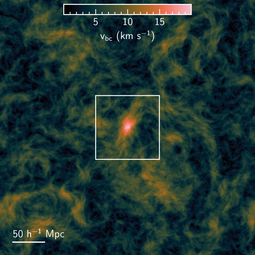
Figure 2: A slice through the large-scale $v_{\rm bc}=|\bm{v}_{\rm b}-\bm{v}_{\rm c}|$ field in the full $400~{}h^{-1}~{}\mathrm{Mpc}$ initial conditions at $z_{\rm ini}=200$. Each pixel corresponds to a cell width of $0.39~{}h^{-1}~{}\mathrm{Mpc}$ and the slice has a thickness of one cell width. Also shown (white square) is the position of the extracted $100~{}h^{-1}~{}\mathrm{Mpc}$ subbox, centred on the peak $v_{\rm bc}$ in the ICs. The zoom region is located in the centre of the subbox. The colour shows the magnitude of the $v_{\rm bc}$ at $z_{\rm ini}=200$, where light pink is high $v_{\rm bc}$ and dark blue is low $v_{\rm bc}$.

Using transfer functions that have distinct amplitudes for the baryon and dark matter velocity fluctuations naturally yields the $v_{\rm bc}$ field at the start time of the simulation $z_{\rm ini}$. First, we interpolate the dark matter particle velocities onto the same grid as the baryons, then take the difference of these two fields to calculate the magnitude as $v_{\rm bc}=\left|\bm{v}_{\rm b}-\bm{v}_{\rm c}\right|$. A $0.39~{}h^{-1}~{}\mathrm{Mpc}$ thick slice through the resultant $v_{\rm bc}$ field is shown in Fig. 2.

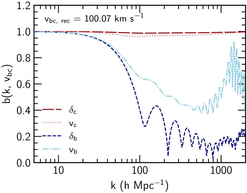
Figure 3: The bias factors $b(k\,v_{\rm bc})$ at $z_{\rm ini}=200$ for the average $v_{\rm bc}$ in the zoom region, scaled back to its value at recombination $v_{\rm bc,rec}=100.07~{}\mathrm{km}~{}\mathrm{s}^{-1}$, which is a $\sim 3.3\sigma_{v_{\rm bc}}$ value. We show $b(k,v_{\rm bc})$ for baryon and dark matter overdensities and peculiar velocities. These are the bias factors that are applied to the perturbations in the zoom region. Note how the perturbations in the baryon overdensity (dark blue, short-dashed) are strongly suppressed for $k>40~{}h~{}\mathrm{Mpc}^{-1}$, while the perturbations in the dark matter overdensity (dark red, long-dashed) are largely unaffected, to the few per cent level. Note that we show $b(k,v_{\rm bc})$ for the peculiar velocities for the full range of $k$, but the velocity field is dominated by large-scale (small-$k$) modes. Therefore, $b(k,v_{\rm bc})$ will have little if any impact on the small scales (large-$k$) of the velocity field.

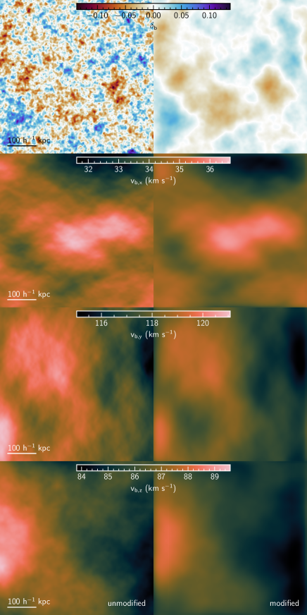
Figure 4: Slices of the unmodified (left column) and modified (through convolution with the bias factor, as in equation (7), right column) baryon overdensity (top row), peculiar velocity in the $x$-direction (second row), $y$-direction (third row) and $z$-direction (bottom row) in the high-resolution zoom region, of side length $543~{}h^{-1}~{}\mathrm{kpc}$. Each pixel corresponds to a cell width of $1.53~{}h^{-1}~{}\mathrm{kpc}$ and the slice has a thickness of one cell width. The effect of applying $b(k,v_{\rm bc})$, defined in equation (6), can be clearly seen in the baryon overdensity, in that it washes out the small-scale fluctuations. The effect is less pronounced in the peculiar velocities, which are dominated by large-scale modes.

With the $v_{\rm bc}$ field in hand, we split our ICs into cubic patches, aiming for a patch extent of $0.5~{}h^{-1}~{}\mathrm{Mpc}$, though the actual extent depends upon how many patches can be fit in each level of the grafic files. The size of these patches is chosen to be smaller than the scale over which $v_{\rm bc}$ is coherent (Tseliakhovich & Hirata, 2010). Within each patch, the average value of $v_{\rm bc}$ is calculated and used as $v_{\rm bc}$ in equations (2). The initial values for equations (2) are set using the transfer functions from camb at $z=1000$, and the equations are integrated from $z=1000$ to $z=200$ using the lsoda ordinary differential equation solver. Equations (2) are solved for the average patch value of $v_{\rm bc}$ and also for $v_{\rm bc}=0~{}\mathrm{km}~{}\mathrm{s}^{-1}$, which yields power spectra for the baryon perturbations both with and without $v_{\rm bc}$. We use these power spectra to calculate a ‘bias’ factor at $z_{\rm ini}=200$ that depends both upon scale $k$ and the magnitude of the relative velocity $v_{\rm bc}$

$$b(k,v_{\rm bc})=\left[\frac{P(k,v_{\rm bc})}{P(k,v_{\rm bc}=0)}\right]^{\frac{1}{2}},$$ (6)

where the square root arises from $P\propto\left|\delta^{2}\right|$. In Fig. 3, we show the bias factor for the baryon and dark matter densities ($\delta_{\rm b}$ and $\delta_{\rm c}$) and velocities ($v_{\rm b}$ and $v_{\rm c}$), computed for the average $v_{\rm bc}$ in our zoom region. The strongest suppression is seen in the baryons and in particular the baryon density, while the dark matter is hardly affected. We do not expect the oscillatory features in $b(k,v_{\rm bc})$ at the very small scales to have much, if any, impact since the power spectrum of fluctuations in the baryon density contrast begins to fall rapidly for $k\gtrsim 300~{}h~{}\mathrm{Mpc}^{-1}$, while for the velocity most of the power is at much larger scales. Ali-Haïmoud et al. (2014) also found oscillatory features in the small-scale baryon perturbations, and we have checked that we find similar oscillations for typical values of $v_{\rm bc}$ and also find that increasing the magnitude of $v_{\rm bc}$ increases the frequency of oscillations for the larger-scale ($\gtrsim 100~{}h~{}\mathrm{Mpc}^{-1}$) modes too. For a detailed study into the origin of these small-scale oscillations, we defer the reader to Ali-Haïmoud et al. (2014). This factor is then convolved with the Fourier transform of the corresponding patch of baryon overdensity

$$\hat{\delta}_{\rm b}(k,v_{\rm bc})=b(k,v_{\rm bc})\cdot\delta_{\rm b}(k)$$ (7)

to give individual patches of biased overdensity $\hat{\delta}_{\rm b}$, which are then stitched together to generate the $v_{\rm bc}$–rec set of ICs. In this way, the bias factor compensates for the suppression of baryon perturbations between $z=1000$ and $z_{\rm ini}$ that is missing if $v_{\rm bc}$ is included only from $z_{\rm ini}$. We only modify the baryons, since as discussed earlier, they are much more strongly affected than the dark matter, as can be seen from Fig. 3.

We deal with the peculiar velocity field for the baryons in a similar way, by first converting the velocity divergence to peculiar velocities as $\bm{v}_{\rm b}(k)=-{\rm i}a\bm{k}\theta_{\rm b}(k)/k^{2}$. Note again that we do not include directionality when solving the evolution equations, and therefore, the bias factor is applied to each direction of $\bm{v}_{\rm b}$ equally. In reality, there would be preferential directions for the bias factor, depending on the direction of $\bm{v}_{\rm bc}$, but we defer that implementation to future work.

Fig. 4 shows a $1.53~{}h^{-1}~{}\mathrm{kpc}$ thick slice through the highest resolution level of the zoom ICs directly from music (‘unmodified’, left column) and after the bias factor $b(k,v_{\rm bc})$ has been applied (‘modified’, right column). For $\delta_{\rm b}$ (top row), the unmodified ICs contain a lot of small-scale structure, which is almost totally washed out after applying $b(k,v_{\rm bc})$. Most of what remains is in the form of lower amplitude, larger scale fluctuations. For $v_{{\rm b},i}$ (bottom rows), there is less small-scale structure to begin with, since the peculiar velocity fields are dominated by large scales. The effect of $b(k,v_{\rm bc})$ on $v_{{\rm b},i}$ is therefore much less striking than on the $\delta_{\rm b}$, with the main effect being smoothing and a slight reduction in amplitude.

3.4 Haloes

After the ICs have been correctly initialised with $v_{\rm bc}$, we can characterise the effect of $v_{\rm bc}$ on structure formation, principally by exploring how haloes are affected. Haloes are identified using ahf (Gill et al., 2004; Knollmann & Knebe, 2009), which supports multi-resolution datasets and calculates baryonic properties of haloes. In order to use ahf with a ramses dataset, we use the supplied ramses2gadget tool to convert leaf cells of the AMR hierarchy into gas pseudoparticles placed at the centre of each cell. This conversion is a standard recipe in the analysis of AMR datasets (e.g. Wu et al., 2015) and allows us to conveniently assign gas to haloes. We ignore the internal energy of the gas and do not allow ahf to perform any unbinding, as this has been shown to remove most of the gas from subhaloes in a manner that is dependent upon the choice of halo finder (Knebe et al., 2013). We define the halo overdensity with respect to the critical density $\rho_{\rm cr}$, such that the average density inside the halo is $200\rho_{\rm cr}$.

Guided by the resolution study of Naoz & Barkana (2007), we perform our analysis on haloes that have $\geq 500$ particles, as they found that this is the level at which the baryon fraction is resolved with a scatter of $\sim 20~{}{\rm per~{}cent}$ when compared to higher resolution simulations.

We only use haloes comprised entirely of high-resolution dark matter particles, since contaminant low-resolution particles can disrupt the dynamics of haloes (Oñorbe et al., 2014). Due to the small size of the zoom region, it is often the case that haloes which were initially solely composed of high-resolution particles can become contaminated by low-resolution particles as the simulation progresses. If contaminated haloes are removed at each timestep, then haloes can ‘disappear’ if they become contaminated between one timestep and the next. To counter this effect, we generate merger trees using consistent-trees (Behroozi et al., 2013) and only keep haloes that have never been contaminated at any point in the simulation. Then, when exploring the effect on halo properties (such as when looking at their gas content), we go one step further and match haloes between the simulations. We do this using ahf’s MergerTree tool to correlate the particle IDs between each run. This allows us to isolate the effect on identical haloes, as opposed to also capturing the impact on the global population of haloes. The difficulties in exploring the impact on the global population of haloes (e.g. through the cumulative number of haloes) are explored in Section 4.1.

4 Results

4.1 Halo abundances

Throughout this section, we calculate the cumulative number of haloes $N(>M)$ as the number of haloes with a total mass greater than $M$ and estimate the Poisson uncertainty on $N(>M)$ for each case as $\sqrt{N(>M)}$. To begin with, we ignore the conditions described in Section 3.4, instead considering the cumulative number of all haloes formed in the simulation $N_{\rm all}(>M)$, shown in Fig. 5. Aside from a slight suppression in $N_{\rm all}(>M)$ for the $v_{\rm bc}$–rec case below $10^{6}~{}h^{-1}~{}\mathrm{M}_{\odot}$ at $z=14.2$, the $v_{\rm bc}$–ini and $v_{\rm bc}$–rec cases are consistent both with each other and with the $\text{no}~{}v_{\rm bc}$ case at the $1\sigma$ level. Analysing the haloes in this fashion (i.e. by performing no cleaning on the catalogue) gives a picture of the global impact of $v_{\rm bc}$ on halo abundance, however this picture is inaccurate because a significant fraction of the haloes are contaminated by, or formed entirely of, lower-resolution particles, affecting the accuracy of their properties (see Section 3.4 for a discussion of contamination).

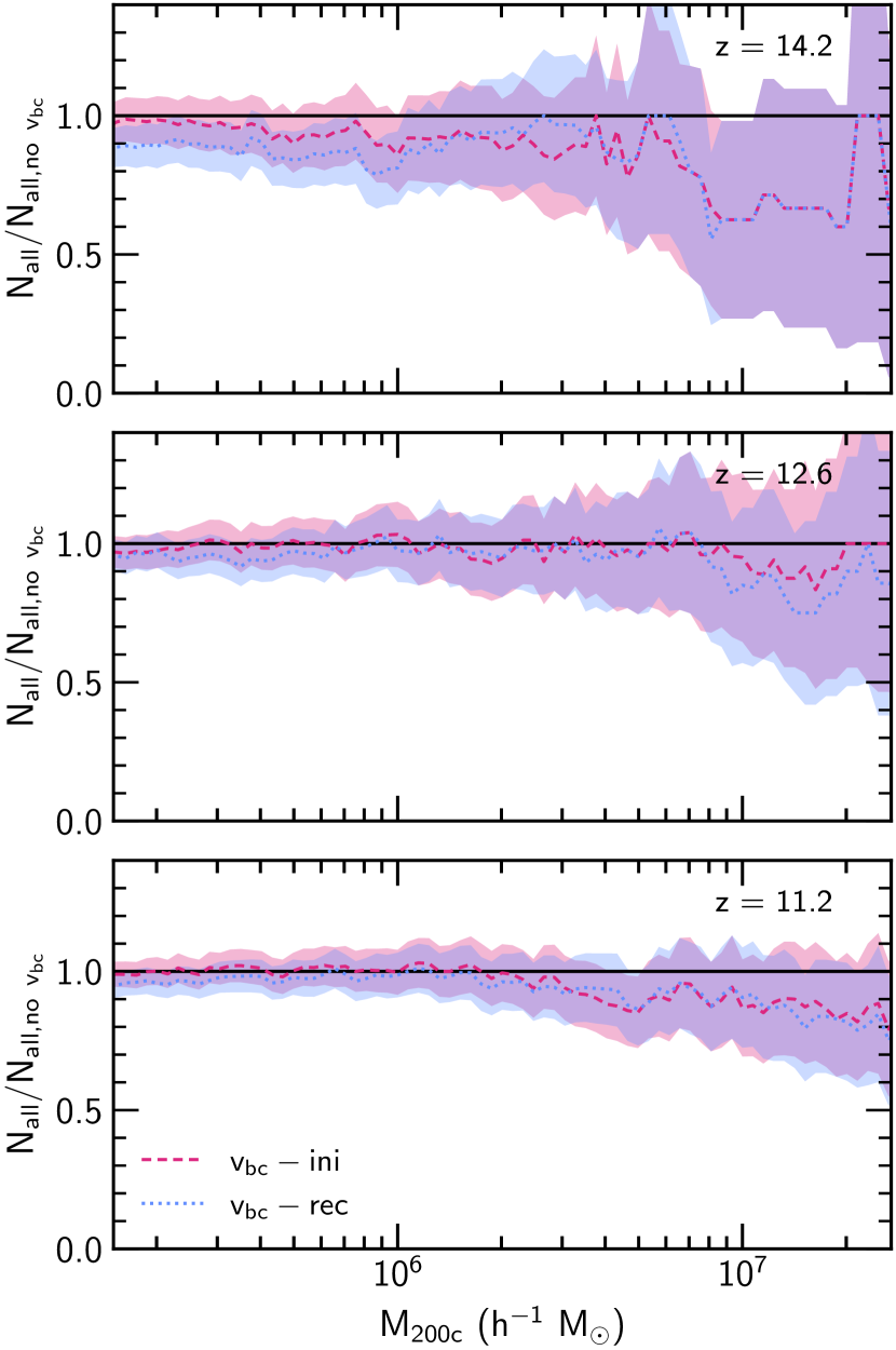
Figure 5: Ratio of the cumulative number of haloes $N_{\rm all}(>M)$ in the $v_{\rm bc}$–ini (pink short-dashed) and the $v_{\rm bc}$–rec (blue dotted) cases to the $\text{no}~{}v_{\rm bc}$ case at $z=14.2$ (top), $12.6$ (middle), and $11.2$ (bottom). All the haloes found by ahf are included in $N_{\rm all}(>M)$. The shaded regions indicate the $1\sigma$ Poisson uncertainty on the ratio. $N_{\rm all}(>M)$ is broadly the same between all three sets of simulations, except for a suppression in the number of haloes with $M<10^{6}~{}h^{-1}~{}\mathrm{M}_{\odot}$ at $z=14.2$ in the $v_{\rm bc}$–rec case compared to the $\text{no}~{}v_{\rm bc}$ case.

If we now apply the conditions described in Section 3.4, namely that we do not include in our analysis any haloes that are contaminated at any point in the simulation, we are left with a reduced catalogue. In Fig. 6, we show the cumulative number of haloes in this cleaned catalogue $N_{\rm clean}(>M)$, which shows a much more striking suppression of $N_{\rm clean}(>M)$ for the $v_{\rm bc}$–rec case and an apparent increase in the abundance of low-mass ($M<10^{6}~{}h^{-1}~{}\mathrm{M}_{\odot}$) haloes for the $v_{\rm bc}$–ini case at $z=11.2$ (though still consistent with no difference to the $\text{no}~{}v_{\rm bc}$ case at the $1\sigma$ level).

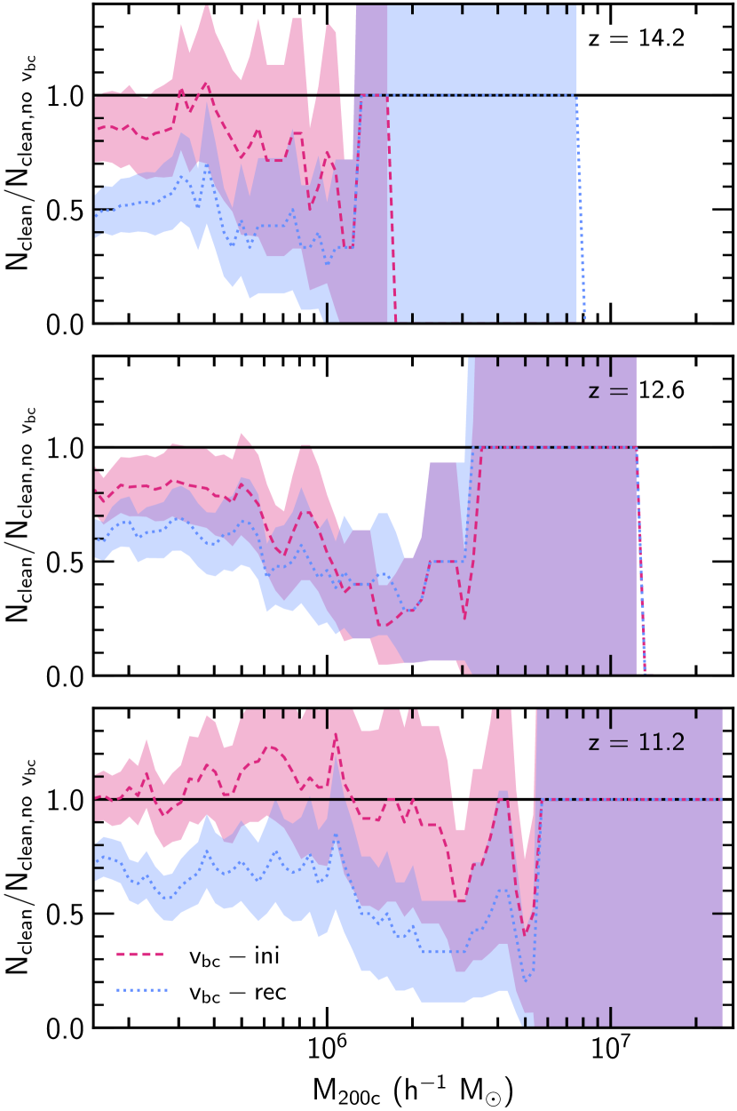
Figure 6: As in Fig. 5, but this time $N_{\rm clean}(>M)$ includes only haloes that have been selected by the process detailed in Section 3.4. Selecting never-contaminated haloes in this fashion leads to the removal of an unequal and inconsistent number of haloes between each run—this leads to the odd behaviour of the $v_{\rm bc}$–ini curve, which jumps from a suppression to a boost in the number of haloes with $M<2\times 10^{6}~{}h^{-1}~{}\mathrm{M}_{\odot}$ between $z=12.6$ and $11.2$.

To highlight the effect of the cleaning procedure we also show the raw cumulative number of haloes at $z=14.2$ and $z=11.2$ in Fig. 7. The impact of the cleaning process described in Section 3.4 can be clearly seen in the bottom panel of Fig. 7, which shows the ratio of the cleaned catalogue to the full catalogue $N_{\rm clean}(>M)/N_{\rm all}(>M)$. Comparing the different runs, it can be clearly seen that a different fraction of haloes is removed between each run at each of the times shown.

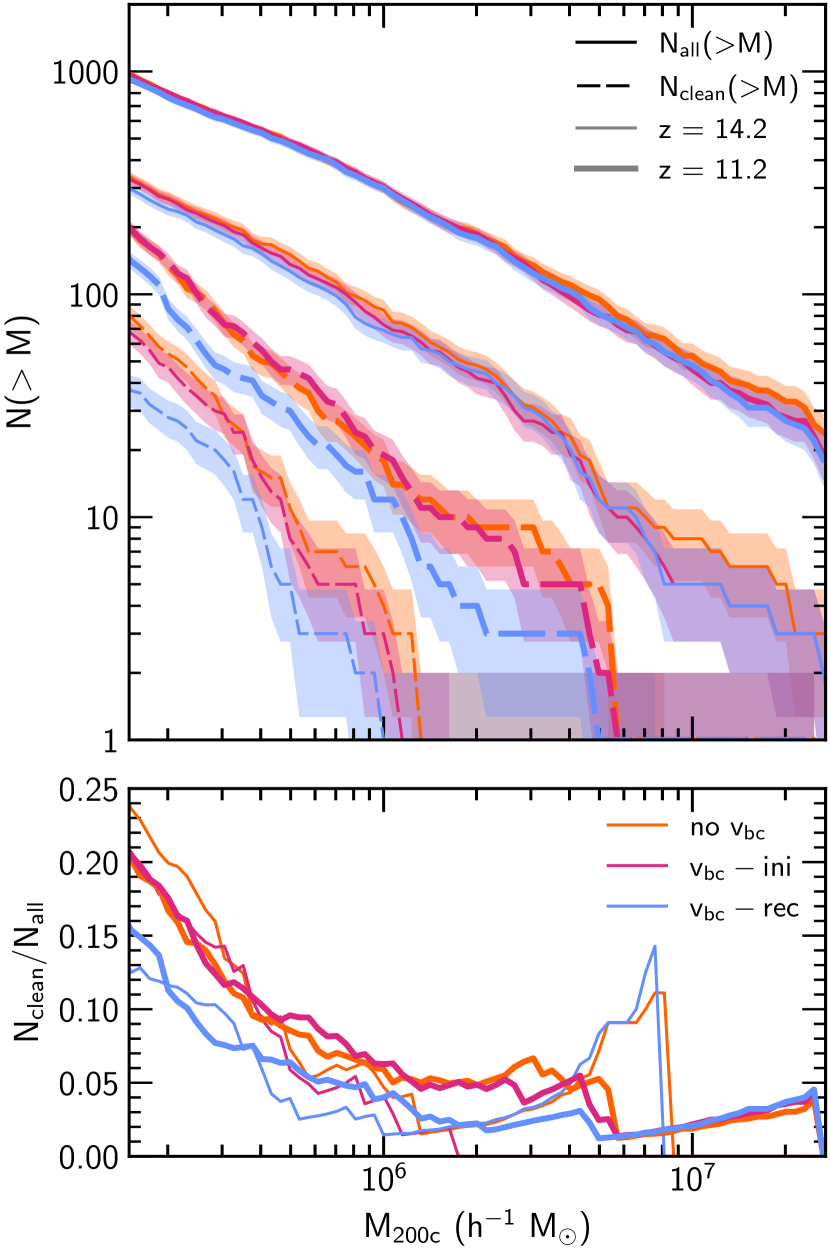
Figure 7: Cumulative number of haloes (top panel) for the raw catalogue $N_{\rm all}(>M)$ (solid) and the catalogue cleaned according to the prescription in Section 3.4 $N_{\rm clean}(>M)$ (long-dashed) and the ratio of $N_{\rm clean}(>M)$ to $N_{\rm all}(>M)$ (bottom panel) at each $z$. We show $N(>M)$ at $z=14.2$ (thin) and $11.2$ (thick). From the top panel, it can be seen that $N_{\rm all}(>M)$ is very similar between all runs at each $z$ shown, except for a slight suppression in the abundance of haloes in the $v_{\rm bc}$–rec case at $z=14.2$. The huge reduction in the number of haloes after cleaning the catalogue is abundantly clear, as is the difference in fraction of haloes removed between each run.

4.2 Baryon fraction

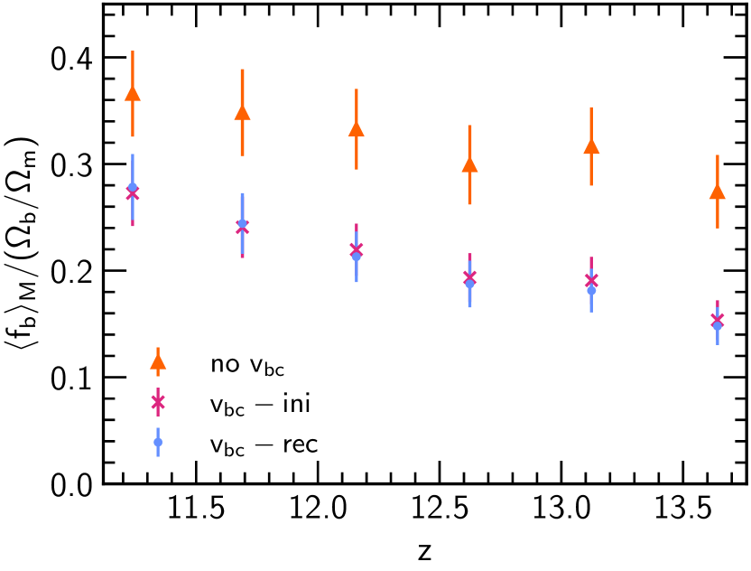
Figure 8: Mass-weighted average baryon fraction $f_{\rm b}$ as a function of redshift $z$, normalised to the cosmic mean $\Omega_{\rm b}/\Omega_{\rm m}$. The average is shown for all $z$ where more than $30$ haloes have formed. The errorbars show the $1\sigma$ standard deviation as calculated using equation (10). We find a suppression in both the $v_{\rm bc}$–ini and $v_{\rm bc}$–rec cases compared to the $\text{no}~{}v_{\rm bc}$ run, though between the two runs with $v_{\rm bc}$ there is little difference.

We allow star formation in these runs, so the total baryon fraction of a given halo is defined as

$$f_{\rm b}=\frac{M_{\rm g}+M_{\star}}{M_{\rm d}+M_{\rm g}+M_{\star}},$$ (8)

where $M_{\rm g}$ is the gas, $M_{\star}$ the stellar, and $M_{\rm d}$ the dark matter mass in each halo. We upweight the best resolved (i.e. most massive) haloes by calculating the mass-weighted average baryon fraction as

$$\langle f_{\rm b}\rangle_{M}=\frac{\sum_{i}f_{{\rm b},i}M_{i}}{\sum_{i}M_{i}}$$ (9)

and the associated mass-weighted standard deviation as

$$\sigma_{M}=\left(\frac{\sum_{i}f^{2}_{{\rm b},i}M_{i}}{\sum_{i}M_{i}}-\langle f_{\rm b}\rangle_{M}^{2}\right)^{\frac{1}{2}},$$ (10)

where the sum is over all haloes that satisfy the conditions in Section 3.4. Fig. 8 shows $\langle f_{\rm b}\rangle_{M}$ and associated $1\sigma$ errorbars as function of $z$. We show each $z$ where $\geq 30$ haloes have formed that satisfy the criteria in Section 3.4, starting from $z=13.6$ where we are able to match $38$ haloes between the three cases. The gas fraction is suppressed at all $z$ for the $v_{\rm bc}$–ini and $v_{\rm bc}$–rec cases compared to the $\text{no}~{}v_{\rm bc}$ case. At earlier $z$, the suppression is stronger, though even by the final snapshot at $z=11.2$, $\langle f_{\rm b}\rangle_{M}$ for both the $v_{\rm bc}$–rec and $v_{\rm bc}$–ini cases are not within $1\sigma$ of the $\text{no}~{}v_{\rm bc}$ case. Notably, at all $z$, $\langle f_{\rm b}\rangle_{M}$ in $v_{\rm bc}$–ini and $v_{\rm bc}$–rec cases are almost indistinguishable from, and certainly consistent with, one another.

4.3 Star formation

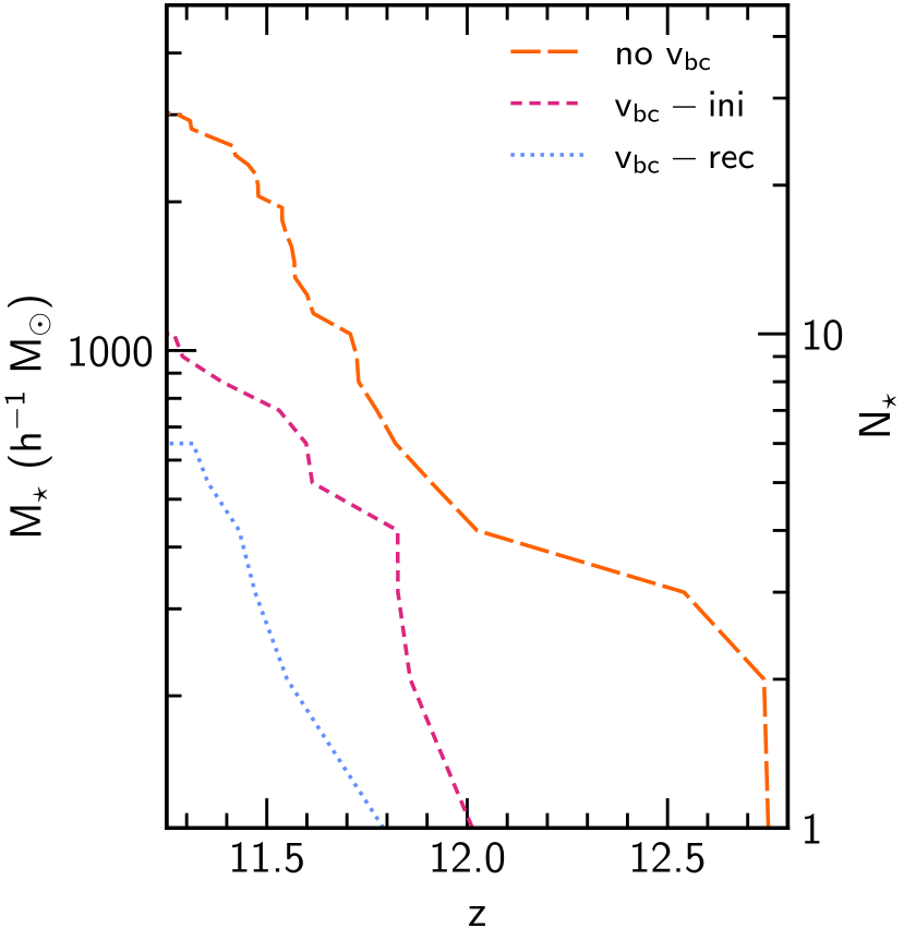
Figure 9: Cumulative stellar mass $M_{\star}$ formed as function of redshift $z$. Also shown is the corresponding number of stellar particles $N_{\star}$. Despite the small number of stars formed in this simulation, there is a clear hierarchy in how many stars each forms, with the $\text{no}~{}v_{\rm bc}$ run forming the most, followed by $v_{\rm bc}$–ini and then $v_{\rm bc}$–rec. There is also a clear delay in the onset of star formation which follows a similar trend, with the $v_{\rm bc}$–rec run starting to form stars the latest.

In Fig. 9, we show the cumulative $M_{\star}$ formed in the simulation, not accounting for mass loss due to supernovae, and the corresponding number of stellar particles $N_{\star}$, which each have a mass of $108.0~{}h^{-1}~{}\mathrm{M}_{\odot}$. In each case, all of the star particles in the simulation formed inside a single halo. In total, $29$ star particles formed by $z=11.2$ in the $\text{no}~{}v_{\rm bc}$ case, $10$ in the $v_{\rm bc}$–ini case, and $7$ in the $v_{\rm bc}$–rec case. This hierarchy persists across all $z$, with more star particles having formed in the $\text{no}~{}v_{\rm bc}$ case than in the $v_{\rm bc}$–ini case and fewer still in the $v_{\rm bc}$–rec case.

In the following, all times quoted in $\mathrm{Myr}$ are measured relative to the Big Bang. To quantify how $v_{\rm bc}$ impacts star formation in our simulations, we can calculate the delay in formation time of the $n$th star $t_{n}$ for each run with $v_{\rm bc}$ compared to the $\text{no}~{}v_{\rm bc}$ run $t_{n,\,\text{no}~{}v_{\rm bc}}$ as $\Delta t_{n}=t_{n}-t_{n,\,\text{no}~{}v_{\rm bc}}$. For the $v_{\rm bc}$–ini case, the smallest (largest) delay of $8.6~{}\mathrm{Myr}$ ($35.5~{}\mathrm{Myr}$) occurs for the formation of the fourth (second) star particle, while for the $v_{\rm bc}$–rec case we find a delay of $23.4~{}\mathrm{Myr}$ ($49.4~{}\mathrm{Myr}$) for the sixth (second) star particle to form.

Star formation in ramses (like in other simulation codes) is a stochastic process, hence the large fluctuations in delay times. We can reduce the impact this stochasticity has on our results by averaging over delay times, as opposed to considering the delay times for individual star particles. We find a mean delay time of $\langle\Delta t\rangle=19.4~{}\mathrm{Myr}$ and $34.9~{}\mathrm{Myr}$ for the $v_{\rm bc}$–ini and $v_{\rm bc}$–rec cases, respectively.

5 Discussion

To understand the perceived uptick in $v_{\rm bc}$–ini haloes in Fig. 6, we need to explore the raw cumulative number of haloes, shown in Fig. 7 at $z=14.2$ and $z=11.2$. The key point is that while only keeping haloes that are never contaminated ensures that haloes do not disappear between timesteps of the same run, it also means that different numbers of haloes will be removed between different runs at any given timestep. This discrepancy in the number of haloes removed is responsible for the apparent low-mass boost in the $v_{\rm bc}$–ini case, because over the mass range $3\times 10^{5}<M/h^{-1}~{}\mathrm{M}_{\odot}<10^{6}$ fewer haloes are removed in the $v_{\rm bc}$–ini case than in the $\text{no}~{}v_{\rm bc}$ case. Since the cumulative numbers of haloes are already very similar, removing a smaller number of haloes in the $v_{\rm bc}$–ini case manifests itself as a boost relative to the $\text{no}~{}v_{\rm bc}$ case, when in fact it is simply an artefact of the cleaning procedure.

Given the difficulties in extracting a sample of haloes that is both free from contamination and comparable between runs, we will not draw any quantitative conclusions on the impact of $v_{\rm bc}$ on global properties like the number of haloes formed. We retain this discussion of the well-known impact of contamination and, crucially, the importance of verifying any mitigation techniques as it may prove helpful for other works employing zoom simulations.

Including $v_{\rm bc}$ also significantly affects the baryon fraction $f_{\rm b}$, where we see that the mass-weighted baryon fraction $\langle f_{\rm b}\rangle_{M}$ is suppressed at all redshifts in both cases, with the suppression stronger at higher redshift. Even by $z=11.2$, the $v_{\rm bc}$–ini and $v_{\rm bc}$–rec cases are still not in agreement with the $\text{no}~{}v_{\rm bc}$ case, though the difference between the two populations has decreased. Again, this is likely due to the decay in the magnitude of $v_{\rm bc}$, which allows the haloes to accrete more gas. Interestingly, $\langle f_{\rm b}\rangle_{M}$ is almost indistinguishable between the $v_{\rm bc}$–ini and $v_{\rm bc}$–rec cases, suggesting that including $v_{\rm bc}$ from $z_{\rm ini}$ is sufficient to observe its impact on halo baryon fraction, though a larger sample is required to confirm this. The suppression in $\langle f_{\rm b}\rangle_{M}$ when $v_{\rm bc}$ is included is in qualitative agreement with previous studies.

This decrement in baryon fraction for the $v_{\rm bc}$–ini and $v_{\rm bc}$–rec cases is reflected in the cumulative stellar mass formed, as fewer star particles formed in both cases than in the $\text{no}~{}v_{\rm bc}$ case. Not only do they form fewer star particles, they also start forming star particles later since the effect of $v_{\rm bc}$ is to wash out the peaks (and troughs) in the baryon density contrast, meaning that it takes longer for gas to reach the densities required for star formation. The mean delay for forming star particles is $19.4~{}\mathrm{Myr}$ for the $v_{\rm bc}$–ini case and $34.9~{}\mathrm{Myr}$ for the $v_{\rm bc}$–rec case. From Schaerer (2002), we find that these delays are all of the order of the lifetime of a $9~{}\mathrm{M}_{\odot}$ first-generation Population (Pop) III star, which has a lifetime of $20.02~{}\mathrm{Myr}$ (table 3 in Schaerer, 2002). More massive Pop III stars have even shorter lifetimes, for example a $120~{}\mathrm{M}_{\odot}$ Pop III star lives for only $2.52~{}\mathrm{Myr}$. Pop III stars form from initially pristine gas, and their death pollutes their immediate surroundings with metals, introducing new cooling channels into the high-redshift Universe. Any delay in this introduction of metals will delay the transition between Pop III to Pop II (i.e. from metal-enriched gas), which can, for example, affect the $21~{}{\rm cm}$ signal (Magg et al., 2022). In our case, though we do not form Pop III stars, chemical enrichment is still vitally important for star formation to get properly underway, particularly as all of the star particles form in the same halo.

Despite there being almost no difference in $\langle f_{\rm b}\rangle_{M}$ between the $v_{\rm bc}$–ini and $v_{\rm bc}$–rec cases at most redshifts, there is a clear hierarchy in the amount of stars formed—$\text{no}~{}v_{\rm bc}$ forms the most, $v_{\rm bc}$–ini forms fewer, and $v_{\rm bc}$–rec forms the least—albeit on the order of a few star particles. This effect is expected, since the bias factor washes out baryonic density peaks, and there are slightly more haloes (i.e. star formation locations) present in the $v_{\rm bc}$–ini case than in the $v_{\rm bc}$–rec case.

6 Conclusions

We have performed the first cosmological zoom simulations that self-consistently sample the relative baryon-dark matter velocity $v_{\rm bc}$ from a large $400~{}h^{-1}~{}\mathrm{Mpc}$ box. This relative velocity naturally arises when simulations are initialised using transfer functions that have separate amplitudes for the baryon and dark matter velocities, and we have shown that a box roughly as large as this is required to properly sample all of the scales associated with the relative velocity. However, solely initialising simulations in this manner misses out on the effect of the relative velocities from $z=1000$ to the start time of the simulation, $z_{\rm ini}$. We developed a methodology that compensates for the effect of $v_{\rm bc}$ on baryon density and velocity perturbations by computing a ‘bias’ factor $b(k,v_{\rm bc})$, which is convolved with the ICs. We verified that our methodology performs as expected by comparing to previous works (see Appendix A).

As a first demonstration of our methodology, we applied it to an extremely high-resolution zoom region in a $100~{}h^{-1}~{}\mathrm{Mpc}$ subbox, extracted from the main $400~{}h^{-1}~{}\mathrm{Mpc}$ box. The zoom region is centred on the region with the largest relative velocity in the $400~{}h^{-1}~{}\mathrm{Mpc}$ box, which has an RMS value of $v_{\rm bc}=100.07~{}\mathrm{km}~{}\mathrm{s}^{-1}$ at $z=1000$, corresponding to $\sim 3.3\sigma_{v_{\rm bc}}$. We find qualitative agreement with previous works, namely a reduction in the halo baryon fraction, a delay in the onset of star formation at high redshift, and a suppression of the final stellar mass. The strength of the effect decreases with redshift, but the two simulations still exhibit some differences by $z=11.2$. We find that the delay in the onset of star formation is of the order of the lifetime of a $\sim 9~{}\mathrm{M}_{\odot}$ Pop III star. We also test the effect of incorporating the bias factor by running a simulation that includes the relative velocity from the start time of the simulation only. In this case, we find that more stars are formed when compared to the simulation that includes the bias factor, but there is almost no change in the average baryon fraction, except at the earliest redshift. Due to the small size of our zoom region, the vast majority of haloes in our simulation are contaminated with low-resolution particles, and we are thus unable to draw any robust conclusions regarding the halo mass function.

Our code for producing these compensated ICs is publicly available, and we hope will be of use for studying this effect in the full cosmological context.

Data Availability

The code for computing and applying the bias factor $b(k,v_{\rm bc})$ is available at https://github.com/lconaboy/drft. The data underlying this article will be shared on reasonable request to the corresponding author.

Appendix A Comparison to previous works

We run a series of test simulations set up as in Naoz et al. (2012, 2013). The specific case shown here has a base resolution $\ell_{\rm min}=9$ ($512^{3}$ dark matter particles and, initially, cells), in a $471.1~{}h^{-1}~{}\mathrm{kpc}$ periodic box. The simulations in Naoz et al. (2012, 2013) were performed using the SPH code gadget2 (Springel, 2005), while we use the AMR code ramses. We allow the AMR grid to refine freely up to $\ell_{\rm max}=14$, corresponding to a maximum comoving resolution of $28.9~{}h^{-1}~{}\mathrm{pc}$, comparable to the gravitational softening length of $45.8~{}h^{-1}~{}\mathrm{pc}$ comoving used in Naoz et al. (2012). We use our fiducial cosmology (Section 3.1), whereas Naoz et al. (2012) used a cosmology consistent with Komatsu et al. (2009) with parameters: $\Omega_{\rm m}=0.28$, $\Omega_{\Lambda}=0.72$, $\Omega_{\rm b}=0.046$, $h=0.7$ and a boosted $\sigma_{8}=1.4$. We adopt the boosted $\sigma_{8}=1.4$ as used in the original studies. We initialise the simulations at $z_{\rm ini}=200$ both with and without a relative velocity of $1.7\sigma_{v_{\rm bc}}=10~{}\text{km~{}s}^{-1}$ at $z_{\rm ini}$. We also compute and apply the bias factor $b(k,v_{\rm bc})$ to the baryonic component of the ICs, while the Naoz et al. (2012) simulations are initialised by computing transfer functions which explicitly include the effect of the $v_{\rm bc}$. Following Naoz et al. (2012), we set both of the velocity fields to that of the dark matter and apply the $v_{\rm bc}$ to the $x$-component of the baryon velocity as

$$\begin{pmatrix}v_{\mathrm{b},x}\\ v_{\mathrm{b},y}\\ v_{\mathrm{b},z}\end{pmatrix}=\begin{pmatrix}v_{\mathrm{c},x}+v_{\rm bc}\\ v_{\mathrm{c},y}\\ v_{\mathrm{c},z}\end{pmatrix}.$$ (11)

Including the $v_{\rm bc}$ in this manner is justified by the box size being much smaller than the coherence scale of the $v_{\rm bc}$. We do not allow star formation in these runs. Haloes are identified as described in Section 3.4, noting that although Naoz et al. (2012) define their halo overdensity with respect to the background matter density $\bar{\rho}_{\rm m}$, we are working in the period of matter domination so the difference will be small. While the final halo masses in Naoz et al. (2012) are defined using a spherical overdensity method, the initial halo finding is done using a friend-of-friends method, which could be susceptible to ‘overlinking’ (e.g. Davis et al., 1985), whereby disparate groups of particles are spuriously connected by a diffuse particle bridge. Their redefinition of the halo mass using the spherical overdensity method will go some way to alleviating the impact (if any) of overlinking.

To calculate the effect of the $v_{\rm bc}$, we compare to simulations without $v_{\rm bc}$, where the velocity field of the baryons is equal to that of the dark matter. In order to quantify this effect, we calculate the fractional difference of a quantity $A$ as

$$\Delta_{A}=\frac{A_{v_{\rm bc}}-A_{{\rm no}~{}v_{\rm bc}}}{A_{{\rm no}~{}v_{\rm bc}}}.$$ (12)

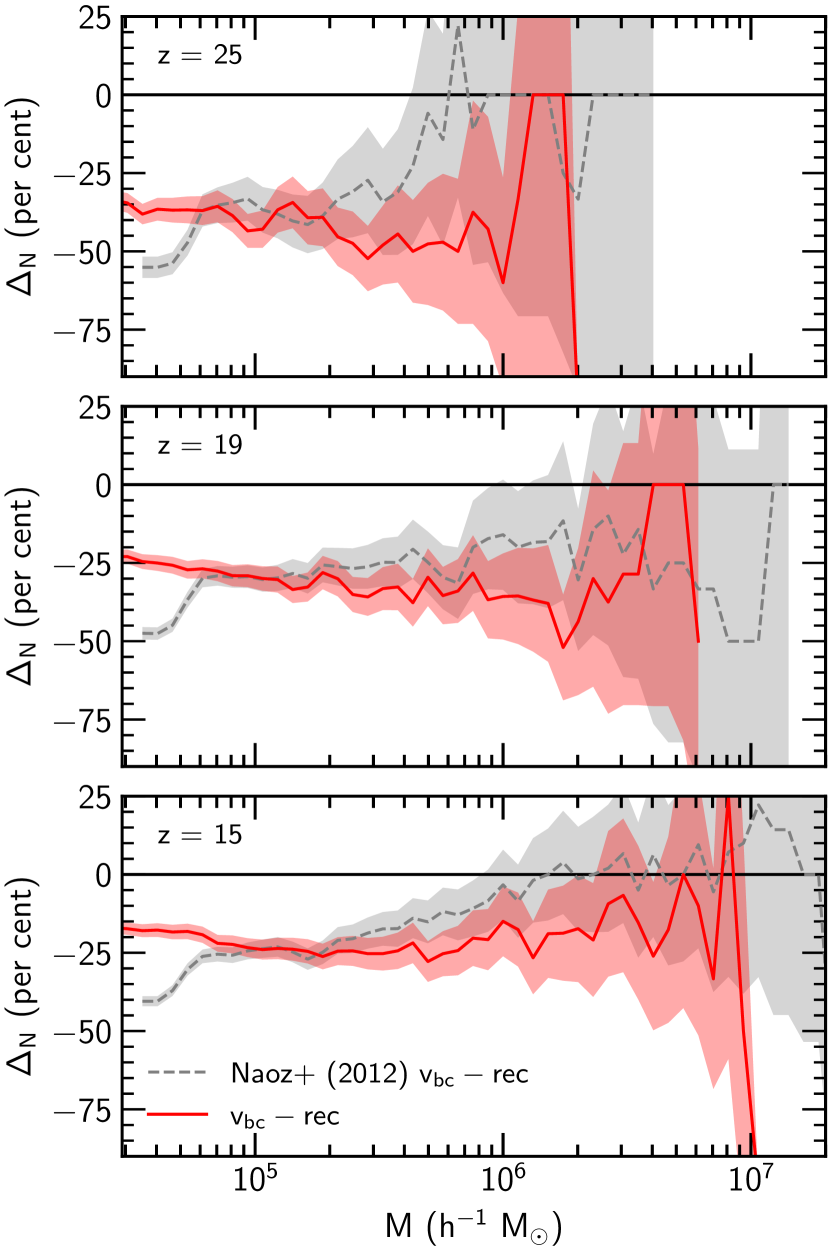
Figure 10: The fractional difference $\Delta_{N}$ in halo mass function $N(>M)$ for the $v_{\rm bc,ini}=10~{}\mathrm{km}~{}\mathrm{s}^{-1}$ case, calculated with equation (12). We show $\Delta_{N}$ at $z=25$ (top), $19$ (centre), and $z=15$ (bottom) for our simulations (red solid) and for the Naoz et al. (2012) work (grey dashed). The shaded regions indicate the $1\sigma$ Poisson uncertainty on the ratio. At most masses we are consistent with Naoz et al. (2012), though there is some disagreement for $M<6\times 10^{4}~{}h^{-1}~{}\mathrm{M}_{\odot}$, which could arise because of the friends-of-friends algorithm used to initially find haloes in Naoz et al. (2012).

First, we look at the effect on the cumulative halo mass function $N(>M)$, as in Naoz et al. (2012). Fig. 10 shows the decrement in $N(>M)$ for the case with $v_{\rm bc}$ compared to the case without, both for our simulations and for the Naoz et al. (2012) run. We see qualitatively similar behaviour, observing a decrement between $\sim 0~{}{\rm per~{}cent}$ and $50~{}{\rm per~{}cent}$ at all redshifts shown and for almost all masses.

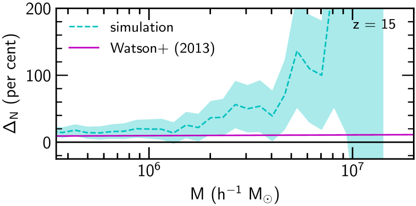
Figure 11: Comparison of the fractional difference $\Delta_{N}$ in halo mass function $N(>M)$ between our simulations and the simulations from Naoz et al. (2012) (cyan short-dashed) and between the Watson et al. (2013) curve, which is fit to $N$-body simulations, for the cosmology used in our work and the one used in Naoz et al. (2012) (magenta solid). The fractional difference is calculated as $\Delta_{N}=(N_{1}-N_{0})/N_{0}$, where $N_{0}$ are the data corresponding to our work and $N_{1}$ to Naoz et al. (2012), so $\Delta_{N}>0$ means there are more haloes in Naoz et al. (2012). Neither run includes $v_{\rm bc}$. The shaded cyan region indicates the combined 1$\sigma$ Poisson uncertainty on $N(>M)$ from the simulations.For $M\lesssim 4\times 10^{6}~{}h^{-1}~{}\mathrm{M}_{\odot}$ the difference in $N(>M)$ between the simulations is mostly consistent with the expected difference due to cosmology and halo mass definitions (i.e. the difference between the Watson et al. 2013 curves). Potential sources of the high-mass ($M\gtrsim 4\times 10^{6}~{}h^{-1}~{}\mathrm{M}_{\odot}$) discrepancy are discussed in the text.

However, the overall shape of our $\Delta_{N}$ is slightly different to Naoz et al. (2012); we match well below $\sim 3\times 10^{5}~{}h^{-1}~{}\mathrm{M}_{\odot}$ but show more relative suppression above this mass. This discrepancy is due, at least in part, to the different simulation codes used and the different white noise fields in the initial conditions. One further significant source of difference is the cosmologies used. Fig. 11 shows the difference expected at $z=15$ by comparing the analytic Watson et al. (2013) $N(>M)$ mass functions (magenta solid). From this, we would expect the Naoz et al. (2012) simulation to have $\sim 9~{}{\rm per~{}cent}$ more haloes with $M>3\times 10^{5}~{}h^{-1}~{}\mathrm{M}_{\odot}$. This increase in the number of haloes increases with mass and for $M>1\times 10^{7}~{}h^{-1}~{}\mathrm{M}_{\odot}$, we would expect $\sim 11~{}{\rm per~{}cent}$ more haloes in the Naoz et al. (2012) simulation. Indeed this is borne out by the simulations (cyan dashed), which show that the Naoz et al. (2012) simulations do produce more haloes at all masses. At higher masses, $\Delta_{N}$ diverges as the absolute number of haloes becomes small. As discussed earlier, Naoz et al. (2012) use the friends-of-friends groups as a starting point, which could be a source of the high-mass discrepancy in Fig. 11.

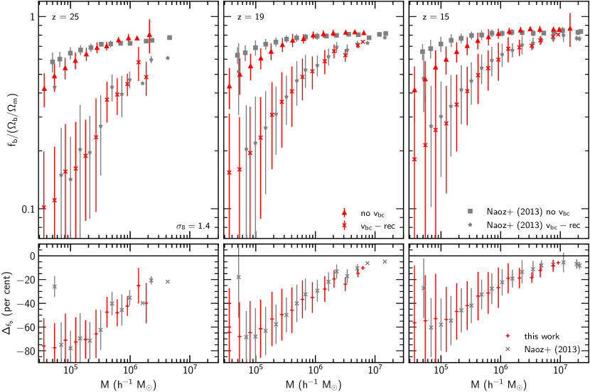
Figure 12: Binned baryon fraction $f_{\rm b}$ (top panels) and relative fractional difference $\Delta_{f_{\rm b}}$ between each run with $v_{\rm bc}$ to the run without, calculated with equation (12) (bottom panels). We show data from our simulations (red triangles, points and plusses) and from the Naoz et al. (2013) work (grey squares, stars and crosses). The panels show $z=25$ (left), $19$ (centre) and $15$ (right). The errorbars indicate the $1\sigma$ standard deviation in each mass bin (top panels) and the combined $1\sigma$ uncertainty (bottom panels). We find excellent agreement in the relative difference between our work and Naoz et al. (2013), and broad agreement in the absolute value of $f_{\rm b}$. Some slight disagreement in the absolute value could be due to the different choice of simulation methodology, since we employ an Eulerian code where Naoz et al. (2013) use a Lagrangian code.

Next, we turn our attention to the gas fraction of haloes, as studied in Naoz et al. (2013). Since we do not include star formation in these runs, the baryon fraction is simply the halo gas mass divided by the total halo mass

$$f_{\rm b}=\frac{M_{\rm g}}{M_{\rm g}+M_{\rm d}}.$$ (13)

Fig. 12 shows the binned gas fractions (top panel) for our and for the Naoz et al. (2013) simulations, each normalised to the cosmic mean $\Omega_{\rm b}/\Omega_{\rm m}$ for the appropriate cosmology, and the decrement (bottom panel) as defined in equation (12). We take the midpoint of the mass bin to be the mean of all the mass values in that bin. The binned gas fractions for Naoz et al. (2013) are slightly higher than in this work, though they exhibit roughly the same mass dependence. The agreement between the two simulations for the decrement is striking – they have an extremely similar mass dependence. There is some difference in the binned baryon fractions, in particular we find slightly more suppression at lower masses. This is likely due to differences in code used since, as mentioned previously, Naoz et al. (2013) used gadget2 (Springel, 2005), where we use ramses. There are well documented differences between Lagrangian (e.g. SPH) and Eulerian (e.g. AMR) codes (e.g. Agertz et al., 2007), and indeed it has been shown that numerical diffusion due to baryon-grid relative velocities can artificially smooth densities in Eulerian codes (Pontzen et al., 2020). In any case, we are not interested in comparing the merits of different codes, so by calculating the difference between the runs with and without $v_{\rm bc}$, we can remove artefacts due to the choice of code.

References

- Agertz et al. (2007) Agertz O., et al., 2007, Monthly Notices of the Royal Astronomical Society, 380, 963
- Ahn (2016) Ahn K., 2016, The Astrophysical Journal, 830, 68
- Ahn & Smith (2018) Ahn K., Smith B. D., 2018, The Astrophysical Journal, 869, 76
- Alam et al. (2017) Alam S., et al., 2017, Monthly Notices of the Royal Astronomical Society, 470, 2617
- Ali-Haïmoud et al. (2014) Ali-Haïmoud Y., Meerburg P. D., Yuan S., 2014, Physical Review D, 89, 083506
- Barkana (2016) Barkana R., 2016, Physics Reports, 645, 1
- Behroozi et al. (2013) Behroozi P. S., Wechsler R. H., Wu H.-Y., Busha M. T., Klypin A. A., Primack J. R., 2013, The Astrophysical Journal, 763, 18
- Bertschinger (2001) Bertschinger E., 2001, The Astrophysical Journal Supplement Series, 137, 1
- Beutler et al. (2017) Beutler F., Seljak U., Vlah Z., 2017, Monthly Notices of the Royal Astronomical Society, 470, 2723
- Bovy & Dvorkin (2013) Bovy J., Dvorkin C., 2013, The Astrophysical Journal, 768, 70
- Cain et al. (2020) Cain C., D’Aloisio A., Iršič V., McQuinn M., Trac H., 2020, arXiv e-prints, 2004, arXiv:2004.10209
- Chiou et al. (2018) Chiou Y. S., Naoz S., Marinacci F., Vogelsberger M., 2018, Monthly Notices of the Royal Astronomical Society, 481, 3108
- Chiou et al. (2019) Chiou Y. S., Naoz S., Burkhart B., Marinacci F., Vogelsberger M., 2019, The Astrophysical Journal, 878, L23
- Chiou et al. (2021) Chiou Y. S., Naoz S., Burkhart B., Marinacci F., Vogelsberger M., 2021, The Astrophysical Journal, 906, 25
- Chluba & Thomas (2011) Chluba J., Thomas R. M., 2011, Monthly Notices of the Royal Astronomical Society, 412, 748
- Chluba et al. (2010) Chluba J., Vasil G. M., Dursi L. J., 2010, Monthly Notices of the Royal Astronomical Society, 407, 599
- Cohen et al. (2016) Cohen A., Fialkov A., Barkana R., 2016, Monthly Notices of the Royal Astronomical Society, 459, L90
- Dalal et al. (2010) Dalal N., Pen U.-L., Seljak U., 2010, Journal of Cosmology and Astroparticle Physics, 11, 007
- Davis et al. (1985) Davis M., Efstathiou G., Frenk C. S., White S. D. M., 1985, The Astrophysical Journal, 292, 371
- Druschke et al. (2020) Druschke M., Schauer A. T. P., Glover S. C. O., Klessen R. S., 2020, Monthly Notices of the Royal Astronomical Society, 498, 4839
- Dubois & Teyssier (2008) Dubois Y., Teyssier R., 2008, Astronomy and Astrophysics, 477, 79
- Fialkov (2014) Fialkov A., 2014, International Journal of Modern Physics D, 23, 1430017
- Fialkov et al. (2012) Fialkov A., Barkana R., Tseliakhovich D., Hirata C. M., 2012, Monthly Notices of the Royal Astronomical Society, 424, 1335
- Fialkov et al. (2013) Fialkov A., Barkana R., Visbal E., Tseliakhovich D., Hirata C. M., 2013, Monthly Notices of the Royal Astronomical Society, 432, 2909
- Fialkov et al. (2018) Fialkov A., Barkana R., Cohen A., 2018, Physical Review Letters, 121, 011101
- Gill et al. (2004) Gill S. P. D., Knebe A., Gibson B. K., 2004, Monthly Notices of the Royal Astronomical Society, 351, 399
- Greif et al. (2011) Greif T. H., White S. D. M., Klessen R. S., Springel V., 2011, The Astrophysical Journal, 736, 147
- Hahn & Abel (2011) Hahn O., Abel T., 2011, Monthly Notices of the Royal Astronomical Society, 415, 2101
- Harris et al. (2020) Harris C. R., et al., 2020, Nature, 585, 357
- Hirano et al. (2017) Hirano S., Hosokawa T., Yoshida N., Kuiper R., 2017, Science, 357, 1375
- Hunter (2007) Hunter J. D., 2007, Computing in Science and Engineering, 9, 90
- Knebe et al. (2013) Knebe A., et al., 2013, Monthly Notices of the Royal Astronomical Society, 428, 2039
- Knollmann & Knebe (2009) Knollmann S. R., Knebe A., 2009, The Astrophysical Journal Supplement Series, 182, 608
- Komatsu et al. (2009) Komatsu E., et al., 2009, The Astrophysical Journal Supplement Series, 180, 330
- Lake et al. (2021) Lake W., Naoz S., Chiou Y. S., Burkhart B., Marinacci F., Vogelsberger M., Kremer K., 2021, The Astrophysical Journal, 922, 86
- Lewis et al. (2000) Lewis A., Challinor A., Lasenby A., 2000, The Astrophysical Journal, 538, 473
- Long et al. (2022) Long H., Givans J. J., Hirata C. M., 2022, Monthly Notices of the Royal Astronomical Society, 513, 117
- Magg et al. (2022) Magg M., et al., 2022, Monthly Notices of the Royal Astronomical Society
- Maio et al. (2011) Maio U., Koopmans L. V. E., Ciardi B., 2011, Monthly Notices of the Royal Astronomical Society, 412, L40
- McQuinn & O’Leary (2012) McQuinn M., O’Leary R. M., 2012, The Astrophysical Journal, 760, 3
- Muñoz (2019) Muñoz J. B., 2019, Physical Review D, 100, 063538
- Muñoz et al. (2022) Muñoz J. B., Qin Y., Mesinger A., Murray S. G., Greig B., Mason C., 2022, Monthly Notices of the Royal Astronomical Society, 511, 3657
- Murray et al. (2013) Murray S. G., Power C., Robotham A. S. G., 2013, Astronomy and Computing, 3, 23
- Naoz & Barkana (2005) Naoz S., Barkana R., 2005, Monthly Notices of the Royal Astronomical Society, 362, 1047
- Naoz & Barkana (2007) Naoz S., Barkana R., 2007, Monthly Notices of the Royal Astronomical Society, 377, 667
- Naoz & Narayan (2014) Naoz S., Narayan R., 2014, The Astrophysical Journal, 791, L8
- Naoz et al. (2012) Naoz S., Yoshida N., Gnedin N. Y., 2012, The Astrophysical Journal, 747, 128
- Naoz et al. (2013) Naoz S., Yoshida N., Gnedin N. Y., 2013, The Astrophysical Journal, 763, 27
- O’Leary & McQuinn (2012) O’Leary R. M., McQuinn M., 2012, The Astrophysical Journal, 760, 4
- Oñorbe et al. (2014) Oñorbe J., Garrison-Kimmel S., Maller A. H., Bullock J. S., Rocha M., Hahn O., 2014, Monthly Notices of the Royal Astronomical Society, 437, 1894
- Planck Collaboration et al. (2020) Planck Collaboration et al., 2020, Astronomy & Astrophysics, 641, A6
- Pontzen et al. (2020) Pontzen A., Rey M. P., Cadiou C., Agertz O., Teyssier R., Read J. I., Orkney M. D. A., 2020, arXiv e-prints, 2009, arXiv:2009.03313
- Popa et al. (2016) Popa C., Naoz S., Marinacci F., Vogelsberger M., 2016, Monthly Notices of the Royal Astronomical Society, 460, 1625
- Schaerer (2002) Schaerer D., 2002, Astronomy & Astrophysics, 382, 28
- Schauer et al. (2017) Schauer A. T. P., Regan J., Glover S. C. O., Klessen R. S., 2017, Monthly Notices of the Royal Astronomical Society, 471, 4878
- Schauer et al. (2019) Schauer A. T. P., Glover S. C. O., Klessen R. S., Ceverino D., 2019, Monthly Notices of the Royal Astronomical Society, 484, 3510
- Schauer et al. (2021) Schauer A. T. P., Glover S. C. O., Klessen R. S., Clark P., 2021, Monthly Notices of the Royal Astronomical Society, 507, 1775
- Seager et al. (1999) Seager S., Sasselov D. D., Scott D., 1999, The Astrophysical Journal Letters, 523, L1
- Slepian & Eisenstein (2015) Slepian Z., Eisenstein D. J., 2015, Monthly Notices of the Royal Astronomical Society, 448, 9
- Slepian et al. (2018) Slepian Z., et al., 2018, Monthly Notices of the Royal Astronomical Society, 474, 2109
- Smith & Lang (2019) Smith B., Lang M., 2019, The Journal of Open Source Software, 4, 1881
- Snaith et al. (2018) Snaith O. N., Park C., Kim J., Rosdahl J., 2018, Monthly Notices of the Royal Astronomical Society, 477, 983
- Springel (2005) Springel V., 2005, Monthly Notices of the Royal Astronomical Society, 364, 1105
- Stacy et al. (2011) Stacy A., Bromm V., Loeb A., 2011, The Astrophysical Journal, 730, L1
- Sunyaev & Zeldovich (1970) Sunyaev R. A., Zeldovich Y. B., 1970, Astrophysics and Space Science, Volume 7, Issue 1, pp.20-30, 7, 20
- Teyssier (2002) Teyssier R., 2002, Astronomy and Astrophysics, 385, 337