The genealogy of nearly critical branching processes in varying environment

Abstract

Building on the spinal decomposition technique in [16] we prove a Yaglom limit law for the rescaled size of a nearly critical branching process in varying environment conditional on survival. In addition, our spinal approach allows us to prove convergence of the genealogical structure of the population at a fixed time horizon – where the sequence of trees are envisioned as a sequence of metric spaces – in the Gromov–Hausdorff–Prohorov (GHP) topology. We characterize the limiting metric space as a time-changed version of the Brownian coalescent point process [46].

Beyond our specific model, we derive several general results allowing to go from spinal decompositions to convergence of random trees in the GHP topology. As a direct application, we show how this type of convergence naturally condenses the limit of several interesting genealogical quantities: the population size, the time to the most-recent common ancestor, the reduced tree and the tree generated by $k$ uniformly sampled individuals. As in a recent article by the authors [16], we hope that our specific example illustrates a general methodology that could be applied to more complex branching processes.

Keywords and Phrases. branching process in varying environment, Yaglom law, Kolmogorov asymptotics, spinal decomposition, many-to-few, Gromov–Hausdorff–Prohorov topology, coalescent point process

MSC 2010 subject classification. Primary 60J80; Secondary 60J90, 60F17

1 Introduction

Describing the genealogies of different population models as the size of the population gets large is a prominent task in the theory of mathematical population genetics, as well as in the study of branching processes and goes back at least to the two seminal papers of Kingman [35, 36]. As of today there is a vast literature on the genealogies of various type of populations models, see for example [5, 23, 33, 44, 46, 47], here we will focus among other topics on the scaling limit of the genealogy of nearly critical branching processes in varying environment conditional on survival, for a precise definition see Section 2.

The scope of this paper is two-fold, on the one hand we prove a Yaglom-type result [49] for the size of a nearly critical branching process in varying environment conditioned to survive for a long time, as well as a result on the scaling limit of the genealogy. For this purpose we prove a Kolmogorov-type asymptotics [37] for the probability of survival for an unusual long time, which might be interesting in its own right. On the other hand, our objective is to use this specific model to give an illustration of the techniques developed in [16, 20, 18, 22]. Our approach relies on new general results on random metric spaces that could be applied widely to branching processes with a critical behaviour. The spinal decomposition method in [16] gives an approach to study genealogies by showing convergence of random metric measure spaces in the Gromov-weak topology via a method of moments. To prove convergence of the $k$-th moment of a tree, a many-to-few formula allows to reduce this problem to calculating the distribution of a tree with $k$ leaves, the so-called $k$-spine tree. The distribution of the $k$-spine tree is obtained through a random change of measure, but allows the freedom to choose a suitable ansatz for the genealogy of the process. In order to make the $k$-spine method work, one would require the offspring distribution to have moments of all order, which is far from optimal conditions. However, due to a truncation argument, we are able to work under a second moment condition. Finally, we show how to reinforce the Gromov-weak convergence of the genealogy to a Gromov–Hausdorff–Prohorov convergence. By doing so, we obtain as a direct consequence of our main result the convergence of many interesting genealogical quantities.

In summary, a fraction of this paper will be dedicated to proving general results on random metric spaces. It is only at the end of the paper that this general formalism will be used to treat our specific problem as a (semi)-direct application. Along the way, we will obtain new criteria to obtain a Yaglom law for branching processes in varying environment (see Remark 2.2 below). We hope that this application will help convincing the reader that the abstract formalism introduced in [16, 20, 18, 22] (among others) and further developed in this paper is particularly well suited when treating general branching processes near criticality.

1.1 Relevant literature

The genealogical structure of branching processes is a topic that has drawn a lot of attention, especially in the critical case. Let us give a non-exhaustive account of some results related to our work. A first class of results focuses on the so-called reduced process [14, 50, 45], that counts the number of individuals having descendants at a fixed focal generation in the future. The limit of the reduced process is often expressed as a (time-inhomogeneous) pure birth process, see [33] for results in this direction for branching processes in varying environment. In the spirit of the theory of exchangeable coalescents, there has been an interest in describing the genealogy by sampling a fixed number $k$ of individuals uniformly at a given time [30, 26, 39]. We also want to point at [38] for an explicit construction of the genealogy of splitting trees as a discrete coalescent point process, which plays a central role in [39].

In this work, we show how the convergence of the previous two quantities, the reduced process and the genealogy of a uniform sample, as well as the convergence of the population size can be aggregated by viewing the population as a random ultrametric measure space converging in the Gromov–Hausdorff–Prohorov topology. Encoding trees as random metric spaces is a long-standing idea that has proved fruitful both for constant-size population models [12, 20] and for branching processes [2, 10]. Let us point at the following difference between our approach and more common convergence results in the Gromov–Hausdorff–Prohorov topology such as [2, 41, 43]. Here we consider the genealogy of the population at a fixed time horizon, whereas many works [2, 41, 43] are interested in the limit of the whole genealogical tree. Although in the limit one can construct the genealogy at a fixed time (the Brownian coalescent point process) from that of the whole tree (the Brownian continuum random tree), see [46], it is not straightforward to go from the convergence of the latter object to our type of convergence result. Also, from a technical point of view, the convergence of the whole tree is typically obtained by studying a height function, whereas our approach relies on a $k$-spine method.

The spinal decomposition of branching processes is widely used in the theory of branching processes, especially the case of the one-spine has been proven to be an important tool, see [42, 48, 17]. The classical Yaglom limit and the Kolmogorov estimate for critical Galton-Watson processes is obtained in [42] using this technique. We adapt the one spine decomposition from [42] to prove the Kolmogorov asymptotics for branching processes in varying environment, see Theorem 1. These techniques have been developed further for example in [27, 16] to allow for a $k$-spine construction, which in turn allows to compute higher moments of the tree by a random change of measure. Such a $k$-spine construction has also been used to extract information about the genealogy of several branching processes [26, 30, 16], and the current work follows a similar path. We also want to point at [19, 25] for a computation of higher order moments for general spatial branching processes, and the derivation of a Yaglom law in this context.

For an introduction to branching processes in varying environment (BPVE) we refer to the monograph of Kersting and Vatutin [34]. Lastly, the work of Kersting [32] gives a complete classification of critical branching processes in varying environment (among the other cases, supercritical, subcritical and asymptotically degenerate) as well as proving a Yaglom limit result. Later Cardona-Tobón and Palau in [8] managed to prove the Yaglom-type result for critical branching processes in varying environment by applying a two-spine decomposition and therefore providing a probabilistic proof of the result obtained by analytical methods in [32]. They make use of the remarkable fact that the distribution of the most recent common ancestor of two individuals can be found explicitly. Recently, in [33] Kersting managed to obtain the asymptotic distribution of the most recent common ancestor of all individuals living at some large time $n$. Our work is a continuation and extension of the aforementioned results, but does not build strongly on them, since we are dealing with nearly critical processes instead.

In the process of finishing this article we became aware of the work of Harris, Palau and Pardo [24] and of Conchon–Kerjan, Kious and Mailler [9]. In the former work, building on techniques of theirs developed in [27] and [8], the authors give a forward in time construction of the $k$-spine for a critical branching process in varying environment. Subsequently, via a change of measure relating the original branching process in varying environment and the $k$-spine tree they obtain their main result on the asymptotic distribution describing the splitting times for a uniform $k$-sample from the tree at large times, compare Theorem 2 (iii). Their results and the spinal decomposition are related to our work and are in the same spirit. However, due to the different points of view and approaches in their work and ours, we believe that these two papers can be seen as complementary to each other. We refer to Remark 2.2 and Remark 2.3 for a more in depth comparison. In the latter work [9], the authors derive the scaling limit of the whole tree structure of a branching process in i.i.d. random environment for the Gromov–Hausdorff–Prohorov topology. Their main result is consistent with ours in the sense that, under their hypothesis, the limit that we find (the Brownian coalescent point process) corresponds to the reduced tree at a given time of their limit (the Brownian continuum random tree). Nevertheless, as mentioned above, our type of result is not directly implied by the convergence of the whole tree and the techniques are different. Also, our hypothesis can be seen as more general, in the sense that we do not require the environment to have properties of i.i.d. sequences, and consider a sequence of nearly critical environments rather than a single strictly critical environment. In particular, stationary environments (and thus i.i.d. environments) can only lead to the Brownian coalescent point process in the limit, whereas we recover any time-change of a Brownian coalescent point process, including non-binary trees whenever the variance process has jumps.

1.2 Outline

The outline of this paper is as follows, first in Section 2 we will define precisely the notion of nearly critical branching process in varying environment and give some examples. We also state the Kolmogorov asymptotic (Theorem 1), as well as a first version of our main result (Theorem 2). In Section 3 we introduce the topologies on metric measure spaces necessary to state our main result in full generality and prove some continuity results for ultrametric spaces. The limiting object for the genealogy, the environmental coalescent point process, is introduced in Section 4 where we also derive some of its properties. Afterwards, the Kolmogorov asymptotics is proved in Section 5 and our main result (Theorem 3) is stated in full generality and proved in Section 6. Lastly, some results of technical nature are given in the Appendix A.

2 Model

Branching processes in varying environment (BPVE for short) are a natural generalisation of classical Galton–Watson processes, which allow for a changing offspring distribution between the generations. Throughout this work we will try to follow the notation of [34].

Let us start by properly defining the notion of a branching process in varying environment. Denote by $\mathcal{P}(\mathbb{N}_{0})$ the space of probability measures on $\mathbb{N}_{0}=\{0,1,2,\dots\}$ and let $v=(f_{1},f_{2},\dots)$ be a sequence of probability measures on $\mathbb{N}_{0}$.

Definition 2.1.

We call a process $(Z_{n},n\geq 0)$ a BPVE with environment $v=(f_{1},f_{2},\dots)$ with $v\in\mathcal{P}(N_{0})^{\mathbb{N}}$, if $(Z_{n},n\geq 0)$ has the representation

$$Z_{n}=\sum_{i=1}^{Z_{n-1}}\xi_{i,n},\quad Z_{0}=1,$$ (1)

where for each $n\geq 1$ the family $\{\xi_{i,n},i\geq 1\}$ consists of independent random variables with distribution $f_{n}$.

Note that we enforce the BPVE to consist of a single individual in generation $0$. In the subsequent parts it will be useful to identify measures $f\in\mathcal{P}(\mathbb{N}_{0})$ with their generating function

$$f(s)=\sum_{k=0}^{\infty}s^{k}f[k],\qquad s\in[0,1],$$ (2)

where $f[k]$, $k\geq 0$ denotes the weight of the distribution $f$ in $k$. Note that we will use the same symbol $f$ for the distribution as well as for the corresponding generating function $f(s)$. Recall that the first and second factorial moment of a random variable with distribution $f$ can be expressed as

$$f^{\prime}(1)=\sum_{k=1}^{\infty}kf[k],\qquad f^{\prime\prime}(1)=\sum_{k=2}^{\infty}k(k-1)f[k].$$ (3)

In the following we will consider a sequence $Z^{(N)}=\big{(}Z_{n}^{(N)},n\geq 0\big{)}$ of branching processes in varying environment indexed by $N$. That is we consider a sequence of environments $v^{(N)}=(f_{1}^{(N)},f_{2}^{(N)},\dots)$ and study the asymptotic probability for this process to survive $N$ generations as well as the asymptotic genealogy of a $k$ sample taken at a large time.

Due to the fact of working with a sequence of branching processes, all the quantities introduced so far as well as the quantities which will be introduced in the subsequent sections depend on $N$. Additionally, all expectations and probabilities will depend on $N$. For the convenience of the reader and for the reason to not overload the notation, we will drop the superscript $N$ most of the times, the reader should keep the implicit dependency of $N$ in mind. Furthermore, whenever there is a sum ranging from $1$ to $\lfloor Nt\rfloor$ we will abuse the notation and simply write $Nt$ as the upper limit.

Finally it is usual to encode the genealogy of branching processes as a random subset of the set of finite words

$$\mathcal{U}=\{\varnothing\}\cup\bigcup_{n\geq 1}\mathbb{N}^{n}.$$

A word $u=(u_{1},\dots,u_{n})$ is interpreted as an individual in the population living at generation $|u|\coloneqq n$. For two individuals $u,v\in\mathcal{U}$, we also use the notation $uv$ for their concatenation, and $u\wedge v$ for their most-recent common ancestor.

We can construct a random tree out of an independent collection $(K_{u},u\in\mathcal{U})$ of r.v. with $K_{u}\sim f_{|u|+1}$ by setting

$$T=\{u=(u_{1},\dots,u_{n}):\forall i\leq n,u_{i}\leq K_{(u_{1},\dots,u_{i-1})}\}.$$ (4)

This construction is carried out more carefully for BPVEs in [34, Section 1.4]. The variable $Z_{n}$ is recovered as the size of the $n$-th generation of $T$,

$$Z_{n}=\operatorname{Card}T_{n},\quad T_{n}\coloneqq\{u\in T:|u|=n\},\quad n\in\mathbb{N}.$$

2.1 Assumptions

In order to prove the main theorems, Theorem 1 and Theorem 3, we will work under the following assumptions on the sequence of environments $v=(f_{1},f_{2},\dots)$, which we call a nearly critical branching process in varying environment, recall that we do not denote the dependency of $v$ on $N$ explicitly. Let us introduce the following quantities,

$$\mu_{k}=\prod_{i=1}^{k}f_{i}^{\prime}(1),\quad\mu_{0}=1,$$ (5)

that is the expectation of the BPVE at time $k$, precisely $\mathbb{E}\left[Z_{k}\right]=\mu_{k}$. We call a sequence of branching processes in varying environment nearly critical, if for all

$$(\mu_{tN},t\geq 0)\to(e^{X_{t}},t\geq 0),\quad\text{ as }N\to\infty,$$ (6)

in the Skorohod topology for some càdlàg process $(X_{t},t\geq 0)$. (Having in mind the important case where the environment $v$ is a realization of an i.i.d. sequence, we use the terminology process for $(X_{t},t\geq 0)$ although it is a deterministic càdlàg function.) The next assumptions ensures that the variance between the generations does not fluctuate to strongly. Precisely, for some càdlàg non-decreasing function $\sigma^{2}(t):\mathbb{R}^{+}\to\mathbb{R}^{+}$ and some sequence $\kappa_{N}\to\infty$, we assume that for all $t\in\mathbb{R}^{+}$ such that $\sigma^{2}$ is continuous at $t$,

$$\frac{1}{\kappa_{N}}\sum_{k=1}^{Nt}f_{k}^{\prime\prime}(1)\to\sigma^{2}(t),\quad\text{ as }N\to\infty.$$ (7)

We also assume that $\sigma^{2}$ and $(X_{t},t\geq 0)$ do not jump at the same time. Lastly, we will enforce the following Lindeberg type condition

$$\forall\varepsilon>0,\quad\frac{1}{\kappa_{N}}\sum_{k=1}^{Nt}\mathbb{E}[\xi_{k}^{2}\mathbbm{1}_{\xi_{k}\geq\varepsilon\sqrt{\kappa_{N}}}]\to 0,\quad\text{as $N\to\infty$}$$ (8)

for a generic copy $\xi_{k}$ distributed as $f_{k}$. It will turn out that assumption (8) is only required to derive the asymptotics of the survival probability (the Kolmogorov asymptotics, see Theorem 1), and that all other results only rely on the following weaker assumption

$$\forall\varepsilon>0,\quad\frac{1}{\kappa_{N}}\sum_{k=1}^{Nt}\mathbb{E}[\xi_{k}^{2}\mathbbm{1}_{\xi_{k}\geq\varepsilon\kappa_{N}}]\to 0,\quad\text{as $N\to\infty$}.$$ (8’)

which prevents a single individual from having a large offspring of order $\kappa_{N}$. We believe that given (6) and (7) this assumption, which was already used in [7], is nearly optimal. For instance for Galton–Watson processes (8’) is known to be optimal for the process started from a population size of order $\kappa_{N}=N$ to converge to a Feller diffusion [21].

Remark 2.2.

Our definition of near criticality is directly inspired by that for Galton–Watson processes where we impose that the mean and the variance of the process converge. An alternative notion of criticality was proposed for BPVEs in [32] and was also further used in [33, 8, 24]. It relies on the behaviour of the following two series

$$\mu_{tN}\sum_{k=1}^{tN}\frac{1}{f_{k}^{\prime}(1)^{2}}\frac{f_{k}^{\prime\prime}(1)}{\mu_{k-1}}\sim\kappa_{N}\cdot\int_{[0,t]}e^{X_{t}-X_{s}}\sigma^{2}(ds)\to\infty\quad\text{as $N\to\infty$}$$

and

$$\sum_{k=1}^{tN}\frac{1}{f_{k}^{\prime}(1)^{2}}\frac{f_{k}^{\prime\prime}(1)}{\mu_{k-1}}\sim\kappa_{N}\cdot\int_{[0,t]}e^{-X_{s}}\sigma^{2}(ds)\to\infty\quad\text{as $N\to\infty$}$$

where the asymptotics under assumptions (6) and (7) are obtained in Lemma A.4. Since both series diverge, our BPVE would also be classified as critical in [32]. Assumptions (6) and (7) are not necessary for these series to diverge and can thus be thought of as restrictive in that sense.

It should be noted however that these stronger assumptions allow us to work with sequences of environments and lead to a notion of near criticality, whereas the aforementioned works consider fixed environment. Also we only need the mild moment condition (8) on the offspring size which we think is near optimal, whereas [8, 24] require a finite third moment, and [32, 33] a stronger second moment assumption. In particular, if (6) and (7) hold, the latter condition (assumption (B) in [32]) implies that for any sequence $K_{N}\to\infty$

$$\lim_{N\to\infty}\frac{1}{\kappa_{N}}\sum_{i=1}^{tN}\mathbb{E}[\xi_{k}^{2}\mathbbm{1}_{\xi_{k}>K_{N}}]=0$$ (9)

see Lemma A.6. Compare this to the weaker assumptions (8) and (8’). In particular, (9) prevents the limit process $\sigma^{2}$ from jumping, which in turn implies that the limit tree is binary.

2.2 Examples

Let us give some examples illustrating the conditions (6) and (7) and providing some examples which fit the class of models which we are considering here.

1. Consider a sequence of nearly critical Galton–Watson process $\big{(}Z^{(N)}_{n},n\geq 0\big{)}$ with offspring distribution $f^{(N)}$ such that $\xi^{(N)}\sim f^{(N)}$

   $$[f^{(N)}]^{\prime}(1)=1+\frac{\alpha}{N}+o\left(\frac{1}{N}\right)\quad\text{and}\quad[f^{(N)}]^{\prime\prime}(1)=\sigma^{2}+o(1),$$ (10)

   with $\alpha\in\mathbb{R}$ and $\sigma^{2}>0$. We then have

   $$\left(\mu_{sN},s\geq 0\right)=\left(\exp\left(\sum_{k=1}^{\lfloor sN\rfloor}\log(1+\alpha/N+o(1/N))\right),s\geq 0\right)\to\left(e^{\alpha s},s\geq 0\right),$$ (11)

   in the Skorohod topology, and the variance process (7) converges to $\sigma^{2}(t)=\sigma^{2}t$.

2. In [6] the authors considered a sequence of branching processes in random environment, such that the random first and second moment are given as independent copies of

   $$[F^{(N)}]^{\prime}(1)=1+\frac{\alpha}{N}+\frac{1}{\sqrt{N}}\zeta,\qquad[F^{(N)}]^{\prime\prime}(1)=\sigma^{2}+o(1),$$ (12)

   with $\alpha\in\mathbb{R}$, $\sigma^{2}>0$ and some zero mean random variable $\zeta$ with finite second moment. Then we have

   $$\left(\mu_{sN},s\geq 0\right)=\left(\exp\left(\sum_{k=1}^{\lfloor sN\rfloor}\log[F^{(N)}_{k}]^{\prime}(1)\right),s\geq 0\right)\to\left(\exp(\alpha^{\prime}s+B_{\rho s}),s\geq 0\right)\quad\text{in law}$$ (13)

   in the Skorohod topology, where $(B_{s},s\geq 0)$ is a standard Brownian motion and for some constants $\alpha^{\prime},\rho$ depending on the moments of $\zeta$.

3. The setting of the second example is easily adapted to cases where the corresponding random walk converges to a general Lévy process instead.

4. Let $p\in(0,1)$. Consider a varying environment where

   $$\forall k\in\tfrac{N}{2}+[0,N^{1-p}],\quad\mathbb{P}(\xi_{k}=i)=\begin{cases}\tfrac{1}{N^{p}},&\text{if $i=N^{p}$}\\ 1-\tfrac{1}{N^{p}},&\text{if $i=0$.}\end{cases}$$

   and the environment is constant elsewhere, with mean $1$ and variance $\beta$. Then the variance processes converges to the linear function $\beta t$ with a jump of size $1$ at $1/2$. Note that (8’) is fulfilled, whereas (8) is only fulfilled for $p<1/2$. By the same token, one can extend the construction to generate limiting varying environments where $\sigma^{2}$ is a subordinator and $X$ an arbitrary independent Lévy process.

2.3 Main results

We now discuss our two main results, namely the estimate for the survival probability and the scaling limit of the genealogy of nearly critical BPVEs.

Theorem 1 (Kolmogorov estimate).

Let $(Z_{n},n\geq 0)$ be a sequence of BPVE. For $t>0$ such that $t$ is a continuity point of $\sigma^{2}(t)$ and $\sigma^{2}(t)$ strictly increasing at $t$, then as $N\to\infty$ under the near critical assumptions (6), (7) and (8) we have

$$\mathbb{P}(Z_{tN}>0)\sim\frac{2}{\kappa_{N}}\frac{1}{\int_{0}^{t}e^{-X_{s}}\sigma^{2}(ds)}.$$ (14)

We note that in the case of critical or nearly critical Galton–Watson processes, Theorem 1 reduces to well known results, see [37] and [45]. The proof of Theorem 1 will be given in Section 5.

Our second main result, Theorem 3, shows that the genealogical structure of the BPVE, when envisioned as a random metric measure space, converges in the Gromov–Hausdorff–Prohorov topology to a limiting continuous tree, the environmental coalescent point process. Since this result might appear daunting at first sight and requires to introduce the formalism of random metric spaces, we postpone its formal statement until Section 6. Nevertheless, let us give a few direct consequences of our result for various genealogical quantities of the BPVE.

Stating our result requires some preliminary notation. For each $i\leq tN$, let $Z_{i,tN}$ be the number of individuals at generation $i$ having descendants at generation $tN$. The process $(Z_{i,tN},i\leq tN)$ is often referred to as the reduced process of the branching process [14]. Recall the definition of a Yule process, which is a Markov process with values in $\mathbb{N}$ that jumps from $k$ to $k+1$ at rate $k$. Also, on the event that $Z_{tN}>0$, let $(U_{1},\dots,U_{k})$ be $k$ individuals chosen uniformly at random from $T_{tN}$, the set of individuals at generation $tN$. Denote by $d_{T}(U_{i},U_{j})$ the time to the most recent common ancestor of $U_{i}$ and $U_{j}$. We introduce two distributions, which will describe the limiting distribution of the genealogical distances. Let

$$\forall s\leq t,\qquad\mathbb{P}\left(H\leq s\right)=\frac{1}{2\bar{\rho}_{t}}\int_{[t-s,t]}e^{X_{t}-X_{u}}\sigma^{2}(du),$$ (15)

with

$$\bar{\rho}_{t}\coloneqq\frac{1}{2}\int_{[0,t]}e^{X_{t}-X_{u}}\sigma^{2}(du),$$ (16)

in the literature concerning branching processes in varying environment, it is common to define $\rho_{n}=\sum_{k=1}^{n}\frac{f_{k}^{\prime\prime}(1)}{f_{k}^{\prime}(1)^{2}\mu_{k-1}}$ (for example [33],[8]), which up to a constant agrees with our choice, see Lemma A.4. To avoid confusion we chose a slightly different notation and explain this in more detail in Remark 2.3.

For $k\in\mathbb{N}$ and a sequence $(H_{1},\dots,H_{k-1})$ of independent random variables with distribution (15) we define the array $(H_{i,j};i,j\leq k)$ via

$$\forall i<j,\quad H_{i,j}=H_{j,i}=\max\{H_{i},\dots,H_{j-1}\},$$ (17)

with the convention that $\max\varnothing=0$. Additionally, for $\theta\geq 0$ we introduce $H^{\theta}$ with

$$\forall s\leq t,\qquad\mathbb{P}(H^{\theta}\leq s)=\frac{(1+\theta)\mathbb{P}(H\leq s)}{1+\theta\mathbb{P}(H\leq s)}.$$ (18)

Lastly, we introduce the array $(H^{\theta}_{i,j};i,j\leq k)$ in the same manner as in (17). Some motivation for these distribution in connection with coalescent point processes is provided in Section 4.2.

Theorem 2.

Fix $t>0$. Under the assumptions of Theorem 1 and conditional on $Z_{tN}>0$,

1. we have

   $$\mathscr{L}\left(\frac{Z_{Nt}}{Nt}\mid Z_{Nt}>0\right)\to\mathscr{E}\left(\bar{\rho}_{t}\right),\ \$$

   where $\mathscr{E}(x)$ denotes the exponential distribution with mean $x>0$;

2. for the reduced process we have

   $$(Z_{sN,tN},s<t)\to\left(Y\Big{(}\log\frac{\int_{[0,t]}e^{-X_{u}}\sigma^{2}(du)}{\int_{[s,t]}e^{-X_{u}}\sigma^{2}(du)}\Big{)},s<t\right)$$

   in the sense of finite-dimensional distribution at the continuity points of $\sigma^{2}$, and where $(Y(t),t\geq 0)$ is a Yule process. If $\sigma^{2}$ is continuous, the convergence holds in the Skorohod sense;

3. the law of the distance matrix $\big{(}\tfrac{d_{T}(U_{i},U_{j})}{N}\big{)}_{i,j}$ converges to the distribution of $(H_{\sigma_{i},\sigma_{j}})_{i,j}$ as in (15), where $\sigma$ is a uniform permutation of $\{1,\dots,k\}$ independent of $(H_{i,j})_{i,j}$. Let $\phi:\mathbb{R}^{k^{2}}\to\mathbb{R}$ be a bounded and continuous function, the distribution of the latter matrix is given by

   $$\mathbb{E}\big{[}\phi\big{(}(H_{i,j})_{i,j}\big{)}\big{]}=k\int_{0}^{\infty}\frac{1}{(1+\theta)^{2}}\Big{(}\frac{\theta}{1+\theta}\Big{)}^{k-1}\mathbb{E}\big{[}\phi\big{(}(H^{\theta}_{i,j})_{i,j}\big{)}\big{]}d\theta,$$

   where $\big{(}(H^{\theta}_{i,j})_{i,j}\big{)}$ has distribution (18).

In all three items of the previous result, the limiting random variable of interest can be written as the image of a limiting continuum random metric space – the environmental coalescent point process – introduced in Section 4. The previous convergence result is established by proving that the BPVE converges in the Gromov–Hausdorff–Prohorov topology, see Theorem 3, and computing the expectation of the corresponding functional for the limiting tree.

Finally, let us illustrate our result by specifying the previous corollary to our first example, a nearly critical Galton–Watson processes with mean $1+\alpha/N+o(1/N)$ and variance $\sigma^{2}+o(1)$. Theorem 1 becomes

$$\mathbb{P}\left(Z_{tN}>0\right)\sim\begin{dcases}\frac{1}{N}\frac{2}{\sigma^{2}t},\quad&\alpha=0\\ \frac{1}{N}\frac{2\alpha}{\sigma^{2}(1-e^{-\alpha t})},\quad&\alpha\neq 0.\end{dcases}$$

Note that the case $\alpha=0$ corresponds to the classical Kolmogorov asymptotics [37], whereas the case $\alpha\neq 0$ can be found in [45]. Furthermore, the first point of Theorem 2 yields

$$\mathscr{L}\left(\frac{Z_{Nt}}{Nt}\mid Z_{Nt}>0\right)\to\begin{dcases}\mathscr{E}\big{(}\tfrac{\sigma^{2}}{2}\big{)},\quad&\alpha=0\\ \mathscr{E}\big{(}\tfrac{\sigma^{2}}{2}\tfrac{e^{\alpha t}-1}{\alpha}\big{)},\quad&\alpha\neq 0.\end{dcases}$$

These are well-known asymptotics for nearly critical branching processes, see for instance [45]. In turn, point (iii) of Theorem 2 and a small calculation proves that the joint limiting distribution of the split times $s_{1},\dots,s_{k-1}\in[0,t]^{k-1}$ of the subtree spanned by $(U_{1},\dots,U_{k})$ has density $f(s_{1},s_{2},\dots,s_{k-1})$, such that

$$f(s_{1},s_{2},\dots,s_{k-1})=\begin{dcases}k\left(\frac{1}{t}\right)^{k-1}\int_{0}^{\infty}\frac{\theta^{k-1}}{(1+\theta)^{2}}\prod_{i=1}^{k-1}\frac{1}{1+\theta\frac{s_{i}}{t}}d\theta,\quad&\alpha=0\\ k(\alpha(e^{\alpha t}-1))^{k-1}\int_{0}^{\infty}\frac{\theta^{k-1}}{(1+\theta)^{2}}\prod_{i=1}^{k-1}\frac{e^{\alpha s_{i}}}{(\theta(e^{\alpha s_{i}}-1)+e^{\alpha t}-1)^{2}}d\theta,\quad&\alpha\neq 0\end{dcases}$$ (19)

which is exactly the limit in [26, Theorem 3] for $\alpha=0$. Finally, point (ii) shows that the reduced process is asymptotically distributed as the following time-changed Yule process,

$$\left(Y\Big{(}\log\frac{1-e^{-\alpha t}}{e^{-\alpha s}-e^{-\alpha t}}\Big{)},s<t\right)$$ (20)

which again is a known result, see [45, Remark 1]. Our work extends these results to the setting of nearly critical branching processes in varying environment.

Remark 2.3.

Let

$$\forall s\leq t,\quad G^{(N)}(s)=\frac{\rho_{s}^{(N)}}{\rho_{t}^{(N)}},\quad\rho_{s}^{(N)}=\sum_{k=1}^{sN}\frac{1}{f_{k}^{\prime}(1)^{2}}\frac{f_{k}^{\prime\prime}(1)}{\mu_{k-1}}.$$

The main result in [33] and [24] are respectively that, after making a time-rescaling $u=G^{(N)}(s)$, the reduced process and the law of a $k$ sample from a BPVE converge to the corresponding expressions for the Brownian CPP. Since $G^{(N)}(s)\to G(s)\coloneqq\frac{\bar{\rho}_{s}}{\bar{\rho}_{t}}$, (see Lemma A.4), reverting the limiting time-change, that is taking $s=F^{-1}(u)$, yields the environmental CPP (see Proposition 4.1). Thus points (ii) and (iii) of Theorem 2 are consistent with the results obtained in [33] and [24]. Note again that we work under different settings, see Remark 2.2.

3 Random metric measure spaces and Gromov topologies

Our main result shows the convergence of the genealogy of the BPVE, viewed as a random metric measure space. This section introduces the topological notions that are required to state this result, as well as some results regarding ultrametric spaces. We will need to work with two distinct topologies on the space of metric measure spaces: the Gromov-weak topology and the stronger Gromov–Hausdorff–Prohorov (GHP) topology.

The bulk of our work is dedicated to proving convergence in the Gromov-weak topology which is introduced in Section 3.1.1. In this topology, convergence in distribution is strongly connected to convergence of moments of the metric space, which are computed out of samples from the metric space. We show in Section 3.1.2 how these moments can be efficiently computed for branching processes using $k$-spine techniques and a many-to-few formula. Applying this method of moments requires the reproduction laws to have moments of any order, whereas our convergence result only requires a finite moment of order two. To overcome this difficulty, we use a truncation procedure similar to that used in [26]. Section 3.1.3 contains some perturbation results that are used to prove that the truncated version of the BPVE remains close in the Gromov-weak topology to the original BPVE.

Although proving convergence in distribution in the Gromov-weak topology is made considerably easier by the method of moments, this topology is too weak to ensure the convergence of some natural statistics of genealogies, such as the convergence of the reduced process. This motivates the introduction of a stronger topology in Section 3.2, the Gromov–Hausdorff–Prohorov (GHP) topology. Once convergence is established for the Gromov-weak topology by computing moments, we will show how to strengthen it to a GHP convergence through a simple tightness argument that should apply broadly to critical branching processes satisfying a Yaglom law.

3.1 Convergence in the Gromov-weak topology

3.1.1 The Gromov-weak topology

We briefly recall the definition of the Gromov-weak topology and some of its properties that are needed in this work. The reader is referred to [20, 18, 22] for a more complete account.

A metric measure space is a triple $[X,d,\nu]$ such that $(X,d)$ is a complete separable metric space and $\nu$ is a finite measure on the corresponding Borel $\sigma$-field. Given some $k\geq 1$ and a bounded continuous map $\phi\colon[0,\infty)^{k\times k}\to\mathbb{R}$, we define a functional $\Phi$ on the space of metric measure spaces, called a polynomial, as

$$\Phi\big{(}X,d,\nu\big{)}=\int_{X^{k}}\phi\big{(}(d(x_{i},x_{j}))_{i,j\leq k}\big{)}\nu(dx_{1})\dots\nu(dx_{k}).$$

The Gromov-weak topology is defined as the topology induced by the polynomials, that is the smallest topology making all polynomials continuous. The Gromov-weak topology allows us to define a random metric measure space, as a random variable with values in metric measure spaces, endowed with the Gromov-weak topology and the corresponding Borel $\sigma$-field. The moment of a random metric measure space associated to $\Phi$ is the expectation of the corresponding polynomial.

Recall the tree construction of the BPVE from Section 2, and the notation $T_{n}$ for the $n$-th generation of the process. Let the tree distance be

$$\forall u,v\in T_{n},\quad d_{T}(u,v)=n-|u\wedge v|$$

and consider the measure

$$\lambda_{n}=\sum_{u\in T_{n}}\delta_{u}.$$

Then $[T_{n},d_{T},\lambda_{n}]$ is the random metric measure space encoding the genealogy of generation $n$ of the BVPE.

The appeal of the Gromov-weak topology is well illustrated by the following result, which connects convergence in distribution for the Gromov-weak topology to the convergence of moments, see [10, Lemma 2.8].

Proposition 3.1 (Method of moments).

Consider a sequence $([X_{n},d_{n},\nu_{n}],n\geq 1)$ of random metric measure spaces such that

$$\forall\Phi,\quad\mathbb{E}\big{[}\Phi\big{(}X_{n},d_{n},\nu_{n}\big{)}\big{]}\to\mathbb{E}\big{[}\Phi\big{(}X,d,\nu\big{)}\big{]}<\infty,$$

for some limiting space $[X,d,\nu]$. Then, if the limiting space further fulfils that

$$\limsup_{k\to\infty}\frac{\mathbb{E}[\nu(X)^{k}]^{1/k}}{k}<\infty,$$

the sequence $([X_{n},d_{n},\nu_{n}],n\geq 1)$ converges to $[X,d,\nu]$ in distribution for the Gromov-weak topology.

Remark 3.2 (Identification of the limit).

The previous result requires to first identify the limit of the sequence $[X_{n},d_{n},\nu_{n}]$, and then to prove convergence to the moments of this limit. Compare to the usual method of moments for real random variables where convergence of the moments provides existence of the limit. For ultrametric spaces, which are the metric notion of a genealogy at a given time horizon, it is possible to improve Proposition 3.1 in this direction, see [16, Section 4]. This relies on enlarging the Gromov-weak topology to non-separable ultrametric spaces, using a de Finetti representation for exchangeable coalescents obtained in [15].

3.1.2 The many-to-few formula

Applying the previous result to prove convergence in the Gromov-weak topology requires to compute the moments of the BPVE. In the context of discrete trees, we find it easier to work with factorial moments. The factorial moment of order $k$ associated to $\phi$ of a BPVE is simply

$$\mathbb{E}\big{[}\Phi[T_{N},d_{T},\lambda_{N}]\big{]}=\mathbb{E}\Big{[}\sum_{\begin{subarray}{c}u_{1},\dots,u_{k}\in T_{N}\\ \text{$(u_{i})$ distinct}\end{subarray}}\phi\big{(}(d_{T}(u_{i},u_{j}))_{i,j}\big{)}\Big{]}.$$

We want to express this moment in terms of a simpler tree with $k$ leaves, called the $k$-spine tree. There exist different choices for the distribution of this tree. We choose to follow the approach in [16], where the $k$-spine tree is constructed as a discrete coalescent point process. More precisely, for each $N$ consider a probability distribution $(p_{i},i\leq N)$ on $\{1,\dots,N\}$. (As in the rest of the paper we make the dependency on $N$ implicit). Let $(H^{(N)}_{i};\,i\geq 1)$ be a sequence of i.i.d. random variables with distribution $(p_{i},i\leq N)$ and as in (17) introduce

$$\forall i<j,\quad H^{(N)}_{i,j}=H^{(N)}_{j,i}=\max\{H^{(N)}_{i},H^{(N)}_{i+1},\dots,H^{(N)}_{j-1}\}.$$

The array $(H^{(N)}_{i,j};\,i,j\leq k)$ corresponds to the pairwise distances between the leaves of a discrete tree that we denote by $S_{k}$. Following the notation in [16] we will denote the distribution of this array by $\mathbb{Q}^{k,N}$. See Figure 1 for an illustration of the construction of this tree, or Appendix A.1 for a rigorous definition. For each vertex $u\in S_{k}$, we further denote by $d_{u}$ the out-degree of $u$, and by $|u|$ the distance from $u$ to the root. A branch point is any vertex $u$ with $d_{u}>1$. The set of branch points of $S_{k}$ is denoted by $B$.

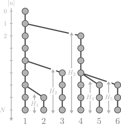
Figure 1: Illustration of the construction of the $k$-spine tree $S_{k}$, for $k=6$.

The many-to-few formula relates the factorial moments of a branching process to the distribution of $S_{k}$. It involves a random bias, that we denote by $\Delta_{k}$, which has the following expression in the context of branching processes with varying environment,

$$\Delta_{k}=k!\,\mu_{N}^{k}\cdot\prod_{u\in B}\frac{1}{(p_{N-|u|}\mu_{|u|})^{d_{u}-1}}\frac{1}{d_{u}!}\frac{f^{(d_{u})}_{|u|+1}(1)}{f^{\prime}_{|u|+1}(1)^{d_{u}}},$$ (21)

where $f^{(d_{u})}_{|u|+1}$ denotes the $d_{u}$-th derivative of the generating function of the offspring distribution in generation $|u|$. Note that we have included the $k!$ term in the definition of $\Delta_{k}$ compared to [16].

Proposition 3.3 (Many-to-few).

For any $k\geq 1$ and any measurable map $\phi\colon[0,\infty)^{k\times k}\to[0,\infty)$ we have

$$\mathbb{E}\Big{[}\sum_{\begin{subarray}{c}u_{1},\dots,u_{k}\in T_{N}\\ \text{$(u_{i})$ distinct}\end{subarray}}\phi\big{(}(d_{T}(u_{i},u_{j}))_{i,j}\big{)}\Big{]}=\mathbb{Q}^{k,N}\Big{[}\Delta_{k}\cdot\phi\big{(}(H^{(N)}_{\sigma_{i},\sigma_{j}})_{i,j}\big{)}\Big{]}$$

where, under $\mathbb{Q}^{k,N}$, $\sigma$ is an independent permutation $[k]$.

Proof.

The result will follow from the many-to-few formula derived in [16, Proposition 2] for branching processes with a general type space. We interpret time in a branching process with varying environment as a type, an individual $u$ at generation $n$ is endowed with type $X_{u}=n$. Using the formula in [16] only requires to find an appropriate harmonic function for the process. Since the process $(Z_{n}/\mu_{n},n\geq 0)$ is a non-negative martingale, this readily implies that

$$h\colon n\mapsto 1/\mu_{n}$$

is a harmonic function. The result now follows from [16, Proposition 2] by recalling that $f^{(k)}_{n+1}(1)$ is the $k$-th factorial moment of the offspring distribution of an individual living at generation $n$. It might help the reader to note that, in the current work, the height of the $i$-th branch point is encoded as its distance to the leaves $H_{i}$, whereas in [16] it is encoded as the distance to the root $W_{i}$, so that $H_{i}=N-W_{i}$. ∎

3.1.3 Truncation in the Gromov-weak topology

Applying the method of moments requires to carry out a truncation of the reproduction laws for all moments to be finite. In order to deduce from the convergence of the truncated BPVE that of the original BPVE, we need to show that the two trees remain close with large probability for an adequate choice of distance between trees. It turns out that one can define a distance on the space of metric measure spaces that induces the Gromov-weak topology [20, 18, 22]. There are several formulations for such a distance, we work with the so-called polar Gromov–Prohorov distance from [18]. The distance between two metric measure spaces is defined as

$$d_{\mathrm{pGP}}\big{(}[X,d,\nu],[X^{\prime},d^{\prime},\nu^{\prime}]\big{)}=|\nu(X)-\nu^{\prime}(X^{\prime})|+d_{\mathrm{GP}}\big{(}[X,d,\hat{\nu}],[X^{\prime},d^{\prime},\hat{\nu}^{\prime}]\big{)}$$

where $d_{\mathrm{GP}}$ stands for the Gromov–Prohorov distance, and $\hat{\nu}=\nu/\nu(X)$, with the same definition for $\hat{\nu}^{\prime}$. In turn, the Gromov–Prohorov distance is defined as

$$d_{\mathrm{GP}}\big{(}[X,d,\hat{\nu}],[X^{\prime},d^{\prime},\hat{\nu}^{\prime}]\big{)}=\inf_{Z,\phi,\phi^{\prime}}d_{\mathrm{P}}(\hat{\nu}\circ\phi^{-1},\hat{\nu}^{\prime}\circ(\phi^{\prime})^{-1})$$

where the infimum is taken over all metric spaces $(Z,d_{Z})$ and isometric embeddings $\phi\colon X\hookrightarrow Z$ and $\phi^{\prime}\colon X^{\prime}\hookrightarrow Z$, $\hat{\nu}\circ\phi^{-1}$ is the pushforward measure of $\hat{\nu}$ through the map $\phi$, and $d_{\mathrm{P}}$ is the Prohorov distance on $(Z,d_{Z})$. The following simple lemma will be key to controlling the distance between the truncated and the original tree.

Lemma 3.4.

Consider a metric measure space $(X,d,\nu)$. Let $X^{\prime}$ be a closed subset of $X$, and $\nu^{\prime}$ be the restriction of $\nu$ to $X^{\prime}$. Then

$$d_{\mathrm{pGP}}\big{(}[X,d,\nu],[X^{\prime},d,\nu^{\prime}]\big{)}\leq\nu(X\setminus X^{\prime})+\Big{(}1-\frac{\nu(X^{\prime})}{\nu(X)}\Big{)}.$$

Proof.

It is only necessary to bound the Gromov–Prohorov distance between the two re-normalized spaces to prove the Lemma. Since both of them are already isometrically embedded in $X$, we have

$$d_{\mathrm{GP}}\big{(}[X,d,\tfrac{\nu}{\nu(X)}],[X^{\prime},d^{\prime},\tfrac{\nu^{\prime}}{\nu(X^{\prime})}]\big{)}\leq d_{\mathrm{P}}\big{(}\tfrac{\nu}{\nu(X)},\tfrac{\nu^{\prime}}{\nu(X^{\prime})}\big{)}\leq d_{\mathrm{TV}}\big{(}\tfrac{\nu}{\nu(X)},\tfrac{\nu^{\prime}}{\nu(X^{\prime})}\big{)},$$

where $d_{\mathrm{TV}}$ denotes the total variation metric. Since $\frac{\nu^{\prime}(\cdot)}{\nu(X^{\prime})}=\frac{\nu(\cdot)}{\nu(X)}\frac{\nu(X)}{\nu(X^{\prime})}$ on $X^{\prime}$ we immediately obtain

$$d_{\mathrm{TV}}\left(\frac{\nu}{\nu(X)},\frac{\nu^{\prime}}{\nu(X)}\right)=\sup_{A\in\mathcal{B}(X)}\left|\frac{\nu(A)}{\nu(X)}-\frac{\nu(A\cap X^{\prime})}{\nu(X^{\prime})}\right|=1-\frac{\nu(X^{\prime})}{\nu(X)},$$ (22)

which finishes the proof. ∎

The practical interest of the previous result lies in the following corollary.

Corollary 3.5.

Let $([X_{n},d_{n},\nu_{n}],n\geq 1)$ be a sequence of random metric measure spaces and, for $n\geq 1$, let $X^{\prime}_{n}\subseteq X_{n}$ be a closed subset. Suppose that as $n\to\infty$

1. we have $|\nu_{n}(X_{n})-\nu_{n}(X^{\prime}_{n})|\to 0$ in probability;

2. we have $[X^{\prime}_{n},d_{n},\nu_{n}]\to[X,d,\nu]$ in distribution for the Gromov-weak topology and $\nu(X)>0$ a.s.;

then $[X_{n},d_{n},\nu_{n}]$ converges to $[X,d,\nu]$ in distribution for the Gromov-weak topology.

Proof.

The result will follow by showing that the Gromov–Prohorov distance between the two spaces converges to $0$ in probability. By Lemma 3.4, we have that

$$\mathbb{P}\big{(}d_{\mathrm{pGP}}\big{(}[X_{n},d_{n},\nu_{n}],[X^{\prime}_{n},d_{n},\nu_{n}]\big{)}\geq 2\varepsilon\big{)}\\ \leq\mathbb{P}(\nu_{n}(X_{n})-\nu_{n}(X^{\prime}_{n})>\varepsilon)+\mathbb{P}(\nu_{n}(X_{n})-\nu_{n}(X^{\prime}_{n})>\varepsilon\nu_{n}(X_{n})).$$

The first term goes to $0$ by our assumptions. For the second term, note that for any $\varepsilon^{\prime}>0$,

$$\mathbb{P}(\nu_{n}(X_{n})-\nu_{n}(X^{\prime}_{n})>\varepsilon\nu_{n}(X_{n}))\leq\mathbb{P}(\nu_{n}(X_{n})-\nu_{n}(X^{\prime}_{n})>\varepsilon\varepsilon^{\prime})+\mathbb{P}(\nu_{n}(X^{\prime}_{n})<\varepsilon^{\prime}).$$

The first term goes to $0$ by our assumption while the second term can be made arbitrarily small by using the convergence of $\nu_{n}(X^{\prime}_{n})$ to $\nu(U)$ and that $\mathbb{P}(\nu(U)=0)=0$. Since the distance between the two spaces converges to $0$ in probability, they have to converge to the same limit in distribution. ∎

3.2 The Gromov–Hausdorff–Prohorov topology

We now turn to the definition of a second topology, the GHP topology. It is only defined for metric measure spaces that are compact. Consider two compact metric measure spaces $[X,d,\nu]$ and $[X^{\prime},d^{\prime},\nu^{\prime}]$. The GHP distance between these spaces is defined as

$$d_{\mathrm{GHP}}\big{(}[X,d,\nu],[X^{\prime},d^{\prime},\nu^{\prime}]\big{)}=\inf_{Z,\phi,\phi^{\prime}}\{d_{\mathrm{P}}(\nu\circ\phi^{-1},\nu^{\prime}\circ(\phi^{\prime})^{-1})+d_{\mathrm{H}}(\phi(X),\phi^{\prime}(X^{\prime}))\}$$

where the infimum is taken over all metric spaces $(Z,d_{Z})$ and isometric embeddings $\phi\colon X\hookrightarrow Z$ and $\phi^{\prime}\colon X^{\prime}\hookrightarrow Z$. In the previous expression, $\nu\circ\phi^{-1}$ refers to the push-forward of $\nu$ by $\phi$, $d_{\mathrm{H}}$ to the Hausdorff distance on $Z$, and $d_{\mathrm{P}}$ to the Prohorov distance on $Z$. The GHP topology is the topology generated by the distance $d_{\mathrm{GHP}}$. We refer to [1] for properties of this topology.

Some caution should be used regarding the state spaces of the two topologies. Two metric measure spaces are indistinguishable in the Gromov-weak topology iff there exists a measure-preserving isometry between the supports of their respective measures, see around [20, Proposition 2.6]. In contrast, two metric measure spaces are indistinguishable in the Gromov–Hausdorff–Prohorov topology iff there exists a measure-preserving isometry between the whole spaces, see for instance [1, Section 2.2]. For the purpose of this discussion, let us say that the spaces are Gw-isometric in the former case, and GHP-isometric in the latter case. For the topologies to be separated, it is necessary to choose as state space equivalence classes of Gw-isometric or GHP-isometric spaces respectively. However, since two Gw-isometric spaces are not GHP-isometric in general, these state spaces do not coincide. Thus, we should always mention with respect to which topology is a random metric measure space defined.

In practice, since the GHP topology is stronger than the Gromov-weak topology, a random metric measure space for the GHP topology can always be seen as a random element of the Gromov-weak topology. Informally, this amounts to forgetting the metric structure of points that do not belong to the support of the measure. Conversely, consider the map

$$[X,d,\nu]\mapsto[\operatorname{supp}\nu,d,\nu].$$ (23)

This map extends uniquely to a map from Gw-isometry classes to GHP-isometry classes. Thus, by taking the image under the map (23), we can in turn see a random element of the Gromov-weak topology as a random element of the GHP topology.

When considering metric measure spaces with full support, as is the case in this work, this distinction vanishes. In particular for such spaces, the distribution under the GHP and Gromov-weak topology coincide. We record this as a lemma. (Note that, of course, even in this case the two topologies do not lead to the same notion of convergence in distribution.) For an in depth discussion of these questions, see [3].

Lemma 3.6.

Let $[X_{1},d_{1},\nu_{1}]$ and $[X_{2},d_{2},\nu_{2}]$ be two random compact metric measure spaces in the GHP topology such that $\operatorname{supp}\nu_{1}=X_{1}$ and $\operatorname{supp}\nu_{2}=X_{2}$ almost surely. The two spaces $[X_{1},d_{1},\nu_{1}]$ and $[X_{2},d_{2},\nu_{2}]$ have the same distribution in the GHP topology iff they have the same distribution in the Gromov-weak topology.

3.2.1 Ultrametric spaces and reduced processes

All metric spaces that are considered in this work are constructed as genealogies of population models at a fixed time horizon. They all have the further property of being ultrametric spaces. A metric space $(U,d)$ is called ultrametric if it fulfils the stronger triangle inequality

$$\forall x,y,z\in U,\quad d(x,y)\leq\max\{d(x,z),d(z,y)\}.$$

In this section we construct the reduced process associated to a general ultrametric space and prove that the application mapping an ultrametric space to its reduced process is continuous in the GHP topology.

A well-known property of ultrametric spaces is that the set of open balls of a given radius form a partition of the space, that is,

$$x\sim_{t}y\iff d(x,y)<t$$

is an equivalence relation. We will use the notation $B_{x,t}(U)=\{y\in U:d(x,y)<t\}$ for the open ball of radius $t$ around $x$, and

$$B_{t}(U)=\{B_{x,t}(U),x\in U\}$$

for the set of balls of radius $t$ of an ultrametric space $(U,d)$. In the genealogical interpretation of an ultrametric space, a ball of radius $t$ corresponds to the set of individuals sharing a common ancestor at time $t$ in the past. Thus, we can envision $B_{t}(U)$ as the set of ancestral lineages of the population at time $t$ in the past. This motivates the introduction of the process

$$\forall t>0,\quad L_{t}(U)=\operatorname{Card}B_{t}(U)$$

counting the number of ancestral lines, which we will refer to as the reduced process of the ultrametric space $(U,d)$. (Note the time reversal compared to the usual definition of a reduced process: time is flowing backward and not forward.)

The main result of this section shows that the convergence of the reduced process is a consequence of the convergence of the ultrametric spaces in the Gromov–Hausdorff–Prohorov topology. Actually, defining the reduced process does not require the ultrametric space to be equipped with a measure, and we only need the ultrametric spaces to converge in the weaker Gromov–Hausdorff topology. It is the topology associated to the Gromov–Hausdorff distance

$$d_{\mathrm{GH}}\big{(}[X,d],[X^{\prime},d^{\prime}]\big{)}=\inf_{Z,\phi,\phi^{\prime}}d_{\mathrm{H}}(\phi(X),\phi^{\prime}(X^{\prime})),$$

where the infimum is taken over all metric spaces $(Z,d_{Z})$ and isometric embeddings $\phi\colon X\hookrightarrow Z$ and $\phi^{\prime}\colon X^{\prime}\hookrightarrow Z$.

Proposition 3.7.

Suppose that $(U_{n},d_{n},n\geq 1)$ is a sequence of compact ultrametric spaces converging in the Gromov–Hausdorff topology to $(U,d)$. Then,

$$(L_{t}(U_{n}),t>0)\to(L_{t}(U),t>0)\quad\text{as $N\to\infty$}$$

in the sense of finite dimensional convergence at each continuity point of $(L_{t}(U),t>0)$. If $(U,d)$ is binary, that is, $(L_{t}(U),t>0)$ only makes jumps of size $1$, the convergence also holds in the Skorohod space $\mathbb{D}([t_{0},\infty))$ for all continuity point $t_{0}>0$ of the reduced process.

Our proof of this result is based on the following lemma.

Lemma 3.8.

Let $(U,d,\nu)$ and $(U^{\prime},d^{\prime},\nu^{\prime})$ be two compact ultrametric measure spaces such that

$$d_{\mathrm{GH}}\big{(}[U,d],[U^{\prime},d^{\prime}]\big{)}<\varepsilon$$

and let $t$ be such that $B_{t+3\varepsilon}(U^{\prime})=B_{t-3\varepsilon}(U^{\prime})$. Then we can find a bijection $\psi$ between $B_{t}(U)$ and $B_{t}(U^{\prime})$. If furthermore

$$d_{\mathrm{GHP}}\big{(}[U,d,\nu],[U^{\prime},d^{\prime},\nu^{\prime}]\big{)}<\varepsilon,$$

then

$$\forall B\in B_{t}(U),\quad|\nu(B)-\nu^{\prime}(\psi(B))|<\varepsilon.$$

Proof.

Fix a space $(Z,d_{Z})$ and isometries $\phi\colon U\hookrightarrow Z$ and $\phi^{\prime}\colon U^{\prime}\hookrightarrow Z$ with $d_{\mathrm{H}}(\phi(U),\phi^{\prime}(U^{\prime}))<\varepsilon$. Define a relation $R\subseteq U\times U^{\prime}$ through

$$(x,x^{\prime})\in R\iff d_{Z}(\phi(x),\phi^{\prime}(x^{\prime}))<\varepsilon.$$

It is well-known that, since $d_{\mathrm{GH}}([U,d],[U^{\prime},d^{\prime}])<\varepsilon$, $R$ is a correspondence, in the sense that for any $x\in U$, there is $x^{\prime}\in U^{\prime}$ with $(x,x^{\prime})\in R$ and conversely, see [13, Theorem 4.11]. Now, for any ball $B\in B_{t}(U)$ and $B^{\prime}\in B_{t}(U^{\prime})$ define a new relation $\tilde{R}$ through

$$(B,B^{\prime})\in\tilde{R}\iff\exists x\in B,x^{\prime}\in B^{\prime},\;(x,x^{\prime})\in R.$$

If we can prove that $\tilde{R}$ is one-to-one in the sense that for any $B\in B_{t}(U)$ there is a unique $B^{\prime}\in B_{t}(U^{\prime})$ with $(B,B^{\prime})\in\tilde{R}$, then $B_{t}(U)$ and $B_{t}(U^{\prime})$ are in bijection. First we show that for a given $B\in B_{t}(U)$, there is a most one $B^{\prime}\in B_{t}(U^{\prime})$ with $(B,B^{\prime})\in\tilde{R}$. Let $(x,x^{\prime})\in R$ and $(y,y^{\prime})\in R$ with $d(x,y)<t$. Then

$$d^{\prime}(x^{\prime},y^{\prime}) =d_{Z}(\phi^{\prime}(x^{\prime}),\phi^{\prime}(y^{\prime}))$$

$$\leq d_{Z}(\phi(x),\phi(y))+d_{Z}(\phi(x),\phi^{\prime}(x^{\prime}))+d_{Z}(\phi(y),\phi^{\prime}(y^{\prime}))$$

$$<t+2\varepsilon.$$

Since the $d^{\prime}$-balls of radius $t+2\varepsilon$ and $t$ are the same, $d^{\prime}(x^{\prime},y^{\prime})<t$, showing that the balls of radius $t$ to which $x^{\prime}$ and $y^{\prime}$ belong are the same. Now, since $R$ is a correspondence, for any $B$ with $x\in B$, there exists $x^{\prime}$ such that $(x,x^{\prime})\in R$. Thus $(B,B_{x^{\prime},t}(U^{\prime}))\in\tilde{R}$, proving that for each $B$ there is at least one $B^{\prime}$ with $(B,B^{\prime})\in\tilde{R}$. This constructs the required bijection $\psi$.

Let us now prove the second part of the result. Consider $(B,B^{\prime})\in\tilde{R}$ and $x\in B$, $x^{\prime}\in B^{\prime}$ with $(x,x^{\prime})\in R$. Then

$$\nu(B) =\nu\circ\phi^{-1}(\{z:d_{Z}(z,\phi(x))<t\})$$

$$\leq\nu\circ\phi^{-1}(\{z:d_{Z}(z,\phi^{\prime}(x^{\prime}))<t+\varepsilon)\})$$

$$\leq\nu^{\prime}\circ(\phi^{\prime})^{-1}(\{z:d_{Z}(z,\phi^{\prime}(x^{\prime}))<t+2\varepsilon)\})+\varepsilon$$

$$=\nu^{\prime}(\{y^{\prime}:d^{\prime}(x^{\prime},y^{\prime})<t+2\varepsilon\})+\varepsilon$$

$$=\nu^{\prime}(B^{\prime})+\varepsilon$$

where in the second line we have used that $d_{Z}(\phi(x),\phi^{\prime}(x^{\prime}))<\varepsilon$, in the third line the definition of the Prohorov distance, and in the last line that the balls of radius $t+2\varepsilon$ and $t$ of $U^{\prime}$ are the same. Conversely

$$\nu^{\prime}(B^{\prime}) =\nu^{\prime}(\{y^{\prime}:d^{\prime}(x^{\prime},y^{\prime})<t-2\varepsilon\})$$

$$=\nu^{\prime}\circ(\phi^{\prime})^{-1}(\{z:d_{Z}(z,\phi^{\prime}(x^{\prime}))<t-2\varepsilon\})$$

$$\leq\nu\circ\phi^{-1}(\{z:d_{Z}(z,\phi^{\prime}(x^{\prime}))<t-\varepsilon)\})+\varepsilon$$

$$\leq\nu\circ\phi^{-1}(\{z:d_{Z}(z,\phi(x))<t)\})+\varepsilon$$

$$=\nu(B)+\varepsilon.$$

This shows that $|\nu(B)-\nu^{\prime}(B^{\prime})|<\varepsilon$ and proves the second part of the result. ∎

Proof of Proposition 3.7.

Let $t>0$ be a continuity point of $(L_{s}(U),s>0)$. We can find $\varepsilon>0$ such that $L_{t+\varepsilon}(U)=L_{t-\varepsilon}(U)$, showing that $B_{t+\varepsilon}(U)=B_{t-\varepsilon}(U)$. Applying Lemma 3.8 at time $t$, we know that for $n$ large enough $B_{t}(U_{n})$ and $B_{t}(U)$ are in bijection, and thus $L_{t}(U_{n})=L_{t}(U)$. If the process $(L_{t}(U),t>0)$ only makes jump of size $1$, the Skorohod convergence follows for instance from [28, Chapter VI, Theorem 2.15]. ∎

3.2.2 From Gromov-weak to Gromov–Hausdorff–Prohorov

In this last section we indicate how to reinforce a convergence of ultrametric spaces in the Gromov-weak topology to a convergence in the Gromov–Hausdorff–Prohorov topology. This question was already addressed for general metric spaces in [3]. For the sake of being self-contained and because restricting our attention to ultrametric spaces simplifies the results, we provide alternative proofs of our results rather than referring to [3]. We start with a tightness criterion.

Lemma 3.9.

Consider a collection of random compact ultrametric measure spaces
$(U_{i},d_{i},\nu_{i};\,i\in I)$. If the following points hold:

1. $(\nu_{i}(U_{i});\,i\in I)$ is tight;

2. $(\operatorname{diam}(U_{i});\,i\in I)$ is tight;

3. for all $t>0$, $(L_{t}(U_{i});\,i\in I)$ is tight;

then $(U_{i},d_{i},\nu_{i};\,i\in I)$ is tight in the Gromov–Hausdorff–Prohorov topology.

Proof.

Fix $\varepsilon>0$ and a sequence $t_{n}\to 0$. By our assumptions we can find $C$ such

$$\sup_{i\in I}\mathbb{P}(\nu_{i}(U_{i})>C)\leq\varepsilon,\qquad\sup_{i\in I}\mathbb{P}(\operatorname{diam}(U_{i})>C)\leq\varepsilon.$$

Moreover we can find $C_{n}$ such that

$$\sup_{i\in I}\mathbb{P}(L_{t_{n}}(U_{i})>C_{n})\leq\varepsilon 2^{-n}.$$

Denote by

$$K=\{(U,d,\nu):\nu(U)\leq C,\operatorname{diam}(U)\leq C\}\cap\bigcap_{n\geq 1}\{(U,d,\nu):L_{t_{n}}(U_{i})\leq C_{n}\}.$$

By the criterion in [1, Theorem 2.6], $K$ is pre-compact for the GHP topology. Clearly,

$$\forall i\in I,\quad\mathbb{P}((U_{i},d_{i},\nu_{i})\in K)\geq 1-3\varepsilon$$

proving the tightness. ∎

We can now state the main result of this section. Compare to Theorem 6.1 in [3]. Our condition (24) corresponds to the global lower mass-bound property for ultrametric spaces, see [3, Definition 3.1].

Proposition 3.10.

Let $(U_{n},d_{n},\nu_{n},n\geq 1)$ be a sequence of compact ultrametric measure spaces converging to $(U,d,\nu)$ in distribution in the Gromov-weak topology. If it further holds that for all $t>0$, the collection of random variables

$$\max\{\nu_{n}(B)^{-1}:B\in B_{t}(U_{n})\},\quad n\geq 1$$ (24)

is tight, the sequence also converges in the Gromov–Hausdorff–Prohorov topology.

Remark 3.11.

According to the discussion at the beginning of Section 3.2, although the limit $(U,d,\nu)$ lives in the Gromov-weak topology, we see it as a random element in the GHP topology by applying the map (23).

Proof of Proposition 3.10.

We start by showing that the sequence is tight in the Gromov–Hausdorff–Prohorov topology by applying Lemma 3.9. By the convergence in the Gromov-weak topology we already know that (i) is fulfilled. Moreover

$$\forall t>0,\quad L_{t}(U_{n})\leq\frac{\nu_{n}(U_{n})}{\inf\{\nu_{n}(B),B\in B_{t}(U_{n})\}},$$

so that (i) and the tightness of (24) imply together (iii).

For (ii), conditional on $(U_{n},d_{n},\nu_{n})$ let $X_{n}$ and $Y_{n}$ be independent and distributed as $\nu_{n}/\nu_{n}(U_{n})$. For $K>1$, on the event $\{\operatorname{diam}U_{n}>K,\inf_{B\in B_{1}(U_{n})}\nu_{n}(B)>\eta\}$ we have

$$\mathbb{P}(d_{n}(X_{n},Y_{n})>K\mid[U_{n},d_{n},\nu_{n}])\geq\eta^{2}$$

since there are at least two balls at distance larger than $K$, whose mass are larger than $\eta$. Therefore, for any $\varepsilon$, using the tightness of (24) we can find $\eta$ such that

$$\mathbb{P}(\operatorname{diam}(U_{n})>K) \leq\varepsilon+\mathbb{P}(\operatorname{diam}U_{n}>K,\inf_{B\in B_{1}(U_{n})}\nu_{n}(B)>\eta)$$

$$\leq\varepsilon+\frac{1}{\eta^{2}}\mathbb{P}(d_{n}(X_{n},Y_{n})>K).$$

By the Gromov-weak convergence of $[U_{n},d_{n},\nu_{n}]$ we know that the sequence $(d_{n}(X_{n},Y_{n}),n\geq 1)$ is tight so that the right-hand side can be made arbitrarily small by choosing $K$ large enough. This proves that (ii) holds and that the sequence is tight in the Gromov–Hausdorff–Prohorov topology.

Consider a limit point $[U^{\prime},d^{\prime},\nu^{\prime}]$ of $[U_{n},d_{n},\nu_{n}]$ in the Gromov–Hausdorff–Prohorov topology. Without loss of generality and up to using Skorohod representation theorem [4, Theorem 6.7], let us assume that the convergence holds almost surely. We know from Lemma 3.8 that for any $t$ such that $(L_{s}(U^{\prime}),s>0)$ is continuous at $t$, we can find a bijection $\psi_{n}$ for $n$ large enough between $B_{t}(U_{n})$ and $B_{t}(U^{\prime})$, such that

$$\forall B\in B_{t}(U_{n}),\quad|\nu_{n}(B)-\nu(\psi_{n}(B))|\to 0,\quad\text{as $n\to\infty$.}$$

The tightness of (24) and this convergence show that for any $B\in B_{t}(U^{\prime})$, $\nu(B)>0$ almost surely. Since this holds for a countable collection of time $t>0$ decreasing to $0$, this proves that $\operatorname{supp}\nu^{\prime}=U^{\prime}$ almost surely. Finally, since the limit point has full support almost surely and has the same Gromov-weak distribution as $[U,d,\nu]$, Lemma 3.6 shows that $[U^{\prime},d^{\prime},\nu^{\prime}]$ is distributed as $[U,d,\nu]$. This proves uniqueness in distribution of any limit point and, thus, convergence in distribution of the sequence. ∎

4 The environmental coalescent point process

The limiting genealogy of a nearly critical BPVE is described as a continuous tree called coalescent point process, CPP for short. Let us introduce this class of objects and more specifically the environmental coalescent point process. For more details about CPPs we refer to [46, 40, 11].

Fix some height $t>0$ and consider a Poisson point process $P$ on $[0,\infty)\times(0,t]$ with intensity measure $ds\otimes\nu(dx)$ such that

$$\forall\,x>0,\quad\nu((x,t])<\infty\quad\nu((0,t])=\infty.$$ (25)

Define the distance $d_{\nu}$ such that

$$\forall\,x\leq y,\quad d_{\nu}(x,y)=\sup\{z:(s,z)\in P,x\leq s\leq y\},$$ (26)

see Figure 2 for an illustration. Consider a positive real $m$ and an independent exponentially distributed random variable $Z$ with mean $m$. The CPP at height $t$ associated to $\nu$ and $m$ is the random metric measure space $[(0,Z),d_{\nu},\operatorname{Leb}]$. Its distribution will be denoted by $\operatorname{CPP}_{t}(\nu,m)$.

Figure 2: Simulation of a Brownian CPP, with $\nu(dx)=\tfrac{1}{x^{2}}dx$. Left, a vertical line of height $x$ at location $s$ represents an atom $(s,x)$ of $P$. Right, the tree corresponding to the left CPP; the distance $d_{\nu}$ is the tree distance of the leaves

For a nearly critical branching process in varying environment, the rescaled genealogy at time $tN$ will have $\operatorname{CPP}_{t}(\nu_{e},\bar{\rho}_{t})$ as its limiting distribution, with $\bar{\rho}_{t}$ as in (16) and

$$\forall s\leq t,\quad\nu_{e}([s,t])=\Big{(}\frac{1}{2}\int_{[t-s,t]}e^{X_{t}-X_{u}}\sigma^{2}(du)\Big{)}^{-1}-\Big{(}\frac{1}{2}\int_{[0,t]}e^{X_{t}-X_{u}}\sigma^{2}(du)\Big{)}^{-1}.$$ (27)

We will refer to this CPP as the environmental CPP. An important role is played by the so-called Brownian CPP, which has distribution $\operatorname{CPP}_{1}(\tfrac{dx}{x^{2}},1)$ and corresponds to the scaling limit of the genealogy of a critical Galton–Watson process with finite variance [46]. Note that the Brownian CPP also corresponds to the environmental CPP at height $1$ with $X_{t}=0$ and $\sigma^{2}(t)=\sigma^{2}t$.

The rest of this section collects some properties of CPPs that are mostly required in the proof of Theorem 2. These properties are well-known for the Brownian CPP. The following result will prove convenient to transfer these results from the Brownian CPP to any environmental CPP.

Proposition 4.1.

Let $[(0,Z_{B}),d_{B},\operatorname{Leb}]$ be the Brownian CPP with distribution $\operatorname{CPP}_{1}\left(\tfrac{dx}{x^{2}},1\right)$. Let

$$\forall s\leq t,\quad F(s)=\frac{1}{2\bar{\rho}_{t}}\int_{[t-s,t]}e^{X_{t}-X_{u}}\sigma^{2}(du)$$

and consider $F^{-1}$ its right-continuous inverse. Then $[(0,Z_{B}),F^{-1}(d_{B}),\bar{\rho}_{t}\operatorname{Leb}]$ is distributed as $\operatorname{CPP}_{t}(\nu_{e},\bar{\rho}_{t})$, with $\nu_{e}$ defined in (27).

Proof.

Let $P$ be the Poisson point process on $(0,\infty)\times(0,1)$ out of which the Brownian CPP is constructed in (26). We have

$$\forall x<y\leq Z,\quad F^{-1}(d_{B}(x,y)) =\sup\{F^{-1}(z):(s,z)\in P,\,x<s<y\}$$

$$=\sup\{z^{\prime}:(s,z^{\prime})\in P^{\prime},\,x<s<y\}$$

where $P^{\prime}$ is the point process obtained by scaling the second coordinate of $P$ according to $F^{-1}$, i.e.

$$P^{\prime}=\sum_{(s,z)\in P}\delta_{(s,F^{-1}(z))}.$$

By the mapping theorem for Poisson point processes, $P^{\prime}$ is again a Poisson point process on $(0,\infty)\times(0,t)$, with intensity $ds\otimes\nu^{\prime}$ where $\nu^{\prime}$ is the push-forward of $\tfrac{1}{x^{2}}dx$ on $(0,1)$ by $F^{-1}$. By standard properties of generalized inverses, $F^{-1}(u)>s\iff u>F(s)$ and

$$\nu^{\prime}((s,t])=\frac{1}{F(s)}-1=\frac{2\bar{\rho}_{t}}{\displaystyle\int_{[t-s,t]}e^{X_{t}-X_{u}}\sigma^{2}(du)}-1=\bar{\rho}_{t}\nu_{e}((s,t]).$$

Thus $[(0,Z_{B}),F^{-1}(d_{B}),\bar{\rho}_{t}\mbox{Leb}]$ is the CPP at height $t$ associated to the measure $\bar{\rho}_{t}\nu_{e}$ and to the random population size $Z_{B}$. By a simple scaling argument, it is easy to see that the distribution of $[(0,Z_{B}),F^{-1}(d_{B}),\bar{\rho}_{t}\operatorname{Leb}]$ is the same as $[(0,Z_{e}),d_{\nu_{e}},\operatorname{Leb}]$, the CPP constructed from $\nu_{e}$ and $Z_{e}$. (Note that the total mass needs to be scaled so that the isometry between $[(0,Z_{B}),F^{-1}(d_{B})]$ and $[(0,Z_{e}),d_{\nu_{e}}]$ is measure-preserving.) ∎

4.1 Moments of the CPP

In order to prove convergence in the Gromov-weak topology we need to know the moments of the environmental CPP. This is provided by the following result.

Proposition 4.2.

Let $[(0,Z_{e}),d_{\nu_{e}},\operatorname{Leb}]$ be the environmental CPP at time $t$. Then for any bounded function $\phi$ with associated polynomial $\Phi$ we have

$$\mathbb{E}\left[\Phi((0,Z_{e}),d_{\nu_{e}},\operatorname{Leb})\right]=\bar{\rho}_{t}^{k}k!\,\mathbb{E}\left[\phi((H_{\sigma_{i},\sigma_{j}})_{i,j})\right],$$ (28)

where $\sigma$ is an independent and uniform permutation of $[k]$ and $\left((H_{i,j})_{i,j}\right)$ has distribution (17).

Proof.

We will apply [16, Proposition 4]. The CPP construction in [16, Section 4.3] is slightly different from that presented here: the measure $\nu$ is defined on the whole real line and $Z$ is defined as the first atom of $P$ above level $t$. Obviously, the two constructions are equivalent as long as $\mathbb{E}[Z]=1/\nu((t,\infty))$. Therefore, using [16, Proposition 4] with $\nu((t,\infty))=1/\bar{\rho}_{t}$, the result is proved if we can show that

$$\forall s\leq t,\quad\mathbb{P}(H\leq s)=\frac{1/\bar{\rho}_{t}}{\nu_{e}((s,t])+1/\bar{\rho}_{t}}$$

holds. This follows from the simple computation

$$(\bar{\rho}_{t}\nu_{e}((s,t])+1)^{-1}=\frac{1}{2\bar{\rho}_{t}}\int_{[t-s,t]}e^{X_{t}-X_{u}}\sigma^{2}(du).$$

∎

4.2 Sampling from the CPP

In this section we are interested in the distribution of the subtree spanned by $k$ individuals chosen uniformly from an environmental CPP. In the context of the CPP, choosing these individuals amounts to sampling $k$ points $(U_{1},\dots,U_{k})$ uniformly on the interval $(0,Z_{e})$, which splits $(0,Z_{e})$ into $k+1$ subintervals. The pairwise distances between $(U_{1},\dots,U_{k})$ are then connected to the maximum of the point process $P$ used in the construction of $d_{\nu_{e}}$ on these $k+1$ subintervals. Computing the joint distribution of these maxima is made difficult by the fact that the lengths of these subintervals are not independent.

This problem would be much easier if the points were sampled according to an independent Poisson point process with intensity $\theta/\bar{\rho}_{t}dt$. The atoms of such a point process split $(0,Z_{e})$ into a geometric number of subintervals with success parameter $1/(1+\theta)$, and the lengths of these intervals are independent exponential random variables with mean $\bar{\rho}_{t}/(1+\theta)$. Thus, the distances between any two consecutive atoms are independent, and distributed as the maximum of $P$ over an interval with exponential length of mean $\bar{\rho}_{t}/(1+\theta)$. If $H^{\theta}$ denotes a random variable with the same distribution as this maximum, a direct computation shows that

$$\forall s\leq t,\quad\mathbb{P}(H^{\theta}\leq s)=\frac{(1+\theta)\mathbb{P}(H\leq s)}{1+\theta\mathbb{P}(H\leq s)}$$ (29)

where the distribution of $H$ was defined in (15), and corresponds to the maximum of the point process $P$ over the whole interval $(0,Z_{e})$. It turns out that we can express the distribution of the pairwise distances of $k$ points sampled uniformly from the CPP as a mixture of that for the Poisson sampling. This can be seen as an instance of the Poissonization method developed in [39, 29].

Proposition 4.3.

For any $k\geq 1$, let $(U_{1},\dots,U_{k})$ be uniformly distributed on $(0,Z_{e})$, then

$$\mathbb{E}\big{[}\phi\big{(}(d_{\nu_{e}}(U_{i},U_{j}))_{i,j}\big{)}\big{]}=k\int_{0}^{\infty}\frac{1}{(1+\theta)^{2}}\Big{(}\frac{\theta}{1+\theta}\Big{)}^{k-1}\mathbb{E}\big{[}\phi\big{(}(H^{\theta}_{\sigma_{i},\sigma_{j}})_{i,j}\big{)}\big{]}d\theta$$ (30)

where $\sigma$ is a uniform permutation of $[k]$ and $\big{(}(H^{\theta}_{i,j})_{i,j}\big{)}$ as in (18).

The key point in our proof is the observation that the exponential distribution can be expressed as a mixture of Gamma distribution.

Lemma 4.4.

Fix some $k\geq 2$, then

$$\forall x\geq 0,\quad e^{-x}=k\int_{0}^{\infty}\frac{1}{(1+\theta)^{2}}\Big{(}\frac{\theta}{1+\theta}\Big{)}^{k-1}f_{k+1,\theta+1}(x)d\theta$$

where $f_{k,\theta}(x)$ is the density of a $\mathrm{Gamma}(k,\theta)$ random variable, that is,

$$\forall x\geq 0,\quad f_{k,\theta}(x)=\frac{\theta^{k}x^{k-1}}{(k-1)!}e^{-x\theta}$$

Proof.

The result follows by a direct computation,

$$\int_{0}^{\infty}\frac{k}{(1+\theta)^{2}}\Big{(}\frac{\theta}{1+\theta}\Big{)}^{k-1}f_{k+1,\theta+1}(x)d\theta =\int_{0}^{\infty}\frac{k}{(1+\theta)^{2}}\Big{(}\frac{\theta}{1+\theta}\Big{)}^{k-1}\frac{(\theta+1)^{k+1}x^{k}}{k!}e^{-x(\theta+1)}d\theta$$ (31)

$$=\int_{0}^{\infty}\frac{\theta^{k-1}x^{k}}{(k-1)!}e^{-x(\theta+1)}d\theta=e^{-x}.$$ (32)

∎

Remark 4.5.

The previous result can be extended to geometric and negative binomial distributions, by noting that these distributions are mixtures of a Poisson distribution by an exponential and Gamma distribution respectively. This can in turn be used to compute the distribution of $k$ points sampled uniformly from a discrete coalescent point process. In particular this provides an alternative proof to the main result in [39], see Theorem 3.

Proof of Proposition 4.3.

Let $[(0,Z_{e}),d_{\nu_{e}},\operatorname{Leb}]$ have distribution $\operatorname{CPP}_{t}(\nu_{e},\bar{\rho}_{t})$, let $(V_{1},\dots,V_{k})$ be i.i.d. uniform random variables on $(0,1)$ and define $U_{i}=V_{i}Z_{e}$, $i\leq k$. Since $Z_{e}$, $d_{\nu_{e}}$, and $(V_{i})$ are independent, using Lemma 4.4 we can write

$$\mathbb{E}\big{[}\phi\big{(}(d_{\nu_{e}}(U_{i},U_{j}))_{i,j}\big{)}\big{]}=k\int_{0}^{\infty}\frac{1}{(1+\theta)^{2}}\Big{(}\frac{\theta}{1+\theta}\Big{)}^{k-1}\mathbb{E}\big{[}\phi\big{(}(d_{\nu_{e}}(V_{i}Z_{e},V_{j}Z_{e}))_{i,j}\big{)}\big{]}d\theta$$

where, $Z_{e}$ has the $\mathrm{Gamma}(k+1,(\theta+1)/\bar{\rho}_{t})$ distribution and all other random variables are independent. The variables $(U_{1},\dots,U_{k})$ split $(0,Z_{e})$ into $k+1$ subintervals. By well-known properties of Gamma distributions, the lengths of these subintervals are independent exponential random variables with mean $\bar{\rho}_{t}/(\theta+1)$. Let $(U^{*}_{1},\dots,U^{*}_{k})$ be the order statistics of $(U_{1},\dots,U_{k})$, and define

$$\forall i<k,\quad H^{\theta}_{i}=\sup\{x:(s,x)\in P\text{ and }s\in[U^{*}_{i},U^{*}_{i+1}]\}.$$

According to the previous discussion, the random variables $(H^{\theta}_{1},\dots,H^{\theta}_{k-1})$ are i.i.d. and distributed as the maximum of the point process $P$ over an interval with exponential length and mean $\bar{\rho}_{t}/(1+\theta)$. The distribution of this maximum is given by (29). By construction of the CPP distance,

$$\forall i<j,\quad d_{\nu_{e}}(U^{*}_{i},U^{*}_{j})=H^{\theta}_{i,j}\coloneqq\max\{H^{\theta}_{i},\dots,H^{\theta}_{j-1}\}.$$

Thus

$$\mathbb{E}\big{[}\phi\big{(}(d_{\nu_{e}}(U^{*}_{i},U^{*}_{j}))_{i,j}\big{)}\big{]}=\mathbb{E}\big{[}\phi\big{(}(H^{\theta}_{i,j})_{i,j}\big{)}\big{]}$$

and the result is proved by noting that the unique partition $\sigma$ of $[k]$ such that

$$\forall i\leq k,\quad U^{*}_{i}=U_{\sigma_{i}}$$

is uniform and independent of all other variables. ∎

4.3 The reduced process of a CPP

Recall the definition of the reduced process $(L_{s},0<s<t)$ of an ultrametric tree from Section 3.2.1. The process $L_{s}$ counts the number of ancestral lineages at time $s$, starting from the leaves at $s=0$ and going toward the root at $s=t$. We now characterize the reduced process associated to the environmental CPP. It is usual to express the reduced process of a branching process as a time-changed pure-birth process, also known as a Yule process.

Proposition 4.6.

Let $(L_{s},0<s\leq t)$ be the reduced process associated to the environmental CPP $((0,Z_{e}),d_{\nu_{e}},\operatorname{Leb})$. Then

$$(L_{t-s},s<t)\overset{(d)}{=}\left(Y\Big{(}\log\frac{\int_{[0,t]}e^{-X_{u}}\sigma^{2}(du)}{\int_{[s,t]}e^{-X_{u}}\sigma^{2}(du)}\Big{)},s<t\right)$$ (33)

for a standard Yule process $(Y(s),s\geq 0)$.

Proof.

Consider a Brownian CPP, that is the random ultrametric space with distribution $\operatorname{CPP}_{1}(\tfrac{dx}{x^{2}},1)$, denoted by $[(0,Z_{B}),d_{B},\operatorname{Leb}]$, with associated reduced process $(L^{\prime}_{s},s\leq 1)$. It is well known that

$$(L^{\prime}_{1-s},s<1)\overset{(d)}{=}\big{(}Y\big{(}\log\tfrac{1}{1-s}\big{)},s<1\big{)}$$

where $(Y(u),u\geq 0)$ is a Yule process, see for instance [11, Lemma 5.5] or [45, Theorem 2.3]. By Proposition 4.1, $[(0,Z_{B}),F^{-1}(d_{B}),\bar{\rho}_{t}\operatorname{Leb}]$ is distributed as the environmental CPP (27). Since the identity $F^{-1}(d(x,y))<t\iff d(x,y)<F(t)$ holds, the reduced process $(L_{s},0<s\leq t)$ of $[(0,Z_{B}),F^{-1}(d_{B}),\bar{\rho}_{t}\operatorname{Leb}]$ is

$$\forall s\leq t,\quad L_{s}=L^{\prime}_{F(s)},$$

and since $L_{t-s}=L^{\prime}_{F(t-s)}\stackrel{{\scriptstyle d}}{{=}}Y(-\log F(t-s))$ the result follows by noting that

$$\forall s\leq t,\quad\frac{1}{F(t-s)}=\frac{2\bar{\rho}_{t}}{\int_{[s,t]}e^{X_{t}-X_{u}}\sigma^{2}(du)}.$$

∎

5 Proof of the Kolmogorov estimate

We adapt the proof in [42] to the case of a varying environment. This proof relies on expressing the distribution of the whole tree structure $T$ of the branching process in terms of a distinguished lineage (the spine) on which subtrees are grafted. We refer to this type of result as spinal decompositions, see for instance [48]. Such a spinal decomposition has already been proposed for instance in [34, Section 1.4.2] for branching processes in varying environment. Let us recall it briefly here and introduce some notation.

The spine is a line of individuals, which we think of as a set of marked individuals. Let us construct a tree $T$ with one marked individual $v_{n}$ at each generation $n$. Start the population from a single marked individual $v_{0}=\varnothing$. At generation $n$, let the marked individual have a number of offspring distributed as a size-biased realization of $f_{n+1}$. That is, the spine has a number $\xi^{*}_{n+1}$ of children, with

$$\mathbb{P}(\xi^{*}_{n+1}=k)=\frac{kf_{n+1}[k]}{f^{\prime}_{n+1}(1)}.$$

Pick one child of the marked individual uniformly at random and mark it, let all other children be unmarked. The other individuals at generation $n$ reproduce independently according to the offspring distribution $f_{n+1}$. We denote by $\mathbb{Q}^{*}$ the distribution of the resulting tree $T$ with set of marked individuals $(\varnothing,v_{1},v_{2},\dots)$, and by $\mathbb{Q}$ the distribution of $T$. (That is, $\mathbb{Q}$ is the projection of $\mathbb{Q}^{*}$ on the space of trees, with no distinguished vertices.) The importance of the measure $\mathbb{Q}^{*}$ comes from the following well-known connection between $\mathbb{Q}^{*}$ and $\mathbb{P}$.

Lemma 5.1.

Let $(T,(v_{1},v_{2},\dots))$ be distributed as $\mathbb{Q}^{*}$. Conditional on the first $n$ generations of $T$, $v_{n}$ is uniformly distributed among individuals alive at generation $n$. Moreover $\mathbb{Q}_{n}\ll\mathbb{P}_{n}$ and

$$\forall n\geq 0,\quad\frac{d\mathbb{Q}_{n}}{d\mathbb{P}_{n}}=\frac{Z_{n}}{\mu_{n}},$$

where $\mathbb{Q}_{n}$ (resp. $\mathbb{P}_{n}$) refers to the restriction of $\mathbb{Q}$ (resp. $\mathbb{P}$) to the first $n$ generations.

Proof.

Again, the result follows by thinking of time as the type of an individual (the type of $u$ is $|u|$) and applying a spinal decomposition theorem for branching processes with general type spaces, for instance [16, Theorem 3]. Applying the latter result requires to find an appropriate harmonic function, which in our case is simply $n\mapsto 1/\mu_{n}$ since $(Z_{n}/\mu_{n})$ is a martingale. The result could also be proved directly using the standard arguments in [42]. ∎

Our proof of the Kolmogorov estimate will also require an a priori uniform upper bound on the probability of survival. We derive it using the shape function $\varphi_{k}(s)$ in generation $k$, which for $s\in[0,1)$, is defined via

$$\frac{1}{1-f_{k}(s)}=\frac{1}{(1-s)f_{k}^{\prime}(1)}+\varphi_{k}(s).$$ (34)

Note that $\varphi_{k}(s)$ can be extended continuously to $[0,1]$ by setting

$$\varphi_{k}(1)=\frac{f_{k}^{\prime\prime}(1)}{2f_{k}^{\prime}(1)}.$$ (35)

For more details on the shape function we refer to [32].

Lemma 5.2.

Let $q_{k}=\mathbb{P}\left(Z_{Nt}=0\mid Z_{k}=1\right)$ be the probability of extinction in generation $Nt$ when starting the process in generation $k$. Let $\varepsilon>0$ be such that $\sigma^{2}(t)-\sigma^{2}(t-\varepsilon)>0$. We have for all $k\leq(1-\varepsilon)Nt$

$$q_{k}\geq 1-c_{\varepsilon}/\sqrt{\kappa_{N}},$$ (36)

for some constant $c_{\varepsilon}>0$.

Proof.

By equation 5 in [6] we get

$$\frac{1}{\mathbb{P}\left(Z_{Nt}>0\mid Z_{k}=1\right)}=\frac{\mu_{k}}{\mu_{N}}+\sum_{j=k}^{Nt-1}\frac{\mu_{k}\varphi_{j+1}(q_{j+1})}{\mu_{j}}.$$ (37)

We aim to prove that $q_{k}\to 1$ with a uniform bound for all $k\leq(1-\varepsilon)Nt$, which implies that it is sufficient to prove that the r.h.s. in (37) diverges uniformly to $\infty$ for all $k\leq(1-\varepsilon)Nt$. We have the estimate

$$\sum_{j=k}^{Nt-1}\varphi_{j+1}(q_{j+1}) \geq\sum_{j=(1-\varepsilon)Nt}^{Nt-1}\varphi_{j+1}(q_{j+1})$$ (38)

$$\geq\frac{1}{2}\sum_{j=(1-\varepsilon)Nt}^{Nt-1}\varphi_{j+1}(0),$$ (39)

by Lemma 1 in [32]. The r.h.s above can be bounded from below via

$$\sum_{j=(1-\varepsilon)Nt}^{Nt-1}\varphi_{j+1}(0)\geq c\sqrt{\kappa_{N}}(\sigma^{2}(t)-\sigma^{2}(t-\varepsilon)),$$ (40)

by Lemma A.5. Therefore, recalling that by (6) $\mu_{j}$ is uniformly bounded, it follows for all $k\leq(1-\varepsilon)Nt$ that

$$\frac{1}{1-q_{k}}=\frac{1}{\mathbb{P}\left(Z_{Nt}>0\mid Z_{k}=1\right)}\geq\sum_{j=(1-\varepsilon)Nt}^{Nt-1}\frac{\mu_{k}\varphi_{j}(0)}{\mu_{j}}\geq c^{\prime}\sqrt{\kappa_{N}}$$ (41)

which immediately gives

$$q_{k}\geq 1-\frac{1}{c^{\prime}\sqrt{\kappa_{N}}}.$$ (42)

∎

Proof of Theorem 1.

In order to ease the notation, we only prove the result for $t=1$. The result for general $t$ follows by linear scaling. We follow the proof method for estimating the survival probability of a critical Galton–Watson process designed in [42]. Recall the above construction of the spinal measure $\mathbb{Q}^{*}$. Let us now denote by $A_{N}$ the event that the spine is the left-most individual at generation $N$. Recalling that the spine is uniformly distributed among individuals at generation $N$ we have

$$\mathbb{Q}^{*}(Y\mathbbm{1}_{A_{N}})=\mathbb{Q}\Big{(}\frac{Y}{Z_{N}}\Big{)}=\frac{1}{\mu_{N}}\mathbb{P}\left(Y\mathbbm{1}_{Z_{N}>0}\right),$$

for any random variable $Y$ measurable w.r.t. the first $N$ generations of $T$. In particular, taking $Y=Z_{N}$ yields

$$\mathbb{Q}^{*}(Z_{N}\mid A_{N})=\frac{\mathbb{Q}^{*}(Z_{N}\mathbbm{1}_{A_{N}})}{\mathbb{Q}(1/Z_{N})}=\frac{\mu_{N}}{\mathbb{P}\left(Z_{N}>0\right)}.$$

We are now left with estimating the expectation on the left-hand side.

We need to introduce some notation. Let us denote by $R_{N,i}$ (resp. $L_{N,i}$) the number of individuals at generation $N$ whose most-recent common ancestor with the spine lives at generation $i-1$, and that are to the right (resp. left) of the spine. Let $Z_{N,i}=L_{N,i}+R_{N,i}$ be the total number of such individuals. We have that

$$A_{N}=\bigcap_{i=1}^{N}A_{N,i}\coloneqq\bigcap_{i=1}^{N}\{Z_{N,i}=R_{N,i}\},$$

and the $(A_{N,i};\,i)$ are independent events. Let us also denote by $R_{i}$ the total number of individuals living at generation $i$ born to the right of the spine, and $\xi_{i}$ the total number of children of the spine at generation $i$ (including the spine individual at $i$). Let $v_{i}$ be the index of the spine at generation $i$.

Now, let $R^{\prime}_{N,i}$ be an independent r.v. such that $R^{\prime}_{N,i}$ has the distribution of $R_{N,i}$ conditional on $A_{N,i}$ and introduce

$$R^{*}_{N,i}=R_{N,i}\mathbbm{1}_{A_{N,i}}+R^{\prime}_{N,i}\mathbbm{1}_{\bar{A}_{N,i}}.$$

Clearly, $R^{*}_{N}\coloneqq 1+\sum_{i=1}^{N}R^{*}_{N,i}$ has the distribution of $Z_{N}$ under $\mathbb{Q}^{*}(\cdot\mid A_{N})$. The result will follow by first computing the expectation of $R_{N}\coloneqq 1+\sum_{i=1}^{N}R_{N,i}$ under $\mathbb{Q}$, then proving that the $L^{1}$ distance of $R_{N}$ and $R^{*}_{N}$ goes to $0$ as $N\to\infty$.

Let us start by computing the expectation of $R_{N}$. The expected number of children of the spine individual at generation $i-1$ that are not the spine individual at $i$ is $f^{\prime\prime}_{i}(1)/f^{\prime}_{i}(1)$. Each of these children ends up to the right of the spine with probability $1/2$, and grows an independent tree with expected size $\mu_{N}/\mu_{i}$. Therefore,

$$\frac{1}{\kappa_{N}}\mathbb{Q}[R_{N}]=\frac{1}{\kappa_{N}}\Big{(}1+\sum_{i=1}^{N}\frac{f^{\prime\prime}_{i}(1)}{2f^{\prime}_{i}(1)}\frac{\mu_{N}}{\mu_{i}}\Big{)}\to\frac{e^{X_{1}}}{2}\int_{[0,1]}e^{-X_{s}}\sigma^{2}(ds)$$

as $N\to\infty$, where the convergence follows from Lemma A.4.

Now let us compare $R_{N}$ to $R^{*}_{N}$. We first have

$$\mathbb{Q}\Big{[}\frac{1}{\kappa_{N}}|R_{N}-R^{*}_{N}|\Big{]} \leq\frac{1}{\kappa_{N}}\sum_{i=1}^{N}\mathbb{Q}[R_{N,i}\mathbbm{1}_{\bar{A}_{N,i}}]+\mathbb{Q}[R^{\prime}_{N,i}]\mathbb{Q}(\bar{A}_{N,i}).$$

Recall that $\mathbb{Q}[R^{\prime}_{N,i}]=\mathbb{Q}[R_{N,i}\mid A_{N,i}]$. Since $R_{N,i}$ and $A_{N,i}$ are negatively correlated, we have $\mathbb{Q}[R_{N_{i}}\mid A_{N,i}]\leq\mathbb{Q}[R_{N_{i}}]$. In turn, $R_{N,i}$ and $\bar{A}_{N,i}$ are positively correlated so that

$$\mathbb{Q}[R^{\prime}_{N,i}]\mathbb{Q}(\bar{A}_{N,i})=\mathbb{Q}[R_{N,i}]\mathbb{Q}(\bar{A}_{N,i})\leq\mathbb{Q}[R_{N,i}\mathbbm{1}_{\bar{A}_{N,i}}].$$

Next,

$$\mathbb{Q}\left[R_{N,i}\mathbbm{1}_{\bar{A}_{N,i}}\right] =\mathbb{Q}\bigg{[}\mathbb{Q}(R_{N,i}\mathbbm{1}_{\bar{A}_{N,i}}\mid\xi_{i},v_{i})\bigg{]}=\mathbb{Q}\bigg{[}\mathbb{Q}(R_{N,i}\mid\xi_{i},v_{i})\mathbb{Q}({\bar{A}_{N,i}}\mid\xi_{i},v_{i})\bigg{]}$$

$$\leq\frac{\mu_{N}}{\mu_{i}}\mathbb{Q}\bigg{[}r_{i}\mathbb{Q}({\bar{A}_{N,i}}\mid\xi_{i},v_{i})\bigg{]}=\frac{\mu_{N}}{\mu_{i}}\mathbb{Q}[r_{i}(1-q_{i}^{\xi_{i}-r_{i}-1})]$$

$$\leq\frac{\mu_{N}}{\mu_{i}}\mathbb{Q}[(\xi_{i}-1)(1-q_{i}^{\xi_{i}-1})].$$

Gathering the previous estimates yields

$$\frac{1}{\kappa_{N}}\mathbb{Q}\Big{[}|R_{N}-R^{*}_{N}|\Big{]}\leq\frac{2}{\kappa_{N}}\sum_{i=1}^{N-1}\frac{\mu_{N}}{\mu_{i}}\mathbb{Q}[(\xi_{i}-1)(1-q_{i}^{\xi_{i}-1})].$$

Now for $\varepsilon,\varepsilon^{\prime}>0$, using Lemma 5.2 and Lemma A.4

$$\frac{2}{\kappa_{N}} \sum_{i=1}^{N}\frac{\mu_{N}}{\mu_{i}}\mathbb{Q}[(\xi_{i}-1)(1-q_{i}^{(\xi_{i}-1)})]$$

$$\leq\frac{2\mu_{N}}{\kappa_{N}}\Big{(}\sum_{i=1}^{(1-\varepsilon)N}\frac{1}{\mu_{i}}\mathbb{Q}[\xi_{i}\mathbbm{1}_{\xi_{i}\geq\varepsilon^{\prime}\sqrt{\kappa_{N}}}]+\sum_{i=1}^{(1-\varepsilon)N}\frac{1}{\mu_{i}}\mathbb{Q}[\xi_{i}-1](1-q_{i}^{\varepsilon^{\prime}\sqrt{\kappa_{N}}})+\sum_{i=(1-\varepsilon)N}^{N}\frac{1}{\mu_{i}}\mathbb{Q}[\xi_{i}-1]\Big{)}$$

$$\leq\frac{2\mu_{N}}{\kappa_{N}}\Big{(}\sum_{i=1}^{N}\frac{1}{\mu_{i}f^{\prime}_{i}(1)}\mathbb{E}[\xi^{2}_{i}\mathbbm{1}_{\xi_{i}\geq\varepsilon^{\prime}\sqrt{\kappa_{N}}}]+\sum_{i=1}^{N}\frac{f^{\prime\prime}_{i}(1)}{\mu_{i}f^{\prime}_{i}(1)}(1-(1-\tfrac{c_{\varepsilon}}{\sqrt{\kappa_{N}}})^{\varepsilon^{\prime}\sqrt{\kappa_{N}}})+\sum_{i=(1-\varepsilon)N}^{N}\frac{f^{\prime\prime}_{i}(1)}{\mu_{i}f^{\prime}_{i}(1)}\Big{)}$$

$$\to C\mu(1)(1-e^{\varepsilon^{\prime}c_{\varepsilon}})+C(\mu(1)-\mu(1-\varepsilon)),\quad\text{as $N\to\infty$}$$

where $\mu(t)=\int_{[0,t]}e^{-X_{s}}\sigma^{2}(ds)$ and $C$ is a constant independent of $\varepsilon,\varepsilon^{\prime}$. Since this limit can be made arbitrarily small by letting $\varepsilon^{\prime},\varepsilon\to 0$, we obtain the desired bound on the $L^{1}$ distance, hence

$$\mathbb{P}\left(Z_{N}>0\right)=\frac{\mu_{N}}{\mathbb{Q}^{*}[Z_{N}\mid A_{N}]}\sim\frac{\mu_{N}}{\kappa_{N}\frac{1}{\kappa_{N}}\mathbb{Q}^{*}[R_{N}]}\sim\frac{2}{\kappa_{N}}\frac{1}{\int_{0}^{1}e^{-X_{s}}\sigma^{2}(ds)}.$$ (43)

∎

Remark 5.3.

A careful reading of the argument shows that the strong Lindeberg condition (8) is needed because of our crude estimate for the extinction probability of Lemma 5.2. If we could replace $\sqrt{\kappa_{N}}$ by $\kappa_{N}$ in the Lemma, our Kolmogorov estimate would hold under the weaker condition (8’).

6 Convergence of the BPVE

This last section is dedicated to proving our main convergence result, namely, that the genealogy of the BPVE converges in the GHP topology to the environmental CPP. Let us first state this result formally. Recall the encoding of generation $tN$ of the BPVE as a random metric measure space $[T_{tN},d_{T},\lambda_{tN}]$ from Section 3.1.1.

Theorem 3 (Yaglom law for the genealogy).

Fix $t>0$ that fulfils the same assumption as in Theorem 1. Conditional on survival at time $tN$ the following holds in distribution for the Gromov–Hausdorff–Prohorov topology

$$\lim_{N\to\infty}\left[T_{tN},\tfrac{d_{T}}{N},\tfrac{\lambda_{tN}}{\kappa_{N}}\right]=\left[(0,Z_{e}),d_{\nu_{e}},\operatorname{Leb}\right],$$ (44)

with $[(0,Z_{e}),d_{\nu_{e}},\operatorname{Leb}]$ the environmental CPP defined in (27).

As alluded to in the introduction, we follow the general proof strategy proposed in an earlier work by two of the authors [16]. We start by proving that the genealogy of the BPVE converges in the Gromov-weak topology. According to Proposition 3.1, proving convergence in distribution for the Gromov-weak topology amounts to computing the limit of the moments of the random metric measure space $[T_{N},d_{T},\lambda_{N}]$. Using the many-to-few formula, see Proposition 3.3, these moments can be expressed in terms of the distribution of a finite tree, the $k$-spine tree [27, 26, 16]. This $k$-spine tree is studied in Section 6.1 where we derive the limit of the moments of the BPVE. A small caveat to this approach is that, for the moments to be well-defined, we need to make a truncation of the reproduction laws, which is carried out in Section 6.2. We relate the truncated and the un-truncated version via Corollary 3.5. Once the convergence is established in the Gromov-weak topology, we reinforce it to a convergence in the GHP topology by using Proposition 3.10.

6.1 Moments of the BPVE

Our assumptions ensure that the BPVE has finite moment of order two, but higher order moments need not be finite. Thus, the method of moments cannot be applied directly. However, we will show in Section 6.2 that, up to making a cutoff in the offspring size, we can safely assume that there exists a sequence $\beta_{N}=o(\kappa_{N})$ such that

$$\forall i\geq 1,k\geq 2,\quad f^{(k)}_{i}(1)\leq\beta_{N}^{k-2}f^{\prime\prime}_{i}(1),$$ (45)

where $f^{(k)}$ denotes the $k$-th derivative of $f$. Under this assumption, the moments of a nearly critical BPVE can be computed.

Proposition 6.1.

Consider a BPVE satisfying (6) and (7), and a fixed $t>0$ such that $t$ is a continuity point of $\sigma^{2}$ and $X$, and $\sigma^{2}$ is strictly increasing in $t$. If the moment growth assumption (45) is fulfilled, then for any bounded continuous $\phi$,

$$\frac{1}{\kappa_{N}^{k-1}}\mathbb{E}\Big{[}\sum_{\begin{subarray}{c}u_{1},\dots,u_{k}\in T_{tN}\\ \text{$(u_{i})$ distinct}\end{subarray}}\phi\big{(}\big{(}\tfrac{d_{T}(u_{i},u_{j})}{N}\big{)}_{i,j}\big{)}\Big{]}\to e^{X_{t}}\bar{\rho}_{t}^{k-1}k!\,\mathbb{E}\big{[}\phi\big{(}(H_{\sigma_{i},\sigma_{j}})_{i,j}\big{)}\big{]}$$

where $\sigma$ is an independent and uniform permutation of $[k]$ and with $\big{(}(H_{i,j})_{i,j})_{i,j}\big{)}$ as in (17).

Proof.

Let $|B_{u_{1},\dots,u_{k}}|$ denote the number of branch points of the subtree spanned by $(u_{1},\dots,u_{k})$. We will decompose the expectation with respect to the value of $|B_{u_{1},\dots,u_{k}}|$

$$\mathbb{E}\Big{[}\sum_{\begin{subarray}{c}u_{1},\dots,u_{k}\in T_{N}\\ \text{$(u_{i})$ distinct}\end{subarray}}\phi\big{(}\big{(}\tfrac{d_{T}(u_{i},u_{j})}{N}\big{)}_{i,j}\big{)}\Big{]}=\sum_{b=1}^{k-1}\mathbb{E}\Big{[}\sum_{\begin{subarray}{c}u_{1},\dots,u_{k}\in T_{N}\\ \text{$(u_{i})$ distinct}\end{subarray}}\mathbbm{1}_{|B_{u_{1},\dots,u_{k}}|=b}\phi\big{(}\big{(}\tfrac{d_{T}(u_{i},u_{j})}{N}\big{)}_{i,j}\big{)}\Big{]}.$$

There are two steps in the proof. First we prove that due to our assumption on the moments (45), the contribution of the terms for $b<k-1$ vanishes. Second we compute the limit of the term with binary branch points and show that we recover the moments of the environmental CPP.

Step 1. Fix $b<k-1$. We apply the many-to-few formula with branch lengths $H_{i}^{(N)}$ uniformly distributed on $\{1,\dots,tN\}$. Let $\mathbb{Q}^{k,Nt}$ be the corresponding $k$-spine tree distribution. By Proposition 3.3, we have

$$\mathbb{E}\Big{[}\sum_{\begin{subarray}{c}u_{1},\dots,u_{k}\in T_{N}\\ \text{$(u_{i})$ distinct}\end{subarray}}\mathbbm{1}_{|B_{u_{1},\dots,u_{k}}|=b}\phi\big{(}\big{(}\tfrac{d_{T}(u_{i},u_{j})}{N}\big{)}_{i,j}\big{)}\Big{]}=\mathbb{Q}^{k,Nt}\Big{[}\Delta_{k}\mathbbm{1}_{|B|=b}\phi\big{(}\big{(}\tfrac{H^{(N)}_{\sigma_{i},\sigma_{j}}}{N}\big{)}_{i,j}\big{)}\Big{]},$$

where $|B|$ denotes the number of branch points in the $k$-spine tree. Recall the expression of $\Delta_{k}$ from (21). Using assumption (45) we have

$$\Delta_{k}=(tN)^{k-1}k!\,\mu_{N}^{k}\prod_{u\in B}\frac{1}{\mu_{|u|}}\frac{1}{d_{u}!}\frac{f^{(d_{u})}_{|u|+1}(1)}{f^{\prime}_{|u|+1}(1)^{d_{u}}}\leq(tN)^{k-1}C\prod_{u\in B}\beta_{N}^{d_{u}-2}f^{\prime\prime}_{|u|+1}(1),$$

for some constant $C$ that depends on the uniform bounds on $\mu_{i}$ and $f^{\prime}_{i}(1)$ from Lemma A.3. Using that $\sum_{u\in B}d_{u}-1=k-1$ leads to

$$\frac{1}{\kappa_{N}^{k-1}}\mathbb{Q}^{k,Nt}\Big{[}\Delta_{k}\mathbbm{1}_{|B|=b}\phi\big{(}(H^{(N)}_{\sigma_{i},\sigma_{j}})_{i,j}\big{)}\Big{]} \leq\Big{(}\frac{Nt}{\kappa_{N}}\Big{)}^{k-1}C\lVert\phi\rVert_{\infty}\mathbb{Q}^{k,Nt}\Big{[}\beta_{N}^{k-1+b}\prod_{u\in B}f^{\prime\prime}_{|u|+1}(1)\mathbbm{1}_{|B|=b}\Big{]}$$

$$=\beta_{N}^{k-1+b}\frac{1}{\kappa_{N}^{k-1}}O\Big{(}\Big{(}\sum_{j=1}^{Nt}f^{\prime\prime}_{j}(1)\Big{)}^{b}\Big{)}$$

$$=\Big{(}\frac{\beta_{N}}{\kappa_{N}}\Big{)}^{k-1+b}O\Big{(}\Big{(}\frac{1}{\kappa_{N}}\sum_{j=1}^{Nt}f^{\prime\prime}_{j}(1)\Big{)}^{b}\Big{)}$$

$$\to 0,\quad\text{as $N\to\infty$}$$

where we have used Lemma A.1 in the second line, assumption (7) and that $\beta_{N}=o(\kappa_{N})$ in the last line.

Step 2. To compute the contribution of binary branch points, we also apply the many-to-few formula, but with a different branch length distribution. We assume that $H^{(N)}_{j}$ is independent and identical distributed with

$$\forall 1\leq i\leq tN,\quad\bar{p}_{i}=\mathbb{P}(H^{(N)}=i)\coloneqq\frac{1}{\bar{\rho}_{t}^{(N)}}\frac{1}{2\kappa_{N}}\frac{\mu_{tN}}{\mu_{tN-i}}\frac{f^{\prime\prime}_{tN-i+1}(1)}{f^{\prime}_{tN-i+1}(1)^{2}},$$

where $\bar{\rho}_{t}^{(N)}$ is the renormalization constant making $(\bar{p}_{i},i\leq tN)$ a probability measure:

$$\bar{\rho}_{t}^{(N)}=\frac{\mu_{tN}}{2\kappa_{N}}\sum_{j=0}^{tN-1}\frac{1}{\mu_{j}}\frac{f_{j+1}^{\prime\prime}(1)}{f_{j+1}^{\prime}(1)^{2}}.$$

To distinguish the distribution of this $k$-spine tree from that derived with uniform branch lengths, let us denote it by $\bar{\mathbb{Q}}^{k,Nt}$. We obtain by Proposition 3.3 that

$$\mathbb{E}\Big{[}\sum_{\begin{subarray}{c}u_{1},\dots,u_{k}\in T_{N}\\ \text{$(u_{i})$ distinct}\end{subarray}}\mathbbm{1}_{|B_{u_{1},\dots,u_{k}}|=k-1}\phi\big{(}\big{(}\tfrac{d_{T}(u_{i},u_{j})}{N}\big{)}_{i,j}\big{)}\Big{]}=\bar{\mathbb{Q}}^{k,Nt}\Big{[}\Delta_{k}\mathbbm{1}_{|B|=k-1}\phi\Big{(}\big{(}\tfrac{H^{(N)}_{\sigma_{i},\sigma_{j}}}{N}\big{)}_{i,j}\Big{)}\Big{]}$$

where $\Delta_{k}$ now takes the simple expression

$$\Delta_{k}=\kappa_{N}^{k-1}k!\,\mu_{tN}\big{(}\bar{\rho}_{t}^{(N)}\big{)}^{k-1}.$$

By Lemma A.4 the distribution $H^{(N)}_{i}/N$ under $\bar{\mathbb{Q}}^{k,Nt}$ converges to the distribution of the random variable $H_{i}$ as in (15). We want to derive the almost sure limit of $\Delta_{k}$ under $\bar{\mathbb{Q}}^{k,Nt}$ and use the bounded convergence theorem to conclude the proof. Since $t$ is a continuity point of $(X_{s},s\geq 0)$ and by Lemma A.4,

$$\mu_{tN}\to e^{X_{t}}\quad\text{ and }\quad\bar{\rho}_{t}^{(N)}\to\bar{\rho}_{t}\quad\text{as $N\to\infty$}.$$

Finally, by the first part of the proof,

$$\bar{\mathbb{Q}}^{k,Nt}\Big{[}\mathbbm{1}_{|B|<k-1}\Big{]}=O\Big{(}\frac{1}{\kappa_{N}^{k-1}}\bar{\mathbb{Q}}^{k,Nt}\Big{[}\Delta_{k}\mathbbm{1}_{|B|<k-1}\Big{]}\Big{)}=O\Big{(}\frac{1}{\kappa_{N}^{k-1}}\mathbb{E}\Big{[}\sum_{\begin{subarray}{c}u_{1},\dots,u_{k}\in T_{N}\\ \text{$(u_{i})$ distinct}\end{subarray}}\mathbbm{1}_{|B|<k-1}\Big{]}\Big{)}\to 0.$$

Altogether this shows that

$$\frac{1}{\kappa_{N}^{k-1}}\Delta_{k}\mathbbm{1}_{|B|=k-1}\to k!\,e^{X_{t}}\bar{\rho}_{t}^{k-1},$$

and the bounded convergence theorem yields

$$\frac{1}{\kappa_{N}^{k-1}}\bar{\mathbb{Q}}^{k,tN}\Big{[}\Delta_{k}\mathbbm{1}_{|B|=k-1}\phi\Big{(}\big{(}\tfrac{H^{(N)}_{\sigma_{i},\sigma_{j}}}{N}\big{)}_{i,j}\Big{)}\Big{]}\to k!\,e^{X_{t}}\bar{\rho}_{t}^{k-1}\mathbb{E}\big{[}\phi\big{(}(H_{\sigma_{i},\sigma_{j}})_{i,j}\big{)}\big{]},$$

which ends the proof. ∎

6.2 Truncating the offspring distribution

Let $\beta_{N}$ be a sequence of natural numbers. Let us define the truncated version $\tilde{\xi}_{i}\coloneqq\tilde{\xi}_{i}\wedge\beta_{N}$, where $\xi_{i}$ denotes a generic copy of the offspring distribution in generation $i$, hence has distribution $f_{i}$. In the same manner we define $(\widetilde{Z}_{i},i\geq 0)$ constructed from the truncated variables $(\tilde{\xi}_{i,j},i\geq 1,j\geq 1)$. In this section, we will need the sequence of natural numbers $(\beta_{N},N\geq 1)$ to satisfy $\beta_{N}=o(\kappa_{N})$,

$$\sum_{j=1}^{Nt}\mathbb{E}[\xi_{j}\mathbbm{1}_{\xi_{j}>\beta_{N}}]\to 0\quad\text{ and }\quad\frac{1}{\kappa_{N}}\sum_{j=1}^{Nt}\mathbb{E}[\xi_{j}^{2}\mathbbm{1}_{\xi_{j}>\beta_{N}}]\to 0\quad\text{as $N\to\infty$}.$$ (46)

We know, thanks to Lemma A.2, that such a sequence exists provided assumption (8’) holds. The next result shows that the truncated BPVE satisfies all the required properties to apply the method of moments.

Lemma 6.2.

Consider a BPVE satisfying assumptions (6), (7) and (8’). Consider a sequence $(\beta_{N},N\geq 1)$ such that (46) holds and the corresponding truncated r.v. $\tilde{\xi}_{j}=\xi_{j}\wedge\beta_{N}$, with distribution $\tilde{f}_{i}$. Then

• as $N\to\infty$,

  $$\Big{(}\prod_{j=1}^{sN}\tilde{f}^{\prime}_{j}(1),s\geq 0\Big{)}\to(e^{X_{s}},s\geq 0)$$

  in the usual Skorohod sense.

• for all $t>0$, such that $\sigma^{2}$ is continuous in $t$

  $$\frac{1}{\kappa_{N}}\sum_{i=1}^{tN}\tilde{f}^{\prime\prime}_{i}(1)\to\sigma^{2}(t)\quad\text{as $N\to\infty$.}$$

The sequence of truncated environments also fulfils that

$$\mathbb{E}\left[\tilde{\xi}_{j}^{(k)}\right]\leq\beta_{N}^{k-2}f_{j}^{\prime\prime}(1),$$ (47)

for all $k\geq 2$, where $\mathbb{E}\left[X^{(k)}\right]=\mathbb{E}\left[X(X-1)\cdots(X-k+1)\right]$ denotes the $k$-th factorial moment of a random variable $X$.

Proof.

To show that (47) holds, note that

$$\mathbb{E}\left[\tilde{\xi}_{j}^{(k)}\right] =\sum_{i=k}^{\beta_{N}}i(i-1)\cdots(i-k+1)f_{j}[k]+\beta_{N}^{(k)}\mathbb{P}\left(\xi_{j}>\beta_{N}\right)$$ (48)

$$\leq\beta_{N}^{k-2}\left(\sum_{i=k}^{\beta_{N}}i(i-1)f_{j}[k]+\beta_{N}^{2}\mathbb{P}\left(\xi_{j}>\beta_{N}\right)\right)\leq\beta_{N}^{k-2}f_{j}^{\prime\prime}(1).$$ (49)

We now prove i). By the continuous mapping theorem it is sufficient to prove

$$\sum_{j=1}^{sN}\log\tilde{f}_{j}^{\prime}(1)\to X_{s}$$ (50)

for the Skorohod topology. Therefore, consider

$$\sum_{j=1}^{sN}\log\tilde{f}_{j}^{\prime}(1) =\sum_{j=1}^{sN}\log\frac{\tilde{f}_{j}^{\prime}(1)}{f_{j}^{\prime}(1)}+\sum_{j=1}^{sN}\log f_{j}^{\prime}(1).$$ (51)

Since by assumption (6) the second term in (51) converges to $(X_{s},s\geq 0)$, we only need to prove that the first term converges to $0$ uniformly. Note that $\tilde{f}_{j}^{\prime}(1)\leq f_{j}^{\prime}(1)$, hence

$$\left|\sum_{j=1}^{sN}\log\frac{\tilde{f}_{j}^{\prime}(1)}{f_{j}^{\prime}(1)}\right| =\sum_{j=1}^{sN}\log\frac{f_{j}^{\prime}(1)}{\tilde{f}_{j}^{\prime}(1)}\leq\sum_{j=1}^{sN}\frac{f_{j}^{\prime}(1)}{\tilde{f}_{j}^{\prime}(1)}-1$$ (52)

$$=\sum_{j=1}^{sN}\frac{f_{j}^{\prime}(1)-\tilde{f}_{j}^{\prime}(1)}{\tilde{f}_{j}^{\prime}(1)}.$$ (53)

By (46) we have

$$\sum_{j=1}^{sN}f_{j}^{\prime}(1)-\tilde{f}_{j}^{\prime}(1) \leq\sum_{j=1}^{sN}\mathbb{E}[\xi_{j}\mathbbm{1}_{\xi_{j}>\beta_{N}}]\to 0\quad\text{as $N\to\infty$}.$$ (54)

Point i) is thus proved if we can lower bound $\tilde{f}^{\prime}_{j}(1)$ uniformly in $N$ and $j\leq sN$. Write

$$\tilde{f}^{\prime}_{j}(1)=f^{\prime}_{j}(1)-(f^{\prime}_{j}(1)-\tilde{f}^{\prime}_{j}(1))\geq f^{\prime}_{j}(1)-\Big{(}\sum_{i=1}^{sN}f^{\prime}_{i}(1)-\tilde{f}^{\prime}_{i}(1)\Big{)}.$$

The second term is going to $0$ by (54), whereas $f^{\prime}_{j}(1)$ is uniformly bounded away from $0$ by Lemma A.3, hence we obtain the required bound.

For point ii), notice

$$\frac{1}{\kappa_{N}}\sum_{j=1}^{sN}\tilde{f}^{\prime\prime}_{j}(1)=\frac{1}{\kappa_{N}}\sum_{j=1}^{sN}f^{\prime\prime}_{j}(1)+\frac{1}{\kappa_{N}}\sum_{j=1}^{sN}\tilde{f}^{\prime\prime}_{j}(1)-f^{\prime\prime}_{j}(1),$$

and by assumption (7), we get the right limit. ∎

Lemma 6.3.

Consider a sequence of BPVE verifying (6), and a sequence $(\beta_{N},N\geq 1)$ fulfilling (46). Let $\tilde{Z}_{N}$ be the size of the BPVE whose offspring law is truncated by $\beta_{N}$. Then

$$\mathbb{P}(Z_{N}-\tilde{Z}_{N}>\varepsilon\kappa_{N}\mid Z_{N}>0)\to 0\quad\text{as $N\to\infty$.}$$

Proof.

If $\tilde{T}$ is the tree associated to the truncated variables, then we have

$$\mathbb{E}\Big{[}\tilde{Z}_{N}-Z_{N}\Big{]}=\mathbb{E}\Big{[}\sum_{\begin{subarray}{c}u\in\tilde{T}\\ |u|<N\end{subarray}}\sum_{i=\tilde{\xi}_{u}+1}^{\xi_{u}}|T_{ui,N}|\Big{]}$$

where $T_{u,N}$ is the subtree rooted at $u$ and stopped at generation $N$. Hence we have

$$\mathbb{E}\Big{[}\sum_{\begin{subarray}{c}u\in\tilde{T}\\ |u|<N\end{subarray}}\sum_{i=\tilde{\xi}_{u}+1}^{\xi_{u}}|T_{ui,N}|\Big{]} =\mathbb{E}\Big{[}\sum_{i=0}^{N-1}\sum_{j=1}^{\tilde{Z}_{i}}(\xi_{i,j}-\tilde{\xi}_{i,j})\frac{\mu_{N}}{\mu_{i}}\Big{]}$$ (55)

$$=\sum_{i=0}^{N-1}\mathbb{E}[\tilde{Z}_{i}]\mathbb{E}[(\xi_{i,j}-\tilde{\xi}_{i,j})]\frac{\mu_{N}}{\mu_{i}}$$ (56)

$$=\mu_{N}\sum_{i=0}^{N-1}\mathbb{E}[\xi_{i}\mathbbm{1}_{\xi_{i}>\beta_{N}}]\to 0\quad\text{as $N\to\infty$,}$$ (57)

which follows from (54). We obtain

$$\mathbb{P}(Z_{N}-\tilde{Z}_{N}>\varepsilon\kappa_{N}\mid Z_{N}>0)\leq\frac{\mathbb{E}[Z_{N}-\tilde{Z}_{N}]}{\varepsilon\kappa_{N}\mathbb{P}(Z_{N}>0)}.$$

Due to Theorem 1 the denominator is converging to some constant. By (57) the result follows. ∎

6.3 Proof of the Gromov-weak convergence

We now prove that the rescaled genealogy converges in the Gromov-weak topology. Recall that $[T_{N},d_{T},\lambda_{N}]$ represents the random metric measure space representing the genealogy of the population at generation $N$.

Theorem 4.

Fix $t>0$. Under the assumptions of Theorem 1 the following convergence holds in the Gromov-weak topology

$$\lim_{N\to\infty}\left[T_{tN},\tfrac{d_{T}}{N},\tfrac{\lambda_{tN}}{\kappa_{N}}\right]=\left[(0,Z_{e}),d_{\nu_{e}},\operatorname{Leb}\right],$$ (58)

with $[(0,Z_{e}),d_{\nu_{e}},\operatorname{Leb}]$ the environmental CPP as defined in (27).

Proof.

By Lemma A.2 there exists a sequence $\beta_{N}=o(\kappa_{N})$ fulfilling (45). Consider the corresponding truncated BPVE $(\tilde{Z}_{n},n\geq 1)$, and the associated tree $\tilde{T}$. By Lemma 6.3 we have that for any $\varepsilon>0$,

$$\mathbb{P}(Z_{N}-\tilde{Z}_{N}\geq\varepsilon\kappa_{N}\mid Z_{N}>0)\to 0\quad\text{as $N\to\infty$.}$$

Applying Corollary 3.5 to $[T_{N},\tfrac{d_{T}}{N},\tfrac{\lambda_{N}}{\kappa_{N}}]$ and $[\tilde{T}_{N},\tfrac{d_{T}}{N},\tfrac{\lambda_{N}}{\kappa_{N}}]$ under the measure $\mathbb{P}(\>\cdot\mid Z_{N}>0)$ shows that the result is proved if we can show that $[\tilde{T}_{N},\tfrac{d_{T}}{N},\tfrac{\lambda_{N}}{\kappa_{N}}]$ converges to the right limit. Up to replacing $T_{N}$ by $\tilde{T}_{N}$, we can therefore assume that the environment fulfils (45).

By Proposition 3.1 we need to show the following convergence for any polynomial $\Phi$,

$$\lim_{N\to\infty}\mathbb{E}\left[\Phi(T_{Nt},\tfrac{d_{T}}{N},\tfrac{\lambda_{Nt}}{\kappa_{N}})\right]=\mathbb{E}\left[\Phi((0,Z_{e}),d_{\nu_{e}},\operatorname{Leb})\right].$$ (59)

Note that due to Proposition 4.2 the right hand side of (59) translates to

$$\mathbb{E}\left[\Phi((0,Z_{e}),d_{\nu_{e}},\operatorname{Leb})\right]=k!\bar{\rho}_{t}^{k}\mathbb{E}\left[\phi\big{(}(H_{\sigma_{i},\sigma_{j}})_{i,j}\big{)})\right],$$ (60)

where $H_{i,j}$ are given by (17) $\sigma\colon[k]\to[k]$ is an independent random permutation of $[k]$. Therefore, we show that the left hand side in (59) converges to the above limit.

Using the many-to-few formula, we were able in Proposition 6.1 to prove that

$$\mathbb{E}\Big{[}\Phi(T_{Nt},\tfrac{d_{T}}{N},\tfrac{\lambda_{Nt}}{\kappa_{N}})\mid Z_{Nt}>0\Big{]} =\frac{1}{\kappa_{N}\mathbb{P}\left(Z_{Nt}>0\right)}\frac{1}{\kappa_{N}^{k-1}}\mathbb{E}\left[\sum_{(u_{1},\dots,u_{k})\in T_{Nt}}\phi\big{(}\big{(}\tfrac{d_{T}(u_{i},u_{j})}{N}\big{)}_{i,j}\big{)}\right]$$ (61)

$$\sim\frac{1}{\kappa_{N}\mathbb{P}\left(Z_{Nt}>0\right)}\frac{1}{\kappa_{N}^{k-1}}\mathbb{E}\left[\sum_{\begin{subarray}{c}(u_{1},\dots,u_{k})\in T_{Nt}\\ u_{1}\neq\dots\neq u_{k}\end{subarray}}\phi\big{(}\big{(}\tfrac{d_{T}(u_{i},u_{j})}{N}\big{)}_{i,j}\big{)}\right]$$ (62)

$$\sim\bar{\rho}_{t}e^{-X_{t}}\cdot e^{X_{t}}\bar{\rho}_{t}^{k-1}k!\,\mathbb{E}\left[\phi\big{(}(H_{\sigma_{i},\sigma_{j}})_{i,j}\big{)}\right],$$ (63)

where we applied Theorem 1 to obtain the asymptotics of the survival probability. We recover the moments of the environmental CPP and this completes the proof. ∎

6.4 Completing the proof of Theorem 3

Before completing the proof of main result, we need the following consequence of the Gromov-weak convergence. Fix $t>0$ and recall the notation $Z_{i,tN}$ for the number of individuals at generation $i$ having descendants at generation $tN$. For $j\leq Z_{i,tN}$, let us further denote by $|T_{tN}|(j)$ the number of descendants of the $j$-th individual whose offspring survive until time $tN$.

Corollary 6.4.

Fix $s<t$. Then, conditional on survival at time $tN$,

$$\Big{(}\frac{|T_{tN}|(1)}{\kappa_{N}},\dots,\frac{|T_{tN}|(Z_{sN,tN})}{\kappa_{N}}\Big{)}\to\big{(}E_{1},\dots,E_{K}\big{)},\quad\text{as $N\to\infty$}$$

in distribution, where $(E_{i},i\geq 1)$ are i.i.d. exponential random variables with mean

$$\frac{1}{2}\int_{s}^{t}e^{X_{t}-X_{u}}\sigma^{2}(du)$$

and $K$ is an independent geometric random variable on $\mathbb{N}$ with success parameter $\frac{1}{1+c}$ with

$$c=\frac{\int_{[0,s]}e^{-X_{u}}\sigma^{2}(du)}{\int_{[s,t]}e^{-X_{u}}\sigma^{2}(du)}.$$ (64)

Proof.

By Theorem 4, conditional on survival at time $sN$, the population size, rescaled by $\kappa_{N}$, converges to an exponential distribution with mean $\bar{\rho}_{s}$. By the branching property, each of these individuals has a probability $\mathbb{P}(Z_{tN}>0\mid Z_{sN}=1)$ of leaving some descendants at time $tN$. Using Theorem 1, since by assumption (6), for $u>s$, $\mathbb{E}[Z_{uN}\mid Z_{sN}=1]\to e^{X_{u}-X_{s}}$, we have

$$\mathbb{P}(Z_{tN}>0\mid Z_{sN}=1)\sim\frac{2}{\kappa_{N}}\frac{1}{\int_{[s,t]}e^{X_{s}-X_{u}}\sigma^{2}(du)}.$$

These two facts readily imply that, conditional on survival at time $sN$, $Z_{sN,tN}\to K^{\prime}$ in distribution with

$$\forall k\geq 0,\quad\mathbb{P}(K^{\prime}=k)=\frac{1}{1+c}\Big{(}\frac{c}{1+c}\Big{)}^{k}$$

with $c$ the constant defined in (64). By the branching property, the number of descendants of each of these $Z_{sN,tN}$ individuals is distributed as $Z_{tN}$ conditional on $\{Z_{sN}=1,Z_{tN}>0\}$. Thus another application of Theorem 4 shows that

$$\mathbb{E}[\phi(Z_{tN})\mid Z_{tN}>0,Z_{sN}=1]\to\mathbb{E}[\phi(E_{1})]\quad\text{as $N\to\infty$}.$$

The result is proved by noting that further conditioning on $\{Z_{tN}>0\}$ only amounts to conditioning on $\{K^{\prime}>0\}$, which is a geometric random variable shifted by $1$, as claimed. ∎

Proof of Theorem 3.

We apply Proposition 3.10. We only need to check that (24) holds for the sequence of random metric measure spaces $[T_{tN},\tfrac{d_{T}}{N},\tfrac{\lambda_{tN}}{\kappa_{N}}]$. In the context of the BPVE, the balls of radius $t-s$, with $s<t$, correspond to the ancestral lineages at time $s$. That is, each ball corresponds to one of the $Z_{sN,tN}$ individuals at time $sN$ having descendants at $tN$. Moreover, the mass of a ball is the number of descendants of the corresponding ancestor, rescaled by $\kappa_{N}$. In the notation of Corollary 6.4, this corresponds to the random variables $(\tfrac{|T_{tN}|(i)}{\kappa_{N}},i\leq Z_{sN,tN})$. By Corollary 6.4, the number of such balls converges to a geometric random variable, and the mass of the balls converge to i.i.d. exponential random variables. This readily shows that condition (24) is fulfilled, which proves the result. ∎

Proof of Theorem 2.

Both maps

$$[X,d,\nu]\mapsto\nu(X),\qquad[X,d,\nu]\mapsto[X,d,\tfrac{\nu}{\nu(X)}]$$

are continuous w.r.t. the Gromov-weak topology. Since the BPVE converges in the GHP topology by Theorem 3 this readily shows (i), and since for any functional $\phi$, $\mathbb{E}\big{[}\phi\big{(}\big{(}\tfrac{d_{T}(U_{i},U_{j})}{N}\big{)}_{i,j}\big{)}\big{]}$ is nothing but the moment of order $k$ of $[(0,Z_{e}),d_{\nu_{e}},Z_{e}^{-1}\operatorname{Leb}]$ associated to $\phi$, Proposition 4.3 proves (iii). The finite-dimensional part of point (ii) follows from Proposition 3.7. For the Skorohod part, note that if $\sigma^{2}$ is continuous, the reduced process associated to the corresponding environmental CPP only makes jump of size $1$ almost surely, and the result follows again from Proposition 3.7. ∎

Appendix A Appendix

A.1 Around discrete ultrametric trees

Let us briefly recall some facts about discrete ultrametric trees that are needed in the proofs. First a tree $\tau$ is called a (planar) ultrametric tree with height $N$ if all its leaves lie at generation $N$, that is,

$$\forall u\in\tau,\quad k_{u}=0\iff|u|=N.$$

An ultrametric tree with $k$ leaves can always be encoded as a sequence of $k-1$ elements of $\{1,\dots,N\}$ giving the depth of the successive coalescence times between the leaves. More precisely, let $\ell_{1},\dots,\ell_{k}$ be the leaves of $\tau$, ordered such that

$$\ell_{1}<\dots<\ell_{k},$$

where $<$ is the planar (lexicographical) order of the tree. Then $\tau$ can be encoded as the sequence

$$\mathcal{H}(\tau)=\big{(}N-|\ell_{1}\wedge\ell_{2}|,\dots,N-|\ell_{k-1}\wedge\ell_{k}|\big{)}.$$

Conversely, given a sequence $(h_{1},\dots,h_{k-1})\in\{1,\dots,N\}$ one can find an ultrametric tree $\tau$ such that $\mathcal{H}(\tau)=(h_{1},\dots,h_{k-1})$, that is, $\mathcal{H}$ is a bijection. The tree $\mathcal{H}^{-1}(h_{1},\dots,h_{k-1})$ is obtained through the discrete CPP construction illustrated in Figure 1. If $(H_{i}^{(N)},i\geq 1)$ is an i.i.d. sequence with values in $\{1,\dots,N\}$, the $k$-spine tree is simply defined as the random ultrametric tree $S_{k}=\mathcal{H}^{-1}(H^{(N)}_{1},\dots,H^{(N)}_{k-1})$. Finally, for a ultrametric tree $\tau$ we will denote by $B(\tau)$ the set of branch points, that is,

$$B(\tau)=\{u\in\tau:k_{u}>1\}.$$

Note that there are at most $k-1$ such branch points, and that we have the identity

$$\sum_{u\in B(\tau)}(k_{u}-1)=k-1.$$

Lemma A.1.

For each $N$ let $g_{N}\colon\{0,\dots,N-1\}\to[0,\infty)$ and let $S_{k}$ be the uniform ultrametric tree with $k$ leaves. For any $k\geq 1$,

$$\mathbb{E}\Big{[}\prod_{u\in B(S_{k})}g_{N}(|u|)\mathbbm{1}_{|B(S_{k})|=b}\Big{]}=O_{N}\Big{(}\frac{1}{N^{k-1}}\Big{(}\sum_{i=0}^{N-1}g_{N}(i)\Big{)}^{b}\Big{)}$$

Proof.

We prove the result by induction on $k$. For $k=1$ there is no branch point and the claim holds. By the CPP construction, a uniform ultrametric tree $S_{k+1}$ with $k+1$ leaves is obtained by grafting a branch $k+1$ with uniform length to the right of a uniform ultrametric tree $S_{k}$ with $k$ leaves. There are two options for $S_{k+1}$ to have $b$ branch points. Either $S_{k}$ had $b-1$ branch points and a new branch point is created. Or $S_{k}$ has $b$ branch points, and no new branch points is created. This requires that $H_{k}^{(N)}$ takes the same value as one of the variables $(H_{1}^{(N)},\dots,H^{(N)}_{k-1})$, which occurs with probability at most $(k-1)/N$. Therefore,

$$\mathbb{E}\Big{[}\prod_{u\in B(S_{k+1})}g_{N}(|u|)\mathbbm{1}_{|B(S_{k+1})|=b}\mid S_{k}\Big{]}\\ \leq\frac{1}{N}\sum_{i=0}^{N-1}g_{N}(i)\cdot\prod_{u\in B(S_{k})}g_{N}(|u|)\mathbbm{1}_{B(S_{k})={b-1}}+\frac{k-1}{N}\prod_{u\in B(S_{k})}g_{N}(|u|)\mathbbm{1}_{B(S_{k})=b}$$

and the result follows. ∎

A.2 Technical results

Lemma A.2.

Assume that the environment satisfies (8’). Then for any $t>0$ we can find $\beta_{N}=o(\kappa_{N})$ such that

$$\frac{1}{\kappa_{N}}\sum_{j=1}^{Nt}\mathbb{E}[\xi_{j}^{2}\mathbbm{1}_{\xi_{j}>\beta_{N}}]\to 0,\quad\sum_{j=1}^{Nt}\mathbb{E}[\xi_{j}\mathbbm{1}_{\xi_{j}>\beta_{N}}]\to 0,\quad\text{as $N\to\infty$.}$$ (65)

Proof.

We simply adapt to our case the argument of [26, Lemma 22]. For any fixed $\varepsilon$, we have by assumption (8’)

$$\sum_{j=1}^{tN}\mathbb{E}[\xi_{j}\mathbbm{1}_{\xi_{j}>\varepsilon\kappa_{N}}]\leq\frac{1}{\varepsilon\kappa_{N}}\sum_{j=1}^{tN}\mathbb{E}[\xi_{j}^{2}\mathbbm{1}_{\xi_{j}>\varepsilon\kappa_{N}}]\to 0\quad\text{as $N\to\infty$.}$$

Now take $\varepsilon_{k}\to 0$ and chose recursively $N_{k+1}>N_{k}$ such that

$$\forall k\geq 1,\;\forall N\geq N_{k},\quad\sum_{j=1}^{tN}\mathbb{E}[\xi_{j}\mathbbm{1}_{\xi_{j}>\varepsilon_{k}\kappa_{N}}]<\varepsilon_{k}\quad\text{and}\quad\frac{1}{\kappa_{N}}\sum_{j=1}^{Nt}\mathbb{E}[\xi_{j}^{2}\mathbbm{1}_{\xi_{j}>\varepsilon_{k}\kappa_{N}}]<\varepsilon_{k}.$$

Set $\beta_{N}=\varepsilon_{k}\kappa_{N}$ for $N_{k}\leq N<N_{k+1}$. Clearly $\beta_{N}=o(\kappa_{N})$ and (65) is fulfilled. ∎

Lemma A.3.

Suppose that (6) holds. For any $t>0$ there exist two constants $c,C>0$ depending only on $t$ such that

$$\forall N\geq 1,\forall i\leq tN,\quad c\leq f^{\prime}_{i}(1)\leq C$$

Moreover, for each continuity point $s\geq 0$ of $(X_{u},u\geq 0)$ and sequence $s_{N}\to s$,

$$f^{\prime}_{s_{N}N}(1)\to 1\quad\text{as $N\to\infty$.}$$

Proof.

We have

$$\forall t\geq 0,\quad f^{\prime}_{tN}(1)=\frac{\mu_{\lfloor tN\rfloor}}{\mu_{\lfloor tN\rfloor-1}}=\exp\big{(}\log\mu_{\lfloor tN\rfloor}-\log\mu_{\lfloor tN\rfloor-1}\big{)}.$$

By assumption (6), $(\log\mu_{tN},t\geq 0)$ converges in the Skorohod topology to $(X_{t},t\geq 0)$. Therefore, at every continuity point $s$ of $(X_{t},t\geq 0)$, $f^{\prime}_{s_{N}N}(1)\to 1$ with $s_{N}\to s$, leading to the second statement. Moreover, since $(\log\mu_{tN},t\geq 0)$ converge in the Skorohod topology, $(|\log\mu_{tN}|,t\geq 0)$ is uniformly bounded in $N$ on compact intervals. Taking the exponential leads to the first part of the claim. ∎

Lemma A.4.

For any continuity point $t>0$ and $\sigma^{2}$, and any bounded continuous map $\phi$, under assumptions (6) and (7),

$$\frac{1}{\kappa_{N}}\sum_{i=0}^{tN}\phi\big{(}\tfrac{i}{N}\big{)}\frac{f^{\prime\prime}_{i+1}(1)}{f^{\prime}_{i+1}(1)}\frac{1}{\mu_{i+1}}\to\int_{[0,t]}\phi(s)e^{-X_{s}}\sigma^{2}(ds)\quad\text{as $N\to\infty$.}$$

Proof.

Let $X_{N}$ be distributed as

$$\forall i\leq tN,\quad\mathbb{P}(X_{N}=i)=\frac{f^{\prime\prime}_{i}(1)}{\sum_{j=1}^{tN}f^{\prime\prime}_{j}(1)}.$$

The integral on the left-hand side can be expressed as

$$\Big{(}\frac{1}{\kappa_{N}}\sum_{i=1}^{tN}f^{\prime\prime}_{i}(1)\Big{)}\mathbb{E}\Big{[}\frac{\phi(\frac{X_{N}}{N})}{f^{\prime}_{X_{N}+1}(1)\mu_{X_{N}+1}}\Big{]}.$$

By assumption (7), the distribution of $X_{N}/N$ converges to the distribution with distribution function $s\mapsto\sigma^{2}(s)/\sigma^{2}(t)$ and the first term in the above expression converges to $\sigma^{2}(t)$. By Lemma A.3, for any continuity point $s$ of $(X_{t},t\geq 0)$ and sequence $s_{N}\to s$, $f^{\prime}_{Ns_{N}}(1)\to 1$ and by (6) we have $\mu_{Ns_{N}}\to e^{X_{s}}$. Therefore using for instance [31, Theorem 4.27] proves that

$$\Big{(}\frac{1}{\kappa_{N}}\sum_{i=1}^{tN}f^{\prime\prime}_{i}(1)\Big{)}\mathbb{E}\Big{[}\frac{\phi(\frac{X_{N}}{N})}{f^{\prime}_{X_{N}+1}(1)\mu_{X_{N}+1}}\Big{]}\to\sigma^{2}(t)\int_{[0,t]}\phi(x)e^{-X_{s}}\frac{\sigma^{2}(ds)}{\sigma^{2}(t)}\quad\text{as $N\to\infty$}$$

yielding the claim. ∎

Lemma A.5.

Under the assumptions (6), (7) and (8), For any fixed $t>0$, there exists some constant $c$ such that

$$\forall s\leq t,\quad\sum_{j=Ns}^{Nt}\varphi_{j}(0)\geq c\sqrt{\kappa_{N}}\big{(}\sigma^{2}(t)-\sigma^{2}(s)\big{)}$$ (66)

where $\varphi_{j}$ is the shape function of $f_{j}$.

Proof.

Recall the definition of the shape function

$$\varphi_{j}(0)=\frac{1}{1-f_{j}(0)}-\frac{1}{f_{j}^{\prime}(1)}=\frac{\sum_{k=2}^{\infty}f_{j}[k](k-1)}{\mathbb{P}\left(\xi_{j}>0\right)f_{j}^{\prime}(1)}.$$ (67)

Fix some $\varepsilon>0$, we have

$$\sigma^{2}(t)-\sigma^{2}(s) =\lim_{N\to\infty}\frac{1}{\kappa_{N}}\sum_{j=Ns}^{Nt}f_{j}^{\prime\prime}(1)$$ (68)

$$=\lim_{N\to\infty}\frac{1}{\kappa_{N}}\sum_{j=Ns}^{Nt}\left(\sum_{k=2}^{\varepsilon\sqrt{\kappa_{N}}}f_{j}[k]k(k-1)+\sum_{k=\varepsilon\sqrt{\kappa_{N}}+1}^{\infty}f_{j}[k](k(k-1))\right).$$ (69)

By assumption (8) the second term vanishes. Additionally, we compute for the first term in (69)

$$\sum_{j=sN}^{Nt}\sum_{k=2}^{\varepsilon\sqrt{\kappa_{N}}}f_{j}[k]k(k-1) \leq\varepsilon\sqrt{\kappa_{N}}\sum_{j=sN}^{Nt}\frac{\sum_{k=2}^{\varepsilon\sqrt{\kappa_{N}}}f_{j}[k](k-1)}{\mathbb{P}\left(\xi_{j}>0\right)f_{j}^{\prime}(1)}\mathbb{P}\left(\xi_{j}>0\right)f_{j}^{\prime}(1)$$ (70)

$$\leq\varepsilon\sqrt{\kappa_{N}}\sum_{j=sN}^{Nt}\varphi_{j}(0)f_{j}^{\prime}(1)$$ (71)

$$\leq\varepsilon\sqrt{\kappa_{N}}\sup_{1\leq j\leq Nt}f_{j}^{\prime}(1)\sum_{j=sN}^{Nt}\varphi_{j}(0).$$ (72)

Due to Lemma A.3 $\sup_{1\leq j\leq Nt}f_{j}^{\prime}(1)$ is bounded, and choosing $\varepsilon$ sufficiently small yields the claim. ∎

Finally, consider the following assumption. For any $\varepsilon>0$, there exists $K$ such that

$$\forall N\geq 1,\quad\forall k\leq tN,\quad\mathbb{E}[\xi_{k}^{2}\mathbbm{1}_{\xi_{k}>K(1+f^{\prime}_{k}(1))}]\leq\varepsilon\mathbb{E}[\xi_{k}^{2}\mathbbm{1}_{\xi_{k}\geq 2}]<\infty.$$ (73)

This corresponds to [32, Assumption (B)] and [33, Assumption ($\ast$)].

Lemma A.6.

Consider a sequence of environment that fulfils (6) and (7). If it further fulfils (73), then the following two equivalent uniform integrability properties hold:

• For any sequence $K_{n}\to\infty$,

  $$\lim_{N\to\infty}\frac{1}{\kappa_{N}}\sum_{k=1}^{tN}\mathbb{E}[\xi_{k}^{2}\mathbbm{1}_{\xi_{k}>K_{N}}]=0.$$

• For any $\varepsilon>0$, there exists $K$ such that

  $$\forall N\geq 0,\quad\lim_{N\to\infty}\frac{1}{\kappa_{N}}\sum_{k=1}^{tN}\mathbb{E}[\xi_{k}^{2}\mathbbm{1}_{\xi_{k}>K}]\leq\varepsilon.$$

Proof.

It is not hard to see that the two points are equivalent, we only prove that the latter holds. By Lemma A.3, the expectations $f^{\prime}_{k}(1)$ are bounded uniformly in $N$ and $k\leq Nt$, so that (73) yields that for any $\varepsilon>0$ there is $K$ such that

$$\forall N\geq 1,\quad\forall k\leq tN,\quad\mathbb{E}[\xi_{k}^{2}\mathbbm{1}_{\xi_{k}>K}]\leq\varepsilon\mathbb{E}[\xi_{k}^{2}\mathbbm{1}_{\xi_{k}\geq 2}]\leq\varepsilon\mathbb{E}[\xi_{k}^{2}].$$

Taking a sum on both sides, and using the convergence of the variance (7) leads to

$$\frac{1}{\kappa_{N}}\sum_{k=1}^{tN}\mathbb{E}[\xi^{2}_{k}\mathbbm{1}_{\xi_{k}>K}]\leq\frac{\varepsilon}{\kappa_{N}}\sum_{k=1}^{tN}\mathbb{E}[\xi_{k}^{2}]\to\varepsilon\sigma^{2}(t)\quad\text{as $N\to\infty$}$$

yielding point (ii). ∎

References

- [1] R. Abraham, J.F. Delmas, and P. Hoscheit. A note on the Gromov-Hausdorff-Prokhorov distance between (locally) compact metric measure spaces. Electron J Probab, 18:1–21, 2013.
- [2] D. Aldous. The continuum random tree III. Ann. Probab., pages 248–289, 1993.
- [3] S. Athreya, W. Löhr, and A. Winter. The gap between Gromov-vague and Gromov–Hausdorff-vague topology. Stochastic Process. Appl., 126(9):2527–2553, 2016.
- [4] P. Billingsley. Convergence of Probability Measures. John Wiley & Sons, 1999.
- [5] A. Blancas and S. Palau. Coalescent process point process of a branching process in varying environment. Preprint avaible at https://arxiv.org/abs/2202.07084, 2022.
- [6] F. Boenkost and G. Kersting. Haldane’s asymptotics for supercritical branching processes in an iid random environment. Preprint avaible at https://arxiv.org/abs/2109.10684, 2021.
- [7] K. Borovkov. A note on diffusion-type approximation to branching processes in random environments. Theory Probab. Appl., 47(1):132–138, 2002.
- [8] N. Cardona-Tobón and S. Palau. Yaglom’s limit for critical Galton-Watson processes in varying environment: a probabilistic approach. Bernoulli, 27(3):1643–1665, 2021.
- [9] G. Conchon-Kerjan, D. Kious, and C. Mailler. Scaling limit of critical random trees in random environment. Preprint available at https://arxiv.org/abs/2209.11130, 2022.
- [10] A. Depperschmidt and A. Greven. Genealogy-valued feller diffusion. Preprint available at https://arxiv.org/abs/1904.02044, 2019.
- [11] J. J. Duchamps and A. Lambert. Mutations on a random binary tree with measured boundary. Ann. Appl. Probab., 28(4):2141–2187, 2018.
- [12] S. N. Evans. Kingman’s coalescent as a random metric space. Stochastic models (Ottawa, ON, 1998), 26:105–114, 2000.
- [13] S. N. Evans. Probability and real trees. Ecole d’Eté de Probabilités de Saint-Flour XXXV-2005, Springer, 2006.
- [14] K Fleischmann and R. Siegmund-Schultze. The structure of reduced critical Galton-Watson processes. Math Nachr, 79(1):233–241, 1977.
- [15] F. Foutel-Rodier, A. Lambert, and E. Schertzer. Exchangeable coalescents, ultrametric spaces, nested interval-partitions: A unifying approach. Ann. Appl. Probab., 31(5):2046–2090, 2021.
- [16] F. Foutel-Rodier and E. Schertzer. Convergence of genealogies through spinal decomposition with an application to population genetics. Preprint available at https://arxiv.org/abs/2201.12412, 2022.
- [17] J. Geiger. Elementary new proofs of classical limit theorems for Galton-Watson processes. J Appl Probab, 36(2):301–309, 1999.
- [18] P. K. Glöde. Dynamics of Genealogical Trees for Autocatalytic Branching Processes. doctoralthesis, Friedrich-Alexander-Universität Erlangen-Nürnberg (FAU), 2013.
- [19] I. Gonzalez, E. Horton, and A. E. Kyprianou. Asymptotic moments of spatial branching processes. Probab Theory Rel, Apr 2022.
- [20] A. Greven, P. Pfaffelhuber, and A. Winter. Convergence in distribution of random metric measure spaces (-coalescent measure trees). Probab Theory Rel, 145(1):285–322, Sep 2009.
- [21] A Grimvall. On the convergence of sequences of branching processes. Ann. Probab., pages 1027–1045, 1974.
- [22] M. Gromov. Metric structures for Riemannian and non-Riemannian spaces, volume 152 of Progress in Mathematics. Birkhäuser Boston, 1999.
- [23] N. Grosjean and T. Huillet. On the genealogy and coalescence times of Bienaymé-Galton-Watson branching processes. Stoch Models, 34(1):1–24, 2018.
- [24] S. Harris, S. Palau, and J.C. Pardo. The coalescent structure of Galton-Watson trees in varying environment. Preprint avaiable at https://arxiv.org/abs/2207.10923, 2022.
- [25] S. C. Harris, E. Horton, A. E. Kyprianou, and M. Wang. Yaglom limit for critical neutron transport. Preprint available at https://arxiv.org/abs/2103.02237, 2021.
- [26] S. C. Harris, S. G. G. Johnston, and M. I. Roberts. The coalescent structure of continuous-time Galton–Watson trees. Ann. Appl. Probab., 30(3):1368–1414, 2020.
- [27] S. C. Harris and M. I. Roberts. The many-to-few lemma and multiple spines. Ann. inst. Henri Poincare (B) Probab. Stat., 53(1):226–242, 2017.
- [28] J. Jacod and A. Shiryaev. Limit theorems for stochastic processes. Springer Science & Business Media, 2013.
- [29] S. G. G. Johnston and A. Lambert. The coalescent structure of uniform and Poisson samples from multitype branching processes. Preprint available at https://arxiv.org/abs/1912.00198, 2019.
- [30] S.G.G. Johnston. The genealogy of Galton-Watson trees. Electron J Probab, 24:1–35, 2019.
- [31] O. Kallenberg. Foundations of modern probability. Probability and its Applications (New York). Springer-Verlag, New York, second edition, 2002.
- [32] G. Kersting. A unifying approach to branching processes in varying environments. J. Appl. Probab., 57:196–200, 2020.
- [33] G. Kersting. On the genealogical structure of critical branching processes in a varying environment. Proc. Steklov Inst. Math., 316(1):209–219, 2022.
- [34] G. Kersting and V. A. Vatutin. Discrete time branching processes in random environment. Wiley, 2017.
- [35] J. F. C. Kingman. The coalescent. Stochastic Process. Appl., 13(3):235–248, 1982.
- [36] J. F. C. Kingman. On the genealogy of large populations. J. Appl. Probab., (Special Vol. 19A):27–43, 1982.
- [37] A.N. Kolmogorov. Zur Lösung einer biologischen Aufgabe. Comm. Math. Mech. Chebyshev Univ. Tomsk, 2(1):1–12, 1938.
- [38] A Lambert. The contour of splitting trees is a Lévy process. Ann. Probab., 38(1):348–395, 2010.
- [39] A. Lambert. The coalescent of a sample from a binary branching process. Theor. Popul. Biol., 122:30–35, 2018. Paul Joyce.
- [40] A. Lambert and L. Popovic. The coalescent point process of branching trees. Ann. Appl. Probab., 23(1):99–144, 2013.
- [41] J. F. Le Gall and T. Duquesne. Random trees, Lévy processes, and spatial branching processes. Astérisque, 281:30, 2002.
- [42] R. Lyons, R. Pemantle, and Y. Peres. Conceptual Proofs of Log Criteria for Mean Behavior of Branching Processes. Ann. Probab., 23(3):1125 – 1138, 1995.
- [43] G. Miermont. Invariance principles for spatial multitype Galton-Watson trees. Ann. Inst. Henri Poincaré, Probab. Stat., 44(6):1128–1161, 2008.
- [44] M. Möhle and S. Sagitov. A classification of coalescent processes for haploid exchangeable population models. Ann. Probab., 29(4):1547–1562, 2001.
- [45] N. O’Connell. The genealogy of branching processes and the age of our most recent common ancestor. Adv Appl Probab, 27(2):418–442, 1995.
- [46] L. Popovic. Asymptotic genealogy of a critical branching process. Ann. Appl. Probab., 14(4):2120–2148, 2004.
- [47] J. Schweinsberg. Coalescent processes obtained from supercritical Galton-Watson processes. Stoch. Processes Appl., 106(1):107–139, 2003.
- [48] Z. Shi. Branching Random walks, volume 2151 of Lecture Notes in Mathematics. Springer, Cham, 2015.
- [49] A. M. Yaglom. Certain limit theorems of the theory of branching random processes. In Doklady Akad. Nauk SSSR (NS), volume 56, page 3, 1947.
- [50] A. L. Yakymiv. Reduced branching processes. Theory Probab. Appl., 25(3):584–588, 1981.