Measurements conspire nonlocally to restructure critical quantum states

Abstract

We study theoretically how local measurements perfomed on critical quantum ground states affect long-distance correlations. These states are highly entangled and feature algebraic correlations between local observables. As a consequence, local measurements can have highly nonlocal effects. Our focus is on Tomonaga-Luttinger liquid (TLL) ground states, a continuous family of critical states in one dimension whose structure is parameterized by a Luttinger parameter $K$. We show that arbitrarily weak local measurements, performed over extended regions of space, can conspire to drive transitions in long-distance correlations. Conditioning first on a particular measurement outcome we show that there is a transition in the character of the post-measurement quantum state for $K<1$, and highlight a formal analogy with the effect of a static impurity on transport through a TLL. To investigate the full ensemble of measurement outcomes we consider averages of physical quantities which are necessarily nonlinear in the system density matrix. We show how their behavior can be understood within a replica field theory, and for the measurements that we consider we find that the symmetry of the theory under exchange of replicas is broken for $K<1/2$. A well-known barrier to experimentally observing the collective effects of multiple measurements has been the need to post-select on random outcomes. Here we resolve this problem by introducing cross-correlations between experimental measurement results and classical simulations, which act as resource-efficient probes of the transition. The phenomena we discuss are moreover robust to local decoherence.

I Introduction

Measurements can have nontrivial effects on many-body quantum states. Although collapse is often associated with the loss of quantum correlations, rich new structures can also arise. Indeed, a curious feature of quantum mechanics is the nonlocality of the measurement process, which has striking manifestations in the violation of Bell inequalities [1, 2], and in the teleportation of quantum information [3, 4]. In many-body systems, measurements can furthermore be exploited to perform quantum computation [5, 6], highlighting the complexity of the states that one can generate. The loss and generation of quantum correlations through measurement is particularly interesting when the quantum state is, in the first instance, highly entangled.

At low energies, long-range entanglement can arise naturally in the presence of strong quantum fluctuations. Key examples are at quantum phase transitions [7] and in one-dimensional quantum liquids [8], where ground states are critical. In this setting there are algebraic correlations between local observables, and as a consequence a measurement of one of them can modify the expectation values of many others. This behavior should be contrasted with that in thermal states [9], which resemble random vectors. Although these states feature extensive entanglement entropies [10], measuring a single local observable reveals almost no information about any of the others. The information is instead encoded in nonlocal correlations between observables, and so is inaccessible to a conventional observer.

The nonlocal effects of a single local measurement raise questions over the effects of many. In this work we ask whether measurements performed in different locations in space can conspire with one another to qualitatively alter physical correlations in a quantum state. Focusing on a family of critical ground states, we show how these effects can be described using standard tools from quantum statistical mechanics. Our central result is to show that, in the case where the number of measurements is proportional to the number of degrees of freedom, there are transitions between phases in which the effects of the measurements are in the one case negligible, and in the other dramatic. Note that these phenomena require that the observer keeps track of the measurement outcomes, since otherwise there can be no teleportation of information.

The critical states we study are described by the theory of Tomonaga-Luttinger liquids (TLLs) [11, 12, 13, 14, 8]. This theory captures the long-wavelength behavior of one-dimensional quantum liquids, both fermionic and bosonic, in terms of density and phase fluctuations. The algebraic correlations in TLLs are highly universal, and for particles without spin are characterized by a single Luttinger parameter $K$. Smaller values of $K$ correspond to a slower decay of density correlations, and a faster decay of phase correlations. For example, $K=1$ for free fermions, while $K<1$ and $K>1$ describe fermions with repulsive and attractive interactions, respectively. The physics of TLLs has furthermore been the subject of experiments in a wide variety of physical systems [15, 16, 17, 18, 19] including ultracold quantum gases [20, 21, 22, 23], where it is possible to probe physical correlations following measurement [24, 25].

First, we study the structure of the quantum state prepared by a particular weak measurement outcome. Allowing an ancillary qubit to weakly interact with the local particle density, and subsequently measuring the qubit, there are two possible results: a ‘click’ corresponds to a projective measurement in which we observe a particle, while ‘no click’ only suppresses the amplitude for there to be a particle at the location of the measurement. If there is no click, the particle density remains uncertain. Using this detection scheme at spatial locations commensurate with the mean interparticle spacing, and post-selecting for the outcome where there are no clicks, we weakly imprint a charge density wave (CDW) on the quantum state. A perturbative RG analysis reveals that for $K<1$ and for arbitrarily weak measurements there is a transition in the asymptotic form of algebraic correlations in our post-selected state. For $K>1$ and for anything short of projective measurement, algebraic correlations characteristic of the unmeasured state persist at long wavelengths. Interestingly, aspects of this problem map onto the study by Kane and Fisher (KF) [27, 28] of an isolated impurity in a TLL. In that problem, one finds that at low frequencies impurities are perfectly insulating for $K<1$, but have a negligible effect for $K>1$.

Figure 1: The two classes of problem that we consider in this work. Light grey regions represent the partition function $\text{Tr}e^{-\beta\hat{H}}$ for Hamiltonian $\hat{H}$ as an imaginary-time path integral over configurations of a scalar field $\phi(x,\tau)$. Here $x$ denotes the spatial coordinates and $\tau$ the imaginary time. Our focus is on the ground state, so we send $\beta\to\infty$ and restrict our attention to correlations in the surface $\tau=0$. Measurements of observables in the ground state can be represented by operators $\hat{M}$, and these correspond to perturbations at $\tau=0$. (a) For a single measurement outcome, this leads us to a theory describing a scalar field $\phi(x,\tau)$ in the presence of the perturbation originating from $\hat{M}$ at $\tau=0$. (b) To average over the ensemble of measurement outcomes we use a replica trick. This leads us to a theory describing the fluctuations of a set of $N$ replica fields $\phi_{\alpha}(x,\tau)$ with $\alpha=0\ldots(N-1)$, and the average over measurements couples fluctuations $\phi_{\alpha}(x,0)$ for different replica index $\alpha$.

To characterize fully the effect of density measurements on a quantum state, we then consider an entire ensemble of measurement outcomes. For analytic simplicity, here we use as our ancillary degree of freedom an oscillator rather than a qubit. If we average physical quantities over the ensemble of outcomes, and weight the various contributions by Born probabilities, then to characterize the influence of our measurements we must work with quantities that are nonlinear in the state. This is necessary because averaging physical quantities linear in the state and weighting the results by Born probabilities is equivalent to averaging the state itself, which corresponds to ignorance of the measurement outcomes. One can consider, for example, squared density correlations averaged over measurement outcomes. To calculate averages of nonlinear correlation functions such as these we formulate a replica field theory. At long wavelengths our theory is closely related to (but is distinct from) that in the KF problem, and here also we find a transition in the behavior of correlation functions. This transition corresponds to a spontaneous breaking of the symmetry associated with the exchange of replicas, and occurs for $K<1/2$. Finally, we discuss how this transition can be observed in experiment without the need to post-select on random measurement outcomes.

A related class of problems concern the effects of measurements on many-body systems that are additionally evolving under unitary dynamics [32, 33, 34, 31], and we note that the consequences of nonlocality have there been investigated in Refs. [35, 36]. Critical quantum states are moreover abundant in that setting, and this fact provides additional motivation for understanding how they respond to measurement. For example, when the unitary dynamics is chaotic, there is a threshold measurement rate at which the system undergoes a dynamical measurement-induced phase transition (MIPT) [32, 33] separating volume-law and area-law entangled states. At the transition itself, the system evolves within an ensemble of critical states [32, 33, 37, 38, 39, 40]. A dynamical MIPT also occurs in noninteracting fermion systems, where there is instead an entire critical phase corresponding to low measurement rates [41, 42, 43, 29, 44, 30]. Strikingly, ensembles of critical states arise even under dynamics that consists solely of measurements that do not commute [45, 46, 47].

In the static setting of interest here, related works have considered the characterization and generation of entangled states using measurement [48, 49, 50, 51, 52]. The measurement-induced teleportation of information in many-body states has meanwhile been investigated in Refs. [53, 51]. In particular, the results of Ref. [53] have revealed that in two (or more) spatial dimensions the quantum states prepared by local unitary dynamics undergo a transition in their response to measurement at a finite time. Beyond this time, if the observer performs projective measurements of all but two arbitrarily well-separated degrees of freedom, their resulting quantum state can feature a finite entanglement entropy. Focusing on this measurement scheme but instead considering critical states, Ref. [51] has recently shown that the entanglement between the unmeasured degrees of freedom is sensitive to the state’s sign structure. In this work we are instead concerned with weak local measurements of essentially all degrees of freedom. Such measurements extract only partial information on local observables, and all constituents of the system typically remain entangled with one another.

This paper is organized as follows. First, in Sec. II, we provide an overview of the problems considered here and of our results. In Sec. III we then discuss the state resulting from a particular weak measurement outcome. Following this, in Sec. IV we consider averages over an ensemble of outcomes. In Sec. V we discuss the post-selection problem, and how it can be avoided. We provide a summary, and indicate outstanding questions, in Sec. VI.

II Overview

The basic structure of the problem is as follows. Starting from a ground state $\ket{\psi_{\text{g.s.}}}$ of a Hamiltonian $\hat{H}$, we consider performing an extensive number of weak local measurements. Physically, we imagine introducing ancillary degrees of freedom, and allowing them to briefly interact with the system. Subsequent projective measurements of the ancillae give rise to a nonunitary update of the state of the system. These weak measurements alter the amplitudes of the various contributions to the many-body state, but do not fully disentangle the system degrees of freedom from one another. Consequently, the measured state is still highly nontrivial. We are interested in whether the asymptotic properties of correlation functions are modified relative to the ground state.

In Sec. II.1 we outline how this situation can be described within a Euclidean field theory. The measurements appear as a kind of randomness in this theory, and in Sec. II.2 we discuss how to treat this feature of the problem. The specific systems that we focus on in this work are described in Sec. II.3, and our theoretical results are summarised in Sec. II.4.

II.1 Field theory

It is convenient to express the projector onto the ground state $\ket{\psi_{\text{g.s.}}}\bra{\psi_{\text{g.s.}}}$ as imaginary-time evolution $e^{-\beta\hat{H}}$ with $\beta\to\infty$. Let us write this imaginary time evolution as a path integral in the basis of eigenstates of a Hermitian quantum field $\hat{\phi}(x)$. For example, the partition function $\text{Tr}e^{-\beta\hat{H}}=\int D\phi\,e^{-S[\phi]}$. Here $\phi=\phi(x,\tau)$ is a scalar field of eigenvalues of $\hat{\phi}(x)$, the action $S[\phi]$ is an integral over spatial coordinates $x$ and the imaginary time $\tau$, and in the partition function the boundary conditions are $\phi(x,0)=\phi(x,\beta)$. For a $d$-dimensional quantum system, the structure of the ground state is encoded in equal-$\tau$ correlation functions in this $(d+1)$-dimensional field theory.

For a weak measurement outcome that we denote by $m$, the state after measurement is ${\ket{\psi_{m}}=\hat{M}_{m}\ket{\psi_{\text{g.s.}}}/p^{1/2}_{m}}$, where $\hat{M}_{m}$ is a nonunitary operator. The normalization is set by the Born probability $p_{m}=\braket{\hat{M}^{2}_{m}}_{\text{g.s.}}$, and $\braket{\ldots}_{\text{g.s.}}$ denotes an expectation value in state $\ket{\psi_{\text{g.s.}}}$. We only require that the set of $\hat{M}_{m}$ corresponding to the different outcomes $m$ constitute a quantum channel [54]. For the measurement protocols that we consider the operators $\hat{M}_{m}$ are Hermitian, so this probability-conserving condition can be expressed as $\sum_{m}\hat{M}^{2}_{m}=1$. Correlation functions in the measured state $\ket{\psi_{m}}$ are computed from its density matrix

$$\ket{\psi_{m}}\bra{\psi_{m}}=\lim_{\beta\to\infty}\frac{\hat{M}_{m}e^{-\beta H}\hat{M}_{m}}{\text{Tr}[\hat{M}^{2}_{m}e^{-\beta\hat{H}}]}.$$ (1)

Expectation values $\braket{\ldots}_{m}$ in the state $\ket{\psi_{m}}$ are then given by

$$\braket{\ldots}_{m}=\frac{\int D\phi\,\braket{\varphi^{\prime}}{\hat{M}_{m}(\ldots)\hat{M}_{m}}{\varphi}e^{-S[\phi]}}{\int D\phi\braket{\varphi^{\prime}}{\hat{M}^{2}_{m}}{\varphi}e^{-S[\phi]}},$$ (2)

where for brevity we have defined the fields $\varphi(x)\equiv\phi(x,0)$ and $\varphi^{\prime}(x)\equiv\phi(x,\beta)$. In the case where $\hat{M}_{m}$ commutes with $\hat{\phi}(x)$ and the observable of interest (here represented by the ellipsis) we have $\varphi=\varphi^{\prime}$, so the measurement $\hat{M}_{m}$ can be viewed as acting at a fixed imaginary time which we have chosen to be $\tau=0$. For $\hat{M}_{m}$ that acts throughout space, the measurements then appear as perturbations on the $d$-dimensional $\tau=0$ surface in the $(d+1)$-dimensional field theory, and this construction is illustrated in Fig. 1(a). Questions about the asymptotic properties of correlation functions in the state immediately following measurement are then questions about whether this perturbation alters correlations within the $\tau=0$ surface. For critical quantum ground states that correspond to renormalization group (RG) fixed points, we must ask whether the perturbation representing the measurement is relevant in the appropriate fixed-point theory.

II.2 Averaging

In Secs. III and IV we approach this problem in two different ways. In Sec. III we consider the quantum state arising from a single measurement outcome. The outcome that we choose corresponds to a perturbation in the $\tau=0$ surface that is invariant under spatial translations. In this case there is analytic simplicity, as well as an interesting connection to the equilibrium properties of static impurities. More generally, however, we must consider physical quantities averaged over the ensemble of measurement outcomes, and this is the focus of Sec. IV.

It is essential that the quantities we average are nonlinear in the density matrices $\ket{\psi_{m}}\bra{\psi_{m}}$. This is because averaging $\ket{\psi_{m}}\bra{\psi_{m}}$ with weights given by the Born probabilities $p_{m}$ is equivalent to dephasing in the basis of eigenstates of the measured operators, and dephasing events do not have nonlocal effects on the expectation values of observables. In order to calculate averages of nonlinear quantities, such as squared correlation functions $\braket{\ldots}_{m}^{2}$, we develop a replica field theory. This comes from first writing e.g.

$$\sum_{m}\,p_{m}\braket{\ldots}_{m}^{2}=\lim_{N\to 1}\frac{\sum_{m}\,p^{N}_{m}\braket{\ldots}_{m}^{2}}{\sum_{m}\,p^{N}_{m}}.$$ (3)

Here the different possible measurement outcomes correspond to different configurations of a scalar field $m(x)$, so the sum $\sum_{m}$ should be interpreted as an integral. The above trick allows us to make analytic progress for integer $N\geq 2$. Physically, performing calculations for $N>1$ corresponds to overemphasizing contributions from the most likely measurement outcomes.

To arrive at the replica field theory we write each of $p_{m}$ and $\braket{\ldots}_{m}$ in terms of the path-integral representation of $e^{-\beta H}$. Averages of nonlinear correlation functions become $\tau=0$ correlations in a theory of $N$ replica fields $\phi_{\alpha}(x,\tau)$, where the replica index $\alpha=0\ldots(N-1)$. In this theory, each field $\phi_{\alpha}$ interacts with the same $\tau=0$ perturbation corresponding to $\hat{M}_{m}$. Averaging over measurement outcomes has the effect of weakly ‘locking’ the replicas together at $\tau=0$, as shown in Fig. 1(b). This locking has a physical interpretation as the suppression of quantum fluctuations of measured observables.

II.3 Tomonaga-Luttinger liquids

While the framework described above is much more general, in this paper we focus on critical states in $d=1$ described by the theory of TLLs [8, 14], and for simplicity we consider spinless fermions. The measurements we consider are of the particle density $\hat{n}(x)$. This can be expressed in terms of a counting field $\hat{\phi}(x)$ that describes the displacement of particles from a putative ordered lattice arrangement. Explicitly, the normal-ordered density operator is

$$\hat{n}(x)=-\pi^{-1}\nabla\hat{\phi}(x)+\pi^{-1}\cos[2(k_{F}x-\hat{\phi}(x))],$$ (4)

where we have fixed the microscopic length scale in the problem to unity. The wavenumber $k_{F}$ sets the mean interparticle separation $\pi/k_{F}$, and we have neglected contributions to $\hat{n}(x)$ oscillating with wavenumber $4k_{F},6k_{F},\ldots$ since these do not affect our results. In this setting the counting field will play the role of the general quantum field $\hat{\phi}(x)$ discussed earlier in this section. Note also that in an infinite system the theory is symmetric under shifts of the counting field by $2\pi$.

The long-wavelength form of the action for a TLL, appearing in the path-integral representation of $\text{Tr}e^{-\beta\hat{H}}$, is in the density representation given by

$$S[\phi]=\frac{1}{2\pi K}\int dx\int_{0}^{\beta}d\tau[\dot{\phi}^{2}+(\nabla\phi)^{2}],$$ (5)

where $\dot{\phi}$ and $\nabla\phi$ are derivatives of the real scalar field $\phi(x,\tau)$ with respect to $\tau$ and $x$, respectively. Correlations of the phase $\hat{\theta}(x)$ follow from rewriting this action using the canonical commutation relation $[\hat{\phi}(x),\nabla\hat{\theta}(x^{\prime})]=i\pi\delta(x^{\prime}-x)$. The action describing phase fluctuation has the same form as $S[\phi]$, but with the role of $K$ replaced by $K^{-1}$. Smaller values of $K$ correspond to stronger density correlations and weaker phase correlations.

II.4 Results

In this work we show that there are transitions, occurring as a function of $K$, in the effects that measurements have on the ground states of TLLs. To illustrate the idea in Sec. III we consider weak measurements of the local density, using ancillary qubits, at locations commensurate with the mean interparticle separation. For a measurement outcome in which no particles are detected with certainty, which we refer to as ‘no click’, we weakly imprint a CDW on the many-body state. At the level of the field theory, this outcome corresponds to a perturbation of the form $\delta S\propto\int dx\cos[2\phi(x,0)]$ added to the action Eq. (5). We note the equivalence to the action describing a local impurity in a TLL [27] with the time and space coordinates interchanged [see Fig. 3].

Just as in the static impurity problem, we can examine the scaling of the no-click perturbation under RG with the same result. The perturbation is relevant for $K<1$ and irrelevant for $K>1$, which implies a phase transition in the structure of the measured state $\ket{\psi_{\text{n.c.}}}$ at the critical value of the Luttinger parameter $K_{c}=1$. The transition involves a change in the exponents governing power-law decays of correlation functions. For $K>1$, the asymptotic decay of phase correlations conditioned on observing no clicks is unchanged relative to the ground state, i.e. $\braket{e^{i[\hat{\theta}(x)-\hat{\theta}(0)]}}_{\text{n.c.}}\sim x^{-1/(2K)}$. On the other hand, for $K<1$ the asymptotic phase correlations change to $\braket{e^{i[\hat{\theta}(x)-\hat{\theta}(0)]}}_{\text{n.c.}}\sim x^{-1/K}$. Thus, we find that in the first case ($K>1$) anything short of a projective measurement fails to alter the asymptotic behavior of correlation functions, in the second ($K<1$) an arbitrarily weak measurement causes a strong suppression of phase correlations at long distances.

In Sec. IV we consider physical quantities averaged over the ensemble of all measurement outcomes. For this purpose it is useful to consider ancillary oscillators instead of the qubits considered in Sec. III. This choice of measurement scheme allows us to perform the average over outcomes analytically using a replica trick, which introduces a set of $N$ replica fields $\phi_{\alpha}$. In the limit of vanishing coupling $\mu$ between system and ancillae, each of the fields $\phi_{\alpha}$ is independently described by the action $S[\phi_{\alpha}]$. With nonvanishing coupling, the average over measurements generates a perturbation in the replica field theory, which couples the replica fields at $\tau=0$:

$$\delta S\propto-\mu\sum_{\alpha\beta}\int dx\cos[2(\phi_{\alpha}(x,0)-\phi_{\beta}(x,0))].$$ (6)

This perturbation favours field configurations in which the replicas are locked together.

We show that, for weak coupling (small $\mu$) between system and ancillae, the measurement-induced locking of replicas is a relevant perturbation for Luttinger parameter $K<1/2$, and that it is irrelevant for $K>1/2$. In particular, we show that for small $\mu$ its scaling dimension is $1-2K$ and independent of $N$. This suggests that there is a transition in the behavior of averaged nonlinear correlation functions even for $N\to 1$, i.e. when the contributions from different measurement outcomes are weighted by the Born probabilities $p_{m}$. For strong coupling between system and ancillae, we are able to show that for $N=2$ the critical Luttinger parameter remains $K=1/2$. The transition at $K=1/2$ has signatures in the power-law decays of averaged nonlinear correlation functions; for $K<1/2$ the density measurements conspire to suppress quantum fluctuations of the density, and correlations of the phase.

In Sec. V we show how this transition can be observed without the need to post-select on random measurement outcomes, and so with modest experimental resources. To do this we introduce as probes of the transition cross-correlations between measurement results and classical simulations. Provided it is possible to calculate the conditional expectation values $\braket{\ldots}_{m}$ of interest, these probes allow one to estimate physical quantities having, for example, the structure of the left-hand side of Eq. (3).

Figure 2: (a) Ancilla qubits initially in state $\ket{0}$ interact weakly with the local particle density, and are then measured in the computational basis. If there is no particle, the result of the measurement is $\ket{0}$. If there is a particle, the result is either $\ket{0}$ or $\ket{1}$. Therefore, if we record outcome $\ket{0}$, i.e. ‘no click’, the particle density remains uncertain. Here we represent the states $\ket{0}$ and $\ket{1}$ as a pair of photon modes. (b) Illustration of the density profile $\braket{\hat{n}(x)}$ following no click at $x=0$ for (red) $K<1$ and (blue) $K>1$.

III No clicks

In this section we consider weak measurements detection of local densities using ancillary qubits and post-select on a single outcome. We are therefore concerned with correlations in a single quantum state. It is simplest to first discuss the protocol at a single site. We initialize a qubit (representing our measurement apparatus) in eigenstate $\ket{0}$ of a Pauli $\hat{\sigma}^{z}$ operator, and then couple it to the density $\hat{n}_{j}$ at a site $j$. Following this, we projectively measure $\hat{\sigma}^{z}$. Note that the ancilla need not correspond to a physical qubit, and in practice there are a variety of physical implementations of this protocol. For example, we could also imagine scattering photons off of the system, and detecting whether they are scattered from an initial mode $\ket{0}$ to another, $\ket{1}$, as illustrated in Fig. 2(a).

The coupling between $\hat{n}_{j}$ and the ancilla is as follows. First note that here the lattice operator $\hat{n}_{j}$ is not normal ordered, while the continuum operator $\hat{n}(x)$ is. In other words, $\hat{n}(x)$ is the continuum analogue of $\hat{n}_{j}-\braket{\hat{n}_{j}}_{\text{g.s.}}$. The system and ancilla first evolve under the unitary operator

$$\hat{U}_{j} =\exp[iu_{j}\hat{n}_{j}\otimes\hat{\sigma}^{x}],$$ (7)

$$=1+[\cos u_{j}-1]\hat{n}_{j}+i[\sin u_{j}]\hat{n}_{j}\otimes\hat{\sigma}^{x}$$

where $u_{j}$ sets the strength of the coupling. We have simplified the expression by using $\hat{n}_{j}^{2}=\hat{n}_{j}$, which applies for fermions. After acting with $\hat{U}_{j}$ we perform a projective measurement of $\hat{\sigma}^{z}$, with outcome $\ket{0}$ or $\ket{1}$. The states of the system that result from a single measurement are, respectively,

$$\ket{\psi_{0}} =\big{(}1+[\cos u_{j}-1]\hat{n}_{j}\big{)}\ket{\psi_{\text{g.s.}}},$$ (8)

$$\ket{\psi_{1}} =i[\sin u_{j}]\hat{n}_{j}\ket{\psi_{\text{g.s.}}},$$

These states are not normalized, and for example the probability for result $\ket{0}$ is $\braket{\psi_{0}}{\psi_{0}}$. Note that for outcome $\ket{1}$, which we refer to as a ‘click’, there is a fermion at site $j$ with certainty. This is due to the appearance of the projection operator $\hat{n}_{j}$ in the expression for $\ket{\psi_{1}}$. For outcome $\ket{0}$, or ‘no click’, we do not know whether there is a fermion at $j$ (unless $u_{j}=\pi/2$, since this corresponds to a standard projective measurement of $\hat{n}_{j}$). However, the expectation value of $\hat{n}_{j}$ is in general suppressed relative to $\braket{\hat{n}_{j}}_{\text{g.s.}}$. The effect of a single $\ket{0}$ outcome on the density profile is indicated in Fig. 2(b).

Here we apply the above protocol to an extended region of the system, restricting ourselves to the case where no clicks are observed. The resulting state is

$$\ket{\psi_{\text{n.c.}}} =\braket{\hat{M}^{2}_{\text{n.c.}}}^{-1/2}_{\text{g.s.}}\hat{M}_{\text{n.c.}}\ket{\psi_{\text{g.s.}}}.$$

$$\hat{M}_{\text{n.c.}} \equiv\prod_{j=0}^{L-1}\big{(}1+[\cos u_{j}-1]\hat{n}_{j}\big{)},$$ (9)

and next we consider the structure of correlation functions in $\ket{\psi_{\text{n.c.}}}$. This problem is simplified considerably when considering weak measurements (as opposed to projective ones) since the classical information extracted decreases continuously with $u_{j}$. For small $u_{j}$ we can consider the effect of extracting this information in perturbation theory.

III.1 Field theory

Here we formulate the problem of evaluating density correlations in $\ket{\psi_{\text{n.c.}}}$ in terms of the field theory outlined in Sec. II. It is convenient to write ${e^{-(v_{j}/2)\hat{n}_{j}}=1+[\cos u_{j}-1]\hat{n}_{j}}$, i.e. $v_{j}=-2\ln|\cos u_{j}|$. Note that for $u_{j}=\pi/2$, corresponding to a projective measurement, we have infinite $v_{j}$. For weak measurements we instead have ${v_{j}=u^{2}_{j}/2+O(u_{j}^{4})}$. The effect of our measurements on the state is described by

$$\hat{M}_{\text{n.c.}}=e^{-\frac{1}{2}\sum_{j}v_{j}\hat{n}_{j}}\propto e^{-\frac{1}{2}\int dxv(x)\hat{n}(x)},$$ (10)

where we have switched to continuum notation, and have omitted a constant prefactor arising from the fact that $\hat{n}(x)$ is normal ordered whereas $\hat{n}_{j}$ is not.

The density correlations in $\ket{\psi_{\text{n.c.}}}$ are given by

$$\braket{\hat{n}(0)\hat{n}(x)}_{\text{n.c.}} =\frac{\text{Tr}\big{[}e^{-\beta H}\hat{M}^{2}_{\text{n.c.}}\hat{n}(0)\hat{n}(x)\big{]}}{\text{Tr}\big{[}e^{-\beta H}\hat{M}_{\text{n.c.}}^{2}\big{]}}.$$ (11)

where we have used $[\hat{n}(x),\hat{M}_{\text{n.c.}}]=0$. We can write this correlator in terms of path integrals over $\phi$. Furthermore, since we are interested in correlations at $\tau=0$, we integrate out fluctuations of the field $\phi(x,\tau)$ at $\tau\neq 0$. Writing $\varphi(x)=\phi(x,\tau=0)$, and taking the Fourier transform $\tilde{\varphi}(q)=\int dx\,e^{-iqx}\varphi(x)$, we arrive at the nonlocal action

$$s[\varphi]=\frac{1}{\pi K}\int\frac{dq}{2\pi}|q||\tilde{\varphi}(q)|^{2},$$ (12)

which generates the same $\tau=0$ correlations as $S[\phi]$. Note that the inverse Green’s function $\sim|q|$ corresponds to interactions decaying as $\sim x^{-2}$ in real space.

Within this formulation we can write the numerator in Eq. (11) as

$$\int D\varphi\,e^{-s[\varphi]-\int dx^{\prime}v(x^{\prime})n(x^{\prime})}n(0)n(x),$$ (13)

with $s[\varphi]$ given in Eq. (12). The scalar field $n(x)$ is a function of $\varphi(x)$ given by replacing $\hat{\phi}(x)$ with $\varphi(x)$ on the right-hand side of Eq. (4). The perturbation $\int dx\,v(x)n(x)$ due to our measurement depends sensitively on the form of $v(x)$. As we will see, interesting effects arise from the component oscillating with wavenumber $2k_{F}$. To highlight these effects we can imagine performing weak measurements at locations commensurate with the mean interparticle spacing. Density correlations in $\ket{\psi_{\text{n.c.}}}$ are then evaluated as averages with respect to the action

$$s_{\text{n.c.}}[\varphi]\equiv s[\varphi]-v\int dx\cos[2\varphi],$$ (14)

where $v$ is proportional to the $2k_{F}$ Fourier component of $v(x)$. Observing no clicks then has the effect of weakly pinning the field $\varphi$ to an integer multiple of $\pi$. In the next section we will determine when this effect alters the long-wavelength structure of correlation functions.

Figure 3: Relation to transport through an impurity in a TLL. (a) In this work we are interested in quantum states perturbed by measurements $\hat{M}$ at all locations in space $x$, and their effect on correlations in $x$ at fixed $\tau$. (b) In the impurity problem one is interested in a spatially local and time-independent perturbation $\delta\hat{H}$ to the Hamiltonian, and its effect on correlations in $\tau$ at fixed $x$.

Equation (12) is the action for a local degree of freedom coupled to a zero-temperature Ohmic bath [55], although with the roles of $x$ and $\tau$ interchanged. Integrating out a physical bath, corresponding for example to linearly-dispersing bosons at $x\neq 0$, generates an action for a local degree of freedom at $x=0$ that is nonlocal in (imaginary) time. This temporal nonlocality encodes the memory of the bath. In our case the ‘bath’ is replaced by fluctuations of the field $\phi(x,\tau)$ at $\tau\neq 0$. The spatial nonlocality of the action Eq. (12) encodes the entanglement in the ground state.

Moreover, exchanging $x$ and $\tau$ in Eq. (14), the action is identical to the one generating temporal correlations at a local impurity potential in the KF problem [27, 28]. This correspondence is illustrated in Fig. 3. In that setting it was shown that such an impurity potential is relevant for $K<1$, leading to insulating behavior, but it does not affect the low-frequency conductance for $K>1$. In direct analogy with those results, here we find that long-wavelength density correlations in $\ket{\psi_{\text{n.c.}}}$ show striking departures from those in $\ket{\psi_{\text{g.s.}}}$ for $K<1$, while they are unchanged for $K>1$.

III.2 Transition

Here we identify the regime in which the asymptotic properties of correlations are affected by the measurements discussed above. First note that since we are post-selecting for no clicks at locations commensurate with CDW order, the resulting quantum state certainly has $\braket{\cos 2\hat{\phi}(x)}_{\text{n.c.}}>0$; by construction, there is long-range CDW order. However, the measurements can have nontrivial effects on correlation functions of the smooth part of the density $\braket{\nabla\hat{\phi}(0)\nabla\hat{\phi}(x)}_{\text{n.c.}}$, and of the phase $\braket{e^{i[\hat{\theta}(x)-\hat{\theta}(0)]}}_{\text{n.c.}}$. To determine the effect on the long range correlations we apply a standard RG scheme. If the measurement strength flows to zero under RG transformations, then the asymptotics of $\braket{\nabla\hat{\phi}(0)\nabla\hat{\phi}(x)}_{\text{n.c.}}$, and of the phase correlations $\braket{e^{i[\hat{\theta}(x)-\hat{\theta}(0)]}}_{\text{n.c.}}$, will be unchanged relative to their behavior in $\ket{\psi_{\text{g.s.}}}$. On the other hand, if measurements are relevant, we will see that the powers governing the algebraic decays of these correlation functions are altered.

We first outline the perturbative RG treatment of $s_{\text{n.c.}}[\varphi]$ in Eq. (14) for weak measurements. In this case we expand $e^{-s_{\text{n.c.}}[\varphi]}$ to first order in $v$. With initial UV cutoff $\Lambda$, we write $\tilde{\varphi}(q)=\tilde{\varphi}_{<}(q)+\tilde{\varphi}_{>}(q)$, where $\tilde{\varphi}(q)=\tilde{\varphi}_{<}(q)$ for $|q|<\Lambda e^{-\ell}$ and $\tilde{\varphi}(q)=\tilde{\varphi}_{>}(q)$ for $|q|>\Lambda e^{-\ell}$, integrate out the fields $\tilde{\varphi}_{>}(q)$, and rescale lengths $x^{\prime}=xe^{-\ell}$. If we do not rescale $\varphi(x)$, the first term in Eq. (14) is invariant under the RG, while the parameter $v$ flows as

$$\frac{dv}{d\ell}=(1-K)v.$$ (15)

Physically, fluctuations of $\varphi$ on short wavelengths act to minimise the effect of the CDW pinning $\cos 2\varphi$. For ${K<1}$ these fluctuations are small, which is to be expected for fermions with repulsive interactions. As a consequence, $v$ is relevant under the RG. For $K>1$ on the other hand, there are relatively large density fluctuations on short wavelengths, and so $v$ is irrelevant.

One can similarly carry out RG transformations that are appropriate for strong measurements [56, 8]. It is clear that $\cos 2\varphi$ is maximized for $\varphi=p\pi$ for $p$ integer, and that jumps in $p$ correspond to defects in the CDW order. We refer to these defects as domain walls, although from Eq. (4) we see that away from them and for any $p$ the density $\sim\cos[2k_{F}x]$. In the limit of large $v$ every configuration of domain walls corresponds to a different saddle point of the action, and physical correlations are controlled by configurations in which domain walls are dilute, with typical separations much larger than their width as illustrated in Fig. 4. In Appendix A we discuss this saddle-point approximation in detail, following Ref. [8]. Since we are interested only in correlations on length scales much larger than the domain-wall width, it suffices to approximate

$$\varphi(x)\simeq\pi\sum_{j}\epsilon_{j}\Theta(x-x_{j}),$$ (16)

where $\Theta(x)$ is the step function, $x_{j}$ are locations of domain walls, and $\epsilon_{j}=\pm 1$ are their signs. Substituting this into Eq. (12) one finds a logarithmic interaction between domain walls $2K^{-1}\sum_{j<k}\epsilon_{j}\epsilon_{k}\log|x_{j}-x_{k}|$ such that domain walls with opposite $\epsilon$ attract, while those with the same $\epsilon$ repel. As we coarse-grain in real space, changing the minimum length scale in the problem by a factor $b=e^{\ell}$, we annihilate oppositely-signed domain walls with separation smaller than $b$. When $K$ is sufficiently small, and so the attraction between such domain walls sufficiently strong, this procedure causes domain walls to become ever more dilute. For large $v$ this leads to the RG flow

$$\frac{dv^{-1}}{d\ell}\propto(1-1/K)v^{-3/2},$$ (17)

where we have omitted a constant of order unity. Although Eqs. (15) and (17) are respectively appropriate only for weak and for strong measurements, if we connect together the RG flows we see that for $K<1$ the long-wavelength behavior is described by dilute domain walls while for $K>1$ it is described by the unmeasured theory in Eq. (12); there is therefore a transition in the response of the quantum state to measurement at $K=1$. Figure 4 shows the flow of $v$ as a function of $K$, as well as the behavior of long-wavelength components of the field $\varphi$.

Figure 4: Transition in the structure of the state $\ket{\psi_{\text{n.c.}}}$ as a function of $K$. (a) RG flow of the measurement strength $v$, which changes direction across $K=1$. (b) The character of the field configurations that dominate correlation functions. For $K<1$ long-wavelength components of $\varphi$ are pinned to integer multiples of $\pi$ by $v\cos 2\varphi$, while for $K>1$ they behave as in the unmeasured system. The directions of the arrows on the right indicate the effect of coarse graining.

The transition has dramatic implications for the structure of correlation functions in $\ket{\psi_{\text{n.c.}}}$. For $K>1$, where the measurements are irrelevant, the algebraic decays of correlation functions in $\ket{\psi_{\text{n.c.}}}$ are as in $\ket{\psi_{\text{g.s.}}}$. If our measurement is strong, however, we should only expect to see this behavior on large length scales. For $K<1$ and for an arbitrarily weak measurement, on the largest scales the exponents governing the algebraic decays of correlation functions are modified, as we now discuss.

It is natural to expect that for $K<1$ correlations between density fluctuations $\nabla\hat{\phi}$ are suppressed relative to $\braket{\nabla\hat{\phi}(0)\nabla\hat{\phi}(x)}_{\text{g.s.}}\sim-x^{-2}$ [8]. To see that this is the case we consider the regime of dilute domain walls. There we have $\nabla\varphi(x)=\pi\sum_{j}\epsilon_{j}\delta(x-x_{j})$ from Eq. (16). The long-range interaction between domain walls discussed below Eq. (16) then leads to

$$\braket{\nabla\hat{\phi}(0)\nabla\hat{\phi}(x)}_{\text{n.c.}}\sim-x^{-2/K},$$ (18)

with a prefactor that is set by the square of the rescaled fugacity. From Eq. (18) we indeed find that since $K<1$ the $\nabla\hat{\phi}$ correlation function decays more rapidly than in the unmeasured TLL. Note that if we were to neglect domain walls, and compute $\braket{\nabla\hat{\phi}(0)\nabla\hat{\phi}(x)}_{\text{n.c.}}$ by considering quadratic fluctuations around the leading saddle point, i.e. expanding $\cos 2\varphi\simeq 1-2\varphi^{2}$ in Eq. (14), one would instead find a decay as $x^{-4}$. This is clearly a subleading contribution for $K>1/2$.

Separately, we can ask about phase correlations. Due to the conjugacy of $\hat{\phi}$ and $\nabla\hat{\theta}$ we anticipate that these are weaker than in the unmeasured system, where $\braket{e^{i[\hat{\theta}(0)-\hat{\theta}(x)]}}_{\text{g.s.}}\sim x^{-1/(2K)}$. Working with the domain wall picture, in Appendix B we show that for $K<1$,

$$\braket{e^{i[\theta(0)-\theta(x)]}}_{\text{n.c.}}\sim x^{-1/K}.$$ (19)

Note that there is an important difference in the calculation of phase correlations relative to density correlations, simply because $\hat{\theta}(x)$ does not commute with density measurements. The result Eq. (19) shows that phase fluctuations are indeed enhanced by our density measurements, and this is reflected in a doubling of the exponent in the correlation function as one decreases $K$ through $K=1$. Again, if we also consider quadratic fluctuations around the leading saddle point, we find only a subleading contribution to Eq. (19); in this case the generation of mass term $\cos 2\varphi\simeq 1-2\varphi^{2}$ causes the subleading contribution to decay exponentially. In Appendix D we present numerical calculations of the correlation functions $\braket{\nabla\hat{\phi}(0)\nabla\hat{\phi}(x)}_{\text{n.c.}}$ and $\braket{e^{i[\hat{\theta}(0)-\hat{\theta}(x)]}}_{\text{n.c.}}$. There we use the infinite density matrix renormalization group (iDMRG) to approximate the ground state of a quantum spin chain whose long-wavelength behavior is described by TLL theory, weakly measure this state, and find that the behavior of correlation functions agrees with that predicted above.

Summarizing, in this section we have shown that, for $K<1$, arbitrarily weak measurements conspire at long wavelengths to suppress density fluctuations and to enhance phase fluctuations. For $K>1$ it is perhaps more striking to consider the regime of strong, but not quite projective, density measurements (corresponding to large but finite $v$). The implication of Eqs. (15) and (17) is that these measurements fail to alter the asymptotic form of correlation functions relative to the TLL ground state. This analysis has served to demonstrate the ideas and some of the techniques that can be used to study the effects of measurements on many-body quantum states. An important simplification was to restrict to a measurement outcome that is translation invariant, and this allowed us to establish a connection to the equilibrium properties of quantum impurities. Since the connection comes through an exchange of the roles of space and imaginary time, translation invariance in our problem corresponds to a time-independent coupling to the impurity. In the next section we discuss generic measurement outcomes, which are intrinsically random. There we will also see that introducing a small amount of randomness into the measurement outcomes, which in practice corresponds to a much less restrictive kind of post-selection than that considered above, is irrelevant for $K>1/2$.

IV Ensemble of outcomes

In the previous section we discussed a transition in the structure of the state arising from a single measurement outcome. More generally, one is interested in the entire ensemble of measurement outcomes. In order to characterize fully the effect of our measurements, it is first necessary to identify physical quantities that encode the response of the quantum state. Second, we must average these over the ensemble of states arising from measurement. In this section we show that there is a transition, as a function of $K$, at the level of this ensemble. It is natural to expect that in this setting the critical Luttinger parameter is smaller than unity. This is because the postselection scheme in Sec. III emphasises the role of density correlations far more than generic measurements. First, in Sec. IV.1, we introduce the correlation functions of interest. Secs. IV.2 and IV.3 then describe a field-theoretic technique that allows us to analyse them. The transition is the subject of Sec. IV.4, and in Sec. IV.5 we discuss its relation to the one in Sec. III.

To follow this program it is useful to choose a different measurement model to Sec. III; our choice will simplify the analytic calculation of ensemble-averaged correlation functions. First, we imagine coupling an observable $\hat{m}(x)$, which is a property of our measurement apparatus, to the normal-ordered density $\hat{n}(x)$. Second, we perform projective measurements of $\hat{m}(x)$ for all $x$. We denote by $m(x)$ the outcomes. This measurement protocol is implemented by an operator $\hat{M}_{m}$ that relates $\ket{\psi_{\text{g.s.}}}$ to the state $\ket{\psi_{m}}$ arising from measurement outcome $m(x)$,

$$\ket{\psi_{m}} \equiv\braket{\hat{M}^{2}_{m}}^{-1/2}_{\text{g.s.}}\hat{M}_{m}\ket{\psi_{\text{g.s.}}},$$

$$\hat{M}_{m} \propto e^{-\frac{1}{4}\mu\int dx[m(x)-\hat{n}(x)]^{2}},$$ (20)

where $m(x)$ can take any real value, so here sums over outcomes $\sum_{m}$ should be interpreted as integrals. Note that the structure of $\hat{M}_{m}$ is strongly constrained by the requirement that the set of all $\hat{M}_{m}$ constitute a quantum channel, $\sum_{m}\,\hat{M}^{2}_{m}=1$. This constraint additionally specifies the prefactor in the second line of Eq. (20), and given this we can compute the probability densities for the different outcomes as $p_{m}=\braket{\hat{M}^{2}_{m}}_{\text{g.s.}}$. We refer to this scheme as ‘Gaussian’, and discuss an implementation of $\hat{M}_{m}$ in Eq. (20) using ancillary quantum harmonic oscillators in Appendix E. To demonstrate the behavior of $\hat{M}_{m}$, consider first the case of an initial state $\ket{n}$ with definite densities: $\hat{n}(x)\ket{n}=n(x)\ket{n}$. We would then find from $p_{m}=\braket{n}{\hat{M}^{2}_{m}}{n}$ that the measurement outcomes $m(x)$ are normally-distributed around $n(x)$ with variance $\mu^{-1}$. In the following we will refer to the parameter $\mu$ as the measurement strength, with $\mu\to\infty$ the projective limit. For small $\mu$, the outcome $m(x)$ is weakly correlated with $\braket{\hat{n}(x)}_{m}\equiv\braket{\psi_{m}}{\hat{n}(x)}{\psi_{m}}$.

IV.1 Nonlinear observables

To quantify the response of $\ket{\psi_{\text{g.s.}}}$ to local measurements, we average density and phase correlations over the ensemble of $\ket{\psi_{m}}$, and weight the results by the Born probabilities $p_{m}$. Because we perform this average, correlation functions that are sensitive to the nonlocal effects of measurements must be nonlinear in $\ket{\psi_{m}}\bra{\psi_{m}}$. To see why, note first that the correlations between $\hat{n}(0)$ and $\hat{n}(x)$ conditioned on a measurement outcome are

$$\braket{\hat{n}(0)\hat{n}(x)}_{m}\equiv\braket{\psi_{m}}{\hat{n}(0)\hat{n}(x)}{\psi_{m}}.$$ (21)

If we average $\braket{\hat{n}(0)\hat{n}(x)}_{m}$ over $m$, we find

$$\sum_{m}\,p_{m}\braket{\hat{n}(0)\hat{n}(x)}_{m}=\braket{\hat{n}(0)\hat{n}(x)}_{\text{g.s.}},$$ (22)

which follows from $[\hat{M}_{m},\hat{n}(0)\hat{n}(x)]=0$ and ${\sum_{m}\,\hat{M}^{2}_{m}=1}$. That is, the average of $\braket{\hat{n}(0)\hat{n}(x)}_{m}$ over measurement outcomes is totally insensitive to the fact that we measured the system. On the other hand, $\braket{\hat{n}(0)\hat{n}(x)}_{m}\neq\braket{\hat{n}(0)\hat{n}(x)}_{\text{g.s.}}$ in general, so the average in Eq. (22) has failed to capture the effect of our measurement. Another route to this fact is to observe that averaging expectation values over the outcomes of density measurements is equivalent to dephasing in the basis of density eigenstates, and this does not affect density correlations.

More generally the long-distance behavior of any correlation function linear in the density matrix, including the phase correlations, cannot change in response to local measurements if one averages over the measurement outcomes. The key point is that averaging over measurement outcomes is equivalent to the effect of a local quantum channel, which can be implemented by a finite-depth unitary circuit with an ancilla qubit added to every system site. This means that the averaged correlation functions are constrained by the Lieb-Robinson bound and therefore cannot undergo a nonlocal change.

The correlation functions that we focus on are those of $\nabla\hat{\phi}$ and $e^{i\hat{\theta}}$. In particular, we probe correlations between quantum fluctuations of the density via

$$C(x)\equiv\sum_{m}\,p_{m} \Big{\langle}\big{[}\nabla\hat{\phi}(0)-\braket{\nabla\hat{\phi}(0)}_{m}\big{]}$$ (23)

$$\times\big{[}\nabla\hat{\phi}(x)-\braket{\nabla\hat{\phi}(x)}_{m}\big{]}\Big{\rangle},$$

and the phase through

$$D(x)\equiv\sum_{m}\,p_{m}\,\Big{|}\braket{e^{i[\hat{\theta}(x)-\hat{\theta}(0)]}}_{m}\Big{|}^{2}.$$ (24)

The behavior of $C(x)$ provides information on correlations between quantum fluctuations of the smooth part of the density. For large $\mu$, $\ket{\psi_{m}}$ approaches an eigenstate of the density operators, so we expect $C(x)\to 0$ for $\mu\to\infty$. Since knowledge of the density implies ignorance of the phase, in the limit of large $\mu$ we similarly expect $D(x)\to 0$. However, these quantities are not straightforward to compute analytically. Because of this we use a replica trick, writing e.g. $D(x)=\lim_{N\to 1}D_{N}(x)$ with

$$D_{N}(x)=Z_{N}^{-1}\sum_{m}\,p^{N}_{m}\big{|}\braket{e^{i(\hat{\theta}(x)-\hat{\theta}(0))}}_{m}\big{|}^{2},$$ (25)

and analogously for $C_{N}(x)$, where $Z_{N}=\sum_{m}\,p^{N}_{m}$. Because contributions from different measurement outcomes are in Eq. (25) weighted by $p^{N}_{m}$ as opposed to $p_{m}$, we can view these correlation functions for $N>1$ as biasing the average toward the most likely outcomes.

In the following we will compute correlation functions of the form Eq. (25) by writing the expectation values $\braket{\ldots}_{m}$ and probabilities $p_{m}$ as path integrals over configurations of $N$ replica fields $\varphi_{\alpha}(x)$, with $\alpha=0\ldots(N-1)$, that each interact with the local measurement $m(x)$. Integrating out $m(x)$ generates an interaction that favors ‘locking’ the replicas together at $\tau=0$. The strength of this coupling between replicas increases with increasing measurement strength $\mu$. Physically, relative variations of the fields $\varphi_{\alpha}$ encode quantum uncertainty in the ground state density, and the locking of these fields together for $\mu\neq 0$ corresponds to the suppression of this uncertainty due to measurement.

Note also that the ‘free energy’ $F_{N}=(1-N)^{-1}\log Z_{N}$ has an information-theoretic interpretation as an entropy of the measurement outcomes. Taking the projective limit $\mu\to\infty$ as our reference, we have

$$F_{N}-F_{N,\infty}=(1-N)^{-1}\log\frac{\sum_{m}\,p^{N}_{m}}{\sum_{m}\,p_{m,\infty}^{N}},$$ (26)

where $p_{m,\infty}$ denotes the distribution of projective measurement outcomes (corresponding to $\mu\to\infty$). For general $N$ the quantity $F_{N}$ is a Rényi entropy, and in the replica limit $N\to 1$ it is the Shannon entropy.

IV.2 Replica field theory

Here we develop a replica field theory that can be used to calculate correlation functions such as $C_{N}(x)$, as well as the free energy $F_{N}$. First consider the structure of the probability density

$$p_{m} =\braket{\psi}{\hat{M}^{2}_{m}}{\psi}=\frac{\text{Tr}[e^{-\beta\hat{H}}\hat{M}^{2}_{m}]}{\text{Tr}[e^{-\beta\hat{H}}]},$$ (27)

where as usual the $\beta\to\infty$ limit is implicit. As usual we write the projector onto the ground state $e^{-\beta\hat{H}}$ as an integral over the field $\phi(x,\tau)$ and integrate out fluctuations at $\tau\neq 0$. The result is

$$p_{m} =\int D\varphi\,e^{-s_{\mu}[\varphi,m]}$$ (28)

$$s_{\mu}[\varphi,m] =s[\varphi]+\frac{1}{2}\mu\int dx[m(x)-n(x)]^{2},$$

with $s[\varphi]$ given in Eq. (12) and $n(x)$ in Eq. (4). Here we have absorbed the constant $\text{Tr}[e^{-\beta\hat{H}}]$ into the measure $D\varphi$. We can then write, for example,

$$Z_{N}=\sum_{m}\int\prod_{\alpha}D\varphi_{\alpha}e^{-\sum_{\alpha}s_{\mu}[\varphi_{\alpha},m]},$$ (29)

where the replica fields $\varphi_{\alpha}$ appear, and the index $\alpha=0,\ldots,(N-1)$. At the level of Eq. (29) the fluctuations of the various $\varphi_{\alpha}$ are independent, but all interact with the same measurement field $m$. The choice of the Gaussian form for $\hat{M}_{m}$ in Eq. (20) now allows us to integrate over $m$. This yields

$$Z_{N}=\int\prod_{\alpha}D\varphi_{\alpha}e^{-s_{N}[\{\varphi_{\alpha}\}]},$$ (30)

where we have omitted an overall constant that vanishes in all correlation functions. Here the action

$$s_{N}[\{\varphi_{\alpha}\}] =\sum_{\alpha}s[\varphi_{\alpha}]$$

$$+\frac{\mu}{2}\int dx\sum_{\alpha\beta}\big{(}\delta_{\alpha\beta}-N^{-1}\big{)}n_{\alpha}n_{\beta}$$ (31)

describes coupling between the $N$ replicas $\varphi_{\alpha}$. Note that fluctuations of the symmetric linear combination of fields $\sum_{\alpha}n_{\alpha}$ are not affected by measurement; after averaging over outcomes, the measurements only have the effect of locking fluctuations in the different replicas together.

Using the action Eq. (31) we calculate $C_{N}(x)$ as the average of $\nabla\varphi_{0}(0)\nabla\varphi_{0}(x)-\nabla\varphi_{0}(0)\nabla\varphi_{1}(x)$ with respect to the statistical weight $e^{-s_{N}}$. The first term generates the average of $\langle\nabla\hat{\phi}(0)\nabla\hat{\phi}(x)\rangle_{m}$, while the second generates the average of $\langle\nabla\hat{\phi}(0)\rangle_{m}\langle\nabla\hat{\phi}(x)\rangle_{m}$. The choice of replicas $\alpha=0,1$ is of course arbitrary. We represent the average over $\varphi_{\alpha}$ configurations with doubled angular brackets,

$$\langle\langle\ldots\rangle\rangle_{N}=Z_{N}^{-1}\int\prod_{\alpha}D\varphi_{\alpha}[\ldots]e^{-s_{N}[\{\varphi\}]},$$ (32)

so that

$$C_{N}(x)=\langle\langle\nabla\varphi_{0}(0)\nabla\varphi_{0}(x)-\nabla\varphi_{0}(0)\nabla\varphi_{1}(x)\rangle\rangle_{N}$$ (33)

An additional step is required for the phase correlations $D_{N}(x)$ because $\hat{M}_{m}$ does not commute with the operator $\hat{\theta}(x)$, and we describe this in Appendix C. Next we will show that the second term in Eq. (31) gives rise to a transition, occurring as a function of $K$, in correlation functions such as $C_{N}(x)$ and $D_{N}(x)$. Since the entropy of the measurement record $F_{N}$ is the logarithm of the generating function $Z_{N}$ for these correlation functions, it too is sensitive to the transition.

IV.3 Long wavelengths

To facilitate the RG analysis we express the action (31) in terms of the long-wavelengths fields $\varphi_{\alpha}$. In particular we have

$$n_{\alpha}n_{\beta} =\frac{1}{\pi^{2}}\nabla\varphi_{\alpha}\nabla\varphi_{\beta}$$ (34)

$$+\frac{1}{2\pi^{2}}\cos[2(\varphi_{\alpha}-\varphi_{\beta})]+\ldots,$$

where the ellipses represent terms that vary with wavenumbers $2k_{F}$ and $4k_{F}$. The integration $\int dx\,n_{\alpha}n_{\beta}$ in Eq. (31) will wash these out. Note then that the first term in Eq. (34) gives a contribution to the action of the form $\int dq\,q^{2}\tilde{\varphi}_{\alpha}(q)\tilde{\varphi}_{\beta}(-q)$, and that this is irrelevant compared with the term $\int dq\,|q||\tilde{\varphi}_{\alpha}(q)|^{2}$ in $s[\varphi_{\alpha}]$ that comes from the ground-state density fluctuations.

This discussion implies that long-wavelength fluctuations of the fields $\varphi_{\alpha}$ are described by

$$s_{N}[\{\varphi_{\alpha}\}] =\sum_{\alpha}s[\varphi_{\alpha}]$$ (35)

$$-\frac{\mu}{2N\pi^{2}}\int dx\sum_{\alpha<\beta}\cos[2(\varphi_{\alpha}-\varphi_{\beta})]+\ldots,$$

where the ellipses represent irrelevant contributions. As required, only inter-replica fluctuations $\varphi_{\alpha}-\varphi_{\beta}$ are suppressed by measurement. From here on we are only concerned with the contributions to $s_{N}$ displayed in Eq. (35).

The replica action Eq. (35) should be contrasted with Eq. (14), where there is just a single field $\varphi$ and a perturbation of the form $v\cos 2\varphi$. Under the RG, fluctuations of $\varphi$ there have the effect of reducing $v$ relative to the naive scaling dimension of unity [see Eq. (15)]. In Eq. (35), on the other hand, the perturbation $\nu\cos[2(\varphi_{\alpha}-\varphi_{\beta})]$ involves two fields $\varphi_{\alpha},\varphi_{\beta}$. Computing the scaling dimension of $\mu$ at first order in the perturbative RG, fluctuations of $\varphi_{\alpha}$ and $\varphi_{\beta}$ are independent. Consequently, the scaling dimension of $\mu$ is reduced by $-2K$, instead of $-K$ for $v$. Note that this is essentially the same computation as the one leading to Eq. (15). The result is

$$\frac{d\mu}{d\ell}=(1-2K)\mu,$$ (36)

which reveals a fixed point at $K=1/2$, corresponding to strong repulsive interactions between fermions. For $K<1/2$ the effect of the measurements is relevant. Note also that, at first order in $\mu$, the critical Luttinger parameter $K=1/2$ for all integer $N\geq 2$. As expected, the critical Luttinger parameter is here smaller than for the measurement scheme discussed in Sec. III.

To discuss the opposite limit of large $\mu$ it is simplest to separate out the symmetric linear combination of fields, so we perform a Fourier transform over the replica index

$$\bar{\varphi}_{\kappa}=\sum_{\alpha}e^{i\kappa\alpha}\varphi_{\alpha},$$ (37)

where $\kappa=0,2\pi/N,\ldots,2\pi(N-1)/N$ is an integer multiple of $2\pi/N$, and $\bar{\varphi}_{\kappa}(x)=\bar{\varphi}_{-\kappa}^{*}(x)$. In the case $N=2$ the action is

$$s_{2} [\{\bar{\varphi}_{\kappa}\}]=\frac{1}{2}\sum_{\kappa}s[\bar{\varphi}_{\kappa}]-\frac{\mu}{4\pi^{2}}\int dx\cos[2\bar{\varphi}_{\pi}].$$ (38)

Clearly $\bar{\varphi}_{0}$ is unaffected by measurement. We can view the action for $\bar{\varphi}_{\pi}$ as having the same form as in Eq. (14) although with a modified Luttinger parameter of $2K$. As in that case, the RG analysis of the strong-measurement limit of Eq. (38) recovers the same fixed point as for weak measurements. Therefore, in the $N=2$ replica theory we find a critical $K=1/2$ for both weak and strong measurements. The analysis of the large-$\mu$ limit for $N>2$ differs from that of the large-$v$ limit in Sec. III, and we defer a detailed consideration of this regime to future work. The RG flow of $\mu$ for $N=2$ is shown in Fig. 5(a).

IV.4 Transition

Here we discuss the nature of the transition at $K=1/2$ by comparing the structure of correlation functions in the two phases. First, note that the replica action $s_{N}[\varphi_{0}\ldots\varphi_{N-1}]$ in Eq. (31) is invariant under the exchange of fields $\varphi_{\alpha}\leftrightarrow\varphi_{\beta}$. However, for $K<1/2$ where $\cos[2(\varphi_{\alpha}-\varphi_{\beta})]$ is relevant, we expect the path integral to be dominated by field configurations with $\varphi_{\alpha}-\varphi_{\gamma}$ an integer multiple of $\pi$. This implies at small $K$ a spontaneous breaking of the exchange symmetry. Each of the symmetry-broken phases can be labeled by a set of $N-1$ integers $p_{\alpha}=\pi^{-1}(\varphi_{1}-\varphi_{\alpha})$ with $\alpha\geq 1$. To understand them, it is helpful to consider a domain wall, for example a sharp increase in $p_{\alpha}$ around $x=0$. Jumps in $\varphi_{\alpha}$ by $\pi$ do not alter the local density away from the jump. Instead, an increase of $\varphi_{\alpha}$ by $\pi$ corresponds to a missing particle in the vicinity of the jump. This means that a domain wall, across which $p_{\alpha}-p_{\gamma}$ increases by an integer, corresponds to an increase in the local particle density in replica $\alpha$ relative to replica $\gamma$. For $K<1/2$, under coarse-graining these domain walls become dilute, indicating that long-wavelength features in the particle density match across the different replicas. For $K>1/2$, fluctuations of the fields $\varphi_{\alpha}$ are independent in the limit of long wavelengths. We illustrate these two different behaviors in Fig. 5(b).

The correlation functions $C_{N}(x)$ and $D_{N}(x)$ describe fluctuations between the different replicas. For $N=2$ they can be expressed as

$$C_{2}(x) =\frac{1}{2}\langle\langle\nabla\bar{\varphi}_{\pi}(0)\nabla\bar{\varphi}_{\pi}(x)\rangle\rangle_{2}$$ (39)

$$D_{2}(x) =\langle\langle e^{i[\bar{\theta}_{\pi}(x)-\bar{\theta}_{\pi}(0)]}\rangle\rangle_{2},$$

where $\bar{\theta}_{\pi}=\theta_{0}-\theta_{1}$ describes the phase difference between the replicas. These correlation functions can be calculated by analogy with Eqs. (18) and (19), respectively, and the fields $\bar{\varphi}_{\pi}$ and $\bar{\theta}_{\pi}$ can be viewed as experiencing an effective Luttinger parameters $2K$ and $K/2$. For $K>1/2$ we then have

$$C_{N}(x)\sim-x^{-2},\quad D_{N}(x)\sim x^{-1/K},$$ (40)

which is the same behavior as in $\ket{\psi_{\text{g.s.}}}$. For $K<1/2$ the discussion in Sec. III implies the behavior of $C_{2}(x)$ and $D_{2}(x)$; after changing variables to $\bar{\varphi}_{0}$ and $\bar{\varphi}_{\pi}$, it is clear that the saddle points of $s_{2}$ have essentially the same structure as those of $s_{\text{n.c.}}$. These saddle points correspond simply to configurations of domain walls in the $\bar{\varphi}_{\pi}$ field, and the leading contribution at large $x$ comes from a pair of oppositely-signed walls at separation $x$. The results are

$$C_{2}(x)\sim-x^{-1/K},\quad D_{2}(x)\sim x^{-2/K},$$ (41)

with prefactors set by the square of the domain wall fugacity. For large $\mu$ no rescaling is necessary and this fugacity is exponentially small in $\mu^{1/2}$ [see Appendix A]. This is consistent with our expectation that each of $C(x)$ and $D(x)$ should vanish in the limit of projective measurements $\mu\to\infty$. For $N>2$, although the saddle points of $s_{N}$ have more structure, it is natural to expect that for large $\mu$ they also have the interpretation as domain walls in real space. In the replica theory these are domain walls separating different ways of locking the fields $\varphi_{\alpha}$ to one another.

In this section we have investigated the difference between the phases $K<1/2$ and $K>1/2$, where generic measurement outcomes respectively behave as relevant and irrelevant perturbations. For all values of $K$ we expect that correlations of the density and phase remain algebraic, although the exponents characterizing these decays change their dependence on $K$ across the transition. For the correlation functions that we have considered, the decay is more rapid for $K<1/2$. In this case arbitrarily weak local measurements are sufficient to alter the structure of the quantum state at the longest wavelengths and distances. For $K>1/2$, as long as $\mu$ is finite, the long distance behavior of the correlations is unchanged compared to the unmeasured ground state. Note, however, that the results obtained above for correlation functions in the regime $K<1/2$ are strictly appropriate only for $N=2$. This corresponds to averaging nonlinear correlation functions over the ensemble of measurement outcomes with weighting by $p^{2}_{m}$, as opposed to $p_{m}$.

Figure 5: Transition in the theory described by $s_{N}$ as a function of $K$. (a) RG flow of measurement strength $\mu$. For small $\mu$ the linearized RG flow is the same for all $N$, and changes direction at $K=1/2$. For large $\mu$ we have shown that the change in the direction of the flow is, for $N=2$, also at $K=1/2$. (b) Structure of the field configurations that dominate correlation functions in the case $N=2$. For $K<1/2$ and at long wavelengths $\varphi_{1}$ and $\varphi_{2}$ are locked together by $\mu\cos[2(\varphi_{1}-\varphi_{2})]$, whereas for $K>1/2$ their fluctuations are independent. As in Fig. 4 the directions of arrows on the right indicate the effect of coarse graining.

IV.5 Biased ensemble

When discussing the effects of measurements on quantum systems, the randomness in their outcomes is inescapable. In Sec. III we saw that by post-selecting for a single measurement outcome, and thereby neglecting this randomness, there was a transition at $K=1$. By contrast, we have shown that averaging or sampling over all possible measurement outcomes leads to a transition only at $K=1/2$ corresponding to a point with much stronger density correlations.

Here we consider the effect of allowing for limited randomness in the measurement outcomes beyond post-selecting for just a single one. We show that if the deviation from a single outcome is sub-extensive, then there remains a transition at $K=1$ as in the single outcome case. Specifically we consider an average over outcomes restricted to have $\int_{0}^{L}dxm(x)\cos(2k_{F}x)\sim L$. Note that in the case of a no-click outcome this integral is not only proportional to $L$, but also forced to have a specific deterministic value. To generate this ensemble we can reweight the probability distribution,

$$p_{m,h}\propto p_{m}\times e^{-h\int dxm(x)\cos(2k_{F}x)},$$ (42)

where for brevity we have omitted the normalization constant, which does not affect correlation functions. Observe that $h\to\infty$ corresponds to postselecting for $m(x)\propto\cos(2k_{F}x)$, as in Sec. III. There is then a transition in the behavior of correlation functions for $K<1$. On the other hand, for $h\to 0$ the distribution $p_{m,h}=p_{m}$ as in Sec. IV, so the transition occurs only for $K<1/2$. Nonlinear correlation functions averaged with respect to $p_{m,h}$ can be determined using the replica formalism set out in Sec. IV, and the relevant partition function for the theory is simply $Z_{N,h}\equiv\sum_{m}\,p^{N}_{m,h}$. By integrating out the field $m$ we arrive at a theory of coupled replicas $\varphi_{\alpha}$ as in Eq. (31). The same method of calculation here leads to an action

$$s_{N,h}[\{\varphi_{\alpha}\}] =s_{N}[\{\varphi_{\alpha}\}]$$ (43)

$$+\frac{h}{N}\sum_{\alpha} \int dx\,n_{\alpha}(x)\cos(2k_{F}x).$$

Using Eq. (4) we see that there are contributions $h\cos[2\varphi_{\alpha}]$. Treating the bias perturbatively, the contributions $h\cos[2\varphi_{\alpha}]$ are relevant for $K<1$. This shows that the transition at $K=1/2$ is unstable to the introduction of a small $h\neq 0$. If we are instead concerned with the transition at $K=1$, which we already know occurs in the limit $h\to\infty$, we can ask whether the introduction of a small amount randomness in the measurement record will affect critical properties. To do this we can consider a large finite $h$ and then treat the term proportional to $\mu$ in Eq. (31) as a perturbation, but for $1/2<K<1$ the parameter $\mu$ is irrelevant (and even for $K<1/2$ the fields $\varphi_{\alpha}$ are already locked to an integer multiple of $\pi$ by the $\cos[2\varphi_{\alpha}]$ terms). The transition at $K=1$ is therefore stable to the introduction of small amount of randomness in the measurement record; note that this is essentially an application of the Harris criterion [57]. The stability of the fixed points discussed in Sec. III implies that, in order to observe the transitions described there, one need only restrict to outcomes with $\int_{0}^{L}dx\,m(x)\cos(2k_{F}x)\propto L$. Although we have here discussed the Gaussian measurement scheme, this suggests that a subextensive number of ‘clicks’ in scheme in Sec. III does not alter the long-distance properties of correlation functions.

V Experimental considerations

A barrier to experimental studies of the effect of measurement on quantum systems is that signatures are only to be found in physical quantities conditioned on the measurement outcomes. In this section we discuss this ‘postselection problem’. To understand the origin of the postselection problem, let us consider the scenario where a quantum state $\ket{\psi_{m}}$ is prepared by a sequence of $N_{m}$ measurements. Given $\ket{\psi_{m}}$ we then try to characterize its structure by estimating the expectation value of an observable $\hat{O}$. To do this, we have to measure $\hat{O}$, and in a given run of the experiment we can only obtain one result. If the quantum fluctuations of $\hat{O}$ are large, this result will not be representative of the desired expectation value, and we will have to repeat the experiment a number of times. However, this is very resource intensive: the probability that we successfully prepare $\ket{\psi_{m}}$ again is exponentially small in $N_{m}$. In Sec. V.1 we discuss how spatial averages can be leveraged to reduce the resources required to observe a transition. Following this, in Sec. V.2 we show how the post-selection problem can be resolved by taking advantage of parallel classical simulations.

V.1 Coarse-grained observables

In our case, suppose that we use the measurement scheme in Sec. III and observe no clicks, thereby preparing $\ket{\psi_{\text{n.c.}}}$. Recall that we expect $\braket{\nabla\hat{\phi}(x)\nabla\hat{\phi}(x^{\prime})}_{\text{n.c.}}$ to decay as $|x-x^{\prime}|^{-2}$ for $K>1$ and as $|x-x^{\prime}|^{-2/K}$ for $K<1$. However, the quantum-mechanical variance $V$ of this correlation function is dominated by short-wavelength fluctuations, and is therefore large compared to the expectation value. Consequently, we cannot accurately estimate $\braket{\nabla\hat{\phi}(x)\nabla\hat{\phi}(x^{\prime})}_{\text{n.c.}}$ for a particular $x$ and $x^{\prime}$ in a single run of the experiment.

Fortunately, because the operators $\nabla\hat{\phi}(x)\nabla\hat{\phi}(x^{\prime})$ commute with one another for different values of $x$ and $x^{\prime}$, we can measure all of them in a single run of the experiment. The spatial average of the correlation function suppresses the influence of quantum fluctuations. Let us define the spatially-averaged observable of interest as

$$\hat{\Phi}(x;W)=\frac{1}{W}\int_{0}^{W}dx^{\prime}\nabla\hat{\phi}(x^{\prime})\nabla\hat{\phi}(x^{\prime}+x),$$ (44)

where $W$ is the size of the region over which the signal is averaged. For $W$ large compared with the microscopic lengthscale the quantum variance of $\hat{\Phi}(x;W)$ is proportional to $V/W$. By contrast, its expectation value is independent of $W$. Therefore, for sufficiently large $W$ we can expect a measurement of the observable $\hat{\Phi}(x;W)$ in a single run to be representative of $\braket{\hat{\Phi}(x;W)}$. Note that for the transitions we have studied the required $W$ is polynomial in $x$, for example with $K<1$ where $\braket{\hat{\Phi}(x;W)}\sim-x^{-2/K}$, we require $W\gg Vx^{4/K}$. For the phase correlations, a second run of the experiment is required because $e^{i\hat{\theta}}$ and $\nabla\hat{\phi}$ do not commute. The operator $\cos[\hat{\theta}(x)-\hat{\theta}(x^{\prime})]$ exhibits large quantum fluctuations in $\ket{\psi_{\text{n.c.}}}$, but we can again estimate its expectation value in a single run through a spatial average. In analogy with $\hat{\Phi}$ we define

$$\hat{\Theta}(x;W)=\frac{1}{W}\int_{0}^{W}dx^{\prime}\cos[\hat{\theta}(x^{\prime}+x)-\hat{\theta}(x^{\prime})],$$ (45)

and for large $W$ a single measurement of $\hat{\Theta}(x,W)$ is representative of its expectation value. Since $\braket{\hat{\Theta}(x;W)}\sim x^{-1/K}$ for $K<1$, the required $W\gg Vx^{2/K}$. For $K>1$ the algebraic decay of phase correlations $\braket{\hat{\Theta}(x;W)}\sim x^{-1/(2K)}$ is sufficiently slow that $\braket{\hat{\Theta}^{2}(x;W)}\sim W^{-1/(2K)}$, so in order to wash out the effects of quantum fluctuations we instead require ${W\gg x^{2}}$.

Performing an average of a correlation function over space is natural when studying the $K=1$ transition because $\ket{\psi_{\text{n.c.}}}$ is invariant under spatial translations by $\pi/k_{F}$. However, it is still necessary to prepare $\ket{\psi_{\text{n.c.}}}$, or least a state close to it as discussed in Sec. IV.5. Although we need only do this twice (once for density correlations, and again for phase), the probability to do so is exponentially small in the system size.

Ideally, we would be able to observe a transition without any post-selection, and so at the level of the full ensemble of outcomes. The question is then whether quantum fluctuations of observables in each $\ket{\psi_{m}}$ prevent us from estimating their expectation values. If we could estimate this expectation value, we could collate the results of several experimental runs to estimate, e.g. the nonlinear contribution to $C(x)$ in Eq. (23), $\sum_{m}p_{m}\braket{\nabla\hat{\phi}(0)}_{m}\braket{\nabla\hat{\phi}(x)}_{m}$. Unfortunately, this turns out to be impossible to estimate in the regime where the number of possible measurement results far exceeds the number of experimental runs, as we now explain. In a given run, our estimates for $\braket{\nabla\hat{\phi}(0)}_{m}$ and $\braket{\nabla\hat{\phi}(x)}_{m}$ are eigenvalues the corresponding operators. The estimate for the product of expectation values is therefore an eigenvalue of $\nabla\hat{\phi}(0)\nabla\hat{\phi}(x)$. Averaging this estimate over many runs of the experiment, instead of $\sum_{m}p_{m}\braket{\nabla\hat{\phi}(0)}_{m}\braket{\nabla\hat{\phi}(x)}_{m}$ we find $\sum_{m}p_{m}\braket{\nabla\hat{\phi}(0)\nabla\hat{\phi}(x)}_{m}$. The latter quantity is linear in the quantum state, and corresponds to the expectation value of $\nabla\hat{\phi}(0)\nabla\hat{\phi}(x)$ in the case where the state is first dephased in the measurement basis. Note that this is the result regardless of any parameter (such as $W$) that we can use to suppress quantum fluctuations. The resolution of the post-selection problem follows a quite different route, and is the subject of the next section.

V.2 Quantum-classical correlations

The physical quantities that we can estimate without post-selection are of the form $\sum_{m}p_{m}w_{m}\braket{\ldots}_{m}$, where $w_{m}$ is a number that depends on $m$, and the ellipses represent a measurable operator. The choice of $w_{m}$ is in principle arbitrary, and $w_{m}=1$ corresponds to ignorance of the measurement outcomes. The procedure for estimating $\sum_{m}p_{m}w_{m}\braket{\ldots}_{m}$ simply involves (i) measuring the local densities, which samples outcomes $m$ according to the Born probabilities $p_{m}$, (ii) measuring the observable of interest in the resulting state $\ket{\psi_{m}}$, which returns one of its eigenvalues according to a probability distribution that depends on $m$, and finally (iii) collating the results of several experimental runs, weighting them according to $w_{m}$.

For concreteness let us consider again the nonlinear contribution to $C(x)$ in Eq. (23), a product of conditional expectation values $\braket{\nabla\hat{\phi}(0)}_{m}$ and $\braket{\nabla\hat{\phi}(x)}_{m}$ averaged over runs of the experiment. Now suppose that these conditional expectation values can be estimated from a classical simulation. We denote these estimates by e.g. $\braket{\nabla\hat{\phi}(0)}_{m,C}$, and they are to be distinguished from the ‘quantum’ expectation value $\braket{\nabla\hat{\phi}(x)}_{m}$ estimated from experiment. Note that, in the regime of interest, the latter estimate is an eigenvalue of $\nabla\hat{\phi}(x)$. Given these resources, we argue that a physically-meaningful choice for the weighting $w_{m}$ is the classically-estimated expectation value.

This leads us to consider ‘quantum-classical’ estimators of the form

$$\sum_{m}p_{m}\braket{\nabla\hat{\phi}(0)}_{m,C}\braket{\nabla\hat{\phi}(x)}_{m},$$ (46)

which describes cross-correlations between experiment and the classical calculation, and should be compared with the ‘classical-classical’ estimator $\sum_{m}p_{m}\braket{\nabla\hat{\phi}(0)}_{m,C}\braket{\nabla\hat{\phi}(x)}_{m,C}$. Note that here we have chosen $w_{m}=\braket{\nabla\hat{\phi}(0)}_{m,C}$. The sum over outcomes $m$ weighted by $p_{m}$ should, as above, be interpreted as a sum over runs of the experiment. This allows one to avoid sampling $p_{m}$ classically, which is in general more resource-intensive than calculating conditional expectation values for an experimentally-determined set of outcomes. If the classical-classical probe changes its behavior as a parameter (such as $K$) is tuned, and if it coincides with the quantum-classical probe, this provides evidence for a restructuring of the experimentally-prepared quantum state. Crucially, this is a signature that does not suffer from a post-selection problem.

We note that the idea of using classical simulations to construct probes of the effects of measurement on many-body states was previously used in Ref. [62] in the context of the dynamical MIPT, although the way the classical information is processed is in that approach quite different. The quantum-classical estimators above do however have an interesting parallel in the cross entropy used to demonstrate quantum supremacy in Ref. [58]. A key distinction is that here we are advocating their use as observables in their own right, rather than as benchmarks for a quantum simulation.

The quantum-classical estimator will of course be noisier than the classical-classical one, simply because the former is affected by quantum fluctuations while the latter is not. A more concerning source of error is mismatch between the real quantum system and the classical model for the many-body system, which could lead to systematic differences between $\braket{\ldots}_{m}$ and $\braket{\ldots}_{m,C}$. To reduce these differences, one possibility is to coarse-grain the observables of interest. In addition to reducing quantum fluctuations, it is natural to expect that an averaging procedure of this kind will suppress the effects of microscopic differences between the quantum system and the classical approximation. The limitations of this approach will depend sensitively on the experimental system of interest, and we defer a detailed investigation to future work [59].

VI Discussion

Questions about the effects of observation on many-body quantum states become ever more pertinent as quantum computation and simulation technologies develop. Critical states are of particular interest in this context since they are highly entangled. In this work we have shown that local measurements performed on critical quantum ground states can conspire with one another to drive transitions in long-wavelength correlations. Such an instantaneous restructuring of the quantum state is possible due to the nonlocality of the measurement process, and the algebraic correlations characteristic of critical states.

A central result is to demonstrate how the nonlocal effects of measurements can be understood using standard tools from quantum statistical mechanics. In this language, measurement-induced transitions in ground state correlations map to boundary phase transitions. The bulk corresponds to the Euclidean action generating ground-state correlations, while the measurements are a boundary perturbation appearing at a fixed imaginary time. This interpretation is quite general, and in higher spatial dimensions it implies a relation between surface critical phenomena and transitions in the structure of quantum states.

Our focus here has been on one-dimensional quantum liquids, in particular spinless TLLs. We have shown that transitions in the structure of the weakly-measured ground state occur as the Luttinger parameter $K$ is varied. First, in Sec. III, we mapped the calculation of correlation functions in a particular measured state onto the problem of a local potential impurity in a TLL [27, 28]. The state we chose was translation invariant, and in the dual impurity problem this property corresponds to a potential barrier that does not vary in (imaginary) time. For $K<1$ we showed that for arbitrarily weak coupling between the quantum system and the measurement apparatus there is a change in the form of correlation functions at long distances. In particular, density fluctuations and phase correlations are suppressed. These effects are respectively manifest in faster power-law decays of $\nabla\hat{\phi}$ and $e^{i\hat{\theta}}$ correlations. For $K>1$, the measurements are irrelevant, in the sense that they do not alter the correlations on large scales.

Following this, we investigated the full ensemble of quantum states that can arise from measurement. To make analytic progress, we averaged physical quantities over this ensemble. In order to distinguish the effects of measurement from the effects of coupling to an environment, it is necessary for these quantities to be nonlinear in the system density matrix. To calculate their averages we developed a replica field theory, within which measurements act as a coupling between the different replicas in all space but only at a single imaginary time $\tau=0$. In this formulation the question is whether the coupling is relevant. For the density measurement that we considered, we found that it is relevant for $K<1/2$ and irrelevant for $K>1/2$. As $K$ is decreased, the measurements drive a transition which breaks the symmetry of the theory under the exchange of replicas, and which has signatures in the asymptotic forms of averaged nonlinear correlation functions. For $K>1/2$ density correlations in the initial quantum state are too weak, and measurements fail to restructure it.

Within our replica framework, questions remain over the behavior of the theory in Eq. (35) for $K<1/2$ and $N\neq 2$. To answer these, one must presumably account for the structure of the saddle points at large $\mu$. Doing so may allow for the calculation of the averaged nonlinear correlation functions (23) and (24) in the replica limit. Replicas are, however, just one of a number of possibilities when studying an ensemble of random outcomes. Another is to adapt supersymmetric methods from the study of disordered systems [60], although these are unlikely to be appropriate in our problem since the density operator $\hat{n}$ is nonlinear in $\hat{\phi}$. A third possibility is to approach the problem numerically. In Appendix D we have used iDMRG to calculate correlation functions in the translation-invariant state $\ket{\psi_{\text{n.c.}}}$, but tensor-network techniques also open the door to the study of nonlinear correlation functions in generic measured quantum states, and to averages weighted with respect to the Born probabilities $p_{m}$ (as opposed to $p^{N}_{m}$). One could otherwise tackle these problems using quantum Monte Carlo [61], here applicable since we are only concerned with imaginary-time evolution.

An important question is whether the transitions we have discussed can be observed in experiment. In discussing this, it is useful to recall the barriers to observations of dynamical MIPTs. One is the necessity to post-select on individual measurement trajectories. This problem arises because, when characterizing a quantum state prepared by measurements, the experimenter ultimately has to measure an observable, and this process is destructive. In one run of an experiment, a given observable can only be measured once, but if the quantum fluctuations of the observable are large the result of this measurement is a poor estimate for its expectation value. To estimate the latter, the same state has to be prepared a number of times, but the probability for its successful preparation is in general exponentially small in the number of measurements required to do so. Since the dynamical MIPT occurs in the limit of large times $t$ and system sizes $L$ with $t\propto L$, the number of measurements required scales as $L^{2}$, and hence the number of experimental runs required is astronomical even for moderate $L$. We note, however, that this is not a problem when the entangling quantum dynamics can be simulated classically [62] or when one can take advantage of spacetime duality [63, 64, 65]. Another notable barrier is the requirement for extreme isolation from the environment: any kind of environmental decoherence washes out sharp signatures of the dynamical MIPT.

The post-selection requirements are in our case far less severe. Even without a parallel classical simulation, the number of experimental runs required is exponential in $L$ rather than $L^{2}$. Moreover, as we have discussed in Sec. V, the transition has signatures in coarse-grained observables, and as a consequence one can use a spatial average to suppress quantum fluctuations in each run of the experiment. However, if it is possible to determine conditional expectation values of observables classically, the approach in Sec. V.2 amounts to a total alleviation of the post-selection problem. Although we have here described the idea as applied to averaged products of conditional expectation values, in upcoming work [59] we show how the approach can be generalized to information-theoretic quantities such as the subsystem entanglement purity.

In addition to this dramatic reduction in resource requirements, the transitions we have discussed are far less sensitive to decoherence. This is because local quantum channels have strictly local effects in the absence of any subsequent dynamics, so here they cannot alter the long-distance behavior of correlation functions. The discovery of these transitions therefore represents a significant advance toward the observation of measurement-induced phenomena. The already rich history of experiments on TLL behavior in ultracold atomic gases [20, 21, 22, 23], as well as developments in quantum-gas microscopy [66, 67], makes this class of systems a promising physical setting.

Appendix A Domain walls

Here we discuss the description of the large-$v$ limit of the theory Eq. (14) in terms of domain walls. When $v$ is large we typically have $\varphi\simeq p\pi$ for integer $p$, and the integer jumps of $p$ are domain walls. Formally, this is a description of the saddle-point approximation to the partition function $\int D\varphi e^{-s_{\text{n.c.}}[\varphi]}$, and the different saddle points corresponds to different domain-wall configurations. To describe domain walls it is necessary to first introduce a short-wavelength regularization, and we choose to add a term $\frac{1}{2}\int dx(\nabla\varphi)^{2}$. Writing $x=v^{-1/2}x^{\prime}$ we find from Eq. (14)

$$s_{\text{n.c.}}[\varphi]=s[\varphi]-v^{1/2}\Big{[}\int dx^{\prime}\cos 2\varphi-\frac{1}{2}\int dx^{\prime}(\nabla^{\prime}\varphi)^{2}\Big{]}.$$ (47)

For large $v$ we can neglect the contribution $s[\varphi]$ in the first instance. Varying the term in square brackets with respect to $\varphi$ we can then find the structure of the saddle points. In the case of a single domain wall we set $\varphi(x^{\prime})\to 0,\pi$ and $\nabla^{\prime}\varphi(x^{\prime})\to 0$ for $x^{\prime}\to\mp\infty$, and the result is

$$\varphi_{\text{d.w.}}(x)=\frac{\pi}{2}+\tan^{-1}\big{[}\sinh(2v^{1/2}x)\big{]},$$ (48)

which is a domain wall with width $\sim v^{-1/2}$. Inserting Eq. (48) into Eq. (47) and neglecting the contribution from $s[\varphi]$ we find $s_{\text{n.c.}}[\varphi_{\text{d.w.}}]-s_{\text{n.c.}}[\varphi=0]=4v^{1/2}$, so $g\equiv\exp(-4v^{1/2})$ is the fugacity of a domain wall.

For $K<1$ we will evaluate the asymptotic properties of correlation functions within the dilute domain wall approximation. To see why this description is possible, note first that if we were to neglect the interactions between domain walls then we would find that their typical separation is $1/g$. Comparing this with their width $v^{-1/2}$ it is clear that for large $v$, and hence on large scales in the coarse-grained theory for the $K<1$ phase, we have $1/g\gg v^{1/2}$. If we are interested only in correlations on scales much larger than $v^{-1/2}$, it suffices to approximate $\varphi$ as a sum of step functions $\varphi(x)=\pi\sum_{j}\epsilon_{j}\Theta(x-x_{j})$, with $\epsilon_{j}=\pm 1$, as in Eq. (16). Inserting this expression into $s[\varphi]$ we find a long-range attractive interaction between domain walls with oppositely-signed $\epsilon_{j}$, and a long-range repulsion between those with the same sign. The partition function for the domain walls is then

$$Z_{\text{d.w.}}=\sum_{n=0}^{\infty}g^{2n}\int_{x_{j}<x_{j+1}}\prod_{j=1}^{2n}dx_{j}\sum_{\{\epsilon\},\sum_{j}\epsilon_{j}=0}e^{\frac{2}{K}\sum_{j<k}\epsilon_{j}\epsilon_{k}\log|x_{j}-x_{k}|}.$$ (49)

For simplicity we consider periodic boundary conditions in space, which gives the constraint $\sum_{j}\epsilon_{j}=0$ on the sum over all possible $\epsilon_{j}=\pm 1$ configurations. This constraint implies that the number $2n$ of domain walls is even. To remain consistent with our approximation of dilute domain walls we should additionally restrict $|x_{j+1}-x_{j}|>v^{-1/2}$.

From the theory Eq. (49) we can determine the RG flow of the parameter $v$ in the regime of strong measurements, giving Eq. (17). Although this is standard, we include it here for completeness. The key observation is that

$$Z_{\text{d.w.}}\simeq\int D\vartheta e^{-\frac{K}{4\pi}\int\frac{dq}{2\pi}|q||\tilde{\vartheta}(q)|^{2}+2g\int dx\cos\vartheta(x)},$$ (50)

where we have introduced a real scalar field $\vartheta(x)$. We demonstrate this connection below, but first note that the statistical weight in this expression has the same form as Eq. (14) with the substitutions $\varphi\to\vartheta$, $K\to 4/K$, $v\to 2g$ and $\cos 2\varphi\to\cos\vartheta$. In the limit of small $g$, corresponding to large $v$, the scaling dimension of $\cos\vartheta$ can be determined in perturbation theory, and at first order we find $dg/d\ell=(1-1/K)g$. Using $g=\exp(-4v^{1/2})$ gives Eq. (17). In the domain wall picture, for $K<1$ the attractive interaction between oppositely-signed domain walls is sufficiently strong that they become ever more dilute under coarse-graining. This manifests as a decrease in the fugacity.

The connection between Eqs. (49) and (50) follows from an expansion of the latter in powers of $g$. Integrating this expansion over $\vartheta$ eliminates all terms featuring an odd number of cosines, leading to

$$Z_{\text{d.w.}} \simeq\sum_{n=0}^{\infty}\frac{(2g)^{2n}}{(2n)!}\int\prod_{j=1}^{2n}dx_{j}\int D\vartheta\cos\vartheta(x_{1})\ldots\cos\vartheta(x_{2n})e^{-\frac{K}{4\pi}\int\frac{dq}{2\pi}|q||\tilde{\vartheta}(q)|^{2}}.$$ (51)

$$=\sum_{n=0}^{\infty}g^{2n}\int_{x_{j}<x_{j+1}}\prod_{j=1}^{2n}dx_{j}\sum_{\{\epsilon\},\sum_{j}\epsilon_{j}=0}e^{\frac{2\pi}{K}\sum_{j<k}\epsilon_{j}\epsilon_{k}\int\frac{dq}{2\pi}\frac{1}{|q|}(1-\cos[q(x_{j}-x_{k})])},$$ (52)

where in the second line we have ordered the sum so that $x_{j}<x_{j+1}$, thereby cancelling the factor $(2n)!$. We have also used $\cos\vartheta(x_{j})=\frac{1}{2}\sum_{\epsilon_{j}=\pm 1}e^{i\epsilon_{j}\vartheta(x_{j})}$, and $\sum_{j}\epsilon_{j}^{2}=-2\sum_{j<k}\epsilon_{j}\epsilon_{k}$, which follows from the constraint $\sum_{j}\epsilon_{j}=0$. The integral $\int\frac{dq}{2\pi}\frac{1}{|q|}\cos[q(x_{j}-x_{k})]=\text{const.}-(1/\pi)\ln x$ then gives the exponent $-\frac{2}{K}\sum_{j<k}\epsilon_{j}\epsilon_{k}\ln|x_{j}-x_{k}|$, which reproduces Eq. (49).

Appendix B Correlations in $\ket{\psi_{\text{n.c.}}}$

In this Appendix we discuss correlations in $\ket{\psi_{\text{n.c.}}}$, which are relevant to the transition in Sec. III. Using the domain-wall description in Appendix A we can discuss correlation functions in the state $\ket{\psi_{\text{n.c.}}}$ for $K<1$ as well as $K>1$. First we consider correlations of the smooth part of the particle density. These are computed in $\ket{\psi_{\text{n.c.}}}$ as

$$\braket{\nabla\hat{\phi}(0)\nabla\hat{\phi}(x)}_{\text{n.c.}} =\frac{\text{Tr}[e^{-\beta H}\hat{M}^{2}_{\text{n.c.}}\nabla\hat{\phi}(0)\nabla\hat{\phi}(x)]}{\text{Tr}[e^{-\beta H}\hat{M}^{2}_{\text{n.c.}}]}=\frac{\int D\varphi\nabla\varphi(0)\nabla\varphi(x)e^{-s_{\text{n.c.}}[\varphi]}}{\int D\varphi e^{-s_{\text{n.c.}}[\varphi]}},$$ (53)

where in the first line we have used $[\hat{M}_{\text{n.c.}},\nabla\hat{\phi}]=0$. The field $\varphi(x)$ describes density fluctuations at a fixed imaginary time. The action $s_{\text{n.c.}}$ is given in Eq. (14). For $K>1$ the $\cos 2\varphi$ term is irrelevant under RG, and so long-wavelength correlations can be computed with respect to $s[\varphi]$ in Eq. (12). Dimensional analysis immediately reveals that in this regime $\braket{\nabla\hat{\phi}(0)\nabla\hat{\phi}(x)}_{\text{n.c.}}\sim x^{-2}$. For $K>1$ the $\cos 2\varphi$ term is relevant, and then at long wavelengths the domain-wall description is appropriate.

For $K<1$ we use the approximation of sharp domain walls $\nabla\varphi(x)=\pi\sum_{j}\epsilon_{j}\delta(x-x_{j})$. With this parametrization, the $\braket{\nabla\hat{\phi}(0)\nabla\hat{\phi}(x)}_{\text{n.c.}}$ in this theory is a correlation function for the locations of domain walls. Expanding Eq. (49) in powers of $g$ we find that at $O(g^{2})$,

$$\braket{\nabla\hat{\phi}(0)\nabla\hat{\phi}(x)}_{\text{n.c.}}\simeq-g^{2}x^{-2/K}.$$ (54)

This is the contribution to the correlation function from the saddle point featuring two oppositely signed domain walls at locations $0$ and $x$. We can also ask about the contribution from quadratic fluctuations around a given saddle point. To do this for the saddle point with no domain walls, we expand $\cos[2\varphi]$ to generate a mass for the field $\varphi$. Alone, this term describes short-range correlations, and it is straightforward to show that if we treat $s[\varphi]$ perturbatively the contribution to $\braket{\nabla\hat{\phi}(0)\nabla\hat{\phi}(x)}_{\text{n.c.}}$ scales as $x^{-4}$. Therefore for $1/2<K<1$ the asymptotic behavior is $x^{-2/K}$. These results show that correlations between density fluctuations decay more rapidly in space that in the unmeasured state.

The description in terms of domain walls also allows us to calculate phase correlations, and here we focus on

$$\braket{e^{i[\hat{\theta}(x)-\hat{\theta}(0)]}}_{\text{n.c.}} =\frac{\int D\theta\text{Tr}[e^{-\beta H}\hat{M}_{\text{n.c.}}\ket{\theta}e^{i[\theta(x)-\theta(0)]}\bra{\theta}\hat{M}_{\text{n.c.}}]}{\int D\theta\text{Tr}[e^{-\beta H}\hat{M}_{\text{n.c.}}\ket{\theta}\bra{\theta}\hat{M}_{\text{n.c.}}]}.$$

$$=\frac{\int D\theta D\varphi D\varphi^{\prime}e^{-\frac{1}{2}(s_{\text{n.c.}}[\varphi]+s_{\text{n.c.}}[\varphi^{\prime}])+\frac{i}{\pi}\int dx^{\prime}\nabla\theta[\varphi-\varphi^{\prime}]+i\int_{0}^{x}dx^{\prime}\nabla\theta}}{\int D\theta D\varphi D\varphi^{\prime}e^{-\frac{1}{2}(s_{\text{n.c.}}[\varphi]+s_{\text{n.c.}}[\varphi^{\prime}])+\frac{i}{\pi}\int dx^{\prime}\nabla\theta[\varphi-\varphi^{\prime}]}}.$$ (55)

In the first line we have inserted a resolution of the identify in the basis of $\hat{\theta}$ eigenstates, and in the second we have used the fact that $\braket{\varphi}{\theta}=e^{\frac{i}{\pi}\int dx\nabla\theta\varphi}$, where $\ket{\varphi}$ is a $\hat{\phi}$ eigenstate. Note that here it has been necessary to introduce two fields $\varphi$ and $\varphi^{\prime}$ because $[\hat{M}_{\text{n.c.}},e^{i\hat{\theta}}]\neq 0$, and that a factor $1/2$ appears before each of $s_{\text{n.c.}}[\varphi]$ and $s_{\text{n.c.}}[\varphi^{\prime}]$. This factor is a consequence of the fact that, for example, $s_{\text{n.c.}}[\varphi]$ is determined by the integration over fluctuations of $\phi(x,\tau)$ for $\tau>0$ only. If we integrate out the $\theta$ field we enforce

$$\varphi^{\prime}(x^{\prime})=\varphi(x^{\prime})+\pi T_{0,x}(x^{\prime})$$ (56)

in the numerator, where $T_{0,x}(x^{\prime})=1$ for $0\leq x^{\prime}\leq x$ and $T_{0,x}(x^{\prime})=0$ otherwise. In the denominator we instead have $\varphi^{\prime}=\varphi$. We see then that the expectation value $\braket{e^{i[\hat{\theta}(x)-\hat{\theta}(0)]}}_{\text{n.c.}}$ is the ratio of two partition functions: in the denominator $\varphi$ and $\varphi^{\prime}$ are forced to be equal to one another across all of space, while in the numerator they differ by $\pi$ in the interval $[0,x]$.

Although it is certainly not the simplest approach, it will be instructive to see how the behavior $\braket{e^{i[\hat{\theta}(x)-\hat{\theta}(0)]}}_{\text{n.c.}}\sim x^{-1/(2K)}$ for $K>1$ arises from Eq. (55). In this regime measurements are irrelevant, so we consider the case where $v=0$. Then

$$\braket{e^{i[\hat{\theta}(x)-\hat{\theta}(0)]}}_{\text{n.c.}} =\frac{\int D\varphi\,e^{-\frac{1}{2}(s[\varphi]+s[\varphi+T_{0,x}])}}{\int D\varphi\,e^{-s[\varphi]}},$$

$$\frac{1}{2}(s[\varphi]+s[\varphi+T_{0,x}])=s[\varphi] +\frac{1}{K}\int\frac{dq}{2\pi}|q|\tilde{\varphi}(q)\tilde{T}_{0,x}(-q)+\frac{\pi}{2K}\int\frac{dq}{2\pi}|q||\tilde{T}_{0,x}(q)|^{2}.$$ (57)

Integrating out $\varphi$ then leads to

$$\braket{e^{i[\hat{\theta}(x)-\hat{\theta}(0)]}}_{\text{n.c.}}=e^{-\frac{\pi}{4K}\int\frac{dq}{2\pi}|q||\tilde{T}_{0,x}(q)|^{2}}.$$ (58)

The integral $\int_{-\Lambda}^{\Lambda}\frac{dq}{2\pi}|q||\tilde{T}_{0,x}(q)|^{2}=4\int_{-\Lambda}^{\Lambda}\frac{dq}{2\pi}|q|^{-1}\sin^{2}(qx/2)\simeq\frac{2}{\pi}\ln x$ up to an additive constant, and from this we find the decay $\braket{e^{i[\hat{\theta}(x)-\hat{\theta}(0)]}}_{\text{n.c.}}\sim x^{-1/(2K)}$.

For $K<1$ the measurements $v$ dominate on the largest scales. For the leading saddle point, corresponding to no domain walls, we expand $\cos 2\varphi\simeq 1-2\varphi^{2}$ and then integrate out $\varphi$. For $x\gg v^{-1}$ the behavior is qualitatively similar to setting $\tilde{\varphi}(q)\sim\delta(q)$, which would give

$$\frac{1}{2}(s_{\text{n.c.}}[\varphi]+s_{\text{n.c.}}[\varphi+T_{0,x}]) =\frac{\pi}{2K}\int\frac{dq}{2\pi}|q||\tilde{T}_{0,x}(q)|^{2},$$ (59)

$$\braket{e^{i[\hat{\theta}(x)-\hat{\theta}(0)]}}_{\text{n.c.}} =e^{-\frac{\pi}{2K}\int\frac{dq}{2\pi}|q||\tilde{T}_{0,x}(q)|^{2}}\sim x^{-1/K},$$

to be contrasted with $x^{-1/(2K)}$ for $K>1$. Although phase correlations remain algebraic, their decay is significantly faster when measurements are relevant.

Appendix C Correlations in the ensemble of $\ket{\psi_{m}}$

Here we discuss the calculations of the correlation functions $C_{N}(x)$ and $D_{N}(x)$ in Sec. IV. For $K>1/2$ the measurements are irrelevant, and as a consequence the long-wavelength behavior of these correlation functions can be understood by considering perturbations around the unmeasured system. For $K<1/2$ the replicas are locked together by the measurements, and we can compute $C_{N}(x)$ and $D_{N}(x)$ in a similar way to $\braket{\nabla\hat{\phi}(0)\nabla\hat{\phi}(x)}_{\text{n.c.}}$ and $\braket{e^{i[\hat{\theta}(x)-\hat{\theta}(0)]}}_{\text{n.c.}}$, respectively.

First note that we can write $C_{2}(x)$ as

$$C_{2}(x)=\frac{\int\prod_{\alpha}D\varphi_{\alpha}\frac{1}{2}\nabla\bar{\varphi}_{\pi}(0)\nabla\bar{\varphi}_{\pi}(x)e^{-s_{2}[\{\bar{\varphi}_{\kappa}\}]}}{\int\prod_{\alpha}D\varphi_{\alpha}e^{-s_{2}[\{\bar{\varphi}_{\kappa}\}]}},$$ (60)

For $N=2$ we can use the long-wavelength action in Eq. (38) and we immediately recognize a variant of the action in Eq. (14) describing fluctuations of the antisymmetric field $\bar{\varphi}_{\pi}$, albeit with a modified Luttinger parameter of $2K$. From the domain-wall description used in Sec. B we find

$$C_{2}(x)\sim-x^{-1/K}$$ (61)

at long wavelengths. The phase correlations $D_{2}(x)$ can be computed similarly. First note that for integer $N\geq 2$ we have

$$D_{N}(x) =\frac{\int DmD\theta_{1}D\theta_{2}\text{Tr}[e^{-\beta H}\hat{M}_{m}\ket{\theta_{1},\theta_{2}}e^{i[\theta_{1}(x)-\theta_{1}(0)]}e^{-i[\theta_{2}(x)-\theta_{2}(0)]}\bra{\theta_{1},\theta_{2}}\hat{M}_{m}]}{\int Dm\text{Tr}[e^{-\beta H}\hat{M}^{2}_{m}]}.$$

$$=\frac{\int Dm\prod_{\alpha=1}^{N}D\theta_{\alpha}D\varphi_{\alpha}D\varphi^{\prime}_{\alpha}e^{-\frac{1}{2}\sum_{\alpha}(s_{\mu}[\varphi_{\alpha},m]+s_{\mu}[\varphi^{\prime}_{\alpha},m])+\frac{i}{\pi}\int dx^{\prime}\nabla\theta_{\alpha}[\varphi_{\alpha}-\varphi^{\prime}_{\alpha}]+i\int_{0}^{x}dx^{\prime}(\nabla\theta_{1}-\nabla\theta_{2})}}{\int Dm\prod_{\alpha=1}^{N}D\varphi_{\alpha}e^{-s_{\mu}[\varphi_{\alpha},m]}}.$$ (62)

In the interest of brevity, in the numerator of the second line we have introduced resolutions of the identity in the $\theta$ basis for every replica, although these were only necessary for $\alpha=1,2$. Integrating out $\theta_{\alpha}$ for $\alpha\geq 3$ we fix $\varphi^{\prime}_{\alpha}=\varphi_{\alpha}$, whereas $\varphi^{\prime}_{0}=\varphi_{0}+\pi T_{0,x}$ and $\varphi^{\prime}_{1}=\varphi_{1}-\pi T_{0,x}$. On integrating out the measurements $m$ we couple the different $\varphi_{\alpha}$ and the result has the form

$$D_{N}(x)=\frac{\prod_{\alpha=1}^{N}D\varphi_{\alpha}e^{-s_{N}[\varphi_{1}\ldots\varphi_{N}]-\frac{1}{K}\int\frac{dq}{2\pi}|q|(\tilde{\varphi}_{1}(q)-\tilde{\varphi}_{2}(q))\tilde{T}_{0,x}(-q)-\frac{\pi}{K}\int\frac{dq}{2\pi}|q||T_{0,x}(q)|^{2}+\ldots}}{\prod_{\alpha=1}^{N}D\varphi_{\alpha}e^{-s_{N}[\varphi_{1}\ldots\varphi_{N}]}},$$ (63)

where the ellipsis in the exponent of the numerator represents contributions that are local to $0$ and to $x$. These do not affect the asymptotic behavior of the correlation function. When measurements are irrelevant as for $K>1/2$, at long wavelengths $s_{N}[\{\varphi_{\alpha}\}]$ behaves as the sum of $N$ Gaussian actions $s[\varphi_{\alpha}]$. We can then integrate out the fields $\varphi_{\alpha}$, and recover the result expected without measurements $D_{N}(x)\sim x^{-1/K}$. For $K<1/2$ where measurements are relevant, we expect that at long wavelengths the fields $\varphi_{\alpha}$ are locked to one another. In the case $N=2$, transforming variables to $\bar{\varphi}_{0}$ and $\bar{\varphi}_{\pi}$, we find that fluctuations of the field $\bar{\varphi}_{\pi}$ behave as for $\varphi$ in the no click scenario (there for $K<1$), although comparing the prefactor of $|T_{0,x}(q)|^{2}$ in Eq. (63) with that in Eq. (57) we see that the effective Luttinger parameter is here $K/2$. This leads to $D_{2}(x)\sim x^{-2/K}$, to be contrasted with $\braket{e^{i[\hat{\theta}(x)-\hat{\theta}(0)]}}_{\text{n.c.}}\sim x^{-1/(2K)}$ above.

Appendix D Numerical results

Here we present numerical results on correlation functions in states of the form $\ket{\psi_{\text{n.c.}}}$ discussed in Sec. III. Our focus is on the $XXZ$ spin chain $\hat{H}_{XXZ}=\sum_{j}[\hat{S}^{x}_{j}\hat{S}^{x}_{j+1}+\hat{S}^{y}_{j}\hat{S}^{y}_{j+1}+\Delta\hat{S}^{z}_{j}\hat{S}^{z}_{j+1}]$ in the sector with $\sum_{j}\hat{S}^{z}_{j}=0$. Through a Jordan-Wigner transformation this model is equivalent to spinless fermions with nearest-neighbour density interactions and at half filling. For $|\Delta|<1$ the ground states of this model are critical, and at long wavelengths the behavior is then described by TLL theory with Luttinger parameter $K$ given by $\Delta=-\cos[\pi/(2K)]$ [8]. For $\Delta=0$ and hence $K=1$, the model describes non-interacting fermions. The state of interest here is

$$\ket{\psi}_{\text{n.c.}}\propto e^{-V\sum_{j=0,2,\ldots}\hat{S}^{z}_{j}}\ket{\psi}_{\text{g.s.}},$$ (64)

and the quantity $V$ differs from the parameter $v$ in Eq. (14) only by a constant of order unity. Our approach is to prepare approximate ground states $\ket{\psi}_{\text{g.s.}}$ of $\hat{H}_{XXZ}$ for various $K$ using iDMRG methods from the TenPy library [68]. Naturally there are limitations in using this method to prepare critical states, for example the use of a finite bond dimension gives rise to a finite correlation length $\xi\propto\chi^{\kappa}$ with $\kappa\simeq 1.3$ [69]. In practice, convergence is poor for $K$ substantially below unity, where there are strong density correlations, and so we restrict ourselves to $K\geq 4/5$. The iDMRG algorithm prepares a matrix product state (MPS) representation of $\ket{\psi}_{\text{g.s.}}$ with a unit cell of two sites $j=0,1$. Clearly $\ket{\psi}_{\text{n.c.}}$ can be represented by a MPS with the same periodicity, so we can prepare its MPS representation from that of $\ket{\psi}_{\text{g.s.}}$ simply by acting with $e^{-VS^{z}_{j=0}}$ and normalizing the result. For $K=1$ ($\Delta=0$) there is the additional possibility of performing exact numerical calculations using fermionic Gaussian states, and so in this case we can compare the two approaches.

Two correlation functions that change their functional dependence on $K$ across the transition at $K=1$ are $\braket{\nabla\hat{\phi}(0)\nabla\hat{\phi}(x)}_{\text{n.c.}}$ and $\braket{e^{i[\hat{\theta}(x)-\hat{\theta}(0)]}}_{\text{n.c.}}$. The first of these describes the smooth part of the particle density, while the second is clearly a phase correlator. As we have shown in Appendix B, the former decays as $-x^{-2}$ for $K>1$ and as $-x^{-2/K}$ for $K<1$, while the latter decays as $x^{-1/(2K)}$ for $K>1$ and as $x^{-1/K}$ for $K<1$. To relate these to correlation functions of the spins we write

$$S^{z}_{j}\simeq-\pi^{-1}\nabla\hat{\phi}(x)+\pi^{-1}(-1)^{x}\cos[2\hat{\phi}(x)],\quad S^{+}_{j}\simeq(2\pi)^{-1/2}e^{-i\theta(x)}\big{[}(-1)^{x}+\cos[2\hat{\phi}(x)]\big{]},$$ (65)

where $x$ is the continuum analogue of the site $j$. Then, at large $x$,

$$\braket{S^{z}_{0}[S^{z}_{j}+S^{z}_{j+1}]}\sim\braket{\nabla\hat{\phi}(0)\nabla\hat{\phi}(x)}_{\text{n.c.}},\quad(-1)^{j}\braket{S^{+}_{0}[S^{-}_{j}-S^{-}_{j+1}]}\sim\braket{e^{i(\theta(x)-\theta(0))}}_{\text{n.c.}},$$ (66)

where we have omitted prefactors, and have additionally neglected contributions to the right-hand sides of these relations that decay more rapidly with $x$ than those displayed. For brevity we refer to the correlators on the left hand side, that are defined at the lattice scale and straightforward to calculate numerically, as the $\nabla\hat{\phi}$ and $e^{i\hat{\theta}}$ correlators, respectively. Because our weak measurements act on the even sites, we restrict the $\nabla\hat{\phi}$ correlator to odd values of $j$; results for even $j$ are qualitatively similar but there is a $V$-dependent offset relative to odd $j$. We make no such restriction for the $e^{i\hat{\theta}}$ correlator. We show numerical results for these correlation functions in Fig. 6. For $K=1$ the $XXZ$ model corresponds to free fermions, so we also show results from calculations based on fermionic Gaussian states.

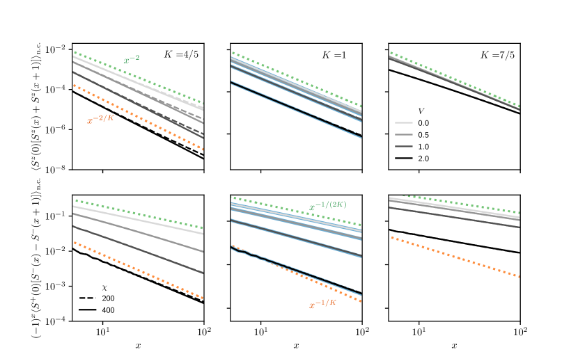
Figure 6: Correlation functions computed in $\ket{\psi_{\text{n.c.}}}$ for the $XXZ$ model using iDMRG. The upper and lower panels show respectively the $\nabla\hat{\phi}$ and $e^{i\hat{\theta}}$ correlation functions, and the Luttinger parameters $K$ vary from column to column. The different bond dimensions $\chi$ (shown dashed and solid) and measurement strengths (shades) are indicated on the legends, and are the same for all panels. Dotted lines show theoretical predictions: in the upper right panel the orange line shows the behavior $x^{-2/K}$, while green lines in the upper panels show $x^{-2}$. In the lower panels orange lines show $x^{-1/K}$, while green lines show $x^{-1/(2K)}$ (see text for details). In the central panels we compare iDMRG results (greys) with exact results for a system of $L=3\times 10^{3}$ sites with periodic boundary conditions (blue, $V$ increasing from top to bottom).

First note that with $V=0$, in which case there is no measurement and $\ket{\psi_{\text{n.c.}}}=\ket{\psi_{\text{g.s.}}}$, the power-law decays of the $\nabla\hat{\phi}$ and $e^{i\hat{\theta}}$ correlators Eq. (66) indeed match TLL theory, decaying respectively as $x^{-2}$ (upper panels) and $x^{-1/(2K)}$ (lower panels) respectively. Additionally, for $K=1$ where the measurement is a marginal perturbation, the $\nabla\hat{\phi}$ correlator is simply rescaled: For small $V$ the leading order contribution arises at second order in perturbation theory, taking the form $V^{2}x^{-2}$. The behavior of the $e^{i\hat{\theta}}$ correlation function at $K=1$ is more difficult to ascertain; our theory predicts a sharp jump from $x^{-1/(2K)}$ to $x^{-1/K}$ as $K$ is decreased through unity, but this jump is smoothed out for finite $L$ (as in the results from exact diagonalization) and for finite $\chi$ (as in the iDMRG calculations). Our focus here is on behavior in the two phases, and so we defer discussion of the critical point $K=1$ to future work.

We now discuss the behavior of the $\nabla\hat{\phi}$ correlation function for $K=4/5$ and for $K=7/5$. For $K=4/5$ the expected change in the exponent from $x^{-2}$ to $x^{-2/K}=x^{-5/2}$ is not straightforward to observe on these scales; it is nevertheless clear that the measurement-induced change in this correlation function is far more significant at smaller $K$. Most striking is the fact that, for $K=7/4$ and a measurement so strong as $V=1$, the $\nabla\hat{\phi}$ correlation function is essentially unchanged, while even for $V=2$ it clearly approaches its unperturbed value as $x$ is increased. This is precisely the behavior expected for measurements that are irrelevant in the RG sense.

The $e^{i\hat{\theta}}$ correlation function shows stronger signatures of the transition. For $K=4/5$ we expect for $V=0$ a slow decay $x^{-5/8}$, while for $V\neq 0$ we expect $x^{-5/4}$ provided we go to sufficiently large $x$. Note that the length scales required to observe this crossover increase as $V\to 0$, so it is unsurprising that the behavior $x^{-5/8}$ is only observed for the larger values of $V$. For $K=7/5$ on the other hand, although our density measurements suppress the prefactor in the phase correlations, there is as expected no visible change in the power of the decay. In summary, the results of this section demonstrate a sharp contrast in the structure of $\ket{\psi_{\text{n.c.}}}$ for $K<1$ relative to $K>1$

Appendix E Gaussian measurements

As discussed in Sec. IV, in constructing our replica field theory it is convenient to use a measurement model of the form Eq. (20). In this Appendix we discuss how $\hat{M}_{m}$ can be implemented by coupling local densities $\hat{n}(x)$ to quantum harmonic oscillators (QHOs). Focus for now on a single location in space and denote by $\hat{n}$ the density there. The position operator of the QHO is $\hat{m}$. Since in Sec. IV we are concerned with a field theory, and therefore a local Hilbert space with infinite dimension, here the operators $\hat{n}$ and $\hat{m}$ are taken to have eigenvalues with all possible real values. We denote by $\ket{n}$ and $\ket{m}$ the corresponding eigenstates, with $\hat{n}\ket{n}=n\ket{n}$ and $\hat{m}\ket{m}=m\ket{m}$.

We denote by $\omega$ the frequency of the oscillator, and $\mu$ the inverse-square oscillator length. Its mass is therefore $\mu/\omega$. The Hamiltonian of the QHO should take the form

$$\hat{H}(t)=\frac{\omega}{2\mu}\hat{\pi}^{2}+\frac{1}{2}\mu\omega\hat{m}^{2}-f(t)\hat{m}\hat{n},$$ (67)

where $\hat{\pi}$ is the momentum, with $[\hat{m},\hat{\pi}]=i$. At time $t=0$ we have $f(0)=0$ and the QHO is in its ground state. Writing the state of the system as $\ket{\psi}$, with amplitudes $\braket{n}{\psi}=\psi(n)$, the combined wavefunction $\ket{\Psi(t)}$ of QHO and system is

$$\braket{n,m}{\Psi(0)}\propto\psi(n)\exp\Big{(}-\frac{1}{4}\mu m^{2}\Big{)}$$ (68)

From $t=0$ to $t=T$ we increase the coupling to $f(T)=\mu\omega$ so that

$$\hat{H}(T)=\frac{\omega}{2\mu}\hat{\pi}^{2}+\frac{1}{2}\mu\omega(\hat{m}-\hat{n})^{2}-\frac{1}{2}\mu\omega\hat{n}^{2},$$ (69)

if this increase is adiabatic with respect to the oscillator and sudden with respect to the Luttinger liquid, then

$$\braket{n,m}{\Psi(T)}\propto\psi(n)\exp\Big{(}-\frac{1}{4}\mu[m-n]^{2}\Big{)}.$$ (70)

Performing now a projective measurement of the QHO with result $m$ modifies the amplitudes $\psi(n)$ according to

$$\psi(n)\to\psi(n)\exp\Big{(}-\frac{1}{4}\mu[m-n]^{2}\Big{)},$$ (71)

which is equivalent to the operation represented by $\hat{M}_{m}$ in Eq. (20). For the coupling between the QHO and the LL to be adiabatic with respect to the QHO, we require $T\gg\omega^{-1}$. On the other hand, for it to be sudden with respect to the LL we require $T\ll\Lambda^{-1}$, where $\Lambda$ is the UV cutoff. This implies $\omega\gg\Lambda$. In order that our measurement is weak, we also require $\mu^{-1}$ to be large relative to the variance of the particle density. Large $\omega$ and small $\mu$ imply a small mass for the QHO.

References

- Bell [1964] J. S. Bell, On the Einstein Podolsky Rosen paradox, Physics Physique Fizika 1, 195 (1964).
- Aspect et al. [1982] A. Aspect, J. Dalibard, and G. Roger, Experimental test of Bell’s inequalities using time-varying analyzers, Phys. Rev. Lett. 49, 1804 (1982).
- Bennett et al. [1993] C. H. Bennett, G. Brassard, C. Crépeau, R. Jozsa, A. Peres, and W. K. Wootters, Teleporting an unknown quantum state via dual classical and Einstein-Podolsky-Rosen channels, Phys. Rev. Lett. 70, 1895 (1993).
- Bouwmeester et al. [1997] D. Bouwmeester, J.-W. Pan, K. Mattle, M. Eibl, H. Weinfurter, and A. Zeilinger, Experimental quantum teleportation, Nature 390, 575 (1997).
- Briegel and Raussendorf [2001] H. J. Briegel and R. Raussendorf, Persistent entanglement in arrays of interacting particles, Phys. Rev. Lett. 86, 910 (2001).
- Briegel et al. [2009] H. J. Briegel, D. E. Browne, W. Dür, R. Raussendorf, and M. Van den Nest, Measurement-based quantum computation, Nat. Phys. 5, 19 (2009).
- Sachdev [2011] S. Sachdev, Quantum Phase Transitions, 2nd ed. (Cambridge University Press, 2011).
- Giamarchi [2003] T. Giamarchi, Quantum physics in one dimension (Clarendon press, 2003).
- Deutsch [2018] J. M. Deutsch, Eigenstate thermalization hypothesis, Rep. Prog. Phys. 81, 082001 (2018).
- Page [1993] D. N. Page, Average entropy of a subsystem, Phys. Rev. Lett. 71, 1291 (1993).
- Tomonaga [1950] S.-I. Tomonaga, Remarks on Bloch’s method of sound waves applied to many-fermion problems, Prog. Theor. Phys. 5, 544 (1950).
- Luttinger [1963] J. M. Luttinger, An exactly soluble model of a many-fermion system, J. Math. Phys. 4, 1154 (1963).
- Haldane [1981a] F. D. M. Haldane, Effective harmonic-fluid approach to low-energy properties of one-dimensional quantum fluids, Phys. Rev. Lett. 47, 1840 (1981a).
- Haldane [1981b] F. D. M. Haldane, 'Luttinger liquid theory' of one-dimensional quantum fluids. I. properties of the Luttinger model and their extension to the general 1d interacting spinless Fermi gas, J. Phys. C 14, 2585 (1981b).
- Schwartz et al. [1998] A. Schwartz, M. Dressel, G. Grüner, V. Vescoli, L. Degiorgi, and T. Giamarchi, On-chain electrodynamics of metallic salts: Observation of Tomonaga-Luttinger liquid response, Phys. Rev. B 58, 1261 (1998).
- Yao et al. [1999] Z. Yao, H. W. C. Postma, L. Balents, and C. Dekker, Carbon nanotube intramolecular junctions, Nature 402, 273 (1999).
- Rüegg et al. [2008] C. Rüegg, K. Kiefer, B. Thielemann, D. F. McMorrow, V. Zapf, B. Normand, M. B. Zvonarev, P. Bouillot, C. Kollath, T. Giamarchi, S. Capponi, D. Poilblanc, D. Biner, and K. W. Krämer, Thermodynamics of the spin Luttinger liquid in a model ladder material, Phys. Rev. Lett. 101, 247202 (2008).
- Lake et al. [2005] B. Lake, D. A. Tennant, C. D. Frost, and S. E. Nagler, Quantum criticality and universal scaling of a quantum antiferromagnet, Nat. Mater. 4, 329 (2005).
- Kono et al. [2015] Y. Kono, T. Sakakibara, C. P. Aoyama, C. Hotta, M. M. Turnbull, C. P. Landee, and Y. Takano, Field-induced quantum criticality and universal temperature dependence of the magnetization of a spin- Heisenberg chain, Phys. Rev. Lett. 114, 037202 (2015).
- Paredes et al. [2004] B. Paredes, A. Widera, V. Murg, O. Mandel, S. Fölling, I. Cirac, G. V. Shlyapnikov, T. W. Hänsch, and I. Bloch, Tonks-Girardeau gas of ultracold atoms in an optical lattice, Nature 429, 277 (2004).
- Kinoshita et al. [2004] T. Kinoshita, T. Wenger, and D. S. Weiss, Observation of a one-dimensional Tonks-Girardeau gas, Science 305, 1125 (2004).
- Hofferberth et al. [2008] S. Hofferberth, I. Lesanovsky, T. Schumm, A. Imambekov, V. Gritsev, E. Demler, and J. Schmiedmayer, Probing quantum and thermal noise in an interacting many-body system, Nat. Phys. 4, 489 (2008).
- Yang et al. [2017] B. Yang, Y.-Y. Chen, Y.-G. Zheng, H. Sun, H.-N. Dai, X.-W. Guan, Z.-S. Yuan, and J.-W. Pan, Quantum criticality and the Tomonaga-Luttinger liquid in one-dimensional bose gases, Phys. Rev. Lett. 119, 165701 (2017).
- Patil et al. [2014] Y. S. Patil, S. Chakram, L. M. Aycock, and M. Vengalattore, Nondestructive imaging of an ultracold lattice gas, Phys. Rev. A 90, 033422 (2014).
- Patil et al. [2015] Y. S. Patil, S. Chakram, and M. Vengalattore, Measurement-induced localization of an ultracold lattice gas, Phys. Rev. Lett. 115, 140402 (2015).
- Wiseman and Milburn [1993] H. M. Wiseman and G. J. Milburn, Quantum theory of field-quadrature measurements, Phys. Rev. A 47, 642 (1993).
- Kane and Fisher [1992a] C. L. Kane and M. P. A. Fisher, Transport in a one-channel Luttinger liquid, Phys. Rev. Lett. 68, 1220 (1992a).
- Kane and Fisher [1992b] C. L. Kane and M. P. A. Fisher, Transmission through barriers and resonant tunnelling in an interacting one-dimensional electron gas, Phys. Rev. B 46, 15233 (1992b).
- Buchhold et al. [2021] M. Buchhold, Y. Minoguchi, A. Altland, and S. Diehl, Effective theory for the measurement-induced phase transition of Dirac fermions, Phys. Rev. X 11, 041004 (2021).
- Minoguchi et al. [2022] Y. Minoguchi, P. Rabl, and M. Buchhold, Continuous Gaussian measurements of the free boson CFT: A model for exactly solvable and detectable measurement-induced dynamics, SciPost Phys. 12, 9 (2022).
- Cao et al. [2019] X. Cao, A. Tilloy, and A. D. Luca, Entanglement in a fermion chain under continuous monitoring, SciPost Phys. 7, 24 (2019).
- Li et al. [2018] Y. Li, X. Chen, and M. P. A. Fisher, Quantum Zeno effect and the many-body entanglement transition, Phys. Rev. B 98, 205136 (2018).
- Skinner et al. [2019] B. Skinner, J. Ruhman, and A. Nahum, Measurement-induced phase transitions in the dynamics of entanglement, Phys. Rev. X 9, 031009 (2019).
- Chan et al. [2019] A. Chan, R. M. Nandkishore, M. Pretko, and G. Smith, Unitary-projective entanglement dynamics, Phys. Rev. B 99, 224307 (2019).
- Li et al. [2021] Y. Li, X. Chen, A. W. W. Ludwig, and M. P. A. Fisher, Conformal invariance and quantum nonlocality in critical hybrid circuits, Phys. Rev. B 104, 104305 (2021).
- Friedman et al. [2022] A. J. Friedman, C. Yin, Y. Hong, and A. Lucas, Locality and error correction in quantum dynamics with measurement, arXiv:2206.09929 (2022).
- Li et al. [2019] Y. Li, X. Chen, and M. P. A. Fisher, Measurement-driven entanglement transition in hybrid quantum circuits, Phys. Rev. B 100, 134306 (2019).
- Bao et al. [2020] Y. Bao, S. Choi, and E. Altman, Theory of the phase transition in random unitary circuits with measurements, Phys. Rev. B 101, 104301 (2020).
- Jian et al. [2020] C.-M. Jian, Y.-Z. You, R. Vasseur, and A. W. W. Ludwig, Measurement-induced criticality in random quantum circuits, Phys. Rev. B 101, 104302 (2020).
- Turkeshi et al. [2020] X. Turkeshi, R. Fazio, and M. Dalmonte, Measurement-induced criticality in -dimensional hybrid quantum circuits, Phys. Rev. B 102, 014315 (2020).
- Alberton et al. [2021] O. Alberton, M. Buchhold, and S. Diehl, Entanglement transition in a monitored free-fermion chain: From extended criticality to area law, Phys. Rev. Lett. 126, 170602 (2021).
- Turkeshi et al. [2021] X. Turkeshi, A. Biella, R. Fazio, M. Dalmonte, and M. Schiró, Measurement-induced entanglement transitions in the quantum Ising chain: From infinite to zero clicks, Phys. Rev. B 103, 224210 (2021).
- Bao et al. [2021a] Y. Bao, S. Choi, and E. Altman, Symmetry enriched phases of quantum circuits, Ann. Phys. (Amsterdam) 435, 168618 (2021a).
- Müller et al. [2022] T. Müller, S. Diehl, and M. Buchhold, Measurement-induced dark state phase transitions in long-ranged fermion systems, Phys. Rev. Lett. 128, 010605 (2022).
- Lavasani et al. [2021] A. Lavasani, Y. Alavirad, and M. Barkeshli, Measurement-induced topological entanglement transitions in symmetric random quantum circuits, Nat. Phys. 17, 342 (2021).
- Ippoliti et al. [2021] M. Ippoliti, M. J. Gullans, S. Gopalakrishnan, D. A. Huse, and V. Khemani, Entanglement phase transitions in measurement-only dynamics, Phys. Rev. X 11, 011030 (2021).
- Van Regemortel et al. [2021] M. Van Regemortel, Z.-P. Cian, A. Seif, H. Dehghani, and M. Hafezi, Entanglement entropy scaling transition under competing monitoring protocols, Phys. Rev. Lett. 126, 123604 (2021).
- Ben-Zion et al. [2020] D. Ben-Zion, J. McGreevy, and T. Grover, Disentangling quantum matter with measurements, Phys. Rev. B 101, 115131 (2020).
- Verresen et al. [2021] R. Verresen, N. Tantivasadakarn, and A. Vishwanath, Efficiently preparing Schrödinger’s cat, fractons and non-abelian topological order in quantum devices, arXiv:2112.03061 (2021).
- Tantivasadakarn et al. [2021] N. Tantivasadakarn, R. Thorngren, A. Vishwanath, and R. Verresen, Long-range entanglement from measuring symmetry-protected topological phases, arXiv:2112.01519 (2021).
- Lin et al. [2022] C.-J. Lin, W. Ye, Y. Zou, S. Sang, and T. H. Hsieh, Probing sign structure using measurement-induced entanglement, arXiv:2205.05692 (2022).
- Lu et al. [2022] T.-C. Lu, L. A. Lessa, I. H. Kim, and T. H. Hsieh, Measurement as a shortcut to long-range entangled quantum matter, arXiv:2206.13527 (2022).
- Bao et al. [2021b] Y. Bao, M. Block, and E. Altman, Finite time teleportation phase transition in random quantum circuits, arXiv:2110.06963 (2021b).
- Nielsen and Chuang [2011] M. A. Nielsen and I. L. Chuang, Quantum Computation and Quantum Information: 10th Anniversary Edition (Cambridge University Press, 2011).
- Caldeira and Leggett [1981] A. O. Caldeira and A. J. Leggett, Influence of dissipation on quantum tunneling in macroscopic systems, Phys. Rev. Lett. 46, 211 (1981).
- Furusaki and Nagaosa [1993] A. Furusaki and N. Nagaosa, Single-barrier problem and anderson localization in a one-dimensional interacting electron system, Phys. Rev. B 47, 4631 (1993).
- Cardy [1996] J. Cardy, Scaling and Renormalization in Statistical Physics, Cambridge Lecture Notes in Physics (Cambridge University Press, 1996).
- Arute et al. [2019] F. Arute, K. Arya, R. Babbush, D. Bacon, J. C. Bardin, R. Barends, R. Biswas, S. Boixo, F. G. Brandao, D. A. Buell, et al., Quantum supremacy using a programmable superconducting processor, Nature 574, 505 (2019).
- [59] In preparation.
- Efetov [1983] K. B. Efetov, Supersymmetry and theory of disordered metals, Adv. Phys. 32, 53 (1983).
- Sandvik [2010] A. W. Sandvik, Computational studies of quantum spin systems, AIP Conf. Proc. 1297, 135 (2010).
- Gullans and Huse [2020] M. J. Gullans and D. A. Huse, Scalable probes of measurement-induced criticality, Phys. Rev. Lett. 125, 070606 (2020).
- Ippoliti and Khemani [2021] M. Ippoliti and V. Khemani, Postselection-free entanglement dynamics via spacetime duality, Phys. Rev. Lett. 126, 060501 (2021).
- Lu and Grover [2021] T.-C. Lu and T. Grover, Spacetime duality between localization transitions and measurement-induced transitions, Phys. Rev. X Quantum 2, 040319 (2021).
- Ippoliti et al. [2022] M. Ippoliti, T. Rakovszky, and V. Khemani, Fractal, logarithmic, and volume-law entangled nonthermal steady states via spacetime duality, Phys. Rev. X 12, 011045 (2022).
- Bakr et al. [2009] W. S. Bakr, J. I. Gillen, A. Peng, S. Fölling, and M. Greiner, A quantum gas microscope for detecting single atoms in a hubbard-regime optical lattice, Nature 462, 74 (2009).
- Gross and Bakr [2021] C. Gross and W. S. Bakr, Quantum gas microscopy for single atom and spin detection, Nat. Phys. 17, 1316 (2021).
- Hauschild and Pollmann [2018] J. Hauschild and F. Pollmann, Efficient numerical simulations with Tensor Networks: Tensor Network Python (TeNPy), SciPost Phys. Lect. Notes , 5 (2018), code available from https://github.com/tenpy/tenpy, arXiv:1805.00055 .
- Pollmann et al. [2009] F. Pollmann, S. Mukerjee, A. M. Turner, and J. E. Moore, Theory of finite-entanglement scaling at one-dimensional quantum critical points, Phys. Rev. Lett. 102, 255701 (2009).