The clustering properties of AGNs/quasars in CatWISE2020 catalog

Abstract

We study the clustering properties of 1,307,530 AGNs/quasars in the CatWISE2020 catalog prepared using the Wide-field Infrared Survey Explorer (WISE) and Near-Earth Object Wide-field Infrared Survey Explorer (NEOWISE) survey data. For angular moments $\ell\gtrapprox 10$ ($\lessapprox 18^{\circ}$) down to non-linear scales, the results are in agreement with the standard $\Lambda$CDM cosmology, with a galaxy bias roughly matching that of the NRAO VLA Sky Survey (NVSS) AGNs. We further explore the redshift dependence of the fraction of infrared bright AGNs on stellar mass, $f_{\rm IB}\sim M_{*}^{\alpha_{0}+\alpha_{1}z}$, and find $\alpha_{1}=1.27^{+0.25}_{-0.30}$, ruling out a non-evolution hypothesis at $\approx 4.6\sigma$ confidence level. The results are consistent with the measurements obtained with NVSS AGNs, though considerably more precise thanks to the significantly higher number density of objects in CatWISE2020. The excess dipole and high clustering signal above angular scale $\approx 18^{\circ}$ remain anomalous.

1 Introduction

Recently, Secrest et al. (2021) derived an all-sky active galactic nuclei (AGN)/quasar sample from the CatWISE2020 catalog (AGN-CatWISE2020 hereafter) and studied the large-scale anisotropy of the universe by measuring the dipole signal. They find a dipole amplitude that conflicts with the prediction of the $\Lambda$CDM at the $4.9\sigma$ level, as had been also indicated, albeit with less significance, in earlier studies of the dipole in AGN catalogs prepared using radio telescopes (Singal, 2011; Rubart & Schwarz, 2013; Tiwari et al., 2015; Tiwari & Jain, 2015; Tiwari & Nusser, 2016; Siewert et al., 2021).

The AGN-CatWISE2020 is a satellite-based catalog and presumably not affected by systematics and observational biases such as declination-dependent sensitivity or atmospheric effects present in catalogs prepared using ground-based radio surveys. However, the AGN-CatWISE2020, prepared using deep photometric measurements in the infrared band at $3.4$ and $4.6$ $\mu$m from the cryogenic, post-cryogenic, and reactivation phases of the WISE mission has its own observational systematics, such as the directional bias from uncorrected Galactic reddening, poor-quality photometry near clumpy and resolved nebulae, image artifacts near bright stars, uneven source density due to scanning overlap etc. Even so, the AGN-CatWISE2020 remains an independent AGN catalog with a completely different observational setup and instrumentation in contrast to canonical radio AGN catalogs prepared using ground-based radio telescope surveys, and thus provides the opportunity to independently study AGN spatial distribution properties and their connection to background matter density and their host halos.

Our present picture of structure formation is based on the standard $\Lambda$ cold dark matter ($\Lambda$CDM); the model describes the large-scale structure formation and its evolution successfully. The matter density of the Universe is dominated by cold dark matter, and according to the theory of gravitational instability, tiny fluctuations in the initial mass density field evolve and result in a population of virialized dark matter halos of different masses (Press & Schechter, 1974). The formation of galaxies occurs inside these dark matter halos, the host halo mass and its evolution largely decide the residing galaxy properties (White & Rees, 1978; Frenk et al., 1988; White & Frenk, 1991). The AGNs span the high mass end of the halo mass distribution and thus with AGN clustering analysis, we explore the clustering properties of relatively high mass halos. The radio emission from a galaxy and its stellar mass is known to have a close connection (Best et al., 2005; Donoso et al., 2009; Nusser & Tiwari, 2015; Sabater et al., 2019). We assume a similar connection for infared selected AGNs and further explore this connection in this work.

We follow the standard correlation function and power spectrum analysis to explore the spatial distribution of AGNs from the WISE mission and their connection to the background dark matter distribution, i.e., the galaxy bias for these AGNs. Throughout the paper, we adopt the $\Lambda$CDM model and use Planck $2018$ cosmological parameters as the fiducial cosmology. In particular, we set base cosmology parameters from Planck Collaboration et al. (2020), i.e. TT,TE,EE+lowE+lensing $\omega_{b}h^{2}=0.02237$, $\omega_{c}h^{2}=0.1200$, $100\theta_{\rm MC}=1.04092$, $\tau=0.0544$, $\ln(10^{10}A_{s})=3.044$ and $n_{s}=0.9649$.

We discuss the data and AGN selection details in Section 2. In Section 3, we briefly describe the theoretical formulation for angular power spectrum and projected two-point correlation function. Mocks data and and covariance matrix generation are detailed in Section 4. Section 5 presents the results. We conclude with discussion in Section 6.

2 CatWISE2020 catalog and AGN selection

The CatWISE2020 (Marocco et al., 2021) catalog covers the entire sky and contains 1,890,715,640 sources from the Wide-field Infrared Survey Explorer (WISE, Wright et al. 2010) and the Near-Earth Object Wide-field Infrared Survey Explorer (NEOWISE) deep photometric surveys at 3.4 and 4.6 $\mu$m (W1 and W2). The catalog is 90% complete at W1=17.7 mag and W2=17.5 mag. Relying on distinguishing the power-law spectrum of AGNs from the blackbody spectrum of galaxies and stars, the mid-infrared WISE bands W1 and W2 can reliably identify AGNs. A simple color criterion of $W1-W2\geq 0.8$ identifies both unobscured (type 1) and obscured (type 2) AGNs (Stern et al., 2012) which presumably follow their characteristic power-law ($S_{\nu}\propto\nu^{-\alpha}$). Secrest et al. (2021) apply this color criterion, i.e., $W1-W2\geq 0.8$ on CatWISE2020 catalog and find $141,698,603$ sources. They mask the nebulae in our and nearby galaxies and the bright stars (in total $291$ sky regions) to remove the poor-quality photometry regions. Also, they impose a magnitude selection cut of $9<W1<16.4$ to correct for uneven source density due to overlap in the WISE scanning pattern. Further they mask Galactic latitudes of $|b|<30^{\circ}$ and impose some additional masks and cuts (for details see Secrest et al. 2021) and produce a source catalog of $1,355,352$ sources. The source catalog thus obtained and the mask are shown, using HEALPix (Goŕski et al., 2005) Mollweide projection with NSIDE=64, in Figure 1. The catalog covers almost 50% of the sky. We note that the projected pixel count in cells shows a tail toward zero ends (Figure 3). We find this to be because of low source count at mask edges, an artifact of projection in HEALPix pixels of finite sizes. We thus additionally mask all the neighbouring pixels of masked pixels and produce an alternate mask for AGN-CatWISE2020. With this alternate mask we are left with 1,307,530 sources and around 47.25% of sky coverage. The mask and the projected source number density is shown in Figure 2. For our all analysis in this work we use this alternate mask and 1,307,530 AGNs left after applying this mask. The source count in pixels with canonical and our alternate mask is shown in Figure 3. The CatWISE catalog also shows a mild inverse linear trend in source number density versus absolute ecliptic latitude with a slope of $-0.051$ and a zero-latitude intercept of $68.89$ deg^-2(Secrest et al., 2021). We correct the number density to account for this trend. All results throughout the paper are after applying the ecliptic latitude correction.

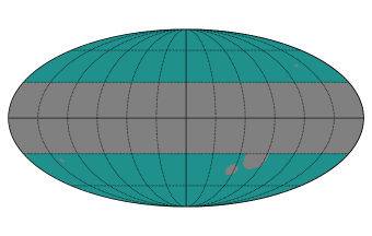
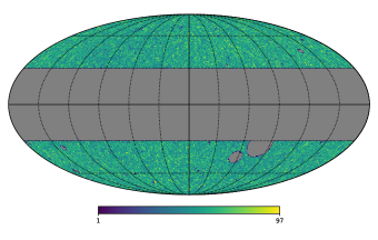
Figure 1: AGN-CatWISE2020 mask (top) and catalog by Secrest et al. (2021) in galactic coordinates. There are 1,355,352 sources in the catalog and the data cover 49.65% of the sky.

Figure 2: Alternate mask and AGN catalog after masking in galactic coordinates. We are left with 1,307,530 sources in the catalog and the data covers 47.35% of the sky.

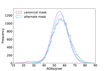
Figure 3: The source count in HEALPix pixels with NSIDE=64. The canonical mask shows a tail towards zero ends. The counts in pixels with our alternate mask are a better fit with the Poisson distribution (dashed line curves).

2.1 The redshift distribution

The photometric data from the WISE and NEOWISE do not contain redshift information. To derive an estimate for their redshift distributions, Secrest et al. (2021) cross match the catalog with SDSS strip 82 sub-region between $-42^{\circ}<$ R.A. $<45^{\circ}$, this area lies outside the AGN-CatWISE2020 mask and has been surveyed several times by SDSS and by the extended Baryon Oscillation Spectroscopic Survey (eBOSS; Dawson et al. 2016). This region also has an overlap with the Dark Energy Survey, Data Release 1 (DES1; Abbott et al. 2018) and Gaia Data Release 2 (Gaia Collaboration et al., 2018). Secrest et al. (2021) report 14,402 AGNs in this region and after correcting DES1 source positions using Gaia DR2 they find DES1 counterparts for 14,193 sources (99%). They find spectroscopic information for $\sim 61$% of the AGNs using specObj tables for SDSS DR16. The redshift distribution thus obtained is shown in Figure 4. Using DES1 and WISE photometric bands, i.e., r-W2 value Secrest et al. (2021) argue that the AGNs without SDSS spectral redshifts are faint at visual wavelengths. The matched objects may be used to represent the distribution of redshifts for the full sample. However, as this redshift PDF is prepared using spectroscopic information of only $\sim 61$% sources, considering this as reliably representing full sample remains debatable.

We therefore produce an alternative redshift template for AGN-CatWISE2020 employing the Tiered Radio Extragalactic Continuum Simulation (TRECS; Bonaldi et al. 2019). We run TRECS for sub-mJy flux limits (at 1.4GHz) and produce redshifts for flux limited data. We find that TRECS AGNs number density matches with AGN-CatWISE2020 if we consider flux density $>1.15$ mJy at 1.4 GHz. Assuming, AGN-CatWISE2020 is complete above a constant flux density, the TRECS redshifts above flux density $>1.15$ mJy at 1.4 GHz represent AGN-CatWISE2020. We have shown the redshift PDF thus obtained using TRECS in Figure 4. For comparison, we also show the PDF best fitted to NRAO VLA Sky Survey (NVSS; Condon et al. 1998) AGNs (Nusser & Tiwari, 2015). This best fit to NVSS by Nusser & Tiwari (2015) is obtained by considering the redshifts from Combined EIS-NVSS Survey of Radio Source (CENSORS) and Hercules (Rigby et al., 2011), both in total containing 165 sources above 7.5 mJy at 1.4 GHz. We have shown CENSORS+Hercules redshifts (normalized) also in same figure for comparison. We will also use this redshift distribution as an alternate template to fit CatWISE2020 AGNs considered in this work. We add that TRECS and CENSORS+Hercules represent the radio-selected AGNs and WISE-selected AGNs may have somewhat different ${N(z)}$. We employ these as optional ${N(z)}$. In any case, these redshift distributions only slightly differ from Secrest et al. (2021) (see Figure 4).

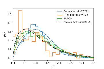
Figure 4: The redshift distribution of AGN-Catwise2020 sample by Secrest et al. (2021). We also show the best fit PDF to the NVSS AGNs with integrated flux grater than 10 mJy at 1.4 GHz and the TRECS for comparison. The best fitted (dashed lines), parameterized $N(z)\propto z^{a_{1}}\exp\left[-\left(\frac{z}{a_{2}}\right)^{a_{3}}\right]$, are also shown for different $N(z)$ templates.

3 Theoretical formulation

In the absence of redshift measurements, the angular power spectrum and angular correlation function of galaxies are standard tools for analyzing the clustering properties of galaxies and inferring information on their luminosity, biasing, and background cosmology (Magliocchetti et al., 1999; Blake & Wall, 2002; Overzier et al., 2003; Nusser & Tiwari, 2015; Hale et al., 2018; Tiwari et al., 2022). We briefly discuss these below.

3.1 Angular power spectrum

Given a uniform galaxy survey catalog with a total number of galaxies ${\cal N}$ and with angular area coverage $\mathcal{A}$, the mean number density per steradian is, $\bar{\cal N}={\cal N}/\mathcal{A}$. The projected number density in the direction $\hat{\boldsymbol{r}}$, can have the expression, ${\cal N}(\hat{\boldsymbol{r}})=\bar{\cal N}(1+\Delta(\hat{\boldsymbol{r}}))$, where $\Delta(\hat{\boldsymbol{r}})$ is the projected number density contrast and is theoretically connected to the underlying matter density contrast, $\delta_{m}(\boldsymbol{r})$. The galaxy density contrast $\delta_{g}(\boldsymbol{r})$ traces $\delta_{m}(\boldsymbol{r})$ through a bias factor, the galaxy biasing $b(z)$,

$$\delta_{g}(\boldsymbol{r})=\delta_{m}(\boldsymbol{r})b(z),$$ (1)

Note $\boldsymbol{r}$ stands for comoving distance $r$ corresponding to redshift $z$ in direction $\hat{r}$. $\Delta(\hat{\boldsymbol{r}})$ can be obtained by integrating over the radial distribution of galaxies.

$$\Delta(\hat{\boldsymbol{r}}) = \int_{0}^{\infty}\delta_{g}(\boldsymbol{r})N(z)dz$$ (2)

$$= \int_{0}^{\infty}\delta_{m}(\boldsymbol{r})b(z)N(z)dz,$$

where $N(z)\differential z$, the radial distribution function, is the probability of observing a galaxy between redshift $z$ and $(z+\differential z)$. In addition to this leading term, $\Delta(\hat{\boldsymbol{r}})$ also have tiny additional contributions from lensing, redshift distortions etc. (Chen & Schwarz, 2015). These effects are within a few percent on the largest scales (Dolfi et al., 2019). To estimate the galaxy clustering at different angular scales, we expand $\Delta(\hat{\boldsymbol{r}})$ in terms of spherical harmonics,

$$\Delta(\hat{\boldsymbol{r}})=\sum_{\ell m}{a_{\ell m}}Y_{\ell m}(\hat{\boldsymbol{r}}).$$ (3)

Using the orthonormal property of spherical harmonics, we write ${a_{\ell m}}$ as,

$${a_{\ell m}} = \int d\Omega\Delta(\hat{\boldsymbol{r}})Y_{\ell m}^{*}(\hat{\boldsymbol{r}})$$

$$= \int d\Omega Y_{\ell m}^{*}(\hat{\boldsymbol{r}})\int_{0}^{\infty}\delta_{m}(\boldsymbol{r})b(z)N(z)dz\;.$$

Next one can Fourier transform the matter density field $\delta_{m}(\boldsymbol{r})$ in terms of the $\boldsymbol{k}$-space density field $\delta_{\boldsymbol{k}}$, and write the expression for angular power spectrum, ${C_{\ell}}$, by using the definition of matter power spectrum $P(k)$, i.e. $\innerproduct{\delta_{\boldsymbol{k}}\delta_{\boldsymbol{k}^{\prime}}}{\delta_{\boldsymbol{k}}\delta_{\boldsymbol{k}^{\prime}}}=(2\pi)^{3}\delta^{D}(\boldsymbol{k}-\boldsymbol{k}^{\prime})P(k)$ (for detailed formulation see Loureiro et al. 2019; Tiwari et al. 2022 etc.),

$$C_{\ell} = <|{a_{\ell m}}|^{2}>$$ (5)

$$= \frac{2}{\pi}\int dkk^{2}W^{2}(k)P(k,z=0)\;,$$

where $W(k)$ is the $k$-space window function given by

$$W^{2}(k)=\left|\int_{0}^{\infty}dzD(z)b(z)N(z)j_{\ell}(kr)\right|^{2}$$ (6)

where $D(z,k)$ represents the growth factor with dependence on $k$ due to deviations from the linear evolution on small scales.

We use the Core Cosmology Library (CCL, Chisari et al. 2019) to calculate theoretical ${C_{\ell}}$. To derive ${C_{\ell}}$ from the masked data, we use the pseudo-$C_{\ell}$ recovery algorithm by Alonso et al. (2019). The python modules for these algorithms are publicly available as pyccl and NaMaster. Galaxies are treated as discrete point sources and hence the measured angular power spectrum of a galaxy catalog, ${C_{\ell}}^{\rm measured}$ , contains the Poissonian shot-noise equal to $\frac{1}{\bar{\cal N}}$. The ${C_{\ell}}^{\rm obs}={C_{\ell}}^{\rm measured}-\frac{1}{\bar{\cal N}}$ is equivalent to theoretical ${C_{\ell}}$ in Equation 5. The expected uncertainty in $C_{\ell}$ determination due to cosmic variance, sky coverage, and shot-noise is,

$$\Delta C_{\ell}=\left(\frac{2}{(2\ell+1)f_{\rm sky}}\right)^{1/2}C^{\rm measured}_{\ell},$$ (7)

where $f_{\rm sky}$ represents the fraction of the sky covered by the survey.

3.2 Biasing scheme for AGNs

We assume that the AGNs catalog derived from CatWISE2020 follows a biasing scheme similar to radio-loud AGNs. This assumption may not hold entirely as for the WISE selected AGNs, we only have $\sim 42\%$ radio matches (Stern et al., 2012). Nonetheless we use the same biasing scheme as for AGNs from Nusser & Tiwari (2015) and write

$$b(z)=\frac{\int^{M_{\rm max}}_{M_{\rm min}}n_{h}(M,z)b_{h}(M,z)\mathcal{F}(M_{*},z)dM}{\int^{M_{\rm max}}_{M_{\rm min}}n_{h}(M,z)\mathcal{F}(M_{*},z)dM},$$ (8)

where $n_{h}(M,z)$ is the halo number density for halos in mass range $M$ and $M+dM$ at redshift $z$, $b_{h}(M,z)$ is the bias for these halos. $\mathcal{F}(M_{*},z)$ represents the dependence of the fraction of infrared bright AGNs, $f_{IB}$, on the stellar mass $M_{*}$. We assume $f_{IB}$ to be of the form

$$f_{IB}\propto\mathcal{F}(M_{*},z)=\left(\frac{M_{*}}{10^{11}M_{\odot}}\right)^{\alpha_{0}+\alpha_{1}z}\;,$$ (9)

where $\alpha_{0}=2.5\pm 0.2$ obtained by Best et al. (2005) with local ($z<0.1$) AGNs. The parameter $\alpha_{1}$ contains the infrared brightness evolution as a function of redshift (or time). Nusser & Tiwari (2015) find $\alpha_{1}=1.85\pm 0.74$ using NVSS AGNs. For our analysis, we use HMF: Halo Mass Function calculator (Murray et al., 2013) to obtain $n_{h}(M,z)$ and $b_{h}(M,z)$, the python module of the code is publicly available as hmf.

The $M_{*}$ in equation 8 is a function of halo mass following the stellar-to-halo mass (SHM) relation from Moster et al. (2013). We choose $M_{\rm min}=4\times 10^{11}M_{\odot}$ corresponding to $M_{*}=10^{10}M_{\odot}$ which is the lowest stellar mass limit to host radio AGN (Moster et al., 2013). Considering a lower value for $M_{\rm min}$ does not make a difference due to a very steep dependence of $\mathcal{F}$ on $M_{*}$. The upper limit for the integration, i.e., $M_{\rm max}$ is set to be $10^{15}M_{\odot}$, the halos above this mass are very rare, i.e., $n_{h}(M,z)\to 0$ for $M>10^{15}M_{\odot}$.

3.3 Angular correlation function

The angular correlation function, $w(\theta)$, is a measure of galaxy clustering in angular space; an alternate to angular power spectrum discussed in Section 3.1. The two-point angular correlation function is defined as the excess probability, relative to a random distribution, of finding a pair of galaxies in both of the elements of solid angle $d\Omega_{1}$ and $d\Omega_{2}$ at angular separation $\theta$,

$$dP=\bar{\cal N}^{2}(1+w(\theta))d\Omega_{1}d\Omega_{2},$$ (10)

where $\bar{\cal N}$ is the projected mean galaxy number density. To estimate w($\theta$) we employ Landy & Szalay (1993) estimator which is based on galaxy-galaxy (DD), random-random (RR), and galaxy-random (DR) pair counts and defined as,

$$w(\theta)=\frac{DD-2DR+RR}{RR}$$ (11)

In practice, we use the TreeCorr python module by Jarvis et al. (2004) to compute $w(\theta)$ from data. We derive the theoretical estimate of $w(\theta)$ from the model ${C_{\ell}}$ according to the relation

$$w(\theta)=\frac{1}{4\pi}\sum_{l}(2l+1){C_{\ell}}P_{l}(\cos\theta),$$ (12)

where $P_{l}(x)$ are the Legendre polynomials.

4 Covariance matrix estimation and MCMC sampling

For our pipeline calibration of data systematics and errors estimation, we generate $1000$ mocks of AGN-CatWISE2020 by employing the log-normal density field simulator code FLASK (Xavier et al., 2016). We generate log-normal density fields tomographically in $35$ redshift slices ($0$ to redshift $3.5$), each with a width $\Delta z=0.1$. We neglect AGNs beyond redshift 3.5 (see Figure 4). The statistical properties (i.e. auto and cross-correlations) of mocks are determined by the input angular power spectrum that we generate using CAMB (Challinor & Lewis, 2011), including the effect of redshift-space distortions, non-linear power spectrum corrections, and lensing. For the mock generation, we assume the bias $b(z)$ and $N(z)$ distribution from Nusser & Tiwari (2015) and generate auto and cross $C_{\ell}$s using CAMB and provide inputs to FLASK to generate mock number count maps. We apply the survey mask, shown in Figure 2, to account for survey geometry. Next from the mocks, we calculate the angular power spectrum and compute the covariance matrix. To reduce noise and smooth recovery of pseudo-${C_{\ell}}$ we collect power in multipole bins by averaging over 16 multipoles. We have shown the correlation matrix of the binned angular power spectrum in Figure 5.

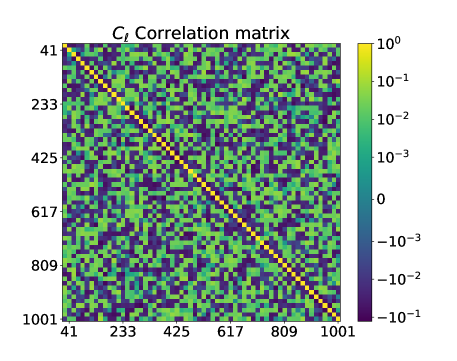
Figure 5: The angular power spectrum correlation matrix constructed from 1000 mocks generated using FLASK log-normal density simulator. Each galaxy mock follows the same sky coverage and contains approximately the same number of sources as our AGN-CatWISE2020 catalog.

We fit the AGN-CatWISE2020 angular power spectrum with standard $\Lambda$CDM and constrain the galaxy bias $b(z)$ and radial distribution $N(z)$. The likelihood, $\mathcal{L}({C^{\rm obs}_{\ell}})$, i.e., the probability to observe data ${C^{\rm obs}_{\ell}}$ given the model, $\mathcal{P}({C^{\rm obs}_{\ell}}|{b(z)},{N(z)})$ is

$$\mathcal{L}\propto\exp\left[-\frac{1}{2}(\mathbf{{C^{\rm obs}_{\ell}}}-\mathbf{{C^{\rm th}_{\ell}}})^{T}\mathbf{\Sigma^{-1}}(\mathbf{{C^{\rm obs}_{\ell}}}-\mathbf{{C^{\rm th}_{\ell}}})\right],$$ (13)

where $\mathbf{\Sigma}$ is the covariance matrix computed from the mocks discussed above. Applying Bayes’ probability theorem $P(A|B)P(B)=P(B|A)P(A)$, the model probability given the data,

$$\mathcal{P}({b(z)},{N(z)}|{C^{\rm obs}_{\ell}})=\mathcal{P}({C^{\rm obs}_{\ell}}|{b(z)},{N(z)})\times$$

$$\mathcal{P}({b(z)})\times\mathcal{P}({N(z)})\;,$$ (14)

where $\mathcal{P}({b(z)})$ and $\mathcal{P}({N(z)})$ are the prior probability of bias ${b(z)}$ and ${N(z)}$, respectively. We consider parameterised $N(z)\propto z^{a_{1}}\exp\left[-\left(\frac{z}{a_{2}}\right)^{a_{3}}\right]$ and the ${b(z)}$ as discussed in Section 3.2. The prior information for ${N(z)}$ is the redshift histograms shown in Figure 4, and for ${b(z)}$ we consider flat prior. For convenience we use Cobaya(Torrado & Lewis, 2021) to perform Bayesian analysis and CosmoMC (Lewis & Bridle, 2002; Lewis, 2013) for MCMC sampling.

5 Results

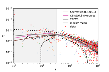
Figure 6: The angular power spectrum recovery from AGN-CatWISE2020. The open red circles are the data points with negative values (absolute value plotted). The dashed curves show the one sigma limits for the ‘TRECS’ case, calculated using equation 7. The data ${C_{\ell}}$s for $\ell\lessapprox 10$ are anomalous, showing excess power. We have reasonably good recovery above multipole $\ell\gtrapprox 30$, we only fit beyond the gray shaded area, and in this range, the mocks are a good match with the data. We have shown five random mocks (asterisks), and mocks’ mean from all 1000 mocks for illustration. The best fits with different $N(z)$ data are also shown.

We recover the pseudo-${C_{\ell}}$ from our masked AGN-CatWISE2020 (shown in Figure 2) using NaMaster (Alonso et al., 2019). The results are shown in Figure 6. We notice the excess power for multipoles, $\ell\lessapprox 10$. The recovered ${C_{\ell}}$s beyond $\ell=30$ agree well with the prediction of the standard $\Lambda$CDM cosmology. Also, the recovered pseudo-${C_{\ell}}$s show a large scatter and therefore we use band-powers defined by averaging over bins of $\Delta\ell=16$ multipoles. The results are presented in Figure 7. We consider the parameterized $N(z)\propto z^{a_{1}}\exp\left[-\left(\frac{z}{a_{2}}\right)^{a_{3}}\right]$ and the bias ${b(z)}$ as in equation 8 and run MCMC sampling over parameters $a_{1}$, $a_{2}$, $a_{3}$, $\alpha_{0}$ and $\alpha_{1}$ to find maximum likelihood values of these for observed ${C_{\ell}}$s. We assume a flat prior for ${b(z)}$ and for ${N(z)}$ we consider the redshift distribution PDF by Secrest et al. (2021). We drop the largest scale ${C_{\ell}}$s and calculate the likelihood probability for the theory power spectrum in the multipoles range $\ell=33$ to $1025$. The non-linear $\Lambda$CDM power spectrum fits the data well with $\chi^{2}/dof=1.46$. The non-linear fit is distinguishable from the linear matter power spectrum beyond $\ell\sim 250$. The likelihood contours of the parameters $\alpha_{0}$ and $\alpha_{1}$ are shown in Figure 8 with best values $\alpha_{0}=2.50^{+0.24}_{-0.19}$ and $\alpha_{1}=1.27^{+0.25}_{-0.30}$. These are consistent with (Nusser & Tiwari, 2015) within one $\sigma$ error. The best $b(z)$ values are shown in Figure 9. A quadratic function $b(z)=1.54^{+0.13}_{-0.12}+0.53^{+0.01}_{-0.01}z+0.50^{+0.03}_{-0.03}z^{2}$ represents well the bias curve and its one sigma limits. The MCMC run samples, best values of the parameters, and parameter correlations are shown in Figure 10. We add that the clustering dipole magnitude expected with this bias and $N(z)$ assuming $\Lambda$CDM is $0.81\times 10^{-3}$ (i.e. $C_{1}=0.91\times 10^{-6}$). However, notice that the dipole signal in galaxy count is largely from aberration and Doppler effects caused by local motion (Ellis & Baldwin, 1984), and for CatWISE2020 the predicted value is $0.73\times 10^{-2}$ (Secrest et al., 2022).

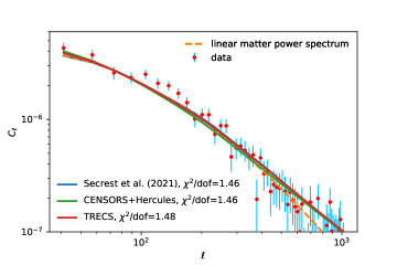
Figure 7: The angular power spectrum recovery in multipole bands, averaging over groups of $\Delta\ell$ = 16 multipoles. The best fits with different $N(z)$ data are also shown. All fits are almost the same resulting $\chi^{2}/dof\approx 1.5$. The plotted error bars are the standard deviations from 1000 mocks.

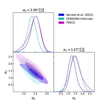
Figure 8: The best fitted $\alpha_{0}$ and $\alpha_{1}$ parameters assuming different $N(z)$ templates. The evolution parameter with $N(z)$ template from Secrest et al. (2021) is $\alpha_{1}=1.27^{+0.25}_{-0.30}$, this is $\approx 4.6\sigma$ measurement of infrared bright AGN fraction evolution.

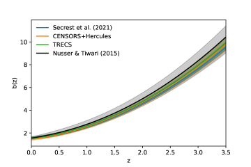
Figure 9: The best fit $b(z)$ and one $\sigma$ error bar.

We next employ redshift template produced using the TRECS simulation. We have created this template by matching the number density of AGN-CatWISE2020 and thus this arguably represents the redshifts PDF for the full sample. The TRECS redshifts fit the data well and we find $\chi^{2}/dof=1.48$. The fit to angular power spectrum is shown in Figure 7. We find slightly higher bias, $b(z)$, with TRECS (shown in Figure 9), even so the bias values remains consistent with Nusser & Tiwari (2015).

We also consider redshift distribution from CENSORS and Hercules. The CENSORS survey is over 6 deg², and the Hercules is over 1.2 deg² both in total contain 165 sources above 7.5 mJy at 1.4 GHz. These surveys are presumably complete above 7.5 mJy at 1.4 GHz. The same redshifts were used to fit angular power spectrum from NVSS (Nusser & Tiwari, 2015). This $N(z)$ also fits the data equally well, $\chi^{2}/dof=1.46$, with bias $b(z)$ slightly lower in comparison to the TRECS case.

Figure 10: The MCMC samples and results assuming Secrest et al. (2021) $N(z)$.

The angular two-point correlation function represents the angular clustering measure in real space. We use the TreeCorr (Jarvis et al., 2004) python module and calculate angular correlation function $w(\theta)$, the results are in Figure 11. We also plot the theoretical $w(\theta)$ obtained employing equation 12 and the best ${C_{\ell}}$ curves shown in Figure 7. The theoretical $w(\theta)$ plots show a reasonable match with data for scales corresponding to our multipoles fit range, i.e. $\ell<1025$ ($\theta\gtrapprox 0.18^{\circ}$). At scales below $0.1^{\circ}$ the best fit curves are moderately below the data points indicating slightly high clustering at very small scales.

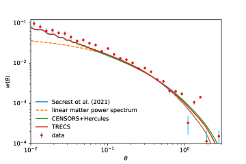
Figure 11: Angular two-point correlation function from AGN-CatWISE2020 and the theoretical fits. The fits are drawn using the best fit bias $b(z)$, and $N(z)$ obtained by fitting ${C_{\ell}}$s .

6 Discussion and Conclusion

We have examined the angular clustering of the AGNs in CatWISE2020 catalog. The angular power spectrum multipoles below $\ell\lessapprox 10$ are anomalous, with ${C_{\ell}}$s that are systematically higher than the predictions of the $\Lambda$CDM. Nonetheless, the ${C_{\ell}}$s beyond $\ell\gtrapprox 30$ are in excellent agreement with the standard cosmology and we only use the ${C_{\ell}}$s beyond $\ell>30$ to fit and obtain our results. Our analysis and results thus are independent of high dipole and quadrupole and any other systematics at the largest scales. We reduce the measurements variance by binning the power spectrum, and average over groups of $\Delta\ell=16$ multipoles, for a smooth recovery of angular ${C_{\ell}}$s. For error estimates we generated $1000$ mocks using FLASK (Xavier et al., 2016) and generate covariance matrix.

We adopt three redshift distribution templates and run MCMC to obtain the AGN clustering bias factor as a function of redshift ${b(z)}$. In particular, we use a ${N(z)}$ prior information from Secrest et al. (2021), CENSORS+Hercules (Rigby et al., 2011; Nusser & Tiwari, 2015; Tiwari & Nusser, 2016), and TRECS (Bonaldi et al., 2019). The ${N(z)}$ from Secrest et al. (2021) and CENSORS+Hercules represent partial redshifts for AGN-CatWISE2020 sample and could be closely representing the redshifts distribution for the full sample too. Assuming the AGN-CatWISE2020 contains the radio bright AGNs, we run TRECS simulations to produce redshifts. This probably represents the redshifts for the full AGN-CatWISE2020 sample. We find that all three ${N(z)}$ considered fit the data equally well producing $\chi^{2}/dof\approx 1.5$ with slightly different bias ${b(z)}$. Therefore, the angular power spectrum fails to break the degeneracy between ${b(z)}$ and ${N(z)}$, it effectively constrains only the combination of ${b(z)}$ and ${N(z)}$.

We further explore the non-linear region of structure formation with AGN-CatWISE2020. The multipoles above $\ell\gtrapprox 250$ show a better match with the non-linear in comparison to the linear background matter power spectrum. With two-point correlation plot the difference between linear and non-linear power spectrum is clearly visible (Figure 11). At smallest scales the theoretical curves with non-linear power spectrum are clearly a better fit.

Remarkably, the AGN bias ${b(z)}$ observed with NVSS (radio-selected) power spectrum in the linear regime of angular power spectrum $\ell\leq 100$, agrees within its one sigma limit with AGNs in CatWISE2020 infrared-selected sample, for liner and non-linear ($\ell\gtrapprox 250)$ regimes. Although, we obtain slightly smaller bias for infrared-selected AGNs. This consistent with the results obtained by Hickox et al. (2009). However, note that the extracted bias value depends on $N(z)$ being assumed, and we expect to be more certain about bias values once we have better redshift measurements.

We also explore the infrared brightness dependence of AGNs on star formation by considering the the radio luminosity dependence on stellar mass. Adopting the form $f_{\rm IB}\sim M_{*}^{\alpha_{0}+\alpha_{1}z}$ for the fraction of infrared bright galaxies versus stellar mass, we measure the evolution parameter, $\alpha_{1}$. Assuming a prior ${N(z)}$ from Secrest et al. (2021), we derive $\alpha_{1}=1.27^{+0.25}_{-0.30}$. Slightly larger values, $\alpha_{1}=1.45\pm 0.38$ and $1.48\pm 0.28$ are obtained with ${N(z)}$ priors from CENSORS+Hercules and TRECS, respectively. It is interesting to note that the biasing scheme and ${N(z)}$ of radio-selected AGNs work for infrared AGNs clustering signal. There may be some alternatives to biasing scheme formulation, nevertheless, the resultant ${b(z)}$ shown in Figure 9 is robust and immune to biasing schemes. A quadratic bias $b(z)=1.54+0.53z+0.50z^{2}$ conveniently represent the best bias for CatWISE2020 AGNs.

We also calculate angular two point correlation function from data and obtain reasonable recovery up to a few degrees. The theoretical curves obtained from ${C_{\ell}}$s, are a good match to data. The angular distribution of AGNs from CatWISE2020 above multipole $\ell\gtrapprox 10$ is smooth and a reasonable fit with standard cosmology.

7 Acknowledgments

We thank Subir Sarkar and Sebastian von Hausegger for providing the redshifts distribution prepared in Secrest et al. (2021). PT acknowledges the support of the RFIS grant (No. 12150410322) by the National Natural Science Foundation of China (NSFC). GBZ is supported by the National Key Basic Research and Development Program of China (No. 2018YFA0404503), NSFC Grants 11925303 and 11720101004. This research is supported by a grant from the Israeli Science Foundation grant number 936/18 and the Technion Asher Space Research Institute.

References

- Abbott et al. (2018) Abbott, T. M. C., Abdalla, F. B., Allam, S., et al. 2018, ApJ. S, 239, 18, doi: 10.3847/1538-4365/aae9f0
- Alonso et al. (2019) Alonso, D., Sanchez, J., & Slosar, A. 2019, Mon. Not. Roy. Astron. Soc., 484, 4127, doi: 10.1093/mnras/stz093
- Best et al. (2005) Best, P. N., Kauffmann, G., Heckman, T. M., et al. 2005, Monthly Notices of the Royal Astronomical Society, 362, 25, doi: 10.1111/j.1365-2966.2005.09192.x
- Blake & Wall (2002) Blake, C., & Wall, J. 2002, MNRAS, 329, L37, doi: 10.1046/j.1365-8711.2002.05163.x
- Bonaldi et al. (2019) Bonaldi, A., Bonato, M., Galluzzi, V., et al. 2019, Mon. Not. Roy. Astron. Soc., 482, 2, doi: 10.1093/mnras/sty2603
- Challinor & Lewis (2011) Challinor, A., & Lewis, A. 2011, Physical Review D., 84, 043516, doi: 10.1103/PhysRevD.84.043516
- Chen & Schwarz (2015) Chen, S., & Schwarz, D. J. 2015, Physical Review D., 91, 043507, doi: 10.1103/PhysRevD.91.043507
- Chisari et al. (2019) Chisari, N. E., Alonso, D., Krause, E., et al. 2019, ApJ. S, 242, 2, doi: 10.3847/1538-4365/ab1658
- Condon et al. (1998) Condon, J. J., Cotton, W. D., Greisen, E. W., et al. 1998, AJ, 115, 1693, doi: 10.1086/300337
- Dawson et al. (2016) Dawson, K. S., Kneib, J.-P., Percival, W. J., et al. 2016, AJ, 151, 44, doi: 10.3847/0004-6256/151/2/44
- Dolfi et al. (2019) Dolfi, A., Branchini, E., Bilicki, M., et al. 2019, A&A, 623, A148, doi: 10.1051/0004-6361/201834317
- Donoso et al. (2009) Donoso, E., Best, P. N., & Kauffmann, G. 2009, MNRAS, 392, 617, doi: 10.1111/j.1365-2966.2008.14068.x
- Ellis & Baldwin (1984) Ellis, G. F. R., & Baldwin, J. E. 1984, MNRAS, 206, 377
- Frenk et al. (1988) Frenk, C. S., White, S. D. M., Davis, M., & Efstathiou, G. 1988, ApJ, 327, 507, doi: 10.1086/166213
- Gaia Collaboration et al. (2018) Gaia Collaboration, Brown, A. G. A., Vallenari, A., et al. 2018, A&A, 616, A1, doi: 10.1051/0004-6361/201833051
- Gibelyou & Huterer (2012) Gibelyou, C., & Huterer, D. 2012, MNRAS, 427, 1994, doi: 10.1111/j.1365-2966.2012.22032.x
- Goŕski et al. (2005) Goŕski, K., Hivon, E., Banday, A., et al. 2005, ApJ, 622, 759, doi: 10.1086/427976
- Hale et al. (2018) Hale, C. L., Jarvis, M. J., Delvecchio, I., et al. 2018, MNRAS, 474, 4133, doi: 10.1093/mnras/stx2954
- Hickox et al. (2009) Hickox, R. C., Jones, C., Forman, W. R., et al. 2009, ApJ, 696, 891, doi: 10.1088/0004-637X/696/1/891
- Jarvis et al. (2004) Jarvis, M., Bernstein, G., & Jain, B. 2004, Monthly Notices of the Royal Astronomical Society, 352, 338, doi: 10.1111/j.1365-2966.2004.07926.x
- Landy & Szalay (1993) Landy, S. D., & Szalay, A. S. 1993, ApJ, 412, 64, doi: 10.1086/172900
- Lewis (2013) Lewis, A. 2013, Phys. Rev., D87, 103529, doi: 10.1103/PhysRevD.87.103529
- Lewis & Bridle (2002) Lewis, A., & Bridle, S. 2002, Phys. Rev., D66, 103511, doi: 10.1103/PhysRevD.66.103511
- Loureiro et al. (2019) Loureiro, A., Moraes, B., Abdalla, F. B., et al. 2019, MNRAS, 485, 326, doi: 10.1093/mnras/stz191
- Magliocchetti et al. (1999) Magliocchetti, M., Maddox, S. J., Lahav, O., & Wall, J. V. 1999, MNRAS, 306, 943, doi: 10.1046/j.1365-8711.1999.02596.x
- Marocco et al. (2021) Marocco, F., Eisenhardt, P. R. M., Fowler, J. W., et al. 2021, ApJ. S, 253, 8, doi: 10.3847/1538-4365/abd805
- Moster et al. (2013) Moster, B. P., Naab, T., & White, S. D. M. 2013, MNRAS, 428, 3121, doi: 10.1093/mnras/sts261
- Murray et al. (2013) Murray, S. G., Power, C., & Robotham, A. S. G. 2013, Astronomy and Computing, 3, 23, doi: 10.1016/j.ascom.2013.11.001
- Nusser & Tiwari (2015) Nusser, A., & Tiwari, P. 2015, ApJ, 812, 85, doi: 10.1088/0004-637X/812/1/85
- Overzier et al. (2003) Overzier, R. A., Röttgering, H. J. A., Rengelink, R. B., & Wilman, R. J. 2003, A&A, 405, 53, doi: 10.1051/0004-6361:20030527
- Planck Collaboration et al. (2020) Planck Collaboration, Aghanim, N., Akrami, Y., et al. 2020, A&A, 641, A6, doi: 10.1051/0004-6361/201833910
- Press & Schechter (1974) Press, W. H., & Schechter, P. 1974, ApJ, 187, 425, doi: 10.1086/152650
- Rigby et al. (2011) Rigby, E. E., Best, P. N., Brookes, M. H., et al. 2011, Monthly Notices of the Royal Astronomical Society, 416, 1900, doi: 10.1111/j.1365-2966.2011.19167.x
- Rubart & Schwarz (2013) Rubart, M., & Schwarz, D. J. 2013, A&A, 555, doi: 10.1051/0004-6361/201321215
- Sabater et al. (2019) Sabater, J., Best, P. N., Hardcastle, M. J., et al. 2019, A&A, 622, A17, doi: 10.1051/0004-6361/201833883
- Secrest et al. (2022) Secrest, N., von Hausegger, S., Rameez, M., Mohayaee, R., & Sarkar, S. 2022. https://arxiv.org/abs/2206.05624
- Secrest et al. (2021) Secrest, N. J., von Hausegger, S., Rameez, M., et al. 2021, ApJL, 908, L51, doi: 10.3847/2041-8213/abdd40
- Siewert et al. (2021) Siewert, T. M., Schmidt-Rubart, M., & Schwarz, D. J. 2021, A&A, 653, A9, doi: 10.1051/0004-6361/202039840
- Singal (2011) Singal, A. K. 2011, ApJL, 742, L23, doi: 10.1088/2041-8205/742/2/L23
- Stern et al. (2012) Stern, D., Assef, R. J., Benford, D. J., et al. 2012, ApJ, 753, 30, doi: 10.1088/0004-637X/753/1/30
- Tiwari & Jain (2015) Tiwari, P., & Jain, P. 2015, MNRAS, 447, 2658, doi: 10.1093/mnras/stu2535
- Tiwari et al. (2015) Tiwari, P., Kothari, R., Naskar, A., Nadkarni-Ghosh, S., & Jain, P. 2015, Astroparticle Physics, 61, 1, doi: 10.1016/j.astropartphys.2014.06.004
- Tiwari & Nusser (2016) Tiwari, P., & Nusser, A. 2016, Journal of Cosmology and Astroparticle Physics, 2016, 062, doi: 10.1088/1475-7516/2016/03/062
- Tiwari et al. (2022) Tiwari, P., Zhao, R., Zheng, J., et al. 2022, Astrophys. J., 928, 38, doi: 10.3847/1538-4357/ac5748
- Torrado & Lewis (2021) Torrado, J., & Lewis, A. 2021, JCAP, 2021, 057, doi: 10.1088/1475-7516/2021/05/057
- White & Frenk (1991) White, S. D. M., & Frenk, C. S. 1991, ApJ, 379, 52, doi: 10.1086/170483
- White & Rees (1978) White, S. D. M., & Rees, M. J. 1978, MNRAS, 183, 341, doi: 10.1093/mnras/183.3.341
- Wright et al. (2010) Wright, E. L., Eisenhardt, P. R. M., Mainzer, A. K., et al. 2010, AJ, 140, 1868, doi: 10.1088/0004-6256/140/6/1868
- Xavier et al. (2016) Xavier, H. S., Abdalla, F. B., & Joachimi, B. 2016, Mon. Not. Roy. Astron. Soc., 459, 3693, doi: 10.1093/mnras/stw874