Supersymmetry on the lattice: Geometry, Topology, and Spin Liquids

Abstract

In quantum mechanics, supersymmetry (SUSY) posits an equivalence between two elementary degrees of freedom, bosons and fermions. Here we show how this fundamental concept can be applied to connect bosonic and fermionic lattice models in the realm of condensed matter physics, e.g., to identify a variety of (bosonic) phonon and magnon lattice models which admit topologically nontrivial free fermion models as superpartners. At the single-particle level, the bosonic and the fermionic models that are generated by the SUSY are isospectral except for zero modes, such as flat bands, whose existence is undergirded by the Witten index of the SUSY theory. We develop a unifying framework to formulate these SUSY connections in terms of general lattice graph correspondences and discuss further ramifications such as the definition of supersymmetric topological invariants for generic bosonic systems. Notably, a Hermitian form of the supercharge operator, the generator of the SUSY, can itself be interpreted as a hopping Hamiltonian on a bipartite lattice. This allows us to identify a wide class of interconnected lattices whose tight-binding Hamiltonians are superpartners of one another, or can be derived via squaring or square-rooting their energy spectra all the while preserving band topology features. We introduce a five-fold way symmetry classification scheme of these SUSY lattice correspondences, including cases with a non-zero Witten index, based on a topological classification of the underlying Hermitian supercharge operator. These concepts are illustrated for various explicit examples including frustrated magnets, Kitaev spin liquids, and topological superconductors.

I Introduction

Supersymmetry (SUSY) has set foot into condensed matter physics in several isolated areas, beginning with disorder [1], then in the study of strongly interacting theories [2, 3, 4, 5, 6], and recently with the advent of topological mechanics [7, 8, 9, 10, 11, 12, 13, 14, 15, 16]. Some of this work parallels high energy physics, which also aims for insights into strongly interacting field theories [17, 18, 19], and to produce fermionic theories from bosonic ones. There, together with a certain level of naturalness, SUSY has gained prominence by going beyond being a mere trick and providing a leading theory of physics beyond the standard model [20]. There is, however, no analogous vision in condensed matter. But topological mechanics suggests one: SUSY may allow us to add locality to the classification of condensed matter by (conventional) symmetry and topology [21].

Topological mechanics arose from recognizing that balls-and-springs models admit a Dirac-like ‘square rooting’ connection to fermionic systems [7]. The common practice of Maxwell counting in these mechanical systems, the difference between the number of degrees of freedom and the number of constraints, turns out [7, 22] to be a determination of the Witten index [23] for these problems pointing to an underlying SUSY connection [15]. Practitioners immediately adopted this discovery, working out many linear theories with free fermion partners [8, 10, 24, 25, 11, 12, 13, 26, 27, 28, 9, 29, 30, 15], complete with topological invariants protecting zero modes in bosonic systems. They get around the absence of topologically protected zero modes in free bosonic systems [31] by using local constraints. Topology is then the preservation of zero modes provided the number of constraints do not change. If they add more constraints to the theory, they lose the zero modes. They have even shown that this topology protects the zero modes at the non-linear level [32]. So we now have mechanical systems with topological zero modes protected by local constraints due to the mere existence of their SUSY partners.

Practitioners envision most of their examples of topological mechanics as engineered metamaterials. But locality is a property of physical systems that arises naturally. Consider frustrated magnets which offer a striking example where residual entropy arises in underconstrained constrained systems. This has been seminally established by Maxwell constraint counting in geometrically frustrated systems such as the classical kagome or pyrochlore antiferromagnets [33, 34]. While such residual degeneracies in frustrated magnets are commonly referred to as accidental, as there is no apparent symmetry protection, the similarity to concepts in topological mechanics has led some of us to explore their stability in the presence of distortions or disorder [35]. What was found is that the robustness of accidental degeneracies can intimately be linked to the preservation of locality – certain types of distortions and disorder do not lift the frustration if limited to nearest neighbor interactions, effectively keeping the number of local constraints unaltered, but they resolve the degeneracies if second-neighbor interactions are included. Thus in real kagome antiferromagnets like Cs₂ZrCu₃F₁₂ or Cs₂CeCu₃F₁₂, it is the exponential fall-off of exchange constants away from nearest neighbors that seems to produce topologically protected low energy modes [35]. Stepping back one might be tempted to think of the formation of these accidental degeneracies in frustrated magnets, in analogy to topological mechanics, as the consequence of a hidden SUSY – a perspective that we will explore in this paper.

If we view topological mechanics as a vision for ‘symmetry+topology+locality’, what we know so far is that the classification of locally constrained systems is also much richer than the classification without locality. The classes in the ten-fold way of electronic band theory [36, 21] obey a periodicity in the dimension of the system: If a topological invariant exists in dimension $d$, it either exists in dimension $d+8$ for some classes or $d+2$ for others [37, 38, 39, 40]. These invariants are either ${\mathbb{Z}}$ or ${\mathbb{Z}}_{2}$ valued. Such a classification can be extended to finite frequency topological modes of bosonic systems [26, 41, 42, 16], but not to zero-frequency bosonic modes. Classifying the rigidity matrices in topological mechanics has also led to a table of invariants, but these depend on both spatial dimension $d$ and the Maxwell counting index $\nu$. While only a three-fold way exists in this case [43, 41], the periodicity and invariants of the ten-fold way is observed for $\nu=0$ but not for other values of $\nu$. No periodicity arises in the $\nu\neq 0$ regime, and it includes new invariants such as ${\mathbb{Z}}_{2}\times{\mathbb{Z}}_{2}$, ${\mathbb{Z}}_{12}$, ${\mathbb{Z}}_{15}$, ${\mathbb{Z}}_{24}$, and ${\mathbb{Z}}_{24}\times{\mathbb{Z}}_{3}$. This broader classification can be understood by realizing the existence of an underlying SUSY where the rigidity matrices act as SUSY charges – as we explain in this paper. So, including locality in the structure of topological phases appears to open the door to discovery and control of new unexpected low energy modes in condensed matter.

In this paper, we develop a unifying SUSY framework that uses locality as principal ingredient to bridge concepts from topological mechanics to frustrated magnetism. This framework evolves around a mapping between lattice models of free fermions and bosons – the most elementary description of condensed matter systems (Section II). The mapping is based on a general graph construction that provides both a visual and algebraic understanding of the underlying SUSY connection. It allows us to explore the relationship between SUSY, topology, and locality for many examples, which include, (i) fundamental connections between some of the most widely studied lattice geometries such as the kagome and honeycomb lattices (discussed in the next section) or the pyrochlore and diamond lattices (Section III), (ii) the construction of mechanical analogs of Kitaev spin liquids (Section IV), or (iii) a correspondence between degenerate coplanar spin spiral states and Fermi surfaces (Section III.2). On a conceptual level, the framework allows for the formulation of topogical invariants for non-interacting bosonic systems via their fermionic SUSY partners (Section II.4 and IV.1) and through these invariants, points a way to discovery and control of unexpected low energy modes in solid state physics.

II Supersymmetric lattice models

We can begin our way towards supersymmetry by discussing a basic property of block matrices. By squaring a Hermitian matrix of the form

$${\bf H}=\begin{pmatrix}&{\bf R}\\ {\bf R}^{\dagger}&\end{pmatrix},$$ (1)

with a generic matrix ${\bf R}$ of arbitrary dimensions, one obtains a block-diagonal matrix with two diagonal blocks

$${\bf H}^{2}=\begin{pmatrix}{\bf RR^{\dagger}}&\\ &{\bf R^{\dagger}R}\end{pmatrix}\,,$$ (2)

in which the two blocks ${\bf RR^{\dagger}}$ and ${\bf R^{\dagger}R}$ are isospectral except for zero modes which result from a potential dimension mismatch between the kernel of ${\bf R}$ and ${\bf R}^{\dagger}$ if ${\bf R}$ is not a square matrix. It will be this simple matrix relation upon which we will build our supersymmetric lattice construction in the following.

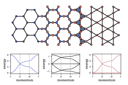
Figure 1: SUSY lattice model correspondence. Shown are three lattice geometries, the honeycomb (left, blue), honeycomb-X (middle, black), and kagome (right, red) lattices and their respective tight-binding band structures in the lower row. The honeycomb and kagome spectra are isospectral up to an additional flat band in the kagome model. The band structure of the honeycomb-X model (middle panel) can be related to the other two via squaring (or, vice versa, taking a square root). As such, the three spectra can be connected via the matrix correspondence (2), where one identifies the honeycomb and kagome lattices as supersymmetric (SUSY) partners and the honeycomb-X lattice with the SUSY charge. For the topological classification according to Table 1, we find, noting that the Witten index here is $\nu=1$, that the nexus point in the SUSY charge spectrum has a non-trivial topological invariant given by $\pi_{1}=+1$, see also the illustration in Fig. 23 of the Appendix.

To do so, let us consider the instructive example visualized in Fig. 1, which makes a connection between the familiar honeycomb lattice (on the left, blue) and the kagome lattice (on the right, red). If one calculates the band structures of their respective tight-binding Hamiltonians, e.g., by diagonalizing their nearest-neighbor hopping or graph adjacency matrices, one ends up with the two spectra plotted in the left and right panels of the lower row. These spectra are identical – up to a flat band in the kagome band structure. That is, we find an isospectrality akin to what we have seen for the matrix correspondence (2), which leads us to identify the two blocks ${\bf RR^{\dagger}}$ and ${\bf R^{\dagger}R}$ in (2) with the tight-binding Hamiltonians of the two lattices at hand. The additional flat band, or zero mode, in the kagome spectrum can then be traced back to the difference in the dimensions of the two blocks, which is simply the difference in number of sites (three) in the kagome lattice unit cell versus the two sites of the honeycomb lattice unit cell. That is, we could infer the entire spectrum of the kagome tight-binding model from the one of the honeycomb lattice without any actual calculation.

From a more abstract point of view, which we will lay out in the following, the matrix correspondence (2) allows one to identify a SUSY theory with a pair of Hamiltonians which are mandated to be isospectral and where the additional zero modes arise from a non-trivial Witten index [23]. In this sense, we have just connected the honeycomb and kagome lattices as supersymmetric partners. One could, for instance, adorn the honeycomb lattice with non-interacting fermions – the textbook example of the graphene band structure with its Dirac cone, while placing non-interacting bosonic modes on the kagome lattice – as one routinely considers in the context of studying the frustrated Heisenberg antiferromagnet on this lattice [44, 45, 46, 47], thereby pointing towards a SUSY connection between the two seemingly different worlds of Dirac semi-metals and ground-state manifolds of frustrated magnets.

In the following, we provide a more systematic understanding of the matrix correspondence (2) in terms of SUSY. When this SUSY matrix correspondence is applied to pairs of fermionic and bosonic lattice models, this perspective naturally leads one to discuss the consequences of band structure topology on the fermionic side (routinely considered, e.g., for electronic spectra) for the bosonic counterpart. On the level of the associated Bloch wavefunctions, we show that this allows one to define, for bosonic systems, a supersymmetric extension of the conventional Berry connection and curvature (or more generally, the quantum metric). Once this formal framework is established, we will recast the matrix squaring of (2) and its underlying SUSY relation of lattice models in the general terms of graph theory. This ultimately enables us to make statements on the nature of SUSY that are strikingly pictorial in that they are simple graph substitution rules.

Our SUSY framework allows us to explicate other prescriptions in the literature of squaring and square-rooting fermionic band structures [48, 41, 49, 50, 51, 52]. One important result is that the generator of the SUSY itself can be interpreted as a square-root Hamiltonian derived from the adjacency matrices of certain types of lattice graphs (and as such has a graph representation itself), while the supersymmetric partner Hamiltonians are the squared systems. In our introductory example, it is the honeycomb-X lattice  in the middle of Fig. 1 that corresponds to this SUSY generator. Its spectrum exhibits not only a flat band in the middle of its particle-hole symmetric spectrum (inherited from sqaure-rooting the flat-band kagome spectrum) but also a Dirac cone right at this particle-hole symmetric point (which it inherits from the quadratic band minima of the lowest dispersive bands in the honeycomb/kagome band structures). It is for the observation of such remarkable features, that such square-root band structures have attracted interest in the construction of lattice models for ‘square-root semimetals’ [51] or ‘square-root topological insulators’ [48, 41, 49, 50, 52].

II.1 Supersymmetry

To set the stage, let us provide a more formal introduction to how SUSY can be used to connect elementary fermionic and bosonic degrees of freedom as well as non-interacting systems of many such degrees of freedom. With an eye towards the topological classification of such non-interacting systems we then discuss how certain antiunitary symmetries, particularly relevant to the classification of free-fermion systems, transform under SUSY. This allows us to inspect topological invariants and their generalizations in supersymmetric settings.

Let us consider a system consisting of both complex fermionic and bosonic degrees of freedom. The central object that enables a supersymmetric identification between such fermions and bosons is a fermion-odd supercharge operator

$$\mathcal{Q}=c^{\dagger}{\bf R}b\,,$$ (3)

where $c^{\dagger}$ denotes a fermionic creation operator, $b$ a bosonic annihilation operator, and $Q$ satisfies $Q^{2}=0$. With this supercharge operator at hand, one can now generate a SUSY Hamiltonian via

$$\mathcal{H}_{\text{SUSY}}=\{\mathcal{Q},\mathcal{Q}^{\dagger}\} =c^{\dagger}{\bf RR^{\dagger}}c+b^{\dagger}{\bf R^{\dagger}R}b$$

$$\equiv\begin{pmatrix}c^{\dagger}&b^{\dagger}\end{pmatrix}\begin{pmatrix}{\cal H}_{F}&\\ &{\cal H}_{B}\end{pmatrix}\begin{pmatrix}c\\ b\end{pmatrix}\,.$$ (4)

From this, the two matrices, ${\bf RR^{\dagger}}$ and ${\bf R^{\dagger}R}$, which constitute the two diagonal blocks of ${\bf H}^{2}$ in (2), can be readily identified as a free fermionic and a free bosonic Hamiltonian matrix, respectively.

For a square matrix ${\bf R}$, ${\cal H}_{F}$ and ${\cal H}_{B}$ are entirely isospectral (including potential zero modes if any). For a rectangular matrix ${\bf R}$, however, there will always be a mismatch in the number of zero eigenvalues which we can characterize by the index

$$\nu ={\rm dim}({\rm kernel}[{\bf R}])-{\rm dim}({\rm kernel}[{\bf R}^{\dagger}])$$

$$={\rm col}[{\bf R}]-{\rm row}[{\bf R}]\,,$$ (5)

called the Maxwell-Calladine index in topological mechanics [7]. In the many-body problem, it is the one-body sector of the Witten index [23] $\mathrm{Tr}\,(-1)^{F}\equiv\mathrm{Tr}\,e^{i\pi c^{\dagger}c}$, and so is a topological invariant of a free SUSY theory. So long as $\nu\neq 0$, this implies SUSY can exist in the ground state. When $\nu=0$, no zero modes can exist on either side. Further, the situation for $\nu\neq 0$ is a definitive indication of flat bands to appear in the band structure of either ${\cal H}_{F}$ ($\nu<0$) and ${\cal H}_{B}$ ($\nu>0$). For example, the Witten index is $\nu=1$ for the honeycomb-kagome correspondence highlighted in the introduction which therefore has to give rise to a flat band in the kagome band structure as discussed before.

II.2 Lattice graphs

In more abstract terms, one can identify the hopping matrices of Eq. (II.1) with a (weighted) adjacency matrix of an underlying graph structure. For some lattice graph with vertices $\{v_{i}\}$ an adjacency matrix is defined as

$$\mathbf{A}_{ij}=\begin{cases}1\quad v_{i}\text{ connected to }v_{j}\\ 0\quad\text{otherwise}\,.\end{cases}$$ (6)

The weighted adjacency matrix extends this definition by including a weight $w_{ij}$ for every non-zero element of $\mathbf{A}_{ij}$.

Squaring graphs

What happens when we square an adjacency matrix $\mathbf{A}$? To find out, let us compute the elements of the squared matrix

$$(\mathbf{A}^{2})_{ik}=\sum_{j}\mathbf{A}_{ij}\mathbf{A}_{jk}\,,$$ (7)

which we can readily interpret as elements of another adjacency matrix, but with a different set of connections. Where $\mathbf{A}$ connected vertices $v_{i}$ and $v_{j}$ with weight $A_{ij}$, $\mathbf{A}^{2}$ chains two of those connections together to connect next-nearest neighboring vertices $v_{i}$ and $v_{k}$. So on a pictorial level, squaring an adjacency matrix is equivalent to singling out next-nearest neighbors of the original graph in a new graph.

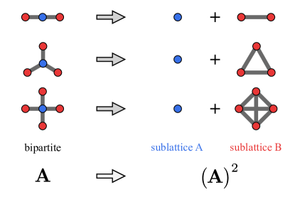
Figure 2: Squaring graphs. By squaring the (weighted) adjacency matrix $\mathbf{A}$ of a given graph, one can arrive at a squared graph by interpreting $\mathbf{A}^{2}$ as its adjacency matrix. For a given bipartite graph, this squaring gives an off-diagonal block matrix [as in (1)], which in its graph theoretical representation is equivalent to a decomposition in its two subgraphs. This process can be reversed to a ‘graph square rooting’ procedure by going from right to left in the figure, which, in the graph theoretical representation, amounts to a substitution of graph cliques of size $z$ (i.e., fully connected plaquettes with $z$ sites) by $z$-connected sites.

These statements can be further refined if $\mathbf{A}$ describes the adjacency of a bipartite graph. In this case, the matrix itself can be brought into a two-block structure upon sorting the vertices $\{v_{i}\}$ of the original bipartite graph into two distinct sets $\{v_{i}^{\rm I}\}$ and $\{v_{i}^{\rm II}\}$, encompassing vertices from subgraphs ${\rm I}$ and ${\rm II}$, respectively. The bipartiteness of the graph then dictates that these two blocks are in fact off-diagonal blocks, since vertices in one set (subgraph) are then connected only to vertices in the other set (subgraph) but not to the ones in their own set (subgraph). The adjacency matrix of a bipartite graph thus takes the form

$${\bf A}=\begin{pmatrix}&{\bf A}_{\rm I-II}\\ {\bf A}_{\rm II-I}&\end{pmatrix}\,,$$ (8)

where ${\bf A}_{\rm I-II}$ and ${\bf A}_{\rm II-I}$ are the off-diagonal blocks that describe the connections between subgraph ${\rm I}$ and ${\rm II}$ and vice versa. Upon squaring, taking two steps in the graph at a time, the next-nearest neighbors of vertices in one subgraph are then necessarily also in the same subgraph, bringing the squared adjacency matrix into block-diagonal form

$${\bf A}^{2}=\begin{pmatrix}{\bf A}_{\rm I}&\\ &{\bf A}_{\rm II}\end{pmatrix}\,,$$ (9)

where each block describes the coupling within one the two subgraphs. Therefore, the original bipartite graph decomposes upon squaring its adjacency matrix into two distinct subgraphs which are not connected any more – a procedure which we have visualized in Fig. 2.

Graph square roots

Let’s ask whether we can also invert this graph operation – can we define the square root of an adjacency matrix so that we end up with another adjacency matrix? That is, is there a meaningful way to construct the square root of a given graph?

The algebraic perspective taken above, might not be of immediate help here: If we are given the adjacency matrix $\mathbf{M}$ of some graph, we do not want to simply identify a matrix $\mathbf{A}$ such that $\mathbf{A}^{2}=\mathbf{M}$ (or alternatively $\mathbf{A}=\sqrt{\mathbf{M}}$), since this would lead us, in most cases, to a highly-connected graph, which would neither be bipartite nor a typical lattice graph. Instead the crux is that the matrix $\mathbf{A}$ actually has enlarged dimensions with regard to $\mathbf{M}$, which upon squaring takes on an off-diagonal block structure with one of the two blocks becoming equivalent to $\mathbf{M}$.

But the above graph interpretation of the squaring operation points to a way to answer these questions: If squaring a bipartite graph leads to a decomposition into its two subgraphs, one can invert this operation by taking the two subgraphs and declare them to be the two constituent subgraphs of a combined bipartite lattice – which would then be the ‘square-root graph’ of the two. But if one is given only a single graph how does one find its counterpart graph so that the two can be joined together into a bipartite graph?

This subgraph matching can be facilitated by an algorithm which inverts the graph theoretical interpretation of graph squaring (see Appendix A for a detailed description). Using the illustration of Fig. 2, we see the effect of graph squaring by going from left to right in this figure: Any $z$-coordinated site within a given bipartite graph will result, upon squaring, in a fully connected plaquette with $z$ vertices, which in the language of graph theory is also called a clique. To do the inverse, i.e., to find the bipartite square-root graph for a given graph by constructing its matching subgraph, the algorithm now works in the opposite direction (from right to left): It takes a $z$-clique and replaces it with a $z$-coordinated vertex that connects to all constituents of the prior clique. Performing such replacements in an iterative manner, where one starts with the largest clique and proceeds to smaller cliques in subsequent steps, one is eventually left with the desired matching subgraph and the entire bipartite graph – the legitimate square-root graph we are looking for.

II.3 SUSY as graph correspondence

The two previous sections have presented two ways of arriving at a block-diagonal Hamiltonian of the form of (2) – first, by squaring the supersymmetric charge operator to arrive at the block-diagonal Hamiltonian $\mathcal{H}_{\text{SUSY}}$ of (II.1) and, second, by squaring the adjacency matrix of a bipartite lattice, ${\bf A}^{2}$, of (9). Equating them all

$$\begin{pmatrix}{\bf RR^{\dagger}}&\\ &{\bf R^{\dagger}R}\end{pmatrix}=\begin{pmatrix}{\cal H}_{F}&\\ &{\cal H}_{B}\end{pmatrix}=\begin{pmatrix}{\bf A}_{\rm I}&\\ &{\bf A}_{\rm II}\end{pmatrix}\,,$$ (10)

brings us to the essence of the framework that we develop in this manuscript: We can identify the two sublattices of a bipartite graph (on the right) as fermionic and bosonic partners in a SUSY theory (middle), whose tight-binding models must be isospectral, up to zero modes (on the left). Taking the square root of (10) gives

$$\begin{pmatrix}&{\bf R}\\ {\bf R}^{\dagger}&\end{pmatrix}=\begin{pmatrix}&\mathcal{Q}\\ \mathcal{Q}^{\dagger}&\end{pmatrix}=\begin{pmatrix}&{\bf A}_{\rm I-II}\\ {\bf A}_{\rm II-I}&\end{pmatrix}\,,$$ (11)

which lets us identify the bipartite lattice geometry, given by the adjacency matrix A (right), with the SUSY charge (middle), and whose tight-binding spectrum must be the square root of the tight-binding spectra of its two subgraphs, up to zero modes (left).

To illustrate these statements, we can go back to our initial example of the SUSY correspondence of Fig. 1: The honeycomb and kagome lattices are, in this framework, supersymmetric partners which are connected via the honeycomb-X lattice – their parent bipartite lattice or, equivalently, the SUSY charge. The energy spectra of the three lattices are indeed connected to one another as described above; the honeycomb and kagome tight-binding Hamiltonians are isospectral up to a zero mode on the kagome side, while the spectrum of the honeycomb-X lattice is indeed the square root spectrum of the other two. It has symmetric positive and negative energy branches, or particle-hole symmetry in the parlance of condensed matter physics, corresponding to the positive/negative square roots. The zero mode of the kagome lattice survives as a mid-spectrum flat band in the honeycomb-X spectrum. The quadratic band minima at the $\Gamma$-point of the honeycomb and kagome energy spectra become linear modes forming a Dirac cone at the $\Gamma$-point in the honeycomb-X spectrum. In fact the two latter observations – particle-hole symmetry and (higher-order) linear band crossings – are generic features of the energy spectra of bipartite lattices, whose origin can be naturally explained with our SUSY framework.

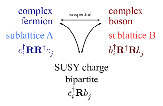
Figure 3: SUSY matching complex bosons and fermions - Schematic relation between complex bosons and fermions which can be connected by a SUSY charge defined on a bipartite lattice. In this case, both models are residing on its respective A and B sublattices.

We can also put our SUSY graph correspondence to work in a constructive manner. One natural way would be to start from a bipartite lattice, consider it to be a SUSY charge, and then identify two isospectral tight-binding models by decomposing it into its two sublattices. In the conceptual summary of our SUSY graph correspondence in Fig. 3 this corresponds to a start at the bottom and then working our way up. However, in practical settings one might be more interested in producing the supersymmetric partner for a given tight-binding model, e.g., by starting on the top left of Fig. 3 with a bosonic tight-binding model and asking whether it has a fermionic counterpart (or vice versa starting with a fermionic model and asking whether it has a bosonic counterpart). To construct such a SUSY partner, our graph square-root algorithm (which inverts the graph squaring of Fig. 2 as detailed in Appendix A) comes into play – it allows one to simultaneously construct both the supersymmetric lattice partners as well as the square-root bipartite lattice that decomposes into the two sublattices. If, for instance, one starts with the kagome lattice, one would readily identify the honeycomb lattice as its SUSY partner. Multiple other examples will follow in the next section making connections, e.g., between the square-octagon and squagome lattices (Fig. 7) or, in three spatial dimensions, the diamond and pyrochlore lattices (Fig. 16) or the hyperoctagon and hyperkagome lattices (Fig. 17).

All in all, the consequences of identifying supersymmetry with a graph correspondence seem quite substantial. The following parts of this manuscript are devoted to corroborate this by numerous examples in which the graph language greatly benefits the analysis and contextualization of various bosonic and fermionic lattice models.

II.4 Symmetry, Supersymmetry, and Topology

To complete our general discussion of SUSY-related bosonic and fermionic lattice models, we want to expand the underlying SUSY formalism to also reflect on Hamiltonian symmetries, band structure topology, and general classification of the connected models.

To start this discussion, it is important to revisit the SUSY charge operator in (3). It not only generates a pair of isospectral fermionic and bosonic Hamiltonians, it is itself associated with a third Hermitian operator

$$\mathcal{Q}_{\rm H}=\mathcal{Q}+\mathcal{Q}^{\dagger} =c^{\dagger}{\bf R}b+b^{\dagger}{\bf R}^{\dagger}c$$

$$\equiv\begin{pmatrix}c^{\dagger}&b^{\dagger}\end{pmatrix}\begin{pmatrix}&{\bf R}\\ {\bf R}^{\dagger}&\end{pmatrix}\begin{pmatrix}c\\ b\end{pmatrix}\,.$$ (12)

This operator is an arbitrary Hermitian quadratic form that anticommutes with fermion parity $e^{i\pi c^{\dagger}c}$. Its eigenspectrum is presented in the middle panel of the triptych-like figures, such as Fig. 1. For more details, see also the eigenstate mapping in Fig. 26 of the Appendix. Any deformation of the model parameters that preserves SUSY will map ${\cal Q}_{\rm H}$ to some other ${\cal Q}_{\rm H}^{\prime}$ and so we can define these SUSY preserving deformations as simply a deformation of ${\cal Q}_{\rm H}$ itself. The fermionic and bosonic Hamiltonians, on the other hand, are not generally deformable under SUSY preserving deformations for they must maintain nonnegative eigenvalues. Hence, $\mathcal{Q}_{\rm H}$ defines the topological classification of quadratic SUSY problems.

To classify ${\cal Q}_{\rm H}$, we will begin by identifying the symmetries of ${\cal H}_{F}$ and ${\cal H}_{B}$ that are important for the topological classification of fermionic problems. Then we will see how these symmetries map under SUSY so that knowing a symmetry of ${\cal H}_{F}$ aids in determining its form for ${\cal H}_{B}$ or vice versa. Finally, this understanding of symmetry will lead us to the classification of supersymmetric systems via $\mathcal{Q}_{\rm H}$.

It has become widely appreciated that one can use electronic band structure calculations to readily deduce topological properties [55]. Doing so rests on the fact that for fermionic systems, topological invariants are intimately connected to certain unitary and antiunitary symmetries [21] of the single particle Hamiltonian matrix.

In the case of a fermionic Hamiltonian, the action of the following set of symmetries is of pivotal importance: time-reversal symmetry ($\cal T$), particle-hole symmetry ($\cal P$), and chiral/sublattice symmetry ($\cal C={\cal T}\cdot{\cal P}$). $\cal T$ and $\cal P$ are anti-unitary symmetries that commute ($\cal T$) or anticommute ($\cal P$) with the single particle Hamiltonian matrix, while $\cal C$ is an anticommuting unitary symmetry. They square to the possible values of ${\cal T}^{2}=\pm 1,{\cal P}^{2}=\pm 1,{\cal C}^{2}=0,1$. Combining these symmetries leads to ten topologically distinct classes of Hamiltonians describing non-interacting fermionic systems [36].

Consider first the time-reversal symmetry for fermions and its mapping to bosons. Working in the Fourier space, the fermionic and bosonic eigenstates of ${\cal H}_{F}$ and ${\cal H}_{B}$, the Bloch wavefunctions $|u({\bf k})\rangle$ and $|v({\bf k})\rangle$, are related as

$$|u({\bf k})\rangle=\frac{{\bf R}({\bf k})}{\sqrt{\omega({\bf k})}}|v({\bf k})\rangle\quad{\rm and}\quad|v({\bf k})\rangle=\frac{{\bf R}^{\dagger}({\bf k})}{\sqrt{\omega({\bf k})}}|u({\bf k})\rangle\,.$$ (13)

This mapping is then associated with the operator

$$\tilde{\bf R}({\bf k})\equiv\frac{{\bf R}({\bf k})}{\sqrt{\omega({\bf k})}}\,,$$ (14)

which defines a norm-preserving map between the finite energy eigenstates of the concerned Hilbert spaces. But by construction this excludes the zero modes of the energy spectra $\omega({\bf k})$ of the two isospectral Hamiltonians ${\cal H}_{F}$ and ${\cal H}_{B}$. If the flat bands arise when $\nu>0$, i.e.,  when ${\bf R}$ is a rectangular matrix and annihilates the flat band states, then

$${\bf R}({\bf k})\leavevmode\nobreak\ |v_{\bf k}^{\rm(zero)}\rangle=0\,,$$ (15)

when $|v_{\bf k}^{\rm(zero)}\rangle$ is a state in the flat band manifold. Let us assume ${\cal P}_{\rm fb}$ is a projector onto this manifold. The full time-reversal operator spanning the entire bosonic Hilbert space (including the flat bands) then is related to the fermionic time reversal operator via (see Fig. 4)

$${\cal T}_{B}({\bf k}) =[1-{\cal P}_{\rm fb}({\bf k})]{\bf R}^{\dagger}(-{\bf k}){\cal T}_{F}({\bf k}){\bf R}({\bf k})[1-{\cal P}_{\rm fb}({\bf k})]$$

$$\leavevmode\nobreak\ \leavevmode\nobreak\ \leavevmode\nobreak\ \leavevmode\nobreak\ \leavevmode\nobreak\ \leavevmode\nobreak\ \leavevmode\nobreak\ \leavevmode\nobreak\ \leavevmode\nobreak\ \leavevmode\nobreak\ \leavevmode\nobreak\ \leavevmode\nobreak\ \leavevmode\nobreak\ \leavevmode\nobreak\ \leavevmode\nobreak\ \leavevmode\nobreak\ \leavevmode\nobreak\ \leavevmode\nobreak\ \leavevmode\nobreak\ \leavevmode\nobreak\ \leavevmode\nobreak\ \leavevmode\nobreak\ \leavevmode\nobreak\ \leavevmode\nobreak\ \leavevmode\nobreak\ \leavevmode\nobreak\ \leavevmode\nobreak\ \leavevmode\nobreak\ \leavevmode\nobreak\ \leavevmode\nobreak\ \leavevmode\nobreak\ +{\cal P}_{\rm fb}(-{\bf k})\Theta_{B}({\bf k}){\cal P}_{\rm fb}({\bf k})\,,$$ (16)

where $\Theta_{B}$ is a bosonic time-reversal operator that operates only within the flat band manifold (e.g.,  it can be $\Theta_{B}=U{\cal K}$ where $U$ is a unitary operator and ${\cal K}$ is the complex conjugation, both restricted to the flat band manifold). Therefore, the matrix form of ${\cal T}_{B}$ is block-diagonal

$${\cal T}_{B}=\left[\begin{array}[]{c|c}{\bf R}^{\dagger}{\cal T}_{F}{\bf R}&\\ \hline\cr&\Theta_{B}\end{array}\right],$$ (19)

where the upper block, corresponding to all finite energy states, is separated from the lower one, which consists of the zero modes (flat bands), by the projector ${\cal P}_{\rm fb}$. The time-reversal operator in (II.4) satisfies ${\cal T}_{B}(-{\bf k}){\cal T}_{B}({\bf k})=1$. If $\nu\leq 0$, the flat bands either do not arise or they arise on the fermionic side. Then the mapping is simpler

$${\cal T}_{B}({\bf k}) ={\bf R}^{\dagger}(-{\bf k}){\cal T}_{F}({\bf k}){\bf R}({\bf k})\,.$$ (20)

As a result, we generally expect the time reversal symmetry to map between the fermions and bosons.

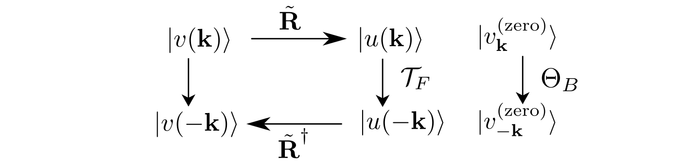
Figure 4: Time reversal symmetry under SUSY map. The category to define the bosonic time-reversal within the space of the finite-energy bosonic states $|v({\bf k})\rangle$ by combining the SUSY mapping to their fermionic partner states $|u({\bf k})\rangle$ and the time-reversal in the space of the fermionic states, ${\cal T}_{F}$. Another time-reversal operator $\Theta_{B}$ acts within the manifold of the zero modes $|v^{({\rm zero})}_{\bf k}\rangle$ separated by the projector ${\cal P}_{\rm fb}$. Together, they define the full bosonic time-reversal ${\cal T}_{B}$ in (II.4) .

Such a mapping cannot be constructed for the bosonic particle-hole operator ${\cal P}_{B}$ when $\nu>0$. This is because, when restricted to the flat band manifold which maps onto itself under particle-hole conjugation, it reduces to the time-reversal operator ${\cal T}_{B}$ only. As a result, such identification in this case also fails to apply for the bosonic chiral symmetry operator ${\cal C}_{B}={\cal T}_{B}\cdot{\cal P}_{B}$ which is trivial in the presence of the flat bands. These situations are easily established when the SUSY for $\nu\neq 0$ identifies a bipartite fermionic system (e.g., on the honeycomb lattice) with a non-bipartite bosonic system (e.g., on the kagome lattice). The absence of a mapping between the fermions and bosons for ${\cal P}$ and ${\cal C}$ is then directly associated with the loss of the bipartite property of the lattice.

With both the symmetries and the Hermitian operator $\mathcal{Q}_{\rm H}$ identified, we are now in a position to classify our SUSY models. First, consider the case with no symmetry, just supersymmetry. We see that fermion parity $e^{i\pi c^{\dagger}c}$ is an anticommuting unitary operator which acts at the single particle level as the anticommuting unitary matrix

$${\cal C}_{\rm SUSY}=\begin{pmatrix}{\bf I}&\\ &-{\bf I}\end{pmatrix}.$$ (21)

So all SUSY problems are chiral. Then adding the additional symmetries $\mathcal{T}$, $\mathcal{P}$ and $\mathcal{C}$ that act on both fermions and bosons as discussed above we see that we cannot additionally add a $\mathcal{C}$ since a chiral symmetry is already present. And, if we add $\mathcal{T}$, we automatically obtain a $\mathcal{P}$ for $\mathcal{C}=\mathcal{T}\cdot\mathcal{P}$. As a result, we avoid the difficulty with deriving ${\cal P}_{B}$ from ${\cal P}_{F}$ pointed out above. The bipartite-ness of $\mathcal{Q}_{\rm H}$ naturally enables a $\mathcal{P}$ symmetry. Hence, in classifying the SUSY problems, either we do not have $\cal{T}$ and $\cal{P}$ or we have them both with one derivable from the other.

With that, we arrive at a five-fold way classification of SUSY models characterized by the absence of $\mathcal{T}_{\rm SUSY}$/$\mathcal{P}_{\rm SUSY}$ (class AIII) and the four classes with $\mathcal{T}_{\rm SUSY}$, $\mathcal{P}_{\rm SUSY}$ having $\mathcal{T}_{\rm SUSY}^{2}=\pm 1$, $\mathcal{P}_{\rm SUSY}^{2}=\pm 1$ (classes BDI, CI, CII, DIII). Previously, two of us classified the related problem of rigidity matrices [43, 41] and found a three-fold classification (classes AIII, BDI, and CII). So by classifying ${\cal Q}_{\rm H}$, we have now found two previously unknown classes of SUSY Hamiltonians.

To construct a classification table, we need to identify the topology of the classifying space of $\mathcal{Q}_{\rm H}$ in each of the five symmetry classes. Following the classification of rigidity matrices [43], we can arrive at this by carrying out a singular value decomposition of a generic rectangular ${\bf R}$ matrix of dimension $M\times N$ as ${\bf R}={\bf U}{\bm{\Sigma}}{\bf V}^{\dagger}$ ($\bf U$ and $\bf V$ are unitary matrices of dimension $M\times M$ and $N\times N$ respectively) and smoothly flatten the singular values ${\bm{\Sigma}}\to{\bf I}_{M\times N}$. The resulting flattened matrix then lives in a potentially non-trivial topological space defined by the gapping condition that no singular values vanish. The effect of this transformation on $\mathcal{Q}_{\rm H}$ is to place it in the form

$$\mathcal{Q}_{\rm H}\to\begin{pmatrix}{\bf U}&\\ &{\bf V}\end{pmatrix}\begin{pmatrix}&{\bf I}_{M\times N}\\ {\bf I}_{N\times M}&\end{pmatrix}\begin{pmatrix}{\bf U}^{\dagger}&\\ &{\bf V}^{\dagger}\end{pmatrix}.$$ (22)

Inserting $e^{i(\pi/4)\bm{\sigma}_{y}}$, we can rotate this expression into an eigenvalue decomposition

$$\mathcal{Q}_{\rm H}\to{\bf P}\begin{pmatrix}{\bf I}_{M\times M}&&\\ &-{\bf I}_{M\times M}&\\ &&{\bf 0}_{(N-M)\times(N-M)}\end{pmatrix}{\bf P}^{\dagger},$$ (23)

with

$${\bf P}=\begin{pmatrix}{\bf U}&\\ &{\bf V}\end{pmatrix}e^{i(\pi/4)\bm{\sigma}_{y}},$$ (24)

where, without loss of generality, we have considered $M<N$. For the case $\nu=0$, where ${\bf R}$ is a square matrix with $M=N$, the singular value gapping condition is identical to the eigenvalue gapping condition for all five classes AIII, BDI, CI, CII, and DIII. For $\nu\neq 0$, however, we arrive at a space of Hermitian matrices where some eigenvalues are forced to vanish by SUSY. These eigenvalues appear as protected flat bands in SUSY band structure calculations. The gapping condition now corresponds to a pair of (positive and negative) eigenvalues vanishing to create additional zero eigenvalues. An example in band structures is a nexus point [56, 57, 58, 59]: a point where multiple energy bands merge in a three- or higher-fold degenerate fashion (including, in particular, a possible combination with flat bands, which will be the case for most of our examples). Hence, by flattening the eigenvalues of $\mathcal{Q}_{\rm H}$, we map it onto certain spaces of matrices which can have non-trivial topology.

BDI				Figures with examples
$\quad\nu\quad$	$\quad\pi_{1}\quad$	$\quad\pi_{2}\quad$	$\quad\pi_{3}\quad$	$\quad\pi_{1}\quad$	$\quad\pi_{2}\quad$	$\quad\pi_{3}\quad$
1	$\mathbb{Z}_{2}$	0	$\mathbb{Z}$	1,24	–	–
2	0	$\mathbb{Z}$	$\mathbb{Z}$	–	8,16,17	(8,16,17)
3	0	0	$\mathbb{Z}$	–	–	–
4	0	0	0	–	–	–

Table 1: Topological classification of SUSY Hamiltonians with finite Witten index. The table (on the left) indicates topological invariants ($\mathbb{Z}_{2}$, $\mathbb{Z}$) as a function of Witten index $\nu$. It is organized not by the spatial dimension used in the ten-fold way table [37, 38, 39, 40] but by homotopy groups $\pi_{n}$. Mathematically, the latter correspond to maps from $n$-dimensional sphere ${\cal S}_{n}$ to the flattened SUSY charge in (22). In physical terms, $\pi_{1}$ is also known as the Berry phase and $\pi_{2}$ as the Chern number, which we here associate with features (such as nexus points) of the zero-energy band of the SUSY charge band structure (depicted in the middle panel of the triptych-like figures of Section III). Shown are the results for the symmetry class BDI [43]; four more symmetry classes are discussed in Appendix B leading to a five-fold way classification scheme, fully tabulated in Table 4 of the Appendix. On the right, we tabulate example systems (illustrated in the respectively linked figures) with non-trivial topological index, including the SUSY charge on the following lattice geometries: honeycomb-X (Fig. 1), square-X/Lieb lattice (Fig. 24), hyperhoneycomb-X (Fig. 8), diamond-X (Fig. 16), and hyperoctagon-X (Fig. 17). The non-trivial homotopy groups associated with certain features in their respective band structure are illustrated in Fig. 23 of the Appendix.

The final steps are to identify the topology of the classifying spaces and to compute topological invariants to identify protected zero modes. We carry these steps out in Appendix B where we present complete example calculations along with tables of homotopy groups associated with each class, dimension, and Witten index $\nu$. It turns out, all of the examples in the next section, Section III, are in the BDI symmetry class. To highlight their potential topological zero modes, we therefore present in Table 1 the BDI table produced in Appendix B and the figures that present the associated examples.

In summary, the SUSY band structures that fit into the formalism of this paper fall into the five-fold classification of chiral Hamiltonians. For the case $\nu=0$, we can resort to the ten-fold way to classify $\mathcal{Q}_{\rm H}$ while for $\nu\neq 0$ we can rely on Ref. [43] for classes AIII (unitary), BDI (orthogonal) and CII (symplectic). Building on these references, Appendix B presents the five tables classifying the SUSY band structures.

III Frustrated magnets

In putting our SUSY correspondence to work, let us turn to the phenomenology of frustrated magnets as one realm to highlight the conceptual insights one might quickly derive in connecting them to SUSY-related free-fermion systems. One such insight relates to the Maxwell counting for geometrically frustrated magnets, which we will discuss in the language of our SUSY correspondence in Section III.1. Another insight is that SUSY allows for a classification of extensive ground-state manifolds in classical spin models, which we will subsequently turn to in subsection III.2. Our SUSY correspondence can also be employed to predict magnon dispersions for certain frustrated magnets in large magnetic fields, which we will discuss in subsection III.3, and parton dispersions for certain quantum spin liquids, in subsection III.4.

III.1 Maxwell counting for geometrically frustrated magnets

The first case study of our SUSY formalism in the context of frustrated magnetism concerns the special class of geometrically frustrated magnets that can satisfy a total spin constraint on each simplex (or fully connected plaquette in the parlance of the current manuscript) of the lattice [33, 34]. Common examples include kagome and pyrochlore Heisenberg antiferromagnets where these simplices correspond to triangles and tetrahedra, respectively. But less common examples are also possible such as distorted kagome antiferromagnets [35] and even the square lattice Neél antiferromagnet since a two-site bond can also be viewed as a simplex [22] or a fully connected plaquette, as indicated in Fig. 2. To see the presence of these spin constraints, we need to write the spin model Hamiltonian as a perfect square

$$H=\sum_{\langle ij\rangle}J_{ij}{\bf S}_{i}\cdot{\bf S_{j}}+\text{const.}=\frac{1}{2}\sum_{\Delta}\bigg{[}\sum_{i\in\Delta}a_{i}{\bf S}_{i}\bigg{]}^{2}\,,$$ (25)

where $\Delta$ denotes the simplex of the lattice, we keep spin rotation invariance for simplicity, and generalize the total spin constraint to include the $a_{i}$ factors. Note the similarity of this perfect square formulation to a balls-and-springs model with potential energy $\frac{1}{2}ke_{m}^{2}$, $e_{m}$ the extension of spring $m$, such as those discussed below in section IV. This special form of the Hamiltonian enables a SUSY correspondence [22], which we will cast in our general framework in the following.

We can identify both a quantum and a classical SUSY model from the perfect square Hamiltonian (25). In the quantum case, the individual terms of the Hamiltonian do not generally commute with one another and therefore cannot be simultaneously satisfied in the ground state. In the classical case, however, each term in the Hamiltonian can be simultaneously satisfied, thereby defining a set of Maxwell constraints. Let us, in the following, first visit the quantum case and the behavior of magnon excitations of an ordered state and then turn to the classical case to illustrate the role of SUSY and the relation between the Witten index and Maxwell counting in geometrically frustrated magnets.

Quantum antiferromagnets

In the quantum case, we can define a supersymmetric charge from the total spin on a simplex by associating a fermion with each component of this spin in the large-$S$ limit [22]. For simplicity, we will study a pure XY quantum model, similar to those studied for their connections to gauge theories [60] or deconfined quantum criticality [61]. For such models, we can construct the SUSY charge

$${\cal Q}=\sqrt{\frac{J}{2}}c^{\dagger}_{\Delta}S^{-}_{\Delta}\,,$$ (26)

where $S^{-}_{\Delta}=\sum_{j\in\Delta}(S_{jx}+iS_{jy})$. It has a U(1) symmetry in which spin rotations around the $z$-axis, $S_{\Delta}^{-}\to e^{i\theta}S_{\Delta}^{-}$, are absorbed into a phase change of the fermions $c_{\Delta}^{\dagger}\to e^{-i\theta}c_{\Delta}^{\dagger}$, and leads to the SUSY Hamiltonian $\frac{1}{2}\{{\cal Q},{\cal Q}^{\dagger}\}$

$$H_{\rm SUSY}\!=\!\frac{J}{2}\!\sum_{\Delta}\!\left({\bf S}_{\Delta}^{2}\!+\!(1\!-\!2c^{\dagger}_{\Delta}c_{\Delta})S^{z}_{\Delta}\right)-J\!\!\!\sum_{\langle\Delta\Delta^{\prime}\rangle}c^{\dagger}_{\Delta}S^{z}_{\Delta\Delta^{\prime}}c_{\Delta^{\prime}}\,,$$ (27)

where the first term is the perfect square Hamiltonian of (25) with $a_{i}=1$, ${\bf S}_{\Delta}$ the total $xy$-spin of simplex $\Delta$, $S^{z}_{\Delta}$ the total z-component of simplex $\Delta$, and $S^{z}_{\Delta\Delta^{\prime}}$ the $z$-component of the spin on the site shared by neighboring simplices $\Delta$ and $\Delta^{\prime}$. In this way, we arrive at an interacting SUSY problem where fermions and bosons know about each other’s existence. Since the spin model Hamiltonian of (25) does not involve spins interacting with fermions, this new model is not directly related to the original one. But we will see that in the large-$S$ limit, the fermions and bosons decouple and, at the quadratic level, the magnons of a geometrically frustrated magnet of the kind we are discussing here will have a fermionic SUSY partner.

As the avid reader might have already noticed, the formulation in terms of an effective total spin on a simplex bears some similarity to the lattice construction algorithm of Fig. 2 (and outlined in Appendix A) as it groups edges of the lattice in terms of fully connected plaquettes. Building a SUSY charge by combining such a fully connected plaquette of the original lattice with a new particle in its center, a fermion in this case, is graphically equivalent to introducing a new vertex in the center of a clique and connecting it with all existing vertices of this clique. For instance, for the case of an XY model on the kagome lattice, the $c$ and $c^{\dagger}$ are placed on the honeycomb lattice, formed by the center of the triangles of the kagome lattice – or, in the parlance of this manuscript, the SUSY partner of the kagome lattice.

To decouple the fermions and bosons, in a subsequent step, we expand around a ground state of the magnetic system. We do so by expressing the on-site spin operators $S^{\pm}_{j}=S^{x}_{j}{\pm}iS^{y}_{j}$ and $S^{z}_{j}$ in terms of Holstein-Primakoff [62] bosonic (magnon) annihilation and creation operators $b_{j}$ and $b_{j}^{\dagger}$ as

$$S^{+}_{j}=\sqrt{2S-n_{j}}\leavevmode\nobreak\ b_{j}\leavevmode\nobreak\ ;\leavevmode\nobreak\ S^{-}_{j}=b^{\dagger}_{j}\sqrt{2S-n_{j}}\leavevmode\nobreak\ ;\leavevmode\nobreak\ S^{z}_{j}=S-n_{j},$$ (28)

where $n_{j}=b_{j}^{\dagger}b_{j}^{\phantom{\dagger}}$ measures the on-site magnon occupancy. In general we do so differently on each site, choosing the $z$-direction to point along the local magnetic ordering vector.

We can attempt to expand the SUSY charge to order $\sqrt{S}$ in a large-$S$ expansion. Doing so, we obtain a SUSY charge similar in form to (3)

$${\cal Q}=c^{\dagger}{\bf R}_{1}b+c^{\dagger}{\bf R}_{2}b^{\dagger}\,,$$ (29)

but here there are two matrices ${\bf R}_{1}$ and ${\bf R}_{2}$ unlike in (3). We can also wonder if the approximation preserves the SUSY algebra that demands ${\cal Q}^{2}=0$. We find

$${\cal Q}^{2}=c^{\dagger}{\bf R}_{1}{\bf R}_{2}^{T}c^{\dagger}\,.$$ (30)

This would be a pairing term in the fermion Hamiltonian. For all the cases we discuss below, we find fermion pairing vanishes and ${\cal Q}^{2}=0$, the ${\cal N}=2$ SUSY algebra is preserved by the large-$S$ approximation.

Proceeding to derive the SUSY Hamiltonian, via $H_{\rm SUSY}=\frac{1}{2}\{Q,Q^{\dagger}\}$, yields

$$H_{\rm SUSY}=\frac{1}{2}c^{\dagger}({\bf R}_{1}{\bf R}_{1}^{\dagger}-{\bf R}_{2}{\bf R}_{2}^{\dagger})c\\ +\frac{1}{2}b^{\dagger}({\bf R}_{1}^{\dagger}{\bf R}_{1}+{\bf R}_{2}^{T}{\bf R}_{2}^{*})b+\left(b\,{\bf R}_{2}^{\dagger}{\bf R}_{1}b+{\rm h.c.}\right)\,.$$ (31)

Thus, expanding around a ground state of the XY model (spontaneously) violates the U(1) symmetry of magnons but not of the fermions – the superfluid of magnons are partnered with metallic fermions.

Now, in this XY model, there are many large-$S$ ground states, each with their own magnon band structure. These ground states define the frustration: the spins struggle to choose the best from among all the ground state options. One way to understand this frustration is to take a walk along a path in the ground state manifold and, stopping at points along the walk, study the magnon band structure. Let us do so in a kagome lattice example.

One “ferrimagnetic” walk in the kagome lattice XY model defined above, is to start from the antiferromagnetic “$q=0$ state” defined by three spin ordering vectors ${\bf A}$, ${\bf B}$, ${\bf C}$ lying in the $xy$-plane with ${\bf A}+{\bf B}+{\bf C}=0$; placing one on each of the three sites in the unit cell. Then add a $z$-component uniformly to all three ordering vectors, capturing this change by the polar angle $\theta$ that is $\pi/2$ in the $q=0$ state and zero in the fully tilted simple ferromagnetic state. This walk then takes us from a classic antiferromagnetic state to the fully polarized ferromagnetic state.

In Fig. 5, we present the evolution of the magnon band structure and their SUSY partner along the above walk. It shows at all points except $\theta=\pi/2$, that the ferrimagnetic states reproduce Fig. 1 – the magnons have a flat band with a quadratic band touching at the $\Gamma$-point (with a non-trivial $\pi_{1}$-topology) and a semimetal as a SUSY partner. These states preserves the XY spin rotational symmetry of the spins and the $U(1)$ symmetry of a metal. But the bandwidth depends on the point along the walk and vanishes as the purely antiferromagnetic point $\theta\to\pi/2$ is reached. At this special point, flat bands emerge in both the magnon and partner fermion models.

We can take a second walk in the infinite dimensional space of ground states of the large-$S$ spin model, this time following a purely antiferromagnetic trajectory. Here we begin with the $q=0$ state and rotate it out of the $xy$-plane, keeping $S_{\Delta}^{z}=0$. This can be achieved by rotating about the ${\bf B}$ direction by an amount $\alpha$, a rotation that lifts the ${\bf A}$ spins above the plane and ${\bf C}$ spins below the plane. Surprisingly, this rotation has no effect on the band structure: all of these antiferromagntic states have a vanishing magnon bandwidth.

These results suggest thermal order-by-disorder would be different from quantum order-by-disorder. Thermal order-by-disorder is entropic selection of ground states that results from warming up the system from its $T=0$ ground state. For the kagome XY model, we would expect a much larger entropy for the antiferromagnetic states than the ferromagnetic states and so an antiferromagnetic state would be selected at large-$S$ but finite $T$. On the other hand, the pure ferromagnetic state at $\theta=0$ is an eigenstate of the full interacting Hamiltonian. This state has the least quantum fluctuations and so is the most stable ground state. It should be selected at finite $S$, $T\to 0$. So the two limits do not commute and we expect the ordering tendencies will be different between thermal and quantum fluctuations, much like the $q=0$ is selected by quantum fluctuations while the higher entropy $\sqrt{3}\times\sqrt{3}$ state (not discussed here) is selected by thermal fluctuations in the XXZ kagome antiferromagnet [63].

Before concluding, we must comment on the full interacting theory. The Hamiltonian of (27), preserves magnon number and has many known eigenstates [64]. Hence, the ferromagnetic (zero-magnon) ground state, the one-magnon states, the two-magnon states, etc. are all mapped to themselves by $H_{\rm SUSY}$ and captured by small matrices. Specifically, we find the “all down” spin state with zero fermions per site and the “all up” spin state with one fermion per site are exactly at zero energy. In addition to these two zero-magnon states, we find the one-magnon states, produced by the linear combinations of the all down state raised by one unit of angular momentum, $S_{i}^{+}|-S,-S,\ldots\rangle$, or lowing the all up state by one unit of angular momenum, $S_{i}^{-}|S,S,\ldots\rangle$, have exactly the band structure of the bosonic dispersions plotted in Fig. 5 with the flat band at zero energy and a bandwidth of $6JS$. Hence, there are an infinite number of zero modes among the one-magnon states. Similarly, we find two zero energy states among the one-fermion states, the states corresponding all-down spins with one fermion occupying the ${\bf k}=0$ state and the all up state with one hole occupying the ${\bf k}=0$ hole-state. There are clearly more zero energy states than these. In total, we find an infinite number of exact ferromagnetic eigenstates in the SUSY model of (27). We have not identified any antiferromagnetic eigenstates and do not expect to do so. We conjecture these all are lifted to finite energy by quantum fluctuations and are only at zero energy in the classical $S\to\infty$ limit. Hence, we still expect ferromagnetism to be selected by quantum fluctuations.

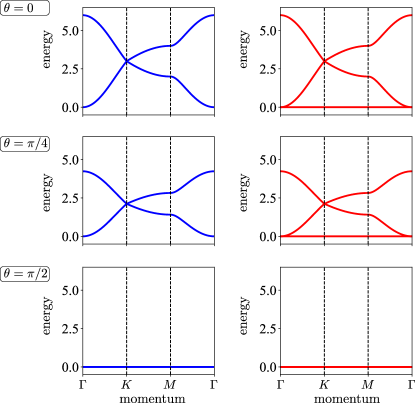
Figure 5: Kagome lattice magnons (right) and their SUSY partner (left). Spectra are shown along a “ferrimagnetic” path in the XY model ground state manifold: at the $z$-polarized ferromagnetic point $\theta=0$ (top), at $\theta=\pi/4$ in the ferrimagnetic region (middle), at the antiferromagnetic $q=0$ point $\theta=\pi/2$ (bottom). These band structures show how ferromagnetic magnons have a quadratic band-touching semimetal as a SUSY partner. Similar to the band structure in Fig. 1, we note that the Witten index is $\nu=1$ for all three panels with the quadratic band touching (in the two upper panels) exhibiting a non-trivial $\pi_{1}$-topology.

Classical Maxwell Counting

In the previous discussion, we computed the band structure of a large-$S$ kagome XY model and found a flat band of magnons partnered with metallic fermions. Let us turn our attention to the existence of this flat band, for in these models, it is the fundamental cause of their frustration effects.

The SUSY charge of (26), introduces one complex fermion on each simplex and, at the classical level, two total spin constraints imposed on the ground state by the ${\bf S}_{\Delta}^{2}$-term. Expressing the complex fermion as two real fermions $c^{\dagger}_{\Delta}=\gamma_{\Delta x}-i\gamma_{\Delta y}$ suggests that we have fermionized the constraints: $\gamma_{\Delta x}$ corresponds to the $S_{\Delta x}=0$ constraint and $\gamma_{\Delta y}$ to the $S_{\Delta y}=0$ constraint. Similarly, one complex boson $b_{i}$ suggests that we have two real “degrees-of-freedom” per site. Hence, from a real-fermion, real-boson perspective, the single particle Witten index, that counts the difference between the number of bosons and fermions, corresponds in the classical limit to Maxwell counting: The number of “degrees of freedom” minus the number of constraints is twice the number of complex boson operators $b_{i}$ minus twice the number of complex fermion operators $c_{\Delta}$. In this way, we can exactly reproduce Moessner and Chalker’s Maxwell counting [33, 34] in a supersymmetric theory.

For the specific case of the kagome XY model discussed above, the Maxwell counting works out to four constraints per unit cell (which has two triangles) and 6 real degrees of freedom (three spins). Hence, Maxwell counting tells us there is a minimum of $\nu=6-4=2$ real degrees of freedom, i.e. one complex degree of freedom, per unit cell. This therefore demands the existence of one flat band in the magnon-number preserving band structure as presented in Fig. 5.

Maxwell counting involves more than identifying flat bands, it also enables topology through topological mechanics [7]. In this vein, topological properties of magnons in distorted kagome antiferromagnets were studied in Ref. 35 by placing them in the form of (25). This study found two classes of problems associated with a triangulated surface in spin space called spin origami [65, 66, 67]. Flattenable spin origami with a flat band of zero energy magnons, and non-flattenable spin origami with Fermi-surface like degeneracy of magnons. These results are due to SUSY [22], but SUSY was not employed directly in obtaining them. Nevertheless, the topological property of spin waves discussed in this paper is precisely that expected by the supersymmetry encoded in (26) upgraded to Heisenberg spins, an upgrade that is possible [22] with the real formalism discussed in Section IV.

In summary, we have demonstrated the use of SUSY and our lattice construction to find highly frustrated magnets, materials whose magnons exhibit a flat band at different points on their large-$S$ ground state manifold. Using an XY model as an example, a model with a global $U(1)$ symmetry, and following Ref. 22, we wrote down a SUSY charge assigning a fermion creation operator to the $xy$-plane component of the total spin constraint on a simplex. This approach reproduced the Moessner-Chalker-Maxwell counting [33, 34] identifying highly frustrated magnets as underconstrained systems, recognizing that such counting formally is associated with a SUSY system. This formal connection revealed a hidden U(1) symmetry of the magnons in the example studied – their fermionic partner is a semimetal instead of a superfluid. But in addition, our identification of such systems is broader than Moessner and Chalker, capturing lattices that go beyond corner sharing simplices.

III.2 Ground-state manifolds

As a second case study for our SUSY framework we will exclusively turn to classical spin models, which are often considered as first steps in the search for unconventional forms of magnetism. Conceptual advances such as the discussion of residual entropies [68, 69] as a defining signature of frustration [70, 71] or the identification of cooperative paramagnetism [72], emergent Coulomb phases [73], or order-by-disorder phenomena [74] have been formulated in the context of such classical models alongside the establishment of classical spin liquids [75] and spin ice [76, 77]. Many of these phenomena are evolving around extensive ground-state manifolds of geometrically frustrated Heisenberg antiferromagnets.

Here we will apply our SUSY framework to accomplish two conceptual goals in this context. First, we will explicate how the SUSY lattice correspondence leads one to quickly identify lattice geometries for which Heisenberg antiferromagnets are likely to exhibit extensive ground-state manifolds. One prime example is the (classical) kagome antiferromagnet which we connected to the honeycomb-kagome case study in our introduction (Fig. 1). We will also see many other instances in two and three spatial dimensions in this section, which are all exemplified by similar triptych-like figures, such as Fig. 16 below which makes the case for the pyrochlore antiferromagnet. Second, we will use our framework to recast a spin-fermion correspondence in terms of our SUSY framework, which had been formulated by some of us [78] to provide a link between the spin spiral ground-state manifolds of frustrated spin models and Fermi surfaces of electronic tight-binding models.

Luttinger-Tisza method

The starting point for our discussion is a classical Heisenberg antiferromagnet whose Hamiltonian we write as

$$\mathcal{H}_{\text{Heisenberg}}=\sum_{ij}M_{ij}\,{\bf S}_{i}\cdot{\bf S}_{j}\,,$$ (32)

where the three-component vectors ${\bf S}=(S^{x},S^{y},S^{z})$ denote $O(3)$ spins and $M_{ij}$ describes the (antiferromagnetic) coupling between two spins at real space coordinates $i$ and $j$. For a given lattice structure, the individual $M_{ij}$’s reflect the connectivity of this geometry and constitute the entries of a (weighted) adjacency matrix $\bf M$.

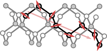
Figure 6: Coplanar spin spirals. Schematic drawing of a coplanar spin spiral on the diamond lattice. Heisenberg spins on every site enclose a fixed angle when traversing through the lattice along the spiral wavevector (as indicated by the faint background arrow). Such phases are relevant as ground states of many classical frustrated antiferromagnets.

We are interested in the ground states minimizing the energy of this Hamiltonian, which, under certain circumstances, one can identify analytically using the Luttinger Tisza (LT) method [79, 80]. This method is based around the observation that any ground state minimizing (32) is also a ground state of the unconstrained problem where $|{\bf S}_{i}|\neq 1$. Hence, solving the unconstrained problem first using linear algebra can enable the solution of the constrained problem. For certain lattices, this attempt at a solution always succeeds and leads to coplanar spin spirals (see Fig. 6) with the same unit cell as the underlying lattice. Not all classical spin ground states can be characterized in this way, but Heisenberg models have a tendency to do so [81].

Specifically, the LT approach proceeds by Fourier transforming the interaction matrix of (32) to its momentum space representation $\mathbf{M}({\bf k})$ and diagonalizing it for a given momentum $\bf k$ – a step that is strongly reminiscent of tight-binding calculations and which we will build upon in the following. Before doing so, let us point out a key distinction here in that one still has to reconstruct the real-space coplanar spin spiral once one has identified the momentum ${\bf k}$ of the minimal eigenvalue. The wavevector of this spin spiral is simply given by ${\bf k}$ and phases of individual spins within the real-space basis can be read off the eigenstate itself as long as the equal-length hard-spin constraint is fulfilled – a constraint which we have effectively relaxed when simply diagonalizing $\mathbf{M}({\bf k})$. For Bravais lattices, however, this constraint must be generically fulfilled [82], while for non-Bravais lattices this must not be the case and, by enforcing the constraint, one might end up selecting a subset of states found by the minimization.

Extensive degeneracies and flat bands

One approach of equating the LT approach to a band structure calculation is to identify, on the level of matrix equivalences, the spin interaction matrix with the (bosonic) right-hand side of Fig. 3. We do this using the algorithm presented in Appendix A, which allows us to express ${\bf M}={\bf R^{\dagger}R}$. In doing so, the lattice correspondence of our SUSY framework identifies our LT calculation on some lattice (such as the kagome) with a free-fermion calculation on some other lattice (such as the honeycomb) as isospectral up to zero modes. But it is exactly the possible formation of such zero-energy flat bands that we are after when asking whether the Heisenberg antiferromagnet on some given lattice possibly has an extensive ground-state manifold. The kagome-honeycomb SUSY identification alluded to above, is precisely of this sort and lets us conclude that the kagome antiferromagnet has an extensive ground-state degeneracy.

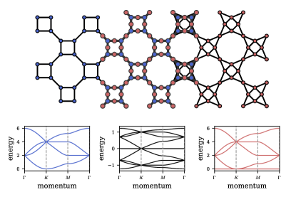
Figure 7: SUSY correspondence of square-octagon and squagome lattices. Complex fermions (blue, left) on the square-octagon lattice are supersymmetrically linked to complex bosons (red, right) on the squagome lattice. The mapping can be established with a SUSY charge which can be interpreted as the adjacency matrix of a square-octagon-X lattice (center plot), i.e., a square-octagon lattice with additional sites on every bond. For the topological classification according to Table 1, we find, noting that the Witten index here is $\nu=2$, that the nexus point in the SUSY charge spectrum has a trivial topological invariant of $\pi_{2}=0$, see also the illustration in Fig. 23 of the Appendix.

This idea can be readily generalized to other lattice geometries. In two spatial dimensions, one might consider the squagome antiferromagnet (Fig. 7), which has recently drawn some attention for the possible experimental realization of a spin liquid state in KCu₆AlBiO₄(SO₄)₅Cl [83]. The squagome is SUSY-related via our lattice correspondence to the square-octagon lattice (hence its name), whose smaller unit cell has two sites less than the one of the squagome lattice; this gives rise to a Witten index of $\nu=2$ and two flat bands in the squagome spectrum pointing to an extensive ground-state degeneracy and the formation of a classical spin liquid ground state [84, 85] similar to the case of the kagome antiferromagnet.

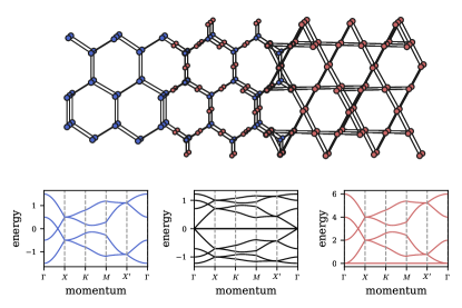
Figure 8: The hyperhoneycomb lattice and its SUSY partner. The hyperhoneycomb (10,3)b lattice (left) is connected to a three-dimensional lattice of corner-sharing triangles which bears some similarity to the two-dimensional kagome lattice but which should be distinguished from the hyperkagome lattice of Fig. 17. For the topological classification according to Table 1, we find, noting that the Witten index here is $\nu=2$, that the nexus point in the SUSY charge spectrum has a non-trivial topological invariant of $\pi_{2}=+1$, see also the illustration in Fig. 23 of the Appendix.

In three spatial dimensions, a well-known spin model with an extensive ground-state manifold is the classical pyrochlore antiferromagnet (Fig. 17 below), which can also be captured by our SUSY-framework as the pyrochlore lattice is SUSY-connected via our lattice correspondence to the diamond lattice – the two additional sites in the pyrochlore unit cell (with regard to the one of the diamond lattice) indicate a Witten index of $\nu=2$ and the formation of two flat bands in the pyrochlore spectrum, the harbingers of an extensive ground-state degeneracy, spin liquid, and spin ice physics [33, 34].

As a final example, we can also construct a possibly interesting three-dimensional lattice geometry, which has not received much attention so far, by applying our SUSY graph correspondence to the tricoordinated hyperhoneycomb lattice (Fig. 8), which has been investigated in the context of the Kitaev material $\beta$-Li₂IrO₃ [86]. To do so, we employ our lattice construction (Fig. 2) to arrive at a three-dimensional structure of corner-sharing triangles, depicted on the right-hand side of Fig. 8. The latter might have deserved to be named hyperkagome, which however has been taken by the distinct lattice geometry of Fig. 17 that is SUSY-related to the hyperoctagon lattice (both of which share a screw symmetry that is absent in the lattice geometries at hand). The point here is that our SUSY correspondence allows us to readily infer that the Heisenberg antiferromagnet on this lattice of corner-sharing triangles will exhibit an extensive ground-state degeneracy (i.e., a flat band in its LT spectrum) and as such likely a spin liquid ground state. This observation is expected to generally hold for the SUSY-partners of the entire family of tricoordinated lattices in three spatial dimensions [87, 88, 89].

Spin spirals and Fermi surfaces

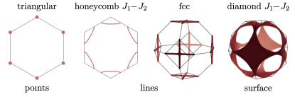
Figure 9: Spin spiral manifolds. Shown are the ground-state manifolds of coplanar spin spirals, exemplified by their respective $\bf k$ wavevectors in momentum space. Heisenberg antiferromagnets on different lattice geometries exhibit manifolds of varying dimensionality – points for the triangular lattice, lines for the fcc lattice and $J_{1}-J_{2}$ honeycomb model, as well as entire surfaces for the $J_{1}-J_{2}$ diamond lattice.

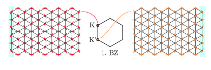
Figure 10: 120 degree order in the classical Heisenberg antiferromagnet on the triangular lattice. The two possible ordering patterns (left and right) correspond to wavevectors $\bf K$ and $\bf K^{\prime}$ at the corners of the Brillouin zone (BZ).

Another approach of relating the LT approach for classical Heisenberg models to electronic band structure calculations is motivated by the observation that, for many geometrically frustrated antiferromagnets, the manifold of coplanar spin spiral ground states resembles a Fermi surface [78]. Probably the most striking example is the $J_{1}-J_{2}$ Heisenberg antiferromagnet on the diamond lattice [90], for which the manifold of spin spiral states evolves as a function of $J_{2}/J_{1}$ from a spherical geometry (for small $J_{2}/J_{1}$) to an open topology as depicted in Fig. 9 (for intermediate $J_{2}/J_{1}$), and collapses into one-dimensional lines in the limit of $J_{2}/J_{1}\to\infty$, which corresponds to two decoupled face-centered cubic (fcc) lattices, also illustrated in Fig. 9. While the above cases relate to classical spin liquid ground states and systems with (sub)extensive ground state manifolds, one can also make such a connection between coplanar spin spirals and nodal electronic states for ordered classical states. Take, for instance, the triangular lattice Heisenberg antiferromagnet with its well-known 120 degree ordered ground states (Fig. 10); in momentum space the two possible ordering patterns of this 120 degree order correspond to momentum vectors $\bf K$ and $\bf K^{\prime}$ at the corners of the Brillouin zone – the well-known location of the Dirac cones of the honeycomb tight-binding model for free fermions. That one can indeed relate these two situations in a one-to-one SUSY correspondence in a similar way as one can connect the line-like or surface-like spin spiral manifolds above to the nodal lines or Fermi surfaces of SUSY-related electronic models will be the second SUSY correspondence for LT calculations that we will discuss here.

The conceptual difference to the first scenario above is that we are now aiming to connect a ground-state property of the classical spin model, captured by the minimal energies in the LT spectrum, to what is typically a mid-spectrum feature – the Fermi surface of an electronic tight-binding model. But in the language of our SUSY correspondences this immediately brings to mind that we might want to connect to the spectrum of the SUSY charge and the tight-binding spectrum of its lattice model. Let us exemplify this for the 120 degree order of the triangular lattice antiferromagnet. Our SUSY lattice correspondence (Fig. 2) connects the triangular lattice via a square-root to the honeycomb lattice whose two triangular sublattices are SUSY partners as established before and illustrated in our triptych-like form in Fig. 11. But when drawing our attention to the SUSY charge itself and its tight-binding spectrum in the middle panel of Fig. 11, we indeed find the correspondence that we have been looking for – the minima of the LT spectrum [left and right in Fig. 11 at $\bf K$ (and $\bf K^{\prime}$, not shown)] get mapped to the Dirac points in the middle of the well-known electronic tight-binding spectrum of the honeycomb lattice and the square-rooting along the way turns the quadratic band minima of the LT calculation into the quintessential linear dispersions of the Dirac cones.

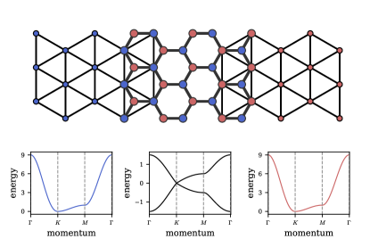
Figure 11: SUSY corresponding triangular lattices. Complex fermions (blue, left) on a triangular lattice are supersymmetrically linked to complex bosons (red, right) on the same triangular lattice. The mapping can be established with a SUSY charge which can be interpreted as the adjacency matrix of a honeycomb lattice whose two sublattices are the two triangular lattices, respectively. For the topological classification according to Table 5, we find, noting that the Witten index here is $\nu=0$, that the Dirac point at the $K$-point in the SUSY charge spectrum has a non-trivial topological invariant of $\pi_{1}=+1$.

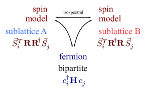
Figure 12: SUSY matching spin-spiral groundstates and free fermion Fermi surfaces. Correspondence between a bipartite fermion model and two distinct spin models on its two sublattices is shown in which the Fermi surface resembles the respective ground state manifolds of coplanar spin spirals.

Let us formulate this SUSY-perspective on the spin-fermion correspondence [78] in more mathematical terms using our previously established framework. To this end, we use the correspondence between a SUSY charge and a free chiral fermion lattice model on the lattice geometry of the SUSY charge. Such a free chiral fermion lattice model of the form

$$\mathcal{H}=\begin{pmatrix}c_{A}^{\dagger}&c_{B}^{\dagger}\end{pmatrix}\begin{pmatrix}&{\bf R}\\ {\bf R}^{\dagger}&\end{pmatrix}\begin{pmatrix}c_{A}\\ c_{B}\end{pmatrix}$$ (33)

maps onto a SUSY charge via $c_{A}\to c$ and $c_{B}\to b$. Hence, the Dirac points in the spectrum of the SUSY charge actually correspond to Dirac points in this associated fermionic Hamiltonian. Going from the SUSY charge to one of the SUSY partnering sublattices one has to square this matrix $\bf H$ yielding a block-diagonal form as in (10). In the spin-fermion correspondence, we now identify one of the two blocks ${\bf R}{\bf R}^{\dagger}$ or ${\bf R}^{\dagger}{\bf R}$ with the spin interaction matrix $\bf M$ that we diagonalize in the LT approach, as demonstrated in Fig. 12. Of course, this squaring of the original matrix has the effect that the two positive/negative energy branches of the original fermionic tight-binding model get mapped onto one another and that the Fermi energy features in the middle of the particle-hole symmetric spectrum get mapped onto the minimal energy features of the squared Hamiltonian. We have summarized this SUSY correspondence between a classical spin model on some lattice geometry with a fermionic tight-binding model on its square-root lattice in the illustration of Fig. 12 above.

Having established this SUSY framework for the spin-fermion correspondence we can return to the cases of spin models with multiple spin spiral ground states whose (sub)extensive ground-state degeneracies can be captured by some non-trivial manifold in momentum space. The first example here might be the one of face-centered cubic (fcc) lattice Heisenberg antiferromagnet, which exhibits a subextensive ground-state manifold of spin spiral states whose wavevectors constitute a line in momentum space [91], see Fig. 9. Putting our SUSY correspondence to work, we can connect this manifold to the Fermi surface of the fermionic tight-binding model on its square-root graph – the diamond lattice (with its two fcc sublattices), which indeed exhibits a line-like Fermi surface (Fig. 13).

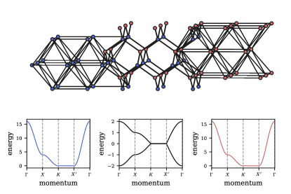
Figure 13: Spin-fermion SUSY correspondence for the fcc antiferromagnet. Complex fermions (blue, left) on the fcc lattice are supersymmetrically linked to complex bosons (red, right) on the same fcc lattice. The mapping can be established with a SUSY charge which can be interpreted as the adjacency matrix of a diamond lattice whose two sublattices are the two fcc lattices, respectively. For the topological classification according to Table 5, we find, noting that the Witten index here is $\nu=0$, that the line of Dirac points between the $K$ and $K^{\prime}$ points in the SUSY charge spectrum has a non-trivial topological invariant of $\pi_{1}=+1$ (a Berry phase of $\pi$ around the line node).

One might also be able to go one step further and construct, via our SUSY correspondence, a non-trivial spin model with a spin spiral surface describing its ground states that has hitherto not been studied. One attempt in doing so is to start from the hyperoctagon lattice geometry as SUSY charge and take its lattice square (see Fig. 14) to arrive at a three-dimensional variant of the Shastry-Sutherland model (akin to a similar SUSY connection in two spatial dimensions between the square-octagon and Shastry-Sutherland lattices exemplified in Fig. 25 of the Appendix). Since the fermionic tight-binding band structure on the hyperoctagon lattice exhibits a regular Fermi surface [92], this brings us, at first sight, to a full spin spiral surface (of codimension one) in the case of the three-dimensional Shastry-Sutherland model . Unfortunately, however, this spin spiral surface is not stable upon enforcing the Luttinger Tisza constraint, which is not fulfilled by the vast majority of k-points constituting the spin spiral surface, but only a finite set of individual points, see Fig. 15. We will leave it as an open challenge for future work to identify a nearest-neighbor Heisenberg antiferromagnet that indeed exhibits a full spin spiral surface, preferably via the SUSY correspondence at hand.

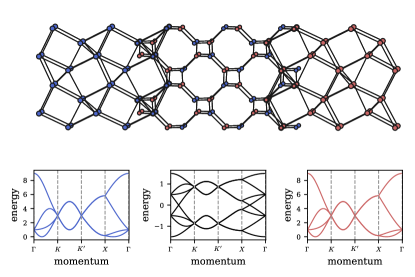
Figure 14: Spin-fermion SUSY correspondence for the three-dimensional Shastry-Sutherland antiferromagnet. Complex fermions (blue, left) on the hyperoctaon lattice (middle) are supersymmetrically linked to complex bosons (red, right) on a three-dimensional generalization of the Shastry-Sutherland lattice, see Fig. 25 in the Appendix. The ground-state manifold of spin-spiral states for this 3D Shastry-Sutherland model is illustrated in Fig. 15 below. For the topological classification according to Table 5, we find, noting that the Witten index here is $\nu=0$, that the Dirac point between the $\Gamma$ and the $K$ point and that between the $X$ and $\Gamma$ in the SUSY charge spectrum are topologically trivial (yielding a trivial $\pi_{1}$).

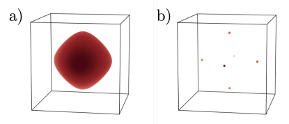
Figure 15: Spin-spiral ground-state manifold for the three-dimensional Shastry-Sutherland antiferromagnet. While the unconstrained diagonalization of the spin interaction matrix leads to a two-dimensional manifold of spin spiral states (panel a), enforcing the Luttinger-Tisza constraint reduces the actual ground states to a set of individual ${\bf k}$-points (panel b).

Finally, there is the class of $J_{1}$-$J_{2}$ Heisenberg models [81] for which the spin-fermion SUSY correspondence is particularly interesting as it seems to generically map spin systems to fermionic system with a full Fermi surface, i.e., a nodal manifold of co-dimension one. This is the case for the aforementioned $J_{1}$-$J_{2}$ model on the diamond lattice [90], a restricted $J_{1}$-$J_{2}^{*}$ model on the body-centered cubic (bcc) lattice [94, 78] or the $J_{1}$-$J_{2}$ model on the honeycomb lattice [95] where the Fermi surface (or line in the two-dimensional model) exists in various shapes and topologies for a wide range of parameters $J_{2}/J_{1}$. For the $J_{1}$-$J_{2}$ model on the fcc lattice [96, 97] one also finds a spin-spiral surface, albeit only for a single coupling parameter $J_{2}=J_{1}/2$. Conceptually, these $J_{1}$-$J_{2}$ models differ from what we have discussed so far in that they allow for couplings within the same sublattice of a bipartite lattice or are defined for a non-bipartite lattice in the first place. As such, our SUSY lattice construction which is supposed to start from a clean bipartite graph does not immediately apply. However, one can still create a proper ‘graph squaring’ in this case [78], by retaining the same lattice geometry but doubling the degrees of freedom on every site . We refer the interested reader to Ref. 78 for further details of this SUSY mapping (though the language of supersymmetry was not yet adopted in that article).

III.3 Magnon dispersions

In the third case study of our SUSY framework we will switch our attention from frustrated magnets at zero magnetic field to those in large magnetic fields. These exhibit number-conserving magnons—bosonic excitations that arise near saturation fields [99, 45, 100, 101] – and again the SUSY correspondence will reveal the existence of frustration.

Let us start with an instructive example: for the kagome antiferromagnet in a magnetic field, it has been observed that below the saturation field, localized one-magnon states populate the hexagonal motifs of the kagome lattice in the densest possible packing – a triangular magnon crystal [102, 45]. Such magnon localization is intimately related to and a precursor of the existence of the flat band in the nearby polarized state [100]. Here we explain the existence of the flat band using our SUSY framework: the magnons have a SUSY partner on the honeycomb lattice. We will, in a first step, construct the fermionic analog of such a (topological) magnon spectrum. Reverting this procedure in a second step, we demonstrate how one can then predict non-trivial magnon phenomenology from their fermionic SUSY partners.

To accomplish the first step, going from a bosonic magnon dispersions to its SUSY fermionic counterpart, we again return to our principal example of the honeycomb-kagome correspondence from the introduction (Fig. 1). Here we start on the kagome side and consider a spin-$S$ kagome Heisenberg antiferromagnet subject to a uniform magnetic field $h>0$

$${\cal H}=J\sum_{\langle i,j\rangle}{\bf S}_{i}\cdot{\bf S}_{j}-h\sum_{i}S_{i}^{z}\,.$$ (34)

At high fields, beyond a saturation value of $h=6JS$, the ground state is a fully polarized state [99, 45, 46]. To obtain the excitation spectrum of magnons in this phase we express the on-site spin operators $S^{\pm}_{j}=S^{x}_{j}{\pm}iS^{y}_{j}$ and $S^{z}_{j}$ in terms of bosonic (magnon) annihilation and creation operators $b_{j}$ and $b_{j}^{\dagger}$ following the Holstein-Primakoff expansion of (28). Keeping up to terms quadratic in the bosonic operators in the large-$S$ limit (assuming $h\propto S$), we arrive at a bosonic tight-binding Hamiltonian on the kagome lattice

$${\cal H}^{\text{sw}}_{ij}=JS\sum_{\langle i,j\rangle}\left(b_{i}^{\dagger}b_{j}^{\phantom{\dagger}}+{\rm h.c.}\right)+(h-4JS)\sum_{i}n_{i}\,,$$ (35)

with a hopping of strength $JS$ and chemical potential $(h-4JS)$. Translating to Fourier space, the corresponding Bloch Hamiltonian reads

$$H^{B}_{ij}({\bf k})=h-4JS+\\ S\sum_{\bf L}J_{\text{kagome}}({\bf d}_{i}-{\bf d}_{j}-{\bf L})e^{i{\bf k}\cdot({\bf d}_{i}-{\bf d}_{j}-{\bf L})}$$ (36)

where $J_{\text{kagome}}(\delta{\bf r})=J$ if $\delta{\bf r}$ represents a nearest neighbor separation on the kagome lattice with basis vectors ${\bf d}_{i}$ and Bravais lattice vectors ${\bf L}$ and zero otherwise. The spectrum consists of a flat branch of magnons at $\omega_{\bf k}=h-6JS$ and two dispersive branches at $\omega_{\bf k}=h-3JS\pm JS\sqrt{3+2\sum_{i}\cos({{\bf k}\cdot{\bf d}_{i}})}$ identical to Fig. 1 on the kagome side shifted by a constant $(h-6JS)$ (to obtain exactly the same spectrum, set the field to exactly the point of saturation $h=6JS$). This high-field limit of a frustrated kagome Heisenberg antiferromagnet, therefore, provides us with a natural setup to realize the simplest tight-binding model of bosons on the kagome lattice.

Let us now proceed to explicitly construct its fermionic partner, which via our SUSY lattice correspondence we expect to live on the honeycomb lattice and be exactly isospectral to the bosonic kagome model (up to flat bands). Our starting point is the magnon Hamiltonian $H_{B}({\bf k})$ in (36), where for simplicity we set the magnetic field to the point of saturation $h=6JS$ to bring the lowest eigenvalue of $H_{B}({\bf k})$, the flat band, to $\omega_{\bf k}=0$. The crucial step then is to construct the supercharge matrix ${\bf R}$ of (3) by factorizing $H_{B}({\bf k})$ in (36) as $H_{B}({\bf k})={\bf R}^{\dagger}({\bf k}){\bf R}({\bf k})$. To keep in mind, such a decomposition should preserve the locality of $H_{B}({\bf k})$, namely, if $H_{B}({\bf k})$ consists only of nearest-neighbor hoppings, so should be reflected in the connectivities of ${\bf R}({\bf k})$. This would then yield a local fermion model with preserved topological signatures such as localized edge modes if the bosonic side has any.

In essence, the factorization is tantamount to the square-rooting of $H_{B}({\bf k})$. We could produce this factorization using the graph square-rooting algorithm of Appendix A. But instead we can also draw insights from our graph correspondence — one may opt for a decomposition such that ${\bf R}({\bf k})$ is a rectangular matrix. Specifically, for the kagome-honeycomb case, it is a $2\times 3$ matrix as the partner lattice of kagome is the honeycomb lattice (Fig. 1). This implies the Witten index is $\nu=1$ and there is a flat band on the kagome side.

Empowered with the knowledge of this graph correspondence, we first identify the supercharge matrix ${\bf R}({\bf k})$. Introducing lower case indexing for the bosonic lattice and upper case indexing for the fermionic lattice, we can express it as

$${\bf R}_{Ij}({\bf k})=\\ \sqrt{S}\sum_{\bf L}J_{\text{honeycomb-X}}({\bf n}_{I}-{\bf d}_{j}-{\bf L})e^{i{\bf k}\cdot({\bf n}_{I}-{\bf d}_{j}-{\bf L})}\,,$$ (37)

where $J_{\text{honeycomb-X}}(\delta{\bf r})=\sqrt{J}$ if $\delta{\bf r}$ is a nearest neighbor separation on the honeycomb-X lattice with honeycomb basis vectors ${\bf n}_{I}$ and zero otherwise. Together ${\bf d}_{i}$ and ${\bf n}_{I}$ form the basis of the bipartite honeycomb-X lattice.

Please note the simplicity of the step from (36) to (37) arises from the choice of the “canonical gauge” where the Fourier transform is taken with the site locations $e^{i{\bf k}\cdot{\bf r}}$ and not the “periodic gauge” where it is taken with the unit cell location $e^{i{\bf k}\cdot{\bf R}}$ [103]. If preferred, one can always switch to the periodic gauge after the Hamiltonians are identified.

The superpartner of the magnon model, e.g., the fermionic Hamiltonian then derives by noting its Bloch form $H_{F}({\bf k})={\bf R}({\bf k}){\bf R}^{\dagger}({\bf k})$ which reads

$$H^{F}_{IJ}({\bf k})=3JS+\\ S\sum_{\bf L}J_{\text{honeycomb}}({\bf n}_{I}-{\bf n}_{J}-{\bf L})e^{i{\bf k}\cdot({\bf n}_{I}-{\bf n}_{J}-{\bf L})}\,,$$ (38)

where $J_{\text{honeycomb}}(\delta{\bf r})=J$ if $\delta{\bf r}$ connect nearest neighbors on the honeycomb lattice and zero otherwise. This Hamiltonian has an identical spectrum as the magnons but the flat band. We immediately recognize that this fermionic model represents the well-known Dirac semimetal on the honeycomb lattice.

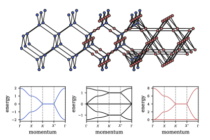
Figure 16: Diamond-pyrochlore SUSY correspondence. Complex fermions (blue, left) on the diamond lattice are supersymmetrically linked to complex bosons (red, right) on the pyrochlore lattice. The middle panel shows the band structure of the SUSY charge lattice Hamiltonian on the diamond-X lattice. For the topological classification according to Table 1, we find, noting that the Witten index here is $\nu=2$, that the nexus point in the SUSY charge spectrum has a non-trivial topological invariant of $\pi_{2}=-1$, see also the illustration in Fig. 23 of the Appendix.

In summary, magnons described by a kagome Heisenberg model at saturation field have a fermionic partner with an index of $\nu=1$ demanding a flat band in their spectrum. This would seem like a complex procedure to discover a flat band, but it has an important benefit: it implies that a Heisenberg model on any example illustrated in the triptych-like figures of Section III that exhibits a non-zero Witten index $\nu\neq 0$ leads to a magnon dispersion with a flat band in a saturation field – and thereby constitutes a candidate system for a magnon crystal just below saturation. This allows us to go well beyond the known cases of kagome [100] and pyrochlore [101] antiferromagnets and postulate magnon crystals just below the saturation field, for instance, also for the squagome and the hyperkagome antiferromagnets along with a number of other two- and three-dimensional systems.

III.4 Parton dispersions

The phenomenon of displaying identical band structures by virtue of a graph correspondence finds realization in other frustrated magnets as well, specifically, in quantum spin liquid (QSL) that have been discussed in certain spin-orbit coupled materials. Such QSL are unconventional phases of matter with one characteristic being the emergence of fractional excitations, called partons, instead of more conventional magnons (as discussed above) or electronic quasiparticles. Depending on the underlying effective microscopic descriptions, the partons can range from being Abrikosov spinons [104], which are charge-neutral complex fermions carrying spin $S=1/2$, to Majorana fermions [105, 106], which are also charge neutral but do not carry any spin quantum number. While it remains an interesting open question if one can construct an exact SUSY mapping between different types of partons, we observe a curious similarity between the respective parton dispersions in two such distinct types of QSLs: One that features a spinon Fermi surface of gapless Abrikosov spinons coupled to $U(1)$ gauge fields [107], and the other that features a Majorana Fermi surface of Majorana fermions coupled to $\mathbb{Z}_{2}$ gauge fields [108]. This identification turns out to ensue from the same type of graph correspondence that we have been discussing in our SUSY construction, but now between the underlying lattice geometries that harbor the QSLs. In other words, the graph correspondence enlightens the fact that the hopping Hamiltonians of partons on these two lattices must be isospectral (except for possible flat bands which do not play a substantial role here).

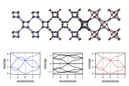
Figure 17: Hyperoctagon-hyperkagome SUSY correspondence. Complex fermions (blue, left) on the hyperoctagon lattice are supersymmetrically linked to complex bosons (red, right) on the hyperkagome lattice. The middle panel shows the band structure of the SUSY charge lattice Hamiltonian on the hyperoctagon-X lattice. For the topological classification according to Table 1, we find, noting that the Witten index here is $\nu=2$, that the nexus point in the SUSY charge spectrum has a non-trivial topological invariant of $\pi_{2}=+1$, see also the illustration in Fig. 23 of the Appendix.

The $U(1)$ QSL has been discussed in the context of a Heisenberg model on the hyperkagome lattice [107], after experimental indications of spin liquid behavior were reported for the hyperkagome iridate compound Na₄Ir₃O₈ [109]. Via our graph correspondence the spinon spectrum of this $U(1)$ QSL can be identified with the Majorana spectrum of a $\mathbb{Z}_{2}$ QSL emerging in a three-dimensional Kitaev model on the hyperoctagon lattice [108] whose Hamiltonian consists of characterisitic bond-directional Ising-like spin exchanges [110]. Both of these lattices, the hyperkagome and the hyperoctagon, can be obtained from our previous examples of the pyrochlore and the diamond lattice with a suitable depletion of tetrahedra or bonds, respectively, but more importantly in our context here, also from one another – the hyperoctagaon lattice is the premedial lattice of the hyperkagome lattice [108]. That is, one obtains the hyperoctagon structure by shrinking each triangle of the hyperkagome lattice to a single vertex and respecting the connectivity of the original corner-sharing triangles – but this is precisely the lattice square-rooting procedure of our SUSY lattice correspondence (Fig. 2). Identifying these two lattice geometries as superpartners, we can also quickly construct the lattice of the supercharge that mediates the transformation between the two – the hyperoctagon-X lattice illustrated in the middle of Fig. 17. The graph correspondence thus implies that the spinon excitation spectrum in the hyperkagome lattice has a bosonic partner on the hyperoctagon lattice. Suprisingly, however, we find it also coincides with the Majorana excitation spectrum on the same hyperoctagon lattice. It turns out, the real symmetric hopping matrix of the bosons is gauge equivalent via $b_{j}\to ib_{j},j\in$ sublattice $A$ to the real antisymmetric hopping matrix of the Majorana fermions on the bipartite hyperoctagon lattice. Hence, both feature extended two-dimensional Fermi surfaces around the point of isotropic hoppings of the fermions on the individual lattices . We have thus connected two enigmatic QSLs discussed in the literature via our SUSY framework.

We will return to Kitaev QSLs in Section IV, where we will exploit the fact that they can be cast in terms of free Majorana fermion models to formulate a SUSY connection to real bosons and their classical analogs to discuss mechanical incarnations of Kitaev spin liquid physics.

IV Topological mechanics

We now turn to the second broader context in which we can apply our SUSY framework to establish connections between two seemingly distant fields – topological mechanics and the physics of Majorana fermions. It rests on the principal observation that mechanical systems evolve around phase space coordinates $(q,p)$, i.e., the classical limit of real bosonic degrees of freedom whose most natural SUSY partners are real (Majorana) fermions. On a technical level, this will require us to expand our SUSY correspondence, which we had presented for the case of complex bosons and fermions in Section II, to the case of real bosons and fermions. We will see this also has implications on the accompanying SUSY lattice correspondence.

Since the dynamics in mechanical setups is generally time-reversal symmetric and our SUSY correspondence respects this symmetry (as in the complex case), a natural starting point on the fermionic side is to consider time-reversal symmetric Majorana Hamiltonians. In the parlance of symmetry classes, the latter belong to symmetry class BDI in the ten-fold way [36, 21] and admit a block-off-diagonal form as in (1) when expressed in a suitable basis. As we will discuss in the following (Section IV.1), this matrix form implies that it is always possible to construct a local supercharge that generates a representative fermion Hamiltonian from this class [112]. The locality is crucial in preserving the topology of the models identified by SUSY, i.e., to carry over to the bosonic side. We demonstrate that this procedure is not only a natural connection between real fermions and bosons but offers another important reward – the canonically conjugate positions and momenta get decoupled in the resultant bosonic Hamiltonian, crucially allowing us to formulate classical analogs in terms of balls-and-springs networks. SUSY thus paves a way to construct proper mechanical analogs of Majorana models that can be studied in table-top experiments. Notably, these mechanical systems will exhibit a topological response protected by SUSY, if the fermionic partner system has any. Principal examples, which we will present in the following, will include mechanical analogs of topological superconductors (in Section IV.2), Kitaev spin liquids (in Section IV.3), and higher order topological insulators (in Section IV.4).

Let us finally note that the discussion in this section is based on an earlier short paper by our collaboration [15], but it goes beyond the previous work by putting it into the context of the unifying SUSY framework developed in this manuscript.

IV.1 SUSY mapping for real fermions and bosons

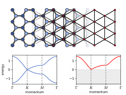
Figure 18: SUSY correspondence for real fermions and bosons. Real (Majorana) fermions on a bipartite lattice (such as the honeycomb lattice on the left) have an isospectral SUSY partner in the form of real bosons on one of its sublattices (such as the triangular lattice on right). Eigenmodes in these systems, depicted in the lower panels, agree for all non-negative energies, including potential zero modes.

We set out by recasting the SUSY formalism, outlined in Section II.1 for complex fermions and bosons, to their real counterparts. Our starting point will be a model system on the fermionic side, i.e., a Majorana fermion hopping model, that we define on a bipartite lattice such as the honeycomb lattice depicted on the left in Fig. 18. Note that this choice of a bipartite lattice for the fermionic side is a first distinction to the complex SUSY scenario where we did not make such a restriction. Adapting a suitable basis, one can cast such a Majorana Hamiltonian on any given bipartite lattice into a block off-diagonal form

$${\cal H}_{F} ={-\frac{i}{2}}\gamma^{A}_{i}{\bf A}_{ij}\gamma^{B}_{j}+{\rm h.c.}\,,$$

$$={\frac{i}{2}}\begin{pmatrix}\gamma^{A}&\gamma^{B}\end{pmatrix}\begin{pmatrix}&-{\bf A}\,\,\\ {\bf A}^{T}&\end{pmatrix}\begin{pmatrix}\gamma^{A}\\ \gamma^{B}\end{pmatrix}\,,$$ (39)

where the matrix ${\bf A}$ represents the lattice adjacencies (or connections between the sublattices $A$ and $B$) weighted by appropriate hopping strengths and the $\gamma^{A}$ and $\gamma^{B}$ are the Majorana creation/annihilation operators that reside on the two sublattices. We now want this Hamiltonian to be the fermionic component of a SUSY Hamiltonian ${\cal H}_{\rm SUSY}=\frac{1}{2}\{\mathcal{Q},\mathcal{Q}^{\dagger}\}$, generated by a supercharge ${\cal Q}$. To this end, let us consider the Hermitian supercharge

$${\cal Q} =\gamma^{A}_{i}{\bf A}_{ij}{\hat{q}}_{j}+\gamma^{B}_{i}{\bf 1}_{ij}{\hat{p}}_{j}\,,$$

$$=\begin{pmatrix}\gamma^{A}&\gamma^{B}\end{pmatrix}\begin{pmatrix}{\bf A}&\\ &{\mathbf{1}}\end{pmatrix}\begin{pmatrix}\hat{q}\\ \hat{p}\end{pmatrix}\,,$$ (40)

which connects the Majorana fermion operators $\gamma^{A}$ and $\gamma^{B}$ (on the two sublattices of the fermionic lattice) to real bosonic operators $\hat{q}$ and $\hat{p}$, which equal in number and conjugate to one another. The SUSY Hamiltonian of this Hermitian supercharge ${\cal H}_{\rm SUSY}={\cal Q}^{2}\equiv{\cal H}_{F}+{\cal H}_{B}$ then block-decomposes into a fermionic and bosonic part. The resultant bosonic Hamiltonian, in terms of the variables $(\hat{q},{\hat{p}})$ reads

$${\cal H}_{B} ={\frac{1}{2}}\sum_{ij}{\hat{q}}_{i}({\bf A}^{T}{\bf A})_{ij}{\hat{q}}_{j}+\frac{1}{2}\sum_{i}\hat{p}_{i}\hat{p}_{i}\,,$$

$$={\frac{1}{2}}\begin{pmatrix}\hat{q}&\hat{p}\end{pmatrix}\begin{pmatrix}{\bf A}^{T}{\bf A}&\\ &{\mathbf{1}}\end{pmatrix}\begin{pmatrix}\hat{q}\\ \hat{p}\end{pmatrix}.$$ (41)

Before we further inspect this bosonic Hamiltonian let us first point out a few noteworthy features that distinguishes the construction so far from the complex case and, in particular, the lattice correspondence expounded before. First, let us introduce, in analogy to our discussion of complex fermion-boson SUSY in Section III, the matrix

$${\bf R}=\begin{pmatrix}{\bf A}&\\ &{\mathbf{1}}\end{pmatrix}\,,$$ (42)

which is representative of the supercharge ${\cal Q}$. In the real case discussed here, it is block-diagonal. Moreover, in the complex case, following the interpretation of the SUSY in terms of a graph correspondence, the fermionic and the bosonic models were defined on the two sublattices of a bipartite lattice (which we identified with the SUSY charge). The real case is strikingly different in this context: It is the Majorana fermions that now span the entire bipartite lattice under consideration, while their bosonic partners inhabit only one of its sublattices. This is visualized in Fig. 18 where we start with a Majorana fermion model on the honeycomb lattice (left) and end up with bosonic degrees of freedom that live on one of its two triangular sublattices (right). Technically, it is sublattice $B$ by virtue of the construction of ${\cal Q}$ in (IV.1) . We have schematically summarized this SUSY correspondence between Majorana fermions and real bosons and their lattice correspondence in Fig. 19.

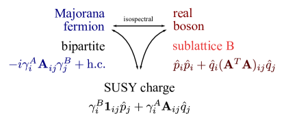
Figure 19: SUSY correspondence of real bosons and Majorana fermions. Schematic relation between real bosons and Majorana fermions. Here, the real bosons reside on the sublattice of the bipartite Majorana fermion lattice.

The spectral identification induced by the supercharge ${\cal Q}$ of (IV.1) is subtle and distinct from the complex case. For the complex case, we had isospectrality between two Hermitian matrices, the two Bloch Hamiltonians ${\bf R}{\bf R}^{\dagger}$ and ${\bf R}^{\dagger}{\bf R}$. In the real case, the excitation spectra of ${\cal H}_{F}$ and ${\cal H}_{B}$ are obtained from the respective equations of motion in the Fourier space

$$\frac{\rm d}{{\rm d}t}\begin{pmatrix}{\gamma}_{A}\\ {\gamma}_{B}\end{pmatrix} =i\begin{pmatrix}&-{\bf A}({\bf k})\\ {\bf A}^{\dagger}({\bf k})&\end{pmatrix}\begin{pmatrix}\gamma_{A}\\ \gamma_{B}\end{pmatrix}\,,$$

$$\frac{\rm d}{{\rm d}t}\begin{pmatrix}{\hat{p}}\\ {\hat{q}}\end{pmatrix} =i\begin{pmatrix}&-1\\ {\bf A}^{\dagger}({\bf k}){\bf A}({\bf k})&\end{pmatrix}\begin{pmatrix}\hat{p}\\ \hat{q}\end{pmatrix}\,,$$ (43)

and diagonalizing the matrices on the right hand side which are known as the Lie generators [114]. In a compact form, the fermionic and the bosonic Lie generators read respectively as

$${\cal L}_{F}={\bf R}({\bf k})\sigma_{2}{\bf R}^{\dagger}({\bf k})\quad{\rm and}\quad{\cal L}_{B}=\sigma_{2}{\bf R}^{\dagger})({\bf k}){\bf R})({\bf k})\,,$$

where $\sigma_{2}$ is an extension of the Pauli matrix in the enlarged space of dimension $2N$ for $N$ number of operators of each flavor (both fermionic and bosonic) in the unit cell or equivalently, $2N$ sites in the unit cell. The forms of the two Lie generators suggest they are isospectral, again except for zero modes, with the excitation spectrum in the bosonic model being identified with the positive branch of the eigenvalues of ${\cal L}_{B}$, see the bottom panels of Fig. 18 for our example system.

Classical limit

We note that all the operators in our discussion above are quantum mechanical ones. In the appropriate classical limit, the boson Hamiltonian in (IV.1) represents a mechanical analog of the Majorana Hamiltonian in (IV.1) in terms of a balls-and-springs model. Without loss of generality, we can assume the balls to be of unit masses with their dynamics described by the classical Hamiltonian

$${\cal H}_{\rm cl} =\frac{1}{2}\sum_{m}e^{2}_{m}+\frac{1}{2}\sum_{i}p^{2}_{i}$$

$$=\frac{1}{2}\sum_{ij}q_{i}({\bf A}^{T}{\bf A})_{ij}q_{j}+\frac{1}{2}\sum_{i}p^{2}_{i}\,.$$ (44)

In the first line of the above equation, the spring extensions are denoted by $\{e_{m}\}$ which can be linearized in terms of the coordinates of the balls, $\{q^{i}\}$ via $e_{m}={\bf A}_{mi}q^{i}$ introducing a compatibility matrix ${\bf A}$. The matrix ${\bf R}$, introduced in (42), extends this to accommodate all bosonic degrees of freedom $\{(q^{i},p_{i})\}$ and is referred to as the rigidity matrix of the mechanical system. It thereby also renders a physical meaning to the SUSY charge (IV.1) of our construction.

Reexpressing the classical Hamiltonian in (IV.1) as

$${\cal H}_{\rm cl} =\sum_{ij}\frac{k_{ij}}{2}(q_{i}-q_{j})^{2}+\sum_{i}\frac{\kappa_{i}}{2}q^{2}_{i}+\frac{1}{2}\sum_{i}p^{2}_{i}\,,$$ (45)

we observe the mechanical model comprises both intersite and onsite springs of spring constants $k_{ij}$ and $\kappa_{i}$ respectively. Their parametric dependence can be read off as [15]

$$k_{ij} =-\sum_{a\in A}{\bf A}^{T}_{ia}{\bf A}_{aj},$$ (46)

$$\kappa_{i} =\sum_{a\in A}{\bf A}^{2}_{ia}-\sum_{b\in B}k_{ib}\,,$$ (47)

where $k_{ij}$ are the off-diagonal elements of ${\bf A}^{T}{\bf A}$, that, by virtue of our SUSY construction, arise from the next-nearest-neighbor Majorana hopping (within the boson sublattice $B$) and $\kappa_{i}$ are the diagonal elements of ${\bf A}^{T}{\bf A}$ arising from the Majoranas hopping back and forth, modified by a contribution coming from the intersite springs. The matrix

$${\bf D}={\bf A}^{T}{\bf A}$$

is known as the dynamical matrix of the mechanical model.

The normal mode frequencies are obtained from the square-root of the eigenvalues of ${\bf D}$, however, the normal modes are not the eigenstates of ${\bf D}$. As described in the previous section, they are instead obtained by diagonalizing the Lie generator ${\cal L}_{B}$ of the equations of motion (IV.1). The positive branch of the eigenvalues of ${\cal L}_{B}$ coincides with the square-rooted eigenvalues of ${\bf D}$. In the following, we will unfold the topology associated with these normal modes in periodic systems.

Topology of real bosons

Previously in Section II, we identified the topological invariants to classify the band topology in quadratic systems of complex fermions and bosons that are related by SUSY. We revisit this here for the real case to illuminate the same for the normal modes in mechanical systems and unveil new topological invariants.

We first need to settle the relationship between the real and complex formalisms. The Hermitian SUSY charge discussed in the previous sections, such as in (IV.1), is focused on the BDI class. The general form is ${\cal Q}=\gamma{\bf R}{\bf x}$ where we combine the canonical coordinates into one vector ${\bf x}=(\hat{q},\hat{p})^{T}$ and have not placed any restrictions on ${\bf R}$ so that it describes a system with no symmetry. Written this way, the matrix ${\bf R}$ is a general real rectangular matrix but now appears double the size of the corresponding matrix in the complex formalism (II.4). Switching from real to complex veriables then produces a SUSY charge of the form

$${\cal Q}_{\rm SF}=\begin{pmatrix}c^{\dagger}&c\end{pmatrix}\begin{pmatrix}{\bf R}_{1}&{\bf R}_{2}\\ {\bf R}_{2}^{*}&{\bf R}_{1}^{*}\end{pmatrix}\begin{pmatrix}b\\ b^{\dagger}\end{pmatrix}\,.$$ (48)

So this doubling turns out to exactly match the Hermitian part of Eq. (29) in our example from geometrically frustrated magnets in Section III.1. Hence, a change of variables from real to complex reveals indeed ${\cal Q}={\cal Q}_{\rm SF}$. But we also see that at a matrix level, obtained by writing

$${\cal Q}=\frac{1}{2}\begin{pmatrix}\bm{\gamma}&{\bf x}\end{pmatrix}\begin{pmatrix}&{\bf R}\\ {\bf R}^{T}&\end{pmatrix}\begin{pmatrix}\bm{\gamma}\\ {\bf x}\end{pmatrix},$$ (49)

and writing ${\cal Q}_{\rm SF}$ in a similar way with spinor $(c,c^{\dagger},b,b^{\dagger})^{T}$, the topological class of ${\cal Q}$ and ${\cal Q}_{\rm SF}$ are the same, class BDI. Even though there is no physical symmetry in the real formalism beyond fermion parity, the matrix as viewed by the topological class has both ${\cal T}$ and ${\cal P}$ symmetry. So the topological properties in the real formalism can readily be understood just by directly classifying the matrix defining the quadratic real SUSY charge.

The use of the real formalism comes with a benefit: their Berry curvature signals a topological non-trivial system. To understand this, we need to step back and consider a subtlety of the real-formalism.

The SUSY charge for the complex case identifies individual fermionic eigenstates with their bosonic partners at equal (nonzero) energies as in (13), thereby connecting the two Hilbert spaces. What demarcates the real case is that such a spectral identification, instead of two Hamiltonians, applies to the two Lie generators ${\cal L}_{F}$ and ${\cal L}_{B}$ in (IV.1). While ${\cal L}_{F}$ turns out to be the Majorana Hamiltonian itself and therefore a Hermitian operator, ${\cal L}_{B}$ is a Krein-Hermitian operator satisfying $\sigma_{2}{\cal L}_{B}={\cal L}_{B}^{\dagger}\sigma_{2}$ [115, 116]. Accordingly, the bosonic normal modes obtained by diagonalizing ${\cal L}_{B}$ obey $\langle v_{m}|\sigma_{2}|v_{n}\rangle=[\sigma_{3}]_{m,n}$ while the fermionic ones, obtained by diagonalizing ${\cal L}_{F}$, obey $\langle u_{m}|u_{n}\rangle=\delta_{m,n}$. In other words, for the real case, the supercharge relates the members (the fermionic states) of a Hilbert space to those (the bosonic states) of a Krein space.

With the classification and Lie generator eigenvalue problems in mind, the SUSY map, discussed in Section II.4 in (14), implies a constraint on the Berry phases associated with the same band in each of the three SUSY eigenproblems

$$\theta_{F}^{(m)}=\theta_{B}^{(m)}+\theta_{\cal Q}^{(m)}\,.$$ (50)

This constraint is readily determined by expressing for example the fermionic states $|u_{m}({\bf k})\rangle$ that are eigenvectors of ${\cal L}_{F}$ in the Berry phase $\theta^{(m)}_{F}$ in terms of the bosonic eigenstates $|v_{m}({\bf k})\rangle$ that are Krein space eigenvectors of ${\cal L}_{B}$. Doing so leads to the relation

$$i\oint\langle u_{m}({\bf k})|\partial_{\bf k}u_{m}({\bf k})\rangle\cdot{\rm d}{\bf k}=i\oint\langle v_{m}({\bf k})|\sigma_{2}|\partial_{\bf k}v_{m}({\bf k})\rangle\cdot{\rm d}{\bf k}$$

$$\leavevmode\nobreak\ \leavevmode\nobreak\ \leavevmode\nobreak\ \leavevmode\nobreak\ \leavevmode\nobreak\ \leavevmode\nobreak\ \leavevmode\nobreak\ \leavevmode\nobreak\ \leavevmode\nobreak\ \leavevmode\nobreak\ \leavevmode\nobreak\ \leavevmode\nobreak\ \leavevmode\nobreak\ \leavevmode\nobreak\ \leavevmode\nobreak\ \leavevmode\nobreak\ \leavevmode\nobreak\ \leavevmode\nobreak\ \leavevmode\nobreak\ \leavevmode\nobreak\ \leavevmode\nobreak\ \leavevmode\nobreak\ \leavevmode\nobreak\ \leavevmode\nobreak\ +\oint\frac{{\rm Im}\left(\langle u_{m}({\bf k})|(\partial_{\bf k}{\bf R})|v_{m}({\bf k})\rangle\right)}{\sqrt{\omega_{m}({\bf k})}}\cdot{\rm d}{\bf k}\,,$$ (51)

where we identify the third term as the Berry phase of an eigenvalue problem associated with the SUSY charge ${\bf Q}$ (not discussed).

This constraint allows for an alternative interpretation of the protection of zero modes in a SUSY system, as the constraint itself implies the existence of an alternative Berry potential. For the bosonic system, this SUSY Berry potential can be written as

$${\cal A}^{(m)}_{\rm SUSY}=\langle v_{m}({\bf k})|i\sigma_{2}(\nabla_{\bf k}+\sigma_{2}\tilde{\bf R}^{\dagger}\nabla_{\bf k}\tilde{\bf R})|v_{m}({\bf k})\rangle,$$ (52)

where the single-particle bosonic state $|v_{m}({\bf k})\rangle$ is an eigenstate of ${\cal L}_{B}$ at energy $\omega_{m}({\bf k})$ (a similar statement is readily made for the fermionic system). ${\cal A}^{(m)}_{\rm SUSY}$ is mathematically identical to the fermionic Berry potential that gives rise to $\theta^{(m)}_{F}$ but defined entirely by the bosonic eigenvalue problem and the ${\bf R}$ matrix. Therefore, SUSY reveals an additional covariant derivative term on top of the conventional bosonic Berry connection $\langle v_{m}({\bf k})|i\sigma_{2}|\nabla_{\bf k}v_{m}({\bf k})\rangle$. The constraint of (50) allows a bosonic system to inherit the Berry phase of the SUSY related fermionic system (and vice versa).

The above perspective allows us to define the bosonic Berry phase in supersymmetric systems in an alternate way

$$\theta_{B,{\rm SUSY}}^{(m)}=\oint{\cal A}_{\rm SUSY}^{(m)}\cdot{\rm d}{\bf k}\,,$$ (53)

which can indeed reveal nontrivial windings $w\equiv\theta_{B}^{(m)}/\pi$ for the nodal points or lines in the spectrum of the normal modes in a topological mechanical system—examples of which will follow in the next Sections. Similar to the case of complex fermions and bosons presented in Appendix E, the supersymmetric version of the Berry curvature for a mechanical system will follow from ${\cal F}^{(m)}_{\rm SUSY}=\nabla\times{\cal A}^{(m)}_{\rm SUSY}$ and will be useful in exploring the topology of Chern bands in apposite setups.

This discussion brings the SUSY formulation of topological mechanics to a special footing compared to the complex fermion-boson correspondence, where all our examples featured, in contrast to what has been discussed here, identical Berry phases and curvatures rendering a vanishing SUSY contribution to the underlying Berry connection (see again Appendix E). In the mechanical systems, the topology in the bosonic models is revealed by the supersymmetric Berry potential in (52) while the conventional definition of the Berry connection signals merely a trivial phase.

In the following, we will discuss one- and two-dimensional examples of mechanical systems which are the supersymmetric partner of the Kitaev chain, the Kitaev honeycomb spin liquid and a higher-order topological insulator of Majorana fermions.

IV.2 Mechanical analog of the Kitaev chain:
the Kane-Lubensky chain

In their groundbreaking paper on topological mechanics [7], Kane and Lubensky contemplated a mechanical analog of the Su–Schrieffer–Heeger (SSH) model by constructing a chain of rotors connected by springs with a dimerized unit cell, i.e., two rotors per unit cell, as illustrated on the right of Fig. 20. This is an example of an isostatic mechanical frame where the number of constraints matches the number of degrees of freedom in the system. The SSH model [117] itself constitutes what in today’s terms is the first example of fermionic topological bands with gapless edge modes arising from a bulk-edge correspondence [55]. Analogously, the mechanical model supports zero modes at the boundary for specific configurations in the parameter space when small angular dispacements around a dimerized configuration of the rotors are connected to the spring lengths $l_{n}={\bf A}_{ni}\theta_{i}$ ($\bf A$ being the compatibility matrix). For a periodic chain with uniform rotors (of radius $r$, separated by a distance $a$), one can work in Fourier space to obtain [118]

$${\bf A}(k)=\begin{pmatrix}q_{+}&q_{-}\\ q_{-}&q_{+}e^{ik(2a)}\end{pmatrix},$$ (54)

where $q_{\pm}=r\cos{\bar{\theta}}(2r\sin{\bar{\theta}}\pm a)/\sqrt{a^{2}+4r^{2}\cos^{2}{\bar{\theta}}}$, $\bar{\theta}$ (the angular deviation from a vertical axis) specifying the dimerized configuration as in Fig. 20.

The normal mode frequencies are obtained from the square-root of the eigenvalues of the dynamical matrix ${\bf D}(k)={\bf A}^{\dagger}{\bf A}$ (a representative spectrum shown in Fig. 20 with red solid lines for $r/a=0.5,\bar{\theta}=0.1$). In real space, for a chain of $N$ rotors, the dynamical matrix ${\bf D}={\bf A}^{T}{\bf A}$ is an $N\times N$ matrix of the form

$${\bf D}=\begin{pmatrix}q_{+}^{2}&q_{-}^{2}&0&0&\dots&q_{-}^{2}\\ q_{-}^{2}&q_{+}^{2}&q_{-}^{2}&0&\dots&0\\ 0&q_{-}^{2}&q_{+}^{2}&q_{-}^{2}&\dots&0\\ \vdots&\vdots&\vdots&\vdots&\vdots&\vdots\\ 0&0&\dots&q_{-}^{2}&q_{+}^{2}&q_{-}^{2}\\ q_{-}^{2}&0&0&\dots&q_{-}^{2}&q_{+}^{2}\end{pmatrix}.$$ (55)

Applying our SUSY correspondence, one can recognize the superpartner of this mechanical model is the Kitaev chain [119] with the two hoppings specified by $q_{\pm}$. As on the mechanical/bosonic side, the chain is dimerized, we obtain a 4-site unit cell for the fermion model. The spectrum is shown in Fig. 20 with blue solid lines (for $r/a=0.5,\bar{\theta}=0.1$) which is periodic over $k\in[-\pi/2,\pi/2]$ due to the unit-cell doubling.

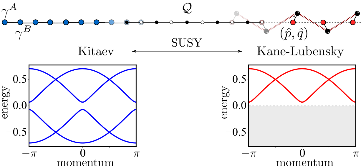
Figure 20: SUSY between the Kane-Lubensky chain and the Kitaev chain. The superpartner of the Kitaev Majorana chain (left) is the Kane-Lubensky chain (right) of mechanical rotors. The dimerization of the Kane-Lubensky chain requires doubling the unit cell of the Kitaev chain. SUSY identifies the positive branch of the spectra on both sides.

As an important extension, next we demonstrate how one can construct a random Kitaev chain from a random one-dimensional phonon problem at the isostatic point identifying the two as superpartners of each other. For this, we consider a random $N\times N$ dynamical matrix which is structurally similar to the Kane-Lubensky dynamical matrix in (55) in terms of connectivities and can be expressed as

$$\tilde{\bf D}=\begin{pmatrix}a&b&0&0&\dots&b\\ b&a&b&0&\dots&0\\ 0&b&a&b&\dots&0\\ \vdots&\vdots&\vdots&\vdots&\vdots&\vdots\\ 0&0&\dots&b&a&b\\ b&0&0&\dots&b&a\end{pmatrix}.$$ (56)

Here $a,b$ are coupling parameters of the phonon model assuming random values unlike the Kane-Lubensky chain where they were specific functions of $r,a,\bar{\theta}$ .

To construct the fermionic model, one requires to identify a supercharge or equivalently, to derive a random compatibility matrix $\tilde{\bf A}$ from the dynamical matrix $\tilde{\bf D}$ such that $\tilde{\bf D}=\tilde{\bf A}^{T}\tilde{\bf A}$. It turns out that, for this one-dimensional problem, such a decomposition is indeed possible where the matrix $\tilde{\bf A}$ maintains the same degree of locality as $\tilde{\bf D}$ in terms of the connectivities and assumes an $N\times N$ form

$$\tilde{\bf A}=\begin{pmatrix}b_{1}&b_{2}&0&0&\dots&0\\ 0&b_{1}&b_{2}&0&\dots&0\\ 0&0&b_{1}&b_{2}&\dots&0\\ \vdots&\vdots&\vdots&\vdots&\vdots&\vdots\\ 0&0&\dots&0&b_{1}&b_{2}\\ b_{2}&0&0&\dots&0&b_{1}\end{pmatrix},$$ (57)

where

$$b_{1}=x_{i}\sqrt{b}\leavevmode\nobreak\ ;\leavevmode\nobreak\ b_{2}=\sqrt{b}/x_{i}\leavevmode\nobreak\ ;\leavevmode\nobreak\ x_{i}=\pm\sqrt{\frac{a}{2b}\pm\sqrt{\frac{a}{2b}-1}},$$ (58)

(see Appendix F for a detailed derivation). This compatibility matrix leads us to a Majorana Hamiltonian ${\cal H}_{F}$ identical to (IV.1) but ${\bf A}$ replaced with $\tilde{\bf A}$. In other words, given a set of random parameters modelling a generic one-dimensional phonon problem restricted to nearest-neighbor connections (like the Kane-Lubensky chain), we can always derive a random Kitaev chain as its superpartner (Fig. 20) that shares the same excitation spectrum and the topology.

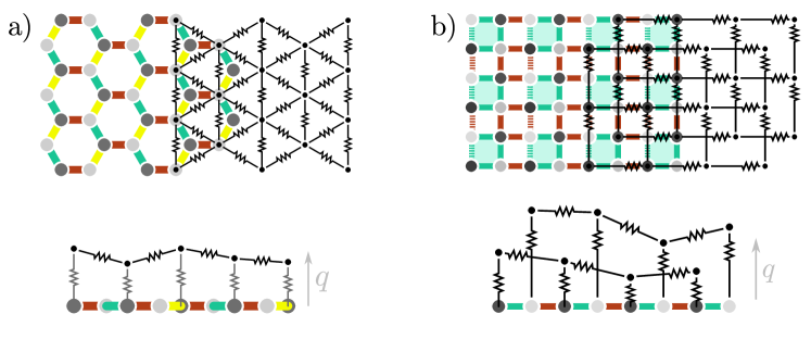
Figure 21: Mechanical analogs of quantum spin liquids. Left: (a) The mechanical Kitaev model is a balls-and-springs model on the triangular lattice, where the masses at each site are restricted to a movement along the axis perpendicular to the lattice plane (see the side view in the lower row). Right: (b) Mechanical analog of a second-order spin liquid on the square lattice.

IV.3 Mechanical analog of the Kitaev spin liquid

The Kitaev spin liquid [106] is a paradigmatic state of matter where spin degrees of freedom fractionalize into itinerant Majorana fermions and a static $\mathbb{Z}_{2}$ gauge structure. On the honeycomb lattice, the Majorana fermions exhibit a gapless Dirac spectrum in the absence of any time-reversal symmetry breaking terms and (roughly) isotropic couplings along the three distinct lattice directions. For strongly anisotropic couplings the Majorana band structure gaps out and one transitions into a topological phase that is primarily defined via its gauge structure as a $\mathbb{Z}_{2}$ toric code. The magic of the Kitaev model is that all these statements have a rigorous analytical foundation. The original spin model with its bond-directional Ising-like exchange terms can be recast in terms of auxiliary Majorana fermion degrees of freedom as a quadratic Majorana Hamiltonian

$${\cal H}_{\rm Kitaev}=\sum_{\langle i,j\rangle_{\alpha}}S_{i}^{\alpha}S_{j}^{\alpha}=-i\gamma^{A}_{i}{\bf A}_{ij}\gamma^{B}_{j}+{\rm h.c.}\,,$$ (59)

that allows for an exact solution [106].

But with an eye on our SUSY correspondence, we note that the right-hand-side of (59) is precisely of the form of the fermionic Hamiltonian (IV.1) used in our SUSY correspondence for real fermions and bosons discussed above. The matrix ${\bf A}$ encodes the hopping of the Majorana fermions described by operators $\gamma^{A}$ and $\gamma^{B}$ on the underlying honeycomb lattice (with the two triangular sublattices $A$ and $B$ as shown in Fig. 21). Following the steps outlined in Section IV.1 above, we can write down its SUSY partner in terms of real bosons, take its classical limit, and arrive at a balls and springs model on the triangular lattice as illustrated in Fig. 21 a) and b). Each mass, located at a site of this triangular lattice, is restricted to a movement along an axis perpendicular to the lattice plane, and is connected via two types of springs to both the plane and its neighboring masses.

This mechanical Kitaev model retains many interesting features of its quantum mechanical counterpart [15]. For instance, its mechanical response exhibits the Dirac spectrum familiar from the quantum model near isotropic coupling – a notable feature for the mechanical system in the sense that on the level of individual springs one always has quadratic excitation spectra and the formation of a linear dispersion constituting the Dirac cone is as such direct evidence of many-body physics. We find that, also in this mechanical model, the Dirac cones have nonzero windings when the supersymmetric Berry phase (53) is computed, with its quantized value $\pm\pi$ solely attributed to the closed-path integral of the SUSY-induced additional term in (52). When moving away from isotropic couplings into the strongly anisotropic toric-code limit of the quantum model, the mechanical analog will again go along and now exhibit a gapped excitation spectrum. This is again a somewhat unusual situation for a mechanical system as the opening of a gap and the absence of any well-defined low-energy modes implies that the mechanical system remains rigid for low-frequency drives – again a many-body phenomenon since individual springs defy any small-frequency rigidity.

Notably such a mechanical Kitaev model not only retains classical analogs of the itinerant Majorana fermions in its propagating phonon modes, it also exhibits its underlying $\mathbb{Z}_{2}$ gauge structure with classical analogs of the static vison excitations of the quantum model. For instance, one can excite a pair of such gauge excitations by switching the sign of an intersite interaction, just like in the quantum case, only that it is a spring constant in the classical context. Individual visons can then be moved around by flipping additional spring constants, e.g., to study braiding in the classical model. One could also set up a scattering experiment where propagating phonon modes and spatially arranged gauge excitations give rise to interference effects, akin to studying the scattering of itinerant Majorana fermions in the presence of massive vison excitations in the quantum model.

IV.4 Mechanical analog of higher-order topological insulator

Being restricted to symmetry class BDI for the Majorana fermion models in our SUSY correspondence of real bosons and fermions, we unfortunately miss one of the more interesting features of the Kitaev honeycomb model – the formation of a gapped topological phase of the Majorana fermions in the presence of time-reversal symmetry breaking (which brings the system into symmetry class D). But despite the absence of such a phase in the classification of topological insulators in symmetry class BDI in two spatial dimensions [21], there is still another possibility for the formation of highly non-trivial band structure – the formation of higher-order topological insulator (HOTI) [122].

Such a HOTI for itinerant Majorana fermions has been discussed in the context of a second-order Kitaev spin liquid [123] where the non-trivial topology manifests itself in gapless Majorana corner modes. While the original spin model in that case has been formulated on the five-coordinated Shastry-Sutherland lattice (in order to retain exact solvability of the spin model), we can here proceed with a somewhat simpler starting point and follow the work of Benalcazar et al. [122] in defining a free Majorana fermion model on the square lattice with staggered couplings among the elementary plaquettes, as illustrated in Fig. 22. Every such elementary plaquette shall be pierced by a $\pi$-flux, so that the Bloch Hamiltonian takes the form

$${\bf H}_{\rm HOTI}({\bf k})=i\begin{pmatrix}&{\bf A}^{\dagger}({\bf k})\\ -{\bf A}({\bf k})&\end{pmatrix},$$ (60)

where

$${\bf A}({\bf k})=\begin{pmatrix}t+\lambda e^{-ik_{x}}&-t-\lambda e^{ik_{y}}\\ t+\lambda e^{-ik_{y}}&\phantom{-}t+\lambda e^{ik_{x}}\end{pmatrix},$$ (61)

with the coupling parameters $t$ and $\lambda$ denoting the interplaquette and intraplaquette hopping strengths, respectively. Feeding this Majorana Hamiltonian into our SUSY correspondence, deriving its real bosonic SUSY partner, and taking its classical limit, we arrive at a balls-and-springs model (Fig. 21) whose onsite and intersite springs have spring constants $t^{2}+\lambda^{2}$ and $-t\lambda$, respectively, and the masses are restricted to move along an out-of-plane axis only.

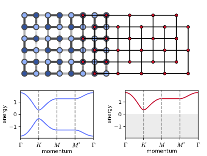
Figure 22: SUSY for a Majorana fermion higher-order topological insulator. Majorana fermions on a decorated square lattice have an isospectral SUSY partner in the form of real bosons on two disjoint copies of the square lattice. Eigenmodes in these systems agree for positive energies.

This mechanical analog of a Majorana HOTI (or the second-order Kitaev spin liquid of Ref. 123) retains, by construction, the gapped spectrum (Fig. 22) and topological response of its quantum mechanical ancestor. Most strikingly, this includes the formation of floppy (gapless) corner modes, which on the mechanical level are tightly interwoven with the onsite spring couplings. The latter are sensitive to the number of neighbors, which in a system with open boundary conditions (i.e., a system with actual edges and corners) gives rise to a spatial variation of these couplings along the boundary of the mechanical system. Notably, a non-Abelian extension of the supersymmetric Berry connection in (52) also enables constructing bosonic Wilson loop operators to decode the topology in this mechanical analog of a HOTI. Such a bosonic topological phase is characterized, like their fermionic counterparts [122], by a quantized quadruple moment that, in this case, follows from the eigenvalues of the bosonic Wilson loops as discussed in detail in Ref. 123. When the coupling parameters of the mechanical model are moved away from the topological trivial regime – where the corner masses experience a restoring force – into the topological regime, these corner masses become essentially free, i.e., they can be moved arbitrarily far from their equilibrium positions without any restoring force. This is the mechanical equivalent of a floppy corner mode and again a testament for many-body physics being at play in this mechanical system.

V Outlook

Our work introduces an application of SUSY to identify free theories of bosons and fermions as superpartners on an extensive variety of lattice geometries that are of high relevance to several condensed matter setups from frustrated magnets to superconductors. At its core, the formulation entails a prescription of squaring and square-rooting Hamiltonians, a mapping that can be elegantly understood in terms of lattice adjacencies in arbitrary spatial dimensions. This mapping then gives rise to topological invariants associated with the single-particle Witten index $\nu$ of the SUSY theory and a five-fold way classification of the SUSY charge.

The mapping from bosons to fermions is a specific highlight for it opens the door to the discovery and/or control of unexpectedly low energy modes in bosonic systems. One could, for example, use this mapping to scan through materials databases seeking topologically protected phonon/magnon zero modes in associated nearest neighbor truncated phonon/magnon models. Next neighbor perturbations would then lift these zero modes to finite energy but leave them at an unexpectedly low energy due to locality. In addition to scanning through a materials database (such as Ref. [124] for topological phonons), one could also use the mapping to design materials with these unexpected low energy modes. In the end, such a program, with an unwanted finite locality replacing the unwanted occupation of bulk modes, is similar to the current search and design of electronic topological materials [125, 126, 127, 128].

A conceptually interesting aspect of the SUSY is that it also allows to establish a connection between the Riemannian structures associated to the manifolds of quantum states (Bloch states) of different lattice models that share identical band structures. Such information is encoded in the quantum geometric tensor [129]

$$\chi_{ij}^{m}=\langle\partial_{k_{i}}u_{m}|(1-|u_{m}\rangle\langle u_{m}|)|\partial_{k_{j}}u_{m}\rangle\,,$$

whose real part yields the quantum metric $g_{ij}$ measuring the distance between nearby quantum states and the imaginary part, the Berry curvature [130]. We observe that, for a number of lattice models connected by SUSY, the imaginary part, i.e. the Berry curvature, appears to be identical for the fermionic and bosonic counterparts, but there is a small, but nonvanishing difference in the associated metric elements $g_{ij}$. This should have immediate impact on physical observables that connect to the quantum metric, which include the anomalous Hall conductivity in a nonuniform electric field [131] or the diamagnetic response of flat band superconductors [132], and should warrant future exploration, particularly exploring these phenomena in SUSY-related bosonic systems.

Another interesting aspect of our SUSY framework is that it also encapsulates theoretical recipes to realize ‘square-root topological phases’ [48, 50, 49, 51] including the $2^{n}$-th root series [52]. In addition, it gives way to envision topological states in bosonic systems by squaring, an approach which, so far, has received limited attention [41], despite the recent proposal [133] that periodically driven systems could unveil new possibilities to realize such exotic phases in the lab. For generic quadratic bosonic systems generated by our SUSY correspondence, a local topology-preserving map can be constructed to reduce them to number-conserving Hamiltonians [134]. To study how SUSY influences such mappings in the space of their fermionic counterparts is an interesting future direction.

While the present work pertains to the non-interacting limit of bosonic and fermionic systems, extending it to interacting systems, such as in the model of (27), could solve a number of interesting puzzles in the field of strongly correlated electrons. It could be that Fendley’s discovery [135] of a SUSY-like mapping between states in the transverse field Ising model/Kitaev chain system may point the way. It is ‘SUSY-like’, because the mapping preserves the states’ energy up to small corrections in the system size. So there is reason to believe that an interacting version of the phenomena discussed in this paper, especially of the Kitaev chain example we discuss, indeed exists. Taking cue from a recently identified strategy for square-rooting the functions of bosonic number operators [136], Heisenberg spin models may also serve as a fertile playground for extending our work to interacting systems. Lastly, if such an interacting version of SUSY exists, it may also provide insights into $\mathbb{Z}_{2}$ quantum spin liquids whose fusion rule $e\times m=\varepsilon$ identifies bosonic spinons paired with $\mathbb{Z}_{2}$ visons as fermionic spinons [137] but are difficult to study beyond exactly solvable models. Perhaps the right step towards solving these puzzles is to connect the SUSY discussed in this manuscript, that requires locality and revealed by lattice geometry, to those discovered to describe certain interacting phase transitions on the surface of certain symmetry protected topological insulators [138, 139, 140].

The most pressing need for such an interacting extension could be to explain the origin of intertwined orders [141] in the cuprates and other high-temperature superconductors. Intertwined orders arise due to a seemingly fine-tuned competition between several ordering tendencies. Physicists working on these systems did not expect accidental degeneracies. They proposed them only after decades of work and surprising discoveries. But such accidental low energy phenomena is a natural consequence of the topology discussed in this paper. While our models exhibit strictly zero-energy modes, actual materials would have soft modes at a finite but low energy, parametrically small in the strength of further neighbor interactions. If someone constructs such a theory, then perhaps it would indeed solidify SUSY as a pillar of condensed matter physics.

Appendix A Graph square-rooting algorithm

The algorithm for taking graph square-roots discussed in this manuscript was first introduced as a “lattice construction” algorithm in Ref. [78]. Here we derive it in a more conceptual manner, starting solely from the fundamental equation of squaring an adjacency matrix,

$$(\mathbf{A}^{2})_{ik}=\sum_{j}\mathbf{A}_{ij}\mathbf{A}_{jk}\,.$$ (62)

It is apparent that an edge between vertices $i$ and $k$ in the squared graph corresponds to (the sum of all) combinations of edges going from vertex $i$ to $k$ via intermediate vertices $j$. In more practical terms, this constitutes the next-nearest neighbors of the graph.

It is well known that in a bipartite graph, the next-nearest neighbors of one of the two sublattices only reside within that sublattice. Therefore, if one would construct a bipartite graph for a given lattice in such a way that the given lattice arises from taking next-nearest neighbors in the bipartite graph, one would naturally define a second sublattice which can be viewed as the superpartner to the given lattice.

The last piece of the algorithm is to show how exactly one can define a bipartite graph in such a way for a given lattice. This construction is at the heart of the lattice construction algorithm and relies on the observation that locally, a $z$-coordinated site of one sublattice in the bipartite graph results in a fully-connected plaquette (or clique in graph language) with $z$ vertices in the other sublattice upon squaring. c.f. Fig. 2. Therefore, to go the other way, we propose to replace all $z$ cliques by $z$-coordinated sites, constituting the new sublattice and thus producing the bipartite graph.

For practical applications, note that every $z$ clique contains cliques of order $z-1$. One therefore needs to mandate that the algorithm should start by replacing maximal plaquettes in descending order of their size. This will guarantee that one replaces a minimal amount of plaquettes. It is further known from computer science that finding all maximal cliques in a graph is generally an NP-hard problem. However, in a physics situation the graphs one usually has to deal with are lattices whose unit cells have a rather finite number of elements which in turn puts an upper limit on how large cliques can become and thereby greatly alleviates the problem of clique identification.

Note also, that the replacement of plaquettes can only guarantee the connectivity of the graph, but not its labels. In a physical situation, hopping (or interaction) strengths would appear as labels in the adjacency matrix, which further complicates the calculation of the labels within the bipartite graph. However, in all cases (62) should be fulfilled.

In total, the entire lattice construction algorithm can be summarized as follows, assuming one is given a lattice with labels and connectivity:

1. Identify all cliques within the lattice.

2. In descending order, do the following to every clique:

   1. Add a new vertex in the center of the clique.

   2. Add edges between this new vertex and the other vertices of the clique.

   3. Remove vertices of the clique.

3. Here, all the old edges of the initial lattice should have been removed and only the newly added edges connecting the old and new vertices are retained in the lattice.

4. Assign labels to the newly added edges; reduce the number of labels using graph symmetries.

5. Use (62) to produce a system of equations which link the newly created labels to the old labels.

6. Solve these equations to obtain fitting labels for the bipartite lattice.

7. To obtain the second sublattice, being the SUSY partner of the given lattice, construct next-nearest neighbors and use (62) to correctly label the edges.

In summary, this algorithm provides a method to generate a partner lattice of a given lattice. Note that especially step 4. includes optional and ambiguous instructions which may depend greatly on the situation specified. Therefore, the algorithm does not deliver a unique solution but only one that is compliant with graph-rules and squaring.

Connection to other lattice correspondences

Let us connect our graph squaring and square-rooting algorithm to other approaches of establishing lattice correspondences in the literature:

• The first such approach pairs medial and pre-medial lattices to one another – examples include, for instance: the honeycomb is the premedial lattice of the kagome (and the kagome the medial lattice of the honeycomb), the hyperoctagon is the premedial of the hyperkagome, and the diamond is the premedial lattice of the pyrochlore.

  All of these lattice correspondences are captured by our SUSY graph correspondence and the graph square-rooting algorithm above. According to this algorithm, the SUSY partner for a given lattice will be the pre-medial lattice if all graph cliques are of the same size, i.e. there is only a single type of maximally connected plaquettes (triangles in the case of kagome and hyperkagome, tetrahedra in the case of the pyrochlore). In such cases, the SUSY partner will also feature an equal coordination number on all sites, which goes hand in hand with having a single type of cliques on the original lattice.

• Another special case is the formulation of a line-graph for a given lattice geometry which one obtains from connecting the vertices on the center of all bonds – examples again include the kagome lattice, which is the line-graph of the honeycomb lattice, or the 3D Shastry-Sutherland lattice which is the line-graph of the hyperoctagon lattice (see Fig. 17).

  This correspondence is again captured by our graph square-rooting algorithm when applied to a scenario where the biggest (and only) type of clique in a graph is simply a single two-site bond.

• A third connection can be made to the formulation of a Lieb lattice [144]. The latter most often refers to the lattice that we have denoted as square-X lattice (see Fig. 24) – a square lattice where one adds an additional site to each bond of the lattice. This bipartite lattice decomposes into two sublattices, the original square lattice and its line-graph, the checkerboard lattice.

  As such the Lieb lattice is most naturally identified with the SUSY charge lattice of our lattice correspondence, i.e. the superposition of the two SUSY partnering lattice geometries identified by our graph square-rooting algorithm. This also allows to readily generalize the concept of the Lieb lattice to all lattice geometries considered in the triptych-like figures of Section III, for instance, the honeycomb-X lattice as Lieb lattice of the honeycomb lattice or the hyperhoneycomb-X lattice as the Lieb lattice of the hyperhoneycomb lattice and so on.

It should be noted that while these others lattice correspondences have not been explicitly discussed as SUSY correspondences, some authors have used these to construct flat-band models, i.e. models with a non-zero Witten index, such as in the context of line-graphs [145, 146, 147] or Lieb lattices [144]. For a pedagogical overview see Refs. 148 and 149.

Appendix B Five-fold way classification of SUSY models

In this Appendix, we will present a detailed discussion of the symmetry-based classification of Hermitian supercharges. A key result of this approach is that, by imposing the conventional symmetries that classify the Hamiltonians of free fermionic systems [37, 38, 39, 40], the supercharge can belong to one of the five distinct classifying spaces, which leads us to a five-fold way classification as will be elaborated in the following.

A supercharge is fundamentally characterized by the Witten index $\nu$: its Bloch spectrum features precisely $\nu$ flat bands at zero energy. The topology of additional band-degeneracy points at zero energy coinciding with the flat bands, so-called nexus points [56, 57, 58, 59], has a remarkable dependence on this Witten index $\nu$ that can be understood in terms of homotopy maps [43]. Of specific interest in the parlance of condensed matter setups are: (i) the zeorth homotopy group $\pi_{0}({\cal M})$, which is the set of mappings of a single point into a classifying (or topological) space $\cal M$ and can lead to topological invariants like sign[Pfaffian] (the emergence of such an invariant has been discussed in, e.g., Refs. [150] and [35]), (ii) the first or the fundamental homotopy group $\pi_{1}({\cal M})$, which is the set of mappings of loops into $\cal M$ and gives rise to invariants such as the Berry phase, (iii) the second homotopy group $\pi_{2}({\cal M})$, the set of mappings of closed surfaces into $\cal M$ leading to invariants like the Chern number, and (iv) the third homotopy group $\pi_{3}({\cal M})$, the set of mappings of closed volumes into $\cal M$ characterizing, e.g., Hopf insulators [151]. In what follows, we will elucidate the five-fold classification of supercharges for each value of $\nu$ and specializing to homotopy groups $\pi_{n}$ from $n=0$ to $3$. In a subsequent Appendix, Appendix C, we will provide a number of examples by classifying the topology of some of the lattice models in two and three dimensions that are discussed in the main text.

Let us start our discussion by considering the matrix representing the Hermitian supercharge ${\cal Q}_{\rm H}$ in (II.4), which, by the very nature of our SUSY construction, is chiral, i.e., it takes the general form

$${\bf H}=\begin{pmatrix}&{\bf R}\\ {\bf R}^{\dagger}&\end{pmatrix}\,.$$ (63)

Symmetry-wise it therefore belongs to one of the five chiral classes AIII, BDI, CII, CI, or DIII in the ten-fold way classification [39]. Table 2 summarizes how the time-reversal ${\cal T}$ and the particle-hole ${\cal P}$ operator behave in each one of these classes (while all have the chiral symmetry, i.e., ${\cal C}^{2}=1$) and the resultant classifying spaces ($\cal M$) of the (spectrally-flattened) Hamiltonians [38].

Cartan label	${\cal T}^{2}$	${\cal P}^{2}$	${\cal C}^{2}$	Classifying space
AIII	0	0	1	$U(N)$
BDI	1	1	1	$O(N)$
CII	-1	-1	1	$Sp(2N)$
CI	1	-1	1	$U(N)/O(N)$
DIII	-1	1	1	$U(2N)/Sp(2N)$

Table 2: Five chiral symmetry classes which a chiral Hamiltonian can belong to. The last column is of the corresponding classifying spaces of the K-theory [38].

The antiunitary symmetry operators, ${\cal T}$ and ${\cal P}$, and the unitary symmetry operator ${\cal C}$ in each one of these classes impose specific conditions on the matrix ${\bf H}$ when we consider it as a first-quantized Hamiltonian, namely,

$${\cal T}{\bf H}{\cal T}^{-1}={\bf H}\leavevmode\nobreak\ ;\leavevmode\nobreak\ {\cal P}{\bf H}{\cal P}^{-1}=-{\bf H}\leavevmode\nobreak\ ;\leavevmode\nobreak\ {\cal C}{\bf H}{\cal C}^{\dagger}=-{\bf H}\,.$$ (64)

Adapting a canonical representation of these symmetries in each of the five classes of Table 2, one can understand what these conditions have to imply for the matrix ${\bf R}$ which we list in Table 3.

Cartan	${\cal T}$	${\cal P}$	${\cal C}$	condition on $\bf R$
label
AIII	—	—	$\sigma_{3}$	—
BDI	${\cal K}$	$\sigma_{z}{\cal K}$	$\sigma_{3}$	$\bf R^{*}={\bf R}$
CII	$\sigma_{3}\otimes i\sigma_{2}{\cal K}$	$-1\otimes i\sigma_{2}{\cal K}$	$\sigma_{3}\otimes 1$	$(i\sigma_{2}){\bf R}^{*}(-i\sigma_{2})={\bf R}$
CI	$\sigma_{1}{\cal K}$	$-i\sigma_{2}{\cal K}$	$\sigma_{3}$	$\bf R^{T}={\bf R}$
DIII	$i\sigma_{2}{\cal K}$	$\sigma_{1}{\cal K}$	$\sigma_{3}$	$\bf R^{T}=-{\bf R}$

Table 3: Canonical representation of the symmetries in the five chiral classes. $\cal K$ denotes complex conjugation. The last column enlists the condition to be obeyed by the matrix ${\bf R}$ in each of these classes in compliance with (64).

Let us now remind us of the fact that SUSY renders a Witten index $\nu$ to each ${\bf R}$ in terms of its dimensions: for ${\bf R}$ being an arbitrary $M\times N$ matrix, $\nu=N-M$. Therefore, when ${\bf R}$ is a square matrix, which is referred to as the isostatic case, the Witten index is $\nu=0$ whereas for a rectangular $\bf R$ matrix, the nonisostatic cases, $\nu\neq 0$, the latter exclusively manifesting in flat bands in conjunction with (degenerate) point nodes in the band structures of $\bf H$.

For the flat bands in a SUSY problem always appear at zero energy, their topology cannot be chassified in terms of the ten-fold way. In fact, for the first three classes – AIII, BDI, and CII – the different values of $\nu$ (the isostatic and the nonisostatic cases) exhibit distinct topology as discussed by two of us [43] in terms of homotopy groups $\pi_{n}$ (mapping the $n$-dimensional sphere ${\cal S}_{n}$ to the classifiying spaces ${\cal M}$ in Table 2. For the last two classes – CI and DIII – ${\bf R}$ must be a square matrix and one can as well compute the stable homotopy groups of the respective classifying spaces (following Bott’s original work [152]), which will be independent of $\nu$. This leads us to the aforementioned five-fold way classification of the supersymmetric lattice models, i.e., the supercharges, which is shown in Table 4, where we list the possible topological invariants, for each of the five symmetry classes, as a function of Witten index and the homotopy groups up to $\pi_{3}$, relevant for models in $d=1,2,3$ dimensions. For the reader’s convenience, we also reorganize the results from this table for specific Witten indices in Tables 5 ($\nu=0$) and 6 ($\nu=1$).

Cartan label	$\quad\nu\quad$	$\quad\pi_{0}\quad$	$\quad\pi_{1}\quad$	$\quad\pi_{2}\quad$	$\quad\pi_{3}\quad$
AIII	0	0	$\mathbb{Z}$	0	$\mathbb{Z}$
	1	0	0	$\mathbb{Z}$	0
	$\geq$ 2	0	0	0	0
BDI	0	$\mathbb{Z}_{2}$	$\mathbb{Z}_{2}$	0	$\mathbb{Z}$
	1	0	$\mathbb{Z}_{2}$	0	$\mathbb{Z}$
	2	0	0	$\mathbb{Z}$	$\mathbb{Z}$
	3	0	0	0	$\mathbb{Z}$
	$\geq$ 4	0	0	0	0
CII	0	0	0	0	$\mathbb{Z}$
	$\geq$ 1	0	0	0	0
CI	0	0	$\mathbb{Z}$	$\mathbb{Z}_{2}$	$\mathbb{Z}_{2}$
	$\geq$ 1	0	$\mathbb{Z}$	$\mathbb{Z}_{2}$	$\mathbb{Z}_{2}$
DIII	0	0	$\mathbb{Z}$	0	0
	$\geq$ 1	0	$\mathbb{Z}$	0	0

Table 4: Five-fold way classification table of SUSY lattice models (the supercharges). For each of the five chiral symmetry classes, the table indicates topological invariants ($\mathbb{Z}_{2}$, $\mathbb{Z}$) as a function of Witten index $\nu$ and homotopy groups $\pi_{n}$. It thereby generalizes Table 1 of the main text, which is specific to symmetry class BDI. For symmetry classes AIII, BDI, and CII, Witten indices $\nu$ greater than the listed values exhibit trivial topology, while for the class CI and DIII, the topology turns out to be the same for any $\nu\neq 0$ and $\nu=0$. For the reader’s convenience, we have also resorted the results from this Table for fixed Witten indices in Tables 5 ($\nu=0$) and 6 ($\nu=1$).

Note in the above discussion, the Witten index $\nu$ is of fundamental importance and not the spatial dimensionality of a model unlike what is typically done in the ten-fold way classification tables to reveal strong invariants [37, 38, 39, 40]. When computing a topological invariant of a lattice model, we often resort to the band structures in $d$ dimensions, characterized by the pseudomomenta ${\bf k}$, for which a $d$-dimensional torus $\mathbb{T}_{d}$ should be considered as the base manifold instead of the sphere ${\cal S}_{d}$. But in doing so, it turns out we only miss out the information about weak topological invariants (which can exist only in translation symmetric systems). To note, in presence of such a parameter $\bf k$, the conditions noted in Table 3 become

$${\rm BDI:}\leavevmode\nobreak\ \leavevmode\nobreak\ \bf R^{*}({\bf k})={\bf R}(-{\bf k})\,,$$

$${\rm CII:}\leavevmode\nobreak\ \leavevmode\nobreak\ \leavevmode\nobreak\ (i\sigma_{2}){\bf R}^{*}({\bf k})(-i\sigma_{2})={\bf R}(-{\bf k})\,,$$

$${\rm CI:}\leavevmode\nobreak\ \leavevmode\nobreak\ \leavevmode\nobreak\ \leavevmode\nobreak\ \bf R^{T}({\bf k})={\bf R}(-{\bf k})\,,$$

$${\rm DIII:}\leavevmode\nobreak\ \leavevmode\nobreak\ \bf R^{T}({\bf k})=-{\bf R}(-{\bf k})\,.$$ (65)

Here we seek to explore the topology of the nodes in the band structures of $\bf H$ at zero energy that involve flat bands. The relevant parameter is what is known as the node dimensionality, which is distinct from the spatial dimensionality. The node dimensionality turns out to be dictated primarily by the Witten index. For a characterization of such nodes in the ten Atland-Zirnbauer (AZ) classes without the flat bands (i.e., the isostatic case, $\nu=0$) in terms of homotopy groups, we refer to Ref. [150] where this has previsouly been established. The present work generalizes these ideas to non-zero Witten index $\nu\neq 0$ for the five chiral AZ classes.

Cartan label	$\nu=0$
	$\quad\pi_{0}\quad$	$\quad\pi_{1}\quad$	$\quad\pi_{2}\quad$	$\quad\pi_{3}\quad$
AIII	0	$\mathbb{Z}$	0	$\mathbb{Z}$
BDI	$\mathbb{Z}_{2}$	$\mathbb{Z}_{2}$	0	$\mathbb{Z}$
CII	0	0	0	$\mathbb{Z}$
CI	0	$\mathbb{Z}$	$\mathbb{Z}_{2}$	$\mathbb{Z}_{2}$
DIII	0	$\mathbb{Z}$	0	0

Table 5: Five-fold classification table of SUSY lattice models (the supercharges) for fixed Witten index $\nu=0$ providing the topological invariants for each symmetry class and the first four homotopy groups $\pi_{n}$.

Cartan label	$\nu=1$
	$\quad\pi_{0}\quad$	$\quad\pi_{1}\quad$	$\quad\pi_{2}\quad$	$\quad\pi_{3}\quad$
AIII	0	0	$\mathbb{Z}$	0
BDI	0	$\mathbb{Z}_{2}$	0	$\mathbb{Z}$
CII	0	0	0	0
CI	0	$\mathbb{Z}$	$\mathbb{Z}_{2}$	$\mathbb{Z}_{2}$
DIII	0	$\mathbb{Z}$	0	0

Table 6: Five-fold classification table of SUSY lattice models (the supercharges) for fixed Witten index $\nu=1$ providing the topological invariants for each symmetry class and the first four homotopy groups $\pi_{n}$.

The following Appendix will illuminate the topology of several lattice models all of which have a chiral Bloch Hamiltonian as in (63) representing their Hermitian supercharge ${\cal Q}_{\rm H}$. All these examples belong to symmetry class BDI. We seek to find appropriate topological invariants that fit the BDI class in Table 4 by computing the relevant $\pi_{n}$ for a given Witten index $\nu$.

Appendix C Topology of the SUSY lattice models in BDI class

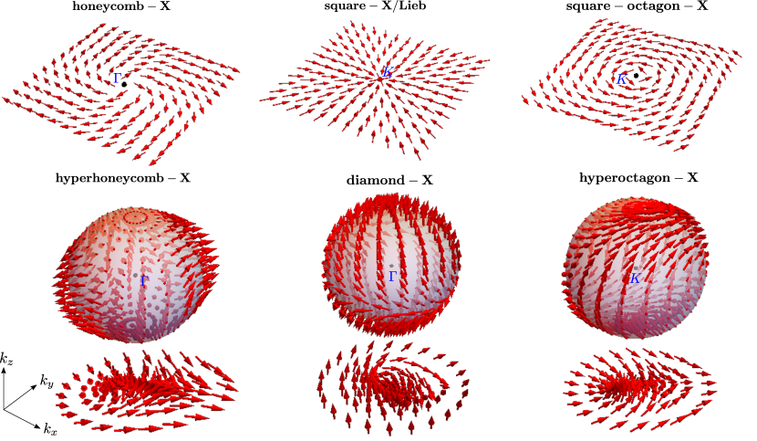
Figure 23: Topological invariants from homotopy. The three examples for two-dimensional lattice geometries in the top row exhibit a non-trivial homotopy associated with $\pi_{1}$, i.e., a non-trivial Berry phase around the nexus points located at high-symmetry points in the Brillouin zone (indicated in blue). Shown are the SUSY charge lattices honeycomb-X (Fig. 1), square-X/Lieb lattice (Fig. 24), and square-octagon-X (Fig. 7). The three examples for three-dimensional lattice geometries in the bottom row, exhibit a non-trivial homotopy for $\pi_{2}$ (and are hence plotted over a unit sphere ${\cal S}_{2}$ and its projection onto $\mathbb{R}^{2}$), i.e., they exhibit a non-trivial skyrmion number when projecting onto the two-dimensional plane (bottom row). Shown are the SUSY charge lattices hyperhoneycomb-X (Fig. 8), diamond-X (Fig. 16), and hyperoctagon-X (Fig. 17). The topology in these examples follows from the homotopy classification of the BDI class against the Witten index $\nu$ as shown in Table 1. For all examples plotted are the different components of the vector ${\bf d}({\bf k})$ that represents an effective Bloch Hamiltonian linearized around the band degeneracy points at zero energy [see (66)].

In order to appreciate the topology of the SUSY models (the supercharges) with non-zero Witten index $\nu\neq 0$, which we have classified in the previous Appendix, we return to some of the principal examples from the main text (illustrated in the triptych-like figures of Section III) and elucidate the non-trivial topological invariants with the nexus points of their respective supercharge models. The latter arise from nontrivial homotopy groups $\pi_{1}$ and $\pi_{2}$ in two- and three-dimensional lattice geometries, respectively. Note that all examples are in symmetry class BDI.

We will focus on the part of the band structures near the band degeneracy points at zero energy that include the flat bands and might exhibit additional band degeneracies, e.g., in the form of Dirac crossings, at the so-called nexus points. The basic idea now is to project onto the relevant bands of the original chiral Bloch Hamiltonian ${\bf H}(\bf k)$ near such a band-degeneracy point and derive an effective Hamiltonian $\tilde{\bf H}(\bf k)$ involving only those bands. This effective Hamiltonian $\tilde{\bf H}(\bf k)$ is not generally in a chiral form but we can adopt a basis in which the chiral symmetry operator is diagonal and re-express $\tilde{\bf H}(\bf k)$ in that basis to restore its chiral form. Depending on its dimension $N$, $\tilde{\bf H}(\bf k)$ can be written in terms of the suitable SU$(N)$ generators ${\bf\Lambda}$ as

$$\tilde{\bf H}(\bf k)={\tilde{\bf H}}_{0}+{\bf d}({\bf k})\cdot\Lambda\,,$$ (66)

where ${\tilde{\bf H}}_{0}$ is the effective Hamiltonian at the degeneracy point. We will then inspect the profile of the vector ${\bf d}({\bf k})$ in the Fourier space (as illustrated in Fig. 23 above) over loops or spheres encompassing the degeneracy point depending on the Witten index $\nu$ of the supercharge to begin with.

Let us illustrate this procedure with examples for some of the lattice models with $\nu\neq 0$ studied in this manuscript in the following:

Honeycomb-X lattice (Fig. 1): For the honeycomb-kagome SUSY correspondence, the Hermitian superhcarge yields a Bloch Hamiltonian on the intermediate honeycomb-X lattice that has a flat band and a three-fold degeneracy at the $\Gamma$-point of the Brillouin zone. With a Witten index of $\nu=1$ in this case ${\bf R}({\bf k})$ is a $2\times 3$ matrix. Around the $\Gamma$-point, we obtain a $3\times 3$ effective Hamiltonian $\tilde{\bf H}(\bf k)$ which we linearize to obtain the vector ${\bf d}(\bf k)$. This vector turns out to have two components which, when plotted over the Brillouin zone, reveals a full winding over any closed path around the $\Gamma$-point (see Fig. 23). We are therefore able to conclude that this model exhibits nontrivial topology, just as Table 4 suggests for $\pi_{1}$ with $\nu=1$. As long as the degeneracy involving the flat band is indeed present, we find perturbations cannot destroy such winding pattern rendering it a topological nature.

Square-X / Lieb lattice (Fig. 24): For the square-X (Lieb) lattice, we have a Witten index of $\nu=1$ and ${\bf R}({\bf k})$ is a $1\times 2$ matrix. The original Block Hamiltonian ${\bf H}({\bf k})$ is $3\times 3$ matrix, and no further projection is required. The band structure has a three-fold degeneracy at $K=(\pm\pi,\pm\pi)$. The winding of the resultant two-component ${\bf d}({\bf k})$ vector, obtained by linearizing ${\bf H}({\bf k})$ around one of the $K$-points, is shown in Fig. 23 revealing a nontrivial topology due to $\pi_{1}$.

Square-octagon-X lattice (Fig. 7): The square-octagon-X lattice mediates the SUSY correspondence between the square-octagon and the squagome lattice. This is an example with Witten index $\nu=2$ and an ${\bf R(k)}$ of dimensions $4\times 6$. A four-fold degenerate point is present along with two flat bands at the four corners of the Brillouin zone with $K=(\pm\pi/(2+\sqrt{2}),0)$ and $K^{\prime}=(0,\pm\pi/(2+\sqrt{2}))$. Adapting a basis in which the chiral symmetry is diagonal, we find the effective $4\times 4$ Hamiltonian to take a chiral form with an effective $1\times 3$ $\tilde{\bf R}$-matrix. However, after linearizing around one of the $K$-points at play, we find the vector ${\bf d}({\bf k})$ is two-component only. The winding of this vector around the $K$-point is shown in Fig. 23, for which we need to immediately express a word of caution: while the plot might seem to suggest that there is a nontrivial topology associated with $\pi_{1}$ for this $\nu=2$ model (and a trivial topology for $\pi_{2}$), this is unexpected for BDI class at $\nu=2$, see Table 1. One possible explanation is the existence of another symmetry that changes the class, but we have not investigated this issue further.

In a similar fashion to the two-dimensional examples discussed above, we can now move on to analyze some three-dimensional SUSY models:

Diamond-X lattice (Fig. 16): The Hermitian supercharge responsible for the SUSY correspondence between the diamond and pyrochlore lattices can be envisaged as a chiral Bloch Hamiltonian on the intermediate diamond-X lattice. This is another example for a Witten index $\nu=2$ and an ${\bf R}({\bf k})$ of dimensions $2\times 4$ (akin to the square-octagon-X lattice discussed above). A four-fold degenerate point is present along with two flat bands at the $\Gamma$-point of the Brillouin zone. After linearizing the effective Hamiltonian, which is a $4\times 4$ chiral matrix with an off-diagonal block $\tilde{\bf R}({\bf k})$ of dimensions $1\times 3$, around the $\Gamma$-point, we find the vector ${\bf d}({\bf k})$ is of three components. Plotted over the Brillouin zone (see Fig. 23), it reveals a hedgehog texture surrounding the $\Gamma$-point arising from a nontrivial topology due to $\pi_{2}$ as Table 4 suggests. Projecting this texture onto two spatial dimensions reveals a skyrmion, a whirl in the texture which is another manifestation of the non-trivial topology at play here.

Hyperhoneycomb-X lattice (Fig. 8): The Hermitian charge mediating the SUSY correspondence between the hyperhoneycomb lattice and its SUSY partner is a Bloch Hamiltonian on the hyperhoneycomb-X lattice. This is a $\nu=2$ system with a fourfold degeneracy at the $\Gamma$-point of the Brillouin zone and two flat bands. After linearizing, the effective Hamiltonian takes the form a $4\times 4$ chiral matrix with an off-diagonal block $\tilde{\bf R}({\bf k})$ of dimensions $1\times 3$, around the $\Gamma$-point. We find the vector ${\bf d}({\bf k})$ is of three components. When plotted over the Brillouin zone (see Fig. 23), it reveals a hedgehog texture surrounding the $\Gamma$-point (and a two-dimensional skyrmionic projection) arising from a nontrivial topology due to $\pi_{2}$ as Table 4 suggests.

Hyperoctagon-X lattice (Fig. 17): The Hermitian charge mediating the SUSY correspondence between the hyperoctagon lattice and its SUSY partner, the hyperkagome lattice, manifests as a Bloch Hamiltonian on the hyperoctagon-X lattice. This is yet another $\nu=2$ system with fourfold degeneracy at the $K$-point of the Brillouin zone and two flat bands. After linearizing around the $K$-point, the effective Hamiltonian takes the form a $4\times 4$ chiral matrix with an off-diagonal block $\tilde{\bf R}({\bf k})$ of dimensions $1\times 3$. We find the vector ${\bf d}({\bf k})$ is of three components. Plotted over the Brillouin zone (see Fig. 23), it reveals a hedgehog texture surrounding the $K$-point (and a two-dimensional skyrmionic projection) arising from a nontrivial topology due to $\pi_{2}$ as indicated by Table 4.

Appendix D Additional examples of SUSY lattice correspondences

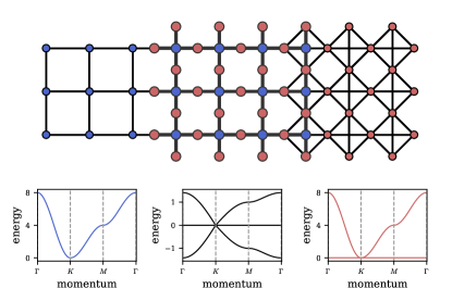
Figure 24: SUSY corresponding square and checkerboard lattices. Complex fermions (blue, left) on the square lattice are supersymmetrically linked to complex bosons (red, right) on the checkerboard lattice. The mapping can be established with a SUSY charge which can be interpreted as the adjacency matrix of a square-X lattice (center plot), i.e., a square lattice with additional sites on every bond whose two sublattices are the square and checkerboard lattices respectively. For the topological classification according to Table 1, we find, noting that the Witten index here is $\nu=1$, that the nexus point in the SUSY charge spectrum has a trivial topological invariant of $\pi_{1}=+1$, see also the illustration in Fig. 23 of the Appendix.

In addition to the SUSY lattice correspondences for tight-binding models of complex fermions and bosons presented in the main manuscript we provide two more instances here. The first example is a SUSY lattice correspondence between the square lattice and the checkerboard lattice (which is sometimes also referred to as planar pyrochlore lattice) via the square-X lattice (Fig. 24) that is commonly referred to as the Lieb lattice [144]. The additional site in the checkerboard unit cell with regard to the square lattice manifests itself in a single flat band in the checkerboard band structure, pointing to an extensive ground-state manifold of the Heisenberg antiferromagnet on this lattice [34].

The second example (Fig. 25) pertains to the square-octagon lattice whose two sublattices each constitute a so-called Shastry-Sutherland lattice [153], which has been extensively discussed in the context of SrCu₂(BO₃)₂ [154, 155, 156]. This SUSY lattice correspondence allows to formulate a spin-fermion SUSY correspondence between the spin physics on the Shastry-Sutherland lattice and fermions on the square-octagon lattice, the planar variant of the three-dimensional scenario that we discussed in the main text when connecting the hyperoctagon lattice and a 3D generalization of the Shastry-Sutherland lattice (Fig. 14).

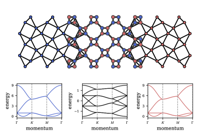
Figure 25: SUSY corresponding Shastry-Sutherland lattices. Complex fermions (blue, left) on Shastry-Sutherland lattice are supersymmetrically linked to complex bosons (red, right) on the same lattice. The mapping can be established with a SUSY charge which can be interpreted as the adjacency matrix of a square-octagon lattice (center plot) whose two sublattices are both Shastry-Sutherland lattices. For the topological classification according to Table 5, we find, noting that the Witten index here is $\nu=0$, that the Fermi surface in the SUSY charge spectrum has a trivial topological invariant of $\pi_{1}=0$.

We can employ the same lattice correspondence also to construct an interesting mechanical model. To do so, we would employ the SUSY correspondence for real bosons and fermions of Section IV.1 and connect Majorana fermions on the square-octagon lattice, the relevant description of the square-octagon Kitaev model [157], to a spring-mass network forming the Shastry-Sutherland lattice. Importantly, the mechanical model allows us to also vary the flux sectors of this model thereby probing both gapped and gapless Majorana spectra in the $\pi$-flux and zero-flux phases, respectively.

In detail, the Majorana Hamiltonian on the square-octagon lattice is defined as

$${\bf H}_{F}({\bf k})=i\begin{pmatrix}&-{\bf A}^{\dagger}({\bf k})\\ {\bf A}({\bf k})&\end{pmatrix},$$ (67)

with

$${\bf A}({\bf k})=$$

$$t\begin{bmatrix}1/z_{x}&1/z_{y}&(z_{x}z_{y})^{1/\sqrt{2}}&0\\ z_{y}&z_{x}&0&(z_{x}z_{y})^{-1/\sqrt{2}}\\ 0&(z_{y}/z_{x})^{1/\sqrt{2}}&1/z_{y}&z_{x}\\ (z_{x}/z_{y})^{1/\sqrt{2}}&0&1/z_{x}&z_{y}\end{bmatrix},$$ (68)

where $z_{x,y}\equiv e^{ik_{x,y}}$ and $t$ denotes the hopping strengths. The unit cell here comprises eight sites included in a basis $\begin{pmatrix}\gamma^{A}_{1{\bf k}}&\gamma^{A}_{2{\bf k}}&\gamma^{A}_{3{\bf k}}&\gamma^{A}_{4{\bf k}}&\gamma^{B}_{1{\bf k}}&\gamma^{B}_{2{\bf k}}&\gamma^{B}_{3{\bf k}}&\gamma^{B}_{4{\bf k}}\end{pmatrix}^{T}$.

This fermionic Hamiltonian can be generated by a supercharge whose matrix form is

$${\bf R}({\bf k})=\begin{pmatrix}{\bf 1}&\\ &{\bf A}({\bf k})\end{pmatrix}.$$ (69)

The bosonic model it yields is defined on the Shastry-Sutherland lattice with the sites hosting unit masses and the bonds the springs including intrasite contributions as the other examples. This is an intriguing case of a mechanical setup where the phonon spectrum exhibits a manifold of Goldstone modes that form a line in momentum space (akin to a Fermi surface). Note that the spectrum also exhibits a flat band section along a path between certain high-symmetry points ($\Gamma$ to $K$) in the Brillouin zone.

Appendix E Topology for complex fermion-boson SUSY correspondence

Topological twists (or defects) in fermionic bands can be characterized by quantized phases or integer-valued invariants originating from the homotopy classification of tight-binding Hamiltonians [158, 159, 39]. For instance, the Berry phase has been an incredibly useful tool to characterize the topology of (nodal) band structures in electronic systems [160, 161, 162, 163].

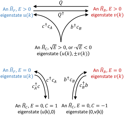
Figure 26: An eigenstate “olog” of SUSY states [164] showing the mappings of single particle eigenstates between the chiral fermion model ${\cal H}_{C}$ associated with the SUSY charge [see Eq. (II.4)], the boson model ${\cal H}_{B}$ and the fermion model ${\cal H}_{F}$ [see Eq. (II.1)]. Notice the zero energy space of ${\cal H}_{C}$ splits into two sectors, one on the $A$ sublattice that maps to eigenstates of ${\cal H}_{F}$ and one on the $B$ sublattice that maps to eigenstates of ${\cal H}_{B}$. Following a given eigenstate of ${\cal H}_{C}$ with finite energy leads to the same state independent of which path is taken. Note: the mapping under $Q$, $Q^{\dagger}$ of the many-body ${\cal H}_{\rm SUSY}$ states, follows a similar pattern, with $Q$, preserving $R=N_{F}+N_{B}$, the so-called “$R$” symmetry [165], mapping the eigenstates in Fock sector $(N_{F},N_{B})$ to those in Fock sector $(N_{F}+1,N_{B}-1)$ and $Q^{\dagger}$ mapping $(N_{F},N_{B})$ to $(N_{F}-1,N_{B}+1)$.

Berry Phases. For the SUSY lattice models at hand, specified via the Hamiltonians ${\bf RR^{\dagger}}$ and ${\bf R^{\dagger}R}$, the Berry phases associated with the corresponding Bloch wavefunctions turn out to be intimately related. Using the wavefunction relations of Eq. (13), illustrated in Fig. 26, one can show that if the closed-orbit Berry phase for a (fermionic) eigenfunction of ${\bf RR^{\dagger}}$ is given by

$$\theta_{F}^{{\bf RR^{\dagger}}} =i\oint\langle u({\bf k})|\partial_{\bf k}u({\bf k})\rangle\cdot{\rm d}{\bf k}\,,$$ (70)

then the one for the (bosonic) eigenfunction of ${\bf R^{\dagger}R}$ at the same energy will be

$$\theta_{B}^{{\bf R^{\dagger}R}} =i\oint\langle v({\bf k})|\partial_{\bf k}v({\bf k})\rangle\cdot{\rm d}{\bf k}$$ (71)

$$=\theta_{F}^{{\bf RR^{\dagger}}}-\oint\frac{{\operatorname{Im}}(\langle u({\bf k})|(\partial_{\bf k}{\bf R})|v({\bf k})\rangle)}{\sqrt{\omega_{n}({\bf k})}}\cdot{\rm d}{\bf k}\,.$$

Of particular interest here is the additional term in the second line, which points to a potential difference in the bosonic and fermionic Berry phases. It is a direct consequence of the wavefunction correspondence in (13) and notably involves both the fermionic and bosonic states. If we reexpress it entirely in terms of the bosonic states by further utilizing the mapping in (13), we arrive at a SUSY version of the bosonic Berry phase

$$\theta_{B}^{\rm SUSY} =i\oint\langle v({\bf k})|\partial_{\bf k}v({\bf k})\rangle\cdot{\rm d}{\bf k}$$

$$\leavevmode\nobreak\ \leavevmode\nobreak\ \leavevmode\nobreak\ \leavevmode\nobreak\ \leavevmode\nobreak\ \leavevmode\nobreak\ +\oint\frac{{\operatorname{Im}}(\langle v({\bf k})|{\bf R}^{\dagger}(\partial_{\bf k}{\bf R})|v({\bf k})\rangle)}{\omega_{n}({\bf k})}\cdot{\rm d}{\bf k}\,.$$ (72)

Only if the integrand in the second augmenting term can be written as $\partial_{\bf k}{\cal F}({\bf k})$ for some function ${\cal F}({\bf k})$, then the conventional Berry phases $\theta_{F}$ and $\theta_{B}$, acquired under adiabatic evolution along any closed orbit, in the two supersymmetrically related systems will be equal. Such a vanishing of the augmenting term would also be ensured by imposing that the matrix ${\bf R}^{\dagger}(\partial_{\bf k}{\bf R})$ at its heart is Hermitian and $[{\bf R}^{\dagger},\partial_{\bf k}{\bf R}]=0$. (For a Hermitian ${\bf R}$ these two conditions are in fact equivalent ). For the honeycomb-kagome correspondence described above, where both band structures (of ${\bf RR^{\dagger}}$ and ${\bf R^{\dagger}R}$) feature Dirac points, the second term in (E) indeed vanishes. As a result, the conventional Berry phases $\theta_{F}$ and $\theta_{B}$ in the two systems around these point nodes are identical and admit quantized values $\pm\pi$.

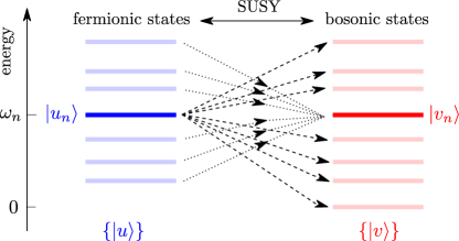
Figure 27: SUSY contribution to the bosonic Berry curvature. The SUSY contribution to the bosonic Berry curvature consists of two distinct transitions between the fermionic vector space $\{|u\rangle\}$ (blue) and the bosonic vector space $\{|v\rangle\}$ (red): (i) $|u_{n}\rangle\rightarrow|v_{m\neq n}\rangle$ shown in dashed arrows and (ii) $|u_{m\neq n}\rangle\rightarrow|v_{n}\rangle$ shown in dotted arrows (detailed in the text).

Berry Curvature. Similarly, one can study how the Berry curvature is related for bosonic and fermionic tight-binding models that are connected by such a supersymmetric identification. For a given (isolated) fermionic band $|u_{n}\rangle$ in the spectrum of ${\cal H}_{F}\equiv{\bf RR^{\dagger}}$ the Berry curvature can be cast as

$${\cal F}_{n}^{(u)}({\bf k})=-2\leavevmode\nobreak\ {\rm Im}\Bigg{[}\sum_{m\neq n}\frac{\langle u_{n}|\partial_{x}{\cal H}_{F}|u_{m}\rangle\langle u_{m}|\partial_{y}{\cal H}_{F}|u_{n}\rangle}{(\omega_{n}-\omega_{m})^{2}}\Bigg{]},$$ (73)

where $\partial_{i}\equiv\partial/\partial k_{i}$. Then the corresponding supersymmetric bosonic partner state in the spectrum of ${\cal H}_{B}\equiv{\bf R^{\dagger}R}$ given by $|v_{n}\rangle$ will have a Berry curvature of

$${\cal F}_{n}^{(v)}({\bf k}) ={\cal F}_{n}^{(u)}({\bf k})$$

$$+2\leavevmode\nobreak\ {\rm Im}\Bigg{[}\sum_{m\neq n}\frac{\langle v_{n}|\partial_{x}{\bf R}^{\dagger}|u_{m}\rangle\langle u_{m}|\partial_{y}{\bf R}|v_{n}\rangle}{(\omega_{n}-\omega_{m})}$$

$$\leavevmode\nobreak\ \leavevmode\nobreak\ \leavevmode\nobreak\ -\sum_{m\neq n}\frac{\langle u_{n}|\partial_{x}{\bf R}|v_{m}\rangle\langle v_{m}|\partial_{y}{\bf R}^{\dagger}|u_{n}\rangle}{(\omega_{n}-\omega_{m})}\Bigg{]}\,,$$ (74)

which like the Berry phase above is found to be augmented by an additional term.

The expression in (73) formally resembles the result of a second-order perturbation theory calculation. It is a gauge-invariant form of the Berry curvature that admits contributions owing to the transitions from all other bands to the given $n$-th band considering $\partial_{i}{\cal H}$ as a perturbation. In a similar spirit, one can inspect the supersymmetric contribution in (E) which reveals two noteworthy features. Firstly, the supersymmetric contribution recognizes $\partial_{i}{\bf R}$ and $\partial_{i}{\bf R}^{\dagger}$, i.e., derivatives of the supercharges, as first-order perturbations. The conventional term instead concerns the derivative of the fermionic Hamiltonian $\partial_{i}{\cal H}_{F}$ as second-order perturbations instead. Secondly, the supersymmetric contribution comprises two complementary components signifying two distinct types of transitions (admixing the bosonic and fermionic Hilbert spaces) – the first term in the square bracket in (E) is due to the transitions from the bosonic Bloch state $|v_{n}\rangle$ to all eigenvectors in the vector space of its fermionic superpartner indexed with $m\neq n$, as schematically illustrated in Fig. 27. In contrast, the second term is due to the transitions from the fermionic eigenvector $|u_{n}\rangle$ (the superpartner of $|v_{n}\rangle$) at the same energy $\omega_{n}$, to all the eigenvectors in the bosonic vector space $\{|v\rangle\}$ indexed with $m\neq n$. Similar to what we have seen for the Berry phase above, it turns out that in the honeycomb-kagome correspondence, when we gap out the Dirac cones with a small inversion symmetry breaking parameter to isolate the uppermost band in both cases, these two terms nullify each other rendering the fermionic and bosonic Berry curvatures identical ${\cal F}^{(v)}({\bf k})={\cal F}^{(u)}({\bf k})$.

De facto, it seems that for the SUSY connection of complex fermions and bosons discussed here, there is no distinction of the SUSY version of the Berry phase and its original variant and similarly for the Berry curvature. At least this is what we find for a number of examples discussed in Section III. A completely different picture awaits us when we turn to the case of real fermions and bosons, which we discussed in Section IV, in the context of topological mechanics.

Appendix F Kane-Lubensky chain to Kitaev chain

Let us complement the discussion of the SUSY correspondence of one of our principal examples in topological mechanics, between the (bosonic) Kane-Lubensky chain and the (fermionic) Kitaev chain, in the main text by a more detailed derivation here. In particular, let us demonstrate how to derive a local compatibility matrix $\tilde{\bf A}$ of the form given in (57) (of the main text) from the Kane-Lubensky dynamical matrix

$$\tilde{\bf D}=\begin{pmatrix}a&b&0&0&\dots&b\\ b&a&b&0&\dots&0\\ 0&b&a&b&\dots&0\\ \vdots&\vdots&\vdots&\vdots&\vdots&\vdots\\ 0&0&\dots&b&a&b\\ b&0&0&\dots&b&a\end{pmatrix}\equiv\tilde{\bf A}^{T}\tilde{\bf A}\,,$$ (75)

that enables constructing a Kitaev chain as a superpartner of the phonon problem. The strategy is to first construct an incidence matrix of the graph represented by the phonon chain which entails interactions up to the next nearest neighbors as reflected in $\tilde{\bf D}$, thereby retaining the features of locality same as $\tilde{\bf D}$. This is important to construct a local fermionic Hamiltonian via our SUSY approach. It provides a simple mathematical demonstration of the graph square-rooting algorithm presented earlier applied to formulate supersymmetric partners of random nearest-neighbor one-dimensional bosonic models.

To proceed, the first step is to project out the diagonal terms of $\tilde{\bf D}$ to construct a weighted adjacency matrix that contains the connectivities (including the bond strengths) between distinct sites of the phonon chain. Note the parameters $a,b$ in (75) are arbitrary positive numbers representing a generic one-dimensional phonon model with an adjacency matrix

$$\tilde{\cal A}=\begin{pmatrix}0&b&0&0&\dots&b\\ b&0&b&0&\dots&0\\ 0&b&0&b&\dots&0\\ \vdots&\vdots&\vdots&\vdots&\vdots&\vdots\\ 0&0&\dots&b&0&b\\ b&0&0&\dots&b&0\end{pmatrix}.$$ (76)

Regarding the underlying phonon lattice as a one-dimensional graph with connectivities between next nearest neighboring sites only, the incidence matrix induces a map from the sites, denoted by $\{i\}$, to the bonds of this graph, denoted by $\{\alpha\}$, which we can write as

$$\tilde{\cal I}=\begin{pmatrix}x_{1}\sqrt{b}&\sqrt{b}/x_{1}&0&0&\dots&0\\ 0&x_{2}\sqrt{b}&\sqrt{b}/x_{2}&0&\dots&0\\ 0&0&x_{3}\sqrt{b}&\sqrt{b}/x_{3})&\dots&0\\ \vdots&\vdots&\vdots&\vdots&\vdots&\vdots\\ \sqrt{b}/x_{N}&0&0&\dots&0&x_{N}\sqrt{b}\end{pmatrix}$$ (77)

for a periodic $N$-site (and $N$-bond) isostatic chain. We then determine the parameters $\{x_{\alpha}\}$, which is a set of $N$ real-valued numbers on the bonds, by imposing the condition

$$\tilde{\cal I}^{T}\tilde{\cal I}=b\begin{pmatrix}f_{1}&1&0&0&\dots&1\\ 1&f_{2}&1&0&\dots&0\\ 0&1&f_{3}&1&\dots&0\\ \vdots&\vdots&\vdots&\vdots&\vdots&\vdots\\ 0&0&\dots&1&f_{N-1}&1\\ 1&0&0&\dots&1&f_{N}\end{pmatrix}=\tilde{\bf D}$$ (78)

with $f_{\alpha}=x_{\alpha}^{2}+1/x_{\alpha}^{2}$ or, equivalently,

$$x_{\alpha}^{2}+1/x_{\alpha}^{2}=a/b,$$ (79)

that has four solutions

$$x_{i}=\pm\sqrt{\frac{a}{2b}\pm\sqrt{\frac{a}{2b}-1}},$$ (80)

independent of $\alpha$, leading to the $N\times N$ compatibility matrix $\tilde{\bf A}$ noted in (57) of the main text.