LOTUS: A (non-)LTE Optimization Tool for Uniform derivation of
Stellar atmospheric parameters

Abstract

Precise fundamental atmospheric stellar parameters and abundance determination of individual elements in stars are important for all stellar population studies. Non-Local Thermodynamic Equilibrium (Non-LTE; hereafter NLTE) models are often important for such high precision, however, can be computationally complex and expensive, which renders the models less utilized in spectroscopic analyses. To alleviate the computational burden of such models, we developed a robust 1D, NLTE fundamental atmospheric stellar parameter derivation tool, LOTUS, to determine the effective temperature $T_{\rm eff}$, surface gravity $\log g$, metallicity [Fe/H] and microturbulent velocity $v_{\mathrm{mic}}$ for FGK type stars, from equivalent width (EW) measurements of Fe i and Fe ii lines. We utilize a generalized curve of growth method to take into account the EW dependencies of each Fe i and Fe ii line on the corresponding atmospheric stellar parameters. A global differential evolution optimization algorithm is then used to derive the fundamental parameters. Additionally, LOTUS can determine precise uncertainties for each stellar parameter using a Markov Chain Monte Carlo (MCMC) algorithm. We test and apply LOTUS on a sample of benchmark stars, as well as stars with available asteroseismic surface gravities from the K2 survey, and metal-poor stars from the $Gaia$-ESO and $R$-process Alliance (RPA) surveys. We find very good agreement between our NLTE-derived parameters in LOTUS to non-spectroscopic values on average within $T_{\rm eff}$ $=\pm 30$ K and $\log g$ $=\pm 0.10$ dex for benchmark stars. We provide open access of our code, as well as of the interpolated pre-computed NLTE EW grids available on Github github, and documentation with working examples on Readthedocs book.

1 Introduction

Precise characterization of stellar spectra is a key ingredient for understanding several fields of modern astrophysics, including the physical and chemical properties and abundances of stars (Asplund et al., 2009; Jofré et al., 2019), galactic formation and evolution (Audouze & Tinsley, 1976; McWilliam, 1997; Kobayashi et al., 2006), as well as macro and micro physical phenomena near the surface of stars (Miesch & Toomre, 2009; Linsky, 2017). This accurate level of characterization is also needed for the detection of extra-solar planets when using radial velocity methods (Vanderburg et al., 2016).

With the current inflow of stellar spectra from ongoing and future large observational spectroscopic surveys including, SDSS-V (Kollmeier et al. 2017, R$\sim$2000 and $\sim$22500), LAMOST (Liu et al. 2020, R$\sim$7500; Cui et al. 2012; Zhao et al. 2012; Deng et al. 2012, R$\sim$1800), APOGEE (Ahumada et al. 2020, R$\sim$22500), RAVE (Steinmetz et al. 2020, R$\sim$7500), GALAH (De Silva et al. 2015, R$\sim$28000), as well as the upcoming WEAVE (Dalton et al. 2016, R$\sim$5000 and R$\sim$20000), 4MOST (de Jong et al. 2019, R$\sim$20000) and PLATO (Miglio et al. 2017), stellar spectroscopy will be providing $\sim 10^{5}$ of golden opportunities to study the chemical and dynamical properties of stars in the Galaxy to help understand its build-up history and evolution.

Atmospheric fundamental stellar parameters, including the effective temperatyre $T_{\rm eff}$, surface gravity $\log g$, metallicity [Fe/H] and microturbulent velocity $v_{\mathrm{mic}}$, as well as chemical abundances of stars, are determined from the observed spectra of a given star by fitting theoretical synthetic spectra based on assumptions of geometric structures (1D versus 3D), radiative transfer assumptions (Local Thermodynamic Equilibrium; hereafter LTE, versus Non-Local Thermodynamic Equilibrium; hereafter NLTE). Two classical methods are commonly used to derive stellar atmospheric parameters from stellar spectra: either 1) by iteratively fitting the observed spectra to synthetic spectral models until a best-fit match is met at the corresponding stellar parameters, or 2) by measuring chemical abundances determined from Fe i and Fe ii lines from equivalent widths (EW) measurements, and employing optimization of excitation and ionization equilibrium by changing the stellar parameters iteratively until trends with excitation potential energies ($\chi$) and reduced equivalent widths ($\log(EW/\lambda)$) of the lines are minimized. While the former method of spectral synthesis might outperform the latter in crowded spectral regions or spectra dominated by strong lines ($\log(EW/\lambda)>-4.5$), the EW method generally requires less calculation time and resources than synthetic spectra, making it a simpler and more widely applied tool to measure atmospheric stellar parameters and chemical abundances.

Classical radiative transfer models for deriving stellar parameters and chemical abundances from observed spectra most often LTE. Under LTE, the gas and chemical particles throughout the stellar atmosphere satisfy the Saha-Boltzmann excitation and ionization balance equations. Several stellar atmospheric parameter tools implementing classical 1D and LTE approximations for spectroscopic analyses already exist and are widely used (e.g., MATISSE (Recio-Blanco et al., 2006), MyGIsFOS (Sbordone et al., 2014), the APOGEE pipeline ASCAP (García Pérez et al., 2016), GALA (Mucciarelli et al., 2013), DOOp (Cantat-Gaudin et al., 2014), ARES (Sousa et al., 2015), StePar (Tabernero et al., 2019), FASMA (Tsantaki & Andreasen, 2021) and iSpec (Blanco-Cuaresma et al., 2014; Blanco-Cuaresma, 2019).

The LTE assumption utilized by all of these tools is, however, not physically motivated when applied to evolved giants and/or metal-poor stars (Lind et al., 2012; Ezzeddine et al., 2017; Mashonkina et al., 2017; Amarsi et al., 2020). Inelastic collisional interactions between atoms and electrons or neutral hydrogen in the atmospheres of cool stars usually drive the local conditions in these atmospheres towards LTE. In metal-poor and giant stars, limited electron donors from metals are not able to induce enough collisions to maintain collisional equilibrium in the line-forming regions (Hubeny & Mihalas, 2014), which drive line formation away from LTE (Mihalas & Athay, 1973; Bergemann et al., 2012). Quantified deviations in abundances and stellar atmospheric parameters from LTE are commonly known as NLTE effects (Asplund, 2005), which are mainly driven by deviations from statistical equilibrium or kinematic equilibrium.

A small number of radiative transfer codes have started taking NLTE effects into account for the determination of chemical abundances, including PySME (Wehrhahn, 2021), which is based on the spectroscopic analysis code Spectroscopy Made Easy (SME; Piskunov & Valenti 2017). Kovalev et al. (2019) has implemented NLTE departure coefficients in the synthesis tools, allowing NLTE spectral synthesis for certain corresponding absorption lines. More recently, a NLTE version of Turbospectrum (Plez, 2012) has been released (Gerber et al., 2022), which also has NLTE departure coefficients incorporated in their 1D, LTE spectral synthesis models. However, both codes allow NLTE corrections for only some elements via spectral synthesis, and stellar parameters still need to be derived independently or iteratively via full spectral fitting, which can be prone to degeneracies. Therefore, a tool that can automatically derive stellar parameters incorporating NLTE models, taking into account stellar parameter dependencies, is highly needed which is the main motivation of this work and paper.

In this work, we present a fast, automatic and robust spectroscopic analysis tool, LOTUS, which stands for a “(non-)LTE Optimization Tool for Uniform derivation of Stellar atmospheric parameters”. LOTUS allows the derivation of $T_{\rm eff}$, $\log g$, [Fe/H] and $v_{\mathrm{mic}}$ based on EW measurements input of Fe i and Fe ii lines from stellar spectra. Either or both LTE and NLTE modes can be chosen for the benefit of comparisons. As compared to traditional full NLTE calculations for each model, LOTUS can significantly shorten the time of the determination of stellar parameters using the NLTE assumption from several hours or even days (Hauschildt et al., 1997) to $\sim 15-30$ mins for each star. A Monte-Carlo Markov Chain (MCMC) analysis is also implemented to precisely estimate the uncertainties of the derived parameters. We test and apply LOTUS on several benchmark stars, and stellar surveys with available non-spectroscopic atmospheric parameters (from asteroseismology or interferometry)for comparison and validation of our results.

The rest of the paper is organized as follows: In Section 2, we present a detailed description of LOTUS, and describe the input models for our NLTE calculations, as well as a description of the different modules of the code. In Section 3, we test our code and apply it to derive and compare the derived parameters of benchmark stars, and stars with non-spectroscopic derived parameters. In Section 4, we apply the code to a large sample of metal-poor stars and discuss the NLTE effects obtained via LOTUS. In Section 5, we present a discussion on the caveats and limitations of the code, and finally, in Section 6 we present a summary of our results and conclude.

2 General description

LOTUS is designed to derive the fundamental atmospheric stellar parameters $T_{\rm eff}$, $\log g$, [Fe/H] and $v_{\mathrm{mic}}$of FGK type stars, by implementing observed measurements of EW for Fe i and Fe ii lines as input. An example of a user input EW linelist is shown in Listing 1 below. The transition wavelength (obs_wavelength in Å), element and ionization stage (Fe i or Fe ii), measured EW (obs_ew in mÅ) and excitation potential energy EP (obs_ep in eV) are required.

⬇

1obs_wavelength,element,obs_ew,obs_ep

24787.8266,FeI,44.2,3.00

34788.7566,FeI,65.5,3.24

44789.6508,FeI,83.3,3.55

56456.3796,FeII,59.2,3.9

6...

Listing 1: Example of an input file format of observed EW measurements for Fe i and Fe ii lines provided by users for LOTUS. obs_wavelength are in Å, obs_ew in mÅ, and obs_ep in eV.

LOTUS has three general modules of functionality. In a general overview, (i) Fe i and Fe ii abundances are derived by interpolating a generalized curve of growth (GCOG) for each line in a pre-computed grid of theoretical EW in both LTE and NLTE, following Boeche & Grebel (2016). (ii) the stellar parameters are then derived by minimizing the slopes for excitation and ionization equilibrium, iteratively using a global minimization module, and finally, (iii) uncertainties of the derived atmospheric parameters are estimated utilizing a Markov Chain Monte Carlo (MCMC) algorithm. We describe each of these modules in detail in sub-section 2.2 below, after listing the input and radiative transfer models used in Section 2.1.

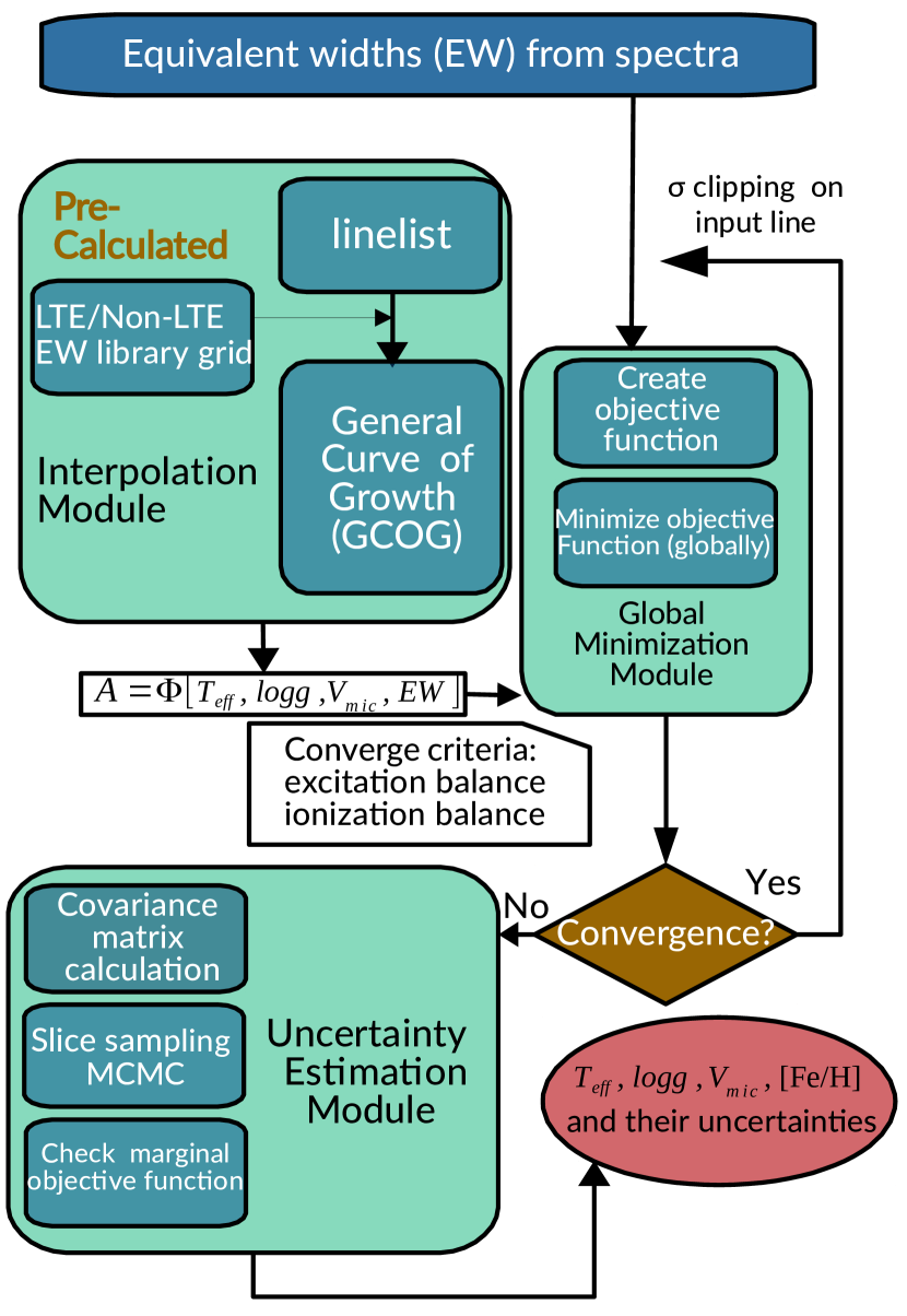
Figure 1: A flow diagram describing the working modules of LOTUS. Three main modules are used to derive the stellar parameters and their uncertainties: (i) an interpolation Module, (ii) a Global Minimization Module, and (iii) an Uncertainty Estimation Module. Input includes EW measurements of Fe i and Fe ii of the absorption lines measured in the spectra. Users can define the number of $\sigma$ clipping required to remove outliers (see Section 2.4.3 for details). Additionally, a halt condition for the value of the smallest allowable minimization function threshold can also be defined by users (see Section 2.4.3 for details).

2.1 Input Models

2.1.1 Stellar Atmosphere Models

LOTUS incorporates 1D, LTE MARCS stellar atmospheric models (Gustafsson et al., 1975, 2008), covering a wide range of stellar parameters typical for FGK stars.

Spherical atmospheric models were used for $\log g$$\,<3.5$, otherwise, plane-parallel models were adopted. The grid of MARCS model atmosphere available online offers reasonable coverage for the stellar parameters, however they exhibit wide gaps in effective temperature (steps of $\sim 250$ K), surface gravity (steps of $\sim 0.5$ cgs), and metallicity (steps of $\sim 0.25-0.50$ dex) to optimally explore the parameter space. We utilize the MARCS interpolation subroutine iterpol_marcs.f written by Thomas Masseron, to produce a higher resolution grid, with our final parameter grid ranging from 4000 K to 6850 K for $T_{\rm eff}$ (steps of 50 K), $\log g$ from 0.0 to 5.0 (steps of 0.1), [Fe/H] from $-3.5$ to $+0.5$ (steps of 0.5) and $v_{\mathrm{mic}}$ from 0.5 to 3.0 km s^-1 (steps of 0.5 km s^-1).

2.1.2 Iron Model Atom

Computing theoretical NLTE Fe i and Fe ii EWs requires the input of a comprehensive iron model with up-to-date radiative and collisional atomic data. For our EW grid calculations, we adopt a well-tested Fe i/Fe ii model atom containing 846 Fe i and 1027 Fe ii lines Ezzeddine et al. (2016, 2017, 2020). The atom includes absorption line transitions spanning the near-UV to the near-IR, extending the range of wavelength from $\sim 1000$ to $10^{5}$ Å. The model also carefully considers hydrogen collision and electron collision processes from quantum atomic data, particularly implementing ion-pair production and mutual-neutralization processes from Barklem (2018). Extensive details on the build-up of the atom and the corresponding atomic data are presented in Ezzeddine et al. (2016) and Ezzeddine et al. (2020).

2.1.3 NLTE Radiative Transfer computations

We utilized the NLTE radiative transfer code MULTI2.3 to solve for statistical equilibrium populations and derive the theoretical NLTE EW for the Fe i and Fe ii lines in our atom. The code utilizes the Approximate Lambda Iteration (ALI) (Rybicki & Hummer, 1991) to iteratively determine the populations using the comprehensive Fe i/Fe ii model atom described in Section 2.1.2. MULTI2.3 also solves for LTE populations using the classical Saha and Boltzmann equations, which is output as a departure coefficient, $b_{i}$, where $b_{i}=n_{i}(\mathrm{NLTE})/n_{i}(\mathrm{LTE})$ (Wijbenga & Zwaan, 1972), where $n$ is the level population for the corresponding line transition $i$.

2.1.4 Linelist Selection

The linelist selection is crucial for the accurate derivation of Fe i and Fe ii chemical abundances and stellar parameters using the EW method, especially for cooler stars (e.g. FGK stars) since they have much denser spectral line regions containing blended lines. Therefore, we choose a comprehensive list of Fe i and Fe ii from the $Gaia$-ESO line list (Jofré et al., 2014; Heiter et al., 2015, 2021), covering the wavelength ranges from 4750 to 6850 Å and from 8500 to 8950 Å. Additional lines from the R-Process Alliance (RPA) survey (e.g., Hansen et al., 2018; Sakari et al., 2018; Ezzeddine et al., 2020; Holmbeck et al., 2020) have also been added to account for lines common in metal-poor stars, with corresponding atomic data and references in (Roederer et al., 2018). We combine iron lines from both linelists, removing any duplicates in the process. Our final linelist is presented in Table 2. Future LOTUS releases should be easily able to extend the linelists to bluer and redder lines in the UV and IR, respectively.

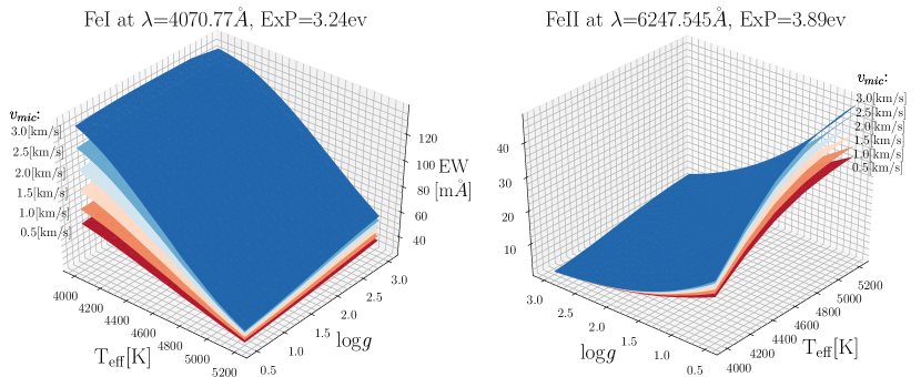
Figure 2: Computed NLTE EW dependence as a function of $T_{\rm eff}$, $\log g$, $v_{\mathrm{mic}}$ for the Fe I line at 4070.77Å and EP=3.24 eV (left) and the Fe II line at 6247.55$\AA$ with EP=3.89 eV (right). Both lines have been computed at a fixed [Fe/H]$=-2.0$.

2.2 Key Modules

Below we describe in detail the key components and modules of the LOTUS functionalities. An illustrated flow diagram of the workings of the code is also shown in Figure 1, demonstrating the connection between the different modules.

2.2.1 EW Interpolation Module

Traditional curve of growth (COG) methods to derive chemical abundances usually employ simplistic models, typically computed at fixed $T_{\rm eff}$, $\log g$, [Fe/H] and $v_{\mathrm{mic}}$ for each line. For some lines, however, EW can have strong dependencies on multiple atmospheric stellar parameters in a given parameter space. Figure 2 demonstrate these dependencies, where EW variation from our computed NLTE grid are shown as a function of $T_{\rm eff}$ $\log g$ and $v_{\mathrm{mic}}$ for the Fe I line at 4070.768 Å (left panel), and the Fe II lines at 6247.545 Å (right panel), respectively. The metallicity for both plots has been fixed at [Fe/H] $=-2.00$ for demonstration purposes. We observe that at a fixed [Fe/H], increasing $T_{\rm eff}$ will decrease EW of the Fe i line, while EW being mostly insensitive to $\log g$ variation; For Fe ii lines, however, increasing $T_{\rm eff}$ will increase EW while increasing $\log g$ will decrease EW. For both lines, EW will increase as $v_{\mathrm{mic}}$ increases, as $v_{\mathrm{mic}}$ delays the saturation by spreading absorption into a wider wavelength band. These EW-stellar parameter dependencies have been qualitatively proven in Chapter 17.5 of Hubeny & Mihalas (2014). Thus, to take into account such important dependencies in our codes, which can affect our derived abundances and thus our stellar parameter derivation, we compute a Generalized Curve of Growth (GCOG) for each Fe i and Fe ii line in our linelist. We define the GCOG for any given line $i$ as:

$$GCOG_{i}\mathpunct{:}\left(T_{\mathrm{eff}},\mathrm{log}\textit{g},\nu_{mic},\mathrm{EW}\right)\mapsto A(\mathrm{Fe})_{i}$$

A GCOG is thus a generalization of the well-known COG onto a higher dimensional mapping of EW $\mapsto$ A(Fe) Alternatively, COG_i can be obtained by fixing $T_{\rm eff}$  $\log g$  and $v_{\mathrm{mic}}$ for a given GCOG. GCOGs have been implemented in previous studies such as Osorio et al. (2015) and Boeche & Grebel (2016). We thus provide interpolated GCOGs which are stored as libraries in our code for every line in our linelist (see Section 2.1.4).The GCOGs are then utilize in the optimization module afterward to derive the Fe i and Fe ii abundances.

2.3 Abundance Determination module

To derive the Fe i and Fe ii abundances, we fit multivariate polynomials to the GCOG of each line, by deriving the relationship between the iron abundance of the line with $T_{\rm eff}$, $\log g$, $v_{\mathrm{mic}}$ and EW, denoted as $A\left(\mathrm{Fe}\right)=P\left(T_{\mathrm{eff}},\mathrm{log}\textit{g},\nu_{mic},\mathrm{EW}\right)$. The detailed form of $P$ can be written as:

$$\sum_{i_{1}+i_{2}+i_{3}+i_{4}\leq n}a_{i_{1}i_{2}i_{3}i_{4}}\left(T_{\mathrm{eff}}\right)^{i_{1}}\left(\mathrm{log}\textit{g}\right)^{i_{2}}\left(v_{mic}\right)^{i_{3}}\left(\mathrm{EW}\right)^{i_{4}}$$ (1)

where $i_{m}$ ($m=1,2,3,4$) is the polynomial power of each of the 3 stellar parameters ($T_{\rm eff}$, $\log g$ and $v_{\mathrm{mic}}$) as well as EW. Possible values for $i_{m}$ are positive integers, where the sum of all the powers should less than or equal to the power degree of the polynomial $n$. $a_{i_{1}i_{2}i_{3}i_{4}}$ is the product of the polynomial coefficients of all the variables. The criteria for choosing $n$ depends on the behavior of theoretical GCOG models within a range of stellar parameters and is described in more details in Section 2.3.1 below.

Table 1: Interpolation intervals chosen for different stellar types considered in LOTUS.

stellar parameter	types	intervals
T${}_{\textrm{eff}}$ (K)	K	[4000, 5200]
	G	[5200, 6000]
	F	[6000, 6850]
logg	supergiant	[0.0, 0.5]
	giant	[0.5, 3.0]
	subgiant	[3.0, 4.0]
	dwarf	[4.0, 5.0]
[Fe/H]	very metal poor	[$-3.5$, $-2.0$]
	metal poor	[$-2.0$, $-0.5$]
	metal rich	[$-0.5$, 0.5]

2.3.1 Selection of Interpolator

We choose the linelist utilized to derive stellar parameters to be dependent on the spectral type of the star, as some lines can be blended or strong in cool high metallicity stars, whereas these same lines could also be blend-free and weaker for hotter, metal-poor stars. Therefore, the multivariate polynomial functions defined in Section 2.3 used to derive the abundances determined from Fe i and Fe ii lines depend on the choice of linelist for each spectral type. We thus pay special attention to the choice of interpolator by identifying the best selection of linelist per spectral type (or stellar parameters). Therefore, instead of interpolating in the whole parameter space for all the lines, we pre-define that the GCOGs fit only the abundances determined from the lines we pre-selected and chose to use within tested intervals of stellar parameters, according to an initial guess of spectral types that the users can insert as an input in the code. Our choice of the intervals of different stellar parameters for each spectral types are listed in Table 1. For example, if an initial guess is chosen such that the target star is a metal-poor G giant, the multivariate polynomial will fit the abundance of each line versus other atmospheric parameters using the grid points falling into the range of $T_{\rm eff}$ from 5200 K to 6000 K, $\log g$ from 0.0 to 3.0 and [Fe/H] from $-2.0$ to $-0.5$.

In order to choose the best interpolator per spectral type (i.e., the optimal $n$) among several multivariate polynomials as defined in Equation 1, we use a Bayesian Information Criteria (BIC) to select the best polynomial function for each line based on the mean residual differences between the theoretical EWs at the nodes of our pre-computed NLTE grid (computed at a combination of $T_{\rm eff}$, $\log g$, [Fe/H], and $v_{\mathrm{mic}}$), to the EWs interpolated at these parameters. We assume that the optimal model is among the polynomials with degree=2,3,4,5. The BIC was calculated such as:

$$\mathrm{BIC}=n\,\mathrm{ln}\left(\frac{\mathrm{SSR}}{n}\right)+k\,\mathrm{ln}(n)$$ (2)

where SSR is the sum of the squared residuals between the theoretical EWs and the interpolated EWs from models at specific nodes of the grid, and $n$ is sample size (here we choose $n=4000$ nodes in each spectral type interval). $k$ is a free parameter (including coefficients and slope intercept), which can be calculated as k=$C_{d+4}^{d}$, where $d$ is the degree of the polynomial, and 4 is chosen as the number of dependent variables for each interpolated EW (namely, $T_{\rm eff}$, $\log g$, [Fe/H] and $v_{\mathrm{mic}}$).

We thus chose the best interpolator for each spectral type interval as that with the lowest BIC value. In Fig. 3, we show the differences between the interpolated EW using the lowest BIC interpolator as compared to the (non-interpolated) EW directly from MULTI2.3, categorized as a function of stellar spectral types (x-axis) and metalicities (different panels). We observe that there exist no clear dependencies between differences and spectral types and metalicities. The average of differences is within 0.01 for all stellar spectral types and metalicities. We pre-define the default interpolated EW uncertainty (also a threshold for the lowest acceptable BIC) in LOTUS as 6 m$\AA$ for each line. However, we also design the code to allow users to input their acceptable uncertainty limits, in which case LOTUS will drop a given Fe i or Fe ii from the linelist if the computed BIC is larger than this uncertainty, and will subsequently be excluded from the lines used to derive the stellar parameters in the optimization module.

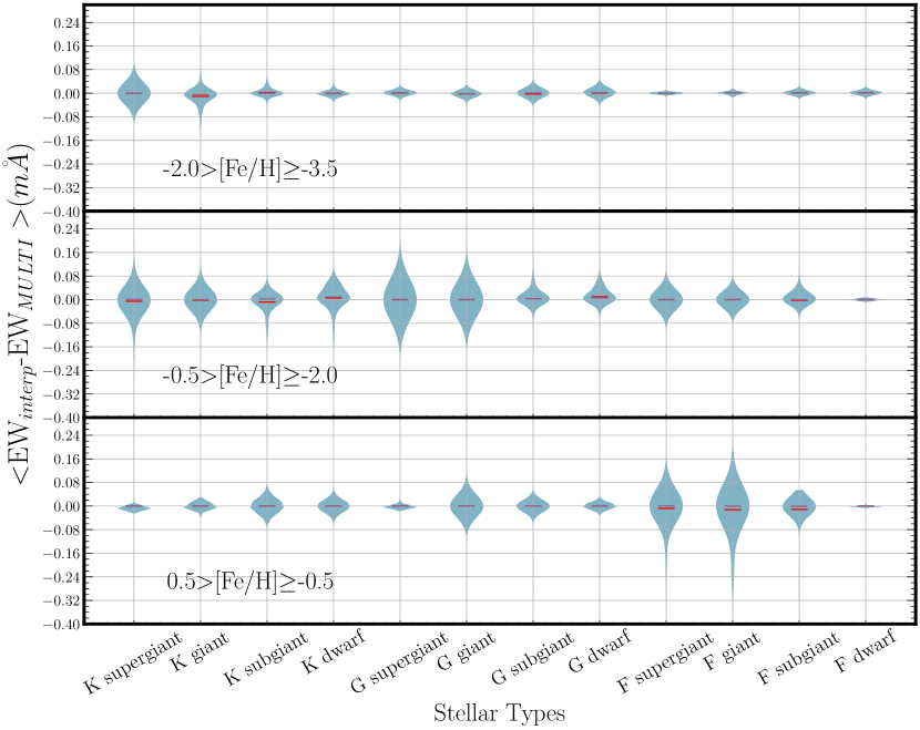
Figure 3: Differences (in mÅ) between the interpolated EWs (using interpolators chosen at the lowest BIC values) and the EWs from NLTE theoretical calculations computed directly using MULTI2.3. Each violin plot shows the distribution of the means of such differences for a random 4000 nodes within the spectral type interval of the pre-computed EW library. Red lines are marked as the means of the distributions while purple lines are for the medians. The differences are shown for different metallicity ranges as indicated in each panel.

2.3.2 EP Cut-off

The NLTE abundances derived from low excitation potential Fe i can yield larger abundances as compared with those derived from high-excitation Fe i and Fe ii lines, especially using 1D atmospheric models (Amarsi et al., 2016). Such differences can reach up to 0.45 dex for some Fe i lines, and can affect our derived stellar parameters as documented in several studies including Bergemann et al. (2012); Lind et al. (2012) as well as others. We thus follow previous literature studies by introducing low-excitation potential cut-offs for Fe i lines with EP(Fe i) $<$ 2.7ev/2.5ev/2.0 eV for stars with [Fe/H]$<-0.5$, depending on the number of Fe i and Fe ii lines measured in the stars and the optimization convergence criteria (see Section 2.4); We conduct no cut-offs for stars with [Fe/H]$>-0.5$.

2.4 Optimization Module

Once reliable linelist and interpolators per spectral types of input target stars have been chosen, as explained in Section 2.3 above, the derived iron abundances from Fe i and Fe ii lines are fed into the optimization module with an initial guess of the general type of the target star. We note that users don’t need to specify an initial guess of each stellar parameter, as it suffices to only chose an initial guess of the spectral type as an input to LOTUS, which is then assigned the corresponding interpolation parameters interval as indicated in Table 1.

2.4.1 Optimization Conditions

The general principle of optimization is to adjust stellar parameters iteratively to derive optimal combinations of stellar parameters that can satisfy the following three conditions: (i) excitation equilibrium, or minimizing the trend (i.e., slope) of the Fe i abundances as a function of excitation potential EP, (ii) ensuring ionization equilibrium or minimizing the differences between the abundances derived from the Fe i and Fe ii lines, and (iii) minimizing the trend (i.e., slope) between the abundances derived from the Fe i lines versus the reduced equivalent widths, REW = $\log(\mathrm{EW}/\lambda)$.

Therefore, we derive $T_{\rm eff}$ by ensuring excitation equilibrium, $\log g$ by ensuring ionization equilibrium, and $v_{\mathrm{mic}}$ by minimizing the trend between Fe i abundances versus line strength (REW). [Fe/H] was then determined by averaging the abundances derived from the Fe i and Fe ii abundances.

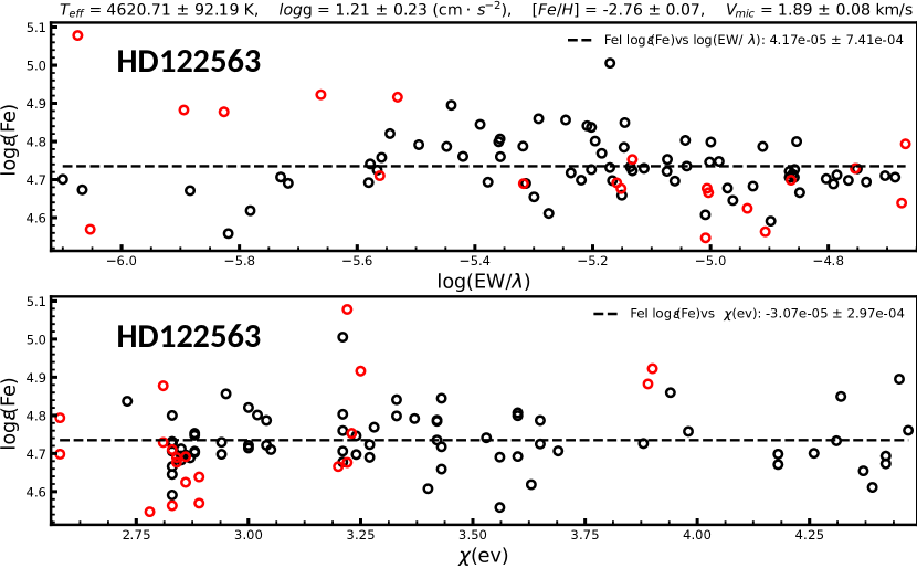
Figure 4: Iron abundances determined from Fe i (black circles) and Fe ii (red circles) line versus reduced equivalent widths (upper panel) and excitation potential energies $\chi$ (lower panel) for selected lines in the metal-poor benchmark star HD122563. The parameters indicated on the top are the optimal values derived using the global minimization (differential evolution) algorithm in LOTUS. Dotted lines are the best linear fits to the Fe i lines in each panel. The labels at the upper left corner of each panel are the slopes of the fits and their corresponding standard deviations.

2.4.2 Targeted Optimized Object Function

In order to find the best combination of stellar parameters that satisfy the optimization conditions defined in Section 2.4.1 within our parameter grid, we first combine these conditions into an object function $\mathcal{F}$, such as:

$$\mathcal{F}=\left(\frac{s_{\chi,1}}{\sigma_{\chi,1}}\right)^{2}+\left(\frac{s_{REW,1}}{\sigma_{REW,1}}\right)^{2}+\left(\frac{\bar{A_{1}}-\bar{A_{2}}}{\sigma_{1-2}}\right)^{2}$$ (3)

where the subscripts ”1” and ”2” correspond to Fe i and Fe ii, respectively. $s_{\chi,1}$ is the slope between Fe i abundances and EP, and $\sigma_{\chi,1}$ is its uncertainty, $s_{REW,1}$ is the slope between the Fe i abundances and REW, and $\sigma_{REW,1}$ is its uncertainty. $\bar{A_{1}}$ and $\bar{A_{2}}$ are the mean abundances for Fe i and Fe ii, respectively, while $\sigma_{1-2}$ is the standard deviation of the differences between $\bar{A_{1}}$ and $\bar{A_{2}}$. A converged solution is obtained at the combination of $T_{\rm eff}$, $\log g$, [Fe/H] and $v_{\mathrm{mic}}$, which minimizes $\mathcal{F}$ globally.

2.4.3 Global minimization

To find the global minimization fit parameters within our grid, we adopt a differential evolution algorithm implementing a global minimization search. The goal is to minimize $\mathcal{F}$ by starting with an initial population of candidate solutions, which are iteratively improved by retaining the fittest solutions that yield a lower $\mathcal{F}$ values, until convergence for the best-fit parameters is met (Storn & Price, 1996). The advantage of a differential evolution algorithm is that it has the benefit of handling nonlinear and non-differentiable multi-dimensional objective functions while requiring few control parameters to steer the minimization. For our code, we select 100 initial populations (sets of solutions) with a combined rate of 0.3, which is a crossover probability that depends on how fast the algorithm moves to the next generation of populations. We try different weights between 0.8 and 1.2, to maintain a proper searching radius, at the same time making sure it does not slow down the convergence speed. We adopt $\mathcal{F}\sim 10^{-5}$ as the absolute tolerance for each iteration. After each iteration, we perform a 3$\sigma$-clipping on the abundances determined from the Fe i and Fe ii lines to remove outliers. We adopt 3 iterations of outlier removing in total as a default, however, this number can be defined by the users depending on the quality of their EW measurements. An example of HD122563 with derived abundances of Fe i and Fe ii versus REW and EP at optimal atmospheric parameters is shown in Figure 4.

2.5 Uncertainty Estimation Module

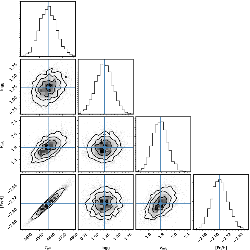
Figure 5: Marginalized posterior distributions of the stellar parameters of HD122563 based on the log-likelihood function in Equation 6. 1$\sigma$, 2$\sigma$ and 3$\sigma$ uncertainty region are denoted as solid contours in the two dimensional plot. The histograms show the marginalized posterior distributions for each parameter, respectively. Blue intersecting lines show the values obtained from our global optimization module.

Since $\mathcal{F}$ is a function of the stellar parameters, it can be described as $\mathcal{F}(\theta)=\mathcal{F}(T_{\mathrm{eff}},log\mathrm{g},$$v_{\mathrm{mic}}$$)$. We can keep track of how $\mathcal{F}$ changes along the perturbations around the optimal solution $\theta^{*}$=($T_{\mathrm{eff}}^{*}$, log$\textit{g}^{*}$, $v_{\mathrm{mic}}$^∗), $T_{\mathrm{eff}}^{*}$, log$\textit{g}^{*}$ and $v_{\mathrm{mic}}$^∗ are the parameters at the optimal solution. Indeed, $\mathcal{F}$ resembles a likelihood function, which can be used to estimate the uncertainties on each of our derived stellar parameters from the Hessian Matrix such as:

$$SE(\theta^{*})=diag(\sqrt{\mathcal{H}^{-1}(\theta^{*})})$$ (4)

where the Hessian Matrix for our objective function can be written as:

$$\mathcal{H}(\theta)=\frac{\partial}{\partial\theta_{i}\partial\theta_{j}}\mathcal{F}(\theta),1\leq i,j\leq 3$$ (5)

For [Fe/H], we adopt the standard deviation of the Fe i lines as the uncertainty.

However, in the above uncertainty framework, one strong assumption is that the standard errors obtained are symmetric around the mean values. This is only true if the probability distribution function of the derived parameters is a normal distribution. Normally, this is not the case. We, therefore, use a Bayesian framework to robustly determine the uncertainties on our derived stellar parameters. First, we construct a log-likelihood function using the same terms as in Equation 3 such as:

$$log(\mathcal{L})=-\frac{1}{2}\sum_{i\leq 3}\left[\left(\frac{s_{i}}{n_{i}}\right)^{2}+\log(2\pi n_{i})\right]$$ (6)

where $n_{i}$ can be written as:

$$n_{i}=\sigma_{i}^{2}+f^{2}s_{i}^{2}$$ (7)

where $s_{i}$ represent the slopes $s_{\chi,1}$, $s_{REW,1}$ and $\bar{A_{1}}-\bar{A_{2}}$ individually, while $\sigma_{i}$ are their corresponding standard deviations. Introducing $f$ will compensate the underestimation of the variance of each parameter assuming such an additional term is proportional to the model itself.

We then perform the Slice Sampling algorithm (Neal, 2003), which is a type of Markov Chain Monte Carlo (MCMC) implemented in PyMC3, to complete the estimation of the posterior probability of each parameter. This method adjusts the step size automatically on every proposed candidate to match the profile of the posterior distribution without the need to choose a transition function. Such a framework ensures higher efficiency as compared to classical MCMC algorithms, such as Metropolis and Gibbs (Metropolis & Ulam, 1949; Geman & Geman, 1984). For all stellar parameters, we derive a normal distribution around the mean optimized value obtained from the global minimization module described in Section 2.4.3, and a standard deviation determined from the standard errors of the Hessian Matrix.

We use the logarithmic of $f$ as an input variable to the MCMC sampler with a uniform distribution ranging from $-$10 to 1. In the sampling process, we consider 4 running chains with each containing 1000 draw steps and 200 tunes steps. Figure 5 shows the output from our posterior distribution of the stellar parameters and their uncertainty regions for a benchmark metal-poor star, HD122563. On the same plot, we also show the optimized parameters derived using our global optimization module (blue lines intersection), which agree very well.

3 Testing LOTUS

We test LOTUS by deriving the atmospheric stellar parameters of benchmark stars with well constrained non-spectroscopic and fundamental stellar parameters, to quantify the precision of our derived parameters and their uncertainties. Below we present the results of these tests. We list the derived stellar parameters ($T_{\rm eff}$, $\log g$, [Fe/H] and $v_{\mathrm{mic}}$) using LOTUS in LTE and NLTE of all the stars considered from Section 3.1 to 3.4 below, the sources of the EW, the number of Fe i and Fe ii lines, and the excitation potential cut-offs for each star in Table 3.

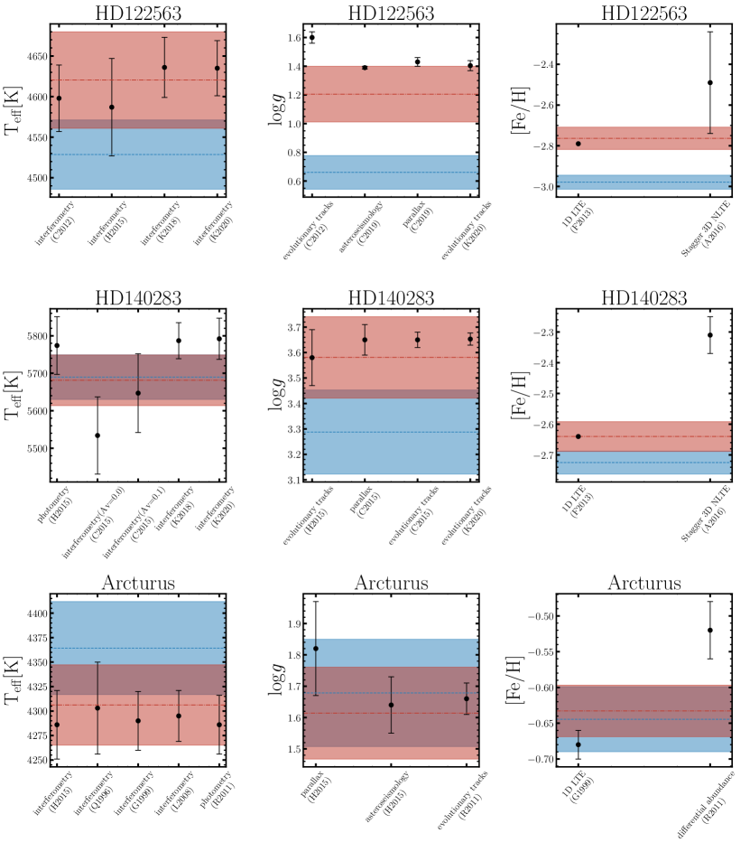
Figure 6: Comparison of our derived stellar parameters, $T_{\rm eff}$, $\log g$ and [Fe/H] using LOTUS to reference literature values derived non-spectroscopically (for $T_{\rm eff}$ and $\log g$) for HD122564, HD140283 and Arcturus. The mean NLTE values (red dashed lines) with their 1$\sigma$ confidence intervals (red shadow areas) and our mean LTE values (blue dashed lines) with their 1$\sigma$ confidence intervals (blue shadow areas), compared to to reference stellar parameters (black dots with error bars) for references on the x-axis. References are as follows: Q1996…Quirrenbach et al. (1996); G1999…Griffin & Lynas-Gray (1999); L2008…Lacour et al. (2008);R2011…Ramírez & Allende Prieto (2011);C2012…Creevey et al. (2012);F2013…Frebel et al. (2013);H2015…Heiter et al. (2015);C2015…Creevey et al. (2015);A2016…Amarsi et al. (2016);K2018…Karovicova et al. (2018);C2019…Creevey et al. (2019);K2020…Karovicova et al. (2020).

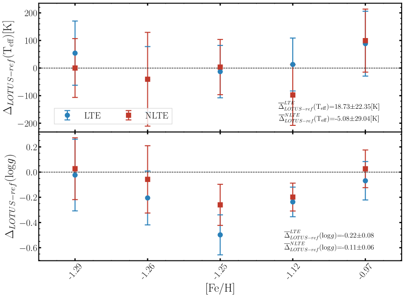
Figure 7: Differences in $\log g$ and $T_{\rm eff}$ between values derived using LOTUS versus reference values from Hawkins et al. (2016) for five GES metal-poor stars in their sample. Blue circles are LTE differences, while red squares are NLTE. Dashed lines in both panels are the zero baselines. Average systematic offsets are included in the text of each panel.

.

3.1 HD122563, HD140283, and Arcturus

The two metal-poor standard stars HD122563, HD140283 and the benchmark giant Arcturus have been widely analyzed independently in the literature. Their stellar parameters have therefore been derived spectroscopically (using 1D, 3D, LTE and NLTE assumptions, or a combination of each), as well as using non-spectroscopic methods and fundamental equations (e.g., using photometric calibrations, asteroseismology, or interferometric angular diameters). All three stars are dubbed benchmark stars which have been selected as comparison standards for the largest stellar surveys, especially in the $Gaia$-ESO spectroscopic survey (Jofré et al., 2014; Heiter et al., 2015). We adopt EW measurements of each benchmark star from literature publications as follows: HD122563 (Frebel et al., 2013), HD140283 (Frebel et al., 2013), Arcturus (Jofré et al., 2014). Frebel et al. (2013) measured their EW from high-resolution spectroscopic observations ($R\sim$35,000 in the blue and $\sim$28,000 in the red) of HD122563 and HD140283, obtained with the MIKE spectrograph (Bernstein et al., 2003) on the Magellan-Clay telescope at Las Campanas. A $R\geq$70,000 spectrum was used to derive EW for Arcturus from the VLT spectrum (Jofré et al., 2014). We derive the stellar parameters of each star and their uncertainties using LOTUS. We then compare our NLTE and LTE parameters with several independent determinations from the literature, as shown in Figure 6.

HD122563

We derive $T_{\rm eff}$ = 4620$\pm$59 K, $\log g$ = 1.21$\pm$0.19, $v_{\mathrm{mic}}$ = 1.89$\pm 0.06$ km s^-1 and [Fe/H] = $-$2.76$\pm$0.05 in NLTE, and $T_{\rm eff}$ = 4528$\pm$42 K , $\log g$ = 0.66$\pm$0.12, $v_{\mathrm{mic}}$ = 1.84$\pm 0.03$ km s^-1 and [Fe/H] = $-$2.98$\pm$0.03. Creevey et al. (2012) derived $T_{\rm eff}$ = 4598$\pm$41 K using an angular diameter observed with CHARA interferometry and Palomar interferometeric observations. Heiter et al. (2015) derived $T_{\rm eff}$ = 4587$\pm$60 K based on the angular diameters and bolometric fluxe calibrations, and $\log g$ = 1.44$\pm$0.24 from fitting evolutionary tracks. Karovicova et al. (2018) updated CHARA interferometry with more data and derived an effective temperature of $T_{\rm eff}$ = 4636$\pm$37 K. Later in Karovicova et al. (2020), they updated their data reduction pipeline and derived a new $T_{\rm eff}$ = 4635$\pm$34 K. Our NLTE $T_{\rm eff}$ derived for HD122563 agrees very well with $T_{\rm eff}$ determined in these studies using interferometric angular diameters, within $\sim$30 K, while the LTE $T_{\rm eff}$ deviated by $\sim 100$ K from the reference values.

And for $\log g$  results from the recent updated asteroseismic analysis are in agreement with the NLTE values in our work, which is close to the upper limit of 1$\sigma$ confidence interval.

For $\log g$, Creevey et al. (2012) used evolutionary track models to derive $\log g$ = 1.60$\pm$0.04 for HD122563, while Creevey et al. (2019) utilized the Hertzsprung telescope (SONG network node) to accurately measure the surface gravity of HD122563 using asteroseismology for the first time, and derived $\log g$ = 1.39$\pm$0.01. In their paper they also compare to $Gaia$ DR2 parallax-based $\log g$ = 1.43$\pm$0.03, which shows high consistency between these methods. Karovicova et al. (2020) also used evolutionary track models to derive $\log g$ = 1.404$\pm$0.03 for the same star. Our LOTUS $\log g$ = 1.22 in NLTE matches within $\sim 0.1$ dex the asteroseismic and parallax $\log g$ in Creevey et al. (2019), whereas the LTE value is 0.6 dex lower. This gives us strong confidence in LOTUS’ ability to derive NLTE surface gravities from spectroscopic observations.

We then compare our NLTE and LTE [Fe/H]  with those derived by Frebel et al. (2013) in 1D, LTE and Amarsi et al. (2016) in 3D,NLTE. Our NLTE [Fe/H] agrees with that determined in both studies within error bars, although Amarsi et al. (2016) derived a higher [Fe/H] = $-2.5$, which is likely due to considering 3D effects in their study.

HD140283

We derive $T_{\rm eff}$ = 5681$\pm$67 K , $\log g$ = 3.58$\pm$0.16, $v_{\mathrm{mic}}$ = 2.17$\pm$0.16 km s^-1 and [Fe/H] = $-2.64\pm$0.05 in NLTE, and $T_{\rm eff}$ = 5689$\pm$59 K , $\log g$ = 3.29$\pm$0.17, $v_{\mathrm{mic}}$ = 2.09$\pm$0.14 km s^-1 and [Fe/H] = $-2.72\pm$0.04 in LTE. Heiter et al. (2015) derived a mean $T_{\rm eff}$ = 5774$\pm$77 K for the sub-giant in their $Gaia$-ESO benchmark sample from photometric calibrations. Additionally, Creevey et al. (2015) used the VEGA interferometer on CHARA to determine $T_{\rm eff}$ = 5534$\pm$103 K (using $A_{V}$ = 0.0 mag) and $T_{\rm eff}$ =5 647$\pm$105 K (using $A_{V}$ = 0.1 mag). Karovicova et al. (2018) similarly derived an updated $T_{\rm eff}$ = 5787$\pm$48 K from additional interferometric data points, and afterwards updating their values to 5792$\pm$55 K in Karovicova et al. (2020). Our LTE and NLTE $T_{\rm eff}$ for HD140283 agree with the interferometric values derived in Creevey et al. (2015) within 120 K and Karovicova et al. (2018, 2020) within 80 K.

Heiter et al. (2015) derived $\log g$ = 3.58$\pm$0.11 using fundamental relations and adopting independently derived parallax for the star. Creevey et al. (2015) also derived a mean $\log g$ = 3.69$\pm$0.03, similarly from a combination of parallax and evolutionary track models. Both $\log g$ determined by parallax methods in Heiter et al. (2015) and Creevey et al. (2015) agree well with our NLTE value to within 0.05 dex. Karovicova et al. (2020) derived $\log g$ = 3.65$\pm$0.0 from evolutionary models. Our LTE values is, unexpectedly, 0.3 dex lower.

Similar to HD122563, we compare our [Fe/H] with 1D,LTE and 3D,NLTE abundances in Frebel et al. (2013) and Amarsi et al. (2016), respectively. Given that both studies derived their abundances by fixing $T_{\rm eff}$ and $\log g$, while ours were derived simultaneously using the global optimization method adopted in LOTUS, we warrant serious direct comparison with their values. Nevertheless, our NLTE values agree very well with that derived in Frebel et al. (2013) within 1$\sigma$, whereas is 0.3 dex lower as compared to Amarsi et al. (2016).

Arcturus

We derive $T_{\rm eff}$ = 4306$\pm$41 K, $\log g$ = 1.61$\pm$0.15, $v_{\mathrm{mic}}$ = 1.79$\pm$0.02 km s^-1 and [Fe/H] = $-0.63\pm$0.04 in NLTE, and $T_{\rm eff}$  = 4364$\pm$47 K , $\log g$ = 1.68$\pm$0.17 , $v_{\mathrm{mic}}$ = 1.76$\pm$0.02 km s^-1 and [Fe/H] = $-0.64\pm$0.05 in LTE. For $T_{\rm eff}$  Quirrenbach et al. (1996) used the MkIII Optical Interferometer on Mt. Wilson to determine Arcturus’ angular diameter and derived $T_{\rm eff}$ = 4303$\pm$47 K. Griffin & Lynas-Gray (1999) collected all literature results of interferometry observation up to their study and derived $T_{\rm eff}$ = 4290$\pm$30 K. Lacour et al. (2008) used the IOTA 3 telescope interferometer in the H band to derive $T_{\rm eff}$ = 4295$\pm$26 K. Additionally, Ramírez & Allende Prieto (2011) fit theoretical spectral energy distributions (SED) from visible blue bands to mid-infrared to derive $T_{\rm eff}$ = 4286$\pm$30 K. Finally, Heiter et al. (2015) derived a mean of 4274$\pm$83 K from different interferometric measurements, even though they warranted against using Arcturus as a benchmark given the large dispersion they obtained. All interferometric $T_{\rm eff}$ agree very well with our NLTE $T_{\rm eff}$ to within $\sim 20$ K. Our LTE value is, however, $\sim 80$ K higher.

Ramírez & Allende Prieto (2011) derived $\log g$ = 1.66$\pm$0.05 from HIPPARCOS parallax and isocrhone fitting, while Heiter et al. (2015) derived a fundamental $\log g$ = 1.64$\pm$0.09 based on seismic mass and $\log g$ = 1.82$\pm$0.15 from a compilation of parallax-based measurements. Our NLTE $\log g$ agrees very well with both results, whereas our LTE values is $0.1$ dex higher.

Griffin & Lynas-Gray (1999) derived [Fe/H] = $-0.68\pm$0.02 by comparing theoretical 1D, LTE SEDs with observed flux. Ramírez & Allende Prieto (2011) used a differential abundance analysis relative to the solar spectrum to derive [Fe/H] = $-0.52\pm$0.04. Our NLTE and LTE [Fe/H] are within 0.05 dex from each other, and agree well with the values derived in Griffin & Lynas-Gray (1999) while being $\sim 0.1$ dex as compared to differential abundance analysis in Ramírez & Allende Prieto (2011).

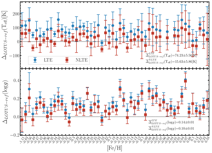
Figure 8: Same as in Figure 7 for the GES-K2 sample stars from Worley et al. (2020).

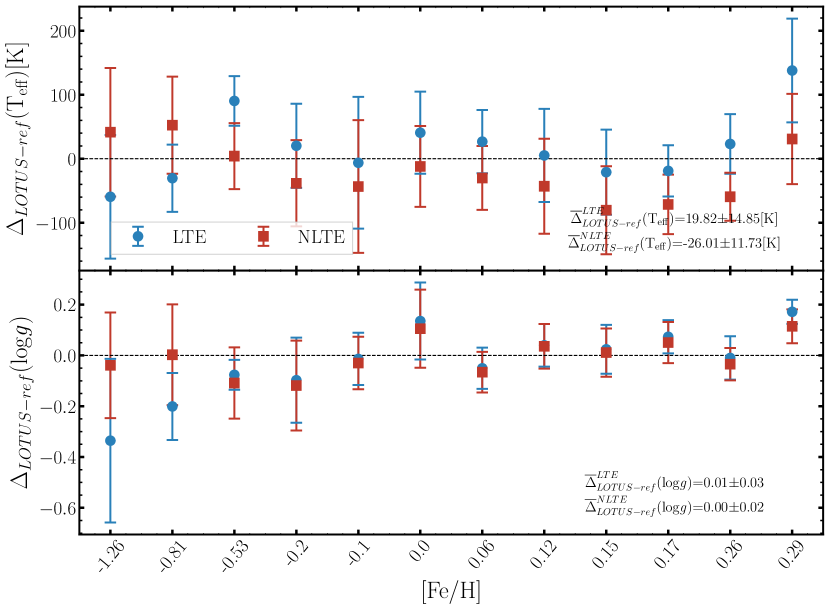
Figure 9: Same as in Figure 7 for the CHARA sample stars from Karovicova et al. (2020, 2021a, 2021b).

3.2 GES Metal-Poor Stars

We also test LOTUS on five metal-poor benchmark stars proposed by Hawkins et al. (2016) from the $Gaia$-ESO survey (GES). They determined $T_{\rm eff}$ via the Infrared Flux Method (IRFM) (Casagrande et al., 2011) using multi-band photometry and $\log g$ by fitting to evolutionary stellar models. The Fe i and Fe ii EWs for the sample stars were adopted from Hawkins et al. (2016), who used different EW measurements from different pipelines from the GES survey to derive their parameters. We use their EPINARBO (EPI) EWs derived with the FAMA pipeline following Magrini et al. (2013), as those were derived consistently. We compare our derived $T_{\rm eff}$ and $\log g$ using LOTUS to those in Hawkins et al. (2016) using the same Fe i and Fe ii lines. We find that our NLTE parameters are on average within $5\pm 29$ K from their $T_{\rm eff}$ and $0.11\pm 0.06$ for $\log g$ on average, whereas our LTE parameters are within $18\pm 22$ K and $0.22\pm 0.08$ dex for $T_{\rm eff}$ and $\log g$ respectively. Star by star comparisons are shown in Figure 7. Our NLTE parameters agree better with the non-spectroscopic parameters from Hawkins et al. (2016), as compared to LTE.

A larger $\log g$ dispersion is obtained for HD106038 though with [Fe/H]=$-1.25$ of $-0.25$ and $-0.45$, for both our NLTE and LTE results, respectively. With a 3D, Non-LTE analysis, and $Gaia$ EDR3 parallax, Giribaldi et al. (2021) derived $\log g$=4.29$\pm 0.04$, which is in excellent with our NLTE $\log g$=4.29$\pm$0.08. Additionally, only 35 Fe i lines used by Hawkins et al. (2016) were used to derive the stellar parameters in LOTUS  which decreases the accuracy of optimal values (see Section 5 for more details).

3.3 GES-K2 Stars

We also test LOTUS by deriving atmospheric stellar parameters of a sample of Kepler-2 (K2) star sample, which was also observed using a high-resolution UVES spectrograph on the VLT as part of the GES survey. Worley et al. (2020) combined the high-resolution spectroscopic observations from UVES, photometry, and precise asteroseismic data from K2 to derive self-consistent stellar parameters for these stars, which represent a good non-spectroscopic sample to compare our stellar parameters derived with LOTUS to.

We adopt the EW measurements from Worley et al. (2020) derived from high-resolution UVES spectroscopic observations. We chose a total of 52 stars from their sample. The majority of the stars in the sample are metal-rich with [Fe/H]$>-0.5$. Only six stars have [Fe/H]$<-0.5$. Worley et al. (2020) used the IRFM to determine photometrically calibrated $T_{\rm eff}$ for all their stars following Casagrande et al. (2010, 2011).

The average uncertainties reported in Worley et al. (2020) for $T_{\rm eff}$ and $\log g$ of the GES-K2 stars are $\pm 65$ K and $\pm 0.02$, respectively. We note that these values are close to our parameter grid resolution. We derive the stellar parameters for the 52 GES-K2 stars using LOTUS. Our results for $\log g$ and $T_{\rm eff}$ as compared to Worley et al. (2020) are shown in Figure 8 as a function of [Fe/H]. We find that the average differences between the LOTUS parameters are $\bar{\Delta}$$T_{\rm eff}$ = 74$\pm$6 K and $\bar{\Delta}$$\log g$ = 0.14$\pm$0.01 in LTE, and $\bar{\Delta}$$T_{\rm eff}$ = 16$\pm$6 K, $\bar{\Delta}$$\log g$ = 0.10$\pm$0.01 in NLTE. Both LTE and NLTE parameters agree well with the photometric and asteroseismic parameters from Worley et al. (2020) within their error bars, however our NLTE parameter derivations agree better for both $T_{\rm eff}$ and, particularly for $\log g$.

3.4 CHARA Interferometry Stars

Finally, we apply and test LOTUS on a sample of stars with effective temperatures derived homogeneously from interferometric angular diameters observed by CHARA from Karovicova et al. (2020, 2021a, 2021b). Karovicova et al. (2020) presented a study of interferometric observations of ten late-type metal-poor dwarfs and giants, whereas Karovicova et al. (2021a, b) showed a similar analysis for several metal-rich stars. For three of their stars (namely, HD122563, HD140283, and HD175305), we have already presented their analysis in Section 3.1 and 3.2. We, therefore, do not include the analysis of these stars again in this section. EW measurements of the total 12 stars were adopted from different literature sources including Takeda et al. (2005); Morel et al. (2014); Heiter et al. (2015); Takeda & Tajitsu (2015); Liu et al. (2020). The average uncertainties of the interferometric $T_{\rm eff}$ estimated by Karovicova et al. (2020, 2021a, 2021b) are within 1$\%$. The authors derived their $\log g$ values by fitting Dartmouth isochrones (Dotter et al., 2008) to their interferometric $T_{\rm eff}$. They thus derive median uncertainties for $\log g$ of 0.09 for their metal-poor star sample, 0.05 for their dwarf sample, and 0.07 for the giants/subgiants sample.

We find that on average the differences in $T_{\rm eff}$ and $\log g$ between the reference values (Karovicova et al., 2020, 2021a, 2021b) and those derived with LOTUS are within 26 K and 0.01 in NLTE, respectively. The NLTE parameters derived for all the stars agree within 1$\sigma$ as compared to the reference values, except for the $\log g$ value of HD121370 with [Fe/H]=0.29, which deviated by 0.12 for LTE and 0.18 for NLTE. Heiter et al. (2015), however, reported a seismic $\log g$ for this star of 3.83$\pm$0.02 dex, which agrees very with our NLTE result of 3.91$\pm$0.06 within 1$\sigma$.

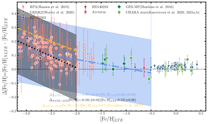
Figure 10: NLTE corrections $\Delta$[Fe/H] versus [Fe/H]_LTE determined for this work’s star sample using LOTUS. Different markers indicate stars from different studies as indicated. The Yellow dashed line is a linear fit from Ezzeddine et al. (2017) for stars with [Fe/H]$<$-4.0. The Blue dot-dash line is our fit to the stars for [Fe/H]$<-0.5$, and the black dotted line is our fit to the stars with [Fe/H]$<-2.0$.

4 NLTE corrections

The stars presented in Section 3 for testing LOTUS on benchmark stars with $T_{\rm eff}$ and $\log g$ derived using non-spectroscopic methods cover a limited range of metallicities (mostly with [Fe/H]$>-1.0$), as well as mainly dwarfs and sub-giant stars. However, NLTE stellar parameter “corrections” (also known as NLTE effects, defined as $\Delta$ NLTE = parameter(NLTE) - parameter(LTE)) have been shown in the literature to be more significant and important for evolved (giants and supergiant) metal-poor stars Lind et al. (2012); Ezzeddine et al. (2017). Thus, to be able to test our derived NLTE “corrections” on a larger, more metal-poor sample of giant stars, we derive LTE and NLTE stellar parameters for the $R$-process Alliance giant metal-poor star sample from Hansen et al. (2018), who derived the stellar parameters of 107 metal-poor stars ([Fe/H]$<-1.0$) selected based on their $r$-process enhancement from several surveys. The EW measurements for Fe i and Fe ii lines were adopted from Hansen et al. (2018), measured from their du Pont spectroscopic observations. We thus add the RPA sample stars to our test sample stars presented in Section 3, resulting in a significant sample covering a wide representative range of stellar parameters from $T_{\rm eff}$=4000 to 6500 K, $\log g$=0.0 to 4.5, and [Fe/H]=$-3.0$ to $-0.5$. The derived stellar parameters for the RPA stars, in LTE and NLTE, are also listed in Table 3.

We derive the NLTE corrections for [Fe/H] (denoted as $\Delta$[Fe/H]) for the full sample of stars. We plot the results as a function of [Fe/H]_LTE in Figure 10. As expected, $\Delta$[Fe/H] increases toward lower metallicities. Such effects have been shown in multiple previous studies as well (for e.g., Mashonkina et al., 2011; Lind et al., 2012; Bergemann et al., 2012; Amarsi et al., 2016; Ezzeddine et al., 2017). Ezzeddine et al. (2017) derived a linear relation between the NLTE correction for [Fe/H], $\Delta$[Fe/H], and [Fe/H](LTE) from 20 ultra metal-poor stars with [Fe/H]$<-4.0$, such as:

$$\Delta\mathrm{[Fe/H]}=-0.14\mathrm{[Fe/H]}_{\mathrm{LTE}}-0.15$$ (8)

They found that their relationship can also be extended for metal-poor benchmark stars at $-4.0<$ [Fe/H] $<-2.0$. It is therefore useful to re-derive this equation using our full stellar sample analyzed uniformly using LOTUS, for comparison. Following Ezzeddine et al. (2017), we re-derive the relation between $\Delta$[Fe/H] and [Fe/H](LTE) using our sample of stars . We re-derive the relation by (i) choosing only the stars with [Fe/H](LTE)$<-0.5$, and (ii) using the stars with [Fe/H](LTE)$<-2.0$. We thus derive $\Delta$[Fe/H]=

$$\begin{cases}-0.06(\pm 0.01)\mathrm{[Fe/H]}_{\mathrm{LTE}}-0.06(\pm 0.02),&\\ \mathrm{for~{}[Fe/H]}_{\mathrm{LTE}}<-0.5\\ -0.16(\pm 0.02)\mathrm{[Fe/H]}_{\mathrm{LTE}}-0.32(\pm 0.06),&\\ \mathrm{for~{}[Fe/H]}_{\mathrm{LTE}}<-2.0&\end{cases}$$ (9)

The two relations from these equations for $\Delta$[Fe/H], as well as that derived in Ezzeddine et al. (2017), are shown in Figure 10, fit to our test sample stars from Section 3 as well as the RPA sample. We find that even though the three relations agree within uncertainties (colored bands in Figure 10), they can, however, yield slightly different NLTE corrections depending on the metallicity range for which they were fit. For e.g., our relation derived using stars with [Fe/H]$<-2.0$ underestimates the NLTE [Fe/H] correction as compared to Ezzeddine et al. (2017) by $\sim 0.1$ dex at [Fe/H] = $-2.0$, while using the relation derived with [Fe/H]$<-0.5$ can underestimate the NLTE correction up to 0.2 dex. This demonstrates that while these relations can provide useful first-order estimates of the NLTE corrections, a complete NLTE analysis (e.g., using LOTUS) is needed for precise estimation of the corrections, as the former can be dependent on the incomplete sample of stars or metallicity range.

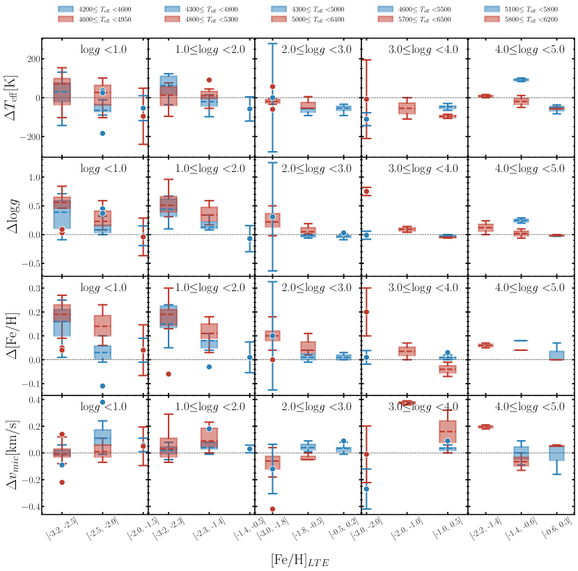
Figure 11: Box plots showing the NLTE corrections of stars considered in this work for stellar parameter $T_{\rm eff}$, $\log g$, [Fe/H], and $v_{\mathrm{mic}}$ as derived using LOTUS. Box plots are color-coded for two ranges of $T_{\rm eff}$for each $\log g$range, indicated at the top of each column. For intervals with only one star from our sample, boxes are replaced with dots and their error bars.

Similarly, we derive $\Delta$NLTE corrections for $T_{\rm eff}$, $\log g$, and $v_{\mathrm{mic}}$ for our sample stars. Again, we define the NLTE correction for $T_{\rm eff}$ as $\Delta$$T_{\rm eff}$ = $T_{\rm eff}$(NLTE) - $T_{\rm eff}$(LTE), for $\log g$ as $\Delta$$\log g$ = $\log g$(NLTE) - $\log g$(LTE), and for $v_{\mathrm{mic}}$ as $\Delta$$v_{\mathrm{mic}}$ = $v_{\mathrm{mic}}$(NLTE) - $v_{\mathrm{mic}}$(LTE). To best represent these corrections as a function of the other stellar parameters, we divide our sample into box plots grouped into different $T_{\rm eff}$ and $\log g$ bins, as a function of [Fe/H] on the x-axis. The results are shown in Figure 11.

In what follows we discuss the NLTE corrections we obtained for each parameter as a function of the other parameters, namely $T_{\rm eff}$, $\log g$  and [Fe/H]. We also compare our result to the theoretical NLTE stellar parameter corrections derived by Lind et al. (2012). We note, however, that our comparisons are affected by the fact that our analyzed stars do not cover exactly the same parameter space as theirs, and that our stellar parameters have been derived by LOTUS simultaneously, i.e., taking into account their inter-dependencies, as explained in details in Section 2, whereas Lind et al. (2012) derived their $\Delta$ NLTE corrections for each parameter independently, by fixing all the others. As shown in Figure 11, we find that the $T_{\rm eff}$ derived in NLTE are generally higher than those in LTE for very metal-poor ([Fe/H]$<-2.5$) super-giants and giant stars ($\log g$$<2.0$), with NLTE corrections up to 100 K, whereas lower $T_{\rm eff}$ are obtained in NLTE as compared to LTE as $\log g$ and [Fe/H] increases. Lind et al. (2012), who derived their $T_{\rm eff}$ using both excitation and ionization equilibrium by fixing gravity and other stellar parameters in the process. Similarly, they also restrict their Fe i line transitions to certain cutoffs, choosing only lines with EP$>3.5$ eV. They found that their ionization $\Delta$$T_{\rm eff}$ yielded lower LTE $T_{\rm eff}$ as compared to NLTE (see their Figure 5), whereas their excitation $\Delta$$T_{\rm eff}$ yielded negligible positive corrections for $T_{\rm eff}$$<4500$. More pronounced negative corrections were obtained for horizontal branches, supergiants, and extremely metal-poor stars, which are not covered in our sample stars. As noted above, our derived $T_{\rm eff}$ using LOTUS implement the contribution from both excitation and ionization equilibrium, by taking into account their $T_{\rm eff}$-$\log g$ inter-dependencies. In that context, a thorough comparison of our $\Delta$$T_{\rm eff}$ results to either excitation or ionization theoretical corrections derived by Lind et al. (2012) are not very useful, however, similar to their results we generally find that the NLTE corrections for the bulk of our stars are affected by less than 50 K (and up to 100 K) in the considered parameter range, which is within our derived uncertainties.

We also derive $\Delta$$\log g$ for our sample stars. As expected, the NLTE corrections for $\log g$ increase towards lower gravities, lower metallicities, and higher temperatures. On average, our corrections are $\sim+0.3-0.5$ for [Fe/H]$<-2.0$, $\sim+0.1-0.3$ for $-2.0<$[Fe/H]$<-1.0$, for giants and supergiant stars with $\log g$$<2.0$, with outliers reaching up to 1.0 dex. For stars with $\log g$$>2.0$, the NLTE corrections can be up to $\sim$0.3 depending on metallicities. These results broadly agree with the theoretical corrections derived in Lind et al. (2012). It can thus be concluded that LTE analyses can strongly underestimate the surface gravities of stars, particularly for warmer metal-poor giants, and should thus be reliably derived in NLTE for reliable consequent stellar population analyses.

Finally, the NLTE corrections for $v_{\mathrm{mic}}$ are generally small and are within $2.0$ km s^-1 from those derived in LTE. The corrections are mainly positive for lower metallicity giants and supergiant stars, as in particular their Fe i lines are more strongly affected by NLTE, which leads to lower microturbulent velocities in LTE as compared to NLTE. Our results are generally consistent with the $\Delta$$v_{\mathrm{mic}}$ derived by Lind et al. (2012) from their theoretical models.

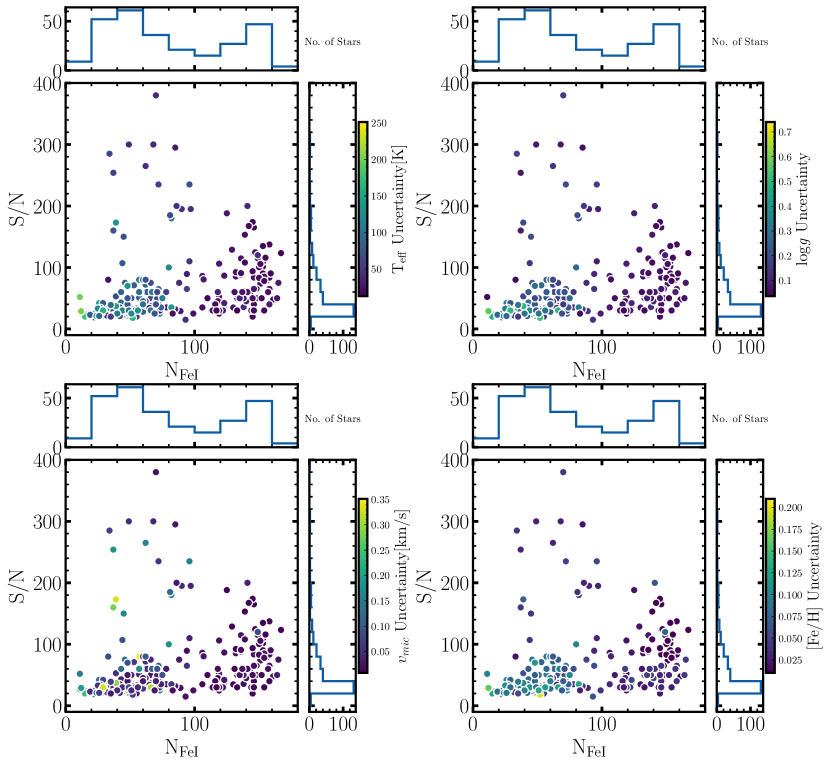
Figure 12: Derived stellar parameter uncertainties as a functions of the number of Fe I lines and S/N ratios in our sample of stars from Section 4, in addition to metal-poor stars with high S/N from Ezzeddine et al. (2020).

5 Caveats

We have so far described and demonstrated that LOTUS can be used as a reliable tool to derive NLTE and LTE atmospheric stellar parameters. There are, however, some caveats that warrant pointing out which can affect the results, particularly for stars occupying certain parameter spaces in our grids.

EW Interpolation

A key component of LOTUS is its interpolation module that expresses the EW as a function of stellar parameters, using the generalized curve of growth (GCOG). As explained in Section 2.3.1, we conduct thorough tests to choose the best polynomial interpolator for each spectral type. However, we find that some models are not adequate to reliably fit the GCOG, particularly for parameter regions where EW variations have smaller dependencies on stellar parameters. This is demonstrated in Figure 2, where the EW of the Fe i line at 4077 Å varies less strongly with $v_{\mathrm{mic}}$ at higher $T_{\rm eff}$ and lower $\log g$. Thus, the iron abundances derived from these interpolated models can deviate up to 0.5 dex in abundances from those computed directly from MULTI2.3 output (i.e, non interpolated EWs). Such large offsets are likely due to lower than optimal orders of polynomials chosen for some spectral types in these parameter regions (see Section 2.3.1 for details), where the EW of those lines not being sensitive to the variation of atmospheric stellar parameters, or being too small (close to zero) at most atmospheric stellar parameters. We emphasize though, that the number of such lines is limited and should not impact the statistical properties of the interpolation performance for the lines considered in our linelist, as shown in Figure 3.

Number of Fe I lines and S/N ratios

The derived atmospheric stellar parameters could be affected by the number of Fe i and Fe ii lines utilized in the parameter optimization in LOTUS. We, therefore, investigate the derived uncertainties of the stellar parameters using LOTUS as a function of the number of Fe I lines and the S/N ratio as shown in Figure 12. To demonstrate our results over a representative statistical sample of stars covering a wide range of S/N ratios, we use the full star sample from Section 4, supplemented by metal-poor stars from Ezzeddine et al. (2020) which cover higher S/N values (S/N$>$100) than those in Hansen et al. (2018). We can see in Figure 12 that the uncertainties derived for each stellar parameter as a function of the number of Fe i and S/N ratio decrease as a function of increasing the number of Fe i and increasing the S/N ratio. For stars with $N_{\mathrm{lines}}>100$ or stars with $N_{\mathrm{lines}}<100$ and S/N$>$100, the uncertainty are $<50$ K for $T_{\rm eff}$, $<0.1$ dex for $\log g$, $<0.05$ dex for [Fe/H] and $<0.02$ km s^-1 for $v_{\mathrm{mic}}$. For stars with $N_{\mathrm{lines}}<100$ and S/N$<$60, however, the uncertainties can reach up to 200 K for $T_{\rm eff}$, 0.5 dex for $\log g$, 0.3 dex for [Fe/H] and 0.2 km s^-1 for $v_{\mathrm{mic}}$. It is notable to mention, though, that higher uncertainties are more strongly correlated to lower S/N ($<40$). We thus recommend that users try to utilize ”good-quality” EW measurements for their Fe i (and Fe ii) lines to obtain reliable results and smaller uncertainty derivation in LOTUS. This is particularly useful if the number of measured EW lines for a star is too small ($<100$). Additionally, as the number of Fe ii lines usually detected in cool FGK stellar spectra can be smaller than the number of Fe i lines (on the order of 5-25 lines, depending on the [Fe/H] of the star), we moreover recommend that users try to maximize the number of Fe ii EW line measurements in the stars, if possible, to increase the precision of the parameter determination. In future work, we plan to test LOTUS on a sample of low resolution spectroscopic observations (as compared to high-resolution data for the same stars) to accurately quantify the effects of the spectral resolution on the results of the stellar parameters derived by LOTUS.

K-type stars

The atmospheric stellar parameters, particularly $\log g$, derived for K-type stars using LOTUS can have larger uncertainties than those derived for other spectral types. Tsantaki et al. (2019) noted that $\log g$ determined for K-type stars using ionization balance between Fe i and Fe ii lines are underestimated depending on the choice of Fe ii lines used in the optimization. We investigate this effect on our GES-K2 sample, in which most of the stars are K-type giants or sub-giants. We find that both our NLTE and LTE results can indeed overestimate the surface gravities up to 0.1 dex as compared to asteroseismic values, depending on the selection of Fe ii lines.

3D models

Since our atmospheric stellar models are limited to 1D, our determined iron abundances might suffer from 3D effects due to atmospheric inhomogeneities, horizontal radiation transfer, as well as the differences in the mean temperature stratification Amarsi et al. (2016) between 1D and 3D models. The latter can lead to underestimated abundances derived from Fe i and Fe ii lines, on average up to $0.1$ dex in 1D, NLTE as compared with Fe abundances derived using 3D, NLTE. Such effects are, however, more strongly pronounced for Fe ii lines than Fe i as explained in Amarsi et al. (2016). We find that adding a $0.1$ dex correction for our 1D, NLTE [Fe/H] for HD122563 brings it closer to the 3D, NLTE [Fe/H] derived in (Amarsi et al., 2016).

On the other hand, we find that a difference of $0.2$ dex as compared to Amarsi et al. (2016) is still present when adding the same [Fe/H] correction for HD140283. This can be explained by the stellar parameter differences adopted in both studies, as well as the difference between linelists. However, as noted in Amarsi et al. (2016) and Amarsi et al. (2022), 3D corrections can nevertheless be smaller than the NLTE corrections determined for low metallicity evolved stars. Therefore, including 1D, NLTE corrections in the determination of Fe i and Fe ii lines can significantly improve the derived stellar parameters as compared to 1D, LTE.

6 Summary & Conclusions

We present the open-source code, LOTUS, developed to automatically derive fast and precise atmospheric stellar parameters ($T_{\rm eff}$, $\log g$, [Fe/H] and $v_{\mathrm{mic}}$) of stars in 1D, LTE, and 1D, NLTE using Fe i and Fe ii equivalent width measurement from stellar spectra.

LOTUS implements a generalized curve of growth (GCOG) interpolation to derive abundances from a pre-computed grid of theoretical NLTE EW in a high-resolution and dense spectral parameter space. The GCOG takes into account the EW dependencies on stellar atmospheric parameters. A global differential evolution optimization algorithm, tailored to the spectral type of the star, is then used to derive the fundamental stellar parameters. In addition, LOTUS can be used to estimate precise uncertainties for each stellar parameter using a well-tested Markov Chain Monte Carlo (MCMC) algorithm.

We tested our code on several benchmark stars and stellar samples with reliable non-spectroscopic (from asteroseismic, photometric, and interferometric observations) measurements for a wide range of parameter space typical for FGK stars. We find that our NLTE-derived stellar parameters for $T_{\rm eff}$ and $\log g$ are within 30 K and 0.1 dex for benchmark stars including the metal-poor standard stars, HD140283 and HD122563, as well as Arcturus. We also test LOTUS on a large sample of $Gaia$-ESO (GES) dwarf stars from Hawkins et al. (2016) and GES-K2 with asteroseismic gravities from K2, as well as stars with CHARA interferometric observations. Similarly, we find that LOTUS performs very well in reproducing the non-spectroscopic $T_{\rm eff}$ and $\log g$ on average within $<20$ K and $<0.1$ dex in NLTE, as compared to $\sim 70$ K and $\sim 0.2$ dex in LTE.

Moreover, we apply LOTUS on a large sample of metal-poor stars from the R-Process Alliance (RPA, Hansen et al. 2018). We use the RPA sample as well as the test sample stars to derive NLTE stellar parameter corrections for our stars and review the $\Delta$[Fe/H] versus [Fe/H](LTE) relation derived in Ezzeddine et al. (2017). We find that our NLTE corrections agree with theoretical corrections predicted by Lind et al. (2012), where general trends of corrections were found to increasing toward metal-poor evolved stars, as expected.

We test LOTUS thoroughly for its performance for different spectral types and parameter space. We find that despite some caveats discussed in Section 5, LOTUS can overall be reliably used to provide fast and accurate NLTE derivation for a wide range of stellar parameters, especially metal-poor giants which can be strongly affected by deviations from LTE. We thus strongly recommend that the community use it to apply for the spectroscopic analyses of stars and stellar populations.

We provide open community access to LOTUS, as well as the pre-computed interpolated LTE and NLTE EW grids available on Github github, with documentation and working examples on Readthedocs book.

Appendix A Linelist of Fe i and Fe ii in LOTUS

Table 2: Fe i and Fe ii linelist selected for LOTUS (see Section  2.1.4 for details)

Species	$\lambda$($\AA$)	Elow(ev)	loggf
Fe i	3440.61	0.00	$-$0.67
Fe i	3440.99	0.05	$-$0.96
Fe i	3447.28	2.20	$-$1.02
Fe i	3450.33	2.22	$-$0.90
Fe i	3451.91	2.22	$-$1.00
Fe i	3476.70	0.12	$-$1.51
Fe i	3490.57	0.05	$-$1.10
Fe i	3497.84	0.11	$-$1.55
Fe i	3540.12	2.87	$-$0.71
Fe i	3565.38	0.96	$-$0.13
Fe i	3608.86	1.01	$-$0.10
Fe i	3618.77	0.99	$-$0.00
Fe i	3647.84	0.92	$-$0.19
Fe i	3689.46	2.94	$-$0.17
Fe i	3719.93	0.00	$-$0.43
Fe i	3727.62	0.96	$-$0.63
Fe i	3742.62	2.94	$-$0.81
Fe i	3758.23	0.96	$-$0.03
Fe i	3763.79	0.99	$-$0.24
Fe i	3765.54	3.24	0.48
Fe i	3786.68	1.01	$-$2.22
Fe i	3787.88	1.01	$-$0.86
Fe i	3805.34	3.30	0.31
Fe i	3808.73	2.56	$-$1.17
Fe i	3815.84	1.48	0.23
Fe i	3820.43	0.86	0.12
Fe i	3825.88	0.91	$-$0.04
Fe i	3827.82	1.56	0.06
Fe i	3840.44	0.99	$-$0.51
Fe i	3841.05	1.61	$-$0.04
Fe i	3849.97	1.01	$-$0.87
Fe i	3856.37	0.05	$-$1.29
Fe i	3865.52	1.01	$-$0.98
Fe i	3878.02	0.96	$-$0.91
Fe i	3895.66	0.11	$-$1.67
Fe i	3899.71	0.09	$-$1.53
Fe i	3902.95	1.56	$-$0.47
Fe i	3920.26	0.12	$-$1.75
Fe i	3922.91	0.05	$-$1.65
Fe i	3949.95	2.18	$-$1.25
Fe i	3977.74	2.20	$-$1.12
Fe i	4005.24	1.56	$-$0.61
Fe i	4045.81	1.49	0.28
Fe i	4058.22	3.21	$-$1.18
Fe i	4063.59	1.56	0.06
Fe i	4067.98	3.21	$-$0.53
Fe i	4070.77	3.24	$-$0.87
Fe i	4071.74	1.61	$-$0.02
Fe i	4114.44	2.83	$-$1.30
Fe i	4132.06	1.61	$-$0.68
Fe i	4134.68	2.83	$-$0.65
Fe i	4143.87	1.56	$-$0.51
Fe i	4147.67	1.49	$-$2.10
Fe i	4150.25	3.43	$-$1.19
Fe i	4154.50	2.83	$-$0.69
Fe i	4156.80	2.83	$-$0.81
Fe i	4157.78	3.42	$-$0.40
Fe i	4158.79	3.43	$-$0.70
Fe i	4174.91	0.91	$-$2.97
Fe i	4175.64	2.85	$-$0.83
Fe i	4181.76	2.83	$-$0.37
Fe i	4182.38	3.02	$-$1.18
Fe i	4184.89	2.83	$-$0.87
Fe i	4187.04	2.45	$-$0.56
Fe i	4187.80	2.42	$-$0.55
Fe i	4191.43	2.47	$-$0.67
Fe i	4195.33	3.33	$-$0.49
Fe i	4199.10	3.05	0.16
Fe i	4202.03	1.49	$-$0.71
Fe i	4216.18	0.00	$-$3.36
Fe i	4217.55	3.43	$-$0.48
Fe i	4222.21	2.45	$-$0.97
Fe i	4227.43	3.33	0.27
Fe i	4233.60	2.48	$-$0.60
Fe i	4238.81	3.40	$-$0.23
Fe i	4250.12	2.47	$-$0.41
Fe i	4250.79	1.56	$-$0.71
Fe i	4260.47	2.40	0.08
Fe i	4271.15	2.45	$-$0.35
Fe i	4271.76	1.49	$-$0.16
Fe i	4282.40	2.18	$-$0.78
Fe i	4325.76	1.61	0.01
Fe i	4352.73	2.22	$-$1.29
Fe i	4375.93	0.00	$-$3.03
Fe i	4388.41	3.60	$-$0.68
Fe i	4404.75	1.56	$-$0.14
Fe i	4415.12	1.61	$-$0.62
Fe i	4427.31	0.05	$-$3.04
Fe i	4430.61	2.22	$-$1.66
Fe i	4432.57	3.57	$-$1.58
Fe i	4442.34	2.20	$-$1.25
Fe i	4443.19	2.86	$-$1.04
Fe i	4447.72	2.22	$-$1.36
Fe i	4461.65	0.09	$-$3.21
Fe i	4466.55	2.83	$-$0.60
Fe i	4484.22	3.60	$-$0.64
Fe i	4489.74	0.12	$-$3.97
Fe i	4494.56	2.20	$-$1.14
Fe i	4514.18	3.05	$-$1.96
Fe i	4531.15	1.48	$-$2.16
Fe i	4547.85	3.55	$-$0.82
Fe i	4574.22	3.21	$-$2.35
Fe i	4592.65	1.56	$-$2.45
Fe i	4595.36	3.30	$-$1.76
Fe i	4602.00	1.61	$-$3.15
Fe i	4602.94	1.49	$-$2.22
Fe i	4607.65	3.27	$-$1.33
Fe i	4619.29	3.60	$-$1.06
Fe i	4630.12	2.28	$-$2.58
Fe i	4637.50	3.28	$-$1.29
Fe i	4643.46	3.65	$-$1.15
Fe i	4647.43	2.95	$-$1.35
Fe i	4661.97	2.99	$-$2.50
Fe i	4668.13	3.27	$-$1.08
Fe i	4704.95	3.69	$-$1.32
Fe i	4733.59	1.49	$-$2.99
Fe i	4736.77	3.21	$-$0.67
Fe i	4786.81	3.02	$-$1.61
Fe i	4787.83	3.00	$-$2.62
Fe i	4788.76	3.24	$-$1.763
Fe i	4789.65	3.55	$-$0.96
Fe i	4793.96	3.05	$-$3.43
Fe i	4794.35	2.42	$-$3.95
Fe i	4800.65	4.14	$-$1.03
Fe i	4802.88	3.64	$-$1.51
Fe i	4807.71	3.37	$-$2.15
Fe i	4808.15	3.25	$-$2.69
Fe i	4869.46	3.55	$-$2.42
Fe i	4871.32	2.87	$-$0.34
Fe i	4872.14	2.88	$-$0.57
Fe i	4873.75	3.30	$-$2.96
Fe i	4875.88	3.33	$-$1.90
Fe i	4877.60	3.00	$-$3.05
Fe i	4882.14	3.42	$-$1.48
Fe i	4885.43	3.88	$-$0.97
Fe i	4890.76	2.88	$-$0.38
Fe i	4891.49	2.85	$-$0.11
Fe i	4896.44	3.88	$-$1.89
Fe i	4903.31	2.88	$-$0.89
Fe i	4905.13	3.93	$-$1.73
Fe i	4907.73	3.43	$-$1.70
Fe i	4910.02	3.40	$-$1.28
Fe i	4911.78	3.93	$-$1.75
Fe i	4918.99	2.86	$-$0.34
Fe i	4920.50	2.83	0.07
Fe i	4924.77	2.28	$-$2.11
Fe i	4938.81	2.88	$-$1.08
Fe i	4939.69	0.86	$-$3.34
Fe i	4946.39	3.37	$-$1.11
Fe i	4950.11	3.42	$-$1.49
Fe i	4962.57	4.18	$-$1.18
Fe i	4966.09	3.33	$-$0.79
Fe i	4969.92	4.22	$-$0.71
Fe i	4985.55	2.87	$-$1.33
Fe i	4992.79	4.26	$-$2.35
Fe i	4994.13	0.92	$-$3.08
Fe i	4999.11	4.19	$-$1.64
Fe i	5001.86	3.88	$-$0.01
Fe i	5002.79	3.40	$-$1.46
Fe i	5005.71	3.88	$-$0.12
Fe i	5006.12	2.83	$-$0.61
Fe i	5012.69	4.28	$-$1.69
Fe i	5014.94	3.94	$-$0.18
Fe i	5022.24	3.98	$-$0.33
Fe i	5023.19	4.28	$-$1.50
Fe i	5028.13	3.57	$-$1.02
Fe i	5039.25	3.37	$-$1.52
Fe i	5044.21	2.85	$-$2.02
Fe i	5048.44	3.96	$-$1.00
Fe i	5049.82	2.28	$-$1.35
Fe i	5051.63	0.92	$-$2.80
Fe i	5054.64	3.64	$-$1.92
Fe i	5058.50	3.64	$-$2.83
Fe i	5060.08	0.00	$-$5.43
Fe i	5068.77	2.94	$-$1.04
Fe i	5079.22	2.20	$-$2.07
Fe i	5079.74	0.99	$-$3.22
Fe i	5083.34	0.96	$-$2.96
Fe i	5088.15	4.15	$-$1.68
Fe i	5107.45	0.99	$-$3.09
Fe i	5107.64	1.56	$-$2.36
Fe i	5109.65	4.30	$-$0.98
Fe i	5115.78	3.57	$-$2.64
Fe i	5123.72	1.01	$-$3.07
Fe i	5127.36	0.92	$-$3.31
Fe i	5131.47	2.22	$-$2.52
Fe i	5133.69	4.18	0.36
Fe i	5141.74	2.42	$-$2.24
Fe i	5150.84	0.99	$-$3.04
Fe i	5151.91	1.01	$-$3.32
Fe i	5166.28	0.00	$-$4.20
Fe i	5171.60	1.49	$-$1.79
Fe i	5191.45	3.04	$-$0.55
Fe i	5192.34	3.00	$-$0.42
Fe i	5194.94	1.56	$-$2.09
Fe i	5197.94	4.30	$-$1.54
Fe i	5198.71	2.22	$-$2.13
Fe i	5202.34	2.18	$-$1.84
Fe i	5215.18	3.27	$-$0.86
Fe i	5216.27	1.61	$-$2.15
Fe i	5217.39	3.21	$-$1.07
Fe i	5223.18	3.63	$-$1.78
Fe i	5225.53	0.11	$-$4.79
Fe i	5228.38	4.22	$-$1.19
Fe i	5232.94	2.94	$-$0.06
Fe i	5242.49	3.63	$-$0.97
Fe i	5243.78	4.26	$-$1.05
Fe i	5247.05	0.09	$-$4.95
Fe i	5250.21	0.12	$-$4.93
Fe i	5250.65	2.20	$-$2.18
Fe i	5253.02	2.28	$-$3.84
Fe i	5253.46	3.28	$-$1.58
Fe i	5262.88	3.25	$-$2.56
Fe i	5263.31	3.27	$-$0.87
Fe i	5266.56	3.00	$-$0.39
Fe i	5281.79	3.04	$-$0.83
Fe i	5283.62	3.24	$-$0.52
Fe i	5285.13	4.43	$-$1.66
Fe i	5288.52	3.69	$-$1.49
Fe i	5293.96	4.14	$-$1.77
Fe i	5294.55	3.64	$-$2.76
Fe i	5295.31	4.42	$-$1.59
Fe i	5300.40	4.59	$-$1.65
Fe i	5302.30	3.28	$-$0.74
Fe i	5307.36	1.61	$-$2.99
Fe i	5321.11	4.43	$-$1.09
Fe i	5322.04	2.28	$-$2.80
Fe i	5324.18	3.21	$-$0.11
Fe i	5332.90	1.56	$-$2.78
Fe i	5339.93	3.27	$-$0.63
Fe i	5341.02	1.61	$-$1.95
Fe i	5364.87	4.45	0.23
Fe i	5365.40	3.57	$-$1.02
Fe i	5367.47	4.42	0.44
Fe i	5369.96	4.37	0.54
Fe i	5371.49	0.96	$-$1.64
Fe i	5373.71	4.47	$-$0.71
Fe i	5379.57	3.69	$-$1.42
Fe i	5383.37	4.31	0.65
Fe i	5386.33	4.15	$-$1.67
Fe i	5389.48	4.42	$-$0.41
Fe i	5395.22	4.45	$-$2.07
Fe i	5397.13	0.92	$-$1.99
Fe i	5398.28	4.45	$-$0.63
Fe i	5405.77	0.99	$-$1.85
Fe i	5410.91	4.47	0.4
Fe i	5412.78	4.43	$-$1.72
Fe i	5415.20	4.39	0.64
Fe i	5417.03	4.42	$-$1.58
Fe i	5424.07	4.32	0.52
Fe i	5429.70	0.96	$-$1.88
Fe i	5434.52	1.01	$-$2.12
Fe i	5436.59	2.28	$-$2.96
Fe i	5441.34	4.31	$-$1.63
Fe i	5445.04	4.39	$-$0.02
Fe i	5461.55	4.45	$-$1.8
Fe i	5464.28	4.14	$-$1.40
Fe i	5466.40	4.37	$-$0.63
Fe i	5470.09	4.45	$-$1.71
Fe i	5473.90	4.15	$-$0.72
Fe i	5483.10	4.15	$-$1.39
Fe i	5487.15	4.42	$-$1.43
Fe i	5491.83	4.19	$-$2.19
Fe i	5493.50	4.10	$-$1.48
Fe i	5494.46	4.08	$-$1.99
Fe i	5497.52	1.01	$-$2.85
Fe i	5501.47	0.96	$-$3.05
Fe i	5506.78	0.99	$-$2.80
Fe i	5522.45	4.21	$-$1.45
Fe i	5525.54	4.23	$-$1.08
Fe i	5536.58	2.83	$-$3.71
Fe i	5539.28	3.64	$-$2.56
Fe i	5543.94	4.22	$-$1.04
Fe i	5546.51	4.37	$-$1.21
Fe i	5552.69	4.95	$-$1.89
Fe i	5554.90	4.55	$-$0.27
Fe i	5560.21	4.43	$-$1.09
Fe i	5563.60	4.19	$-$0.75
Fe i	5569.62	3.42	$-$0.52
Fe i	5576.09	3.43	$-$0.90
Fe i	5586.76	3.37	$-$0.11
Fe i	5587.57	4.14	$-$1.75
Fe i	5618.63	4.21	$-$1.25
Fe i	5619.60	4.39	$-$1.60
Fe i	5624.02	4.39	$-$1.38
Fe i	5624.54	3.42	$-$0.76
Fe i	5633.95	4.99	$-$0.23
Fe i	5635.82	4.26	$-$1.79
Fe i	5636.70	3.64	$-$2.51
Fe i	5638.26	4.22	$-$0.72
Fe i	5641.43	4.26	$-$1.08
Fe i	5649.99	5.10	$-$0.82
Fe i	5651.47	4.47	$-$1.90
Fe i	5652.32	4.26	$-$1.85
Fe i	5653.87	4.39	$-$1.54
Fe i	5655.18	5.06	$-$0.60
Fe i	5661.35	4.28	$-$1.76
Fe i	5662.52	4.18	$-$0.41
Fe i	5667.52	4.18	$-$1.58
Fe i	5679.02	4.65	$-$0.82
Fe i	5686.53	4.55	$-$0.45
Fe i	5691.50	4.30	$-$1.45
Fe i	5696.09	4.55	$-$1.72
Fe i	5698.02	3.64	$-$2.58
Fe i	5701.54	2.56	$-$2.22
Fe i	5705.46	4.30	$-$1.35
Fe i	5731.76	4.26	$-$1.20
Fe i	5732.30	4.99	$-$1.46
Fe i	5741.85	4.26	$-$1.67
Fe i	5742.96	4.18	$-$2.41
Fe i	5753.12	4.26	$-$0.62
Fe i	5760.34	3.64	$-$2.39
Fe i	5775.08	4.22	$-$1.08
Fe i	5778.45	2.59	$-$3.43
Fe i	5784.66	3.40	$-$2.55
Fe i	5816.37	4.55	$-$0.60
Fe i	5835.10	4.26	$-$2.27
Fe i	5837.70	4.29	$-$2.24
Fe i	5838.37	3.94	$-$2.24
Fe i	5849.68	3.69	$-$2.89
Fe i	5853.15	1.49	$-$5.18
Fe i	5855.08	4.61	$-$1.48
Fe i	5858.78	4.22	$-$2.16
Fe i	5883.82	3.96	$-$1.26
Fe i	5902.47	4.59	$-$1.71
Fe i	5905.67	4.65	$-$0.69
Fe i	5916.25	2.45	$-$2.99
Fe i	5927.79	4.65	$-$0.99
Fe i	5929.68	4.55	$-$1.31
Fe i	5930.18	4.65	$-$0.23
Fe i	5934.65	3.93	$-$1.07
Fe i	5940.99	4.18	$-$2.05
Fe i	5956.69	0.86	$-$4.60
Fe i	6003.01	3.88	$-$1.10
Fe i	6008.56	3.88	$-$0.98
Fe i	6012.21	2.22	$-$4.04
Fe i	6024.06	4.55	$-$0.12
Fe i	6027.05	4.08	$-$1.09
Fe i	6056.00	4.73	$-$0.32
Fe i	6065.48	2.61	$-$1.53
Fe i	6079.01	4.65	$-$1.02
Fe i	6082.71	2.22	$-$3.58
Fe i	6093.64	4.61	$-$1.40
Fe i	6094.37	4.65	$-$1.84
Fe i	6096.66	3.98	$-$1.83
Fe i	6120.25	0.91	$-$5.97
Fe i	6127.91	4.14	$-$1.40
Fe i	6136.61	2.45	$-$1.40
Fe i	6136.99	2.20	$-$2.95
Fe i	6137.69	2.59	$-$1.40
Fe i	6151.62	2.18	$-$3.30
Fe i	6165.36	4.14	$-$1.47
Fe i	6173.33	2.22	$-$2.88
Fe i	6187.99	3.94	$-$1.62
Fe i	6191.56	2.43	$-$1.42
Fe i	6200.31	2.61	$-$2.43
Fe i	6213.43	2.22	$-$2.48
Fe i	6219.28	2.20	$-$2.43
Fe i	6226.73	3.88	$-$2.12
Fe i	6229.23	2.85	$-$2.81
Fe i	6230.72	2.56	$-$1.28
Fe i	6232.64	3.65	$-$1.24
Fe i	6240.65	2.22	$-$3.17
Fe i	6246.32	3.60	$-$0.77
Fe i	6252.56	2.40	$-$1.69
Fe i	6265.13	2.18	$-$2.55
Fe i	6270.22	2.86	$-$2.47
Fe i	6271.28	3.33	$-$2.70
Fe i	6297.79	2.22	$-$2.74
Fe i	6301.50	3.65	$-$0.71
Fe i	6315.81	4.08	$-$1.63
Fe i	6322.69	2.59	$-$2.43
Fe i	6330.85	4.73	$-$1.64
Fe i	6335.33	2.20	$-$2.18
Fe i	6336.82	3.69	$-$0.85
Fe i	6338.88	4.80	$-$0.96
Fe i	6344.15	2.43	$-$2.92
Fe i	6355.03	2.84	$-$2.29
Fe i	6364.36	4.80	$-$1.33
Fe i	6380.74	4.19	$-$1.38
Fe i	6393.60	2.43	$-$1.58
Fe i	6400.32	0.91	$-$4.32
Fe i	6408.02	3.69	$-$0.99
Fe i	6411.65	3.65	$-$0.59
Fe i	6421.35	2.28	$-$2.03
Fe i	6430.85	2.18	$-$2.01
Fe i	6475.62	2.56	$-$2.94
Fe i	6481.87	2.28	$-$2.98
Fe i	6494.98	2.40	$-$1.27
Fe i	6496.47	4.80	$-$0.53
Fe i	6498.94	0.96	$-$4.69
Fe i	6518.37	2.83	$-$2.44
Fe i	6533.93	4.56	$-$1.36
Fe i	6546.24	2.76	$-$1.54
Fe i	6569.21	4.73	$-$0.38
Fe i	6574.23	0.99	$-$5.00
Fe i	6592.91	2.73	$-$1.47
Fe i	6593.87	2.43	$-$2.42
Fe i	6597.56	4.80	$-$0.97
Fe i	6609.11	2.56	$-$2.69
Fe i	6627.54	4.55	$-$1.59
Fe i	6648.08	1.01	$-$5.92
Fe i	6677.99	2.69	$-$1.42
Fe i	6699.14	4.59	$-$2.10
Fe i	6703.57	2.76	$-$3.06
Fe i	6713.74	4.80	$-$1.50
Fe i	6733.15	4.64	$-$1.15
Fe i	6739.52	1.56	$-$4.79
Fe i	6750.15	2.42	$-$2.62
Fe i	6752.71	4.64	$-$1.20
Fe i	6786.86	4.19	$-$1.97
Fe i	6804.27	4.58	$-$1.81
Fe i	6806.84	2.73	$-$2.13
Fe i	6810.26	4.61	$-$0.99
Fe i	6820.37	4.64	$-$1.22
Fe i	6843.66	4.55	$-$0.73
Fe i	6855.16	4.56	$-$0.49
Fe i	6858.15	4.61	$-$0.90
Fe i	6978.85	2.48	$-$2.50
Fe i	7495.07	4.22	$-$0.10
Fe i	7511.02	4.18	0.12
Fe i	7568.90	4.28	$-$0.88
Fe i	8220.38	4.32	0.30
Fe ii	4173.45	2.58	$-$2.38
Fe ii	4178.86	2.58	$-$2.51
Fe ii	4233.16	2.58	$-$2.02
Fe ii	4303.17	2.70	$-$2.52
Fe ii	4385.38	2.78	$-$2.64
Fe ii	4416.82	2.78	$-$2.57
Fe ii	4491.40	2.86	$-$2.71
Fe ii	4508.28	2.86	$-$2.42
Fe ii	4515.34	2.84	$-$2.60
Fe ii	4522.63	2.84	$-$2.29
Fe ii	4549.47	2.83	$-$1.92
Fe ii	4555.89	2.83	$-$2.40
Fe ii	4576.33	2.84	$-$2.95
Fe ii	4583.83	2.81	$-$1.94
Fe ii	4620.51	2.83	$-$3.21
Fe ii	4923.93	2.89	$-$1.26
Fe ii	4993.35	2.81	$-$3.68
Fe ii	5197.57	3.23	$-$2.22
Fe ii	5234.63	3.22	$-$2.18
Fe ii	5256.93	2.89	$-$4.18
Fe ii	5264.80	3.23	$-$3.13
Fe ii	5276.00	3.20	$-$2.01
Fe ii	5316.61	3.15	$-$1.87
Fe ii	5316.78	3.22	$-$2.74
Fe ii	5325.55	3.22	$-$3.16
Fe ii	5414.07	3.22	$-$3.58
Fe ii	5425.25	3.20	$-$3.22
Fe ii	5534.84	3.25	$-$2.80
Fe ii	5991.37	3.15	$-$3.65
Fe ii	6084.10	3.20	$-$3.88
Fe ii	6113.32	3.22	$-$4.23
Fe ii	6149.24	3.89	$-$2.84
Fe ii	6247.56	3.89	$-$2.44
Fe ii	6369.46	2.89	$-$4.11
Fe ii	6432.68	2.89	$-$3.57
Fe ii	6456.38	3.90	$-$2.19

Appendix B Derived Stellar Parameters of the Target Stars in This Work

=25mm LTE NLTE Star Name $T_{\rm eff}$ $\log g$ [Fe/H] $v_{\mathrm{mic}}$ N${}_{\mathrm{Fe_{I}}}$ N${}_{\mathrm{\textup{Fe\,{i}}}}$ $\chi_{\mathrm{Fe_{I}}}$cutoff $T_{\rm eff}$ $\log g$ [Fe/H] $v_{\mathrm{mic}}$ N${}_{\mathrm{\textup{Fe\,{i}}}}$ N${}_{\mathrm{\textup{Fe\,{ii}}}}$ $\chi_{\mathrm{\textup{Fe\,{i}}}}$cutoff (K) (cgs) (dex) (km s^-1) (ev) (K) (cgs) (dex) (km s^-1) (ev) HD122563 4528$\pm$42 0.66$\pm$0.12 $-$2.98$\pm$0.03 1.84$\pm$0.03 72 20 2.7 4620$\pm$59 1.21$\pm$0.19 $-$2.76$\pm$0.05 1.89$\pm$0.06 72 20 2.7 HD140283 5689$\pm$59 3.29$\pm$0.17 $-$2.72$\pm$0.04 2.09$\pm$0.14 96 15 2.0 5681$\pm$67 3.58$\pm$0.16 $-$2.64$\pm$0.05 2.17$\pm$0.16 96 15 2.0 Arcturus 4364$\pm$47 1.68$\pm$0.17 $-$0.64$\pm$0.05 1.76$\pm$0.02 70 8 0.0 4306$\pm$41 1.61$\pm$0.15 $-$0.63$\pm$0.04 1.79$\pm$0.02 70 8 0.0 GES Metal-Poor Stars (Hawkins et al., 2016) HD102200 6167$\pm$52 3.98$\pm$0.09 $-$1.26$\pm$0.02 0.62$\pm$0.09 33 4 2.5 6057$\pm$75 4.02$\pm$0.09 $-$1.26$\pm$0.04 0.98$\pm$0.28 37 4 2.5 HD106038 6108$\pm$51 4.05$\pm$0.07 $-$1.42$\pm$0.02 0.59$\pm$0.07 35 5 2.5 6124$\pm$60 4.29$\pm$0.08 $-$1.35$\pm$0.03 0.8$\pm$0.18 37 5 2.5 HD175305 5113$\pm$84 2.51$\pm$0.25 $-$1.47$\pm$0.05 1.61$\pm$0.2 45 6 2.5 5059$\pm$70 2.56$\pm$0.2 $-$1.43$\pm$0.04 1.61$\pm$0.17 45 6 2.5 HD201891 6036$\pm$86 4.23$\pm$0.15 $-$1.04$\pm$0.04 0.63$\pm$0.09 44 5 2.5 6047$\pm$81 4.33$\pm$0.14 $-$1.0$\pm$0.04 0.63$\pm$0.09 44 5 2.5 HD298986 6182$\pm$64 3.99$\pm$0.1 $-$1.42$\pm$0.03 0.61$\pm$0.08 37 5 2.5 6182$\pm$137 4.13$\pm$0.19 $-$1.35$\pm$0.07 1.0$\pm$0.33 39 5 2.5 CHARA Interferometry Stars (Karovicova et al., 2020, 2021a, 2021b) HD131156 5538$\pm$46 4.55$\pm$0.1 $-$0.2$\pm$0.03 0.99$\pm$0.05 90 9 0.0 5501$\pm$47 4.53$\pm$0.1 $-$0.2$\pm$0.03 1.04$\pm$0.05 90 9 0.0 HD146233 5845$\pm$38 4.39$\pm$0.08 0.04$\pm$0.02 0.91$\pm$0.04 68 6 0.0 5788$\pm$39 4.37$\pm$0.08 0.04$\pm$0.03 0.96$\pm$0.04 68 6 0.0 HD186408 5842$\pm$46 4.33$\pm$0.1 0.03$\pm$0.03 1.1$\pm$0.03 96 11 0.0 5783$\pm$49 4.31$\pm$0.09 0.03$\pm$0.03 1.15$\pm$0.04 96 11 0.0 HD186427 5819$\pm$42 4.41$\pm$0.08 0.03$\pm$0.03 0.99$\pm$0.04 97 11 0.0 5771$\pm$45 4.41$\pm$0.09 0.03$\pm$0.03 1.05$\pm$0.04 97 11 0.0 HD190360 5538$\pm$33 4.37$\pm$0.06 0.13$\pm$0.02 0.8$\pm$0.05 49 9 0.0 5485$\pm$40 4.34$\pm$0.08 0.13$\pm$0.03 0.85$\pm$0.05 49 9 0.0 HD161797 5619$\pm$41 4.01$\pm$0.08 0.23$\pm$0.02 1.09$\pm$0.03 88 11 0.0 5536$\pm$30 3.99$\pm$0.06 0.3$\pm$0.02 0.93$\pm$0.03 85 11 0.0 HD207978 6493$\pm$24 3.99$\pm$0.05 $-$0.54$\pm$0.01 1.31$\pm$0.18 63 8 1.2 6407$\pm$41 3.96$\pm$0.14 $-$0.61$\pm$0.03 1.63$\pm$0.16 62 9 1.2 HD121370 6227$\pm$75 3.97$\pm$0.03 0.31$\pm$0.03 1.62$\pm$0.01 $\dagger$ $\dagger$ 0.0 6120$\pm$64 3.91$\pm$0.06 0.3$\pm$0.02 1.62$\pm$0.04 $\dagger$ $\dagger$ 0.0 HD175955 4608$\pm$48 2.69$\pm$0.14 0.07$\pm$0.04 1.03$\pm$0.03 86 14 0.0 4555$\pm$47 2.66$\pm$0.15 0.1$\pm$0.03 1.04$\pm$0.03 86 14 0.0 HD188512 5133$\pm$62 3.52$\pm$0.16 $-$0.22$\pm$0.04 0.83$\pm$0.07 34 7 0.0 5074$\pm$64 3.5$\pm$0.17 $-$0.22$\pm$0.04 0.92$\pm$0.07 34 7 0.0 HD103095 5114$\pm$91 4.37$\pm$0.32 $-$1.39$\pm$0.08 0.66$\pm$0.12 79 9 2.0 5215$\pm$95 4.66$\pm$0.21 $-$1.31$\pm$0.05 0.75$\pm$0.18 82 9 2.0 HD224930 5391$\pm$44 4.14$\pm$0.13 $-$0.9$\pm$0.03 0.79$\pm$0.08 76 11 2.0 5474$\pm$70 4.34$\pm$0.2 $-$0.82$\pm$0.04 0.7$\pm$0.12 81 11 2.0 GES-K2 Stars (Worley et al., 2020) 22074607$-$1055493 4833$\pm$44 2.32$\pm$0.13 $-$1.03$\pm$0.03 1.22$\pm$0.02 138 16 2.7 4778$\pm$42 2.33$\pm$0.13 $-$0.99$\pm$0.03 1.23$\pm$0.02 138 16 2.7 22172723$-$1633039 4597$\pm$28 2.1$\pm$0.1 $-$0.82$\pm$0.02 1.32$\pm$0.01 136 15 2.5 4540$\pm$26 2.08$\pm$0.09 $-$0.81$\pm$0.02 1.36$\pm$0.01 136 15 2.5 22094505$-$1051031 4371$\pm$60 2.04$\pm$0.18 $-$0.5$\pm$0.05 1.57$\pm$0.03 134 13 0.0 4299$\pm$46 1.95$\pm$0.15 $-$0.49$\pm$0.05 1.6$\pm$0.04 133 13 0.0 22075605$-$1535081 4740$\pm$23 3.01$\pm$0.07 $-$0.01$\pm$0.01 1.17$\pm$0.01 151 17 0.0 4696$\pm$21 3.0$\pm$0.06 0.0$\pm$0.01 1.22$\pm$0.02 148 17 0.0 22072959$-$1530438 4957$\pm$19 3.32$\pm$0.05 $-$0.1$\pm$0.01 1.04$\pm$0.02 156 17 0.0 4892$\pm$18 3.27$\pm$0.05 $-$0.1$\pm$0.01 1.09$\pm$0.02 156 17 0.0 22391293$-$1502196 4840$\pm$20 3.08$\pm$0.06 $-$0.07$\pm$0.01 1.21$\pm$0.01 146 16 0.0 4776$\pm$20 3.02$\pm$0.06 $-$0.06$\pm$0.01 1.25$\pm$0.01 146 16 0.0 22390396$-$1500420 4630$\pm$30 2.98$\pm$0.09 $-$0.03$\pm$0.02 1.41$\pm$0.02 123 15 0.0 4586$\pm$28 2.95$\pm$0.09 $-$0.01$\pm$0.02 1.42$\pm$0.02 123 15 0.0 22035226$-$1457037 5015$\pm$15 3.31$\pm$0.04 $-$0.31$\pm$0.01 1.03$\pm$0.01 167 15 0.0 4950$\pm$15 3.26$\pm$0.04 $-$0.31$\pm$0.01 1.07$\pm$0.01 167 15 0.0 22071748$-$1455524 4706$\pm$19 2.71$\pm$0.06 $-$0.3$\pm$0.01 1.22$\pm$0.01 156 17 0.0 4646$\pm$19 2.68$\pm$0.07 $-$0.29$\pm$0.01 1.27$\pm$0.01 151 17 0.0 22033684$-$1449366 4834$\pm$19 2.59$\pm$0.06 $-$0.38$\pm$0.01 1.35$\pm$0.01 154 17 0.0 4742$\pm$17 2.5$\pm$0.06 $-$0.38$\pm$0.01 1.39$\pm$0.01 153 17 0.0 22072768$-$1440392 4601$\pm$25 2.88$\pm$0.08 0.04$\pm$0.02 1.22$\pm$0.02 131 15 0.0 4558$\pm$25 2.86$\pm$0.07 0.06$\pm$0.02 1.21$\pm$0.02 132 15 0.0 22254071$-$1431281 4893$\pm$28 2.6$\pm$0.1 $-$0.34$\pm$0.02 1.56$\pm$0.01 125 11 0.0 4812$\pm$26 2.55$\pm$0.1 $-$0.34$\pm$0.02 1.61$\pm$0.01 125 11 0.0 22243423$-$1430033 4531$\pm$34 2.65$\pm$0.11 0.18$\pm$0.03 1.5$\pm$0.02 94 15 0.0 4497$\pm$33 2.65$\pm$0.11 0.21$\pm$0.03 1.5$\pm$0.02 94 15 0.0 22235672$-$1428420 4755$\pm$17 2.85$\pm$0.06 $-$0.22$\pm$0.01 1.22$\pm$0.01 148 15 0.0 4697$\pm$17 2.82$\pm$0.06 $-$0.21$\pm$0.01 1.26$\pm$0.01 146 15 0.0 22235003$-$1422417 4753$\pm$31 3.35$\pm$0.08 0.3$\pm$0.02 1.23$\pm$0.03 119 14 0.0 4720$\pm$31 3.32$\pm$0.07 0.31$\pm$0.02 1.25$\pm$0.03 119 14 0.0 22175268$-$1344270 4773$\pm$18 2.57$\pm$0.07 $-$0.36$\pm$0.01 1.45$\pm$0.01 153 17 0.0 4702$\pm$17 2.52$\pm$0.07 $-$0.36$\pm$0.01 1.49$\pm$0.01 153 17 0.0 22250508$-$1341415 4741$\pm$20 2.77$\pm$0.07 $-$0.09$\pm$0.01 1.23$\pm$0.01 145 16 0.0 4662$\pm$19 2.69$\pm$0.06 $-$0.08$\pm$0.01 1.25$\pm$0.01 145 16 0.0 22174405$-$1338287 4792$\pm$17 2.81$\pm$0.06 $-$0.34$\pm$0.01 1.21$\pm$0.01 165 13 0.0 4728$\pm$17 2.76$\pm$0.06 $-$0.34$\pm$0.01 1.27$\pm$0.01 158 13 0.0 22185037$-$1257588 4528$\pm$25 2.69$\pm$0.08 $-$0.04$\pm$0.02 1.15$\pm$0.02 137 15 0.0 4491$\pm$25 2.68$\pm$0.08 $-$0.02$\pm$0.02 1.16$\pm$0.02 136 15 0.0 22204635$-$1245072 4804$\pm$23 3.35$\pm$0.06 0.19$\pm$0.01 1.02$\pm$0.02 143 14 0.0 4761$\pm$23 3.32$\pm$0.06 0.2$\pm$0.02 1.04$\pm$0.03 143 14 0.0 22195215$-$1234594 4707$\pm$26 2.72$\pm$0.08 $-$0.08$\pm$0.02 1.3$\pm$0.01 132 14 0.0 4653$\pm$24 2.7$\pm$0.08 $-$0.06$\pm$0.01 1.32$\pm$0.01 132 14 0.0 21563608$-$1202424 4792$\pm$19 3.13$\pm$0.06 $-$0.28$\pm$0.01 1.07$\pm$0.02 161 13 0.0 4738$\pm$19 3.08$\pm$0.06 $-$0.27$\pm$0.01 1.11$\pm$0.02 161 13 0.0 21590887$-$1159078 4678$\pm$26 2.71$\pm$0.08 $-$0.0$\pm$0.02 1.31$\pm$0.01 130 14 0.0 4623$\pm$25 2.68$\pm$0.08 0.02$\pm$0.02 1.32$\pm$0.01 130 14 0.0 22015504$-$1153022 4743$\pm$19 2.82$\pm$0.06 $-$0.25$\pm$0.01 1.29$\pm$0.01 155 16 0.0 4699$\pm$19 2.83$\pm$0.06 $-$0.23$\pm$0.01 1.33$\pm$0.01 150 16 0.0 22013369$-$1141245 4636$\pm$18 2.47$\pm$0.06 $-$0.43$\pm$0.01 1.31$\pm$0.01 152 16 0.0 4575$\pm$16 2.43$\pm$0.06 $-$0.41$\pm$0.01 1.34$\pm$0.01 153 16 0.0 22021848$-$1139147 4638$\pm$30 2.89$\pm$0.09 0.17$\pm$0.02 1.34$\pm$0.02 119 16 0.0 4597$\pm$28 2.87$\pm$0.09 0.19$\pm$0.02 1.35$\pm$0.02 119 16 0.0 22104061$-$1125284 4603$\pm$27 2.79$\pm$0.08 0.04$\pm$0.02 1.29$\pm$0.02 123 15 0.0 4559$\pm$26 2.77$\pm$0.08 0.06$\pm$0.02 1.29$\pm$0.02 123 15 0.0 22074730$-$1059405 4757$\pm$23 3.0$\pm$0.06 0.0$\pm$0.01 1.16$\pm$0.02 149 17 0.0 4712$\pm$21 3.0$\pm$0.06 0.01$\pm$0.01 1.22$\pm$0.02 146 17 0.0 22114557$-$0957433 4885$\pm$18 3.34$\pm$0.05 $-$0.16$\pm$0.01 1.03$\pm$0.02 153 16 0.0 4830$\pm$17 3.29$\pm$0.05 $-$0.16$\pm$0.01 1.06$\pm$0.02 153 16 0.0 22105372$-$0956597 4705$\pm$17 2.86$\pm$0.06 $-$0.37$\pm$0.01 1.09$\pm$0.01 158 16 0.0 4642$\pm$16 2.8$\pm$0.06 $-$0.37$\pm$0.01 1.17$\pm$0.01 148 16 0.0 22083624$-$0948555 4816$\pm$33 3.01$\pm$0.1 0.42$\pm$0.02 1.34$\pm$0.02 106 12 0.0 4769$\pm$33 3.0$\pm$0.09 0.45$\pm$0.02 1.34$\pm$0.02 106 12 0.0 22091180$-$0944335 4849$\pm$17 3.4$\pm$0.05 $-$0.24$\pm$0.01 0.9$\pm$0.02 159 13 0.0 4803$\pm$16 3.37$\pm$0.05 $-$0.23$\pm$0.01 0.93$\pm$0.02 159 13 0.0 22102197$-$0923157 4931$\pm$17 2.67$\pm$0.06 $-$0.2$\pm$0.01 1.32$\pm$0.01 143 15 0.0 4846$\pm$17 2.61$\pm$0.06 $-$0.2$\pm$0.01 1.37$\pm$0.01 142 15 0.0 22013945$-$0909229 4664$\pm$29 3.19$\pm$0.07 0.33$\pm$0.03 1.16$\pm$0.03 107 14 0.0 4634$\pm$29 3.17$\pm$0.07 0.34$\pm$0.03 1.17$\pm$0.03 107 14 0.0 22052550$-$0854435 4845$\pm$17 2.56$\pm$0.06 $-$0.32$\pm$0.01 1.49$\pm$0.01 156 13 0.0 4766$\pm$17 2.51$\pm$0.06 $-$0.32$\pm$0.01 1.53$\pm$0.01 155 13 0.0 22052114$-$0848002 4750$\pm$18 2.64$\pm$0.06 $-$0.36$\pm$0.01 1.22$\pm$0.01 158 15 0.0 4705$\pm$18 2.67$\pm$0.07 $-$0.35$\pm$0.01 1.31$\pm$0.01 145 15 0.0 22055148$-$0840028 4700$\pm$20 2.91$\pm$0.06 $-$0.27$\pm$0.01 1.19$\pm$0.01 162 12 0.0 4646$\pm$19 2.88$\pm$0.06 $-$0.27$\pm$0.01 1.24$\pm$0.01 158 12 0.0 22062074$-$0809079 4694$\pm$25 2.91$\pm$0.07 $-$0.01$\pm$0.02 1.23$\pm$0.02 136 14 0.0 4645$\pm$25 2.89$\pm$0.07 0.01$\pm$0.02 1.24$\pm$0.02 136 14 0.0 22291753$-$0806290 4664$\pm$19 2.9$\pm$0.06 $-$0.3$\pm$0.01 1.19$\pm$0.01 161 15 0.0 4615$\pm$17 2.87$\pm$0.06 $-$0.29$\pm$0.01 1.23$\pm$0.01 158 15 0.0 22122727$-$0719010 4428$\pm$27 2.46$\pm$0.1 $-$0.15$\pm$0.03 1.36$\pm$0.01 139 15 0.0 4389$\pm$27 2.46$\pm$0.09 $-$0.13$\pm$0.02 1.36$\pm$0.02 139 15 0.0 22292970$-$0713347 4833$\pm$19 2.64$\pm$0.06 $-$0.22$\pm$0.01 1.42$\pm$0.01 153 17 0.0 4757$\pm$17 2.59$\pm$0.06 $-$0.21$\pm$0.01 1.46$\pm$0.01 153 17 0.0 22130580$-$0658576 4594$\pm$27 2.78$\pm$0.09 $-$0.03$\pm$0.02 1.37$\pm$0.01 132 14 0.0 4550$\pm$26 2.76$\pm$0.08 $-$0.01$\pm$0.02 1.38$\pm$0.02 132 14 0.0 22092886$-$0617515 4731$\pm$21 3.02$\pm$0.06 $-$0.26$\pm$0.01 1.13$\pm$0.02 160 16 0.0 4693$\pm$22 3.02$\pm$0.06 $-$0.24$\pm$0.01 1.17$\pm$0.02 154 16 0.0 22153043$-$0617291 4942$\pm$16 2.5$\pm$0.06 $-$0.51$\pm$0.01 1.4$\pm$0.01 163 17 0.0 4850$\pm$17 2.44$\pm$0.06 $-$0.52$\pm$0.01 1.49$\pm$0.01 149 17 0.0 22092416$-$0610474 4789$\pm$24 2.7$\pm$0.08 $-$0.0$\pm$0.02 1.36$\pm$0.01 138 16 0.0 4726$\pm$24 2.67$\pm$0.08 0.03$\pm$0.01 1.38$\pm$0.01 139 16 0.0 22085850$-$0608204 4839$\pm$20 2.64$\pm$0.07 $-$0.32$\pm$0.01 1.36$\pm$0.01 148 9 0.0 4758$\pm$20 2.59$\pm$0.07 $-$0.32$\pm$0.01 1.4$\pm$0.01 147 10 0.0 22375413$-$0604257 4770$\pm$27 2.84$\pm$0.08 0.12$\pm$0.02 1.32$\pm$0.01 128 16 0.0 4712$\pm$26 2.81$\pm$0.08 0.13$\pm$0.02 1.36$\pm$0.01 129 16 0.0 22354169$-$0543252 4735$\pm$22 3.0$\pm$0.06 0.1$\pm$0.01 1.1$\pm$0.02 136 15 0.0 4693$\pm$21 3.0$\pm$0.06 0.13$\pm$0.01 1.11$\pm$0.02 139 15 0.0 22362945$-$0540124 4825$\pm$20 3.16$\pm$0.06 $-$0.17$\pm$0.01 1.17$\pm$0.02 150 15 0.0 4769$\pm$19 3.12$\pm$0.06 $-$0.17$\pm$0.01 1.21$\pm$0.02 150 15 0.0 22342769$-$0522505 4645$\pm$22 2.94$\pm$0.07 $-$0.1$\pm$0.01 1.19$\pm$0.02 153 15 0.0 4602$\pm$22 2.93$\pm$0.07 $-$0.09$\pm$0.01 1.21$\pm$0.02 151 15 0.0 22342069$-$0520353 4764$\pm$20 3.28$\pm$0.05 0.04$\pm$0.01 0.97$\pm$0.02 154 16 0.0 4720$\pm$19 3.24$\pm$0.05 0.05$\pm$0.01 0.99$\pm$0.02 154 16 0.0 22344800$-$0516214 4842$\pm$23 3.25$\pm$0.06 0.11$\pm$0.01 1.17$\pm$0.02 136 17 0.0 4790$\pm$21 3.21$\pm$0.06 0.12$\pm$0.01 1.19$\pm$0.02 136 17 0.0 $R$-Process Alliance Stars (Hansen et al., 2018) J03193531$-$3250433 6353$\pm$24 3.0$\pm$0.05 $-$2.97$\pm$0.01 2.81$\pm$0.15 11 5 2.7 6345$\pm$201 3.75$\pm$0.05 $-$2.77$\pm$0.1 2.8$\pm$0.15 11 5 2.7 J02401075$-$1416290 6041$\pm$116 4.4$\pm$0.19 $-$0.89$\pm$0.08 0.87$\pm$0.12 35 9 1.2 5991$\pm$107 4.34$\pm$0.18 $-$0.85$\pm$0.08 0.74$\pm$0.13 35 9 1.2 J00233067$-$1631428 5354$\pm$175 2.93$\pm$0.47 $-$2.53$\pm$0.12 2.12$\pm$0.2 28 13 2.7 5297$\pm$24 3.0$\pm$0.05 $-$2.45$\pm$0.03 1.7$\pm$0.17 28 13 2.7 J01334657$-$2727374 5216$\pm$151 2.46$\pm$0.42 $-$1.77$\pm$0.12 2.23$\pm$0.07 26 6 2.7 5221$\pm$147 2.65$\pm$0.35 $-$1.66$\pm$0.11 2.18$\pm$0.09 26 6 2.7 J00133067$-$1259594 4620$\pm$30 0.07$\pm$0.05 $-$2.78$\pm$0.03 1.82$\pm$0.07 36 9 2.7 4517$\pm$21 0.11$\pm$0.09 $-$2.73$\pm$0.03 1.8$\pm$0.06 36 9 2.7 J19215077$-$4452545 4659$\pm$23 0.1$\pm$0.07 $-$2.55$\pm$0.03 1.77$\pm$0.05 41 7 2.7 4561$\pm$32 0.13$\pm$0.11 $-$2.46$\pm$0.05 1.76$\pm$0.06 41 6 2.7 J23265258$-$0159248 4645$\pm$53 0.22$\pm$0.13 $-$3.13$\pm$0.04 1.94$\pm$0.08 32 15 2.7 4598$\pm$27 0.31$\pm$0.1 $-$3.0$\pm$0.03 1.88$\pm$0.09 32 15 2.7 J00405260$-$5122491 5547$\pm$59 4.01$\pm$0.22 $-$2.2$\pm$0.03 1.29$\pm$0.15 37 10 2.7 5495$\pm$75 3.93$\pm$0.23 $-$2.2$\pm$0.04 1.17$\pm$0.14 37 10 2.7 J15271353$-$2336177 6001$\pm$24 4.0$\pm$0.05 $-$2.16$\pm$0.01 1.64$\pm$0.08 48 13 2.7 6001$\pm$24 4.0$\pm$0.05 $-$2.11$\pm$0.02 1.82$\pm$0.13 48 13 2.7 J01530024$-$3417360 5171$\pm$65 2.96$\pm$0.13 $-$1.73$\pm$0.05 1.45$\pm$0.05 62 14 2.7 5116$\pm$93 2.96$\pm$0.18 $-$1.71$\pm$0.08 1.4$\pm$0.05 62 14 2.7 J16024498$-$1521016 5145$\pm$128 2.95$\pm$0.26 $-$1.99$\pm$0.1 1.69$\pm$0.05 44 13 2.7 5085$\pm$157 2.93$\pm$0.35 $-$1.99$\pm$0.14 1.69$\pm$0.05 44 13 2.7 J20514971$-$6158008 5221$\pm$145 2.97$\pm$0.29 $-$1.94$\pm$0.11 1.53$\pm$0.07 47 14 2.7 5187$\pm$134 3.01$\pm$0.29 $-$1.9$\pm$0.11 1.48$\pm$0.07 47 14 2.7 J16103106+1003055 5354$\pm$200 2.33$\pm$0.51 $-$2.44$\pm$0.13 1.68$\pm$0.21 32 3 1.2 5411$\pm$118 2.83$\pm$0.29 $-$2.26$\pm$0.13 1.5$\pm$0.09 32 3 1.2 J16184302$-$0630558 5293$\pm$103 1.14$\pm$0.29 $-$2.84$\pm$0.05 2.1$\pm$0.09 38 11 1.2 5339$\pm$114 2.1$\pm$0.39 $-$2.54$\pm$0.08 2.39$\pm$0.35 36 11 1.2 J21063474$-$4957500 5365$\pm$23 3.0$\pm$0.05 $-$2.89$\pm$0.02 1.53$\pm$0.12 33 9 2.7 5254$\pm$24 2.99$\pm$0.05 $-$2.88$\pm$0.02 1.26$\pm$0.09 33 9 2.7 J00021668$-$2453494 5140$\pm$160 1.81$\pm$0.48 $-$1.85$\pm$0.11 1.87$\pm$0.15 39 11 2.7 5185$\pm$145 2.24$\pm$0.39 $-$1.71$\pm$0.09 2.03$\pm$0.15 40 11 2.7 J02355867$-$6745520 4661$\pm$108 0.81$\pm$0.25 $-$1.7$\pm$0.08 2.09$\pm$0.12 30 10 2.7 4565$\pm$96 0.77$\pm$0.21 $-$1.66$\pm$0.07 2.14$\pm$0.08 31 10 2.7 J13164824$-$2743351 4821$\pm$95 1.78$\pm$0.3 $-$1.86$\pm$0.08 1.43$\pm$0.06 65 14 2.7 4806$\pm$91 1.96$\pm$0.27 $-$1.79$\pm$0.08 1.48$\pm$0.06 66 14 2.7 J14232679$-$2834200 4882$\pm$200 1.57$\pm$0.53 $-$2.19$\pm$0.17 1.39$\pm$0.08 45 9 2.7 4902$\pm$180 1.87$\pm$0.49 $-$2.08$\pm$0.15 1.43$\pm$0.07 46 9 2.7 J14301385$-$2317388 4352$\pm$51 0.67$\pm$0.13 $-$1.68$\pm$0.04 2.37$\pm$0.04 54 13 2.7 4298$\pm$39 0.65$\pm$0.11 $-$1.64$\pm$0.03 2.43$\pm$0.03 54 13 2.7 J15575183$-$0839549 4585$\pm$71 1.29$\pm$0.29 $-$1.82$\pm$0.07 1.92$\pm$0.06 55 16 2.7 4564$\pm$72 1.42$\pm$0.28 $-$1.74$\pm$0.07 1.96$\pm$0.04 56 16 2.7 J16080681$-$3215592 4531$\pm$27 0.49$\pm$0.18 $-$2.28$\pm$0.03 1.73$\pm$0.02 89 15 1.2 4460$\pm$26 0.63$\pm$0.14 $-$2.25$\pm$0.03 1.81$\pm$0.02 89 15 1.2 J17273886$-$5133298 5068$\pm$143 1.28$\pm$0.41 $-$1.85$\pm$0.08 2.07$\pm$0.16 52 13 2.7 5159$\pm$113 1.87$\pm$0.32 $-$1.67$\pm$0.06 2.28$\pm$0.13 52 13 2.7 J17334285$-$5121550 4864$\pm$153 0.99$\pm$0.37 $-$2.02$\pm$0.1 1.93$\pm$0.11 46 14 2.7 4891$\pm$167 1.22$\pm$0.44 $-$1.88$\pm$0.12 2.04$\pm$0.1 47 14 2.7 J18024226$-$4404426 4654$\pm$89 1.6$\pm$0.3 $-$1.65$\pm$0.08 1.94$\pm$0.04 47 8 2.7 4625$\pm$88 1.7$\pm$0.29 $-$1.57$\pm$0.08 1.97$\pm$0.05 48 8 2.7 J19014952$-$4844359 4602$\pm$26 1.06$\pm$0.11 $-$2.17$\pm$0.03 1.65$\pm$0.01 72 7 0.0 4549$\pm$27 1.14$\pm$0.11 $-$2.12$\pm$0.03 1.73$\pm$0.01 73 7 0.0 J19324858$-$5908019 4427$\pm$102 1.66$\pm$0.3 $-$2.13$\pm$0.08 1.72$\pm$0.08 29 7 2.7 4411$\pm$96 1.77$\pm$0.29 $-$2.09$\pm$0.08 1.75$\pm$0.09 29 7 2.7 J20144608$-$5635300 4828$\pm$115 1.36$\pm$0.39 $-$1.98$\pm$0.09 1.61$\pm$0.16 15 11 2.7 4773$\pm$130 1.53$\pm$0.41 $-$1.95$\pm$0.1 1.84$\pm$0.15 16 11 2.7 J22444701$-$5617540 4395$\pm$107 0.79$\pm$0.23 $-$2.09$\pm$0.08 1.8$\pm$0.09 22 6 2.7 4326$\pm$102 0.79$\pm$0.23 $-$2.09$\pm$0.08 1.95$\pm$0.08 22 6 2.7 J22492756$-$2238289 4768$\pm$105 1.09$\pm$0.31 $-$2.0$\pm$0.08 1.93$\pm$0.12 44 7 2.7 4782$\pm$102 1.38$\pm$0.29 $-$1.89$\pm$0.09 2.11$\pm$0.1 44 7 2.7 J22531984$-$2248555 4577$\pm$87 1.09$\pm$0.29 $-$2.11$\pm$0.07 1.58$\pm$0.07 52 14 2.7 4578$\pm$82 1.31$\pm$0.27 $-$2.03$\pm$0.07 1.66$\pm$0.07 53 14 2.7 J23362202$-$5607498 4459$\pm$106 0.81$\pm$0.24 $-$2.29$\pm$0.07 2.16$\pm$0.17 13 8 2.7 4495$\pm$109 0.9$\pm$0.27 $-$2.23$\pm$0.08 2.4$\pm$0.18 14 8 2.7 J00002259$-$1302275 4835$\pm$117 1.72$\pm$0.47 $-$2.46$\pm$0.1 2.4$\pm$0.33 44 5 0.0 4739$\pm$99 2.03$\pm$0.57 $-$2.52$\pm$0.09 2.52$\pm$0.3 43 5 0.0 J00021222$-$2241388 5180$\pm$137 2.03$\pm$0.43 $-$2.16$\pm$0.07 1.74$\pm$0.21 46 8 2.7 5164$\pm$113 2.34$\pm$0.37 $-$2.05$\pm$0.05 1.78$\pm$0.27 46 8 2.7 J00400685$-$4325183 4458$\pm$156 0.66$\pm$0.45 $-$2.65$\pm$0.13 2.06$\pm$0.14 25 7 2.7 4422$\pm$133 0.65$\pm$0.43 $-$2.55$\pm$0.13 2.04$\pm$0.14 25 8 2.7 J00453930$-$7457294 4727$\pm$37 1.49$\pm$0.17 $-$2.25$\pm$0.04 1.77$\pm$0.02 83 15 1.2 4684$\pm$35 1.65$\pm$0.16 $-$2.2$\pm$0.04 1.76$\pm$0.02 83 15 1.2 J01202234$-$5425582 5133$\pm$131 2.33$\pm$0.44 $-$2.11$\pm$0.08 1.45$\pm$0.16 48 9 2.7 5123$\pm$118 2.59$\pm$0.41 $-$2.01$\pm$0.08 1.39$\pm$0.19 48 9 2.7 J01293113$-$1600454 4678$\pm$133 1.09$\pm$0.41 $-$3.07$\pm$0.09 2.1$\pm$0.16 26 11 2.7 4800$\pm$134 1.76$\pm$0.35 $-$2.84$\pm$0.11 2.18$\pm$0.15 26 11 2.7 J01425422$-$5032488 5140$\pm$73 2.52$\pm$0.23 $-$2.18$\pm$0.06 1.66$\pm$0.06 49 15 2.7 5132$\pm$84 2.74$\pm$0.27 $-$2.08$\pm$0.06 1.6$\pm$0.11 49 15 2.7 J01430726$-$6445174 4582$\pm$66 0.51$\pm$0.25 $-$3.11$\pm$0.05 1.86$\pm$0.1 28 9 2.7 4563$\pm$76 0.9$\pm$0.27 $-$2.95$\pm$0.07 1.79$\pm$0.07 29 9 2.7 J01451951$-$2800583 4445$\pm$59 0.46$\pm$0.25 $-$2.89$\pm$0.05 1.63$\pm$0.03 31 12 2.7 4396$\pm$61 0.51$\pm$0.23 $-$2.8$\pm$0.06 1.61$\pm$0.03 31 12 2.7 J01490794$-$4911429 4691$\pm$72 0.77$\pm$0.24 $-$3.05$\pm$0.05 1.84$\pm$0.07 29 14 2.7 4845$\pm$81 1.61$\pm$0.22 $-$2.79$\pm$0.07 1.98$\pm$0.08 29 14 2.7 J02040793$-$3127556 4556$\pm$43 0.56$\pm$0.2 $-$3.17$\pm$0.04 2.1$\pm$0.06 67 16 1.2 4603$\pm$55 1.15$\pm$0.19 $-$3.01$\pm$0.07 2.24$\pm$0.07 66 16 1.2 J02165716$-$7547064 4531$\pm$64 0.48$\pm$0.26 $-$2.6$\pm$0.06 2.16$\pm$0.04 40 6 2.7 4537$\pm$65 0.7$\pm$0.24 $-$2.44$\pm$0.06 2.15$\pm$0.03 40 11 2.7 J02412152$-$1825376 4270$\pm$25 0.43$\pm$0.14 $-$2.3$\pm$0.02 1.52$\pm$0.03 64 9 1.2 4239$\pm$24 0.45$\pm$0.12 $-$2.31$\pm$0.02 1.71$\pm$0.02 63 10 1.2 J02441479$-$5158241 5223$\pm$120 2.28$\pm$0.4 $-$2.78$\pm$0.08 2.0$\pm$0.1 36 14 2.7 5201$\pm$79 2.7$\pm$0.26 $-$2.64$\pm$0.06 1.94$\pm$0.12 36 14 2.7 J02462013$-$1518419 5047$\pm$265 1.9$\pm$0.73 $-$2.77$\pm$0.2 2.69$\pm$0.22 15 9 2.7 5043$\pm$180 2.31$\pm$0.47 $-$2.61$\pm$0.13 2.62$\pm$0.24 15 9 2.7 J02500719$-$5145148 4575$\pm$37 0.96$\pm$0.18 $-$2.34$\pm$0.04 1.96$\pm$0.03 85 12 1.2 4527$\pm$38 1.11$\pm$0.16 $-$2.29$\pm$0.04 2.01$\pm$0.03 85 12 1.2 J03563703$-$5838281 4614$\pm$99 0.69$\pm$0.34 $-$2.78$\pm$0.08 2.1$\pm$0.06 30 9 2.7 4713$\pm$110 1.36$\pm$0.33 $-$2.55$\pm$0.1 2.07$\pm$0.06 30 9 2.7 J04121388$-$1205050 4601$\pm$57 0.48$\pm$0.25 $-$2.82$\pm$0.06 2.21$\pm$0.05 22 7 1.2 4515$\pm$48 0.57$\pm$0.18 $-$2.78$\pm$0.06 2.33$\pm$0.05 22 7 1.2 J14033542$-$3335257 5040$\pm$127 1.97$\pm$0.32 $-$2.69$\pm$0.09 1.76$\pm$0.11 53 10 2.7 5116$\pm$102 2.48$\pm$0.28 $-$2.49$\pm$0.08 1.7$\pm$0.15 53 10 2.7 J14164084$-$2422000 4555$\pm$95 0.53$\pm$0.33 $-$2.78$\pm$0.07 1.77$\pm$0.06 38 16 2.7 4475$\pm$115 0.64$\pm$0.36 $-$2.7$\pm$0.1 1.77$\pm$0.05 38 16 2.7 J14325334$-$4125494 4729$\pm$127 1.51$\pm$0.36 $-$3.14$\pm$0.1 1.55$\pm$0.12 34 10 2.7 4791$\pm$113 1.95$\pm$0.31 $-$2.99$\pm$0.1 1.62$\pm$0.11 34 10 2.7 J14381119$-$2120085 4458$\pm$50 0.53$\pm$0.27 $-$2.44$\pm$0.04 1.9$\pm$0.03 47 14 2.7 4368$\pm$57 0.61$\pm$0.25 $-$2.41$\pm$0.05 1.91$\pm$0.03 48 13 2.7 J15260106$-$0911388 4697$\pm$119 0.72$\pm$0.38 $-$2.79$\pm$0.08 2.16$\pm$0.13 29 11 2.7 4784$\pm$128 1.37$\pm$0.36 $-$2.55$\pm$0.11 2.13$\pm$0.13 29 11 2.7 J15582962$-$1224344 5298$\pm$175 1.37$\pm$0.38 $-$2.58$\pm$0.09 2.63$\pm$0.22 44 16 2.7 5222$\pm$119 2.09$\pm$0.29 $-$2.39$\pm$0.09 2.73$\pm$0.21 44 16 2.7 J16095117$-$0941174 4620$\pm$58 0.57$\pm$0.24 $-$2.82$\pm$0.04 1.86$\pm$0.05 39 15 2.7 4767$\pm$70 1.39$\pm$0.18 $-$2.55$\pm$0.06 1.91$\pm$0.05 39 15 2.7 J17093199$-$6027271 4525$\pm$55 0.37$\pm$0.24 $-$2.49$\pm$0.06 2.12$\pm$0.05 53 8 1.2 4448$\pm$50 0.4$\pm$0.2 $-$2.41$\pm$0.06 2.11$\pm$0.03 53 8 1.2 J17094926$-$6239285 4611$\pm$123 0.88$\pm$0.43 $-$2.49$\pm$0.1 1.42$\pm$0.09 33 10 2.7 4712$\pm$118 1.47$\pm$0.33 $-$2.26$\pm$0.1 1.35$\pm$0.08 33 10 2.7 J17124284$-$5211479 4745$\pm$174 0.99$\pm$0.5 $-$2.77$\pm$0.13 1.24$\pm$0.12 26 10 2.7 4855$\pm$158 1.61$\pm$0.39 $-$2.54$\pm$0.13 1.28$\pm$0.1 26 10 2.7 J17225742$-$7123000 5019$\pm$113 2.36$\pm$0.33 $-$2.55$\pm$0.1 1.8$\pm$0.09 41 10 1.2 4998$\pm$97 2.58$\pm$0.28 $-$2.47$\pm$0.1 1.7$\pm$0.1 41 10 1.2 J17255680$-$6603395 4666$\pm$66 0.49$\pm$0.27 $-$2.66$\pm$0.05 2.13$\pm$0.05 35 12 2.7 4671$\pm$77 0.99$\pm$0.23 $-$2.5$\pm$0.07 2.05$\pm$0.05 35 12 2.7 J17285930$-$7427532 4760$\pm$136 1.1$\pm$0.57 $-$2.18$\pm$0.09 1.41$\pm$0.13 38 8 2.7 4773$\pm$95 1.44$\pm$0.42 $-$2.07$\pm$0.06 1.45$\pm$0.13 38 8 2.7 J17400682$-$6102129 4594$\pm$91 0.93$\pm$0.33 $-$2.52$\pm$0.07 1.8$\pm$0.05 43 12 2.7 4625$\pm$96 1.32$\pm$0.29 $-$2.37$\pm$0.08 1.8$\pm$0.04 43 12 2.7 J17435113$-$5359333 5198$\pm$147 1.85$\pm$0.43 $-$2.28$\pm$0.07 2.13$\pm$0.24 58 14 2.7 5203$\pm$121 2.37$\pm$0.35 $-$2.12$\pm$0.07 2.13$\pm$0.23 58 12 2.7 J18121045$-$4934495 4526$\pm$79 0.6$\pm$0.29 $-$3.03$\pm$0.06 2.19$\pm$0.09 27 9 2.7 4657$\pm$89 1.31$\pm$0.27 $-$2.78$\pm$0.08 2.2$\pm$0.08 27 9 2.7 J18285086$-$3434203 4706$\pm$93 1.16$\pm$0.3 $-$2.4$\pm$0.07 1.62$\pm$0.07 60 14 2.7 4735$\pm$88 1.51$\pm$0.25 $-$2.25$\pm$0.08 1.64$\pm$0.07 60 14 2.7 J18294122$-$4504000 4572$\pm$92 0.71$\pm$0.34 $-$2.67$\pm$0.08 1.8$\pm$0.05 38 7 2.7 4624$\pm$96 1.2$\pm$0.29 $-$2.48$\pm$0.1 1.73$\pm$0.05 38 7 2.7 J18362318$-$6428124 4700$\pm$90 1.17$\pm$0.28 $-$2.77$\pm$0.07 1.78$\pm$0.07 34 13 2.7 4823$\pm$91 1.77$\pm$0.25 $-$2.54$\pm$0.07 1.79$\pm$0.06 34 13 2.7 J18363613$-$7136597 4574$\pm$150 0.56$\pm$0.43 $-$2.65$\pm$0.12 2.1$\pm$0.1 41 9 2.7 4556$\pm$91 0.58$\pm$0.32 $-$2.46$\pm$0.09 2.02$\pm$0.05 41 13 2.7 J18562774$-$7251331 4641$\pm$65 0.48$\pm$0.32 $-$2.32$\pm$0.06 1.74$\pm$0.05 38 4 2.7 4538$\pm$88 0.56$\pm$0.33 $-$2.26$\pm$0.09 1.75$\pm$0.03 38 4 2.7 J19161821$-$5544454 4449$\pm$21 0.23$\pm$0.17 $-$2.4$\pm$0.02 1.99$\pm$0.09 32 10 2.7 4377$\pm$22 0.3$\pm$0.18 $-$2.38$\pm$0.03 2.12$\pm$0.08 32 10 2.7 J19172402$-$4211240 4568$\pm$88 0.59$\pm$0.32 $-$2.83$\pm$0.07 1.96$\pm$0.08 53 13 2.7 4681$\pm$109 1.25$\pm$0.3 $-$2.59$\pm$0.1 1.99$\pm$0.08 53 13 2.7 J19173310$-$6628545 4608$\pm$160 0.89$\pm$0.52 $-$2.81$\pm$0.12 2.53$\pm$0.13 19 9 2.7 4668$\pm$164 1.35$\pm$0.47 $-$2.63$\pm$0.14 2.49$\pm$0.1 19 9 2.7 J19202070$-$6627202 4426$\pm$31 0.59$\pm$0.21 $-$2.4$\pm$0.03 1.45$\pm$0.03 81 11 1.2 4451$\pm$38 1.04$\pm$0.16 $-$2.34$\pm$0.04 1.6$\pm$0.04 78 11 1.2 J19232518$-$5833410 5029$\pm$209 1.87$\pm$0.69 $-$2.17$\pm$0.13 2.05$\pm$0.36 36 7 2.7 5039$\pm$155 2.21$\pm$0.57 $-$2.06$\pm$0.09 2.14$\pm$0.35 36 7 2.7 J19345497$-$5751400 4841$\pm$204 2.09$\pm$0.66 $-$2.33$\pm$0.17 2.41$\pm$0.14 11 5 2.7 4841$\pm$190 2.4$\pm$0.67 $-$2.23$\pm$0.15 2.29$\pm$0.12 11 5 2.7 J19494025$-$5424113 4648$\pm$129 0.87$\pm$0.41 $-$2.83$\pm$0.1 2.09$\pm$0.1 25 9 2.7 4733$\pm$123 1.47$\pm$0.34 $-$2.62$\pm$0.11 2.08$\pm$0.06 25 9 2.7 J19534978$-$5940001 4708$\pm$45 0.49$\pm$0.19 $-$2.83$\pm$0.04 2.46$\pm$0.05 41 10 1.2 4672$\pm$62 0.96$\pm$0.21 $-$2.65$\pm$0.08 2.24$\pm$0.05 43 10 1.2 J19594558$-$2549075 4523$\pm$72 0.46$\pm$0.29 $-$2.5$\pm$0.05 2.15$\pm$0.05 42 15 2.7 4442$\pm$81 0.52$\pm$0.26 $-$2.45$\pm$0.07 2.16$\pm$0.05 42 15 2.7 J20093393$-$3410273 4410$\pm$39 1.64$\pm$0.15 $-$2.19$\pm$0.02 2.18$\pm$0.08 62 7 1.2 4312$\pm$20 1.77$\pm$0.18 $-$2.22$\pm$0.02 2.19$\pm$0.07 62 7 1.2 J20165357$-$0503592 4546$\pm$105 0.6$\pm$0.33 $-$2.96$\pm$0.09 2.11$\pm$0.11 35 7 2.7 4639$\pm$127 1.21$\pm$0.36 $-$2.74$\pm$0.13 2.13$\pm$0.09 35 7 2.7 J20303339$-$2519500 4378$\pm$17 0.06$\pm$0.05 $-$2.29$\pm$0.02 1.75$\pm$0.03 65 16 2.7 4312$\pm$23 0.12$\pm$0.11 $-$2.24$\pm$0.02 1.83$\pm$0.05 65 16 2.7 J20313531$-$3127319 4658$\pm$107 0.7$\pm$0.34 $-$2.72$\pm$0.08 1.96$\pm$0.09 28 10 2.7 4759$\pm$125 1.36$\pm$0.33 $-$2.49$\pm$0.11 1.98$\pm$0.11 28 10 2.7 J20445584$-$2250597 4330$\pm$44 0.5$\pm$0.23 $-$2.49$\pm$0.03 2.03$\pm$0.03 54 14 2.7 4266$\pm$51 0.5$\pm$0.24 $-$2.49$\pm$0.04 2.21$\pm$0.04 55 14 2.7 J20492765$-$5124440 4503$\pm$67 0.55$\pm$0.28 $-$2.49$\pm$0.06 1.81$\pm$0.04 38 9 2.7 4492$\pm$76 0.87$\pm$0.27 $-$2.39$\pm$0.07 1.83$\pm$0.03 38 9 2.7 J20542346$-$0033097 4414$\pm$57 0.52$\pm$0.27 $-$2.87$\pm$0.05 2.53$\pm$0.06 36 13 2.7 4402$\pm$78 0.76$\pm$0.27 $-$2.77$\pm$0.08 2.49$\pm$0.05 37 13 2.7 J20560913$-$1331176 4615$\pm$53 0.98$\pm$0.2 $-$2.5$\pm$0.04 1.65$\pm$0.02 58 17 2.7 4668$\pm$54 1.41$\pm$0.16 $-$2.34$\pm$0.05 1.63$\pm$0.02 58 17 2.7 J21023752$-$5316132 5198$\pm$289 2.4$\pm$0.94 $-$2.32$\pm$0.22 1.36$\pm$0.36 29 9 2.7 5178$\pm$162 2.6$\pm$0.5 $-$2.22$\pm$0.08 1.22$\pm$0.33 29 9 2.7 J21064294$-$6828266 4830$\pm$255 1.7$\pm$0.76 $-$3.1$\pm$0.21 2.76$\pm$0.17 11 9 2.7 4843$\pm$251 2.08$\pm$0.74 $-$2.97$\pm$0.21 2.79$\pm$0.15 11 9 2.7 J21091825$-$1310062 4746$\pm$106 0.97$\pm$0.35 $-$2.51$\pm$0.08 1.79$\pm$0.06 46 18 2.7 4820$\pm$103 1.53$\pm$0.29 $-$2.31$\pm$0.09 1.8$\pm$0.05 46 18 2.7 J21095804$-$0945400 4493$\pm$77 0.68$\pm$0.3 $-$2.85$\pm$0.06 1.79$\pm$0.07 19 7 2.7 4555$\pm$83 1.15$\pm$0.27 $-$2.66$\pm$0.08 1.77$\pm$0.05 19 7 2.7 J21141350$-$5726363 4515$\pm$67 0.51$\pm$0.24 $-$2.95$\pm$0.06 1.94$\pm$0.05 57 7 2.7 4590$\pm$79 1.12$\pm$0.23 $-$2.74$\pm$0.09 1.96$\pm$0.05 57 7 2.7 J21152551$-$1503309 4505$\pm$72 0.52$\pm$0.33 $-$2.32$\pm$0.05 1.77$\pm$0.06 38 14 2.7 4458$\pm$82 0.69$\pm$0.3 $-$2.29$\pm$0.07 1.86$\pm$0.03 37 10 2.7 J21162185$-$0213420 4418$\pm$25 0.08$\pm$0.06 $-$2.33$\pm$0.03 1.48$\pm$0.04 41 7 2.7 4234$\pm$43 0.45$\pm$0.25 $-$2.44$\pm$0.05 1.86$\pm$0.05 37 2 2.7 J21224590$-$4641030 4743$\pm$123 1.11$\pm$0.41 $-$2.9$\pm$0.09 2.23$\pm$0.13 24 11 2.7 4842$\pm$125 1.75$\pm$0.33 $-$2.68$\pm$0.11 2.25$\pm$0.12 24 11 2.7 J21262525$-$2144243 4362$\pm$61 0.57$\pm$0.26 $-$2.93$\pm$0.06 1.84$\pm$0.04 52 10 2.7 4400$\pm$66 0.96$\pm$0.23 $-$2.78$\pm$0.07 1.82$\pm$0.04 52 10 2.7 J21291592$-$4236219 4602$\pm$104 0.82$\pm$0.38 $-$2.63$\pm$0.08 2.08$\pm$0.07 43 14 2.7 4673$\pm$110 1.34$\pm$0.32 $-$2.44$\pm$0.1 2.05$\pm$0.06 43 14 2.7 J21370807$-$0927347 4507$\pm$119 0.72$\pm$0.5 $-$2.53$\pm$0.1 1.86$\pm$0.09 34 8 2.7 4364$\pm$109 0.63$\pm$0.37 $-$2.52$\pm$0.11 1.84$\pm$0.08 36 8 2.7 J21513595$-$0543398 4489$\pm$71 0.44$\pm$0.24 $-$2.59$\pm$0.06 2.02$\pm$0.04 42 14 2.7 4412$\pm$52 0.49$\pm$0.2 $-$2.55$\pm$0.05 2.08$\pm$0.05 42 14 2.7 J22021636$-$0536483 4695$\pm$58 0.74$\pm$0.25 $-$2.76$\pm$0.05 2.03$\pm$0.07 42 10 1.2 4731$\pm$68 1.31$\pm$0.24 $-$2.57$\pm$0.08 2.06$\pm$0.05 42 10 1.2 J22163596+0246171 4759$\pm$114 1.41$\pm$0.34 $-$2.51$\pm$0.1 1.49$\pm$0.06 49 7 2.7 4761$\pm$104 1.7$\pm$0.28 $-$2.39$\pm$0.1 1.44$\pm$0.05 49 7 2.7 J22595884$-$1554182 4552$\pm$101 0.57$\pm$0.33 $-$2.73$\pm$0.08 2.14$\pm$0.05 44 12 2.7 4543$\pm$118 0.87$\pm$0.37 $-$2.57$\pm$0.11 2.05$\pm$0.05 44 12 2.7 J23022289$-$6833233 5232$\pm$162 2.23$\pm$0.51 $-$2.52$\pm$0.11 1.79$\pm$0.17 39 7 2.7 5227$\pm$144 2.72$\pm$0.49 $-$2.39$\pm$0.1 1.82$\pm$0.29 39 7 2.7 J23044914$-$4243477 4670$\pm$98 1.58$\pm$0.32 $-$2.48$\pm$0.09 0.79$\pm$0.07 26 12 1.2 4634$\pm$91 1.68$\pm$0.27 $-$2.43$\pm$0.09 0.77$\pm$0.07 26 12 1.2 J23130003$-$4507066 4589$\pm$83 0.57$\pm$0.32 $-$2.68$\pm$0.06 1.79$\pm$0.06 35 13 2.7 4675$\pm$100 1.17$\pm$0.31 $-$2.46$\pm$0.09 1.79$\pm$0.07 35 13 2.7 J23310716$-$0223301 4873$\pm$228 1.08$\pm$0.64 $-$2.5$\pm$0.16 2.06$\pm$0.18 12 3 2.7 4938$\pm$201 1.68$\pm$0.56 $-$2.28$\pm$0.16 2.06$\pm$0.2 12 3 2.7

Table 3: Derived Stellar Atmospheric Parameters of the Target Stars

Note. — .

(This table is available in machine$-$readable form.)

References

- Ahumada et al. (2020) Ahumada, R., Prieto, C. A., Almeida, A., et al. 2020, ApJS, 249, 3, doi: 10.3847/1538-4365/ab929e
- Amarsi et al. (2022) Amarsi, A. M., Liljegren, S., & Nissen, P. E. 2022, A&A, 668, A68, doi: 10.1051/0004-6361/202244542
- Amarsi et al. (2016) Amarsi, A. M., Lind, K., Asplund, M., Barklem, P. S., & Collet, R. 2016, MNRAS, 463, 1518, doi: 10.1093/mnras/stw2077
- Amarsi et al. (2020) Amarsi, A. M., Lind, K., Osorio, Y., et al. 2020, A&A, 642, A62, doi: 10.1051/0004-6361/202038650
- Asplund (2005) Asplund, M. 2005, ARA&A, 43, 481, doi: 10.1146/annurev.astro.42.053102.134001
- Asplund et al. (2009) Asplund, M., Grevesse, N., Sauval, A. J., & Scott, P. 2009, ARA&A, 47, 481, doi: 10.1146/annurev.astro.46.060407.145222
- Astropy Collaboration et al. (2013) Astropy Collaboration, Robitaille, T. P., Tollerud, E. J., et al. 2013, A&A, 558, A33, doi: 10.1051/0004-6361/201322068
- Astropy Collaboration et al. (2018) Astropy Collaboration, Price-Whelan, A. M., Sipőcz, B. M., et al. 2018, AJ, 156, 123, doi: 10.3847/1538-3881/aabc4f
- Audouze & Tinsley (1976) Audouze, J., & Tinsley, B. M. 1976, ARA&A, 14, 43, doi: 10.1146/annurev.aa.14.090176.000355
- Barklem (2018) Barklem, P. S. 2018, A&A, 612, A90, doi: 10.1051/0004-6361/201732365
- Bergemann et al. (2012) Bergemann, M., Lind, K., Collet, R., Magic, Z., & Asplund, M. 2012, MNRAS, 427, 27, doi: 10.1111/j.1365-2966.2012.21687.x
- Bernstein et al. (2003) Bernstein, R., Shectman, S. A., Gunnels, S. M., Mochnacki, S., & Athey, A. E. 2003, in Instrument Design and Performance for Optical/Infrared Ground-based Telescopes, ed. M. Iye & A. F. M. Moorwood, Vol. 4841, International Society for Optics and Photonics (SPIE), 1694 – 1704, doi: 10.1117/12.461502
- Blanco-Cuaresma (2019) Blanco-Cuaresma, S. 2019, MNRAS, 486, 2075, doi: 10.1093/mnras/stz549
- Blanco-Cuaresma et al. (2014) Blanco-Cuaresma, S., Soubiran, C., Heiter, U., & Jofré, P. 2014, A&A, 569, A111, doi: 10.1051/0004-6361/201423945
- Boeche & Grebel (2016) Boeche, C., & Grebel, E. K. 2016, A&A, 587, A2, doi: 10.1051/0004-6361/201526758
- Brodtkorb & D’Errico (2015) Brodtkorb, P. A., & D’Errico, J. 2015, numdifftools 0.9.11, https://github.com/pbrod/numdifftools
- Buitinck et al. (2013) Buitinck, L., Louppe, G., Blondel, M., et al. 2013, in ECML PKDD Workshop: Languages for Data Mining and Machine Learning, 108–122
- Cantat-Gaudin et al. (2014) Cantat-Gaudin, T., Donati, P., Pancino, E., et al. 2014, A&A, 562, A10, doi: 10.1051/0004-6361/201322533
- Casagrande et al. (2010) Casagrande, L., Ramírez, I., Meléndez, J., Bessell, M., & Asplund, M. 2010, A&A, 512, A54, doi: 10.1051/0004-6361/200913204
- Casagrande et al. (2011) Casagrande, L., Schönrich, R., Asplund, M., et al. 2011, A&A, 530, A138, doi: 10.1051/0004-6361/201016276
- Collette (2013) Collette, A. 2013, Python and HDF5 (O’Reilly)
- Creevey et al. (2019) Creevey, O., Grundahl, F., Thévenin, F., et al. 2019, A&A, 625, A33, doi: 10.1051/0004-6361/201834721
- Creevey et al. (2012) Creevey, O. L., Thévenin, F., Boyajian, T. S., et al. 2012, A&A, 545, A17, doi: 10.1051/0004-6361/201219651
- Creevey et al. (2015) Creevey, O. L., Thévenin, F., Berio, P., et al. 2015, A&A, 575, A26, doi: 10.1051/0004-6361/201424310
- Cui et al. (2012) Cui, X.-Q., Zhao, Y.-H., Chu, Y.-Q., et al. 2012, Research in Astronomy and Astrophysics, 12, 1197, doi: 10.1088/1674-4527/12/9/003
- Dalton et al. (2016) Dalton, G., Trager, S., Abrams, D. C., et al. 2016, in Society of Photo-Optical Instrumentation Engineers (SPIE) Conference Series, Vol. 9908, Ground-based and Airborne Instrumentation for Astronomy VI, ed. C. J. Evans, L. Simard, & H. Takami, 99081G, doi: 10.1117/12.2231078
- de Jong et al. (2019) de Jong, R. S., Agertz, O., Berbel, A. A., et al. 2019, The Messenger, 175, 3, doi: 10.18727/0722-6691/5117
- De Silva et al. (2015) De Silva, G. M., Freeman, K. C., Bland-Hawthorn, J., et al. 2015, MNRAS, 449, 2604, doi: 10.1093/mnras/stv327
- Deng et al. (2012) Deng, L.-C., Newberg, H. J., Liu, C., et al. 2012, Research in Astronomy and Astrophysics, 12, 735, doi: 10.1088/1674-4527/12/7/003
- Dotter et al. (2008) Dotter, A., Chaboyer, B., Jevremović, D., et al. 2008, ApJS, 178, 89, doi: 10.1086/589654
- Ezzeddine et al. (2017) Ezzeddine, R., Frebel, A., & Plez, B. 2017, ApJ, 847, 142, doi: 10.3847/1538-4357/aa8875
- Ezzeddine et al. (2016) Ezzeddine, R., Merle, T., & Plez, B. 2016, Astronomische Nachrichten, 337, 850, doi: 10.1002/asna.201612384
- Ezzeddine et al. (2020) Ezzeddine, R., Rasmussen, K., Frebel, A., et al. 2020, ApJ, 898, 150, doi: 10.3847/1538-4357/ab9d1a
- Foreman-Mackey (2016) Foreman-Mackey, D. 2016, The Journal of Open Source Software, 1, 24, doi: 10.21105/joss.00024
- Frebel et al. (2013) Frebel, A., Casey, A. R., Jacobson, H. R., & Yu, Q. 2013, ApJ, 769, 57, doi: 10.1088/0004-637X/769/1/57
- García Pérez et al. (2016) García Pérez, A. E., Allende Prieto, C., Holtzman, J. A., et al. 2016, AJ, 151, 144, doi: 10.3847/0004-6256/151/6/144
- Geman & Geman (1984) Geman, S., & Geman, D. 1984, IEEE Transactions on Pattern Analysis and Machine Intelligence, PAMI-6, 721, doi: 10.1109/TPAMI.1984.4767596
- Gerber et al. (2022) Gerber, J. M., Magg, E., Plez, B., et al. 2022, arXiv e-prints, arXiv:2206.00967. https://arxiv.org/abs/2206.00967
- Giribaldi et al. (2021) Giribaldi, R. E., da Silva, A. R., Smiljanic, R., & Cornejo Espinoza, D. 2021, A&A, 650, A194, doi: 10.1051/0004-6361/202140751