Batchelor, Saffman, and Kazantsev spectra in galactic small-scale dynamos

Abstract

The magnetic fields in galaxy clusters and probably also in the interstellar medium are believed to be generated by a small-scale dynamo. Theoretically, during its kinematic stage, it is characterized by a Kazantsev spectrum, which peaks at the resistive scale. It is only slightly shallower than the Saffman spectrum that is expected for random and causally connected magnetic fields. Causally disconnected fields have the even steeper Batchelor spectrum. Here we show that all three spectra are present in the small-scale dynamo. During the kinematic stage, the Batchelor spectrum occurs on scales larger than the energy-carrying scale of the turbulence, and the Kazantsev spectrum on smaller scales within the inertial range of the turbulence – even for a magnetic Prandtl number of unity. In the saturated state, the dynamo develops a Saffman spectrum on large scales, suggestive of the build-up of long-range correlations. At large magnetic Prandtl numbers, elongated structures are seen in synthetic synchrotron emission maps showing the parity-even $E$ polarization. We also observe a significant excess in the $E$ polarization over the parity-odd $B$ polarization at subresistive scales, and a deficiency at larger scales. This finding is at odds with the observed excess in the Galactic microwave foreground emission, which is believed to be associated with larger scales. The $E$ and $B$ polarizations may be highly non-Gaussian and skewed in the kinematic regime of the dynamo. For dust emission, however, the polarized emission is always nearly Gaussian, and the excess in the $E$ polarization is much weaker.

1 Introduction

The possibility of small-scale magnetohydrodynamic (MHD) dynamos has been studied since the early work of Batchelor (1950), who assumed that the statistical properties of the magnetic field agree with those of vorticity. However, the nowadays accepted theory of small-scale dynamos was developed only later by Kazantsev (1968). However, the topic of small-scale dynamos moved somewhat into the background with the discovery of large-scale dynamos driven by the helicity or $\alpha$ effect (Steenbeck et al., 1966; Moffatt, 1978; Krause & Rädler, 1980). With the advent of direct numerical simulations (DNS) of turbulence, the study of small-scale dynamos was picked up again by Meneguzzi et al. (1981) and Kida et al. (1991). In both studies, the addition of kinetic helicity had only a minor effect on the result, which was due to too small domain sizes. Early convection-driven dynamos with rotation (Meneguzzi & Pouquet, 1989; Nordlund et al., 1992) therefore also essentially counted under this category. The work of Kazantsev (1968) became routinely quoted only since the 2000s when simulations began to reproduce what is nowadays often referred to as the Kazantsev spectrum (Schekochihin et al., 2004; Haugen et al., 2004).

The original theory of Kazantsev (1968) was linear, so it only described the early kinematic growth phase of the dynamo. Furthermore, it assumed that the velocity was smooth and of large scale only. In the framework of turbulence, this could be realized if the magnetic Prandtl number, $\mbox{\rm Pr}_{\rm M}\equiv\nu/\eta$, is large, i.e., if the viscosity $\nu$ is much larger than the magnetic diffusivity $\eta$, making then the velocity field much smoother than the magnetic field. This situation is applicable to galaxies and galaxy clusters, but not to stars and other denser bodies.

Kazantsev’s theory yielded as the eigenfunction a magnetic energy spectrum $E_{\rm M}(k)$ proportional to $k^{3/2}K_{0}(k/k_{\eta})$, where $k$ is the wavenumber, $K_{0}$ is the Macdonald function of order zero or the modified Bessel function of the second kind, and $k_{\eta}=(4\gamma/15\eta)^{1/2}$ is the resistive cutoff wavenumber (Kulsrud & Anderson, 1992) with $\gamma$ being the growth rate. Such scaling was indeed confirmed in a number of different DNS (Schekochihin et al., 2004; Haugen et al., 2004; Brandenburg et al., 2022). However, it is important to recall that this scaling is only expected for large values of $\mbox{\rm Pr}_{\rm M}$. In the opposite limit of $\mbox{\rm Pr}_{\rm M}\ll 1$, the spectral slope may be smaller. Brandenburg et al. (2018) confirmed a $k^{7/6}$ scaling for $\mbox{\rm Pr}_{\rm M}=0.1$, as was previously discussed by Subramanian & Brandenburg (2014).

In the meantime, there has been a significant amount of work on decaying turbulence. Much of this was motivated by applications to the early universe (Brandenburg et al., 1996; Christensson et al., 2001; Banerjee & Jedamzik, 2004). An important question here is how rapidly the magnetic energy decays and how rapidly the correlation length of the turbulence increases. It has been argued that this may depend on the slope of the subinertial range spectrum, i.e., on the exponent $\alpha$ in the magnetic energy spectrum $E_{\rm M}(k)\propto k^{\alpha}$. Here, the subinertial range is the low wavenumber part of the spectrum below the peak wavenumber (Olesen, 1997). Above the peak, we usually have the inertial range, where the velocity is expected to have a Kolmogorov $k^{-5/3}$ spectrum, which is followed by the viscous subrange above some viscous cutoff wavenumber.

Olesen (1997) found the possibility of inverse cascading, i.e., a temporal increase of the spectral power for small $k$ and a rapid decrease of the correlation length $\xi_{\rm M}$ when $\alpha$ is large enough. The inverse correlation length $\xi_{\rm M}^{-1}$ is usually close to the position of the peak of the spectrum of $E_{\rm M}(k)$. In forced turbulence, we have $\xi_{\rm M}^{-1}\approx k_{\rm f}$, where $k_{\rm f}$ is the forcing wavenumber, but in decaying turbulence, its value is time-dependent (and decreasing).

In the simulations of Christensson et al. (2001), an initial $k^{4}$ spectrum was assumed. The value $\alpha=4$ was argued to be a general consequence of the requirement of causality in the early Universe, i.e., the requirement that the magnetic field $\bm{B}$ is uncorrelated over different positions, and the fact that ${\bm{\nabla}}\cdot\bm{B}=0$ (Durrer & Caprini, 2003). A $k^{4}$ subinertial range spectrum is usually referred to as a Batchelor spectrum. DNS have shown that, in the presence of magnetic helicity, a $k^{4}$ spectrum develops automatically, even when the initial spectrum was shallower, e.g., $\propto k^{2}$, which is called a Saffman spectrum in hydrodynamic turbulence without helicity (Saffman, 1967). However, subsequent work showed that this is only true because of the presence of magnetic helicity and that, then, non-helical turbulence with an initial Saffman spectrum preserves its initial $k^{2}$ slope (Reppin & Banerjee, 2017; Brandenburg et al., 2017).

Many of the MHD decay studies where done for magnetically dominated turbulence (Brandenburg et al., 2015; Brandenburg & Kahniashvili, 2017), i.e., the initial magnetic energy density is large compared with the kinetic energy density of the turbulence. This precludes the investigation of dynamo action, i.e., the conversion of kinetic energy into magnetic. Simulations of Brandenburg et al. (2019a) showed that a nearly exponential increase of magnetic energy is still possible for some period of time when the initial magnetic energy density is small enough.

To summarize, in decaying MHD turbulence, the magnetic energy spectrum can have a $k^{2}$ or a $k^{4}$ spectrum (see the discussion in Sect. 3.5 of Subramanian, 2019), depending on the initial conditions. For nonhelical turbulence, in particular, there is no reason to expect a $k^{4}$ spectrum, unless the causality argument of Durrer & Caprini (2003) can be invoked. Earlier work did show a $k^{4}$ spectrum of the magnetic field in the kinetically dominated case; see Fig. 8 of Brandenburg et al. (2019a), but this was in the presence of helicity. Moreover, there was no indication of a Kazantsev $k^{3/2}$ spectrum. This could perhaps be related to the fact that in those simulations, the magnetic Prandtl number was chosen to be unity, i.e., not $\gg 1$. There remained therefore the question, how the Batchelor $k^{4}$ spectrum, the Saffman $k^{2}$ spectrum, and the Kazantsev $k^{3/2}$ spectrum are related to each other. Disentangling this is the motivating topic of this paper.

We consider forced turbulence with a weak initial seed magnetic field. We consider DNS with an isothermal equation of state using a resolution of $N^{3}=1024^{3}$ mesh points, which is still not large enough to cover all turbulent subranges in one simulation, but experimenting with selected subranges remains affordable. We therefore compare simulations with different values of $\mbox{\rm Pr}_{\rm M}$ and $k_{\rm f}$. It will turn out that all three spectra, the Batchelor, Saffman, and Kazantsev spectra are being realized in the small-scale dynamo problem if the range of available wavenumbers is large enough; the Batchelor and Saffman spectra are being found in the subinertial range during the kinematic and saturated growth phases, respectively, and the Kazantsev $k^{3/2}$ spectrum is found in what corresponds to the magnetic inertial range during the kinematic phase. In the saturated stage, however, it changes to a declining spectrum, which is typically close to the Kolmogorov $k^{-5/3}$ spectrum, or the Iroshnikov-Kraichnan $k^{-3/2}$ slope, whose theoretical foundation is still subject to research (Boldyrev, 2005, 2006; Schekochihin, 2022).

To make contact with observations, it is essential to determine diagnostic quantities. At our disposal are observations of synchrotron and dust emission, both causing linear polarization. Linear polarization is expressed in terms of Stokes $Q$ and $U$ parameters, but those are not independent of the rotation of the frame. This problem is well known in cosmology and, since the pioneering work of Seljak & Zaldarriaga (1997) and Kamionkowski et al. (1997) it is therefore customary to transform $Q$ and $U$ into its rotationally invariant components, called $E$ and $B$. These names are supposed to remind the reader of gradient-like and curl-like fields, but have otherwise nothing to do with electric or magnetic fields. However, the cosmological interpretation of $E$ and $B$ is strongly affected by Galactic foreground emission from dust and synchrotron emission, depending on the wavelength (Choi & Page, 2015). This has led to an interest in studies of the $E$ and $B$ polarization from MHD waves and turbulence (Caldwell et al., 2017) with applications to emission from the interstellar medium (ISM; see Kritsuk et al., 2018; Bracco et al., 2019; Brandenburg, 2019a), galaxies (Brandenburg & Brüggen, 2020; Brandenburg & Furuya, 2020), and even the Sun (Brandenburg et al., 2019b; Brandenburg, 2019b, 2020; Prabhu et al., 2020, 2021). It was initially thought that the parity-odd polarization can be used as a proxy of magnetic helicity, but this is only true in systems that are inhomogeneous along the line of sight (Brandenburg et al., 2019b). Observationally, we also know that in the ISM, the $E$ polarization exceeds the $B$ polarization by a factor of about two (Planck Collaboration et al., 2016). The reason behind this is not entirely clear, and we are still learning from the diversity of results that have been accumulated in recent years for different systems. This is the reason why we analyze $E$ and $B$ also for the present simulations. For the present small-scale dynamo simulations, it turns out, however, that the results for $E$ and $B$ are not very sensitive to the properties of the hydrodynamic flow, and that even a non-isothermal, two-phase flows can reproduce similar $E$ and $B$ patterns. One such result will be presented at the very end. We begin by presenting the equations for our isothermal setup that will be used in the main part of the paper. Next, we compare the energy spectra for five different dynamo runs, before presenting their $E$ and $B$ signatures.

2 Our model

2.1 Basic equations

We consider weakly compressible turbulence with an isothermal equation of state and constant speed of sound $c_{\rm s}$, where the pressure $p$ is proportional to the density $\rho$, i.e., $p=\rho c_{\rm s}^{2}$. We solve for the magnetic vector potential $\bm{A}$, so the magnetic field is $\bm{B}={\bm{\nabla}}\times\bm{A}$. The full set of evolution equations for $\bm{A}$, the velocity $\bm{u}$, and the logarithmic density $\ln\rho$ is given by

$$\frac{\partial\bm{A}}{\partial t}=\bm{u}\times\bm{B}+\eta\nabla^{2}\bm{A},$$ (1)

$$\frac{{\rm D}{}\bm{u}}{{\rm D}{}t}=\mbox{\boldmath$f$}{}-c_{\rm s}^{2}{\bm{\nabla}}\ln\rho+\frac{1}{\rho}\left[\bm{J}\times\bm{B}+{\bm{\nabla}}\cdot(2\rho\nu\mbox{\boldmath${\sf S}$}{})\right],$$ (2)

$$\frac{{\rm D}{}\ln\rho}{{\rm D}{}t}=-{\bm{\nabla}}\cdot\bm{u},$$ (3)

where $\bm{J}={\bm{\nabla}}\times\bm{B}/\mu_{0}$ is the current density and $\mu_{0}$ is the vacuum permeability, ${\sf S}_{ij}=(\partial_{i}u_{j}+\partial_{j}u_{i})/2-\delta_{ij}{\bm{\nabla}}\cdot\bm{u}/3$ are the components of the rate-of-strain tensor ${\sf S}$, and $f$ is a nonhelical forcing function consisting of plane waves with wavevector $\bm{k}$. It is proportional to $(\hat{\mbox{\boldmath$e$}}{}\times\bm{k})\,e^{{\rm i}\bm{k}\cdot\bm{x}}$, where $\bm{x}$ is position and $\hat{\mbox{\boldmath$e$}}{}$ is a randomly chosen unit vector that is not aligned with $\bm{k}$. The wavevector $\bm{k}$ changes randomly at each time step, making the forcing function therefore $\delta$ correlated in time. We select the wavevectors $\bm{k}$ randomly from a finite set of vectors whose components are multiples of $k_{1}\equiv 2\pi/L$, where $L$ is the side length of our Cartesian domain of volume $L^{3}$. This forcing function has been used in many earlier papers (e.g. Haugen et al., 2004).

2.2 Governing parameters and diagnostics

For all our simulations, we use the Pencil Code (Pencil Code Collaboration et al., 2021), which is an explicit code whose time step is given by the Courant-Friedrich-Levy condition and therefore scales inversely with the maximum wave speed. We arrange the forcing strength such that the Mach number based on the rms velocity of the turbulence, $\mbox{\rm Ma}=u_{\rm rms}/c_{\rm s}$, is around 0.1. This choice ensures that the turbulence is sufficiently subsonic and therefore close to the incompressible limit, but not so small that the sound speed, which is the main factor limiting the time step, does not exceed $u_{\rm rms}$ by an unreasonably large amount.

Our governing parameters are the fluid and magnetic Reynolds numbers, defined here as

$$\mbox{\rm Re}=u_{\rm rms}/\nu k_{\rm f},\quad\mbox{\rm Re}_{\rm M}=u_{\rm rms}/\eta k_{\rm f},$$ (4)

respectively. Thus, $\mbox{\rm Pr}_{\rm M}=\mbox{\rm Re}_{\rm M}/\mbox{\rm Re}$. We usually try to keep these two Reynolds numbers as large as possible. As a rule of thumb, one may say that the product of $(k_{\rm f}/k_{1})\times\max(\mbox{\rm Re},\mbox{\rm Re}_{\rm M})$ should not exceed the mesh size by a large factor. Usually, the simulation would “crash”, i.e., the turbulent energy cannot be dissipated anymore at the highest wavenumbers. Even if the simulation does not crash, the accuracy of the results may be affected. However, since potential artifacts are expected to affect mostly the high wavenumber part of the spectrum, we might still trust the low wavenumber part. It should be kept in mind that a small Reynolds number also causes artifacts, because the simulation becomes too diffusive, so it is essential to choose just the right value. This can only be decided in the context of and through the comparison with simulations for other parameters.

In any dynamo problem, an important output parameter is the growth rate

$$\gamma=\langle{\rm d}{}\ln B_{\rm rms}/{\rm d}{}t\rangle_{\rm kin},$$ (5)

where the subscript ‘kin’ denotes a time average over the kinematic stage. We normalize $\gamma$ by the turnover rate and denote it by a tilde, i.e., $\tilde{\gamma}=\gamma/u_{\rm rms}k_{\rm f}$, where $u_{\rm rms}$ is taken from the kinematic phase of the dynamo.

We define kinetic and magnetic energy spectra that are normalized such that $\int E_{\rm K}(k)\,{\rm d}{}k=\langle\bm{u}^{2}\rangle/2$ and $\int E_{\rm M}(k)\,{\rm d}{}k=\langle\bm{B}^{2}\rangle/2\mu_{0}\rho_{0}$, respectively, where $\rho_{0}$ is the mean density. Here, angle brackets without subscript denote volume averages. Note that the integrals over our energy spectra have units of energy per unit mass. We always present time-averaged spectra, which is straightforward for the kinetic energy because they are statistically stationary, and it is therefore also straightforward for the magnetic energy in the saturated regime, but in the kinematic phase, $E_{\rm M}(k,t)$ is exponentially growing with the rate $2\gamma$, so we average the compensated spectra, $\langle e^{-2\gamma t}E_{\rm M}(k,t)\rangle_{\rm kin}$, over a suitable time interval where the product is stationary; see also Subramanian & Brandenburg (2014) where this was done.

When plotting spectra, we normalize $k$ by the viscous dissipation wavenumber

$$k_{\nu}=(\epsilon_{\rm K}/\nu^{3})^{1/4},$$ (6)

where $\epsilon_{\rm K}=\langle 2\rho\nu\mbox{\boldmath${\sf S}$}{}^{2}\rangle$ is the kinetic energy dissipation rate. Furthermore, one would often present compensated spectra by normalizing them with $k^{5/3}\epsilon_{\rm K}^{-2/3}$, which would not only make it nondimensional, but this would then also yield a flat inertial range, whose mean value, $\langle E_{\rm K}(k)\,k^{5/3}\epsilon_{\rm K}^{-2/3}\rangle_{\rm inert}\equiv C_{\rm Kol}$ would yield the Kolmogorov constant, $C_{\rm Kol}$, and the subscript ‘inert’ denotes averaging over the inertial subrange. Here, we are not so much interested in the inertial range and would instead like the original slopes to be persevered. Therefore, we normalize with a $k$-independent, fixed value $k_{\rm f}^{5/3}\epsilon_{\rm K}^{-2/3}$, which would still allow us to read off the approximate Kolmogorov constant at the position of the peak of the spectrum normalized in this way.

We select forcing wavevectors $\bm{k}$ from a narrow band of vectors with $k_{\rm f}-\delta k/2\leq|\bm{k}|<k_{\rm f}+\delta k/2$, where $\delta k$ is chosen such that the number of possible wavevectors does not exceed 10,000. For large values of $k_{\rm f}/k_{1}$, we therefore reduce $\delta k$. This manifests itself in the kinetic energy of spectra, which then have a progressively sharper spike as the forcing wavenumber is increased.

2.3 Polarized synchrotron and dust emissions

In the ISM, one can measure the magnetic field through linearly polarized synchrotron and dust emission. The Stokes $Q$ and $U$ parameters can be combined into a complex polarization $P=Q+{\rm i}U$, which is given by a line-of-sight integration (Pacholczyk, 1970),

$$P=-\int_{0}^{\infty}\epsilon({\cal B})\,e^{2{\rm i}\phi(z)\lambda^{2}}{\rm d}{}z,$$ (7)

where ${\cal B}=B_{x}+{\rm i}B_{y}$ is the complex magnetic field in the observational plane, the emissivity is approximated as $\epsilon({\cal B})=\epsilon_{0}{\cal B}^{2}$ for synchrotron emission and $\epsilon({\cal B})=\epsilon_{0}{\cal B}^{2}/|{\cal B}|^{2}$ for dust emission (Planck Collaboration et al., 2015; Bracco et al., 2019), and $\phi(z)=-K\int_{0}^{z}n_{\rm e}B_{z}\,{\rm d}{}z^{\prime}$ is the Faraday depth with $n_{\rm e}$ being the density of thermal electrons and $K$ is a constant. The prefactor on the emissivity, $\epsilon_{0}$, is here taken as a constant, whose actual value is not important as we present our results only in normalized forms. The Faraday depth across a slab of length $L$ is $\phi(L)$ and gives the rotation measure as ${\rm RM}=\phi(L)/2$ (Brandenburg & Stepanov, 2014). Observationally, RM can be determined by varying the wavelength $\lambda$, i.e., ${\rm RM}={\rm d}{}\arg(P)/{\rm d}{}\lambda^{2}$, where $\arg(P)$ is the phase of $P$. If the electron density is approximately constant, RM is proportional to the line-of-sight integrated line-of-sight component of the magnetic field. Significant amount of work has been done to establish the relation between the spectra of the magnetic field and those of ${\rm RM}$ (Cho & Ryu, 2009; Bhat & Subramanian, 2013; Sur et al., 2018; Seta et al., 2022).

As observational diagnostics, we present the line-of-sight averaged magnetic field, $\langle B_{z}\rangle_{z}(x,y)$, as a proxy for RM when $n_{e}={\rm const}{}$, and the linear polarization $P(x,y)$ is computed in the absence of Faraday depolarization, i.e., $\lambda=0$. In the following, we convert $P(x,y)$ into the parity-even and parity-odd $E$ and $B$ polarizations by computing (Seljak & Zaldarriaga, 1997; Kamionkowski et al., 1997; Brandenburg et al., 2019b)

$$R(x,y)={\cal F}^{-1}\left[(k_{x}-{\rm i}k_{y})^{2}{\cal F}(P)\right],$$ (8)

where ${\cal F}(P)=\int P(\bm{x}_{\perp})\,e^{{\rm i}\bm{k}_{\perp}\cdot\bm{x}_{\perp}}\,{\rm d}{}^{2}\bm{x}_{\perp}/(2\pi)^{2}$ is a function of $\bm{k}_{\perp}\equiv(k_{x},k_{y})$ and denotes the Fourier transformation over the $\bm{x}_{\perp}\equiv(x,y)$ plane, ${\cal F}^{-1}$ denotes the inverse transformation, and $R=E+{\rm i}B$. Thus, the real and imaginary parts of $R(x,y)$ give the $E$ and $B$ polarizations, respectively.

3 Results on the energy spectra

3.1 Presentation of the results

We summarize our simulations in Table 1. Here, the runs are listed in the order of decreasing $k_{\rm f}$ and increasing Re. Again, the tildes denote normalized quantities, i.e., $\tilde{k}_{\rm f}=k_{\rm f}/k_{1}$, $\tilde{k}_{\nu}=k_{\nu}/k_{1}$, $\tilde{v}_{\rm A}^{\rm rms}=v_{\rm A}^{\rm rms}/c_{\rm s}$, where $v_{\rm A}^{\rm rms}=B_{\rm rms}/\sqrt{\mu_{0}\rho_{0}}$ is used to quantify the magnetic field strength as an Alfvén velocity. The values of $v_{\rm A}^{\rm rms}$ refer to the saturated state, but all others refer to the kinematic phase. During saturation, Ma decreases, especially when $\mbox{\rm Pr}_{\rm M}=1$; see Appendix A for details.

We begin by discussing Run B with $\mbox{\rm Pr}_{\rm M}=1$ and then Runs C and D with $\mbox{\rm Pr}_{\rm M}=10$ and 30. The reason we discuss Run A with $k_{\rm f}/k_{1}=120$ later is because we first want to motivate the need for going to such an extremely high value of $k_{\rm f}$. Finally, we present with Run E a case where $\mbox{\rm Pr}_{\rm M}=1$, so as to show that the choice of large magnetic Prandtl numbers is not necessary to obtain a Kazantsev spectrum in the kinematic phase. For all runs, the evolution of $u_{\rm rms}$ and $B_{\rm rms}$ is shown in Fig. 1. Here, the time axis is normalized by the turnover time, $1/u_{\rm rms}k_{\rm f}$, and scaled by the square root of the Reynolds number, so as to have comparable saturation times.

Table 1: Summary of the simulations presented in this paper.

Run	Ma	$\tilde{k}_{\rm f}$	$\tilde{k}_{\nu}$	$\tilde{\gamma}$	$\tilde{v}_{\rm A}^{\rm rms}$	Re	$\mbox{\rm Re}_{\rm M}$	$\mbox{\rm Pr}_{\rm M}$
A	0.111	120	764	0.022	0.01	31	31	1
B	0.121	30	389	0.027	0.03	81	81	1
C	0.118	10	106	0.085	…	59	590	10
D	0.122	4	62	0.130	0.08	100	3000	30
E	0.130	4	461	0.158	0.10	1600	1600	1

3.2 Subinertial range during saturation

To begin with, we consider a case with $\mbox{\rm Pr}_{\rm M}=1$ and $k_{\rm f}/k_{1}=30$; see Fig. 2. For this and the following spectra, we have fixed the ranges on the abscissa and ordinate so as to facilitate comparison between them. The position of the peak of the spectrum is clearly visible as a sharp spike, as explained in Sect. 2.2. We see that during the kinematic and saturated phases of the dynamo, indicated by dashed and solid lines, respectively, the kinetic energy spectrum always has a clear $k^{2}$ subinertial range, while the magnetic field has a steeper subinertial range during the kinematic growth phase (closer to $k^{3}$), but becomes proportional to $k^{2}$ during the saturated phase.

We note that there is no Kazantsev $k^{3/2}$ slope in the kinematic range. This may have two reasons: $\mbox{\rm Pr}_{\rm M}$ is not large enough or the turbulent inertial range is too short. Therefore, we consider next a run with larger values of $\mbox{\rm Pr}_{\rm M}$. Later we also reconsider runs with $\mbox{\rm Pr}_{\rm M}=1$ using both a larger and a smaller value of $k_{\rm f}$.

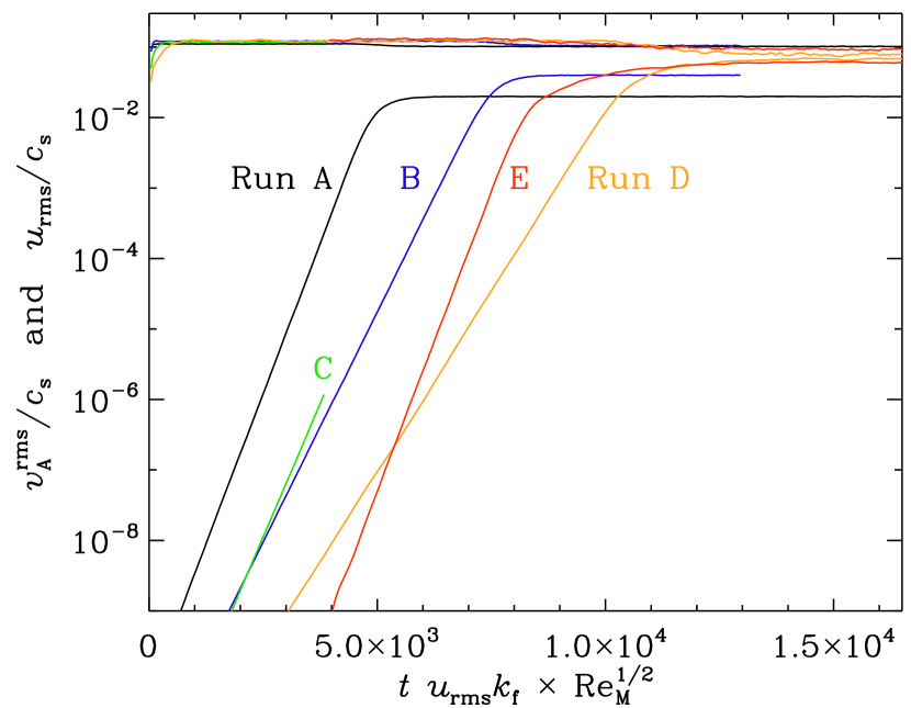
Figure 1: Time series of $u_{\rm rms}$ and $v_{\rm A}^{\rm rms}=B_{\rm rms}/\sqrt{\mu_{0}\rho_{0}}$, normalized by $c_{\rm s}$.

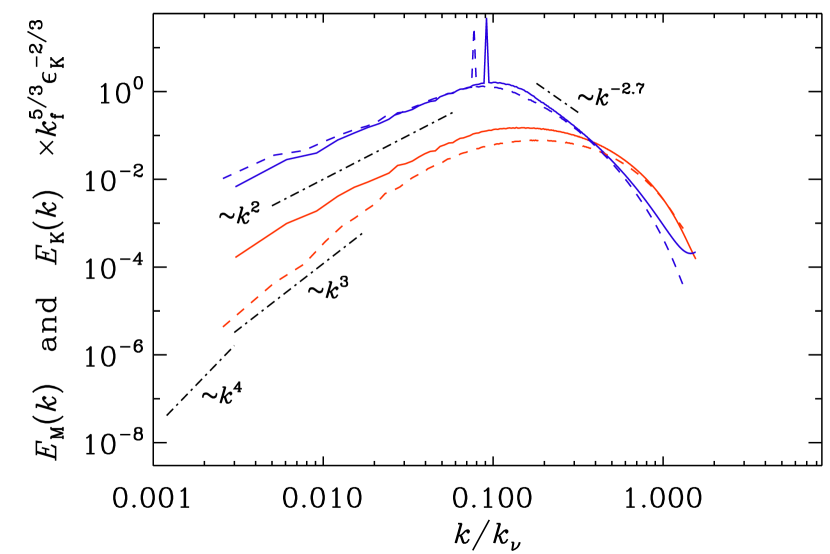
Figure 2: Kinetic (blue) and magnetic (red) energy spectra for Run B during the kinematic (dotted lines) and the saturated (solid lines) stages.

3.3 Emergence of the Kazantsev slope

We now consider Runs C and D with larger magnetic Prandtl numbers, $\mbox{\rm Pr}_{\rm M}=10$ and 30, respectively. Of these two runs, only Run D has been run into saturation, because we expect their nonlinear behaviors to be similar. In these runs, shown in Figs. 3 and 4, we also decrease the value of $k_{\rm f}$ to 10 and 4, respectively. In both cases, we clearly see the emergence of a Kazantsev $k^{3/2}$ subrange for $k>k_{\rm f}$. For Run D, we also see that the Kazantsev slope disappears in the saturated state. We show $k^{-5/3}$ slopes for comparison, but it is clear that there is insufficient dynamical range to identify a proper magnetic inertial range. We still see in the kinematic phase the $k^{3}$ subrange for $k<k_{\rm f}$. However, it is possible that the actual slope of the kinematic subrange spectrum is steeper, and that we just did not have enough scale separation between the lowest wavenumber $k_{1}$ and the forcing wavenumber $k_{\rm f}$. Therefore, we now consider a more extreme case with even more scale separation.

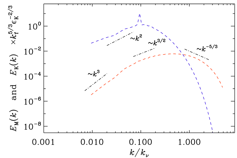
Figure 3: Similar to Fig. 2, but for Run C, except that the spectra are only shown for the kinematic phase.

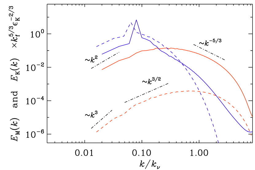
Figure 4: Similar to Fig. 2, but for Run D.

3.4 Batchelor spectrum in the kinematic stage

To see whether the $k^{3}$ subrange slope found in Sect. 3.2 was a consequence of still insufficient scale separation, we now consider a more extreme case with a four times larger value, namely $k_{\rm f}/k_{1}=120$; see Fig. 5. We now see that there is indeed a $k^{4}$ Batchelor subinertial range. Interestingly, we also see that near the very lowest wavenumbers in the domain, the spectrum does become slightly shallower. This suggests that the spectrum at those low wavenumbers, $1\leq k/k_{1}\leq 3$, is indeed contaminated by finite size effects of the computational domain.

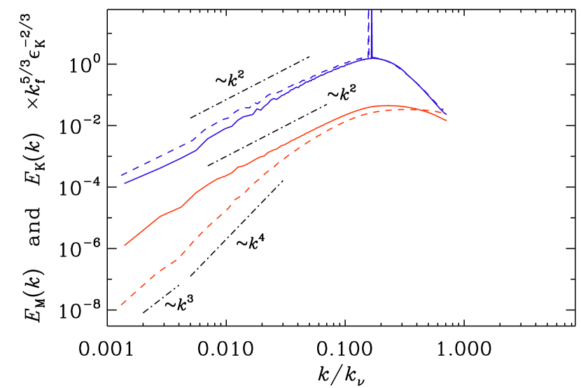
Figure 5: Similar to Fig. 2, but for Run A. Note the $k^{4}$ subrange of $E_{\rm M}(k)$ in the kinematic stage, but also evidence for slight contamination at very small $k$.

To demonstrate that the $k^{4}$ subrange existed throughout the entire kinematic phase, we show in Fig. 6 unnormalized spectra for Run A in regular time intervals during the kinematic stage and less frequently during the saturated stage, where the low wavenumber part is seen to grow slightly. The final slope during the saturated stages is $\propto k^{2}$, just like the kinetic energy spectrum; see Fig. 5.

Figure 6: Unnormalized spectra for Run A showing that the $k^{4}$ subrange existed throughout the entire kinematic phase.

The theoretical reason for the $k^{4}$ spectrum in the kinematic regime could lie in the statistical independence of different patches in space. This led Durrer & Caprini (2003) to suggest that primordial magnetic fields in the early Universe must always have a $k^{4}$ spectrum, as was already assumed in Christensson et al. (2001). The velocity field, by contrast, is driven by the magnetic field in a causal fashion, and it always shows a $k^{2}$ spectrum. When the magnetic field saturates, different patches are again no longer uncorrelated. This may explain the transition from a $k^{4}$ to a $k^{2}$ spectrum as a magnetic field saturates. To see the reason, note that for an isotropic turbulent magnetic field, its energy spectrum can be expanded at small $k$ as

$$E_{\text{M}}(k)=\frac{I_{B}k^{2}}{4\pi^{2}}+\frac{I_{L_{\text{M}}}k^{4}}{24\pi^{2}}+\mathcal{O}(k^{6}).$$ (9)

Here,

$$I_{B}=\int\left\langle\bm{B}(\bm{x})\cdot\bm{B}(\bm{x}+\bm{r})\right\rangle\ \text{d}^{3}r$$ (10)

and

$$I_{L_{\text{M}}}=-\int\left\langle\bm{B}(\bm{x})\cdot\bm{B}(\bm{x}+\bm{r})\right\rangle r^{2}\ \text{d}^{3}r$$ (11)

are the magnetic Saffman and magnetic Loitsyansky integrals, respectively (Hosking & Schekochihin, 2021). Thus a transition from $k^{4}$ to $k^{2}$ in the subinertial range for the magnetic energy spectrum suggests that $I_{B}$ has grown from zero to a finite value. This in turn implies that the magnetic field has built up some long-range correlations during nonlinear saturation, in the sense that $\left\langle\bm{B}(\bm{x})\cdot\bm{B}(\bm{x}+\bm{r})\right\rangle$ can decay as slowly as $r^{-3}$ as $r\to\infty$. Such long-range correlations might result from those of the velocity field, the latter being thoroughly discussed in Hosking & Schekochihin (2022).

3.5 Kazantsev spectrum at $\mbox{\rm Pr}_{\rm M}=1$

We recall that, in order to see the Kazantsev spectrum, we increased $\mbox{\rm Pr}_{\rm M}$ from one to 10 and 30, but we also decreased $k_{\rm f}/k_{1}$ from 30 to 10 and four. We now show that a larger value of $\mbox{\rm Pr}_{\rm M}$ was helpful in achieving dynamo action, but it was not essential for obtaining the Kazantsev spectrum. The important point is rather that the Kazantsev spectrum is really a small-scale phenomenon and is not present in the subinertial range. Therefore, all that is required is a long enough inertial range. To show this more clearly, we now present a case with $\mbox{\rm Pr}_{\rm M}=1$ and $k_{\rm f}/k_{1}=4$; see Fig. 7. We clearly see the Kazantsev spectrum during the kinematic stage of the dynamo.

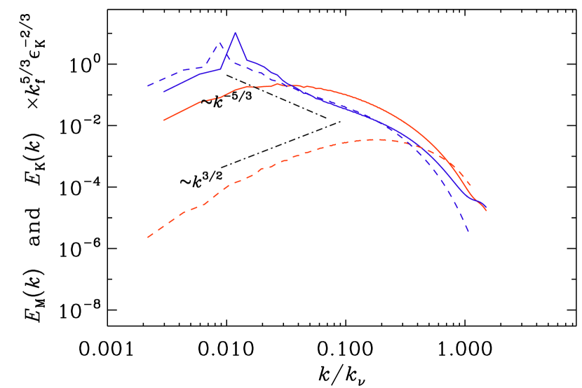
Figure 7: Similar to Fig. 2, but for Run E. Note the well developed $k^{3/2}$ Kazantsev slope for $E_{\rm M}(k)$ during the kinematic stage in the range where $E_{\rm K}(k)$ shows a $k^{-5/3}$ Kolmogorov subrange with bottleneck in the kinematic stage.

In Fig. 7, we also notice that, in the wavenumber interval with the Kazantsev slope in the magnetic energy spectrum, we also have a Kolmogorov inertial range in the kinetic energy spectrum together with a slight uprise near the dissipation wavenumber. This uprise is well known in turbulence theory and is referred to as the bottleneck effect (Falkovich, 1994). It is a phenomenon that is particularly clear in the three-dimensional spectra presented here, but it is less pronounced in the one-dimensional spectra considered in observations such as wind tunnel experiment, which has a simple mathematical reason (Dobler et al., 2003).

3.6 Inertial-range dynamo action

Run E has demonstrated that the Kazantsev spectrum extends well into the inertial range to length scales above the viscous scale. Is this truly caused by dynamo action in the inertial range or, perhaps, a nonlocal artifact caused by the strong spike in kinetic energy at the driving scale? As explained above, those peaks can be very large for large values of $k_{\rm f}/k_{1}$, although for Run E, this spike is no longer so pronounced. To analyze the spectral energy flux, we follow the procedure of Brandenburg et al. (2015) and compute the spectral transfers

$$T_{kpq}=\langle\bm{J}_{k}\cdot(\bm{u}_{p}\times\bm{B}_{q})\rangle\quad\mbox{and}\quad T_{kp}=\langle\bm{J}_{k}\cdot(\bm{u}_{p}\times\bm{B})\rangle.$$ (12)

Here, the subscripts on the vectors indicate linearly spaced wavenumbers of filtering over concentric shells in wavenumber space. In Fig. 8, we present the result for the kinematic stage. Figure 8(a) shows the energy spectra for velocity and magnetic fields, and the vertical lines mark the forcing scale at $k_{\rm f}/k_{1}=4$ (left), and the peak of the magnetic energy spectrum at $k_{\text{peak}}/k_{1}\simeq 81$ (right). In Fig. 8(b), we show the shell-to-shell transfer rates $T_{kp}$ at $k/k_{1}=43$, $110$, and $281$, which corresponds to $k/k_{\nu}=0.09$, $0.24$, and $0.61$. We see that there are strong peaks at the forcing scale, but also considerable contributions from smaller scales. Note that Fig. 8(b) is obtained by averaging $T_{kp}$ for $10$ snapshots, taken at intervals $\simeq 0.17/u_{\rm rms}k_{\rm f}$. For $k$ near or below $k_{\text{peak}}$, the contribution at $p=k_{\rm f}$ fluctuates, and sometimes becomes negative. This is because the velocity field at $k_{\rm f}$ is mostly driven by the random-in-time forcing, which rapidly changes its direction. At large $k$, near $k_{\nu}$, the velocity at that scale has become too small to drive dynamo action, and the energy transfer into the magnetic field mostly comes from the energy-dominant eddy at $k_{\rm f}$ tangling magnetic field lines. This explains the persistent and dominant peak for the blue curve in Fig. 8(b).

To identify where the dominant contribution comes from, we compute the accumulative transfer rate, $\int_{0}^{p}T_{kp^{\prime}}\text{d}p^{\prime}$; see Fig. 8(c). It is clear that the velocity modes in the inertial range contribute roughly equally to a given magnetic mode. Although the flow velocity has a strong peak near the forcing scale, it does not play a particularly significant role in the kinematic dynamo phase. In panel (d) we show the net transfer rate into shell $k$, $\int T_{kp}\text{d}p$, which scales as $k^{3/2}$ in the inertial range. Given that the magnetic energy spectrum is also $\propto k^{3/2}$ in the inertial range, this suggests that the dynamo growth rate $\text{d}\ln E_{\text{M}}/\text{d}t$ is independent of the wavenumber $k$, as would have been expected from the Kazantsev model, although, strictly speaking, the model is expected to be valid only for $\mbox{\rm Pr}_{\rm M}\gg 1$.

Figure 8: Results for run E. (a) The velocity and magnetic energy spectra at $t=300.4$. (b) The shell-to-shell energy transfer rate $T_{kp}$, for three selected values $k=43$, $110$, and $281$. (c) The accumulative transfer rate. (d) The net transfer rate. Data in panels (b), (c), and (d) is obtained by averaging over $10$ snapshots at $t=300.4,300.8,\cdots,304.0$.

4 Diagnostics of different subranges

4.1 Diagnostic images and spectra

In Fig. 9, we present for Run E synthetic radio images of $E(x,y)$, $B(x,y)$, and $\langle B_{z}\rangle_{z}(x,y)$, where the latter will simply be denoted by ${\rm RM}$. The structures are rather small, so we also show an enlarged presentation of $1/8^{2}$ of the image, as indicated by the white box on the corresponding full images.

Figure 9: Diagnostic slices of RM (top row), $E$ (middle row), and $B$ (bottom row), for Run E during the kinematic stage. The small white squares on the left column mark the part that is shown enlarged on the right column. All quantities are normalized by their rms value and the color bars for the enlarged frames are clipped at $\pm 2$ times the rms value, while those for the full frames are clipped at $\pm 4$ times the rms value.

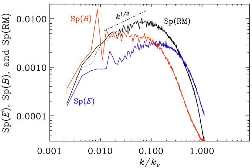
Figure 10: Diagnostic spectra $\mbox{\rm Sp}(E)$ (blue line), $\mbox{\rm Sp}(B)$ (red line), and $\mbox{\rm Sp}({\rm RM})$ (black line) for Run E during the kinematic stage. The dotted line gives $E_{\rm M}(k)/k$, normalized so that it nearly overlaps with $\mbox{\rm Sp}({\rm RM})$.

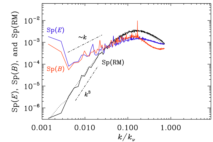
Figure 11: Same as Fig. 10, but for Run A during the kinematic stage.

Next, we present diagnostic spectra from our two-dimensional synchrotron images for Run E during the kinematic stage. They are denoted by $\mbox{\rm Sp}(E)$, $\mbox{\rm Sp}(B)$, and $\mbox{\rm Sp}({\rm RM})$ and are normalized such that $\int\mbox{\rm Sp}({\rm RM})\,{\rm d}{}k=1$ and $\int[\mbox{\rm Sp}(E)+\mbox{\rm Sp}(B)]\,{\rm d}{}k=1$; see Fig. 10. For comparison, we also overplot $E_{\rm M}(k)/k$, suitably normalized, which is seen to agree with $\mbox{\rm Sp}({\rm RM})$. It turns out that in $0.01\leq k/k_{\nu}\leq 0.1$, $\mbox{\rm Sp}({\rm RM})$ and $\mbox{\rm Sp}(E)$ are proportional to $k^{1/2}$. On the other hand, $\mbox{\rm Sp}(B)$ is flat; see Table 2 for the approximate wavenumber scalings of $E_{\rm M}(k)$, $\mbox{\rm Sp}({\rm RM})$, $\mbox{\rm Sp}(E)$, and $\mbox{\rm Sp}(B)$ for the inertial range of Run E.

For white noise in two dimensions, we would expect a linearly increasing spectrum. In the present case, this is indeed the case for the $E$ and $B$ polarizations in the subinertial range of Run A; see Table 3 and Fig. 11.

Table 2: Approximate wavenumber scalings of $E_{\rm M}(k)$, $\mbox{\rm Sp}({\rm RM})$, $\mbox{\rm Sp}(E)$, and $\mbox{\rm Sp}(B)$ for the subinertial range of Run A and the inertial range of Run E during the kinematic phase.

Run	range	$E_{\rm M}(k)$	$\mbox{\rm Sp}({\rm RM})$	$\mbox{\rm Sp}(E)$	$\mbox{\rm Sp}(B)$
A	subinertial	$k^{4}$	$k^{3}$	$k^{1}$	$k^{1}$
E	inertial	$k^{3/2}$	$k^{1/2}$	$k^{1/2}$	$k^{0}$

The correspondence between the exponent $\alpha$ in $E_{\rm M}(k)\propto k^{\alpha}$ and $\alpha_{{\rm RM}}$ in $\mbox{\rm Sp}({\rm RM})\propto k^{\alpha_{{\rm RM}}}$ with $\alpha_{{\rm RM}}=\alpha-1$ is explained by the line-of-sight integration, which removes the spatial dependence in one direction. For Run E, this is also seen for $\alpha_{E}$ in $\mbox{\rm Sp}(E)\propto k^{\alpha_{E}}$ with $\alpha_{E}=\alpha-1$. As already alluded to above, here, and also in the runs with a Kazantsev spectrum in the inertial range, $\mbox{\rm Sp}(B)$ shows a marked decline with $k$. It is surprising to have such a strong difference in the spectral properties between $E$ and $B$. This is probably explained by the mutual cancelation of opposite parities along the line of sight, which can only affect the parity-odd $B$ polarization, and would have been missed if one just looked at the Stokes $Q$ and $U$ polarizations.

Table 3: Diagnostic properties of Runs A–E. Except for run C, which has not saturated, the first and second lines for each run represent the kinematic and saturated phases, respectively. The characterization of elongated structures concerns the synchrotron $E$ polarization and is always absent for dust polarization. On the right, skewness and excess kurtosis are given for $E$ and $B$ during the kinematic and saturated stages.

							${\rm skew}(E)$		${\rm skew}(B)$		${\rm kurt}(E)$		${\rm kurt}(B)$
Run	$q_{\rm LS}^{\rm s}$	$q_{\rm SS}^{\rm s}$	$q_{\rm LS}^{\rm d}$	$q_{\rm SS}^{\rm d}$	elong. struct.	spectra	sync	dust	sync	dust	sync	dust	sync	dust
A	0.84	1.41	0.80	1.04	no; random	Batchelor	0.05	$-0.01$	0.00	$-0.00$	0.20	0.00	0.17	0.00
	0.87	1.18	0.80	0.76	no; random	Saffman	0.06	$-0.00$	$-0.00$	0.00	0.05	$-0.00$	$-0.07$	$-0.08$
B	0.66	3.3	0.48	1.13	marginal	$k^{3}$ and Saffman	0.36	$-0.03$	0.02	0.02	0.88	0.02	0.34	$-0.03$
	0.68	6.4	0.53	1.34	marginal	$k^{2}$	0.19	$-0.05$	$-0.00$	$-0.01$	0.20	0.01	0.03	$-0.00$
C	0.42	4.6	0.39	1.05	weakly	$k^{3}$ and short Kaz.	1.18	$-0.09$	0.03	$-0.03$	5.94	0.04	0.41	0.07
D	0.37	5.7	0.34	1.14	very clear	$k^{4}$ and Kazantsev	1.53	$-0.12$	$-0.20$	$-0.01$	7.66	0.01	0.39	0.12
	0.55	8.7	0.54	1.52	larger scale	$k^{2}$ and flat part	0.17	0.02	0.26	0.18	0.18	$-0.07$	0.62	0.10
E	0.63	3.0	0.34	1.18	somewhat	clear Kazantsev	0.51	$-0.03$	0.00	0.02	4.23	0.03	3.37	0.05
	0.82	70	0.57	1.61	larger scale	nearly flat	0.40	$-0.19$	0.17	0.09	0.38	$-0.04$	$-0.02$	$-0.19$

It is interesting to note that $\mbox{\rm Sp}(B)$ shows a strong decline near $k/k_{\nu}=0.1$, and it also shows a peak at $k_{\rm f}$. This suggests that the $B$ polarization reflects properties of the velocity field. The strong decline of $\mbox{\rm Sp}(B)$ toward large $k$ could therefore be a signature of the viscous cutoff.

One might have expected that the $E$ and $B$ spectra, which are quadratic in the magnetic field, have their peak at twice the wavenumber of the magnetic field spectra. This expectation was motivated by the fact that magnetic stress spectra occur at twice the peak wavenumber of the magnetic field itself (Brandenburg & Boldyrev, 2020). In particular, the peak of $\mbox{\rm Sp}(\bm{B}^{2})$ is twice that of $\mbox{\rm Sp}(\bm{B})$. This is not really seen in the present runs. Investigating the theoretical relations between the spectra of ${\cal B}$ and ${\cal B}^{2}$, for example, is clearly of interest, but beyond the scope of the present paper.

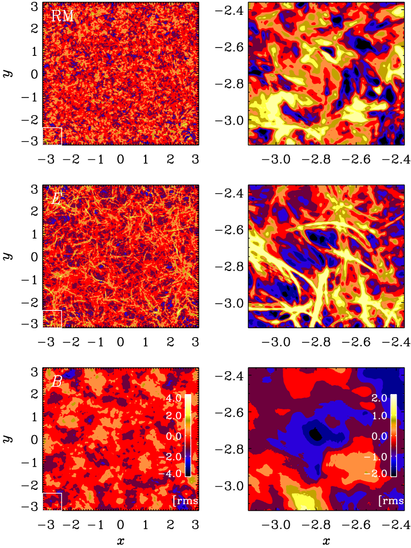
Figure 12: Same as Fig. 9, but for Run D during the kinematic stage.

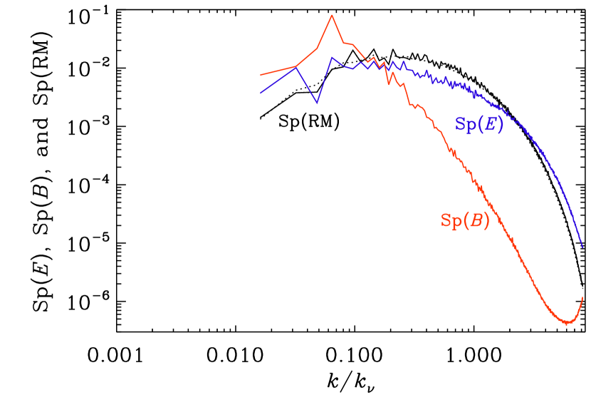
Figure 13: Same as Fig. 10, but for Run D during the kinematic stage.

For Run D, which has a large magnetic Prandtl number, we see very pronounced elongated structures in the $E$ polarization, which is not seen in the $B$ polarization, and only to some extent in RM; see Fig. 12. This corresponds with the spectra shown in Fig. 13, where $\mbox{\rm Sp}({\rm RM})$ and $\mbox{\rm Sp}(E)$ have a similar shape, but $\mbox{\rm Sp}(B)$ shows a sharp decline with increasing $k$.

4.2 Comparison with dust polarization

We recall that the main difference between synchrotron and dust emission lies in the fact that dust emission depends mostly on the dust temperature and not on the magnetic field strength (Planck Collaboration et al., 2015; Bracco et al., 2019). For dust emission, therefore, weak fields contribute just as much as strong fields. This is in sharp contrast to synchrotron emission, where the emissivity scales approximately quadratically with the magnetic field strength (Ginzburg & Syrovatskii, 1965). This causes systematic differences between the spectra from dust and synchrotron emission. Most remarkably, the elongated structures seen in the $E$ polarization of synchrotron emission are now absent; compare Fig. 12 with Fig. 14. Comparing the spectra in Figs. 13 and 15, we see that the excess power in $E$ is now absent. This is quantified in more detail in the next section.

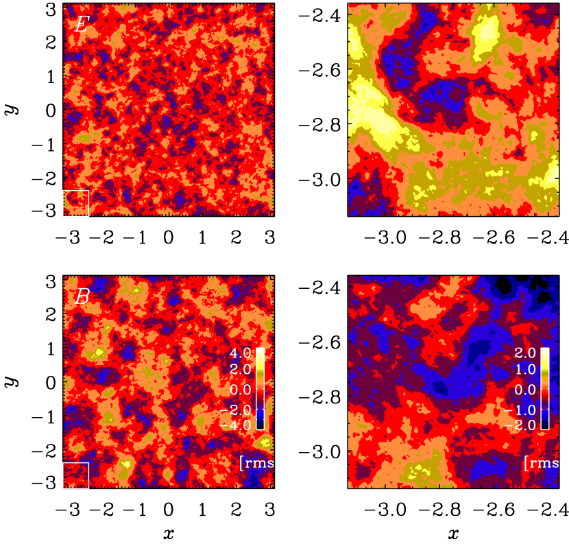
Figure 14: $E$ and $B$ for dust polarization from Run D.

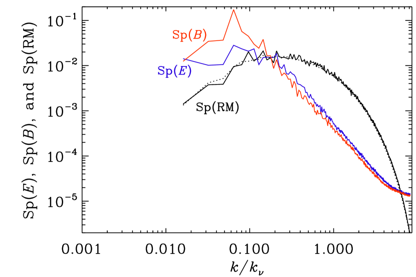
Figure 15: Same as Fig. 13, but for dust polarization.

4.3 Excess $E$ polarization in statistics

Of particular interest is the ratio $\langle E^{2}\rangle/\langle B^{2}\rangle$. As we saw from Fig. 10, the answer may depend on the wavenumber range for which the data is taken. For Runs D and E, the $E$ and $B$ spectra cross, and the crossing point $k_{\times}$ of the $E$ and $B$ spectra lies at $k_{\times}/k_{\nu}\approx 0.14$. It is therefore useful to compute the ratio separately for small and large $k$.

$$q_{\rm LS}\equiv\langle E^{2}\rangle_{\rm LS}/\langle B^{2}\rangle_{\rm LS}=\left.\int_{0}^{k_{\times}}\mbox{\rm Sp}(E)\,{\rm d}{}k\right/\int_{0}^{k_{\times}}\mbox{\rm Sp}(B)\,{\rm d}{}k,$$ (13)

$$q_{\rm SS}\equiv\langle E^{2}\rangle_{\rm SS}/\langle B^{2}\rangle_{\rm SS}=\left.\int_{k_{\times}}^{\infty}\mbox{\rm Sp}(E)\,{\rm d}{}k\right/\int_{k_{\times}}^{\infty}\mbox{\rm Sp}(B)\,{\rm d}{}k,$$ (14)

To distinguish the ratios for synchrotron and dust emission, we add superscripts s and d, respectively. The resulting ratios are listed in Table 3 both for synchrotron emission ($q_{\rm LS}^{\rm s}$ and $q_{\rm SS}^{\rm s}$) and for dust emission ($q_{\rm LS}^{\rm d}$ and $q_{\rm SS}^{\rm d}$), along with other observations about the runs. For synchrotron emission, the values of $q_{\rm SS}^{\rm s}$ can be rather large compared with the aforementioned factor of two. For dust polarization, the values are significantly smaller, although values of $q_{\rm SS}^{\rm d}$ of 1.5 and 1.6 can be seen for Runs D and E, respectively.

Earlier work on the $E$ and $B$ polarizations has shown a tendency for the probability functions (PDFs) of $E$ to be non-Gaussian and skewed, while the $B$ polarization was more nearly Gaussian (Brandenburg et al., 2019b; Brandenburg, 2019a), especially in decaying turbulence. In the present case, the result depends on the existence of an inertial range (Run E) and on whether the run is saturated or not. In Fig. 16 we show that for Run E, the PDFs correspond to stretched exponentials during the kinematic stage, with $E$ being also skewed, but both become nearly Gaussian during the saturated stage. For Run A, on the other hand, $E$ and $B$ are nearly Gaussian both during the kinematic and the saturated stages; see Fig. 17. Run D is closer to Run E than to Run A, but with the $E$ polarization being even more skewed during the kinematic stage; see Fig. 18. This could be a signature of the large magnetic Prandtl number in this case. In the second part of Table 3, we summarize the resulting values for skewness and (excess) kurtosis for all runs during the kinematic and saturated stages. For synchrotron emission, both the kurtosis and the skewness are particularly high for the runs with large magnetic Prandtl number (Runs C and D) during the kinematic phase. For Run E, the kurtosis of $E$ is also fairly large during the kinematic phase, but the skewness is now only 0.5. For this run, furthermore, even the kurtosis of $B$ is significant. For dust emission, on the other hand, both skewness and excess kurtosis are relatively small.

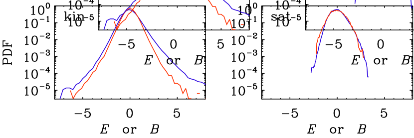
Figure 16: PDFs of $E$ (blue lines) and $B$ (red lines) during the kinematic (left) and saturated (right) stages for Run E.

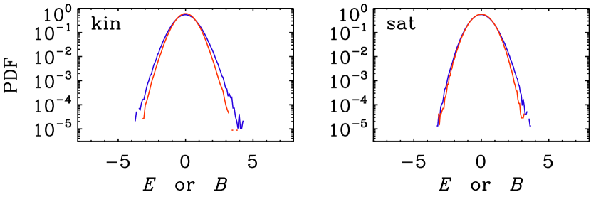
Figure 17: Same as Fig. 16, but for Run A.

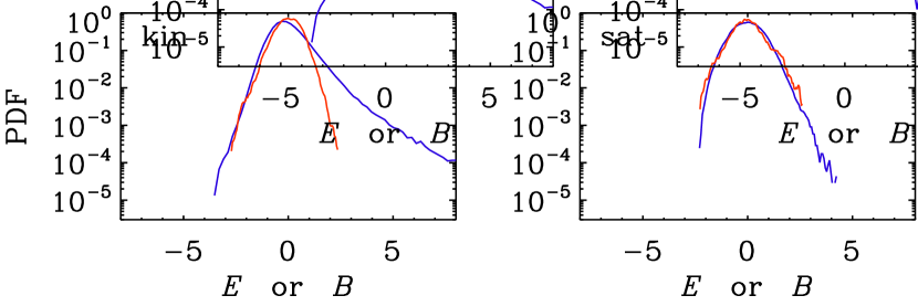
Figure 18: Same as Fig. 16, but for Run D.

For completeness, we present images and spectra of $E$, $B$, and RM for the other runs in Appendix B and in the supplemental material on Zenodo. The magnetic field tends to develop larger scale structures in the saturated state, which is also shown in this appendix.

5 Non-isothermal two-phase flows

To assess the robustness of our results to the assumption of an isothermal equation of state, we now consider a simulation with an ideal equation of state instead. This means that we must also include an evolution equation for the specific entropy, $s$, namely,

$$T{{\rm D}{}s\over{\rm D}{}t}=2\nu\mbox{\boldmath${\sf S}$}{}^{2}+{1\over\rho}{\bm{\nabla}}\cdot\left(c_{\rm p}\rho\chi{\bm{\nabla}}T\right)-{\cal L},$$ (15)

where $T$ is the temperature, $\chi$ is the thermal diffusivity, $c_{\rm p}$ is the specific heat at constant pressure, and ${\cal L}$ is the net cooling,

$${\cal L}=\rho\Lambda-\Gamma,$$ (16)

where $\Gamma=\mbox{const}$ is assumed for the heating function and $\Lambda(T)$ is the cooling function.

For the following model, we take the forced turbulence simulation setup of Brandenburg et al. (2007); see their Section 3.3. They adopted the piecewise power-law parameterization of Sánchez-Salcedo et al. (2002) for $\Lambda(T)$, but with slightly modified coefficients so as to avoid discontinuities; see Table 1 of Brandenburg et al. (2007). Also, the $c_{\rm s}^{2}{\bm{\nabla}}\ln\rho$ term in Eq. (2) now includes the specific entropy gradient, i.e., we replace

$$c_{\rm s}^{2}{\bm{\nabla}}\ln\rho\quad\longrightarrow\quad c_{\rm s}^{2}{\bm{\nabla}}(\ln\rho+s/c_{\rm p}),$$ (17)

where $c_{\rm s}^{2}=(\gamma-1)\,c_{\rm p}T$ is now no longer constant. Here, $\gamma=c_{\rm p}/c_{\rm v}=5/3$ is the ratio of specific heats, with $c_{\rm v}$ being the specific heat at constant volume. Note that $c_{\rm s}$ is related to $\ln\rho$ and $s$ via $c_{\rm s}^{2}=c_{\rm s0}^{2}[\gamma s/c_{\rm p}+(\gamma-1)\ln(\rho/\rho_{0})]$, where $c_{\rm s0}$ and $\rho_{0}$ are constants. Brandenburg et al. (2007) chose $c_{\rm s0}=1\,{\rm km\,s}^{-1}$ and $\rho_{0}=1\,m_{\rm H}\,{\rm cm}^{-3}$, where $m_{\rm H}$ is the mass of the hydrogen atom. They also chose $k_{1}=1\,{\rm kpc}^{-1}$, which fixes then the unit of time, although most of our results are presented in nondimensional form. The adopted cooling function allows for two stable fixed points of $c_{\rm s}\approx 1\,{\rm km\,s}^{-1}$ and $\approx 10\,{\rm km\,s}^{-1}$. When the initial density is in a suitable range (here $\rho=\rho_{0}$ initially) in the flow segregates into two phases, which is why we talk about a two-phase flow. Dynamos in such flows have recently been studied by Seta & Federrath (2022), who found a slight suppression of dynamo action due to the presence of two phases. We refer to our two-phase models as Run T0 and T1, where the numeral indicates the absence or presence of helicity in the forcing function, although there are several other difference between those two runs as well. Since we only consider the kinematic phase of the dynamo, the presence of helicity does not play an important role, because the large-scale dynamo would only emerge during saturation (Brandenburg, 2001).

The variability of the sound speed implies that in cool regions, the flow can become highly supersonic. On the average, however, the Mach number is around unity. The possibility of large Mach numbers requires the use of large viscosity and large thermal and magnetic diffusivities. Also, the simulations of Brandenburg et al. (2007) employed a helical forcing function, which helps lowering the threshold for dynamo action. We denote the fractional helicity of the forcing by $\sigma$, so $\sigma=1$ for Run T1, but we also present Run T0 with $\sigma=0$. Thus, our non-isothermal simulations are in many ways quite different from those presented in the rest of the paper and deserve proper analysis in a separate paper. Nevertheless, it is important to point out that the resulting images for RM, $E$ and $B$, shown in Fig. 19 for Run T0, are similar to those shown earlier in the paper. Also the spectra shown in Fig. 20 are similar, except that a sharp peak at the forcing scale is absent in $\mbox{\rm Sp}(B)$. The corresponding plots for Run T1 are shown in the supplemental material.

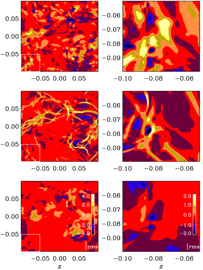
Figure 19: Same as Fig. 9, but for Run T0 during the kinematic stage.

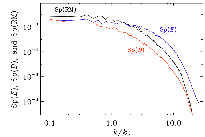
Figure 20: Same as Fig. 10, but for Run T0 during the kinematic stage.

Table 4: Summary of the parameters for Runs T0 and T1.

		Ma
Run	$\sigma$	rms, max	$\tilde{k}_{\rm f}$	$\tilde{k}_{\nu}$	$\tilde{\gamma}$	Re	$\mbox{\rm Re}_{\rm M}$	$\mbox{\rm Pr}_{\rm M}$
T1	1	8, 40	3	11	0.003	130	3800	30
T0	0	5, 20	4	10	0.001	150	4600	30

In this model, $\mbox{\rm Pr}_{\rm M}=10$; see Table 4 for a summary of parameters for this model. Consistent with the fact that the magnetic Prandtl number here is larger than unity, we find also here that the PDFs are skewed similarly as for Run D in Fig. 18. In addition to the different values of $\sigma$ for Runs T0 and T1, we used a five times smaller forcing amplitude for Run T0, but the Mach numbers are not so different. This is presumably caused by the two-phase nature of the flow. Indeed, it has been argued that two-phase flows can lead to sustained turbulence (Iwasaki & Inutsuka, 2014; Kobayashi et al., 2020), but clarifying this conclusively may require larger resolution and comparison with cases where the dynamical viscosity, $\rho\nu$, is held constant.

6 Conclusions

It is well known that in virtually all cases of astrophysical interest, Kolmogorov-type turbulence is always accompanied by dynamo action. This has consequences for the way turbulent energy is being dissipated into heat and radiation, which depends strongly on the value of the magnetic Prandtl number (Brandenburg, 2014; Brandenburg & Rempel, 2019). It is also well known that in the kinematic regime, the small-scale dynamo produces a characteristic spectrum known as the Kazantsev spectrum (Kazantsev, 1968), which was later discussed in more detail by Kulsrud & Anderson (1992). The Kazantsev spectrum is now also clearly seen in simulations (Schekochihin et al., 2004; Haugen et al., 2004). Our work has now shown that its spectrum extends over the full inertial range of the turbulence and that on larger, subinertial scales, one has a Batchelor spectrum, which turns into a Saffman spectrum as the dynamo saturates.

The fact that the Kazantsev spectrum extends over the full inertial range and not just over the subviscous range, $k_{\nu}\ll k\ll k_{\eta}$, is worth highlighting. Owing to limited numerical resolution, $k_{\nu}$ was in earlier numerical simulations often too close to the forcing wavenumber $k_{\rm f}$. This reinforced the theoretical expectation that small-scale dynamo action is confined to the wavenumber range where the flow is smooth (Schekochihin et al., 2004). On the other hand, in the inertial range, where the flow is “rough,” small-scale dynamos should still work, but they are much harder to excite (Rogachevskii & Kleeorin, 1997). This is the case at small $\mbox{\rm Pr}_{\rm M}$, when $k_{\eta}<k_{\nu}$ and the magnetic energy spectrum peaks in the inertial range. Since the work of Iskakov et al. (2007) we know that small-scale dynamos do indeed work for $\mbox{\rm Pr}_{\rm M}\ll 1$. A practical difficulty here lies in the fact that between the viscous and inertial subranges, there is the bottleneck range (Falkovich, 1994), where turbulence is even rougher than in the inertial range (Boldyrev & Cattaneo, 2004), making dynamo action even harder to demonstrate. This is not a problem in the magnetically saturated case, because then the bottleneck is suppressed (Brandenburg, 2011). In any case, for our Run E, we have $\mbox{\rm Re}_{\rm M}\approx 1600$, which should be large enough for the small-scale dynamo to be excited over the whole inertial range. Therefore, one should not be too surprised if the Kazantsev spectrum does indeed extend throughout the entire inertial range of the turbulence.

For synchrotron emission, our results suggest an excess $E$ polarization over the $B$ polarization at subresistive scales, and the opposite trend is found at larger scales. This is also found for the non-isothermal two-phase flows discussed in Sect. 5. For dust emission, on the other hand, the subviscous $E$ excess is much weaker, although values of 1.5 and 1.6 can be found for large magnetic Reynolds numbers.

An excess of the $E$ polarization is observed in the Galactic microwave foreground emission (Planck Collaboration et al., 2016; Caldwell et al., 2017). One might have expected the relevant scales to be much larger than the viscous scales. Observationally, however, one cannot exclude the possibility that the observed excess could result from subviscous scale. Furthermore, even in the saturated case, when the Kazantsev spectrum has disappeared, there is still an excess at subviscous scales. This numerical finding seems therefore remarkably robust.

Our study motivates new targets of investigation and new questions. How generic are the different realizations of turbulence found in the present study? Can we really expect the modeled types of velocity and magnetic fields to occur in galaxy clusters or in the ISM? One reason for concern is the fact that in all our flows, the driving is monochromatic with a typical wavenumber $k_{\rm f}$. Real turbulence may be more complicated. Nevertheless, the turbulence should always be characterized by a typical energy-carrying scale, $\xi_{\rm M}$, which defines an approximate position of the spectral peak at $k_{\rm f}\approx\xi_{\rm M}^{-1}$. It is therefore not obvious, that the monochromatic driving of our turbulence is actually very restrictive.

It is remarkable that the existence of the Kazantsev spectrum appears to be fairly insensitive to the value of the magnetic Prandtl number, but it never occurs at wavenumbers below the turbulent inertial range. Observing the transition to the steeper Batchelor spectrum requires very large domain sizes. This is why we allowed for a forcing scale that was up to 120 times shorter than the size of the domain (Run A). On the other hand, it is conceivable that in real cluster turbulence, the subinertial range is not entirely free of driving, as was assumed in the present work. However, clarifying this observationally could be difficult and may require full-sky observations to be able to identify the true peak of the spectrum.

Real galaxy cluster turbulence is believed to be driven by cluster mergers (e.g., Roettiger et al., 1999), and that the turbulence would be a state of decay in between such mergers events. An open question is therefore whether the Kazantsev spectrum can also be seen in decaying turbulence. There is no reason why not, but it is not easy to find and requires, as we have now seen, a sufficiently extended inertial range. On the other hand, a large magnetic Prandtl number is not required.

Our work has shown that differences between the parity-even $E$ and the parity-odd $B$ polarizations may serve to distinguish between Kazantsev and Batchelor spectra in synchrotron emission, provided the magnetic field is still (or again) in a kinematic growth phase. The best chance to find turbulence in a kinematic state may be in clusters in the beginning of a merger event, as alluded to above. However, our present work would need to be adapted to such situations to develop more realistic observational signatures specific to clusters turbulence.

All our runs with noticeable spectral differences between $E$ and $B$ had Kazantsev spectra in the inertial range. There were also cases where the PDFs were non-Gaussian with strong skewness in the $E$ polarization. Again, this does not occur for dust emission. Subviscous scales played a decisive role in producing excess $E$ polarization. It is unclear whether those are observationally accessible. Of course, if the observed excess $E$ polarization can only be explained as a subviscous phenomenon, it might just be this effect that would give us information about subviscous scales. Simulations by Kritsuk et al. (2018) for dust emission also produced excess $E$ polarization, but the reason behind this was not clear. Those simulations where ideal ones, so the viscous scale was an entirely numerical phenomenon in their simulations. Nevertheless, a more detailed spectral analysis might help shedding more light on the phenomenon of excess $E$ polarization. The strong skewness in the synchrotron $E$ polarization during the kinematic regime may have been caused by the elongated structures that are also clearly seen in images of $E$, provided $\mbox{\rm Pr}_{\rm M}$ is large. This is expected to be the case in the ISM and in galaxy clusters, which motivates further morphological and statistical studies of observed $E$ and $B$ polarizations. It is also striking that the $B$ polarization tends to reflect the velocity field and shows a peak at the driving scale. The $E$ polarization, by contrast, tends to peak at the wavenumber where the magnetic field is strong. This difference clearly sticks out in images showing larger scale structures of $B$ than those of $E$. This could be another characteristic signature detectable in the ISM.

Data Availability

The source code used for the simulations of this study, the Pencil Code (Pencil Code Collaboration et al., 2021), is freely available on https://github.com/pencil-code/. The DOI of the code is https://doi.org/10.5281/zenodo.2315093. The simulation setups and the corresponding secondary data, as well as supplemental material with additional plots for the PDFs of Run B and diagnostic images and spectra for Runs B and D in the saturated state are available on https://doi.org/10.5281/zenodo.6862459; see also https://www.nordita.org/~brandenb/projects/Kazantsev-Subinertial for easier access to the same material as on the Zenodo site.

Appendix A Changes during saturation

Table 5: Values of Ma, $\tilde{k}_{\nu}$, and $\tilde{\epsilon}_{\rm K}=\epsilon_{\rm K}/k_{1}c_{\rm s}^{3}$ during the kinematic and saturated stages.

Run	Ma	sat.	$\tilde{k}_{\nu}$	sat.	$\tilde{\epsilon}_{\rm K}$	saturated
A	0.111	0.102	764	718	$9.2\times 10^{-3}$	$7.2\times 10^{-3}$
B	0.121	0.105	389	328	$2.9\times 10^{-3}$	$1.5\times 10^{-3}$
C	0.118	…	106	…	$9.9\times 10^{-4}$	…
D	0.122	0.079	62	50	$4.1\times 10^{-4}$	$1.7\times 10^{-4}$
E	0.130	0.096	461	330	$3.6\times 10^{-4}$	$9.5\times 10^{-5}$

As the dynamo saturates, $u_{\rm rms}$, $k_{\nu}$, and $\epsilon_{\rm K}$ decrease by a certain amount that depends on the input parameters. This is demonstrated in Table 5, where we list the kinematic and saturated values for all five runs. We recall that Run C was not continued into saturation, which is here indicated by the ellipses.

Based on the values listed in Table 5, we can infer that the ratios of the saturated to the kinematic values depend either on $\mbox{\rm Re}_{\rm M}$ or on Re. Specifically, we see that $u_{\rm rms}({\rm sat})/u_{\rm rms}({\rm kin})$ decreases mainly with $\mbox{\rm Re}_{\rm M}$ like $\mbox{\rm Re}_{\rm M}^{-0.07}$, $k_{\nu}({\rm sat})/k_{\nu}({\rm kin})$ decreases like $\mbox{\rm Re}_{\rm M}^{-0.04}$, and $\epsilon_{\rm K}({\rm sat})/\epsilon_{\rm K}({\rm kin})$ decreases mainly with Re like $\mbox{\rm Re}^{-1/4}$.

Appendix B Diagnostics for other runs

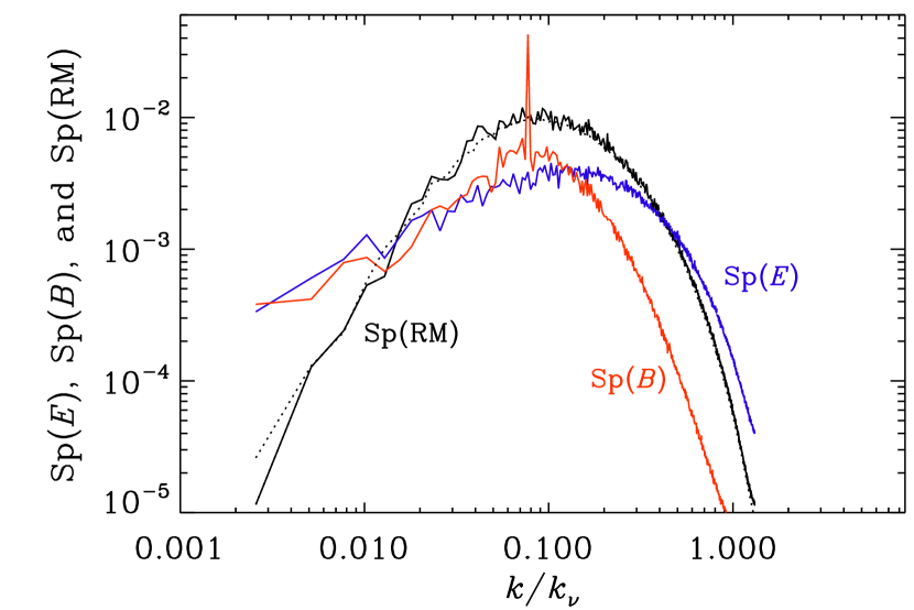
Figure 21: Same as Fig. 10, but for Run B during the kinematic stage.

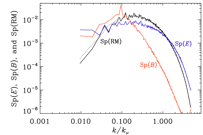
Figure 22: Same as Fig. 10, but for Run C during the kinematic stage.

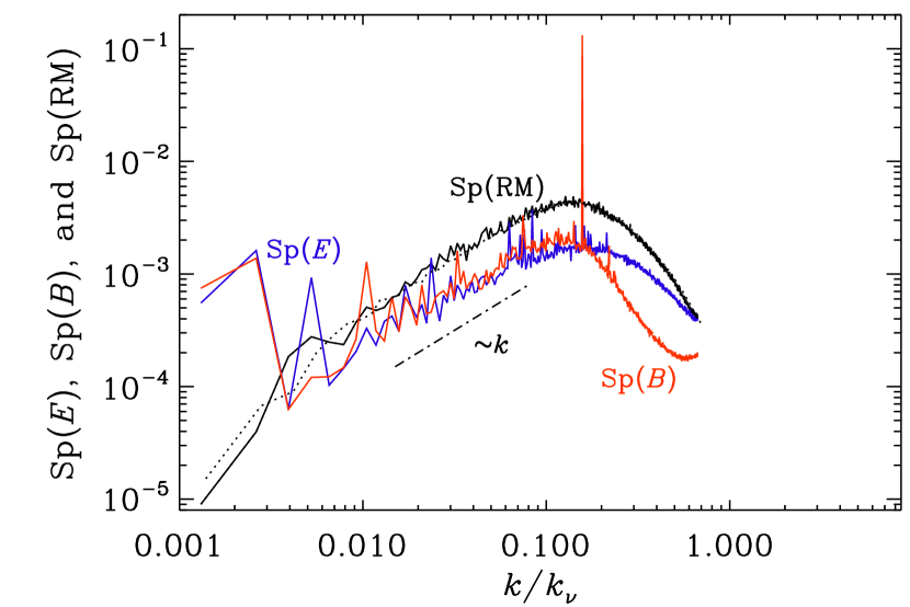
Figure 23: Same as Fig. 10, but for Run A during the saturated stage.

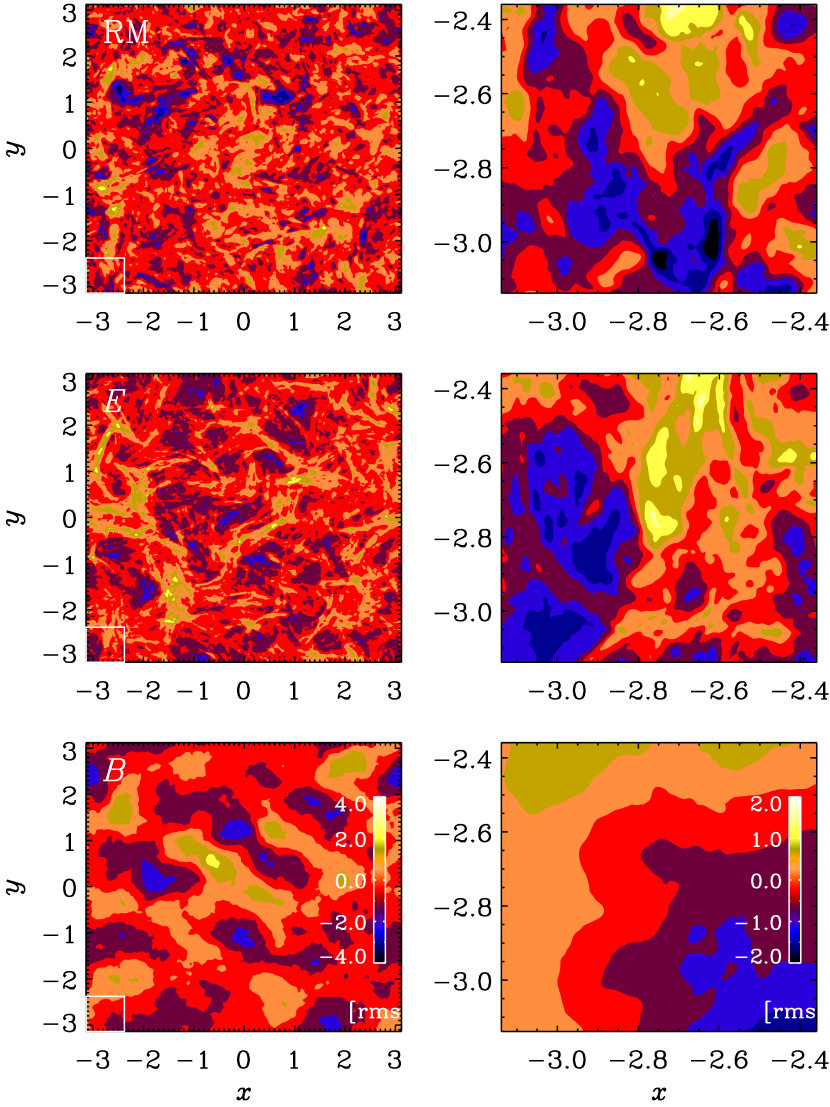
Figure 24: Same as Fig. 9, but for Run E during the saturated stage.

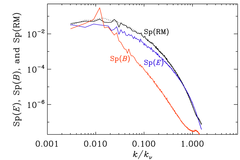
Figure 25: Same as Fig. 10, but for Run E during the saturated stage.

In Sect. 4.1, we presented diagnostic images and spectra for Runs E, A, and D. Here we also present spectra for Runs B and C; see Figs. 21 and 22. Between Runs B and C, we see a gradual increase in the elongated structures in $E$, which is typical for all runs with $\mbox{\rm Pr}_{\rm M}=1$. These are all for the kinematic stage, but in this appendix we also present results for the saturated stage of Runs A and E; see Figs. 23–25. During saturation, the most remarkable change is seen in the $B$ polarization of Run A, which consists of stripes that are inclined by $45\hbox{${}^{\circ}$}$. This is caused by a systematic dominance of vertical field components in the saturated state, which causes the formation of stacked clover leaf patches in the $B$ polarization, as was demonstrated previously in the appendix of Brandenburg & Furuya (2020).

References

- Banerjee & Jedamzik (2004) Banerjee R., Jedamzik K., 2004, PhRvD, 70, 123003
- Batchelor (1950) Batchelor G. K., 1950, Proc. Roy. Soc. Lond. Ser. A, 201, 405
- Bhat & Subramanian (2013) Bhat P., Subramanian K., 2013, MNRAS, 429, 2469
- Boldyrev (2005) Boldyrev S., 2005, ApJL, 626, L37
- Boldyrev (2006) Boldyrev S., 2006, PhRvL, 96, 115002
- Boldyrev & Cattaneo (2004) Boldyrev S., Cattaneo F., 2004, PhRvL, 92, 144501
- Bracco et al. (2019) Bracco A., Candelaresi S., Del Sordo F., Brandenburg A., 2019, A&A, 621, A97
- Brandenburg (2001) Brandenburg A., 2001, ApJ, 550, 824
- Brandenburg (2011) Brandenburg A., 2011, ApJ, 741, 92
- Brandenburg (2014) Brandenburg A., 2014, ApJ, 791, 12
- Brandenburg (2019a) Brandenburg A., 2019a, MNRAS, 487, 2673
- Brandenburg (2019b) Brandenburg A., 2019b, ApJ, 883, 119
- Brandenburg (2020) Brandenburg A., 2020, in Kosovichev A., Strassmeier S., Jardine M., eds, IAU Symp. Vol. 354, Solar and Stellar Magnetic Fields: Origins and Manifestations. pp 169–180 (arXiv:2004.00439), doi:10.1017/S1743921320001404
- Brandenburg & Boldyrev (2020) Brandenburg A., Boldyrev S., 2020, ApJ, 892, 80
- Brandenburg & Brüggen (2020) Brandenburg A., Brüggen M., 2020, ApJL, 896, L14
- Brandenburg & Furuya (2020) Brandenburg A., Furuya R. S., 2020, MNRAS, 496, 4749
- Brandenburg & Kahniashvili (2017) Brandenburg A., Kahniashvili T., 2017, PhRvL, 118, 055102
- Brandenburg & Rempel (2019) Brandenburg A., Rempel M., 2019, ApJ, 879, 57
- Brandenburg & Stepanov (2014) Brandenburg A., Stepanov R., 2014, ApJ, 786, 91
- Brandenburg et al. (1996) Brandenburg A., Enqvist K., Olesen P., 1996, PhRvD, 54, 1291
- Brandenburg et al. (2007) Brandenburg A., Korpi M. J., Mee A. J., 2007, ApJ, 654, 945
- Brandenburg et al. (2015) Brandenburg A., Kahniashvili T., Tevzadze A. G., 2015, PhRvL, 114, 075001
- Brandenburg et al. (2017) Brandenburg A., Kahniashvili T., Mandal S., Pol A. R., Tevzadze A. G., Vachaspati T., 2017, PhRvD, 96, 123528
- Brandenburg et al. (2018) Brandenburg A., Haugen N. E. L., Li X.-Y., Subramanian K., 2018, MNRAS, 479, 2827
- Brandenburg et al. (2019a) Brandenburg A., Kahniashvili T., Mandal S., Roper Pol A., Tevzadze A. G., Vachaspati T., 2019a, PhRvF, 4, 024608
- Brandenburg et al. (2019b) Brandenburg A., Bracco A., Kahniashvili T., Mandal S., Roper Pol A., Petrie G. J. D., Singh N. K., 2019b, ApJ, 870, 87
- Brandenburg et al. (2022) Brandenburg A., Rogachevskii I., Schober J., 2022, MNRAS, submitted, p. arXiv:2209.08717
- Caldwell et al. (2017) Caldwell R. R., Hirata C., Kamionkowski M., 2017, ApJ, 839, 91
- Cho & Ryu (2009) Cho J., Ryu D., 2009, ApJL, 705, L90
- Choi & Page (2015) Choi S. K., Page L. A., 2015, J. Cosmology Astropart. Phys., 2015, 020
- Christensson et al. (2001) Christensson M., Hindmarsh M., Brandenburg A., 2001, PhRvE, 64, 056405
- Dobler et al. (2003) Dobler W., Haugen N. E., Yousef T. A., Brandenburg A., 2003, PhRvE, 68, 026304
- Durrer & Caprini (2003) Durrer R., Caprini C., 2003, J. Cosmology Astropart. Phys., 2003, 010
- Falkovich (1994) Falkovich G., 1994, Phys. Fluids, 6, 1411
- Ginzburg & Syrovatskii (1965) Ginzburg V. L., Syrovatskii S. I., 1965, ARA&A, 3, 297
- Haugen et al. (2004) Haugen N. E., Brandenburg A., Dobler W., 2004, PhRvE, 70, 016308
- Hosking & Schekochihin (2021) Hosking D. N., Schekochihin A. A., 2021, PhRvX, 11, 041005
- Hosking & Schekochihin (2022) Hosking D. N., Schekochihin A. A., 2022, J. Fluid Mech., submitted, p. arXiv:2202.00462
- Iskakov et al. (2007) Iskakov A. B., Schekochihin A. A., Cowley S. C., McWilliams J. C., Proctor M. R. E., 2007, PhRvL, 98, 208501
- Iwasaki & Inutsuka (2014) Iwasaki K., Inutsuka S.-i., 2014, ApJ, 784, 115
- Kamionkowski et al. (1997) Kamionkowski M., Kosowsky A., Stebbins A., 1997, PhRvL, 78, 2058
- Kazantsev (1968) Kazantsev A. P., 1968, Sov. J. Exp. Theor. Phys., 26, 1031
- Kida et al. (1991) Kida S., Yanase S., Mizushima J., 1991, Phys. Fluids A, 3, 457
- Kobayashi et al. (2020) Kobayashi M. I. N., Inoue T., Inutsuka S.-i., Tomida K., Iwasaki K., Tanaka K. E. I., 2020, ApJ, 905, 95
- Krause & Rädler (1980) Krause F., Rädler K.-H., 1980, Mean-Field Magnetohydrodynamics and Dynamo Theory. Pergamon Press (also Akademie-Verlag: Berlin), Oxford
- Kritsuk et al. (2018) Kritsuk A. G., Flauger R., Ustyugov S. D., 2018, PhRvL, 121, 021104
- Kulsrud & Anderson (1992) Kulsrud R. M., Anderson S. W., 1992, ApJ, 396, 606
- Meneguzzi & Pouquet (1989) Meneguzzi M., Pouquet A., 1989, J. Fluid Mech., 205, 297
- Meneguzzi et al. (1981) Meneguzzi M., Frisch U., Pouquet A., 1981, PhRvL, 47, 1060
- Moffatt (1978) Moffatt H. K., 1978, Magnetic Field Generation in Electrically Conducting Fluids. Cambridge University Press, Cambridge
- Nordlund et al. (1992) Nordlund A., Brandenburg A., Jennings R. L., Rieutord M., Ruokolainen J., Stein R. F., Tuominen I., 1992, ApJ, 392, 647
- Olesen (1997) Olesen P., 1997, Phys. Lett. B, 398, 321
- Pacholczyk (1970) Pacholczyk A. G., 1970, Radio astrophysics. Nonthermal processes in galactic and extragalactic sources
- Pencil Code Collaboration et al. (2021) Pencil Code Collaboration et al., 2021, JOSS, 6, 2807
- Planck Collaboration et al. (2015) Planck Collaboration et al., 2015, A&A, 576, A105
- Planck Collaboration et al. (2016) Planck Collaboration et al., 2016, A&A, 586, A133
- Prabhu et al. (2020) Prabhu A., Brandenburg A., Käpylä M. J., Lagg A., 2020, A&A, 641, A46
- Prabhu et al. (2021) Prabhu A. P., Singh N. K., Käpylä M. J., Lagg A., 2021, A&A, 654, A3
- Reppin & Banerjee (2017) Reppin J., Banerjee R., 2017, PhRvE, 96, 053105
- Roettiger et al. (1999) Roettiger K., Stone J. M., Burns J. O., 1999, ApJ, 518, 594
- Rogachevskii & Kleeorin (1997) Rogachevskii I., Kleeorin N., 1997, PhRvE, 56, 417
- Saffman (1967) Saffman P. G., 1967, J. Fluid Mech., 27, 581
- Sánchez-Salcedo et al. (2002) Sánchez-Salcedo F. J., Vázquez-Semadeni E., Gazol A., 2002, ApJ, 577, 768
- Schekochihin (2022) Schekochihin A. A., 2022, J. Plasma Phys., 88, 155880501
- Schekochihin et al. (2004) Schekochihin A. A., Cowley S. C., Taylor S. F., Maron J. L., McWilliams J. C., 2004, ApJ, 612, 276
- Seljak & Zaldarriaga (1997) Seljak U., Zaldarriaga M., 1997, PhRvL, 78, 2054
- Seta & Federrath (2022) Seta A., Federrath C., 2022, MNRAS, 514, 957
- Seta et al. (2022) Seta A., Federrath C., Livingston J. D., McClure-Griffiths N. M., 2022, MNRAS,
- Steenbeck et al. (1966) Steenbeck M., Krause F., Rädler K. H., 1966, Zeitschr. Naturf. A, 21, 369
- Subramanian (2019) Subramanian K., 2019, Galaxies, 7, 47
- Subramanian & Brandenburg (2014) Subramanian K., Brandenburg A., 2014, MNRAS, 445, 2930
- Sur et al. (2018) Sur S., Bhat P., Subramanian K., 2018, MNRAS, 475, L72