SphereFed: Hyperspherical Federated Learning

Abstract

Federated Learning aims at training a global model from multiple decentralized devices (i.e. clients) without exchanging their private local data. A key challenge is the handling of non-i.i.d. (independent identically distributed) data across multiple clients that may induce disparities of their local features. We introduce the Hyperspherical Federated Learning (SphereFed) framework to address the non-i.i.d. issue by constraining learned representations of data points to be on a unit hypersphere shared by clients. Specifically, all clients learn their local representations by minimizing the loss with respect to a fixed classifier whose weights span the unit hypersphere. After federated training in improving the global model, this classifier is further calibrated with a closed-form solution by minimizing a mean squared loss. We show that the calibration solution can be computed efficiently and distributedly without direct access of local data. Extensive experiments indicate that our SphereFed approach is able to improve the accuracy of multiple existing federated learning algorithms by a considerable margin (up to 6% on challenging datasets) with enhanced computation and communication efficiency across datasets and model architectures.

1 Introduction

Federated learning (FL) is an emerging machine learning paradigm in which distributed clients learn on private data and communicate with a coordinating server to train a single global model that generalizes well across local data [51, 69]. One of its major challenges is the the handling of non-i.i.d. (independent identically distributed) local data across clients [32, 40, 42]. Non-i.i.d. local data leads to disparity of local models after learning on private data [94]. For instance, different feature extractors in local models may learn biased and discrepant input-to-feature mapping functions for the same class [18, 41, 89]. This obstructs the convergence of collaborative training.

Existing federated learning algorithms primarily tackle the non-i.i.d. problem in two phases: (i) In the local learning phase, regularization terms [2, 43, 80] and additive objectives [41, 84, 97] are used to control distances among local models via constraining the learning process. (ii) In the post-learning phase, the inevitable divergence of local models is corrected with additional information exchange [24, 32, 66, 79, 82] and advanced aggregation strategies such as normalized averaging [76], distillation [39], and so on [3, 5, 60, 87].

In this work, we argue that federated learning can also be improved in the pre-learning phase; this is a novel research direction complementary to existing approaches. A key insight is the use of a fixed classifier (e.g., the last fully-connected layer) that serves as a template of the feature extractor’s output for all clients. Note the loss function is often computed on the inner product between the feature vector (i.e., output of the feature extractor) and the classifier’s weight vectors. During local training, the feature extractor is optimized to project data from the $i$-th class to feature vectors that have the maximum inner product with the $i$-th of row of the classifier. We refer to the classifier as learning target of the feature extractor. However, higher data heterogeneity leads to a larger disparity of classifiers (in terms of both norms and directions) across clients. In this regard, if the local classifiers can be aligned, clients would have more consistent learning targets without modifying the learning procedure. Unfortunately, a real-time classifier synchronization carries prohibitively high communication overhead for federated learning. To avoid this communication cost, we use instead, for all clients, a fixed classifier constructed from orthonormal basis vectors.

Figure 1: Left: An overview of SphereFed (Hyperspherical Federated Learning). Before federated training starts, we construct a fixed shared classifier whose weight vectors span an unit hypersphere. After federated training ends, we calibrate the classifier in a distributed manner. Middle: All clients share the same hypersphere and learn to map local samples (markers represent clients) from the same class (colors represent classes) to the same area on the hypersphere whose centroid (the pentagram) corresponds to a weight vector. Right: Leveraging the linearity of the classifier, we derive its closed-form optimum which can be precisely computed by distributed clients. $Z^{\top}Z$ and $Z^{\top}Y$ are computed distributively because a matrix multiplication can be implemented as an accumulation of outer products and each outer product depends only on one client.

Motivated by this insight, we propose to construct a classifier whose weight vectors span an unit hypersphere before the federated training starts. Throughout federated training, this classifier is fixed and shared by all clients. Meanwhile, we also normalize the feature representation to the same hypersphere. During local learning, clients’ feature extractors learn to map data samples from the same class to the same area on the hypersphere whose centriod is the corresponding row vector of the classifier. As a result, the learned local features for data belonging to the same class are better aligned and the interference among local models are reduced, leading to an improved accuracy of the global model.

We name our approach Hyperspherical Federated Learning (SphereFed), which is a generic framework compatible with existing federated learning algorithms. An overview of the framework is illustrated in Fig. 1. SphereFed does not introduce extra hyper-parameters nor requiring additional computation. In fact, a pre-defined classifier eliminates the need of communication and brings improved efficiency to the system. Given that the classifiers are frozen during federated training, we propose to calibrate the classifier after federated training to achieve its optimum in a provable and lightweight manner. We first derive the closed-form optimum of the classifier leveraging its linearity and find that this closed-form solution can be precisely computed in a distributed manner without direct access to the private features (or data). We name this calibration method Fast Federated Calibration (FFC), which is provable and efficient compared with state-of-the-art methods (e.g., [48]) that depend on synthetically generated virtual features.

We conduct extensive experiments to demonstrate that the proposed SphereFed method is compatible with and complementary to several existing federated learning algorithms, capable of introducing up to 6% improvement on testing accuracy. Further experiments show that our proposed calibration achieves a performance gain comparable to the oracle fine-tuning with real features, verifying its theoretical optimality. A set of ablation studies are further presented to understand the efficacy of each design component in SphereFed.

2 Related Work

2.0.1 Standard Federated Learning.

Federated learning (FL) was originally proposed by [51, 69]. To address the non-i.i.d. problem, works have been pursued in two directions: imposing additional constraints in the local learning phase [43, 64, 66, 84] and conducting weight correction in the post learning phase [48, 60, 76, 87]. There have also been studies that tackle the non-i.i.d. issue by augmenting the on-client and on-server data with public [39] or synthetic [85, 97] samples.

Personalized Federated Learning. Personalized federated learning (pFL) differs from FL, by relaxing the setting of standard FL to allow each client to have its personalized local model via, e. g., additional local epochs after standard FL [11, 44]. In general, a personalized local model is more likely to obtain better accuracy on a local test set than the single global model, but the personalized local model could be more biased and less general to data from other sources [29, 77]. So, pFL and FL has different use focuses and application scenarios. Inspired from transfer learning [57, 86], a line of pFL methods learns local private parameters for the classifier but uses a shared feature extractor [7, 15, 70]. A concurrent and most related work is FedBABU which finds that fixing the classifier during collaborative learning is beneficial to the personalization process. Although this finding is consistent to our observations to some extent, our contribution is substantially different from FedBABU . First, we focus on FL while FedBABU focuses on pFL. Second, we ensure a stable performance gain resulting from an in-depth analysis on the benefit of fixing classifier. Third, we further propose a provable calibration method to improve the classifier after federated training.

Decoupling Layers for Federated Learning. Dealing layers at different depth with varying strategies has demonstrated effectiveness for many tasks in centralized training [23] like few-shot learning [65, 83], domain adaption [28, 75] and meta-learning [55, 59]. Such layer decoupling studies could also benefit federated learning applications. For instance, parameters from different layers can be updated and synchronized with different frequency to save communication cost [12, 13, 16]. FedRecon  [68] splits a model into global/local parts and reconstructs the local part on clients in each round to improve privacy and efficiency. FedUFO  [89] resorts an adversary module to reduce the divergence of feature extractors on clients. A most related work is CCVR  [48] which also focuses on the classifier. CCVR conducts on-server calibration for the classifier by fine-tuning it with virtual features sampled from Gaussian distributions. This work uses fundamentally different methodologies for the classifier and has higher performance gains and less communication/computation costs against CCVR .

Hyperspherical Representation. To the best of our knowledge, this is the first work introducing hyperspherical representation to address the non-i.i.d. challenge in FL. This combination is not trivial but motivated by analytical justifications and empirical supports as elaborated in the remaining sections. Hyperspherical representation has been widely adapted by studies on face recognition [45, 95], long-tail recognition [31], regression [52], metric learning [88, 96] and contrastive learning [33] to enhance the discriminative power of features. In this work, under the context of FL, we use hyperspherical features with fixed targets to align the learning objectives and minimize cross-party interference.

3 Federated Learning with Non-i.i.d. Clients

3.1 Terminologies

We consider $K$ clients and a central server in a federated learning system. Each client $k\in[K]$ has a local and private dataset $\mathcal{D}^{k}$. We focus on the non-i.i.d. data setting where local datasets could have heterogeneous distributions [40]. The goal is to train a single global classification model collaboratively which performs well on the global test set. The loss function is represented using $\mathcal{L}(\cdot,\cdot)$.

For a single training example $\left({\mathbf{x}},y\right)$, let ${\mathbf{z}}=f_{\theta}({\mathbf{x}})\in\mathbb{R}^{l}$ denote the $l$-dimension feature vector given a feature extractor $f_{\theta}(\cdot)$ parameterized by $\theta$. The classifier $h_{\mathbf{W}}(\cdot)$ takes ${\mathbf{z}}$ as input and makes the final prediction after a linear transformation ${\textnormal{o}}=h_{\mathbf{W}}({\mathbf{z}})={\mathbf{W}}{\mathbf{z}}+{\mathbf{b}}$ with a weight matrix ${\mathbf{W}}\in\mathbb{R}^{C\times l}$, where $C$ is the number of classes. For simplicity, we omit the bias term ${\mathbf{b}}$ in future equations.

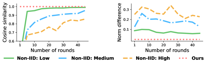
Figure 2: Direction and norm alignment of classifiers’ weights across clients. For the sake of simplicity, we train ResNet18 on CIFAR-100 with 10 clients for 50 rounds, using FedAvg in this empirical study. The non-i.i.d. level is controlled by the concentration parameter of a Dirichlet distribution [32, 40, 42]. There is a clear negative correlation between non-i.i.d. level and consistency of classifiers’ weights across clients, which incurs inconsistent local learning targets.

3.2 Non-i.i.d. Data Leads to Inconsistent Local Learning Targets

In each round of standard federated learning, each client optimizes the feature extractor and the classifier $(\theta,{\mathbf{W}})$ jointly. Then each client sends its updated feature extractor and classifier $(\theta^{k},{\mathbf{W}}^{k})$ to the central server which aggregates (e.g., averages [51]) all received local models into a single global one used for the next round. Prior studies [40] focus on either the local training loss function or an advanced aggregation strategy.

In this work, we pay special attention to the classifier. A classifier is the closet layer to the loss function and the $i$-th row of its weights ${\mathbf{w}}_{i}^{k}$ acts as a feature template and the learning target of the $i$-th class for the feature extractor. As a result, the disparity of classifiers across clients induces inconsistent local learning targets and further engenders local feature extractors’ disparity. A performance degradation may occur after aggregation in the central server.

The above hypothesis is verified by empirical observations. To show that, we rewrite the output of the classifier as,

$$\scalebox{0.9}{${\mathbf{W}}^{k}{\mathbf{z}}=\left[{\mathbf{w}}^{k}_{1}{\mathbf{z}},\dots,{\mathbf{w}}^{k}_{i}{\mathbf{z}},\dots,{\mathbf{w}}^{k}_{C}{\mathbf{z}}\right],\text{ where }{\mathbf{w}}^{k}_{i}{\mathbf{z}}=\|{\mathbf{w}}_{i}^{k}\|\|{\mathbf{z}}\|\cdot\cos{\left(\angle\left({\mathbf{w}}_{i}^{k},{\mathbf{z}}\right)\right)}$ }.$$ (1)

$\angle(\cdot,\cdot)$ denotes the angle between two vectors and $\|\cdot\|$ is the euclidean norm of a vector. A local feature extractor $f_{\theta}^{k}$ learns to maximize the output of the ground-truth class, ${\mathbf{w}}_{i}^{k}{\mathbf{z}},\ \forall i=y$, and minimize outputs of other classes ${\mathbf{w}}_{j}^{k}{\mathbf{z}},\ \forall j\neq y$. In summary, Eq. 1 highlights that both norms and directions of classifier’s weight vectors impact the optimization of feature extractor and thus (at least partially) effect the distribution of features generated by the feature extractor.

We empirically find that there is a clear negative correlation between non-i.i.d. degree and the consistency of classifiers’ weights (in terms of both norm and direction) across clients. We compute the cosine similarity (Eq. 2 and Fig. 2, Left) and norm difference (Eq. 3 and Fig. 2, Right) of classifier weight vectors for the same class but from arbitrary two different clients ($k_{1}\neq k_{2}$ and $1\leq k_{1},k_{2}\leq K$) using FedAvg [51].

$\mathbb{E}_{c\sim[C],k_{1}\neq k_{2}}\left[\frac{{\mathbf{w}}_{c}^{k_{1}}\cdot{\mathbf{w}}_{c}^{k_{2}}}{\|{\mathbf{w}}_{c}^{k_{1}}\|\|{\mathbf{w}}_{c}^{k_{2}}\|}\right]$ (2)

$\mathbb{E}_{c\sim[C],k_{1}\neq k_{2}}\left[\left|\|{\mathbf{w}}_{c}^{k_{1}}\|-\|{\mathbf{w}}_{c}^{k_{2}}\|\right|\right]$ (3)

According to Fig. 2, data with a higher degree of non-i.i.d. is associated with less direction alignment and larger magnitude difference of classifier weight vectors among clients, which lead to weaker consistency of the local learning targets. This will further engender non-overlapped feature distributions for the same class on different clients as illustrated in Fig. 3 (Left).

4 Hyperspherical Federated Learning

4.1 Hyperspherical Representation

A simple yet effective tweak to bypass the aforementioned issue is to align features from clients on a hypersphere, aided by a fixed classifier. In Eq. 1, we show that both the norm and the direction of $k$-th weight vector ${\mathbf{w}}_{i}^{k}$ play crucial roles in the learning of $f_{\theta^{k}}$ but a non-i.i.d. data distribution causes a disorder of norms and directions. To tackle this problem, we consider to construct ${\mathbf{W}}^{k}=\{{\mathbf{w}}_{i}^{k}\}^{C}_{i=1}$ manually, which has a unit norm and orthogonal components,

Note that $\smash{\{{\mathbf{w}}_{i}^{k}\}^{C}_{i=1}}$ span an $l$-dimension unit hypersphere. The orthogonality among $\smash{\{{\mathbf{w}}_{i}^{k}\}^{C}_{i=1}}$ ensures the maximum separation between arbitrary pair of classes. In addition, the uniformly unit norm guarantees balance in classes. Feature normalization is further adapted to project feature vectors on the same unit hypersphere, $\tilde{{\mathbf{z}}}={{\mathbf{z}}}/{\|{\mathbf{z}}\|}$. Normalizing features enables $f_{\theta}^{k}$ to focus on learning feature vectors’ directions and makes federated training process more robust to feature magnitude. Given a data point $\left({\mathbf{x}},y\right)$, a feature extractor $f_{\theta^{k}}$ maps the input ${\mathbf{x}}$ to a feature vector $f_{\theta^{k}}({\mathbf{x}})/\|f_{\theta^{k}}({\mathbf{x}})\|$ on the unit hypersphere, using the corresponding weights ${\mathbf{w}}^{k}_{y}$ as the target of mapping.

To ensure that all clients have the same learning targets (i.e., the same classifier $h_{{\mathbf{W}}^{k}}$), we share the constructed ${\mathbf{W}}^{k}$ with all clients and keep the shared ${\mathbf{W}}^{k}$ fixed throughout the federated training process. By doing this, local classifiers become consistent automatically without costly frequent inter-client synchronization. Since all clients now share the same learning targets, different local feature extractors on clients learn to map local data samples from the $i$-th class to the same area on the hypersphere with ${\mathbf{w}}_{i}^{k}$ as the centroid of that area. As a result, the norms and directions of local features are aligned with reduced interference across clients. In addition, the features from different classes have minimized overlaps and balanced magnitudes. An illustration of hyperspherical features can be found in Fig. 1 (Middle).

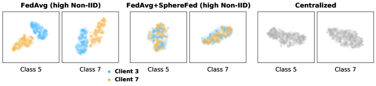
Figure 3: A qualitative study of Hyperspherical Federated Learning (SphereFed). In the left and middle sub-figures, dots in different colors represent features of the same class but generated by local models $f_{\theta^{k}}$ of different clients. SphereFed encourages consistency among clients’ features by aligning local learning targets.

The benefits of adapting the proposed hyperspherical features (and each design component described above) are revealed in a qualitative evaluation (Fig. 3). For more detailed ablation study including quantitative results, please refer to Sec. 5.3. In Fig. 3, we plot a certain class’s features from different clients to visualize local features alignment across clients. Three kinds of methods are compared including FedAvg [51] (with conventional classifier), standard centralized training, and SphereFed. We use MobileNetV2 for all three methods. For FedAvg and SphereFed, we partition the CIFAR-100 dataset to 10 clients according to the Dirichlet distribution with the concentration parameter $\alpha$ set as $0.1$ to simulate the high non-i.i.d. scenario. For the sake of visualization, we randomly select two clients (e.g., the 3-rd and 7-th clients in Fig. 3) and use their local models (at the $90$-th round) to generate features of two random classes (e.g., the class 5 and 7 in Fig. 3) . For centralized training, we train MobileNetV2 for 120 epochs to convergence and use the learnt model to generate features. The dimension of raw features is 1280 and we use t-SNE [49] to reduce the dimension to 2 for visualization. According to Fig. 3, in FedAvg, local models learn divergent mapping functions and thus features from the same class but different clients are biased to different distributions (i.e., non-overlapped clusters in Fig. 3). While, our hyperspherical features aligns well across clients as the centralized training (i.e., fused clusters in Fig. 3).

4.2 Using Mean Squared Error Loss on Hyperspherical Features

A widely accepted training method for classification tasks is to apply the softmax function [6] to the classifier output ${\mathbf{W}}^{k}{\mathbf{z}}$ before calculating the cross entropy (CE) loss. Combination of CE and softmax function is known to be sensitive to the scale of its input [23, 74]. However, in SphereFed, the classifier’s output, has less-than-one scale because of unit weights and hyperspherical features. To mitigate such a scaling issue, prior work for centralized training adopts either a pre-defined [14, 74] or a learnable [23, 31] scaling parameter $\tau$ in $\tau\cdot{\mathbf{W}}^{k}{\mathbf{z}}$ (i.e., temperature) to stabilize optimization. Unfortunately, performing a grid search on the scaling hyper-parameter would add significant communication and computation overheads in the setting of federated learning. A freely learnable scaling parameter could also aggravate local models’ disparity when the clients have different scaling parameters.

Interestingly, historical [19, 63] and recent [4, 27, 34] studies show competitive results of mean square error (MSE) [10] compared with CE for classification tasks on modern deep architectures. We refer readers to [53] and the related literature [8, 50, 72] for a more in-depth theoretical discussion. In this work, we use MSE to learn hyperspherical features to bypass the scaling issue of CE, i.e.,

where $\bm{1}\small(i=y)$ is equal to 1 if and only if $i=y$, $C$ is the number of classes, and $\texttt{one\_hot}(\cdot)$ is the one-hot vector representation of a label.

4.3 Fast Federated Calibration (FFC)

Throughout federated training of the hyperspherical representation, the weight of classifier ${\mathbf{W}}^{k}$ is fixed to help align learning targets of local features. So naturally, after federated training, a calibration on the classifier could be useful in improving the accuracy of the resulting global model. We, in turn, fix the learnt global feature extractor and calibrate the global classifier to boost the performance of the global model.

An interesting effect of using MSE loss in conjunction with a linear classifier is that we are able to calculate the unique closed-form optimum of classifier’s weight matrix given the input of the linear classifier. Formally, the objective of calibrating the classifier ${\mathbf{W}}$ is,

$$\scalebox{0.85}{$\operatorname*{arg\,min}_{\mathbf{W}}\ \mathbb{E}_{({\mathbf{x}},y)\sim\mathcal{D}}\left[\mathcal{L}_{\textrm{{\tiny MSE}}}\left({\mathbf{W}}{\mathbf{z}},\ y\right)\right],\quad\textrm{where}\ {\mathbf{z}}={f_{\theta}({\mathbf{x}})}/{\|f_{\theta}({\mathbf{x}})\|}\ \,\textrm{and}\ \,\mathcal{D}=\bigcup_{k\in[K]}\mathcal{D}^{k}$ }~{}.$$ (6)

We temporarily remove the superscripts of $(\theta,{\mathbf{W}})$ to emphasize that we consider the global feature extractor and global classifier. We refer to $\mathcal{D}$ as the whole dataset which consists of all local training data. Eq. 6 is essentially a least square problem, which has a closed-form solution, i.e.,

$$\scalebox{0.8}{${\mathbf{W}}^{*}=\left({\mathbf{Z}}^{\top}{\mathbf{Z}}\right)^{-1}{\mathbf{Z}}^{\top}{\mathbf{Y}}$ }.$$ (7)

The $i$-th row of ${\mathbf{Z}}$ is the normalized feature vector ${{\mathbf{z}}}_{i}$ corresponding to the $i$-th sample ${\mathbf{x}}_{i}$ in $\mathcal{D}$. Similarly, the $i$-th row of ${\mathbf{Y}}$ is the one-hot target vector $\texttt{one\_hot}(y_{i})$ corresponding to ${\mathbf{x}}_{i}$.

Obtaining ${\mathbf{Z}}$ (and ${\mathbf{Y}}$) requires all clients to upload their features (and corresponding labels). However, in the context of federated learning, sharing features and labels will cause prohibitively expensive communication overheads and potential model inversion attack [17, 93]. To achieve efficient and privacy-enhanced calibration, we propose to compute ${\mathbf{W}}^{*}$ in a distributed manner. It is inspired by that matrix multiplication can be implemented by a sum of outer products [92, 46]. Take ${\mathbf{Z}}^{\top}{\mathbf{Z}}$ as an example. We can rewrite the ${\mathbf{Z}}^{\top}{\mathbf{Z}}$ as a sum of outer products between columns of ${\mathbf{Z}}^{\top}$ and lrows of ${\mathbf{Z}}$ such that

$${\mathbf{Z}}^{\top}{\mathbf{Z}}=\underbrace{\mathchoice{\leavevmode\hbox to7.24pt{\vbox to8.05pt{\text{[drawing]}}}}{\leavevmode\hbox to7.24pt{\vbox to8.05pt{\text{[drawing]}}}}{\leavevmode\hbox to5.07pt{\vbox to5.64pt{\text{[drawing]}}}}{\leavevmode\hbox to3.62pt{\vbox to4.03pt{\text{[drawing]}}}}\otimes\mathchoice{\leavevmode\hbox to17.82pt{\vbox to8.05pt{\text{[drawing]}}}}{\leavevmode\hbox to17.82pt{\vbox to8.05pt{\text{[drawing]}}}}{\leavevmode\hbox to12.48pt{\vbox to5.64pt{\text{[drawing]}}}}{\leavevmode\hbox to8.91pt{\vbox to4.03pt{\text{[drawing]}}}}+\ \dotsi}_{\textbf{Client 1}}\ \dotsi\ \underbrace{\vphantom{a_{a_{a_{a_{a}}}}^{b}}\dotsi\ +\ \dotsi}_{\textbf{Client k}}\ \dotsi\ {\underbrace{\vphantom{a^{b}}\dotsi+\mathchoice{\leavevmode\hbox to20.15pt{\vbox to8.68pt{\text{[drawing]}}}}{\leavevmode\hbox to20.15pt{\vbox to8.68pt{\text{[drawing]}}}}{\leavevmode\hbox to14.11pt{\vbox to6.08pt{\text{[drawing]}}}}{\leavevmode\hbox to10.08pt{\vbox to4.34pt{\text{[drawing]}}}}\otimes\mathchoice{\leavevmode\hbox to20.15pt{\vbox to8.68pt{\text{[drawing]}}}}{\leavevmode\hbox to20.15pt{\vbox to8.68pt{\text{[drawing]}}}}{\leavevmode\hbox to14.11pt{\vbox to6.08pt{\text{[drawing]}}}}{\leavevmode\hbox to10.08pt{\vbox to4.34pt{\text{[drawing]}}}}}_{\textbf{Client K}}}~{}. {{\mathbf{z}}}_{1}^{\top} {{\mathbf{z}}}_{1}^{\top} {{\mathbf{z}}}_{1} {{\mathbf{z}}}_{1}^{\top} \smash{{{\mathbf{z}}}_{{{|\mathcal{D}|}}}^{\top}} {{\mathbf{z}}}_{1}^{\top} \smash{{{\mathbf{z}}}_{{{|\mathcal{D}|}}}} {{\mathbf{z}}}_{1}^{\top} {{\mathbf{z}}}_{1}^{\top} {{\mathbf{z}}}_{1} {{\mathbf{z}}}_{1}^{\top} \smash{{{\mathbf{z}}}_{{{|\mathcal{D}|}}}^{\top}} {{\mathbf{z}}}_{1}^{\top} \smash{{{\mathbf{z}}}_{{{|\mathcal{D}|}}}}$$ (8)

As a result, to calculate ${\mathbf{Z}}^{\top}{\mathbf{Z}}$, each client can complete a fraction of sum over their local features (as shown in Eq. 8) and upload the intermediate results to the sever to finish the computation, rather than upload private local features ${{\mathbf{z}}}_{i}$. In addition, the computation of ${\mathbf{Z}}^{\top}{\mathbf{Y}}$ in Eq. 7 can be calculated in the same way. See Fig. 1 (Right) for a vivid illustration.

Algorithm. We elaborate the FFC algorithm below:

1. On clients: Each client receives the latest global feature extractor $f_{\theta}$ from the server and computes the ${\mathbf{V}}^{k}\in\mathbb{R}^{l\times l},\ {\mathbf{U}}^{k}\in\mathbb{R}^{l\times C}$ on its local data $\mathcal{D}^{k}$,

   $$\scalebox{0.9}{${\mathbf{V}}^{k}=\sum_{i=1}^{|\mathcal{D}^{k}|}\,{{\mathbf{z}}}_{i}^{\top}{{\mathbf{z}}}_{i},\quad{\mathbf{U}}^{k}=\sum_{i=1}^{|\mathcal{D}^{k}|}{{\mathbf{z}}}_{i}^{\top}\texttt{one\_hot}(y_{i})$ },$$ (9)

   where ${{\mathbf{z}}}_{i}=f_{\theta}({\mathbf{x}}_{i})/\|f_{\theta}({\mathbf{x}}_{i})\|$ and $({\mathbf{x}}_{i},y_{i})\sim\mathcal{D}^{k}$.

2. On server: The server receives all $\{({\mathbf{V}}^{k},{\mathbf{U}}^{k})\ |\ k\in[K]\}$ from clients and computes the closed-form weights optimum,

   $$\scalebox{0.85}{${\mathbf{W}}^{*}=\left(\sum_{k=1}^{K}{\mathbf{V}}^{k}\right)^{-1}\left(\sum_{k=1}^{K}{\mathbf{U}}^{k}\right)$ }.$$ (10)

Table 1: Comparison of communication and computation costs for the classifier over 10 clients for 100 rounds. We assume that communicated weights are in 32-bit. The number of FLOPs is computed by considering both clients (“(C)”) and the server (“(S)”). Since all approaches require forward of the classifier, we exclude it from calculation. “Every” (and “Once”) means communicating at every round (and only once).

Method	Communication			Computation		Accuracy
	Objects	Frequency	Size (MB)	Operation	FLOPs (G)
FedAvg	${\mathbf{W}}\in\mathbb{R}^{l\times C}$	Every	102	Update ${\mathbf{W}}$ (S) Avg (S)	$1.9\times 10^{4}$	68.78
CCVR	${\mathbf{W}}\in\mathbb{R}^{l\times C}$	Every	758	GMM fitting (C) Sampling&Tukey (S) Fine-tuning (S)	$2.1\times 10^{4}$	69.14
	$\mathbf{\mu}\in\mathbb{R}^{l\times C}$	Once
	$\mathbf{\Sigma}\in\mathbb{R}^{l\times l\times C}$
SphereFed (Ours)	${\mathbf{U}}\in\mathbb{R}^{l\times C}$	Once	7	Eq. 9 (C) Eq. 10 (S)	$1.7\times 10^{2}$	71.85
	${\mathbf{V}}\in\mathbb{R}^{l\times l}$

Communication and Computation. FFC introduces much lighter communication and computation overhead to clients/server compared with state-of-the-art calibration methods like CCVR [48]. For instance, computing Eq. 9 on one client requires $2l|\mathcal{D}^{k}|(l+C)$ FOLPs which is less than the total computation of the classifier’s local training for one round. In addition, the communication amount of FFC is $l(l+C)$ parameters. In Tab. 1, we compare the communication and computation amount for the classifier of FFC against baselines (e.g., FedAvg [51] and CCVR [48]) over 100 rounds with MobileNetV2 and CIFAR-100. As depicted in Tab. 1, SphereFed and FFC are more efficient than both FedAvg and CCVR in terms of communication and computation. In Sec. 5.4, we also provide latency comparison measured on a real embedded hardware.

5 Experiments

5.1 Experimental Setup

5.1.1 Baselines.

Our proposed methods (i.e., SphereFed and FFC) are compatible with and complementary to several existing federated learning algorithms like FedAvg [51], FedProx [43], FedNova [76], FedOpt [60] and so on. We refer to those algorithms as “base algorithms” in the remaining of this paper. We test five widely used models including a seven-layer ConvNet [85, 90] and other modern deep architectures like MobileNetV2 [62], ResNet18 [22], VGG13 [36, 67], SENet [26]. For all models, we refer to the last fully-connected layer as the classifier and all the other layers as the feature extractor.

Benchmarks. Following prior literature [40, 41, 84], we consider two representative and challenging image classification tasks for federated learning, CIFAR-100 [35] and TinyImageNet [37]. CIFAR-100 has 50,000 training samples from 100 classes. Prior method [48] obtains relatively small improvement against base algorithms on CIFAR-100 because the virtual features sampled from the class-wise Gaussian Mixture Model (GMM) are less separable when the number of class increases, thereby constraining its practicality for realistic applications. In this work, we show that our proposed methods are able to achieve superior performance for such many-class classification tasks. For example, we evaluate our methods on TinyImageNet which is larger than CIFAR-100 in terms of the input size, the number of samples, and the number of classes, as a more challenging dataset. Empirical results indicate that our proposed methods provide consistent improvements across multiple base algorithms, model architectures and datasets.

Like previous studies [20, 30, 41], we partition the training set of CIFAR-100 and TinyImageNet to $K$ clients according to a Dirichlet distribution with a concentration parameter $\alpha$ to simulate the data distribution of federated learning. The default number of client is set to $K=10$. A smaller concentration parameter will result in higher non-i.i.d. degree of partitioning. For example, when $\alpha=0.1$, one client could have less than ten data samples in some classes. We consider three different non-i.i.d. degrees for CIFAR-100 to study how data heterogeneity degree impacts methods’ performance. For fair comparison, we use exactly the same partitioning for all methods. The original test sets of CIFAR-100 and TinyImageNet are used to measure the resulted global model’s testing accuracy.

Implementation. We use the SGD optimizer with a momentum 0.9 and a weight decay $10^{-5}$ for all approaches. Since we change the loss function from cross entropy to mean square error and these two loss functions have different magnitude, we tune the learning rate for both baselines and our methods using grid search. We note that SphereFed and FFC do not introduce any extra hyper-parameter to base algorithms. In addition, we observe that our methods are more robust to various learning rates than base algorithms in Sec. 5.3. For baselines with extra hyper-parameters, we either use the recommended values from their papers [48, 76] or carefully tune them [60, 43]. To tune hyper-parameters, we use a $15\%$ of training data for validation. We train all approaches for 100 rounds and decay the learning rate every round using a cosine annealing schedule [47]. We use $B=64$ local batch size and $E=10$ local epochs unless otherwise stated. In Appendix 0.A, we further test our methods on different federated learning settings by varying local training epochs, number of clients, clients’ participating rate, and learning rate scheduling strategies, similar trends are observed as shown in the following sections.

Table 2: Accuracy (%) on CIFAR-100 and TinyImageNet with different degrees of non-i.i.d. . “ + ” means applying a considered method (CCVR, BABU and Ours) to a base FL algorithm (FedAvg, FedProx, FedNova and FedOpt). “$\uparrow$” (and “$\downarrow$”) means accuracy improvement (and degradation) compared with the corresponding base algorithm.

Model	Method	IID	$\bm{\alpha=0.5}$	$\bm{\alpha=0.1}$	TinyImageNet
MobileNetV2	FedAvg	71.86	68.78	63.90	29.95
	+  CCVR	72.09 ($\uparrow$ 0.23)	69.14 ($\uparrow$ 0.36)	64.05 ($\uparrow$ 0.15)	31.41 ($\uparrow$ 1.46)
	+  BABU	71.84 ($\downarrow$ 0.02)	69.35 ($\uparrow$ 0.57)	64.91 ($\uparrow$ 1.01)	28.38 ($\downarrow$ 1.57)
	+   Ours	73.56  ($\uparrow$ 1.72)	71.85  ($\uparrow$ 3.07)	66.52  ($\uparrow$ 2.62)	34.72 ($\uparrow$ 4.76)
ResNet	FedProx	70.19	67.50	65.63	30.55
	+  CCVR	71.31 ($\uparrow$ 0.12)	67.89 ($\uparrow$ 0.39)	66.09 ($\uparrow$ 0.46)	32.56 ($\uparrow$ 2.01)
	+  BABU	71.66 ($\uparrow$ 1.47)	69.62 ($\uparrow$ 2.12)	67.90 ($\uparrow$ 2.27)	31.87 ($\uparrow$ 0.32)
	+   Ours	73.41 ($\uparrow$ 3.22)	72.20 ($\uparrow$ 4.70)	69.19 ($\uparrow$ 3.56)	35.21 ($\uparrow$ 4.66)
VGG13	FedNova	62.12	60.49	57.20	39.63
	+  CCVR	62.53 ($\uparrow$ 0.41)	61.61 ($\uparrow$ 1.12)	58.13 ($\uparrow$ 0.93)	40.12 ($\uparrow$ 0.49)
	+  BABU	62.03 ($\downarrow$ 0.09)	60.54 ($\uparrow$ 0.05)	58.95 ($\uparrow$ 1.75)	40.87 ($\uparrow$ 1.24)
	+   Ours	65.50  ($\uparrow$ 3.38)	65.12  ($\uparrow$ 4.63)	62.54  ($\uparrow$ 5.34)	45.21  ($\uparrow$ 5.58)
SENet	FedOpt	61.89	59.60	57.46	24.29
	+  CCVR	61.97 ($\uparrow$ 0.08)	60.42 ($\uparrow$ 0.82)	57.93 ($\uparrow$ 0.47)	25.01 ($\uparrow$ 0.72)
	+  BABU	62.27 ($\uparrow$ 0.38)	59.69 ($\uparrow$ 0.09)	56.75 ($\downarrow$ 0.71)	25.34 ($\uparrow$ 1.05)
	+   Ours	65.15  ($\uparrow$ 3.26)	65.69  ($\uparrow$ 6.09)	62.61  ($\uparrow$ 5.15)	29.84  ($\uparrow$ 5.55)

5.2 Results

We present in Tab. 2 the test accuracy of various base algorithms before and after applying our methods (i.e., SphereFed and FFC) and two state-of-the-art baselines (i.e., CCVR [48] and BABU [54]). Our proposed methods improve these base algorithms consistently across model architectures and datasets.

CCVR estimates Gaussian Mixture Model (GMM) for features on the class granularity on clients and samples virtual features from the GMM to fine-tune the classifier on the server. However, when the number of classes is relatively large (e.g., 100 for CIFAR-100 and 200 for TinyImageNet), class-wise GMMs are not sufficiently separable to facilitate the fine-tuning. As a result, the improvement brought by CCVR is relatively small [48].

BABU [54] keeps the classifier fixed after random initialization during federated training and then fine-tunes on each client’s local dataset individually for personalization. Two evaluation metrics are considered in BABU: (i) initial accuracy which is calculated with the single global model on the global test set and (ii) personalized accuracies measured with personalized models on local test sets over clients. As mentioned previously, we focus on the former (i.e., initial accuracy) rather than personalized federated learning, while an analysis on how our method helps personalized federated learning is provided in Appendix 0.B.

An interesting finding is that our methods tend to bring more accuracy gain when the non-i.i.d. degree is higher. This confirms our observation that a higher non-i.i.d. degree leads to more severe issues on classifier disparity and inconsistent local learning targets. With our methods, the performance gap between i.i.d. and non-i.i.d. data is reduced. For instance, the performance gap between “IID” and “$\alpha=0.1$” is $4.92\%$ for base algorithm FedNova, while this gap is reduced to $2.96\%$ after applying the proposed approaches.

Table 3: Quantitative ablation study of Hyperspherical Federated Learning (SphereFed). We investigate the effectiveness of each design component by applying them individually using FedAvg as the base algorithm on MobileNetV2 and CIFAR-100 ($\alpha=0.5$). “Fix (R)” (“Fix (OU)”) means fixing the classifier with random (orthogonal and unit-norm) initialization. “Norm” represents normalizing features.

	FedAvg	+  Fix (R)	+  Fix (OU)	+  Norm	+  Fix (OU) + Norm
CE	68.78	69.35 ($\uparrow$ 0.57)	69.65 ($\uparrow$ 0.87)	69.76 ($\uparrow$ 0.98)	70.87 ($\uparrow$ 2.09)
MSE	66.42 ($\downarrow$ 2.36)	67.05 ($\downarrow$ 1.73)	67.21 ($\downarrow$ 1.57)	Diverging	71.85 ($\uparrow$ 3.07)

5.3 Ablation Studies

Besides overall effectiveness, we perform several ablation experiments which help understand the significance of each component in the proposed method.

The Importance of Ortho-normalization. In Tab. 3, we first compare different initializations of the fixed classifier. For the orthogonal and unit-norm initialization ( “ +  Fix (OU)” ), we generate orthogonal weight matrix via the classic Gram-Schmidt process [1, 58]. Other generation methods [71, 52] are also considered in the appendix and no significant differences are observed. For the random initialization ( “ +  Fix (R)” ), we instantiate it with He Initialization [21] which is the default initialization method in widely used packages such as PyTorch [56]. Random initialization achieves a comparable but slightly lower accuracy gain because two random vectors tend to be more orthogonal when their dimensionality increases [38, 54], while orthogonal initialization directly ensures that.

In addition, SphereFed also normalizes features before feeding them to the classifier (denoted “Norm” in Tab. 3). After normalization, features are in the same unit hypersphere as the row vectors of classifier’s weight and the feature extractor can focus on learning features’ directions with the guidance of the fixed classifier. Applying feature normalization for the “Fix (OU)” completes the construction of hyperspherical representation and leads to about 1.22 accuracy gain. More importantly, we show that “Fix (OU)” and feature normalization work better with MSE than CE in the following discussion.

The Superiority of Mean-Square-Error Loss. We evaluate both CE and MSE loss functions in Tab. 3 to validate our choice of MSE loss. We confirm that replacing CE with MSE improves the accuracy by a considerable margin. The reasons are stated in Sec. 4.3 that MSE avoids the scaling issue and fully exploits the benefit of “Fix (OU)  +  Norm” . For “CE  +  Fix (OU)  +  Norm” , we find that it is quite sensitive to the scaling hyper-parameter (i.e., temperature). Although we carefully tune the scaling factor $\tau$ and report the best result in Tab. 3, it is difficult and expensive to find the optimal $\tau$ in practice.

The Robustness of SphereFed Training. Compared with base algorithms, SphereFed does not introduce any extra hyper-parameters. Since the CE and MSE losses have different magnitudes, we tune their learning rates respectively from a set of candidate learning rates. Interestingly, we observe that SphereFed is more robust than the corresponding base algorithm. In Fig. 4, we test three different learning rates for “FedNova” (as the base algorithm) and “FedNova  +  SphereFed” with VGG13 on CIFAR-100 ($\alpha=0.1$). It is observed that “FedNova  +  SphereFed” is less sensitive to different learning rates.

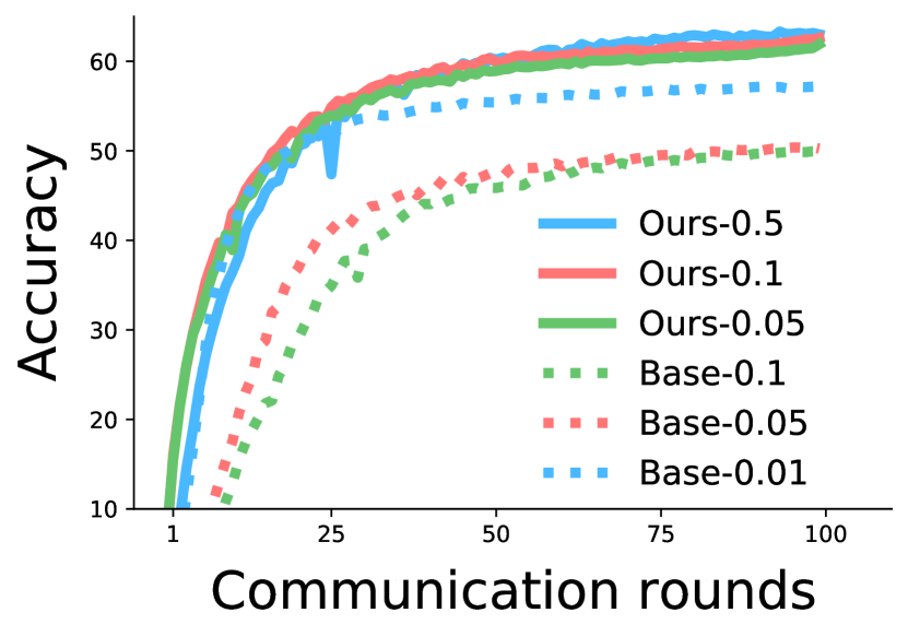
Figure 4: The impact of different learning rates for “FedNova” and “FedNova  +  SphereFed”. After applying SphereFed, training becomes more robust to different learning rates.

Table 4: Ablation study for FFC. Both CCVR and FFC methods exhibit performance gain on non-i.i.d. data. For sanity check, we collect local train sets to fine-tune the classifier. FFC is able to achieve a larger accuracy improvement than CCVR with significantly less communication and computation overheads (Tab. 1).

Calibration	IID	$\bm{\alpha=0.1}$
W/o	65.07	61.66
CCVR	65.03 ($\downarrow$ 0.04)	62.09 ($\uparrow$ 0.43)
FFC	65.15 ($\uparrow$ 0.08)	62.61 ($\uparrow$ 0.95)
Sanity check	65.17 ($\uparrow$ 0.10)	62.64 ($\uparrow$ 0.98)

How beneficial is FFC? In this set of experiments, we investigate how the closed-form classifier calibration (i.e., FFC) improves test accuracy. We apply CCVR and FFC individually for the classifier of SENet on CIFAR-100 after federated learning with “FedOpt  +  SphereFed”. As a sanity check, we collect all local train sets to fine-tune the classifier only. To ensure the sanity check truly reveals the upper bound of classifier calibration, we experiment different loss functions (i.e., CE and MSE) and learning rates for the sanity fine-tuning and report the best results we get. It can be seen from Fig. 4 that both CCVR and FFC achieve performance gains on non-i.i.d. data while FFC is able to improve accuracy more. CCVR estimates a GMM distribution for each class’s features and sample virtual features for model fine-tuning on the server. However, such a class-wise method has relatively high communication and computation complexities (which scale linearly with number of classes). Moreover, GMMs of different classes could be less separable when the number of classes increases, thereby further limiting its effectiveness. In contrast, FFC, with provable formulations, is agnostic to number of classes and more suitable for realistic many-class federated learning tasks [25, 81]. It is expected that FFC obtains comparable results as the sanity check because solving a linear classifier with either closed-form equations or SGD will converge to similar optimums [9, 61].

5.4 Efficient Communication and Computation

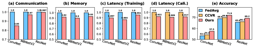
Figure 5: Efficiency comparison measured on a neural network accelerator [78, 91] with three models and CIFAR-100. (a) The normalized total communication amount. (b) The normalized peak memory consumption during local training. (c) The normalized latency for one-round local training. (d) The normalized latency for classifier calibration. (e) The test accuracy.

Besides accuracy gain, Hyperspherical Federated Learning also brings communication and computation savings depending on the size of classifier.

In Tab. 1, we compare the communication and computation costs related to the classifier for FedAvg, CCVR and our methods on MobileNetV2 and CIFAR-100. As seen in Tab. 1, SphereFed eliminates the need of updating and communicating (neither uploading nor downloading), resulting over two orders of magnitude communication and computation savings compared to FedAvg and CCVR. Figure 5 depicts the relative computational savings of different approaches during the federated training process, measured on a DNN training accelerator built on Xilinx VC707 FPGA evaluation board [78, 91]. Detailed settings about the DNN training accelerator are described in the appendix. SphereFed enables us to skip gradient computing for the classifier and thus to release some intermediate tensors used by gradient computing earlier. Overall, SphereFed achieves up to 10.5% and 13.6% savings on memory consumption and processing latency compared with FedAvg, respectively. SphereFed achieves a greater saving of training latency on MobileNetV2 than ConvNet and ResNet. This is because the computation workload associated with the convolutaional layers are smaller in MobileNetV2 due to the usage of the depthwise separable operations [62], leading to a greater relative savings when the classifier is skipped during the local training. We also measure the latency of classifier calibration using CCVR and our Fast Federated Calibration in Fig. 5 (d). Since calibration-related computation happens on both clients and the server, the reported latency consists of both the average latency on one client and the on-server latency. Our closed-form calibration saves up to 9.1% latency against CCVR and this efficiency improvement will be more pronounced when number of classes increases as analysed above.

6 Conclusions

We presented the Hyperspherical Federated Learning (SphereFed) framework to address the non-i.i.d. issue. The proposed method focuses on the pre-learning phase and complementary to existing federated learning methods. The hyperspherical representation is learned using an orthonormal basis of the weights of the frozen classifiers and the classifiers are calibrated post training. We show that a mean squared loss is more suitable to hyperspherical representation as opposed to cross-entropy due to the scaling issues. A Fast Federated Calibration (FFC) approach is proposed based on the mean squared loss. Extensive experiments indicate that SphereFed improves multiple existing federated learning algorithms by a considerable margin.

Appendix 0.A Extra Federated Learning Results

In this section, we present additional results under various system and training settings to further evaluate the robustness of our approach.

0.A.1 Different Local Training Epochs

Tuning the number of local epochs affects accuracy-communication trade-off for most federated learning algorithms. Prior studies [32, 51, 60] attempt to reduce the number of local training epochs to mitigate the disparity of local models. The default number of local training epochs is set as $E=10$ in the main manuscript. We further test different numbers of local training epochs $E=\{1,5\}$ in Tab. 5. When $E$ is set as 1, we increase the total number of rounds to 500 to ensure convergence. As is seen from Tab. 5, our method consistently improves the base algorithms with various numbers of local training epochs.

Table 5: Accuracy (%) with different number of local training epochs.

           Model            Method            $\bm{E=1}$            $\bm{E=5}$            MobileNetV2      (${\alpha=0.5}$)      FedAvg      70.51      68.40       +  CCVR      71.33  ($\uparrow$ 0.82)      68.93  ($\uparrow$ 0.53)       +  BABU      71.46  ($\uparrow$ 0.95)      69.10  ($\uparrow$ 0.70)       +   Ours      73.26  ($\uparrow$ 2.75)      72.02  ($\uparrow$ 3.62)            VGG13      (${\alpha=0.1}$)       FedNova      60.53      57.46       +  CCVR      61.31  ($\uparrow$ 0.78)      57.77  ($\uparrow$ 0.31)       +  BABU      62.75  ($\uparrow$ 2.22)      58.50  ($\uparrow$ 1.04)       +   Ours      64.75  ($\uparrow$ 4.22)      62.06  ($\uparrow$ 4.60)

0.A.2 Different Client Numbers

The default number of clients $K$ is set as 10 following prior work [41, 48]. We further test the performance of our methods when the system contains more clients. In Tab. 6, we partition CIFAR-100 training set to $K=100$ clients according to a Dirichlet distribution with a concentration parameter $\alpha=0.5$. During federated training, the central server randomly selects 10% clients to participate each round [32, 43, 54, 60]. For each method, we set the number of rounds as 500. According to results in Tab. 6,

Table 6: Accuracy (%) with $K=100$ clients.

Model Method Accuracy Model Method Accuracy MobileNetV2 FedAvg 68.26 VGG13 FedNova 49.04 +  CCVR 69.20  ($\uparrow$ 0.94) +  CCVR 50.45  ($\uparrow$ 1.41) +  BABU 69.14  ($\uparrow$ 0.88) +  BABU 51.27  ($\uparrow$ 2.23) +   Ours 71.38  ($\uparrow$ 5.12) +   Ours 55.23  ($\uparrow$ 6.19)

0.A.3 Different Learning Rate Scheduling Strategies

Besides adjusting the learning rate at each round according to a cosine annealing schedule, we further experiment another widely used learning rate scheduling strategy (e.g., multi-step scheduling) to verify the robustness of our approaches. Specifically, we decay the learning rate by $0.1$ every $40$ epochs. Empirical results in Tab. 7 indicate that our methods are able to bring state-of-the-art accuracy gain with different learning rate scheduling strategies.

Table 7: Accuracy (%) with different learning rate (LR) schedulings.

LR method Accuracy LR Method Accuracy Cosine FedAvg 68.78 Multi-step FedAvg 68.60 +  CCVR 69.14  ($\uparrow$ 0.36) +  CCVR 69.05  ($\uparrow$ 0.45) +  BABU 69.35  ($\uparrow$ 0.57) +  BABU 69.43  ($\uparrow$ 0.83) +   Ours 71.85  ($\uparrow$ 3.07) +   Ours 71.06  ($\uparrow$ 2.46)

Appendix 0.B Personalization Performance Comparison

We investigate the performance gain brought by SphereFed for personalized federated learning. Following the setup in [29, 54, 77], we first combine the training and testing sets of CIFAR-100 to a single dataset which contains 60,000 samples in total. Then, the combined dataset is partitioned into 10 clients according to a Dirichlet distribution with a concentration parameter $\alpha$. On each client, we use $15\%$ its local data as local testing set and the other as local training set. Each personalized local model is evaluated on its corresponding local testing set. The overall performance of personalized federated learning is evaluated by calculating the mean and standard deviation of local testing accuracies across all clients [29, 54, 77].

We consider four recent personalized federated learning baselines for comparison in Tab. 8. For instance, LG-FedAvg [44] jointly updates feature extractors and classifiers during local training and only aggregates classifiers on the server in order to learn compact local representations. In FedRep [15], local feature extractors and classifiers are updated sequentially and the servers aggregates updated feature extractors at each round. The state-of-the-art pFL method, BABU [54], is also included in the comparison.

For our methods, we use SphereFed during federated training. Since it is not necessary to get the optimal global classifier for pFL, we skip the FFC for the global classifier. Instead, we keep the learnt global feature extractor fixed and conduct personalization fine-tuning for the local classifier on each client. We consider two manners for the personalization fine-tunings. The first manner (duded ‘Ours (SGD)’ in Tab. 8) is to optimize the classifier on the local training set with SGD optimizer like prior arts [29, 54, 77]. The second manner (duded ‘Ours (FFC)’ in Tab. 8) is to adapt our FFC to compute the closed-form optimal classifier on the local training set (according to Eq. 7).

Empirical results in Tab. 8 indicate that our proposed methods are able to improve pFL as well with hyperspherical features which are better aligned and less biased.

Table 8: Accuracy (%) comparison of different personalized federated learning (pFL) methods. The numbers ‘A $\pm$ B’ are the ‘mean $\pm$ standard deviation’ of personalized accuracies across clients.

Data	FedAvg	LG-FedAvg	FedRep	BABU	Ours (FFC)	Ours (SGD)
$\bm{\alpha=0.5}$	$69.95\pm 3.96$	$71.67\pm 4.33$	$62.39\pm 3.91$	$72.34\pm 3.84$	$75.63\pm 3.13$	75.71$\pm$3.32
$\bm{\alpha=0.1}$	$80.16\pm 3.77$	$81.95\pm 3.69$	$73.63\pm 3.74$	$82.12\pm 3.63$	$84.06\pm 3.10$	84.12$\pm$3.29

Appendix 0.C Extra Calibration Results

0.C.1 Adapting An $\ell_{2}$ Penalty in the Closed-Form Solution

In Sec. 4.3, we formulate the calibrating the classifier ${\mathbf{W}}$ as a least square problem in Eq. 6. Theoretically, an $\ell_{2}$ penalty of ${\mathbf{W}}$ can be added and the objective of calibrating the classifier is,

$$\scalebox{0.85}{$\operatorname*{arg\,min}_{\mathbf{W}}\ \mathbb{E}_{({\mathbf{x}},y)\sim\mathcal{D}}\left[\mathcal{L}_{\textrm{{\tiny MSE}}}\left({\mathbf{W}}{\mathbf{z}},\ y\right)\right]+\lambda\|{\mathbf{W}}\|^{2}_{2}$ }~{},$$ (11)

where $\lambda$ is a hyper-parameter used to control the penalty intensity. As a result, the closed-form weights optimum (i.e., Eq. 10) becomes,

$$\scalebox{0.85}{${\mathbf{W}}^{*}=\left(\sum_{k=1}^{K}{\mathbf{V}}^{k}+\lambda{\mathbf{I}}\right)^{-1}\left(\sum_{k=1}^{K}{\mathbf{U}}^{k}\right)$ },$$ (12)

where ${\mathbf{I}}\in\mathbb{R}^{l\times l}$ is the identity matrix. In practise, we test different values for $\lambda\in\{0,\ 10^{-3},\ 10^{-2},\ 10^{-1},\ 10^{0},\ 10^{1}\}$ and find that the difference among resulted accuracies is less than 0.27% ($10^{-1}$ results in the better accuracy 71.96%). Therefore, we keep $\lambda=0$ in our main experiments.

0.C.2 Calibrate Weights One or Multiple Times?

Theoretically, we can conduct the Fast Federated Calibration (FFC) multiple times during the federated training. In practise, we attempt to calibrate the classifier every 10 rounds and get a final accuracy 71.88% which is quite close to the accuracy of one-time calibration (71.85%). This empirical result suggests that the pre-defined orthogonal hyperspherical ${\mathbf{W}}$ serves as a high-quality feature learning target (as discussed in Sec. 4.1) against a calibrated one. Moreover, conducting calibration multiple times will introduce extra communication and computation overheads. In this regard, we conduct FFC once after federated training in our main experiments.

0.C.3 Applying FFC with Features Trained with CE

The derivation of Fast Federated Calibration (FFC) relies on the mean square error (MSE) loss. However, in this section, we show that FFC can be used upon features trained by other losses (e.g., cross entropy loss) because the training of the feature extractor and the calibration of the classifier are decoupled. In addition, both CE and MSE have similar optimization goal, i.e., encouraging the feature extractor to make features of the $i$-th class close to ${\mathbf{w}}_{i}$. For instance, we train the feature extractor with cross entropy loss (CE) and then calibrate the classifier with our proposed FFC in Tab. 9. Experiential results verify that FFC is able to improve the classifier on features trained with CE.

Table 9: Applying FFC for the classifier on features trained with CE.

	FedAvg	+  Fix (R)	+  Fix (R) +  FFC
CE	63.90	64.91 ($\uparrow$ 1.01)	65.36 ($\uparrow$ 1.46)

Appendix 0.D Different Ways to Generate Orthogonal Classifier Initialization

We experiment two representative methods to generate the row-orthogonal weight matrix for classifier’s weight initialization.

• QR-decomposition method. In linear algebra, a QR decomposition is to decompose a random matrix ${\mathbf{A}}$ into a product ${\mathbf{A}}={\mathbf{Q}}{\mathbf{R}}$ of an orthogonal matrix ${\mathbf{Q}}$ and an upper triangular matrix ${\mathbf{R}}$ [1, 58, 73], in which ${\mathbf{Q}}$ is the matrix of our interest.

• Tammes method. To distribute $C$ two-dimensional vectors on an unit circle as uniformly as possible, one can randomly place the first vector and then put the next vector by shifting the previous vector for an angle of $\frac{2\pi}{C}$. However, when the dimension is larger than two, no such optimal separation algorithm exists, which is known as the Tammes problem [71]. To maximize the separation for any vector dimension, Mettes et al. [52] optimize an objective which encourages large cosine similarity of any pair of vectors with gradient decent. Following [52], we learn the vectors using SGD optimizer with $0.1$ learning rate and 0.9 momentum for $10^{4}$ steps.

Table 10: Accuracy (%) of different initialization methods for the classifier.

FedAvg+SphereFed (MobileNetv2 on CIFAR-100)	Init.	Rep. dim. ($l$)	#Classes ($C$)	Time	Accuracy
	QR	1280	100	0.02 s	71.85
	Tammes	1280	100	13.1 s	71.36

Tab. 10 shows the comparison of above two kinds of initialization methods for the orthogonal classifier weight matrix. QR-decomposition initialization achieves slightly better accuracy than the Tammes initialization. We also provide the wall time of the two methods which is measured on the machine with one NVIDIA GeForce GTX 1080 Ti GPU.

In all the other experiments of this work, QR method is used for SphereFed due to its efficiency and effectiveness.

Appendix 0.E Details of Hardware Experiments

We evaluate the hardware performance of different on an embedded DNN training accelerator [91] based on the Xilinx VC707 FPGA evaluation board [78]. A 32 by 64 systolic array is used to perform the tensor operations during the forward and backpropagation. Each systolic cell consists of a Multiply-Accumulate (MAC) unit which can perform a floating-point multiplication and addition within a clock cycle, and a special unit is implemented to perform the operations for the rest layers (e.g., group/batch normalization, ReLU). The hardware system runs at 100 MHz.

Appendix 0.F Details of Implementation

0.F.1 Model Architectures

We provide the detailed information of ConvNet, MobileNetV2, ResNet18, VGG13 and SENet18 in Tabs. 11, 14, 15, 12 and 13. For the ‘NormLayer’ after each convolution layer, two kinds of normalization layers are experimented. For experiments with MobileNetV2 and CIFAR-100, we instance the normalization layer as batch normalization. For other experiments, we use group normalization following prior arts [32, 43, 48, 66, 76, 84, 87].

0.F.2 Hyper-parameters

SphereFed and FFC do not introduce any extra hyper-parameter to base federated learning algorithms. Since we change the loss function from cross entropy to mean square error and these two loss functions have different magnitude, we tune the learning rate for both baselines and our methods using grid search from the limited candidate set $\{0.005,0.01,0.05,0.1,0.5,0.8,1.0\}$. Detailed default hyper-parameters are summarized in Tab. 16.

Table 11: Architecture of ConvNet

Block	Layers	Repetition
	Conv(3, 32, k=3, s=1), NormLayer(32), ReLU()	1
	Conv(32, 64, k=3, s=2), NormLayer(64), ReLU()	1
	Conv(64, 64, k=3, s=2), NormLayer(64), ReLU()	1
	Conv(64, 64, k=3, s=1), NormLayer(64), ReLU()	1
	Conv(64, 128, k=3, s=2), NormLayer(128), ReLU()	1
	Conv(128, 128, k=3, s=1), NormLayer(128), ReLU()	1
	Conv(128, 256, k=3, s=2), NormLayer(256), ReLU()	1
	Flatten()	1
	FeatureNorm() if use SphereFed	1
	FC(1024, 100, bias=False)	1

Table 12: Architecture of VGG13

Block	Layers	Repetition
	Conv(3, 64, k=3, s=1, p=1), NormLayer(64), ReLU()	1
	Conv(64, 64, k=3, s=1, p=1), NormLayer(64), ReLU()	1
	MaxPool2d(k=2, s=2)	1
	Conv(64, 128, k=3, s=1, p=1), NormLayer(128), ReLU()	1
	Conv(128, 128, k=3, s=1, p=1), NormLayer(128), ReLU()	1
	MaxPool2d(k=2, s=2)	1
	Conv(128, 256, k=3, s=1, p=1), NormLayer(256), ReLU()	1
	Conv(256, 256, k=3, s=1, p=1), NormLayer(256), ReLU()	1
	MaxPool2d(k=2, s=2)	1
	Conv(256, 512, k=3, s=1, p=1), NormLayer(256), ReLU()	1
	Conv(512, 512, k=3, s=1, p=1), NormLayer(256), ReLU()	1
	MaxPool2d(k=2, s=2)	1
	Conv(512, 512, k=3, s=1, p=1), NormLayer(256), ReLU()	2
	MaxPool2d(k=TIN_S, s=TIN_S)	1
	AvgPool2d(k=1, s=1)
	Flatten()	1
	FeatureNorm() if use SphereFed	1
	FC(512, 100, bias=False)	1
*: TIN_S=1 if dataset is CIFAR-100 and TIN_S=2 if dataset is TinyImageNet.

Table 13: Architecture of SENet18

Block	Layers	Repetition
	Conv(3, 64, k=3, s=1, p=1), NormLayer(64), ReLU()	1
B1	Conv(64, 64, k=3, s=TIN_S, p=1), NormLayer(64), ReLU() Conv(64, 64, k=3, s=1, p=1), NormLayer(64), ReLU() SquzzeExcitationModule()	1
	Conv(64, 64, k=3, s=1, p=1), NormLayer(64), ReLU() Conv(64, 64, k=3, s=1, p=1), NormLayer(64), ReLU() SquzzeExcitationModule()	1
B2	Conv(64, 128, k=3, s=2, p=1), NormLayer(128), ReLU() Conv(128, 128, k=3, s=1, p=1), NormLayer(128), ReLU() SquzzeExcitationModule()	1
	Conv(128, 128, k=3, s=1, p=1), NormLayer(128), ReLU() Conv(128, 128, k=3, s=1, p=1), NormLayer(128), ReLU() SquzzeExcitationModule()	1
B3	Conv(128, 256, k=3, s=2, p=1), NormLayer(256), ReLU() Conv(256, 256, k=3, s=1, p=1), NormLayer(256), ReLU() SquzzeExcitationModule()	1
	Conv(256, 256, k=3, s=1, p=1), NormLayer(256), ReLU() Conv(256, 256, k=3, s=1, p=1), NormLayer(256), ReLU() SquzzeExcitationModule()	1
B4	Conv(256, 512, k=3, s=2, p=1), NormLayer(512), ReLU() Conv(512, 512, k=3, s=1, p=1), NormLayer(256), ReLU() SquzzeExcitationModule()	1
	Conv(512, 512, k=3, s=1, p=1), NormLayer(512), ReLU() Conv(512, 512, k=3, s=1, p=1), NormLayer(512), ReLU() SquzzeExcitationModule()	1
	AvgPool2d(k=4, s=4)	1
	Flatten()	1
	FeatureNorm() if use SphereFed	1
	FC(512, 100, bias=False)	1
*: TIN_S=1 if dataset is CIFAR-100 and TIN_S=2 if dataset is TinyImageNet.

Table 14: Architecture of MobileNetV2.

Block	Layers	Repetition
	Conv(3, 32, k=3, s=1), NormLayer(32), ReLU()	1
B1	Conv(32, 32, k=1, s=1), NormLayer(32), ReLU() Conv(32, 32, k=3, s=1, p=1, g=32), NormLayer(32), ReLU() Conv(32, 16, k=1, s=1), NormLayer(16), ReLU()	1
B2	Conv(16, 96, k=1, s=1), NormLayer(96), ReLU() Conv(96, 96, k=3, s=TIN_S, p=1, g=96), NormLayer(96), ReLU() Conv(96, 24, k=1, s=1), NormLayer(24), ReLU()	1
	Conv(24, 144, k=1, s=1), NormLayer(144), ReLU() Conv(144, 144, k=3, s=1, p=1, g=144), NormLayer(144), ReLU() Conv(144, 24, k=1, s=1), NormLayer(24), ReLU()	1
B3	Conv(24, 144, k=1, s=1), NormLayer(144), ReLU() Conv(144, 144, k=3, s=2, p=1, g=144), NormLayer(144), ReLU() Conv(144, 32, k=1, s=1), NormLayer(32), ReLU()	1
	Conv(32, 192, k=1, s=1), NormLayer(192), ReLU() Conv(192, 192, k=3, s=1, p=1, g=192), NormLayer(192), ReLU() Conv(192, 32, k=1, s=1), NormLayer(32), ReLU()	2
B4	Conv(32, 192, k=1, s=1), NormLayer(192), ReLU() Conv(192, 192, k=3, s=2, p=1, g=192), NormLayer(192), ReLU() Conv(192, 64, k=1, s=1), NormLayer(64), ReLU()	1
	Conv(64, 384, k=1, s=1), NormLayer(384), ReLU() Conv(384, 384, k=3, s=1, p=1, g=384), NormLayer(384), ReLU() Conv(384, 64, k=1, s=1), NormLayer(64), ReLU()	3
B5	Conv(64, 384, k=1, s=1), NormLayer(384), ReLU() Conv(384, 384, k=3, s=1, p=1, g=384), NormLayer(384), ReLU() Conv(384, 96, k=1, s=1), NormLayer(96), ReLU()	1
	Conv(96, 576, k=1, s=1), NormLayer(576), ReLU() Conv(576, 576, k=3, s=1, p=1, g=576), NormLayer(576), ReLU() Conv(576, 96, k=1, s=1), NormLayer(96), ReLU()	2
B6	Conv(96, 576, k=1, s=1), NormLayer(576), ReLU() Conv(576, 576, k=3, s=2, p=1, g=576), NormLayer(576), ReLU() Conv(576, 160, k=1, s=1), NormLayer(160), ReLU()	1
	Conv(160, 960, k=1, s=1), NormLayer(960), ReLU() Conv(960, 960, k=3, s=1, p=1, g=960), NormLayer(960), ReLU() Conv(960, 160, k=1, s=1), NormLayer(160), ReLU()	2
B7	Conv(160, 960, k=1, s=1), NormLayer(960), ReLU() Conv(960, 960, k=3, s=1, p=1, g=960), NormLayer(960), ReLU() Conv(960, 320, k=1, s=1), NormLayer(320), ReLU()	1
	Conv(320, 1280, k=1, s=1), NormLayer(1280), ReLU()	1
	AvgPool2d(k=4, s=4)	1
	Flatten()	1
	FeatureNorm() if use SphereFed	1
	FC(1280, 100, bias=False)	1
*: TIN_S=1 if dataset is CIFAR-100 and TIN_S=2 if dataset is TinyImageNet.

Table 15: Architecture of ResNet18

Block	Layers	Repetition
	Conv(3, 64, k=3, s=1, p=1), NormLayer(64), ReLU()	1
B1	Conv(64, 64, k=3, s=TIN_S, p=1), NormLayer(64), ReLU() Conv(64, 64, k=3, s=1, p=1), NormLayer(64), ReLU()	1
	Conv(64, 64, k=3, s=1, p=1), NormLayer(64), ReLU() Conv(64, 64, k=3, s=1, p=1), NormLayer(64), ReLU()	1
B2	Conv(64, 128, k=3, s=2, p=1), NormLayer(128), ReLU() Conv(128, 128, k=3, s=1, p=1), NormLayer(128), ReLU()	1
	Conv(128, 128, k=3, s=1, p=1), NormLayer(128), ReLU() Conv(128, 128, k=3, s=1, p=1), NormLayer(128), ReLU()	1
B3	Conv(128, 256, k=3, s=2, p=1), NormLayer(256), ReLU() Conv(256, 256, k=3, s=1, p=1), NormLayer(256), ReLU()	1
	Conv(256, 256, k=3, s=1, p=1), NormLayer(256), ReLU() Conv(256, 256, k=3, s=1, p=1), NormLayer(256), ReLU()	1
B4	Conv(256, 512, k=3, s=2, p=1), NormLayer(512), ReLU() Conv(512, 512, k=3, s=1, p=1), NormLayer(256), ReLU()	1
	Conv(512, 512, k=3, s=1, p=1), NormLayer(512), ReLU() Conv(512, 512, k=3, s=1, p=1), NormLayer(512), ReLU()	1
	AvgPool2d(k=4, s=4)	1
	Flatten()	1
	FeatureNorm() if use SphereFed	1
	FC(512, 100, bias=False)	1
*: TIN_S=1 if dataset is CIFAR-100 and TIN_S=2 if dataset is TinyImageNet.

Table 16: Summary of default hyper-parameters.

Method	Hyper-parameters	IID	$\bm{\alpha=0.5}$	$\bm{\alpha=0.1}$	TinyImageNet
FedAvg (MobileNetV2)	Rounds	100
	Optimizer	SGD
	Weights decay	0.00001
	Momentum	0.9
	Local epochs	10
	Local batch size	64
	Learning rate	0.1
+  CCVR	# virtual features per class [48]	500	500	500	1000
	fine-tuning learning rate [48]	0.00001	0.00001	0.00001	0.00001
+  BABU	learning rate	0.1	0.1	0.1	0.01
+  Ours	learning rate	0.5	0.5	1.0	0.5
FedProx (ResNet18)	Rounds	100
	Optimizer	SGD
	Weights decay	0.00001
	Momentum	0.9
	Local epochs	10
	Local batch size	64
	Learning rate	0.1
	$\mu$	0.001
+  CCVR	# virtual features per class [48]	500	500	500	1000
	fine-tuning learning rate [48]	0.00001	0.00001	0.00001	0.00001
+  BABU	learning rate	0.1	0.1	0.1	0.1
	$\mu$	0.001	0.001	0.001	0.001
+  Ours	learning rate	0.5	0.5	0.5	0.5
	$\mu$	0.0001	0.0001	0.0001	0.001
FedNova (VGG13)	Rounds	100
	Optimizer	SGD
	Weights decay	0.00001
	Momentum	0.9
	Local epochs	10
	Local batch size	64
	Learning rate	0.01
+  CCVR	# virtual features per class [48]	500	500	500	1000
	fine-tuning learning rate [48]	0.00001	0.00001	0.00001	0.00001
+  BABU	learning rate	0.01	0.01	0.01	0.001
+  Ours	learning rate	0.1	0.1	0.1	0.1
FedOpt (SENet18)	Rounds	100
	Optimizer	SGD
	Weights decay	0.00001
	Momentum	0.9
	Local epochs	10
	Local batch size	64
	Local learning rate	0.01
	On-server optimizer [60]	SGD
	On-server learning rate [60]	1.0
	On-server momentum [60]	0.3
+  CCVR	# virtual features per class [48]	500	500	500	1000
	fine-tuning learning rate [48]	0.00001	0.00001	0.00001	0.00001
+  BABU	Local learning rate	0.01	0.01	0.01	0.01
+  Ours	Local learning rate	0.5	0.5	0.5	0.5

References

- [1] Torch.linalg.qr¶, https://pytorch.org/docs/stable/generated/torch.linalg.qr.html
- [2] Acar, D.A.E., Zhao, Y., Matas, R., Mattina, M., Whatmough, P., Saligrama, V.: Federated learning based on dynamic regularization. In: International Conference on Learning Representations (2021), https://openreview.net/forum?id=B7v4QMR6Z9w
- [3] Acar, D.A.E., Zhao, Y., Zhu, R., Matas, R., Mattina, M., Whatmough, P., Saligrama, V.: Debiasing model updates for improving personalized federated training. In: International Conference on Machine Learning. pp. 21–31. PMLR (2021)
- [4] Achille, A., Golatkar, A., Ravichandran, A., Polito, M., Soatto, S.: Lqf: Linear quadratic fine-tuning. In: Proceedings of the IEEE/CVF Conference on Computer Vision and Pattern Recognition. pp. 15729–15739 (2021)
- [5] Al-Shedivat, M., Gillenwater, J., Xing, E., Rostamizadeh, A.: Federated learning via posterior averaging: A new perspective and practical algorithms. In: International Conference on Learning Representations (ICLR) (2021)
- [6] Anzai, Y.: Pattern recognition and machine learning. Elsevier (2012)
- [7] Arivazhagan, M.G., Aggarwal, V., Singh, A.K., Choudhary, S.: Federated learning with personalization layers. arXiv preprint arXiv:1912.00818 (2019)
- [8] Belkin, M.: Fit without fear: remarkable mathematical phenomena of deep learning through the prism of interpolation. arXiv preprint arXiv:2105.14368 (2021)
- [9] Boyd, S., Boyd, S.P., Vandenberghe, L.: Convex optimization. Cambridge university press (2004)
- [10] Brier, G.W., et al.: Verification of forecasts expressed in terms of probability. Monthly weather review 78(1), 1–3 (1950)
- [11] Bui, D., Malik, K., Goetz, J., Liu, H., Moon, S., Kumar, A., Shin, K.G.: Federated user representation learning. arXiv preprint arXiv:1909.12535 (2019)
- [12] Chen, C., Xu, H., Wang, W., Li, B., Li, B., Chen, L., Zhang, G.: Communication-efficient federated learning with adaptive parameter freezing. In: 2021 IEEE 41st International Conference on Distributed Computing Systems (ICDCS). pp. 1–11. IEEE (2021)
- [13] Chen, Y., Sun, X., Jin, Y.: Communication-efficient federated deep learning with layerwise asynchronous model update and temporally weighted aggregation. IEEE transactions on neural networks and learning systems 31(10), 4229–4238 (2019)
- [14] Cheraghian, A., Rahman, S., Fang, P., Roy, S.K., Petersson, L., Harandi, M.: Semantic-aware knowledge distillation for few-shot class-incremental learning. In: Proceedings of the IEEE/CVF Conference on Computer Vision and Pattern Recognition. pp. 2534–2543 (2021)
- [15] Collins, L., Hassani, H., Mokhtari, A., Shakkottai, S.: Exploiting shared representations for personalized federated learning. In: International Conference on Machine Learning. pp. 2089–2099. PMLR (2021)
- [16] Diao, E., Ding, J., Tarokh, V.: Heterofl: Computation and communication efficient federated learning for heterogeneous clients. International Conference on Learning Representations (2021)
- [17] Dong, X., Yin, H., Alvarez, J.M., Kautz, J., Molchanov, P.: Deep neural networks are surprisingly reversible: A baseline for zero-shot inversion. arXiv preprint arXiv:2107.06304 (2021)
- [18] Duan, J.H., Li, W., Lu, S.: Feddna: Federated learning with decoupled normalization-layer aggregation for non-iid data. In: Joint European Conference on Machine Learning and Knowledge Discovery in Databases. pp. 722–737. Springer (2021)
- [19] Golik, P., Doetsch, P., Ney, H.: Cross-entropy vs. squared error training: a theoretical and experimental comparison. In: Interspeech. vol. 13, pp. 1756–1760 (2013)
- [20] He, C., Li, S., So, J., Zhang, M., Wang, H., Wang, X., Vepakomma, P., Singh, A., Qiu, H., Shen, L., Zhao, P., Kang, Y., Liu, Y., Raskar, R., Yang, Q., Annavaram, M., Avestimehr, S.: Fedml: A research library and benchmark for federated machine learning. arXiv preprint arXiv:2007.13518 (2020)
- [21] He, K., Zhang, X., Ren, S., Sun, J.: Delving deep into rectifiers: Surpassing human-level performance on imagenet classification. In: Proceedings of the IEEE international conference on computer vision. pp. 1026–1034 (2015)
- [22] He, K., Zhang, X., Ren, S., Sun, J.: Deep residual learning for image recognition. In: Proceedings of the IEEE conference on computer vision and pattern recognition. pp. 770–778 (2016)
- [23] Hoffer, E., Hubara, I., Soudry, D.: Fix your classifier: the marginal value of training the last weight layer. International Conference on Learning Representations (2018)
- [24] Hsu, T.M.H., Qi, H., Brown, M.: Measuring the effects of non-identical data distribution for federated visual classification. arXiv preprint arXiv:1909.06335 (2019)
- [25] Hsu, T.M.H., Qi, H., Brown, M.: Federated visual classification with real-world data distribution. In: European Conference on Computer Vision. pp. 76–92. Springer (2020)
- [26] Hu, J., Shen, L., Sun, G.: Squeeze-and-excitation networks. In: Proceedings of the IEEE conference on computer vision and pattern recognition. pp. 7132–7141 (2018)
- [27] Hui, L., Belkin, M.: Evaluation of neural architectures trained with square loss vs cross-entropy in classification tasks. ICLR (2020)
- [28] Jain, V., Learned-Miller, E.: Online domain adaptation of a pre-trained cascade of classifiers. In: CVPR 2011. pp. 577–584. IEEE (2011)
- [29] Jiang, Y., Konečnỳ, J., Rush, K., Kannan, S.: Improving federated learning personalization via model agnostic meta learning. arXiv preprint arXiv:1909.12488 (2019)
- [30] Kairouz, P., McMahan, H.B., Avent, B., Bellet, A., Bennis, M., Bhagoji, A.N., Bonawitz, K., Charles, Z., Cormode, G., Cummings, R., et al.: Advances and open problems in federated learning. arXiv preprint arXiv:1912.04977 (2019)
- [31] Kang, B., Xie, S., Rohrbach, M., Yan, Z., Gordo, A., Feng, J., Kalantidis, Y.: Decoupling representation and classifier for long-tailed recognition. International Conference on Learning Representations (2020)
- [32] Karimireddy, S.P., Kale, S., Mohri, M., Reddi, S., Stich, S., Suresh, A.T.: Scaffold: Stochastic controlled averaging for federated learning. In: International Conference on Machine Learning. pp. 5132–5143. PMLR (2020)
- [33] Khosla, P., Teterwak, P., Wang, C., Sarna, A., Tian, Y., Isola, P., Maschinot, A., Liu, C., Krishnan, D.: Supervised contrastive learning. Advances in Neural Information Processing Systems 33, 18661–18673 (2020)
- [34] Kornblith, S., Chen, T., Lee, H., Norouzi, M.: Why do better loss functions lead to less transferable features? Advances in Neural Information Processing Systems 34 (2021)
- [35] Krizhevsky, A.: Learning multiple layers of features from tiny images. Tech. rep. (2009)
- [36] Kuangliu: Pytorch-cifar/vgg.py, https://github.com/kuangliu/pytorch-cifar/blob/master/models/vgg.py
- [37] Le, Y., Yang, X.S.: Tiny imagenet visual recognition challenge (2015)
- [38] Lezama, J., Qiu, Q., Musé, P., Sapiro, G.: Ole: Orthogonal low-rank embedding-a plug and play geometric loss for deep learning. In: Proceedings of the IEEE Conference on Computer Vision and Pattern Recognition. pp. 8109–8118 (2018)
- [39] Li, D., Wang, J.: Fedmd: Heterogenous federated learning via model distillation. NeurIPS 2019 Workshop on Federated Learning for Data Privacy and Confidentiality (2019)
- [40] Li, Q., Diao, Y., Chen, Q., He, B.: Federated learning on non-iid data silos: An experimental study. IEEE International Conference on Data Engineering (2021)
- [41] Li, Q., He, B., Song, D.: Model-contrastive federated learning. In: Proceedings of the IEEE/CVF Conference on Computer Vision and Pattern Recognition. pp. 10713–10722 (2021)
- [42] Li, T., Sahu, A.K., Talwalkar, A., Smith, V.: Federated learning: Challenges, methods, and future directions. IEEE Signal Processing Magazine 37(3), 50–60 (2020)
- [43] Li, T., Sahu, A.K., Zaheer, M., Sanjabi, M., Talwalkar, A., Smith, V.: Federated optimization in heterogeneous networks. Proceedings of Machine Learning and Systems 2, 429–450 (2020)
- [44] Liang, P.P., Liu, T., Ziyin, L., Allen, N.B., Auerbach, R.P., Brent, D., Salakhutdinov, R., Morency, L.P.: Think locally, act globally: Federated learning with local and global representations. arXiv preprint arXiv:2001.01523 (2020)
- [45] Liu, W., Wen, Y., Yu, Z., Li, M., Raj, B., Song, L.: Sphereface: Deep hypersphere embedding for face recognition. In: Proceedings of the IEEE conference on computer vision and pattern recognition. pp. 212–220 (2017)
- [46] Liu, X., Tang, Z., Huang, H., Zhang, T., Yang, B.: Multiple learning for regression in big data. In: 2019 18th IEEE International Conference On Machine Learning And Applications (ICMLA). pp. 587–594. IEEE (2019)
- [47] Loshchilov, I., Hutter, F.: Sgdr: Stochastic gradient descent with warm restarts. arXiv preprint arXiv:1608.03983 (2016)
- [48] Luo, M., Chen, F., Hu, D., Zhang, Y., Liang, J., Feng, J.: No fear of heterogeneity: Classifier calibration for federated learning with non-iid data. 35th Conference on Neural Information Processing Systems (2021)
- [49] van der Maaten, L., Hinton, G.: Visualizing data using t-sne. Journal of Machine Learning Research 9(86), 2579–2605 (2008), http://jmlr.org/papers/v9/vandermaaten08a.html
- [50] Mai, X., Liao, Z.: High dimensional classification via empirical risk minimization: Improvements and optimality. arXiv preprint arXiv:1905.13742 (2019)
- [51] McMahan, B., Moore, E., Ramage, D., Hampson, S., y Arcas, B.A.: Communication-efficient learning of deep networks from decentralized data. In: Artificial intelligence and statistics. pp. 1273–1282. PMLR (2017)
- [52] Mettes, P., van der Pol, E., Snoek, C.: Hyperspherical prototype networks. Advances in neural information processing systems 32 (2019)
- [53] Muthukumar, V., Narang, A., Subramanian, V., Belkin, M., Hsu, D., Sahai, A.: Classification vs regression in overparameterized regimes: Does the loss function matter? Journal of Machine Learning Research 22(222), 1–69 (2021)
- [54] Oh, J., Kim, S., Yun, S.Y.: Fedbabu: Towards enhanced representation for federated image classification. International Conference on Learning Representations (2021)
- [55] Oh, J., Yoo, H., Kim, C., Yun, S.Y.: Boil: Towards representation change for few-shot learning. International Conference on Learning Representations (2021)
- [56] Paszke, A., Gross, S., Massa, F., Lerer, A., Bradbury, J., Chanan, G., Killeen, T., Lin, Z., Gimelshein, N., Antiga, L., et al.: Pytorch: An imperative style, high-performance deep learning library. Advances in neural information processing systems 32 (2019)
- [57] Puigcerver, J., Riquelme, C., Mustafa, B., Renggli, C., Pinto, A.S., Gelly, S., Keysers, D., Houlsby, N.: Scalable transfer learning with expert models. International Conference on Learning Representations (2021)
- [58] Pursell, L., Trimble, S.: Gram-schmidt orthogonalization by gauss elimination. The American Mathematical Monthly 98(6), 544–549 (1991)
- [59] Raghu, A., Raghu, M., Bengio, S., Vinyals, O.: Rapid learning or feature reuse? towards understanding the effectiveness of maml. International Conference on Learning Representations (2019)
- [60] Reddi, S., Charles, Z., Zaheer, M., Garrett, Z., Rush, K., Konečnỳ, J., Kumar, S., McMahan, H.B.: Adaptive federated optimization. International Conference on Learning Representations (2021)
- [61] Saad, D.: Online algorithms and stochastic approximations. Online Learning 5, 6–3 (1998)
- [62] Sandler, M., Howard, A., Zhu, M., Zhmoginov, A., Chen, L.C.: Mobilenetv2: Inverted residuals and linear bottlenecks. In: Proceedings of the IEEE conference on computer vision and pattern recognition. pp. 4510–4520 (2018)
- [63] Sangari, A., Sethares, W.: Convergence analysis of two loss functions in soft-max regression. IEEE Transactions on Signal Processing 64(5), 1280–1288 (2015)
- [64] Shamir, O., Srebro, N., Zhang, T.: Communication-efficient distributed optimization using an approximate newton-type method. In: International conference on machine learning. pp. 1000–1008. PMLR (2014)
- [65] Shao, S., Xing, L., Wang, Y., Xu, R., Zhao, C., Wang, Y., Liu, B.: Mhfc: Multi-head feature collaboration for few-shot learning. In: Proceedings of the 29th ACM International Conference on Multimedia. pp. 4193–4201 (2021)
- [66] Shoham, N., Avidor, T., Keren, A., Israel, N., Benditkis, D., Mor-Yosef, L., Zeitak, I.: Overcoming forgetting in federated learning on non-iid data. NeurIPS 2019 Workshop on Federated Learning for Data Privacy and Confidentiality (2019)
- [67] Simonyan, K., Zisserman, A.: Very deep convolutional networks for large-scale image recognition. arXiv preprint arXiv:1409.1556 (2014)
- [68] Singhal, K., Sidahmed, H., Garrett, Z., Wu, S., Rush, J., Prakash, S.: Federated reconstruction: Partially local federated learning. Advances in Neural Information Processing Systems 34 (2021)
- [69] Smith, V., Chiang, C.K., Sanjabi, M., Talwalkar, A.S.: Federated multi-task learning. Advances in neural information processing systems 30 (2017)
- [70] Sun, B., Huo, H., Yang, Y., Bai, B.: Partialfed: Cross-domain personalized federated learning via partial initialization. Advances in Neural Information Processing Systems 34 (2021)
- [71] Tammes, P.M.L.: On the origin of number and arrangement of the places of exit on the surface of pollen-grains. Recueil des travaux botaniques néerlandais 27(1), 1–84 (1930)
- [72] Thrampoulidis, C., Oymak, S., Soltanolkotabi, M.: Theoretical insights into multiclass classification: A high-dimensional asymptotic view. Advances in Neural Information Processing Systems (2020)
- [73] Trefethen, L.N., Bau III, D.: Numerical linear algebra, vol. 50. Siam (1997)
- [74] Vaswani, A., Shazeer, N., Parmar, N., Uszkoreit, J., Jones, L., Gomez, A.N., Kaiser, Ł., Polosukhin, I.: Attention is all you need. In: Advances in neural information processing systems. pp. 5998–6008 (2017)
- [75] Venkat, N., Kundu, J.N., Singh, D., Revanur, A., et al.: Your classifier can secretly suffice multi-source domain adaptation. Advances in Neural Information Processing Systems 33, 4647–4659 (2020)
- [76] Wang, J., Liu, Q., Liang, H., Joshi, G., Poor, H.V.: Tackling the objective inconsistency problem in heterogeneous federated optimization. Advances in neural information processing systems (2020)
- [77] Wang, K., Mathews, R., Kiddon, C., Eichner, H., Beaufays, F., Ramage, D.: Federated evaluation of on-device personalization. arXiv preprint arXiv:1910.10252 (2019)
- [78] Xilinx: Xilinx virtex-7 fpga vc707 evaluation kit, https://www.xilinx.com/products/boards-and-kits/ek-v7-vc707-g.html
- [79] Xu, A., Huang, H.: Coordinating momenta for cross-silo federated learning. In: Proceedings of the AAAI Conference on Artificial Intelligence. vol. 36, pp. 8735–8743 (2022)
- [80] Xu, C., Hong, Z., Huang, M., Jiang, T.: Acceleration of federated learning with alleviated forgetting in local training. In: International Conference on Learning Representations (2021)
- [81] Yang, K., Fan, T., Chen, T., Shi, Y., Yang, Q.: A quasi-newton method based vertical federated learning framework for logistic regression. The 2nd International Workshop on Federated Learning for Data Privacy and Confidentiality, in Conjunction with NeurIPS 2019 (2019)
- [82] Yao, X., Sun, L.: Continual local training for better initialization of federated models. In: 2020 IEEE International Conference on Image Processing (ICIP). pp. 1736–1740. IEEE (2020)
- [83] Ye, H.J., Hu, H., Zhan, D.C.: Learning adaptive classifiers synthesis for generalized few-shot learning. International Journal of Computer Vision 129(6), 1930–1953 (2021)
- [84] Yoon, J., Jeong, W., Lee, G., Yang, E., Hwang, S.J.: Federated continual learning with weighted inter-client transfer. In: International Conference on Machine Learning. pp. 12073–12086. PMLR (2021)
- [85] Yoon, T., Shin, S., Hwang, S.J., Yang, E.: Fedmix: Approximation of mixup under mean augmented federated learning. International Conference on Learning Representations (2021)
- [86] You, K., Liu, Y., Wang, J., Long, M.: Logme: Practical assessment of pre-trained models for transfer learning. In: International Conference on Machine Learning. pp. 12133–12143. PMLR (2021)
- [87] Yuan, H., Zaheer, M., Reddi, S.: Federated composite optimization. In: International Conference on Machine Learning. pp. 12253–12266. PMLR (2021)
- [88] Zhai, A., Wu, H.Y.: Classification is a strong baseline for deep metric learning. arXiv preprint arXiv:1811.12649 (2018)
- [89] Zhang, L., Luo, Y., Bai, Y., Du, B., Duan, L.Y.: Federated learning for non-iid data via unified feature learning and optimization objective alignment. In: Proceedings of the IEEE/CVF International Conference on Computer Vision. pp. 4420–4428 (2021)
- [90] Zhang, S.Q., Lin, J., Zhang, Q.: A multi-agent reinforcement learning approach for efficient client selection in federated learning. arXiv preprint arXiv:2201.02932 (2022)
- [91] Zhang, S.Q., McDanel, B., Kung, H.: Fast: Dnn training under variable precision block floating point with stochastic rounding. International Symposium on High-Performance Computer Architecture (2021)
- [92] Zhang, T., Yang, B.: Box–cox transformation in big data. Technometrics 59(2), 189–201 (2017)
- [93] Zhao, N., Wu, Z., Lau, R.W., Lin, S.: What makes instance discrimination good for transfer learning? International Conference on Learning Representations (2021)
- [94] Zhao, Y., Li, M., Lai, L., Suda, N., Civin, D., Chandra, V.: Federated learning with non-iid data. arXiv preprint arXiv:1806.00582 (2018)
- [95] Zheng, Y., Pal, D.K., Savvides, M.: Ring loss: Convex feature normalization for face recognition. In: Proceedings of the IEEE conference on computer vision and pattern recognition. pp. 5089–5097 (2018)
- [96] Zhu, Y., Bai, Y., Wei, Y.: Spherical feature transform for deep metric learning. In: European Conference on Computer Vision. pp. 420–436. Springer (2020)
- [97] Zhu, Z., Hong, J., Zhou, J.: Data-free knowledge distillation for heterogeneous federated learning. In: International Conference on Machine Learning. pp. 12878–12889. PMLR (2021)