New high-precision strong lensing modeling of Abell 2744

We present a new strong lensing model of the Hubble Frontier Fields galaxy cluster Abell 2744, at $z=0.3072$, by exploiting archival Hubble Space Telescope (HST) multi-band imaging and Multi Unit Spectroscopic Explorer (MUSE) follow-up spectroscopy. The lens model considers 90 spectroscopically confirmed multiple images (from 30 background sources), which represents the largest secure sample for this cluster field prior to the recently acquired James Webb Space Telescope observations. The inclusion of the sub-structures within several extended sources as model constraints allows us to accurately characterize the inner total mass distribution of the cluster and the position of the cluster critical lines. We include the lensing contribution of 225 cluster members, 202 of which are spectroscopically confirmed. We complement this sample with 23 photometric member galaxies which are identified with a convolution neural network methodology with a high degree of purity. We also measure the internal velocity dispersion of 85 cluster galaxies, down to $m_{F160W}=22$, to independently estimate the role of the subhalo mass component in the lens model. We investigate the effect of the cluster environment on the total mass reconstruction of the cluster core with two different mass parameterizations. We consider the mass contribution from three external clumps, either based on previous weak-lensing studies, or extended HST imaging of luminous members around the cluster core. In the latter case, the observed positions of the multiple images are better reproduced, with a remarkable accuracy of $\sim 0.37\arcsec$, a factor of $\sim 2$ smaller than previous lens models, that exploited the same HST and MUSE data-sets. As part of this work, we develop and make publicly available a Strong Lensing Online Tool (SLOT) to exploit the predictive power and the full statistical information of this and future models, through a simple graphical interface. We plan to apply our new high-precision strong lensing model to the first analysis of the GLASS-JWST-ERS program, specifically to measure the intrinsic physical properties of high-$z$ galaxies from robust magnification maps.

1 Introduction

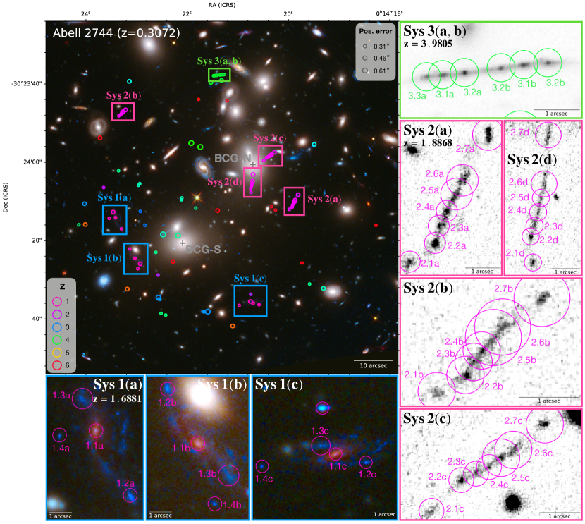
Figure 1: Color-composite RGB image of A2744 (credits: NASA/ESA). Circles show the positions of the 90 spectroscopically confirmed multiple images included in the SL model, color-coded according to their redshift value. The size of the circle illustrates the adopted (re-scaled) positional error in the modeling. Colored squares highlight the systems of multiple images for which additional lensed clumps have been identified. The two cluster BCGs (BCG-N and BCG-S) are labeled in gray.

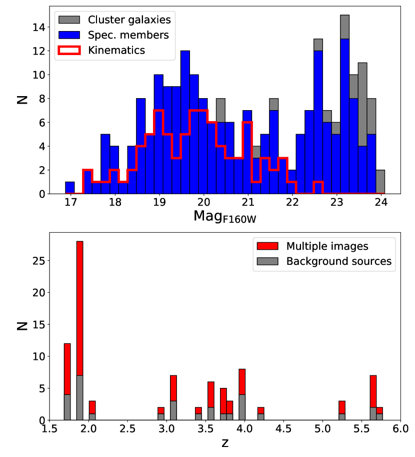
Figure 2: Top: Distribution of cluster member galaxies as a function of their magnitudes in the HST/F160W filter. The photometric sample of cluster members used in our lens model is plotted in gray, with the spectroscopic members pictured in blue. Cluster members with a reliable measurement of their internal stellar velocity dispersion are highlighted in red. Bottom: Redshift distribution of the observed 90 multiple images used to constrain the reference lens model described in this work.

Figure 3: Cumulative distributions of the distances of the multiple images from the Northern BCG (BCG-N) of A2744: in red the distribution of the images used as constraints in this work (90 multiple images in total) and in blue the images used in R21.

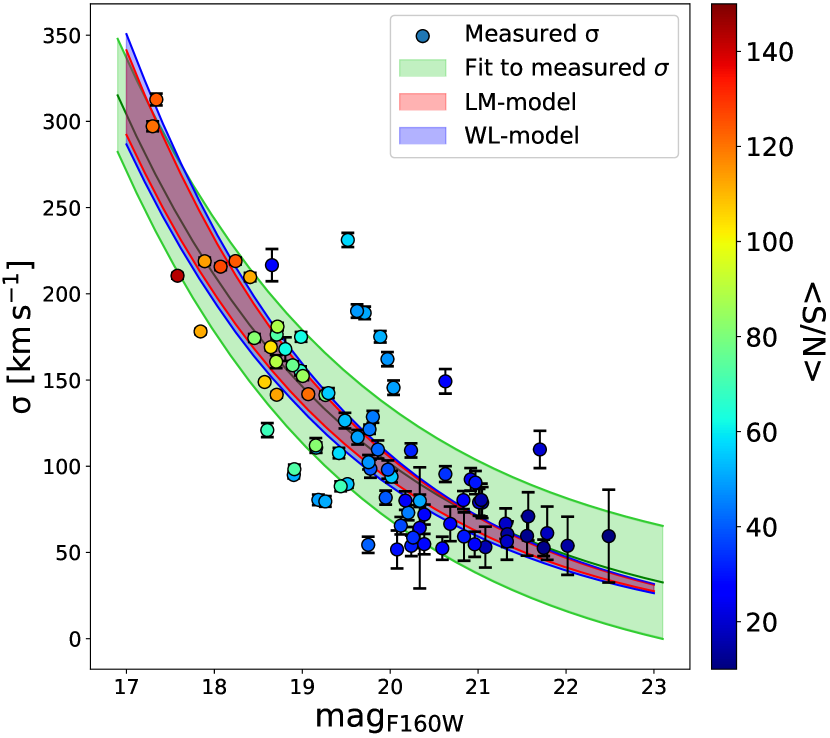
Figure 4: Measured internal stellar velocity dispersions of 85 cluster galaxies as a function of their magnitudes in the HST/F160W band are shown as filled circles, color-coded according to the mean signal-to-noise ratio of the galaxy spectra. The green line and filled area correspond to best-fit and the associated mean scatter of the $\sigma-m_{F160W}$ relation, respectively (see Section 3.2). The red and blue areas correspond to the $68\%$ confidence level of the $\sigma-m_{F160W}$ relation obtained from the reference LM-model and WL-model, respectively.

Figure 5: Displacements $\boldsymbol{\Delta}_{i}$ (see Eq. 2) along the $x$ and $y$ directions of the 90 observed multiple images used to optimize the reference lens model described in this work, color-coded according to the spatial density of the images within $5\arcsec$. The dashed black circle indicates the total $\Delta_{rms}$ value of $0.37\arcsec$. The histograms show the displacement distribution along each direction, also illustrating the goodness of the model.

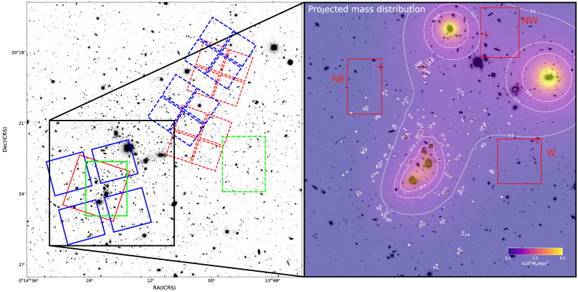
Figure 6: Left: Magellan R-band imaging of A2744 with the JWST footprints from the GLASS-JWST-ERS program, as also shown in Figure 1 from Treu et al. (2022). In red and blue we show the footprints of the NIRISS and NIRSpec pointings, respectively, while in green we plot the HFF central pointing of the cluster and parallel field (dashed). Dashed lines correspond to parallel NIRCam pointings. Right: Total projected mass distribution obtained from the best-fit LM-model, in units of $\rm 10^{9}\leavevmode\nobreak\ M_{\odot}\leavevmode\nobreak\ kpc^{-2}$, overlaid on the HST/F814W image. The red rectangles indicate the assumed priors for the positions of the three WL clumps from Medezinski et al. (2016), while the red crosses show the obtained best-fit positions.

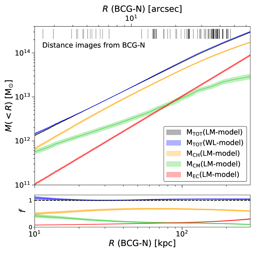
Figure 7: Top: Cumulative total mass distribution of A2744 as a function of the projected distance $R$ from the northern BCG obtained from the reference lens model. The different components of the total mass are shown: cluster halo (CH), cluster members (CM, including the BCG), and external clump (EC). The distances of the observed multiple images from the BCG-N are plotted using small vertical bars. Bottom: Ratio between the projected mass profiles obtained for the different color-coded mass components and the total cluster mass.

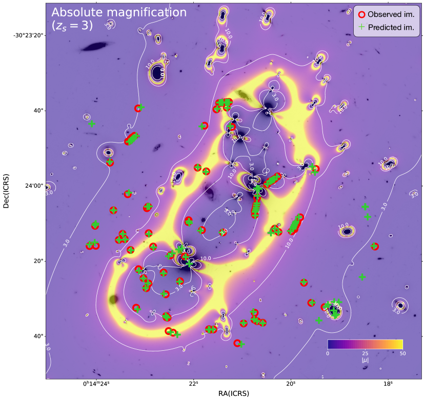
Figure 8: Absolute magnification map computed at $z_{\rm s}=3$. The red circles indicated the observed positions of the 90 multiple images, while the green crosses show the predicted positions obtained with our best-fit LM-model.

The combination of Hubble Space Telescope (HST) high-resolution imaging with mainly ground-based spectroscopic follow-up of lens galaxy clusters has enabled a broad range of science cases, from the charaterization of the dark matter distribution in cluster cores (Grillo et al., 2015; Limousin et al., 2016; Cerny et al., 2018; Diego et al., 2020) to cluster physics (Bonamigo et al., 2017, 2018; Annunziatella et al., 2017; Montes, 2022), from cluster galaxy evolution (Annunziatella et al., 2016; Mercurio et al., 2021) and the study of high-redshift galaxies (Coe et al., 2013; Vanzella et al., 2021; Meštrić et al., 2022) to cosmological analyses (Jullo et al., 2010; Caminha et al., 2016; Grillo et al., 2018). This has motivated numerous imaging programs with HST, such as the Cluster Lensing and Supernova survey with Hubble (CLASH, Postman et al., 2012), the Hubble Frontier Fields program (HFF, Lotz et al., 2017), the REionization LensIng Cluster Survey (RELICS, Coe et al., 2019) and the Beyond Ultra-deep Frontier Fields And Legacy Observations (BUFFALO, Steinhardt et al., 2020) surveys. In parallel, follow-up spectroscopic campaigns have allowed to build high-precision and accurate strong lensing mass models (e.g., Grillo et al., 2016; Caminha et al., 2019; Lagattuta et al., 2019; Bergamini et al., 2021b), impacting directly the precision and accuracy of subsequent cluster lensing applications (Meneghetti et al., 2020; Grillo et al., 2018; Vanzella et al., 2021; Meneghetti et al., 2022). The advent of the James Webb Space Telescope (JWST) will push to new frontiers the studies mentioned above. In this context, the GLASS James Webb Space Telescope Early Release Science program (hereafter GLASS-JWST-ERS; JWST-ERS-1324: PI Treu, Treu et al., 2022) has recently obtained the deepest ERS data, by pointing at the galaxy cluster Abell 2744.

Abell 2744 (A2744 hereafter, see Figure 1), at a redshift of $z=0.3072$, is a massive, X-ray luminous, merging galaxy cluster (Allen, 1998; Ebeling et al., 2010) that has been the target of extensive multi-wavelength observations. The detection of a central radio halo, and a large radio-relic in the North-East region of the cluster, led to the classification of A2744 as a recent merging system (Giovannini et al., 1999; Govoni et al., 2001). Subsequent XMM-Newton and Chandra X-ray observations, combined with rich optical spectroscopy, revealed numerous substructures in the cluster field (Kempner & David, 2004; Braglia et al., 2009; Owers et al., 2011; Eckert et al., 2015). In addition, studies on the spatial distribution and kinematics of member galaxies suggest a complex internal structure in A2744 (see for instance Couch & Sharples, 1987; Girardi & Mezzetti, 2001; Braglia et al., 2009), showing a bimodal velocity distribution of member galaxies, with a high velocity component (Owers et al., 2011). Following the detection of the first strong lensing (SL) features in the core of the cluster (Smail et al., 1997), A2744 has also been the subject of numerous lensing analyses, from SL free-form (Lam et al., 2014; Wang et al., 2015) and parametric (Johnson et al., 2014; Jauzac et al., 2015; Mahler et al., 2018; Richard et al., 2021, hereafter R21), weak-lensing (WL, Medezinski et al., 2016), to joint SL+WL models (Merten et al., 2011; Jauzac et al., 2016). Due to its lensing strength, A2744 was included as one of the six galaxy clusters in the HFF program with HST (Lotz et al., 2017), collecting some of the deepest high-resolution imaging of a cluster field. While the HFF observations led to the identification of a very large number of photometric multiple images (up to $\sim 180$, see Jauzac et al., 2015), the sample of secure systems remained fairly small, which has been shown to potentially introduce biases in total mass reconstructions (Grillo et al., 2015; Johnson et al., 2017). In particular, thanks to spectroscopic follow-up observations within the Grism Lens-Amplified Survey from Space survey (GLASS, Treu et al., 2015a; Schmidt et al., 2014), Wang et al. (2015) provided spectroscopic redshift measurements for 8 background sources. The avenue of MUSE (Multi Unit Spectroscopic Explorer, Bacon et al., 2012) follow-up observations of A2744, combined with deep HFF imaging, enabled the number of spectroscopically confirmed multiple images to significantly rise (Mahler et al., 2018; Richard et al., 2021), leading to more accurate cluster mass models.

In this work, we further exploit archival high-resolution HST imaging and MUSE spectroscopy to build an improved strong lensing model of A2744. The new model includes the largest set of spectroscopically confirmed multiple images obtained so far in this cluster field and internal kinematics of cluster galaxies to independently constrain the subhalo total mass component. The new sample of multiple images consists of multiply lensed clumps within resolved extended sources. These additional systems are especially efficient at constraining tightly the position of the critical lines locally (see for instance Grillo et al., 2016; Bergamini et al., 2021b).

The paper is organized as follows: Section 2 describes the HST imaging and spectroscopic data-sets used to develop the new lens model of A2744. In Section 3, we detail the adopted methodology for the strong lens modeling, together with the selection of the multiple images and cluster members. Our results and strong lensing online tool are presented in Sections 4 and 5, respectively, and our main conclusions are drawn in Section 6.

Throughout this work, we adopt a flat $\Lambda$CDM cosmology with $\Omega_{m}=0.3$ and $H_{0}=70\,\mathrm{km\,s^{-1}\,Mpc^{-1}}$. Using this cosmology, a projected distance of $1\arcsec$ corresponds to a physical scale of 4.528 kpc at the A2744 redshift of $z=0.3072$. All magnitudes are given in the AB system.

2 Data

This section presents the photometric and spectroscopic data sets used in this work.

2.1 HST imaging

As part of the Hubble Frontier Fields program (HFF, Proposal ID: 13495, Lotz et al., 2017), A2744 is one of the cluster fields with the deepest high-resolution observations obtained with HST. The cluster was imaged, from October 2013 to July 2014, in the optical and near-infrared with seven different bands from the Advanced Camera for Surveys (ACS; F435W, F606W, F814W) and the Wide Field Camera 3 (WFC3; F105W, F110W, F140W, F160W). The Frontier Fields observations, including ancillary data from previous HST programs with the same filters, were reduced with the HST science data products pipeline (Koekemoer et al., 2014). The HFF obervations of A2744 were recently extended out to a larger radius, thanks to the BUFFALO survey (Steinhardt et al., 2020) that has provided shallower imaging of the outskirts of the six HFF clusters. In the following analysis, we focus on the core of the galaxy cluster and defer for future work an extended strong lensing analysis. We thus exploit the Frontier Fields HST mosaics with a pixel scale value of $0\arcsec.03$.

2.2 VLT/MUSE & ancillary spectroscopy

A2744 has also been the target of extensive spectroscopic campaigns with several instruments. In particular, we use archival observations from the MUSE integral field spectrograph, mounted on the VLT (Very Large Telescope, Bacon et al., 2012), obtained within the GTO Program 094.A-0115 (PI: Richard). The data, consisting of four MUSE pointings, are described in Mahler et al. (2018) (see Figure 1 for the exposure time within each MUSE pointing), while the reduction process is presented in R21. The MUSE data cube is reduced and analyzed following the procedure adopted in Caminha et al. (2017a, b, 2019), using the standard reduction pipeline (version 2.8.5, Weilbacher et al., 2020). In addition, we use the auto-calibration method and the Zurich Atmosphere Purge (ZAP, Soto et al., 2016) to improve the data reduction. The data have a FWHM value of $0\arcsec.61$. We proceed to remeasure the redshifts of objects classified as either cluster members or multiple images in R21. The 1-dimensional spectra of these objects are extracted within a $0.\arcsec 8$ radius circular aperture, while we apply custom apertures for faint sources, based on their estimated morphology from the HST imaging. We exploit spectral templates, as well as the identification of emission lines to build our redshift catalogs. The reliability of each redshift measurement is then quantified with the following Quality Flag (QF) assignments: insecure (QF = 1), likely (QF = 2), secure (QF = 3), and based on a single emission line (QF = 9).

In addition, A2744 was targeted for 4.4h with the wide-field multi-object spectrograph VIMOS (VIsible Multi-Object Spectrograph) betweeen August 14-16, 2004 as part of the ESO Large Program 169.A-0595 (PI: Böhringer). The spectroscopic catalog, presented in Braglia et al. (2009), includes 395 non-stellar objects with a spectroscopic confirmation. The cluster was again observed using the AAOmega multi-object spectrograph on the 3.9m Anglo-Australian Telescope (AAT) between 12–18 September 2006. Combined with previous (in particular the VIMOS catalog), Owers et al. (2011) provided spectroscopic redshifts measurements for 1237 non-stellar objects within $\sim 15\arcmin$ of the cluster center, of which 343 were identified as cluster members. Finally, the GLASS (Grism Lens Amplified Survey from Space) HST WFC3/IR grism GO program (Treu et al., 2015a; Schmidt et al., 2014) provided reliable redshift measurements for 81 non-stellar objects, with a quality flag of probable or secure.

3 Strong lensing modeling

We develop a new lens model of A2744 using the publicly available software LensTool (Kneib et al., 1996; Jullo et al., 2007; Jullo & Kneib, 2009), which reconstructs the total mass distribution of a galaxy cluster by exploiting a Bayesian technique. This code was very successful at reconstructing the mass distribution of several galaxy clusters and was among the best performing codes in the Frontier Fields Lens Modeling Comparison Project (Meneghetti et al., 2017). The best-fit parameters are found by minimizing a $\chi^{2}$ function, which quantifies the goodness of the lens model in reproducing the point-like positions of the observed multiple images. This statistics is defined as:

$$\chi^{2}(\boldsymbol{\xi}):=\sum_{j=1}^{N_{fam}}\sum_{i=1}^{N_{im}^{j}}\left(\frac{\left\|\mathbf{x}_{i,j}^{obs}-\mathbf{x}_{i,j}^{pred}(\boldsymbol{\xi})\right\|}{\Delta x_{i,j}}\right)^{2},$$ (1)

where $\mathbf{x}_{i,j}^{obs}$ represents the observed position of the $i^{th}$ multiple image of the $j^{th}$ background source (images from the same source are called a family of multiple images), and $\mathbf{x}_{i,j}^{pred}$, its predicted position, given the set of model free parameters $\boldsymbol{\xi}$. $\Delta x_{i,j}$ is the error associated to the position of the image.

While the best-fit model corresponds to the set of values of model free parameters for which the $\chi^{2}(\boldsymbol{\xi})$ assumes its minimum value, we quote in the following the values for the parameters, and their associated errors, from the $50^{th}$, $16^{th}$, and $84^{th}$ percentiles of the marginalized posterior distributions. Before sampling the posterior distributions, the initial positional uncertainty for each image, $\Delta x_{i,j}$, is re-scaled so that the $\chi^{2}$ value is close to the number of degrees of freedom in the model, defined as: $\mathrm{dof}=2\times[N^{tot}_{im}-N_{fam}]-N_{freepar}$.

Moreover, we also consider and quote the root-mean-square separation between the observed and model-predicted positions of the multiple images as another figure of merit to quantify the goodness of a lens model, which is estimated as:

$$\Delta_{rms}=\sqrt{\frac{1}{N_{im}^{tot}}\sum_{i=1}^{N_{im}^{tot}}\left\|\boldsymbol{\Delta}_{i}\right\|^{2}},$$ (2)

where $\boldsymbol{\Delta}_{i}=\boldsymbol{x}_{i}^{obs}-\boldsymbol{x}_{i}^{pred}$ is the separation between the observed and predicted positions of the $i$-th image.

In this section, we present the catalog of multiple images used in the model optimization, the selection and stellar kinematic measurements of member galaxies, and a summary of the adopted mass parametrization (see e.g., Bergamini et al., 2019, for a detailed description).

3.1 Multiple images

In this work, we consider previous identifications of multiple image systems presented in R21 and reanalyze the HST multi-band imaging and the MUSE data-cube (see Section 2). The selection of secure samples of multiple images is crucial when building accurate and high-precision cluster mass models, to avoid potential biases introduced by less reliable constraints (Grillo et al., 2015; Johnson et al., 2017). Therefore, we construct our sample by considering only secure systems, that are spectroscopically confirmed by our VLT/MUSE analysis with a QF value $\geq 2$. In addition, we introduce a Positional Quality Flag (QP) that is then translated into different values for the initial positional uncertainty, $\Delta x_{i,j}$ in Equation 1, assumed in the lens model (see Figure 1). Each image is given a value of QP=1 (compact HST emission), QP=2 (diffuse or elongated HST emission) or QP=3 (MUSE only detection).

As illustrated in Figure 2 (bottom), the final sample of multiple image systems included in the lens model spans a large redshift range, between $z=1.69$ and $z=5.73$, with a total of 90 multiple images from 30 background sources (see Table 2). This represents the largest spectroscopic sample of multiple images adopted so far for A2744. The multiple image positions are shown in Figure 1 and their properties are summarized in Table 3. The observed image positions are used as constraints in the lens model, providing in total 180 observables and 60 free parameters for the positions of the corresponding sources. All systems included in our lens model are discussed and compared below to the Gold sample of R21. The resulting cumulative distribution of the distances of the multiple images included in the lens models is shown in Figure 3, and compared to that from R21.

Systems 1, 2, 3, 4, and 26 appear as extended images, clearly showing several resolved emission regions. In in this work, we use as constraints all the multiply lensed clumps that can be securely identified. From these systems we build a total number of 118 observational constraints, compared to the 46 from R21. This significant increase in the number of constraints in the innermost region of the cluster is illustrated in Figure 3. An example of the new identifications is highlighted in the zoom-in insets in Figure 1 for systems 1, 2 and 3.

All images within Systems 6, 8, 18, 22, 34, 42, 62, 63 and 64 are included both in the catalog from R21 and ours, with no discrepancies in the redshift values.

Systems 5, 105, 47 and 147, that form several extended images in the northernmost region of the cluster’s core, are not included in our image sample. While we measure a redshift value in agreement with that from R21, no clear counter image positions can be identified from the HST imaging.

Systems 10, 24, 30, 31, 41 and 61 have all a secure (QF=2 or QF=3) spectroscopic confirmation for only one of the multiple images. The remaining images have either a tentative (QF=1) or no redshift measurement. Therefore these systems cannot be considered in the secure sample.

System 33 is composed of three multiple images. Images 33.1a and 33.1b are in common in the two catalogs (with no redshit discrepancy) while image 33.1c is not considered in ours as no redshift measurement is possible.

System 37 has a redshift measurement for one of the two images included in R21. This measurement was obtained with the Low Resolution Imager and Spectrograph (LRIS) at the Keck-I telescope (Mahler et al., 2018). As the redshift cannot not be confirmed with MUSE, we do not include this system in our sample.

Finally, no redshift measurement was possible for Systems 39 and 40. Thus, we remove them from our secure catalog.

3.2 Cluster members selection & stellar kinematics

Cluster member galaxies are selected based both on spectroscopic (see Section 2.2) and multi-band HST photometric (see Section 2.1) information.

Spectroscopically confirmed cluster members are identified as those galaxies, brighter than $m_{\rm F160W}=24$, and with rest-frame ($z=0.3072$) relative velocities within $3000\leavevmode\nobreak\ \rm km\,s^{-1}$, which corresponds to the redshift range [0.28-0.34]. We mainly exploit the MUSE data-cube to identify 162 galaxies with a reliable redshift estimate (i.e. with a QF $\geq$ 2). We also include member galaxies based on spectrocpic measurements from ancillary data sets with publicly available catalogs: 32 galaxies are securely identified from the AAT/AAOmega observations (Owers et al., 2011), 5 objects from GLASS (Treu et al., 2015a; Schmidt et al., 2014), 2 from the VIMOS survey (Braglia et al., 2009), and 1 galaxy from Couch & Sharples (1987). 28 spectroscopic galaxies from the ancillary AAT/AAOmega catalogue fall outside of the HST/WFC3 field of view. We therefore adopt the following color-magnitude relation to infer the F160W magnitudes: $m_{F814}-m_{F160}=2.51-0.0797\times m_{F814}$.

We complete the spectroscopic sample by selecting 23 additional photometric, bright ($m_{\rm F160W}\leq 24$,) members based on a convolution neural network (CNN) technique, which identifies cluster members using multi-band HST image cutouts together with an extensive spectroscopic coverage, as part of the CLASH-VLT program combined with MUSE archival observations (see Angora et al., 2020, for a detailed description of the method). The training set is composed of $\sim$3300 samples, in 14 CLASH and HFF clusters (with a redshift between $z=0.2-0.6$). When tested on the spectroscopic sample of A2744, we measure a completeness level of 88% and a high degree of purity, equal to 95%.

In summary, our final high-purity cluster member catalog, which is integrated in the following lensing analysis, consists of 225 member galaxies in total, covering an area of $\sim 14\rm\leavevmode\nobreak\ arcmin^{2}$. Within this sample, 202 (or $\sim 90\%$) are spectroscopically confirmed, and 23 are photometric members. We show in Figure 2 the distribution of these cluster galaxies as a function of their magnitude in the HST/F160W band, and their properties are listed in Table 4.

As presented in Bergamini et al. (2019, 2021b), we further exploit the MUSE data-cube to measure the line-of-sight stellar velocity dispersion for a large sub-set of cluster members. We extract the spectra for the 162 cluster galaxies securely confirmed by the MUSE data within $0.8^{\prime\prime}$ radius apertures (comparable to the MUSE PSF). Velocity dispersions are then measured using the publicly available software Penalized Pixel-Fitting method (Ppxf, Cappellari & Emsellem, 2004; Cappellari, 2017), over the wavelength range [3700-5700] Å. In order to exploit reliable measurements in the subsequent lensing analysis, we limit the sample to galaxies with $\langle S/N\rangle>10$ and $\sigma_{0}>50\leavevmode\nobreak\ \mathrm{km\leavevmode\nobreak\ s^{-1}}$ (see e.g., Bergamini et al., 2019, 2021b). In addition, we perform a visual inspection of the imaging and the fitted spectra, resulting in the exclusion of three faint galaxies whose spectra are contaminated by the light from BCG-S and BCG-N. The final sample of cluster members with internal kinematics includes thus 85 galaxies, down to $m_{\rm F160W}\sim 22$ (see Figure 2, top). The resulting measured $\sigma_{0}$ values are presented in Figure 4, as a function of their HST/F160W magnitude values.

3.3 Total mass parametrization

		Input parameter values and assumed priors
		$x\,\mathrm{[arcsec]}$	$y\,\mathrm{[arcsec]}$	$e$	$\theta\ [^{\circ}]$	$\sigma_{LT}\,\mathrm{[km\ s^{-1}]}$	$r_{core}\,\mathrm{[arcsec]}$	$r_{cut}\,\mathrm{[arcsec]}$
Cluster-scale halos	$1^{st}$ Cluster Halo	$-5.0\,\div\,5.0$	$-5.0\,\div\,5.0$	$0.0\,\div\,0.9$	$0.0\,\div\,180.0$	$300.0\,\div\,1500.0$	$0.0\,\div\,30.0$	$2000.0$
	$2^{nd}$ Cluster Halo	$-27.9\,\div\,-7.9$	$-30.1\,\div\,-10.1$	$0.0\,\div\,0.9$	$0.0\,\div\,90.0$	$300.0\,\div\,1500.0$	$0.0\,\div\,30.0$	$2000.0$
	$1^{st}$ Ext. clump	$99.5$	$86.0$	$0.0$	$0.0$	$100.0\,\div\,1500.0$	$0.001$	$2000.0$
	$2^{nd}$ Ext. clump	$138.3$	$99.9$	$0.0$	$0.0$	$100.0\,\div\,1500.0$	$0.001$	$2000.0$
	$3^{rd}$ Ext. clump	$24.2$	$155.8$	$0.0$	$0.0$	$100.0\,\div\,1500.0$	$0.001$	$2000.0$
Subhalos	BCG-N	$0.0$	$0.0$	$0.0\,\div\,0.9$	$0.0\,\div\,180.0$	$200.0\,\div\,400.0$	$0.0001$	$0.1\,\div\,50.0$
	BCG-S	$-17.9$	$-20.0$	$0.0\,\div\,0.9$	$0.0\,\div\,180.0$	$200.0\,\div\,400.0$	$0.0001$	$0.1\,\div\,50.0$
	Scaling relations	$\boldsymbol{N_{gal}=}223$	$\boldsymbol{m_{\mathrm{F160W}}^{ref}=}17.34$	$\boldsymbol{\alpha=}0.40$	$\boldsymbol{\sigma_{LT}^{ref}=}190.0\,\div\,300.0$	$\boldsymbol{\beta_{cut}=}0.41$	$\boldsymbol{r_{cut}^{ref}=}0.5\,\div\,10.0$	$\boldsymbol{\gamma=}0.20$

		Optimized output parameters
		$x\,\mathrm{[arcsec]}$	$y\,\mathrm{[arcsec]}$	$e$	$\theta\ [^{\circ}]$	$\sigma_{LT}\,\mathrm{[km\ s^{-1}]}$	$r_{core}\,\mathrm{[arcsec]}$	$r_{cut}\,\mathrm{[arcsec]}$
Cluster-scale halos	$1^{st}$ Cluster Halo	$-1.5^{+0.3}_{-0.4}$	$-0.1^{+0.8}_{-0.9}$	$0.6^{+0.1}_{-0.1}$	$90.3^{+2.5}_{-2.7}$	$522.7^{+32.1}_{-32.2}$	$6.8^{+0.8}_{-0.7}$	$2000.0$
	$2^{nd}$ Cluster Halo	$-18.2^{+0.5}_{-0.5}$	$-15.7^{+0.4}_{-0.4}$	$0.4^{+0.1}_{-0.1}$	$53.3^{+2.6}_{-2.8}$	$633.9^{+21.1}_{-22.3}$	$7.6^{+0.6}_{-0.6}$	$2000.0$
	$1^{st}$ Ext. clump	$99.5$	$86.0$	$0.0$	$0.0$	$201.3^{+124.0}_{-73.8}$	$0.001$	$2000.0$
	$2^{nd}$ Ext. clump	$138.3$	$99.9$	$0.0$	$0.0$	$933.4^{+32.3}_{-47.4}$	$0.001$	$2000.0$
	$3^{rd}$ Ext. clump	$24.2$	$155.8$	$0.0$	$0.0$	$775.8^{+29.6}_{-30.8}$	$0.001$	$2000.0$
Subhalos	BCG-N	$0.0$	$0.0$	$0.3^{+0.2}_{-0.2}$	$129.6^{+20.9}_{-25.4}$	$221.8^{+13.0}_{-12.0}$	$0.0001$	$36.9^{+8.7}_{-10.5}$
	BCG-S	$-17.9$	$-20.0$	$0.8^{+0.1}_{-0.1}$	$26.1^{+3.7}_{-3.0}$	$304.4^{+9.4}_{-10.7}$	$0.0001$	$34.9^{+9.5}_{-9.6}$
	Scaling relations	$\boldsymbol{N_{gal}=}223$	$\boldsymbol{m_{\mathrm{F160W}}^{ref}=}17.34$	$\boldsymbol{\alpha=}0.40$	$\boldsymbol{\sigma_{LT}^{ref}=}235.7^{+21.8}_{-19.0}$	$\boldsymbol{\beta_{cut}=}0.41$	$\boldsymbol{r_{cut}^{ref}=}5.8^{+2.5}_{-1.8}$	$\boldsymbol{\gamma=}0.20$

Table 1: Top: Input parameters of the reference model (LM-model) for the galaxy cluster A2744 presented in this work. A single number is quoted for fixed parameters. When a flat prior on a free parameter is considered, the boundaries of the prior separated by the $\div$ symbol are reported. The number of galaxies optimized trough the scaling relations ($N_{gal}$), and the reference magnitude ($\boldsymbol{m_{\mathrm{F160W}}^{ref}}$) are also reported. Bottom: Optimized values of the output parameters of the reference lens model. For each free parameter, we quote the median and the 16-th, and 84-th percentiles of the posterior distribution.

Comparison between published lens models
Model	$N_{\mathrm{images}}$	$N_{\mathrm{sources}}$	$\Delta_{rms}\,\mathrm{[\arcsec]}$
This work	90	30	0.37
R21	83	29	0.67

Table 2: Comparison between our new lens model for A2744 and other published models for the same cluster. $N_{\mathrm{images}}$ is the number of multiple image used as model constraints, $N_{\mathrm{sources}}$ is the number of background sources, and $\Delta_{rms}\,\mathrm{[\arcsec]}$ is the total root-mean-square displacement between observed and predicted image positions (see Eq. 2).

LensTool adopts a parametric approach, where the total mass distribution of a galaxy cluster is decomposed into the sum of several components. Extended HST imaging from the BUFFALO survey reveals several massive secondary structures in the outskirts, residing at distances between $\sim 600-775$ kpc from the BCG-N, and forming multiply imaged systems in the vicinity. The massive structures, confirmed to be at the cluster’s redshift based on ancillary spectroscopy (see Section 2.2), can introduce a non-negligible perturbation in the positions of the multiple images in the core, and therefore impact the derived mass distribution (e.g., Acebron et al., 2017). In this work, we explore two different mass parametrizations of A2744. In the reference model, labeled LM-model, we model the cluster’s environment as inferred from the extended BUFFALO imaging, while in the WL-model, we implement the results from previous WL studies (Medezinski et al., 2016). The total mass distribution of the cluster is thus decomposed into the following mass contributions:

$$\phi_{tot}=\sum_{i=1}^{N_{h}}\phi_{i}^{halo}+\sum_{j=1}^{N_{bcg}}\phi_{j}^{BCG}+\sum_{k=1}^{N_{g}}\phi_{k}^{gal}+\sum_{l=1}^{N_{s}}\phi_{l}^{ENV}.$$ (3)

The first component refers to the profiles used to parameterize the cluster-scale halos of the cluster (mainly made of dark matter). The second term corresponds to the mass contribution of the two brightest cluster galaxies (BCGs), BCG-N and BCG-S in Figure 1, which are individually optimized in the lens model. The third sum describes the mass contribution of the cluster member galaxies (the subhalo component) to the total cluster mass, modeled within scaling relations. Finally, the fourth and last component models the contribution from structures in the cluster environment (where the parametrization of the two mass models differ). A detailed description of the modeling of each component is provided below.

Both the cluster and subhalo mass component ($\phi_{i}^{halo}$, $\phi_{j}^{BCG}$ and $\phi_{k}^{gal}$) are described using dual pseudo-isothermal elliptical mass distributions (dPIEs, Limousin et al., 2005; Elíasdóttir et al., 2007; Bergamini et al., 2019). This profile is characterized by seven free parameters: the position (x, y); the ellipticity (defined as $e=\frac{a^{2}-b^{2}}{a^{2}+b^{2}}$, where a and b are the semi-major and semi-minor axes of the ellipsoid, respectively); the position angle $\theta$ computed counterclockwise from the west direction; the central velocity dispersion $\sigma_{0}$ ;the core radius $r_{core}$; and the truncation radius $r_{cut}$. We note that, instead of using $\sigma_{0}$, LensTool adopts a scaled version of this quantity, identified as $\sigma_{LT}$, such that $\sigma_{LT}=\sigma_{0}\sqrt{2/3}$.

The cluster-scale component of our new lens models ($\phi_{i}^{halo}$) is parametrized by two not truncated elliptical dPIEs, which are centered on the BCGs, denominated BCG-N and BCG-S in Figure 1. The halos are left free to move within a small range around the BCG positions (see Table  1).

Due to the presence of radial arcs in the vicinity of both BCGs (namely systems 2 and 4, see Figure 1 and Table 3), and to improve their reconstruction, the parameters describing the mass contribution, and the ellipticity, of both BCGs are individually optimized (i.e., they are modeled outside of the scaling relations). This consists of 4 additional free parameters for each profile.

Cluster member galaxies ($\phi_{j}^{gal}$) are described using singular circular dPIEs whose velocity dispersions, $\sigma^{gal}_{LT,i}$, and truncation radii, $r^{gal}_{cut,i}$, scale with the galaxy luminosity, $L_{i}$, according to the following scaling relations (which are used to sensibly reduce the number of free parameters of the lens model):

$$\sigma^{gal}_{LT,i}=\sigma^{ref}_{LT}\left(\frac{L_{i}}{L_{ref}}\right)^{\alpha},\quad r^{gal}_{cut,i}=r^{ref}_{cut}\left(\frac{L_{i}}{L_{ref}}\right)^{\beta_{cut}}.$$ (4)

The reference luminosity $L_{ref}=17.34$ corresponds to the BCG-N (see Figure 1) magnitude in the HST F160W band. Following Bergamini et al. (2021b), we fix $\alpha=0.40$ and $\beta_{cut}=0.41$. As described in Bergamini et al. (2019), these values are inferred from the measured inner stellar kinematics of 85 cluster member galaxies obtained by exploiting the MUSE data (see Section 3.2). A large, uniform, prior is assumed for $r^{ref}_{cut}$.

As previously mentioned, the effect of the cluster environment is implemented in different ways in our SL modeling. In our reference model, LM-model, we include the mass contribution from the 3 brightest galaxies in the northern region of the cluster (called also external clumps), which are modeled as singular isothermal sphere profiles (SIS). Their positions are fixed to that of the light (see Table 1), while their velocity dispersion values are optimized within flat large priors that account for the galaxy and large-scale DM distribution (adding 3 free parameters in total). LM-model has a total number of 25 free parameters related to the mass parametrization. For the WL-model, the effect of the cluster environment is modeled based on the results from the WL analysis presented in Medezinski et al. (2016), using deep imaging from Subaru/Suprime-Cam. Besides the main structure associated with the cluster’s core, three additional sub-structures were detected with a high significance value of $\gtrsim 5\sigma$. These sub-structures (labeled W, NE and NW in Medezinski et al., 2016, and in Figure 6), are modeled as SIS profiles. We adopt the best-fit positions and mass parameters from Medezinski et al. (2016) (Table 4), and their statistical uncertainties through large flat priors, in our lens model. Each halo adds thus 3 free parameters, the position, ($x$, $y$) and the velocity dispersion, $\sigma_{0}$. The WL-model has a total number of 31 free parameters related to the mass parametrization.

The priors assumed for the parameters of the mass profiles included in our reference lens model, LM-model, are summarized in the upper part of Table  1, while the optimized values are reported in the bottom.

4 Results

The final $\Delta_{rms}$ value of our new reference lens model (LM-model) is $0.37\arcsec$, corresponding to an improvement of approximately a factor of $\sim 2$ compared to the previous value ($0.67\arcsec$) obtained by R21, where a smaller sample of multiple images was used to constrain the lens model. In Figure 5, we show the separations, along the $x$ and $y$ directions, between the observed and model predicted positions of the 90 multiple images (see also the red and green symbols in Figure 8). The figure shows that the model can reproduce accurately the observed position of the images in those cluster regions where the spatial density of image constraints is higher (more than five multiple images within $5\arcsec$). This result demonstrates that a large sample of secure multiple images, including resolved substructures within extended images (e.g., see the cutouts in Figure 1), and distributed all around the cluster field, is an important ingredient to develop high-precision cluster strong lensing models (see also Grillo et al., 2016; Bergamini et al., 2021a, Bergamini et al. in prep.).

On the other hand, the optimization of the WL-model, which includes the three WL halos, leads to a $\Delta_{rms}$ value of $0.44\arcsec$, therefore significantly larger than our reference model. This underscores the better ability of the light-traces-mass approach in reproducing the mass distribution of the external region of the cluster.

Figure 9: The graphical interface of our new Strong Lensing Online Tool (SLOT) allows for a full and easy access to high-level products, including the statistical uncertainties, of our lens models. The link will be available upon publication.

In Figure 6, we show the resulting total projected mass distribution of A2744 from our reference best-fit lens model superimposed to the HST/F814W image. We note that our lens model can be considered accurate up to $50$-$60\arcsec$ from the BCG-N (this is the largest distance at which secure multiple images have been identified). Model predictions outside that region are extrapolations and can, therefore, be prone to systematic errors.

Figure 7 shows that the total projected cluster mass distribution within 300 kpc from the BCG-N (in black), and its different components (as described in Equation 3). Due to the degeneracies between model parameters, a clear separation between the mass contributions from the BCGs and the cluster halo is not possible. The contribution of the member galaxies to the cluster total mass decreases as a function of the distance from the cluster center. At radii larger than 100 kpc, the mass contribution of the external clumps dominates over that of the subhalo. At a radius of 200 kpc, the total mass of the cluster is $M_{\rm tot}=(1.77\leavevmode\nobreak\ \pm 0.07)\times 10^{14}\,\mathrm{M_{\odot}}$, including both the statistical and systematic uncertainties (see Figure 7).

In Fig.  4, we show the $\sigma$-luminosity relation. For a proper comparison of the lensing velocity dispersion of the galaxies with the observed ones, the values are corrected for the spectroscopic aperture (0.8″), as detailed in (see Bergamini et al., 2019)). The cluster member scaling relations inferred from the lens models are in excellent agreement with the kinematic results, although no prior on the $\sigma_{LT}^{ref}$ value is assumed. We have checked that by imposing a prior on that value, we find no significant difference in the $\Delta_{rms}$ value (i.e., $\sim 0.03\arcsec$ higher).

In Figure 8, we show the absolute magnification map computed for a background source at $z=3$. While the magnification values are significantly different from one at large distances from the cluster center, we caution that these values are extrapolations in regions that lack strong lensing constraints. Relatively large magnification values are also supported by the presence of several strong lensing features that are visible at distances between $\sim 600-775$ kpc from the BCG-N, revealed in the BUFFALO imaging. The formation of these distant gravitational arcs is attributed to the presence of secondary cluster clumps surrounding A2744. Their mass is expected to be comparable to those of the main cluster (see Table  1).

5 SLOT: Strong Lensing Online Tool

The A2744 lens model presented in this work will be made publicly available with the publication of this paper. In order to allow interested users to access and exploit the model results, we have developed a graphical interface, pictured in Figure 9. The new Strong Lensing Online Tool (SLOT) will allow astronomers to take full advantage of the predictive and statistical results of our high-precision strong lensing model for their research, both for studies on cluster lenses and high-redshift sources. For example, SLOT can be used to: compute magnification values, with a careful estimation of the associated statistical errors, for all the sources in the field of A2744; obtain the predicted positions of the counter-images of every source defined by the user; derive and download maps of projected cluster total mass, deflection angle, magnification, etc. A description of the functionality of SLOT and the user manual can be found in the SLOT webpage (the link will be available upon publication).

6 Conclusions

We have presented a new high-precision strong lensing model for the galaxy cluster A2744. A careful inspection of the HST and MUSE data has allowed us to create a secure image data-set counting 90 multiple images (from 30 background sources) whose point-like positions are used to constrain the lens model. This is currently the largest multiple image catalog compiled for this cluster. Our lens model also includes the information coming from the measured stellar kinematics of 85 member galaxies that is used to accurately characterize the subhalo component of the cluster. This component counts a total of 225 galaxies (including the two cluster BCGs), 202 of which are spectroscopically confirmed cluster members. The gravitational lens A2744 is strongly affected by the presence of massive structures in the North-West region of the cluster, at distances between $\sim 600-775$ kpc from the BCG-N. The contribution of these outer massive structures is taken into account by using three additional SIS profiles in our reference lens model fixed on the positions of the three brightest galaxies in that area.

The final $\Delta_{rms}$ value of our reference model, LM-model, is equal to $0.37\arcsec$ representing a significant step forward with respect to previous SL models for the same cluster, and with the same data-set (e.g., R21). The inclusion of the sub-structures within several extended sources as model constraints, including the radial arcs, has allowed us to accurately characterize the inner total mass distribution of the cluster and the position of the cluster critical lines.

In addition, we have found that accounting for the mass distribution of the cluster outside the core, particularly using the light of three prominent cluster galaxies as total mass tracers, is a key ingredient to an accurate prediction of the positions of the multiple images.

Finally, we have presented a new publicly available graphical interface, called Strong Lensing Online Tool (SLOT). Interested users, even non-lensing experts, can exploit the predictive power and the full statistical information of the lens model presented in this work through a user-friendly graphical interface.

We plan to apply our new high-precision strong lensing model for the first analysis of the GLASS-JWST-ERS observations, specifically to make use of magnification values and uncertainties for high-$z$ lensed sources. Clearly, JWST imaging and spectroscopic data will reveal a much larger number of multiply imaged sources with resolved substructures, over a more extended redshift range, which we will employ to improve the lens model presented in this work.

Appendix A Multiple images

We present the catalog of the 90 secure multiple images (from 30 background sources), that are included as constraints in our SL model, and that represent the largest secure sample in the A2744 cluster field. All systems are discussed, and compared to the catalog presented in R21, in Section 3.1.

Table 3: Catalog of the spectroscopic multiple images included in the SL modeling of A2744.

ID	R.A.	Decl	$\rm z_{spec}$	QF	QP
	deg	deg
1.1a	3.597561	-30.403925	1.688100	3	1
1.1b	3.595963	-30.406808	1.688100	2	1
1.1c	3.586226	-30.409986	1.688100	3	1
1.2a	3.597072	-30.404723	1.688100	3	1
1.2b	3.596395	-30.406143	1.688100	3	1
1.2c	3.585748	-30.410100	1.688100	3	1
1.3a	3.597756	-30.403530	1.688100	3	2
1.3b	3.595528	-30.407199	1.688100	3	2
1.3c	3.586459	-30.409871	1.688100	3	2
1.4a	3.598082	-30.403980	1.688100	1	1
1.4b	3.595722	-30.407546	1.688100	1	1
1.4c	3.587383	-30.410152	1.688100	1	1
2.1a	3.583265	-30.403339	1.886800	3	1
2.1b	3.597289	-30.396712	1.886800	3	1
2.1c	3.585369	-30.399878	1.886800	3	1
2.1d	3.586412	-30.402127	1.886800	3	1
2.2a	3.583029	-30.403189	1.886800	3	1
2.2b	3.597138	-30.396639	1.886800	3	1
2.2c	3.585134	-30.399668	1.886800	3	1
2.2d	3.586438	-30.401870	1.886800	3	1
2.3a	3.582994	-30.403050	1.886800	3	1
2.3b	3.597095	-30.396580	1.886800	3	1
2.3c	3.585017	-30.399625	1.886800	3	1
2.3d	3.586394	-30.401765	1.886800	3	1
2.4a	3.582918	-30.402930	1.886800	3	1
2.4b	3.597052	-30.396527	1.886800	3	1
2.4c	3.584915	-30.399580	1.886800	3	1
2.4d	3.586353	-30.401632	1.886800	3	1
2.5a	3.582828	-30.402793	1.886800	3	2
2.5b	3.596990	-30.396469	1.886800	3	2
2.5c	3.584819	-30.399517	1.886800	3	2
2.5d	3.586322	-30.401490	1.886800	3	1
2.6a	3.582772	-30.402683	1.886800	3	2
2.6b	3.596942	-30.396421	1.886800	3	2
2.6c	3.584722	-30.399463	1.886800	3	2
2.6d	3.584719	-30.399462	1.886800	3	2
2.7a	3.582530	-30.402313	1.886800	3	2
2.7b	3.596734	-30.396291	1.886800	3	2
2.7c	3.584473	-30.399289	1.886800	3	2
2.7d	3.586236	-30.400869	1.886800	3	2
3.1a	3.588807	-30.393797	3.980500	3	1
3.1b	3.589375	-30.393857	3.980500	3	1
3.2a	3.589222	-30.393844	3.980500	3	1
3.2b	3.588965	-30.393815	3.980500	3	1
3.3a	3.589487	-30.393869	3.980500	3	1

ID	R.A.	Decl	$\rm z_{spec}$	QF	QP
	deg	deg
3.3b	3.588639	-30.393785	3.980500	3	1
4.1a	3.592126	-30.402660	3.577000	3	1
4.1b	3.595674	-30.401633	3.577000	3	1
4.1c	3.580452	-30.408946	3.577000	3	2
4.1e	3.593651	-30.405117	3.577000	3	3
4.2a	3.592098	-30.402527	3.577000	3	1
4.2b	3.595567	-30.401518	3.577000	3	1
6.1a	3.598541	-30.401792	2.017100	3	1
6.1b	3.594058	-30.407999	2.017100	3	1
6.1c	3.586433	-30.409363	2.017100	3	1
8.1a	3.589712	-30.394335	3.976400	2	2
8.1b	3.588831	-30.394202	3.976800	2	2
18.1a	3.576124	-30.404472	5.662400	3	1
18.1b	3.588377	-30.395630	5.662400	3	1
18.1c	3.590730	-30.395543	5.662400	3	1
22.1a	3.587924	-30.411608	5.284400	3	2
22.1b	3.600048	-30.404415	5.284400	3	2
22.1c	3.596592	-30.408989	5.283700	3	2
26.1a	3.593898	-30.409724	3.054200	3	1
26.1b	3.590353	-30.410575	3.054200	3	1
26.1c	3.600112	-30.402939	3.054200	9	2
26.2a	3.593993	-30.409699	3.054200	3	1
26.2b	3.590272	-30.410610	3.054200	3	1
26.3a	3.594031	-30.409604	3.054200	2	3
26.3b	3.589969	-30.410593	3.054200	2	3
33.1a	3.584712	-30.403146	5.725600	3	1
33.1b	3.584397	-30.403393	5.725600	3	1
34.1a	3.593428	-30.410834	3.784000	2	1
34.1b	3.593812	-30.410714	3.784000	3	1
34.1c	3.600711	-30.404593	3.787300	2	1
42.1a	3.597313	-30.400605	3.691900	3	1
42.1b	3.590956	-30.403252	3.691900	3	1
42.1c	3.581590	-30.408631	3.691900	3	1
42.1d	3.594245	-30.406388	3.691900	3	1
42.1e	3.592415	-30.405197	3.691900	1	3
61.1a	3.595522	-30.403485	2.950900	1	1
61.1b	3.595138	-30.404471	2.950900	3	1
62.1a	3.591326	-30.398643	4.193600	3	3
62.1b	3.590582	-30.398918	4.193600	3	3
63.1a	3.582214	-30.407142	5.661500	3	1
63.1b	3.592836	-30.407032	5.661500	3	2
63.1c	3.589153	-30.403427	5.661500	3	1
63.1d	3.598830	-30.398273	5.661500	3	1
64.1a	3.581203	-30.398734	3.408600	3	1
64.1c	3.596420	-30.394264	3.408600	3	1

Appendix B Cluster members

We present the catalog of the 225 cluster member galaxies that are included in our SL model, 202 of which are spectroscopically selected (based on the MUSE and ancillary spectroscopy, presented in Section 2.2) and 23 are identified based on HST multi-band photometry through a CNN technique (see Section 3.2).

Table 4: Catalog of the spectroscopic (top) and photometric (bottom) cluster members included in the SL modeling of A2744.

ID	R.A.	Decl	$m_{F160W}$	$\rm z_{spec}$
	deg	deg
36034	3.592037	-30.405741	17.30	0.3185
37824	3.586257	-30.400172	17.34	0.2997
835	3.589290	-30.369074	16.88	0.3002
40689	3.594796	-30.391654	17.58	0.3006
736	3.575038	-30.428344	17.69	0.3170
938	3.610666	-30.395618	17.70	0.3033
814	3.587469	-30.371246	17.76	0.3038
947	3.612408	-30.409245	17.84	0.3031
34423	3.579662	-30.409189	17.84	0.3027
40059	3.585386	-30.394279	17.89	0.3202
783	3.583084	-30.433553	18.00	0.2927
20227	3.609542	-30.382110	18.03	0.3200
39382	3.587646	-30.396426	18.07	0.3031
36210	3.592510	-30.404611	18.24	0.3150
809	3.586500	-30.367380	18.29	0.3007
697	3.566354	-30.388260	18.40	0.3025
36527	3.578511	-30.403375	18.41	0.3155
38067	3.574900	-30.398381	18.46	0.3175
740	3.575081	-30.377074	18.49	0.3142
730	3.573503	-30.422861	18.50	0.3188
37947	3.592998	-30.399330	18.57	0.3092
834	3.589103	-30.419803	18.59	0.3044
894	3.602057	-30.377689	18.60	0.3011
41259	3.593289	-30.384378	18.60	0.2964
40592	3.589220	-30.389839	18.64	0.3151
41644	3.570173	-30.386449	18.66	0.2969
37954	3.586559	-30.399391	18.70	0.3229
35061	3.573945	-30.408829	18.71	0.3135
39428	3.588152	-30.395075	18.71	0.3002
41950	3.589184	-30.387396	18.72	0.3169
38907	3.585204	-30.394649	18.81	0.3009
642	3.556336	-30.387018	18.88	0.3115
38117	3.582159	-30.398571	18.89	0.2986
39072	3.598969	-30.397533	18.90	0.3162
41856	3.585314	-30.387545	18.91	0.3008
804	3.585629	-30.366902	18.98	0.2998
37344	3.604341	-30.400124	18.98	0.3190
41440	3.605429	-30.384843	18.99	0.3112
38010	3.588385	-30.398355	19.01	0.3173
678	3.562510	-30.402406	19.05	0.3025
38930	3.588680	-30.396077	19.07	0.3020
40243	3.580953	-30.390808	19.15	0.2931
32284	3.602650	-30.416956	19.16	0.3132

ID	R.A.	Decl	$m_{F160W}$	$\rm z_{spec}$
	deg	deg
690	3.565544	-30.387093	19.16	0.2991
40478	3.571507	-30.390436	19.18	0.2965
20018	3.581566	-30.376517	19.22	0.3130
902	3.604284	-30.414554	19.25	0.3061
966	3.618050	-30.403670	19.26	0.3115
42443	3.594708	-30.389115	19.26	0.3035
40314	3.590342	-30.390939	19.26	0.2972
720	3.571365	-30.422840	19.29	0.3030
41363	3.588146	-30.385006	19.30	0.2977
692	3.565347	-30.382948	19.38	0.3030
768	3.580711	-30.418875	19.39	0.2934
956	3.615142	-30.383729	19.41	0.3061
38729	3.578864	-30.397111	19.42	0.3190
973	3.618739	-30.392932	19.42	0.3015
36892	3.587938	-30.400852	19.44	0.3150
863	3.593561	-30.426049	19.46	0.2968
35339	3.595907	-30.406213	19.49	0.3161
950	3.613184	-30.389698	19.49	0.3026
20132	3.595399	-30.380404	19.50	0.3200
921	3.607012	-30.403478	19.51	0.2966
655	3.559037	-30.410659	19.51	0.2984
32547	3.601355	-30.415365	19.51	0.3197
37068	3.605266	-30.400808	19.52	0.3197
888	3.600962	-30.417843	19.59	0.3042
41418	3.592547	-30.385314	19.62	0.3164
931	3.609576	-30.378771	19.62	0.3009
39503	3.581389	-30.393932	19.63	0.2998
634	3.555379	-30.384632	19.66	0.3007
34556	3.591721	-30.407807	19.71	0.3194
816	3.587541	-30.373945	19.71	0.2963
961	3.616679	-30.402709	19.72	0.2943
41303	3.583714	-30.384680	19.75	0.3029
33910	3.589134	-30.409573	19.75	0.3173
42149	3.598764	-30.388018	19.76	0.3027
33540	3.588817	-30.410722	19.77	0.3223
787	3.583285	-30.432301	19.78	0.2942
39646	3.578948	-30.394119	19.80	0.3191
40884	3.590278	-30.382698	19.86	0.3019
37229	3.594463	-30.400350	19.89	0.3036
33328	3.569589	-30.412164	19.95	0.2990
40270	3.594239	-30.390462	19.97	0.3163
42269	3.595506	-30.388688	19.97	0.3032
13996	3.573450	-30.377932	20.00	0.3184
39710	3.584986	-30.392877	20.01	0.2954
35693	3.587039	-30.404948	20.04	0.2987
40551	3.589520	-30.389499	20.08	0.2939
21367	3.597859	-30.405556	20.12	0.3208
40832	3.588038	-30.382557	20.17	0.3116
39876	3.580373	-30.392204	20.21	0.2935
33699	3.582507	-30.409986	20.24	0.3188
38275	3.585521	-30.397156	20.24	0.3124
41655	3.573735	-30.385976	20.26	0.2965
41651	3.573383	-30.386313	20.34	0.3079
37230	3.583991	-30.399260	20.34	0.3200
40802	3.570861	-30.382004	20.37	0.3066
36220	3.605275	-30.402932	20.39	0.3161
39283	3.600830	-30.394896	20.39	0.3061
713	3.569303	-30.384236	20.42	0.2961
20089	3.597633	-30.379200	20.51	0.2800
32768	3.585709	-30.413971	20.59	0.3023

ID	R.A.	Decl	$m_{F160W}$	$\rm z_{spec}$
	deg	deg
42195	3.578348	-30.387100	20.61	0.3076
13311	3.560070	-30.389342	20.61	0.2999
33870	3.595124	-30.409366	20.63	0.3199
35908	3.585035	-30.403315	20.63	0.3037
37609	3.578591	-30.399109	20.68	0.3054
36043	3.584377	-30.402887	20.83	0.3159
41908	3.604401	-30.384960	20.84	0.2962
34439	3.590280	-30.407401	20.92	0.3182
40032	3.593885	-30.390837	20.96	0.2970
36339	3.588145	-30.401980	20.97	0.2986
32088	3.603422	-30.416769	20.99	0.3179
38143	3.602200	-30.396988	21.01	0.3031
44545	3.578469	-30.381318	21.04	0.3179
36953	3.572810	-30.400534	21.05	0.3143
37825	3.602715	-30.397571	21.08	0.2990
40428	3.578347	-30.389464	21.12	0.2947
20064	3.577544	-30.378870	21.26	0.3080
36298	3.594832	-30.402130	21.30	0.3162
35576	3.587971	-30.404253	21.31	0.2998
40239	3.593166	-30.390349	21.33	0.3013
36849	3.596757	-30.400513	21.33	0.3167
34538	3.573400	-30.407461	21.46	0.3141
36843	3.579074	-30.400089	21.50	0.3056
40703	3.596256	-30.388517	21.54	0.2964
33671	3.583831	-30.409506	21.56	0.3023
33410	3.589721	-30.410222	21.57	0.3154
40708	3.571061	-30.388157	21.61	0.3032
38252	3.592874	-30.396356	21.61	0.2975
37214	3.585389	-30.399007	21.67	0.3006
36163	3.588499	-30.402102	21.70	0.2992
39727	3.584373	-30.391755	21.75	0.3200
41636	3.573693	-30.385685	21.79	0.2971
37542	3.584458	-30.398342	22.02	0.3235
38175	3.583312	-30.396542	22.05	0.3073
35190	3.601244	-30.404885	22.11	0.3049
38267	3.597298	-30.396046	22.15	0.3189
33803	3.593740	-30.409224	22.18	0.3033
37367	3.601857	-30.398661	22.22	0.3144
42079	3.593478	-30.387595	22.24	0.2962
8024000	3.567362	-30.400881	22.30	0.3023
34705	3.594676	-30.405899	22.31	0.3072
41265	3.578737	-30.384233	22.33	0.3168
37199	3.603831	-30.399122	22.37	0.3026
41937	3.573015	-30.387260	22.43	0.3219
35514	3.574778	-30.403672	22.43	0.3039
32680	3.592097	-30.413109	22.45	0.3067
36814	3.593414	-30.400024	22.49	0.3040
36982	3.582898	-30.399701	22.49	0.2914
40944	3.593025	-30.382970	22.50	0.3005
37231	3.581618	-30.399105	22.51	0.3049
10440000	3.569048	-30.394963	22.56	0.3077
33503	3.597475	-30.409964	22.56	0.3051
10657000	3.569981	-30.394634	22.61	0.3011
41388	3.598749	-30.384458	22.61	0.3089
36872	3.595752	-30.399971	22.62	0.3160
34828	3.592717	-30.406107	22.65	0.3187
38459	3.572068	-30.395969	22.66	0.2990
39956	3.584993	-30.390870	22.67	0.3161
33933	3.585939	-30.408434	22.71	0.3080
41467	3.586832	-30.384627	22.74	0.3085
41842	3.591221	-30.386717	22.76	0.3132

ID	R.A.	Decl	$m_{F160W}$	$\rm z_{spec}$
	deg	deg
38253	3.584471	-30.396056	22.78	0.3224
41531	3.589828	-30.385639	22.85	0.3174
4206000	3.600810	-30.409530	22.87	0.3068
36346	3.588851	-30.401771	22.89	0.3059
41930	3.608089	-30.387068	22.90	0.2962
33753	3.567161	-30.408755	22.92	0.3170
33911	3.577555	-30.408196	22.94	0.3068
39609	3.605171	-30.392616	22.98	0.3217
35436	3.589433	-30.404231	23.10	0.3184
4136000	3.590889	-30.410893	23.11	0.2983
41419	3.577521	-30.384813	23.12	0.3219
3476000	3.585092	-30.412314	23.13	0.3071
32671	3.588878	-30.413346	23.14	0.3047
35134	3.598182	-30.404825	23.15	0.3002
38748	3.579869	-30.394391	23.15	0.3201
12269000	3.577314	-30.390297	23.21	0.3131
12325000	3.605930	-30.390167	23.24	0.3059
38900	3.579626	-30.394091	23.26	0.3193
42040	3.573600	-30.387182	23.27	0.2825
10930000	3.572670	-30.393633	23.28	0.3198
35978	3.596444	-30.403275	23.28	0.2989
11577000	3.590109	-30.391576	23.31	0.3080
36776	3.584729	-30.399826	23.33	0.3002
3547000	3.566721	-30.411992	23.36	0.3002
33468	3.595517	-30.409682	23.42	0.3219
12191000	3.581882	-30.390474	23.44	0.3229
37304	3.583931	-30.398595	23.45	0.2986
40432	3.584083	-30.388909	23.46	0.2890
34433	3.588518	-30.406316	23.47	0.3174
5079000	3.586480	-30.407004	23.54	0.3199
3795000	3.592497	-30.412103	23.55	0.3089
10265000	3.597219	-30.395534	23.56	0.3196
12018000	3.605043	-30.391671	23.64	0.2986
8216000	3.597727	-30.400602	23.69	0.3155
4938000	3.582862	-30.408838	23.70	0.3007
35340	3.588510	-30.404209	23.73	0.3198
7420000	3.568412	-30.402023	23.80	0.3054
8330000	3.569485	-30.399955	23.83	0.3049
14319	3.598659	-30.383098	23.38	–
15369	3.575794	-30.380405	23.72	–
9490	3.574867	-30.397183	23.80	–
10127	3.566005	-30.393924	21.12	–
12163	3.607988	-30.390726	23.14	–
14786	3.593635	-30.382101	23.16	–
5889	3.578093	-30.405740	23.76	–
15699	3.594368	-30.378664	22.52	–
15508	3.578849	-30.379423	23.88	–
7737	3.597161	-30.402246	23.97	–
13676	3.568877	-30.385314	20.36	–
15624	3.575140	-30.378524	21.58	–
5421	3.606797	-30.405592	20.39	–
14659	3.601322	-30.382501	23.43	–
2937	3.580614	-30.414102	22.85	–
15691	3.571676	-30.379704	23.55	–
9592	3.607186	-30.397230	23.56	–
2818	3.576712	-30.414622	23.56	–
16198	3.573701	-30.376807	22.99	–
5315	3.581605	-30.407436	23.58	–
3313	3.575661	-30.413496	23.61	–
15308	3.570284	-30.380798	23.64	–
14680	3.570831	-30.382935	23.67	–