Dimensional Transmutation from Non-Hermiticity

Abstract

Dimensionality plays a fundamental role in the classification of novel phases and their responses. In generic lattices of 2D and beyond, however, we found that non-Hermitian couplings do not merely distort the Brillouin zone (BZ), but can in fact alter its effective dimensionality. This is due to the fundamental non-commutativity of multi-dimensional non-Hermitian pumping, which obstructs the usual formation of a generalized complex BZ. As such, basis states are forced to assume “entangled” profiles that are orthogonal in a lower dimensional effective BZ, completely divorced from any vestige of lattice Bloch states unlike conventional skin states. Characterizing this reduced dimensionality is an emergent winding number intimately related to the homotopy of non-contractible spectral paths. We illustrate this dimensional transmutation through a 2D model whose topological zero modes are protected by a 1D, not 2D, topological invariant. Our findings can be readily demonstrated via the bulk properties of non-reciprocally coupled platforms such as circuit arrays, and provokes us to rethink about the fundamental role of geometric obstruction in the dimensional classification of topological states.

Introduction.– Dimensionality is fundamental in determining possible physical phenomena, such as in Anderson localization Lee and Fisher (1981); Azbel (1982); Lherbier et al. (2008) and critical phase transitions Aharony et al. (1976); Alekhin (2005). In particular, symmetry-protected topological phases can be systematically classified based on Bott periodicity in the number of dimensions, via the tenfold-way Altland and Zirnbauer (1997); Schnyder et al. (2008); Ryu et al. (2010); Kitaev (2009); Stone et al. (2010); Morimoto and Furusaki (2013); Chiu et al. (2013). More recently, this classification is greatly enriched Gong et al. (2018); Liu et al. (2019); Li et al. (2019a); Kawabata et al. (2019); Zhou and Lee (2019); Li and Mong (2021) in non-Hermitian lattices, which are increasingly studied theoretically Bergholtz et al. (2021); Hu and Hughes (2011); Esaki et al. (2011); Lee and Chan (2014); Lee et al. (2014); Leykam et al. (2017); Hu et al. (2017); Lieu (2018); Yin et al. (2018); Jiang et al. (2018); Li et al. (2018); Shen et al. (2018); Borgnia et al. (2020); Pan et al. (2020); Yao et al. (2018); Budich et al. (2019); Lee (2021); Shen and Lee (2021); Kawabata and Ryu (2021); Lee (2022); Qin et al. (2023a) and in photonic, mechanical, electrical and cold-atom experiments Gao et al. (2015); Zeuner et al. (2015); Xu et al. (2016); Xiao et al. (2017); Feng et al. (2017); Weimann et al. (2017); Parto et al. (2018); Weidemann et al. (2020); Helbig et al. (2020); Hofmann et al. (2020); Xiao et al. (2020); Ghatak et al. (2020); Zou et al. (2021); Stegmaier et al. (2021); Wang et al. (2021); Gao et al. (2021); Zhang et al. (2021); Shang et al. (2022); Weidemann et al. (2022); Li et al. (2022); Zhang et al. (2022a); Rosa-Medina et al. (2022); Zhang et al. (2023a).

Usually, it is taken for granted that the dimensionality of the topological invariant Thouless et al. (1982); Kohmoto (1985); Qi et al. (2008); Schindler et al. (2018); Lee et al. (2018a, 2019); Luo and Zhang (2019); Tuloup et al. (2020); Jiang and Lee (2022) coincides with that of the physical space. This is because they are defined in reciprocal (momentum) space, which should be of the same dimension as the physical lattice, at least in Euclidean space. Even among enigmatic non-Hermitian phenomena featured latelyZhang et al. (2022b); Lin et al. (2023); Yao and Wang (2018); Xiong (2018); Lee and Thomale (2019); Song et al. (2019a, b); Longhi (2019); Zhang et al. (2020); Yokomizo and Murakami (2019); Yang et al. (2020); Lee and Longhi (2020); Longhi (2020); Claes and Hughes (2021a); Okuma et al. (2020); Schindler and Prem (2021); Li et al. (2021a); Okuma and Sato (2021); Li et al. (2021b); Guo et al. (2021); Li and Lee (2022); Yang et al. (2022); Rafi-Ul-Islam et al. (2022a); Xue et al. (2022); Zhang et al. (2022c); Rafi-Ul-Islam et al. (2022b); Tai and Lee (2022); Longhi (2021); Kawabata et al. (2020); Longhi (2022); Gu et al. (2022); Okugawa et al. (2020); Claes and Hughes (2021b); Qin et al. (2023b); Lei et al. (2023); Guo et al. (2023), the highly distorted effective Brillouin zone (BZ) is still indexed by states living in the same dimensionality.

Yet we discover, surprisingly, that in 2D and beyond, non-Hermiticity can in fact change the effective BZ dimensionality. This holds true for generic non-Hermitian lattices beyond the simplest monoclinic structures, whenever the lattice is bounded (as all realistic lattices should be). Hence, the effective band structure of a $D$-dim lattice may in reality live in $D^{\prime}$$<$$D$ dimensions, and be classified by $D^{\prime}$ instead of $D$-dim topology.

Underlying this dimensional transmutation is a hitherto unnoticed geometric obstruction, specifically the non-commutativity in the equilibration of states that have been directionally amplified i.e. “pumped” by the non-Hermitian skin effect (NHSE) along different directions. This “equilibration process” is the mathematical elimination of non-reciprocity upon switching to the generalized Brillouin zone, conventionally constructed one dimension at a time. Fundamentally resulting from emergent non-locality Yao and Wang (2018); Lee et al. (2020a), it is reminiscent of the non-commutativity of magnetic translations from the non-locality of flux threading, as epitomized by the Aharonov-Bohm effect Berry (1984); Bachtold et al. (1999); Gou et al. (2020).

Non-Hermitian equilibration and its non-commutativity.–  Consider a generic lattice Hamiltonian under open boundary conditions (OBCs)

$$H=\sum_{\bm{x};\alpha,\beta}\sum_{\{\bf e\}}h_{\mathbb{e}}^{\alpha\beta}c^{\dagger}_{\bm{x}+\mathbb{e},\alpha}c_{\bm{x},\beta},$$ (1)

where $\mathbb{e}$ ranges over all coupling displacements from each unit cell, and $\alpha,\beta$ are sublattice components. When the couplings have asymmetric amplitudes $|h_{\mathbb{e}}^{\alpha\beta}|\neq|h_{-\mathbb{e}}^{\beta\alpha}|$, all left/right moving states are invariably attenuated/amplified by a factor of $|h_{\mathbb{e}}^{\alpha\beta}|/|h_{-\mathbb{e}}^{\beta\alpha}|$ per unit cell shifted Hatano and Nelson (1996, 1997); Longhi et al. (2015). This leads to a dramatic density accumulation of directionally NHSE amplified states at lattice boundaries or impurities. When it is just simple exponential build-up, they are NHSE eigenstates; in more esoteric critical cases, they can assume special scale-free eigenstate profiles Li et al. (2020); Kawabata et al. (2020); Liu et al. (2020a); Yokomizo and Murakami (2021); Li et al. (2021a); Kawabata et al. (2022); Qin et al. (2023b). In generic higher-dimensional lattices that we focus on, such boundary accumulations have not been properly understood.

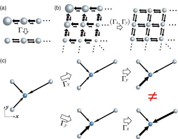
Figure 1: Failure of effective BZ construction in 2D through conventional basis rescaling. a) To obtain the effective BZ of a nearest-neighbor 1D lattice, all couplings can simply be “symmetrized” through a change of basis known as the equilibration operation $\Gamma$. b) Higher-dimensional “unentangled” lattices can still be similarly symmetrized via independent equilibrations $\Gamma_{x},\Gamma_{y},...$ c) Generic “entangled” lattices of 2D and beyond cannot be completely equilibrated, since equilibrations $\Gamma_{j}$ do not commute in general; shown is a minimal example where $\Gamma_{x}\Gamma_{y}\neq\Gamma_{y}\Gamma_{x}$(non-commutativity), i.e. where symmetrization in one direction can un-symmetrize the coupling components in the other direction (arrow thickness depict coupling strength). Hence obtaining the effective BZ through naive NHSE-inspired equilibration (change-of-basis to the generalized BZ) is doomed to failure.

Since the Bloch eigenstates that define the original BZ are highly distorted by non-Hermitian pumping (directed amplification), all “bulk” properties such as band topology, transport and geometry will be radically modified. To correctly characterize them, it is necessary to construct the effective BZ where the spatially non-uniform pumped eigenstates are “equilibrated” to approximately resemble Bloch states. This equilibration is mathematically a transformation to a basis where the NHSE is eliminated - in that basis, the couplings appear symmetrized and the NHSE no longer acts Yang et al. (2020); Lee et al. (2020a). The simplest illustrative example, well-known in the NHSE literature, is the 1D “Hatano-Nelson” chain with asymmetric nearest-neighbor couplings $h_{\pm\hat{x}}=he^{\mp\kappa}$ (Fig. 1a) Hatano and Nelson (1996, 1997); Longhi et al. (2015); Claes and Hughes (2021a). Under OBCs, its eigenstates assume the boundary-localized form $\psi_{\text{HN}}(x)\sim e^{-\kappa x}$[Fig. 1a (balls increasing in size)], which can be “equilibrated” into the bulk through a basis rescaling operator $\Gamma$: $c^{\dagger}_{x}\rightarrow e^{\kappa x}c^{\dagger}_{x}$, $c_{x}\rightarrow e^{-\kappa x}c_{x}$. (We write $\Gamma_{j}$ for $\Gamma$ corresponding to a boundary in the $j$-th direction). At the same time, $\Gamma$ also “balances” the equilibrated couplings, as shown in Fig. 1a, as well as induce an effective complex deformed BZ viz. $c^{\dagger}_{k}=\sum_{x}e^{ikx}c^{\dagger}_{x}\rightarrow\sum_{x}e^{i(k-i\kappa)x}c^{\dagger}_{x}=\sum_{x}z(k)^{x}c^{\dagger}_{x}$ where $-i\log z(k)=k-i\kappa$ is the complexified momentum. The assumption here is that, even though translation invariance is lost due to OBCs, the eigenmodes are still approximately labeled by appropriately discretized wavenumbers, albeit with an additional $e^{-\kappa x}$ spatial factor to account for NHSE accumulation.

In higher-dimensions $D$, only the simplest lattices i.e. monoclinic lattice for $D=2$ (Fig. 1b) can be “unentangled” into separate sets of 1D chains $H(k_{1},k_{2},...)=H^{1}_{\text{1D}}(k_{1})\oplus H^{2}_{\text{1D}}(k_{2})\oplus...$ . For these, the equilibration operator $\Gamma_{j}$ can be analogously applied whenever OBCs are taken along the $j$-th direction.

But generically, most $D\geq 2$ lattices are “entangled” due to non-trivial inter-chain couplings, and this NHSE-inspired equilibration procedure (generalized BZ construction) fails to give the correct equilibrated lattice couplings and hence effective BZ. Consider the minimal model with three non-orthogonal asymmetric hoppings from each site non-trivially “entangling” the two lattice directions (Fig. 1c). Let’s derive the boundary-accumulated eigenstates when its lattice (not explicitly shown) is under OBCs in both $x$ and $y$ directions. At each equilibration step $\Gamma_{j}$, the combined coupling strength component in the $j$-th direction are to be “balanced”: in Fig. 1c, the $\Gamma_{x}$ operation modifies the original couplings negligibly because the x-components are already approximately equal, but not so for $\Gamma_{y}$. But therein lies the paradox: exchanging the order of performing the equilibrations $\Gamma_{x},\Gamma_{y}$ yield different equilibrated couplings, even though the effective lattice should of course not depend on the order in which the $x$,$y$-OBCs are taken. This non-commutativity of $\Gamma_{x}$ and $\Gamma_{y}$, even for such a minimal example, suggests that physical states are pumped in a peculiar non-local manner, and an entirely new approach is needed for correctly characterizing the effective BZ whenever a multi-dimensional lattice cannot be trivially decoupled into 1D chains, as further explained in the Appendix.

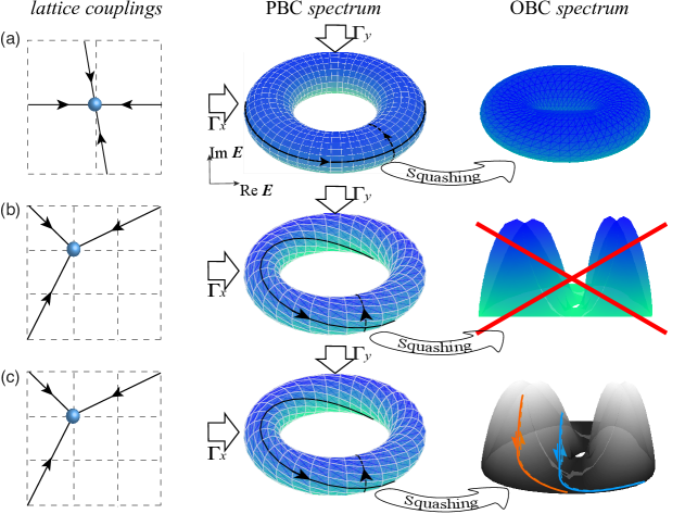
Figure 2: Non-commutativity of NHSE equilibration violates the requirement of vanishing OBC spectral winding. a) An “unentangled” lattice admits fully commuting equilibration operators $\Gamma_{x},\Gamma_{y}$ that completely “squashes” (flattens) its PBC spectral torus $E_{\text{2D}}$ into a “flattened” OBC torus $\bar{E}_{\text{2D}}$, reminiscent of 1D cases, where the OBC spectrum consists of PBC spectral loops “squashed” into interior curves Yang et al. (2020). b) An “entangled” lattice is subject to non-commuting equilibrations $\Gamma_{x}\Gamma_{y}\Gamma_{x}^{-1}\Gamma_{y}^{-1}\neq\mathbb{I}$, such that its PBC spectrum can no longer be completely “squashed” into a valid OBC spectrum with no spectral winding, akin to a filled balloon. c) The correct OBC spectrum of the “entangled” 2D lattice is traced out by up to two 1D homotopy paths (blue, orange) on the incompletely squashed spectral torus that avoid any spectral winding. The tori so illustrated do not live in 3D, but are projections on the 2D energy plane, being composed of collections of 1D spectral loops.

Dimensional transmutation from non-commutative equilibration.– We next show how multi-dimensional non-Hermitian directed NHSE amplification i.e. pumping on the energy spectrum advocates an effective BZ of a different, lower dimension. Consider a 2D model $H_{\text{2D}}(k_{x},k_{y})$ in momentum space. Under periodic boundary conditions (PBCs), its spectrum $E_{\text{2D}}(k_{x},k_{y})$ generically resembles a deformed torus projected onto a 2D plane (Fig. 2), since it takes complex values and is parametrized by two periodic momenta. Going from PBCs to OBCs, this spectrum $E_{\text{2D}}\rightsquigarrow\bar{E}_{\text{2D}}$ must necessarily be “squashed” i.e. flattened into lines or curves in the complex plane by non-Hermitian pumping, since under OBCs, any 1D subsystem i.e. any 1D loop traced by $E_{\text{2D}}(k_{x},k_{y})$ with fixed $k_{x}$ or $k_{y}$ must enclose zero area (be degenerate) in the complex energy plane: $\oint\partial_{k_{j}}\log(\bar{E}_{\text{2D}}(\bm{k})-E_{0})\,\text{d}k_{j}=0$ for all $E_{0}\in\mathbb{C}$, $j=x,y$ Zhang et al. (2020). Intuitively, this is because nontrivial spectral winding requires non-reciprocity, but OBC eigenstates are fully “equilibrated” at the boundaries and are no longer pumped non-reciprocally .

However, the spectral squashing in 2D is often not straightforward like in 1D, where equilibration always amounts to a complex BZ deformation $e^{ik}\rightarrow z(k)\rightarrow e^{i(k-i\kappa(k))}$ that completely squashes $E_{\text{1D}}(k)\rightarrow E_{\text{1D}}(k)(k-i\kappa(k))=\bar{E}_{\text{1D}}(k)$ into a degenerate spectral loop with no spectral winding i.e. $\bar{E}_{\text{1D}}(k)=\bar{E}_{\text{1D}}(k^{\prime})$ for some $k\neq k^{\prime}$. As sketched in Fig. 2a for an “unentangled” 2D lattice, the Hamiltonian can be written by $H({\bm{k}})=\sum_{n}A_{n}(k_{x})\exp(ink_{y})$ with the solution $z_{y}$ of $\sum_{n}A_{n}(k_{x})z_{y}^{n}\sin(q_{y})=0$ independent of $k_{x}$, $\Gamma_{x}$ and $\Gamma_{y}$ is allowed to successively “squash” the spectral torus until it contains no non-degenerate loops enclosing nonzero area, since the lattice trivially decouples into two non-parallel 1D chains. However, for an “entangled” 2D lattice (Fig. 2b,c), $|A_{n}(k_{x})/A_{-n}(k_{x})|$ dependent of $k_{x}$, $\Gamma_{x}\Gamma_{y}\Gamma_{x}^{-1}\Gamma_{y}^{-1}\neq\mathbb{I}$ and the “squashing” cannot be complete - picture a filled balloon which can be compressed in one direction, but not squashed in all directions simultaneously. As the incompletely “squashed” spectral torus still contains non-degenerate loops, the only solution is to exclude them from the effective BZ itself. In this case, the effective BZ can only be spanned by the homotopy generator independent from any non-degenerate spectral loop, and can only be of 1D despite the physical lattice being of 2D. Fig. 2c shows two possible loops (blue, orange) that enclose zero area on the complex $E$ plane, and either (or both) of them would rightly span the effective BZ. Fig. 3a shows an example where successive application of $\Gamma_{x}$ followed by $\Gamma_{y}$ gives the incorrect spectrum (dark blue), different from the numerically obtained spectrum (blue). As such, even though effective 1D BZs possess well-defined complex momenta viz. $z(k)=e^{i(k-i\kappa(k))}$ in 2D or higher, in general $z_{j}(\bm{k})\neq e^{i(k_{j}-i\kappa_{j}(\bm{k}))}$, $j=x,y,...$, defying the well-established NHSE framework.

Construction of dimensionally transmutated effective BZ.– We now construct the effective BZ of a 1-component example of the type in Fig. 2b,c::

$$H_{\text{2D}}=\sum_{\bm{x}}t_{1}c^{\dagger}_{\bm{x}}c_{\bm{x}+\alpha\hat{x}+a\hat{y}}+t_{2}c^{\dagger}_{\bm{x}}c_{\bm{x}-\beta\hat{x}+a\hat{y}}+t_{3}c^{\dagger}_{\bm{x}}c_{\bm{x}-\beta\hat{x}-b\hat{y}}.$$ (2)

Applying the ansatz $\psi_{2D}(x,y)\propto z_{x}^{x}z_{y}^{y}$ for an eigenstate, we obtain the energy relation

$$E_{\text{2D}}(z_{x},z_{y})=t_{1}z^{\alpha}_{x}z^{a}_{y}+t_{2}z^{-\beta}_{x}z^{a}_{y}+t_{3}z^{-\beta}_{x}z_{y}^{-b}.$$ (3)

Here, no assumption is made about the boundary conditions, and the assertion is that $E_{\text{2D}}(z_{x},z_{y})$ yields the correct eigenenergies given appropriate forms of $z_{x},z_{y}$.

To correctly obtain the effective BZ from $E_{\text{2D}}(z_{x},z_{y})$, we would need to treat the effects of both $x$ and $y$-OBCs on equal footing, such the order of opening up OBCs in different directions do not matter, as physically expected. This can be achieved by alternately implementing the two OBCs one at a time, by considering the other momentum as a parameter. Given a quasi-1D energy function $E_{\text{1D}}(z)$, we determine the effective BZ by finding a complex effective momentum function $-i\log z(k)$, $k\in[0,2\pi)$, such that every energy eigenvalue $E=E_{\text{1D}}(z(k))$ corresponds to at least two different $k$ solutions with identical $|z(k)|$ Lee and Thomale (2019); Yokomizo and Murakami (2019). In a trivial case without non-Hermitian pumping, we simply have $z(k)=e^{ik}$, such that the effective and original BZs coincide. For $E_{\text{1D}}(z)=Az^{p}+Bz^{-q}$ corresponding to left(right) hoppings over $p$ ($q$) sites, we have from Sect. I of sup

$$z(k)=\left(\frac{B\sin qk}{A\sin pk}\right)^{\frac{1}{p+q}}e^{e^{i\frac{2\pi\nu}{p+q}}}e^{ik}=e^{-\kappa_{\text{1D}}(k)}e^{ik}\ ,$$ (4)

for $k\in(-\pi/(p+q),\pi/(p+q)]$, $\nu=1,2,...,p+q$ labeling the solution branch. The decay function $e^{-\kappa_{\text{1D}}(k)}$ encodes how non-Hermitian directed amplification distorts the Bloch phase factor $e^{ik}$.

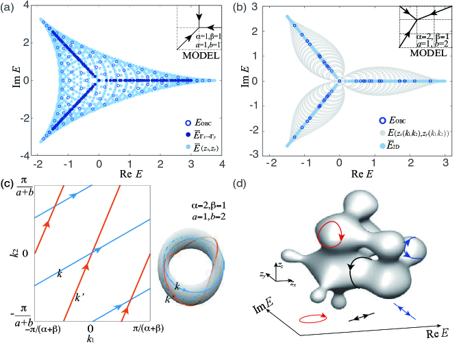
Figure 3: Dimensionally transmutated effective BZ gives the correct OBC spectrum. a) Sequentially applying $\Gamma_{x}$ and then $\Gamma_{y}$ ($x$-OBCs and then $y$-OBCs) yields an incorrect OBC spectrum $\bar{E}_{\Gamma_{x}\rightarrow\Gamma_{y}}$ (Dark blue) for the illustrative “entangled” 2D lattice $H=\sum_{\bm{x}}{\color[rgb]{0,0,0}2}c^{\dagger}_{\bm{x}+\hat{x}}c_{\bm{x}}+c^{\dagger}_{\bm{x}+\hat{y}}c_{\bm{x}}+c^{\dagger}_{\bm{x}-\hat{x}-\hat{y}}c_{\bm{x}}$ (no dimensional transmutation ), at odds with the symmetrically obtained $\bar{E}(z_{x},z_{y})$ (light blue), which reproduces the exact numerical $E_{\text{OBC}}$ (blue circles). b) Necessity of dimensional transmutation of the BZ: For our model $H_{\text{2D}}$ (Eq. 2), the effectively 1D $\bar{E}_{\text{2D}}$ (light blue) agrees with the numerical $E_{\text{OBC}}$ (blue circles), while the unconstrained $E_{\text{2D}}$ from Eqs. 3 and 5a,5b gives extraneous eigenenergies (gray). The systems of 3a and 3b belong to scenarios depicted in Figs. 2a and 2b,c respectively. c) The effective 1D BZ is given by the union of 1D winding paths (blue, red for $k,k^{\prime}$ respectively) on the $k_{1}$-$k_{2}$ 2-torus. d) $\mathscr{M}$ (gray blob) of an illustrative 3D model, with effective BZ given by its blue and black loops that correspond to degenerate spectral loops in the complex $E$ plane below.

By applying Eq. 4 on $z_{x},z_{y}$ of Eq. 3 separately, we obtain $z_{x}^{\alpha+\beta}=(t_{2}+t_{3}z_{y}^{-(a+b)})/(t_{1}\sin\alpha k_{1})\sin\beta k_{1}\,\text{e}^{i(\alpha+\beta)k_{1}}$ and $z_{y}^{-(a+b)}=(t_{2}+t_{1}z_{x}^{\alpha+\beta})/(t_{3}\sin bk_{2})\sin ak_{2}\,\text{e}^{-i(a+b)k_{2}}$, where we have used $k_{1},k_{2}$ instead of $k_{x},k_{y}$ to emphasize that they may not be conjugate momenta to the $x,y$ coordinates. We can simultaneously solve these to obtain

$$z_{x}^{\alpha+\beta}=\frac{t_{2}}{t_{1}}\frac{(\sin ak_{2}+e^{i(a+b)k_{2}}\sin bk_{2})e^{i(\alpha+\beta)k_{1}}\sin\beta k_{1}}{e^{i(a+b)k_{2}}\sin\alpha k_{1}\sin bk_{2}-e^{i(\alpha+\beta)k_{1}}\sin\beta k_{1}\sin ak_{2}},$$ (5a)

$$z_{y}^{a+b}=\frac{t_{3}}{t_{2}}\frac{e^{i(a+b)k_{2}}\sin\alpha k_{1}\sin bk_{2}-e^{i(\alpha+\beta)k_{1}}\sin\beta k_{1}\sin ak_{2}}{(\sin\alpha k_{1}+e^{i(\alpha+\beta)k_{1}}\sin\beta k_{1})\sin ak_{2}}.$$ (5b)

We reiterate a major distinction between the $z_{x},z_{y}$ above and the effective “generalized” BZ of NHSE systems: In the latter, the BZ is “generalized” in the sense that $z_{j}$, $j=x,y$ encapsulates complex momentum via $-i\log z_{j}=k_{j}-i\kappa_{j}(\bm{k})$, with $\kappa_{j}(\bm{k})$ representing the complex deformation. But in Eqs. 5a, 5b, $-i\log z_{j}$ manifestly do not correspond to any single well-defined complex momentum (recall that $\psi_{2D}(x,y)\propto z_{x}^{x}z_{y}^{y}$). Even though $k_{1},k_{2}$ are the individual “momenta” associated with quasi-1D chains within $H_{\text{2D}}$, they are now “entangled”, as evident in the highly nonlinear functional form of Eqs. 5a,5b.

Importantly, the $z_{x},z_{y}$ from Eqs. 5a and 5b still do not describe the correct effective BZ unless $k_{1},k_{2}$ are further constrained, since we have not eliminated the possibility of $E(z_{x},z_{y})$ exhibiting nontrivial windings as one of $k_{1}$ or $k_{2}$ is varied over a period (Sect. II and III of sup ). Indeed, from Fig. 3b, naive substitution of the unconstrained $z_{x},z_{y}$ into Eq. 3 gives extraneous eigenenergies across the complex plane (gray), different from the numerical OBC spectrum (blue circles) which exhibits no spectral winding.

For our model, all spectral windings vanish along the two 1D parametrization paths $(k_{1},k_{2})=(bk,\beta k)$ and $(k_{1},k_{2})=(ak^{\prime},\alpha k^{\prime})$, as rigorously shown in Sect. III of sup . Indeed, in Fig. 3b, the union of these energies $\bar{E}_{\text{2D}}(k)=E_{\text{2D}}(z_{x}(k),z_{y}(k))$ and $\bar{E}^{\prime}_{\text{2D}}(k^{\prime})=E_{\text{2D}}(z_{x}(k^{\prime}),z_{y}(k^{\prime}))$ also agree with the numerical OBC spectrum. The union of the 1D loops traced by $k$ and $k^{\prime}$ forms the dimensionally transmutated effective BZ, as illustrated in Fig. 3c and the Appendix.

Interestingly, this effectively 1D BZ reveals a new avenue of topological winding, with winding numbers $\text{GCD}(a,\alpha)$ and $\text{GCD}(b,\beta)$ describing how the sectors $k^{\prime}$ and $k$ loop around the $k_{1}$-$k_{2}$ torus. (both windings $=2$ in Fig. 3c). Physically, $k_{1},k_{2}$ represent the non-Bloch wavenumbers from separately taking OBCs in each direction; yet, when both OBCs are simultaneously applied, the effective BZ collapses into closed 1D paths that mixes $k_{1}$ and $k_{2}$. As such, these winding numbers capture the amount of “entanglement” caused by 2D non-Hermitian pumping.

Generalizations.– The construction of the dimensionally-transmutated effective BZ from our particular $H_{\text{2D}}$ lattice can be generalized to a generic model $H$ in $D$ dimensions. First, acting on the ansatz eigenstate $\psi_{D}(\bm{x})\propto\prod_{j}^{D}z_{j}^{x_{j}}$, we express the model as a multivariate polynomial $E(\bm{z})=\sum_{\mu}t_{\mu}\prod_{j}z_{j}^{l_{\mu j}}$, where $l_{\mu j}$ is the range of the $\mu$-th hopping $t_{\mu}$ in the $j$-th direction. Next, we apply the $D$ equilibrations $\Gamma_{j}$, $j=1,...,D$ separately on $E(\bm{z})$, such that each becomes a quasi-1D problem in $z_{j}$, with all the components of $\tilde{z}=(z_{1},...,z_{j-1},z_{j+1},...,z_{D})$ as spectator parameters. Solving for the effective 1D BZs for each of them sup ; Yokomizo and Murakami (2019); Lee et al. (2020a); Tai and Lee (2022) i.e. replacing each $z_{j}$ by appropriate $e^{-\kappa_{j}(\tilde{z})}e^{ik_{j}}$ (of which Eq. 4 is a special case), we obtain $D$ relations (Sect. III of sup ) $\mathscr{F}_{j}(\tilde{z};k_{j})=0$. Inverting these relations, we will in principle obtain $D$ expressions $z_{j}=\mathcal{F}_{j}(\bm{k})$ where $\bm{k}\in\mathbb{T}^{D}$, which generalize Eqs. 5a, 5b. In general, this nonlinear inversion may have to be performed numerically, and yields a highly complicated $D$-dimensional base manifold $\mathscr{M}$ in $\bm{z}$-space, possibly with cusps and singularities that give rise to higher dimensional esoteric gapped transitions Li et al. (2020).

The effective dimensional-transmutated BZ depends crucially on the topology of $\mathscr{M}$. Specifically, it is $\mathscr{M}/\{\mathcal{L}\}$, where $\{\mathcal{L}\}$ is the span of homotopy loops $l$ on $\mathscr{M}$ in which $E(\bm{z}(l))$ exhibits nontrivial spectral winding i.e. the effective BZ is union of submanifolds of $\mathbb{T}^{D}$ parametrized by $(k^{\prime}_{1},...,k^{\prime}_{d})$, $d<D$, such that the recovered OBC spectrum $\bar{E}(\bm{k}^{\prime})=E(\bm{z}(\bm{k}^{\prime}))$ exhibits trivial spectral winding in all directions, as detailed in Sect. III of sup As schematically sketched in Fig. 3d for a 3D model, the effective BZ consists of the blue and black loops which wind around $\mathscr{M}$ (gray), not the red loop which encloses nonzero spectral area.

Dimensional transmutated topology.– The fundamental dimensional modification of the effective BZ by non-Hermitian pumping (directed amplification) is not just a mathematical subtlety, but a very physical phenomenon with experimentally observable consequences. In the following, we illustrate a 2D lattice whose topological zero modes are protected by a 1D, not 2D, topological invariant due to dimensional transmutation of its BZ. We consider the 2-component 2D model

$$H_{\text{topo}}(\bm{z})=\left(\begin{array}[]{cc}0&z_{x}^{\alpha}+z_{x}^{-\beta}+z_{x}^{-\beta}z_{y}^{-a-b}+cz^{-a}_{y}\\ z_{y}^{a}&0\\ \end{array}\right)\ ,$$ (6)

with constant $c$ introduced such that the PBC spectrum $E_{\text{topo}}(e^{ik_{x}},e^{ik_{y}})=\pm\sqrt{E_{\text{2D}}(e^{ik_{x}},e^{ik_{y}})+c}$ is gapped.

When regarded as a 2D model, $H_{\text{topo}}$ is topologically trivial by construction, as can be seen from its Pauli decomposition $H_{\text{topo}}=\left[(H_{12}+iH_{21})\sigma_{x}+(H_{12}-iH_{21})\sigma_{y}\right]/2$, which contains only two Pauli matrices and is thus of trivial 2nd homotopy. However, the effective bulk description of $H_{\text{topo}}$ is actually 1D, not 2D, since $E_{\text{topo}}(z_{x},z_{y})$ and $E_{\text{2D}}(z_{x},z_{y})$ are conformally related and must therefore possess identical effective 1D BZs Lee et al. (2020a); Tai and Lee (2022). Under OBCs, an effectively 1D Hamiltonian possesses topological zero modes if the phase windings of $H_{12}(z)$ and $H_{21}(z)$ around $z=0$ are both nonzero and of opposite signs Yao and Wang (2018); Lee and Thomale (2019); if there is more than one BZ sector, the windings should be added, as performed in Sect IV of sup . This is indeed the case in Fig. 4a, with the windings of $H_{12}$ and $H^{\prime}_{12}$ summing to $-1$, and that of $H_{21}$ and $H^{\prime}_{21}$ summing to $1$. Correspondingly, these windings protect the isolated zero modes in the double OBCs spectrum (black diamond in Fig. 4b); these modes are topological since they appear in the double PBCs bandgap. Despite being protected by 1D topological winding, they do not appear in the quasi-1D scenario with only $x$-OBCs (light blue).

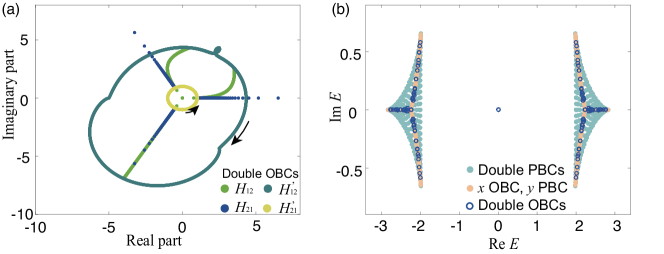
Figure 4: Dimensional transmutated topology in 2-band model  a) Despite being a 2D model, $H_{\text{topo}}$ exhibits nontrivial topological winding in its effectively 1D BZ, as seen from the zero windings of $H_{12}(k)$ and $H^{\prime}_{12}(k^{\prime})$ summing to $-1$, and that of $H_{21}(k)$ and $H^{\prime}_{21}(k^{\prime})$ summing to $1$. b) Although protected by 1D topological winding, in-gap zero modes for $H_{\text{topo}}$ appear under double OBCs (black), and not quasi-1D single OBC (light blue). Parameters are $t_{1}=t_{2}=t_{3}=1$ and $c=5$.

Discussion.– Existing higher-dimensional non-Hermitian studies i.e. Chern or higher-order skin-topological characterizations Ezawa ; Lee and Qi (2014); Yao et al. (2018); Luo and Zhang (2019); Lee et al. (2019); Kawabata et al. (2020); Groenendijk et al. (2021) have mostly been based on simple hyperlattices. Beyond that, in generic lattices with “entangled” couplings, we discover that non-Hermitian pumping does not commute, transmuting the momentum-space lattice (BZ) to an effectively lower dimension. As a fundamentally dynamical phenomenon, this dimensional transmutation contrasts with the dimensional reduction in topological classification Qi et al. (2008); Ryu et al. (2010); Tantivasadakarn (2017), as well as the emergence of an extra scaling dimension in lattice-based holography approaches Qi (2013); Gu et al. (2016); Lee (2017); Hu et al. (2020).

Physically, the dimensional transmutation can be manifested through bulk response and topological properties. Topological states protected by lower-dimensional invariants can be constructed and observed in open non-reciprocal arrays with sufficiently versatile engineered couplings, such as lossy photonic resonator arrays Botten et al. (1997); Yariv (2002); Feng et al. (2017); Bergholtz et al. (2021), electrical circuits sup ; Lee et al. (2018b); Imhof et al. (2018); Helbig et al. (2019); Hofmann et al. (2019); Kotwal et al. (2021); Zhang et al. (2019); Ni et al. (2020); Helbig et al. (2020); Lee et al. (2020b); Li et al. (2019b); Zhang and Franz (2020); Hofmann et al. (2020); Lenggenhager et al. (2021); Bergholtz et al. (2021); Liu et al. (2021); Zou et al. (2021); Stegmaier et al. (2021); Liu et al. (2020b); Hohmann et al. (2022); Zhang et al. (2022a); Wu et al. (2022); Zhang et al. (2023a); Zhu et al. (2023) or even quantum computers Choo et al. (2018); Smith et al. (2019); Behera et al. (2019); Azses et al. (2020); Koh et al. (2022a, b); Smith et al. (2022); Koh et al. (2023); Shi et al. (2022).

Acknowledgements.– This work is supported by the Ministry of Education, Singapore (MOE) Tier-I grant iRIMS no. A-8000022-00-00 and the MOE Tier-II grant (Award No. MOE-T2EP50222-0003).

Appendix: Details on the dimensional transmutation approach

Here we present a pedagogical summary of our new dimensional transmutation approach and clarify the differences between our approach and the conventional generalized Brillouin zone (GBZ) approach   Yao and Wang (2018); Xiong (2018); Lee and Thomale (2019); Song et al. (2019a, b); Longhi (2019); Zhang et al. (2020); Yokomizo and Murakami (2019); Yang et al. (2020); Lee and Longhi (2020); Longhi (2020); Lee et al. (2020a). For ease of notation, we shall specialize to two dimensions (2D), and readers may refer to Sect V of sup for the generalization of our approach to arbitrarily high dimensions.

Our approach is motivated by the fact that the conventional GBZ approach cannot predict the correct $\bar{E}$ under full open boundary conditions (OBCs) whenever the lattice is “entangled” in 2D or higher [Fig. A1]. This is because (i) sequentially obtaining GBZs for each OBC direction can lead to inconsistent results, ; (ii) it may not be possible [Fig. 2] to ensure zero spectral winding in all momentum directions (a necessary condition for all OBC spectraZhang et al. (2020); Longhi (2021); Kawabata et al. (2020)), unless the effective BZ itself is of a lower dimensionality than the physical system.

Our approach first treats all OBC directions on equal footing, obtaining a simultaneously-solved provisional effective BZ $(z_{x},z_{y})$, and then dimensionally transmutes (reduce) it such that zero spectral winding is respected. This yields an effective 1D GBZ in which $\bar{E}$ agrees with the numerically obtained full OBC spectrum.

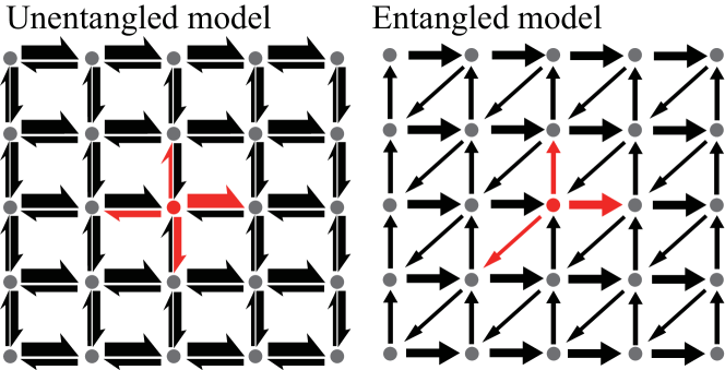
Figure A1: (Left) An “unentangled” lattice model $H$ can be decomposed into arrays of 1D chains , in this case into a vertical and a horizontal array of Hatano-Nelson models. As such, its full OBC properties can be correctly predicted with conventional GBZ theory, well-established for effectively 1D models. (Right) With additional couplings between different arrays of 1D chains, the lattice becomes “entangled” – the scenario for most realistic systems with longer-ranged effective couplings (shown here is the simplest possible case). Our dimensional transmutation approach is required to correctly characterize the full OBC system, as explained below and summarized in Fig. A2.

.1 Detailed walkthrough

We now walk through our general approach in detail, illustrating it with the model of Eq. 3 with $\alpha=b=2,\beta=a=1$, and summarized with flowcharts in Fig. A2. The starting point for a generic 2D model is its energy dispersion $E(z_{x},z_{y})$, where $z_{x}=\exp(ik_{x})$, $z_{y}=\exp(ik_{y})$ under periodic boundary conditions (PBCs), but would be complex deformed under OBCs.

Under $x$-OBC, we treat $E(z_{x},z_{y})$ as a 1D model with parameter $z_{y}$, and obtain the $x$-GBZ $z_{x}(k_{1},z_{y})$ via the conditionYao and Wang (2018); Zhang et al. (2020); Yokomizo and Murakami (2019). that every OBC energy $E(z_{x}(k_{1},z_{y}),z_{y})$ corresponds to at least two different $k_{1}$ solutions with identical inverse localization length $-\log|z_{x}(k_{1},z_{y})|$. To obtain the full OBC spectrum, the conventional approach would be to next implement $y$-OBCs, yielding $E(z_{x}(k_{1},z_{y}(k_{1},k_{2})),z_{y}(k_{1},k_{2}))$ (left column of Fig. A2). However, this may not correctly predict the full OBC spectrum in generic “entangled” lattices [Fig.2].

Instead, in our approach (middle & right columns of Fig. A2), we simultaneously obtain the $y$-GBZ $z_{y}(z_{x},k_{2})$ by treating $z_{x}$ as a parameter, and then obtain the provisional GBZ by simultaneously solving for $z_{x},z_{y}$ in terms of $k_{1},k_{2}$. Explicitly for our example described by

$$E(z_{x},z_{y})=t_{1}z_{x}^{2}z_{y}+t_{2}z_{x}^{-1}z_{y}+t_{3}z_{x}^{-1}z_{y}^{-2},$$ (A1)

the provisional GBZ is given by

$$\begin{split}\left\{\begin{array}[]{ll}z_{x}^{3}=\displaystyle\frac{t_{2}}{t_{1}}\frac{2\cos k_{1}+\text{e}^{3ik_{1}}}{4\cos k_{1}\cos k_{2}\text{e}^{-3ik_{2}}-\text{e}^{3ik_{1}}},\\ z_{y}^{3}=\displaystyle\frac{t_{3}}{t_{2}}\frac{4\cos k_{1}\cos k_{2}\text{e}^{-3ik_{1}}-\text{e}^{3ik_{2}}}{2\cos k_{2}+\text{e}^{3ik_{2}}},\end{array}\right.\ \end{split}$$ (A2)

such that the spectrum is deformed as $E(z_{x},z_{y})\rightarrow$

$$E(k_{1},k_{2})=\sqrt[3]{t_{1}t_{2}t_{3}}\frac{(2\cos 2k_{1}+1)^{\frac{2}{3}}(2\cos 2k_{2}+1)^{\frac{2}{3}}}{\left(\text{e}^{2ik_{1}}+\text{e}^{2ik_{2}}+1\right)^{\frac{1}{3}}}\text{e}^{{2in\pi}/{3}}$$ (A3)

with real $k_{1},k_{2}$ and solution branches $n=1,2,3$. Importantly, $E(k_{1},k_{2})$ should never possess nonzero spectral winding Okuma et al. (2020); Zhang et al. (2020), being an OBC spectrum. For many cases such as Eq.A3, it is however complex with nontrivial winding. Yet, $E(k_{1},k_{2})$ can be rigorously verified to satisfy all the model hopping constraints, and thus cannot be incorrect. Hence we conclude that the correct effective BZ consists of 1D subspaces of the provisional 2D GBZ. For generic $E(k_{1},k_{2})$ with nontrivial spectral winding, we stipulate that the 1D effective GBZ consists of paths parametrized by $k_{1}=f(k),k_{2}=g(k)$, such that $\bar{E}=E(f(k),g(k))$ has vanishing $k$-winding. Numerically, it indeed predicts the correct full OBC spectrum (bottom right of Fig. A2).

For our example, 1D paths given by $(k_{1},k_{2})=(2k,k)$ or $(k_{1},k_{2})=(k,2k)$, $k\in[-\pi,\pi)$ yield zero spectral winding, leading to two effective 1D GBZ sectors

$$\begin{split}&\text{GBZ}_{1}=\left\{z_{x,1}^{3}=\frac{t_{2}}{t_{1}}\text{e}^{ik},z_{y,1}^{3}=\frac{t_{3}}{t_{2}}\frac{1}{2\cos\left(k/3\right)-1}\right\},\\ &\text{GBZ}_{2}=\left\{z_{x,2}^{3}=\frac{t_{2}}{t_{1}}\left(2\cos\left(k^{\prime}/3\right)-1\right),z_{y,2}^{3}=\frac{t_{3}}{t_{2}}\text{e}^{-ik^{\prime}}\right\}\end{split}$$ (A4)

whose union $\text{GBZ}_{1}\cup\text{GBZ}_{2}$ forms the full effective BZ.

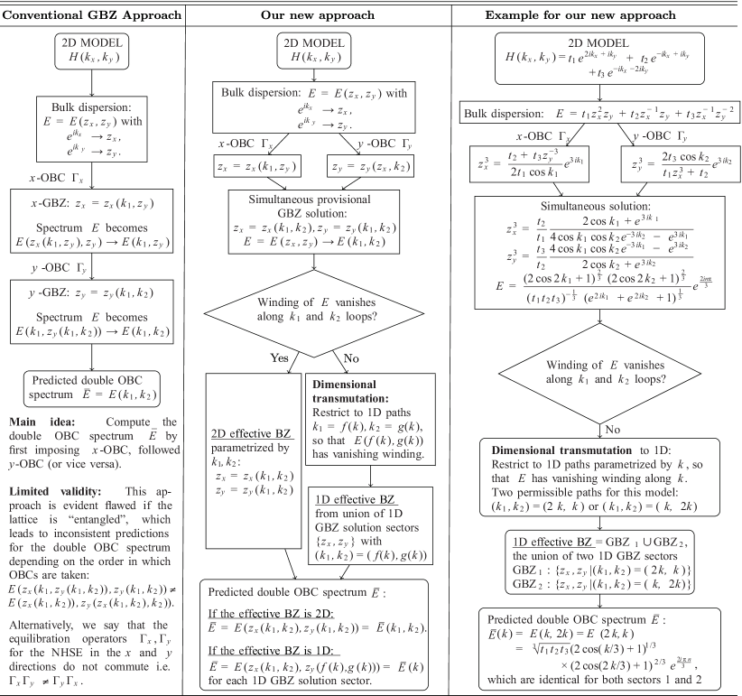
Figure A2: Summary of the key differences between our dimensional reduction approach and the conventional GBZ approach, accompanied by an illustrative example (Here we specialized to 2D, see Sect. V of  sup for higher-dimensional generalizations).

Instead of sequentially eliminating boundary conditions in the different directions, as in the conventional GBZ method, our new approach computes the double OBC spectrum $\bar{E}$ by first simultaneously imposing $x$- and $y$-OBCs, and obtaining their simultaneous solution. Then we check if the spectral winding vanishes: If yes, we are done; if not, perform the additional step of dimensional transmutation, reducing the 2D effective BZ to the union of 1D GBZ sectors consistent with vanishing spectral winding. As shown in [Fig.3(b)], the 1D-transmuted $\bar{E}(k)$ (light blue) agrees with the numerically obtained 2D OBC spectrum $E_{\text{OBC}}$ (blue circles), while the unconstrained $E(z_{x}(k_{1},k_{2}),z_{y}(k_{1},k_{2}))$ in the 2D GBZ gives the incorrect spectrum with extraneous eigenenergies (gray).

Our new approach is valid for all 2D lattices, whether entangled or unentangled. For its extension to higher dimensions, please refer to Sect. V of sup .

S1 I. Analytic GBZ results for generic 1D systems with two hopping terms

As a foundation for the analysis of the effective BZ of higher-dimensional lattices, we develop in this section a general analytic derivation for the generalized Brillouin zone (GBZ) results for 1D systems with 2 hopping terms, and compare them with numerics. In this supplement, we shall refer to “GBZ” and “effective BZ” interchangeably. Note that these results may no longer hold when there are more than 2 hopping terms, which is the more interesting scenario which this work is concerned with.

S1.1 Preliminaries

Consider the following 1D single-band model with dissimilar left/right hoppings:

$$\begin{split}H_{\text{1D}}=\sum_{n}A|n\rangle\langle n+\alpha|+B|n\rangle\langle n-\beta|\ ,\end{split}$$ (S1)

whose eigenvalues are $E(z)=Az^{\alpha}+Bz^{-\beta}$, where $z=\text{e}^{ik}$ describes the momentum component normal to the boundary of interest. This effective 1D single-band system has only 2 hoppings, one is to move $\alpha$ sites to the left by amplitude $A$, the other with amplitude $B$, $\beta$ sites to the right. In higher-dimensional contexts, $A$ and $B$ can depend on the momenta from the other directions.

Corresponding to this eigenvalue $E(z)=Az^{\alpha}+Bz^{-\beta}$ is the eigenstate $|\psi(z)\rangle$. In deference to Bloch’s theorem, we assume that it takes the form of a generalized Bloch state given by the ansatz $|\psi(z)\rangle=(...,\psi_{n}(z),...)^{\text{T}}$, $\psi_{n}(z)=z^{n}$, position index $n$, which satisfies the bulk equation

$$A\psi_{n+\alpha}(z)+B\psi_{n-\beta}(z)=E(z)\psi_{n}(z)\ .$$ (S2)

At a particular energy $E(z)$, there exists other wavefunction solutions $|\psi(z^{\prime})\rangle$ which satisfies the same eigenvalue $E(z)$, i.e.

$$\begin{split}&Az^{\prime\alpha}+Bz^{\prime-\beta}-E(z)=0\ .\end{split}$$ (S3)

This equation above is a polynomial relation of order $\alpha+\beta$ in $z$, and it’s easy to get its solutions $z_{1},z_{2},...,z_{\alpha+\beta}$, which can all be expressed in terms of $z$. These solutions shall provide information about how $z$ is controlled by hopping amplitudes $A$ and $B$.

Hereupon, an eigensolution $|\Psi\rangle$ with eigenenergy $E(z)$ can be written as

$$|\Psi\rangle=\sum^{\alpha+\beta}_{i=1}c_{i}|\psi(z_{i})\rangle\ ,$$ (S4)

with coefficients $c_{i}$ $(i=1,2,...,\alpha+\beta)$. To determine how they are constrained, we apply open boundary conditions onto $|\Psi\rangle$, arriving at

$$\Psi_{n^{\prime}}=\sum^{\alpha+\beta}_{i=1}c_{i}z_{i}^{n^{\prime}}=0\ ,\quad\quad n^{\prime}=0,-1,-2,...1-\beta\quad\text{or}\quad L+1,L+2,...L+\alpha\ ,$$ (S5)

that is, there have $\alpha+\beta$ constraints from the open boundary conditions (OBCs), which together combine to form the GBZ characteristic equation

$$\text{det}\ M=\sum^{\alpha+\beta}_{n_{1},n_{2},...n_{\alpha+\beta}=1}\varepsilon_{n_{1},n_{2},...,n_{\alpha+\beta}}z_{n_{1}}^{1-\beta}\times z_{n_{2}}^{2-\beta}\times...\times z_{n_{\beta}}^{0}\times z_{n_{\beta+1}}^{L+1}\times z_{n_{\beta+2}}^{L+2}\times...\times z_{n_{\alpha+\beta}}^{L+\alpha}=0\ ,$$ (S6)

where the matrix $M$ is $(\alpha+\beta)\times(\alpha+\beta)$ square array , $\varepsilon_{n_{1},n_{2},...,n_{\alpha+\beta}}$ is $\alpha+\beta$-order arrangement, and $\varepsilon_{n_{1},n_{2},...,n_{\alpha+\beta}}=-1$, when $n_{1},n_{2},...,n_{\alpha+\beta}$ is odd arrangement, $\varepsilon_{n_{1},n_{2},...,n_{\alpha+\beta}}=1$ if $n_{1},n_{2},...,n_{\alpha+\beta}$ is even arrangement. Since $z_{1},z_{2},...,z_{\alpha+\beta}$ are all functions of $z$, the GBZ characteristic equation Eq.(S6) is in actuality only a function of $z$.

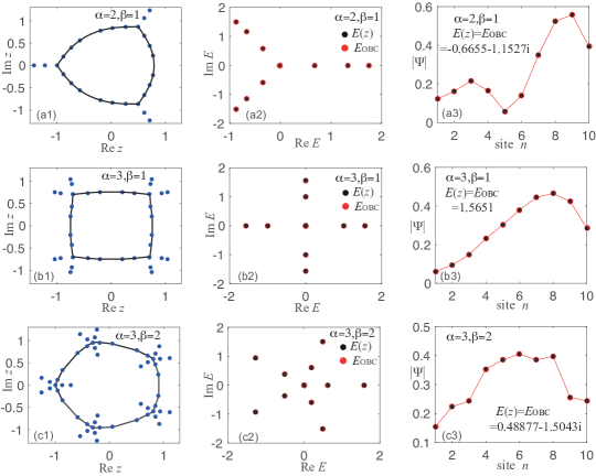
Figure S1: (a1–c1) Solutions $z$ to the characteristic equation (Eq.(S6)) for a few illustrative values of $\alpha,\beta$, with $A=B=1$ and system size of $L=10$ sites. Blue dots represent the full set of solutions, but only those lying on the black constraint curves constitute the actual GBZ solutions for OBCs. (a2–c2) Their corresponding eigenenergies $E(z)=Az^{\alpha}+bz^{-\beta}$ (black) are the set of $z$ points belonging to the GBZ, which agree excellently with $E_{\text{OBC}}$ (red) of Eq.(S1). (a3–c3) shows the excellent agreement between numerical eigenstate solutions (red) and their corresponding GBZ solutions (black).

Taking the model Eq.(S1) with $\alpha=2,\beta=1$ as a sample, the eigenvalues $E(z)=Az^{2}+B/z$ can be obtained by bulk equation Eq.(S6). Considering the same eigenenergy $E(z)$, the eigensolution $|\Psi\rangle$ can be written as $|\Psi\rangle=\sum_{i=1}^{3}c_{i}|\psi(z_{i})\rangle$, $\psi_{n}(z_{i})=z_{i}^{n}$, and $z_{i}$ which satisfy $Az_{i}^{2}+B/z_{i}-E(z)=0$, are constrained by $z$ and hopping amplitude $A,B$

$$z_{1}=z\ ,\ z_{2}=-\frac{z}{2}+\sqrt{\frac{B}{Az}+\frac{z^{2}}{4}}\ ,\ z_{3}=-\frac{z}{2}-\sqrt{\frac{B}{Az}+\frac{z^{2}}{4}}\ .$$ (S7)

Applying open boundary conditions into $|\Psi\rangle$, we can get GBZ characteristic equation

$$\begin{split}\text{det}\ M=\text{det}\begin{pmatrix}1&1&1\\ z_{1}^{L+1}&z_{2}^{L+1}&z_{3}^{L+1}\\ z_{1}^{L+2}&z_{2}^{L+2}&z_{3}^{L+2}\end{pmatrix}=(z_{1}z_{2})^{L+1}(z_{2}-z_{1})+(z_{1}z_{3})^{L+1}(z_{1}-z_{3})+(z_{2}z_{3})^{L+1}(z_{3}-z_{2})=0\ ,\end{split}$$ (S8)

which is only a function of $z$. The determinant must vanish so that we have a nontrivial eigenstate solution $(c_{1},c_{2},c_{3})^{\text{T}}$ of the matrix $M$ with eigenvalue $0$. It is worth noting that not all the solution $z$ of GBZ characteristic equation Eq.(S8) is GBZ results of the system, as show in FIG. S1(a1—a3). To put it simply, for fixed $z$, $z_{1},z_{2},z_{3}$ which are from Eq.(S7) can be rearranged by $|z_{1}|\leq|z_{2}|\leq|z_{3}|$. If the absolute value $|z_{3}|$ is not equal to $|z_{2}|$, we have $\lim\limits_{L\gg 1}c_{3}=0,(c_{1}=-c_{2})$, that is, the solution $z_{3}$ does not belong to GBZ. And in other cases, we can also select GBZ solutions from the set of solution $z$ by the values of the coefficients $c_{1},c_{2},c_{3}$.

S1.2 Determination of the GBZ for OBCs

However, not all solutions $z$ of the characteristic equation Eq.(S6) contribute to the actual OBC solutions. Those that do define the GBZ. In Figs. S1(a1—c1), we see that of all solutions $z$ (blue dots), only those that lie on the black curves correspond to values of $E(z)$ that coincide with actual numerically obtained eigenvalues (Figs. S1(a2—c2)).

From known results on GBZ construction Lee and Thomale (2019); Yang et al. (2020); Lee et al. (2020a), solutions $z$ that belong to the GBZ (i.e. black curves) are those $z$ such that there exists another $z^{\prime}\neq z$ such that $|z|=|z^{\prime}|$ and $E(z)=E(z^{\prime})$. If more than one such pair of solutions exist, the GBZ is defined by the pair with $|z|=|z^{\prime}|$ closest to unity. This is because $|z|$ determines the spatial decay rate of the eigensolution, and the GBZ pair is given by the pair of solutions that are mostly slowly decaying, and yet able to satisfy OBCs at both boundaries (which can be arbitrarily far) simultaneously. In other words, the GBZ is obtained through the pair among $z_{1},z_{2},...,z_{\alpha+\beta}$ with the same absolute value.

Let’s now solve for the GBZ of our 1D lattice $H_{\text{1D}}$, with $z$ parametrized by a wavenumber $k$. First, we write the two degenerate (equal energy) solutions of $z$ as $z_{\pm}=z_{0}\text{e}^{ik^{\prime}\pm k}$, with real $k^{\prime},k$ and possessing the same energy $E(z_{\pm})$. Here $z_{0}$ is a parameter that is unspecified for now. Taking $z_{\pm}$ into the energy equation,

$$\begin{split}E=E(z_{+})=E(z_{-})=Az_{0}^{\alpha}\text{e}^{i\alpha(k^{\prime}+k)}+Bz_{0}^{-\beta}\text{e}^{i\beta(k^{\prime}+k)}=Az_{0}^{\alpha}\text{e}^{i\alpha(k^{\prime}-k)}+Bz_{0}^{-\beta}\text{e}^{-i\beta(k^{\prime}-k)}\ .\end{split}$$ (S9)

As such, we can solve for $z_{\pm}$:

$$\begin{split}z_{\pm}&=\left(\frac{B\sin\beta k}{A\sin\alpha k}\right)^{\frac{1}{\alpha+\beta}}\text{e}^{\pm ik+i\frac{2\pi v}{\alpha+\beta}}\ ,\\ \end{split}$$ (S10)

with $v=1,2,...,\alpha+\beta$. Note that $|z_{\pm}|\neq 1$ in general, and only when $k=n\pi/(\alpha+\beta)$ do we have $|\sin\beta k|/|\sin\alpha k|=1$. Due to the periodicity of $2\pi/(\alpha+\beta)$, without loss of generality, we shall from now on set the range of parameter $k$ to be $[n\pi-\pi/(\alpha+\beta),n\pi+\pi/(\alpha+\beta))$, with integer $n$. For definiteness, we take $n=0$.

In all, the GBZ of our model $H_{\text{1D}}$ (Eq.(S1)) is given by

$$\text{GBZ}_{\text{1D}}=\left\{z=\left(\left.\frac{B\sin\beta k}{A\sin\alpha k}\right)^{\frac{1}{\alpha+\beta}}\text{e}^{ik+i\frac{2\pi v}{\alpha+\beta}}\,\right|k=\left(-\frac{\pi}{\alpha+\beta},\frac{\pi}{\alpha+\beta}\right],v=1,2,..\alpha+\beta\right\}\ ,$$ (S11)

giving energies

$$\begin{split}\bar{E}(k)=E(z)&=Az^{\alpha}+Bz^{-\beta}=\left(\frac{A^{\beta}B^{\alpha}}{(\sin(\alpha k))^{\alpha}(\sin(\beta k))^{\beta}}\right)^{\frac{1}{\alpha+\beta}}\sin\left((\alpha+\beta)k\right)\text{e}^{\frac{2i\pi\alpha v}{\alpha+\beta}}\ ,\end{split}$$ (S12)

which agrees closely with numerical OBC eigenenergies in Figs. S1(a2—c2). Here, the bar above $\bar{E}(k)$ indicates that the energy function is evaluated on the GBZ, i.e. it depends on $k$ not on the ordinary BZ, but through the GBZ. Previously, it was already conceived that complex momentum can be used to represent state decay Kohn (1959); He and Vanderbilt (2001); Lee and Ye (2015), but in this GBZ formalism, the imaginary part of the momentum is specifically solved to give the profile of OBC eigenstates. Eq. S11 is a main result that will be used in the GBZ computation of higher-dimensional cases later on. As consistent with the fact that OBC spectra cannot undergo any further NHSE (in the same direction), the spectral winding of $E(z)$ above is always zero, that is, the distribution of $E(z)$ in the complex plane cannot form closed curves.

In generic 1D lattices with multiple hopping terms, Eq. S9 will have to be replaced by a simultaneously polynomial relations which has to be solved numerically. The resultant GBZ is still well-defined, although it is likely obtainable only numerically.

S2 II. 2D non-Hermitian lattices with 2D GBZs

This section introduces how the GBZ can be obtained for 2D lattices through a few concrete examples with different hopping terms.

The Schrödinger equation in periodic 2D potential $U(\bm{r}+\bm{r}^{\prime}_{nm})=U(\bm{r})$ with $\bm{r}^{\prime}_{nm}=(nd,md^{\prime})$ and lattice period $d$,$d^{\prime}$ reads

$$H\psi(\bm{r})=(-\partial^{2}+U(\bm{r}))\psi(\bm{r})=E\psi(\bm{r})\ ,$$ (S13)

where $\psi(\bm{r})=\sum_{nm}c_{nm}\phi(\bm{r}-\bm{r}^{\prime}_{nm})$, $\bm{r}=(x,y)$. Assume $\phi(\bm{r})$ is the eigen-wave-function of Hamiltonian $H_{0}$ with single atom potential $V(\bm{r})$(consider only one state)

$$H_{0}\phi(\bm{r})=(-\partial^{2}+V(\bm{r}))\phi(\bm{r})=E_{0}\phi(\bm{r})\ ,$$ (S14)

Define $\delta U(\bm{r})=U(\bm{r})-V(\bm{r})$, and substitute following equation

$$H\psi(\bm{r})=(H_{0}+\delta U(\bm{r}))\psi(\bm{r})=E\psi(\bm{r})\ ,$$ (S15)

and

$$\sum_{n,m}\langle\phi_{n^{\prime}m^{\prime}}|\delta U(\bm{r})|\phi_{nm}\rangle c_{nm}=(E-E_{0})c_{n^{\prime}m^{\prime}}\ ,$$ (S16)

with $\phi_{nm}=\phi(\bm{r}-\bm{r}^{\prime}_{nm})$. Define: $\langle\phi_{n^{\prime}m^{\prime}}|\delta U(\bm{r})|\phi_{nm}\rangle=-J(\bm{r}^{\prime}_{nm}-\bm{r}^{\prime}_{n^{\prime}m^{\prime}})$ and

$$-\sum_{n,m}J(\bm{r}^{\prime}_{nm}-\bm{r}^{\prime}_{n^{\prime}m^{\prime}})c_{nm}=(E-E_{0})c_{n^{\prime}m^{\prime}}.$$ (S17)

Because of the tranformation symmetry of the Hamiltonian, the resulting wavefunction $\psi(\bm{r})$ should take Bloch form, which means we should have the solution $c_{nm}=\exp(i\bm{k}\bm{r}^{\prime}_{nm})$

$$E-E_{0}=-\sum_{n,m}J(\bm{r}^{\prime}_{nm})\exp(-i\bm{k}\bm{r}^{\prime}_{nm})\ .$$ (S18)

if consider the specific hoppings, define $J_{0}=J(\bm{0}),J_{nm}=J(\pm\bm{r}^{\prime}_{nm})$, then we have

$$E-E_{0}+J_{0}=\sum_{nm}J_{nm}\exp(-i\bm{k}\bm{r}^{\prime}_{nm})$$ (S19)

In the second quantization language, the expectation value of energy becomes a operator, set $H=-\partial^{2}+U(\bm{r})$, we have

$$\hat{H}=\sum_{nm,n^{\prime}m^{\prime}}\hat{c}^{\dagger}_{nm}H_{nm,n^{\prime}m^{\prime}}\hat{c}_{n^{\prime}m^{\prime}}$$ (S20)

with $\psi\rightarrow\hat{\psi}=\sum\hat{c}_{nm}\psi_{nm}$, $H_{nm,n^{\prime}m^{\prime}}=\langle\phi_{n^{\prime}m^{\prime}}|H|\phi_{nm}\rangle$, $\phi_{nm}$ is a orthonormal and complete basis in Hilbert space, like plane-waves $\exp(i\bm{k}\bm{r})$ or energy eigen-states of $H_{0}$, $H$ is the energy operator in single particle first quantization picture, which can only act on Hilbert space, while the second quantization energy operator $\hat{H}$ acts on Fock space. Here, in tight-binding method, $\phi_{nm}$ is the wave-function of site $\bm{r}^{\prime}_{nm}$ of the energy eigen-state $H_{0}$. Consider the specific hoppings, we have

$$\hat{H}=\sum_{nm}J_{\alpha,\beta}\hat{c}^{\dagger}_{n+\alpha,m+\beta}\hat{c}_{n,m}\ ,$$ (S21)

results in a simple Hamiltonian and allows for quick computations. And in our manuscript, all the hamiltonian second quantization formulation.

S2.1 2D lattice model with 2 hopping terms

To connect with our previous treatment of 1D lattices with 2 hopping terms, we first consider the simplest case of 2D lattices with 2 hopping terms:

$$H_{\text{2D,2}}=\sum_{m,n}t|m,n\rangle\langle m+\alpha,n+a|+t^{\prime}|m,n\rangle\langle m-\beta,n-b|\ ,$$ (S22)

with hoppings of amplitudes $t$ (or $t^{\prime}$) corresponding to transitions of $(-\alpha,-a)$ sites ( or $(\beta,b)$ sites) on the lattice.

We consider the ansatz $|\psi\rangle\propto\sum_{m,n}\psi_{mn}|m,n\rangle$ with $\psi_{mn}=z_{x}^{m}z_{y}^{n}$. In the bulk, it gives eigenenergies $E(z_{x},z_{y})$

$$E(z_{x},z_{y})=tz_{x}^{\alpha}z_{y}^{a}+t^{\prime}z_{x}^{-\beta}z_{y}^{-b}.$$ (S23)

For a fixed $z_{x}$, there are $a+b$ solutions $z_{y,i}$, ($i=1,2,...,a+b$) corresponding to the same energy $E(z_{x},z_{y})$. Similarly, we can also find $\alpha+\beta$ solutions $z_{x,j}$, ($j=1,2,...,\alpha+\beta$) corresponding to fixed $E(z_{x},z_{y})$ and $z_{y}$. Both sets of solutions $z_{y,i}$, ($i=1,2,...,a+b$) and $z_{x,j}$, ($j=1,2,...,\alpha+\beta$) can be written entirely in terms of $z_{x}$ and $z_{y}$.

We next show a detailed for derivation of the GBZ of $H_{\text{2D,2}}$. For a quick heuristic approach, the reader may directly skip to Eqs. S25 and S26.

Implementing open boundary conditions on the wavefunction $|\Psi\rangle$ for a fixed eigenenergy $E(z_{x},z_{y})$ gives

$$\begin{split}|\Psi\rangle=|\Psi^{1}\rangle=|\Psi^{2}\rangle\ \propto\sum_{m,n}\Psi_{mn}|m,n\rangle=\sum_{m,n}\Psi^{1}_{mn}|m,n\rangle=\sum_{m,n}\Psi^{2}_{mn}|m,n\rangle\ ,\\ \quad\Psi^{1}_{mn}=\sum_{z_{y}}\left(\left(\sum_{j}^{\alpha+\beta}f_{z_{x,j}}z_{x,j}^{m}\right)g_{z_{y}}z_{y}^{n}\right)\ ,\quad\Psi^{2}_{mn}=\sum_{z_{x}}\left(f_{z_{x}}z_{x}^{m}\left(\sum_{i}^{a+b}{g}_{z_{y,i}}z_{y,i}^{n}\right)\right)\ ,\\ \end{split}$$ (S24)

Here, we have written $|\Psi\rangle$ either as $|\Psi^{1}\rangle$ or $|\Psi^{2}\rangle$, depending on the order of expansion in terms of the $x$ and $y$ coefficients. These two ways to expand are of course equivalent, and note the relation $f_{z_{x}}g_{z_{y,i}}=g_{z_{y,i}}f_{z_{x}}$. The $\sum_{i},\sum_{j}$ summations in $\Psi^{1}_{mn},\Psi^{2}_{mn}$ refers to sums over all sets $z_{x},z_{y}$ which have same energy $E$. To treat boundary conditions along different direction (i.e.,${\bm{x},\bm{y}}$ directions), we can choose the appropriate expansion and proceed like in the 1D case (see Sec. S1), paying careful attention to the indices i.e. for OBCs along the ${\bm{x}}$ direction, we have $\Psi_{m^{\prime}{n}}=\Psi^{1}_{m^{\prime}{n}}=0$ for any $n$ and $m^{\prime}=-\beta+1,-\beta+2,...0,L+1,L+2,..L+\alpha$ (assuming $\alpha,\beta>0$). Thus we obtain

$$\begin{split}z_{x}^{\alpha+\beta}=\frac{t^{\prime}}{t}\frac{z_{1}^{\alpha+\beta}}{z_{y}^{a+b}},\quad z_{1}^{\alpha+\beta}=\frac{\sin\beta k_{1}}{\sin\alpha k_{1}}\text{e}^{i(\alpha+\beta)k_{1}}\ ,\end{split}$$ (S25)

with momentum parameter $k_{1}\in\left(-\frac{\pi}{\alpha+\beta},\ \frac{\pi}{\alpha+\beta}\right]$ as in a quasi-1D case (see Sec. S1. for details). Likewise, considering the expansion via $|\Psi\rangle=|\Psi^{2}\rangle$ with boundary conditions along the ${\bm{y}}$ direction, we obtain the alternative expressions

$$\begin{split}z_{y}^{a+b}=\frac{t^{\prime}}{t}\frac{z_{2}^{a+b}}{z_{x}^{\alpha+\beta}},\quad z_{2}^{a+b}=\frac{\sin bk_{2}}{\sin ak_{2}}\text{e}^{i(a+b)k_{2}}\ ,\end{split}$$ (S26)

with $k_{2}\in\left(-\frac{\pi}{a+b},\ \frac{\pi}{a+b}\right]$. To solve for the GBZs of simultaneous x-OBCs and y-OBCs in 2D, we simultaneously solve Eqs. S25 and S26. Note that heuristically, Eqs. S25 and S26 can be simply written down by treating $H_{\text{2D,2}}$ as a 1D chain with hoppings dependent on the transverse momentum. For instance, we can write Eq. S23 either as $E(z_{x})=(tz_{y}^{a})z_{x}^{\alpha}+(tz_{y}^{-b})z_{x}^{-\beta}$ or $E(z_{y})=(tz_{x}^{\alpha})z_{y}^{a}+(tz_{x}^{-\beta})z_{y}^{-b}$, and apply Eq. S11 to obtain Eqs. S25 and S26 respectively. Importantly, we shall see that this approach fails in general 2D lattices, even though it is valid in this case where there are only two hopping terms from each site.

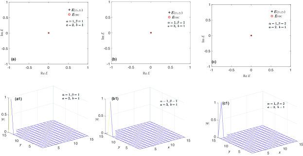
Figure S2: Spectra and corner-localized eigenstates for $H_{\text{2D,2}}$ in the $\alpha/\beta\neq a/b$ case. (a–c) Exactly zero (flatband) OBC eigenenergies $E_{\text{OBC}}$ due to non-Bloch collapse, which coincide with $E(z_{x},z_{y})$ from Eq.(S28). (a1—c1) Corresponding illustrative eigenstates are perfectly localized at the boundary dictated by the direction of localization. The model parameters are $L_{x}=L_{y}=15$, $t=2,\quad t^{\prime}=1$ and the specific values of $\alpha,\beta,a,b$ are indicated in the figure.

In the following, we shall specialize to the case where the two hoppings are pointing in the same direction i.e. $\alpha/\beta=a/b$, for reasons that will be become evident soon. In this case, the GBZ and energy satisfy

$$\begin{split}&\text{GBZ}_{\text{2D,2}}=\left\{\left.z_{x}^{\alpha+\beta}z_{y}^{a+b}=\frac{t^{\prime}\sin bk}{t\sin ak}\text{e}^{i(a+b)k}\right|k=\left(-\frac{\pi}{a+b},\frac{\pi}{a+b}\right]\right\}\ ,\\ &\bar{E}(k)=E(z_{x},z_{y})=\left(\frac{t^{b}t^{\prime a}}{(\sin(ak))^{a}(\sin(bk))^{b}}\right)^{\frac{1}{a+b}}\sin\left((a+b)k\right)\text{e}^{\frac{2i\pi av}{a+b}}\ ,\end{split}$$ (S27)

with $k=\left(-\frac{\pi}{a+b},\frac{\pi}{a+b}\right]$ and $v=1,2,...,a+b$, as plotted in FIG. S3 (a—c). As this case only contains the combination $z_{x}^{\alpha+\beta}z_{y}^{a+b}$, rather than $z_{x}^{\alpha+\beta}$ and $z_{y}^{a+b}$, it is essentially a 1D model along the $\alpha\bm{x}+a\bm{y}$ direction, which is consistent with the results of numerical diagonalization as shown in FIG. S3(a1—a3).

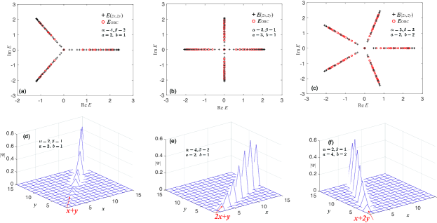
Figure S3: Spectra and illustrative eigenstates for $H_{\text{2D,2}}$ in the $\alpha/\beta=a/b$ case. (a–c) Excellent agreement between the GBZ eigenenergies $E(z_{x},z_{y})$ from Eq.(S27) and OBC eigenenergies $E_{\text{OBC}}$ of Eq.(S22). (d–f) Spatial profiles for the $E_{\text{OBC}}=0$ eigenstate of a few other illustrative cases, clearly showing that the skin states are aligned along the $\alpha\hat{x}+a\hat{y}$ (or $\beta\hat{x}+b\hat{y}$) direction. The model parameters are $L_{x}=L_{y}=15$, $t=1,\ t^{\prime}=2$ and the specific values of $\alpha,\beta,a,b$ are indicated in the figure.

We next discuss the other case with $\alpha/\beta\neq a/b$, where $|z_{1}|$ and $|z_{2}|$ can only coincide at $z_{1}^{\alpha+\beta}=z_{2}^{a+b}=-1$. Hereby, its GBZ and energy are simply given by

$$\begin{split}&\text{GBZ}_{\text{2D,2}}=\left\{z_{x}^{\alpha+\beta}z_{y}^{a+b}=-\frac{t^{\prime}}{t}\right\}\ ,\\ &\qquad\qquad\quad E(z_{x},z_{y})=0\ ,\end{split}$$ (S28)

As confirmed in FIG. S2(a–c), the eigenenergies are indeed zero, and the eigenstates (FIG. S2(a1–c1)) are perfectly localized at a corner determined by $\alpha/\beta$, $a/b$ and $t/t^{\prime}$. This is because of uncompensated unbalanced hoppings along at least one direction, which leads to non-Bloch collapse Longhi (2020); Crespi et al. (2013). Since there is no nontrivial dynamics to speak of in this case, we shall not discuss it further.

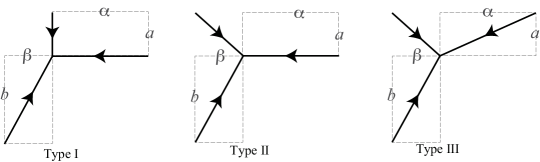
Figure S4: The three directed hopping configurations in each of our type I,II and III models. For type I, two hoppings are orthogonal; for type II, two hoppings have common $\beta$ displacements in the direction antiparallel to the third hopping; for type III, there exists two common $\beta$ component displacements orthogonal to the two common $a$ displacements.

S2.2 2D lattice model with 3 hopping terms

We next discuss 2D lattices with 3 unbalanced hopping terms, such that their combined effect is no longer either trivial or just that along a 1D subspace. We shall study two types of hopping configurations here, and reserve the third type, which turns out to interestingly requires a GBZ of lower dimensionality, to the next section on its own.

S2.2.1 Type I: 2D lattice model with 3 hopping terms, 2 perpendicular to each other

We first consider type I models, the simplest of “entangled” 2D lattice models. They contain 2 perpendicular terms $t_{1},t_{2}$ in directions $(\alpha,0)$ and $(0,a)$, and a third one in an oblique direction $-(\beta,b)$. We have

$$H_{\text{2D,I}}=\sum_{m,n}t_{1}|m,n\rangle\langle m+\alpha,n|+t_{2}|m,n\rangle\langle m,n+a|+t_{3}|m,n\rangle\langle m-\beta,n-b|\ .$$ (S29)

Similarly as before, by substituting the ansatz $|\psi\rangle\propto\sum_{m,n}\psi_{mn}|m,n\rangle$ with $\psi_{m,n}=z_{x}^{m}z_{y}^{n}$ into the bulk equations, we obtain the energy $E(z_{x},z_{y})$

$$E(z_{x},z_{y})=t_{1}z_{x}^{\alpha}+t_{2}z_{y}^{a}+t_{3}z_{x}^{-\beta}z_{y}^{-b}\ .$$ (S30)

By heuristically regarding $E(z_{x},z_{y})$ as 1D models $E(z_{x})$ or $E(z_{y})$ with nonconstant hoppings and using Eqs. S11 and S12, or by considering boundary conditions on the wave function $|\Psi\rangle$ (Eq.(S24)), we obtain the following relationships between $z_{x}$ and $z_{y}$:

$$\begin{split}z_{x}^{\alpha+\beta}z_{y}^{b}&=\frac{t_{3}}{t_{1}}z_{1}^{\alpha+\beta},\quad z_{1}^{\alpha+\beta}=\frac{\sin\beta k_{1}}{\sin\alpha k_{1}}\text{e}^{i(\alpha+\beta)k_{1}},\ k_{1}\in\left(-\frac{\pi}{\alpha+\beta},\ \frac{\pi}{\alpha+\beta}\right]\ ,\\ z_{x}^{\beta}z_{y}^{a+b}&=\frac{t_{3}}{t_{2}}z_{2}^{a+b},\quad\ z_{2}^{a+b}=\frac{\sin bk_{2}}{\sin ak_{2}}\text{e}^{i(a+b)k_{2}},\quad k_{2}\in\left(-\frac{\pi}{a+b},\ \frac{\pi}{a+b}\right]\ .\end{split}$$ (S31)

Substituting these $z_{x}$ and $z_{y}$ into the energy expression Eq.(S30), we obtain the GBZ energies (Note the slight abuse of notation - below, we write $E(z_{x},z_{y})=E(z_{1},z_{2})$ to convey that the set of $E$ depends on $z_{1},z_{2}$ through $z_{x},z_{y}$, even though $E$ of course takes different functional dependencies in either case. )

$$\begin{split}\bar{E}(k_{1},k_{2})=E(z_{x},z_{y})&=\left(\frac{t_{1}^{\beta a}t_{2}^{\alpha b}t_{3}^{\alpha a}}{z_{1}^{(\alpha+\beta)a\beta}z_{2}^{(a+b)b\alpha}}\right)^{\frac{1}{(\alpha+\beta)a+\alpha b}}\times\left(1+z_{1}^{\alpha+\beta}+z_{2}^{a+b}\right)\ ,\\ \end{split}$$ (S32)

and

$$\begin{split}\text{GBZ}_{\text{2D,I}}=\left\{z_{x},z_{y}\left|z_{x}^{(\alpha+\beta)a+\alpha b}=\frac{t_{2}^{b}t_{3}^{a}}{t_{1}^{a+b}}\frac{z_{1}^{(\alpha+\beta)(a+b)}}{z_{2}^{(a+b)b}}\ ,\,z_{y}^{(\alpha+\beta)a+\alpha b}=\frac{t_{1}^{\beta}t_{3}^{\alpha}}{t_{2}^{\alpha+\beta}}\frac{z_{2}^{(\alpha+\beta)(a+b)}}{z_{1}^{(\alpha+\beta)\beta}}\right.\right\}\ ,\end{split}$$ (S33)

with $z_{1},z_{2}$ functions of $k_{1},k_{2}$, as defined in Eq.(S31). Some comments on the relationship between $z_{x},z_{y}$ and $z_{1},z_{2}$ are in order. As defined by the ansatz $|\psi(x,y)\rangle\propto\sum_{m,n}z_{x}^{m}z_{y}^{n}|m,n\rangle$, $z_{x},z_{y}$ control the spatial growth and decay of the wavefunction. However, unlike in an “unentangled” case like $H_{\text{2D,2}}$, both $z_{x}$ and $z_{y}$ depend on the GBZ spanning parameters $k_{1},k_{2}$ in complicated manners given by Eq. S31. In other words, Eq. S31 dictates how the “non-Bloch” scaling factors $z_{x},z_{y}$ are related to the GBZ coordinates $k_{1},k_{2}$ through intermediate quantities $z_{1},z_{2}$, which are related to the effective 1D chain projections of the Hamiltonian.

From this explicit expression Eq. S33, we can already deduce that the locus of $E$ is a star-like set of branches, since $E$ factorizes into a product of terms involving the phase factors of $k_{1}$ and $k_{2}$ separately. By considering these phase factors, we find that the number of branches for a type-I hopping lattice is given by

$$\text{LCM}\left[\displaystyle\frac{(\alpha+\beta)a+\alpha b}{\text{GCD}((\alpha+\beta)a+\alpha b,(\alpha+\beta)a\beta)},\displaystyle\frac{(\alpha+\beta)a+\alpha b}{\text{GCD}((\alpha+\beta)a+\alpha b,(a+b)\alpha b)}\right].$$ (S34)

Their agreement with numerical OBC results is given in FIG. S5. The phase factor is given by $\exp(\frac{2\pi i((\alpha+\beta)a\beta k_{1}+(a+b)\alpha bk_{2}}{(\alpha+\beta)a+\alpha b})$, which evaluates to $\exp(\frac{2\pi i(2k_{1}+2k_{2})}{3})\Leftrightarrow 3$ branches for (a4); $\exp(\frac{2\pi i(3k_{1}+4k_{2})}{5})\Leftrightarrow 5$ branches for (b4); and $\exp(\frac{2\pi(3k_{1}+12k_{2})}{7})\Leftrightarrow 7$ branches for (c4).

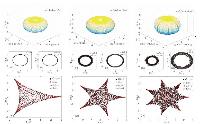
Figure S5: Plots of the GBZ torus (Upper row a1-c1) , GBZs $z_{x}$ (Middle row a2-c2) and $z_{y}$ (Middle row a3-c3), as well as the energy spectra (Lower row a4-c4) of illustrative type-I lattices ($H_{\text{2D,I}}$ from Eq. (S29)) with hoppings given by parameters $\alpha,\beta,a,b$. The upper row plots (a1-c1) are parametrized such that a torus is traced out in the trivial case without NHSE ($|z_{x}|=|z_{y}|=1$ for all $k_{1},k_{2}$); departures from a toroidal shape depict the extent of 2D NHSE. Belonging to a 2D model, each of $z_{x},z_{y}$ (a1-c1,a2-c2,a3-c3,) traces out a 2D region parametrized by $k_{1},k_{2}$ (Eq. S33) as its GBZ, even though it trivially collapses into 1D loops for case (a). Perfect agreement of GBZ spectra $E(z_{x},z_{y})$ from Eq. (S32) with OBC spectra $E_{\text{OBC}}$ is demonstrated for all cases, which for this model fills the interior of a $[(\alpha+\beta)a+\alpha b]$-sided figure (a4-c4). Parameters are $L_{x}=L_{y}=15$, $t_{1}=t_{1}=t_{3}=1$, and the GBZ predictions are generated with a mesh defined by $k_{1}=-\frac{\pi}{\alpha+\beta}:\frac{\pi}{30}:\frac{\pi}{\alpha+\beta}$, $k_{2}=-\frac{\pi}{a+b}:\frac{\pi}{30}:\frac{\pi}{a+b}$.

S2.2.2 Type II: 2D lattice model with 3 hopping terms, two with common $\beta$ displacement

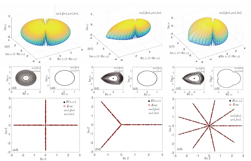
Figure S6: Plots of the GBZ torus (Upper row a1-c1) , GBZs $z_{x}$ (Middle row a2-c2) and $z_{y}$ (Middle row a3-c3), as well as the energy spectra (Lower row a3-c3)of illustrative type-II lattices ($H_{\text{2D,II}}$ from Eq. (S35)) with hoppings given by parameters $\alpha,\beta,a,b$. (a1-c1,a2-c2,a3-c3) While $z_{x}$ traces out a 2D region parametrized by the two “momenta” $k_{1}$ and $k_{2}$, $z_{y}$ only depends on one such momentum parameter, as given by Eq. (S37)), thereby tracing out a 1D GBZ loop (a3-c3). (a4-c4) Perfect agreement of GBZ spectra $E(z_{x},z_{y})$ from Eq. (S36) with OBC spectra $E_{\text{OBC}}$ is demonstrated for all cases, with their star-like spectra consistent with the 1D nature of their effective GBZ description. The $|z_{x}|=0$ central dot corresponds to $k_{2}=\pm\pi/(a+b)$ where the factor $\left(z_{2}^{a}+z_{2}^{-b}\right)$ in $z_{x}$ is equal to 0. Parameters are $L_{x}=L_{y}=15$, $t_{1}=t_{1}=t_{3}=1$, and the GBZ predictions are generated with a mesh defined by $k_{1}=-\frac{\pi}{\alpha+\beta}:\frac{\pi}{30}:\frac{\pi}{\alpha+\beta}$, $k_{2}=-\frac{\pi}{a+b}:\frac{\pi}{30}:\frac{\pi}{a+b}$.

We next consider a slightly more complicated 2D lattice model (type II). None of the hoppings are orthogonal to each other, so all 3 hoppings are “entangled”. However, it has the simplifying property that the $t_{2}$ and $t_{3}$ hoppings are equidistant in the direction parallel to the $t_{1}$ hopping, such that if we set the $t_{1}$ hopping normal against the horizontal $x$ open boundary, there are only two unique hopping distances in this direction. The Hamiltonian is given by

$$H_{\text{2D,II}}=\sum_{m,n}t_{1}|m,n\rangle\langle m+\alpha,n|+t_{2}|m,n\rangle\langle m-\beta,n+a|+t_{3}|m,n\rangle\langle m-\beta,n-b|\ .$$ (S35)

Taking the ansatz $|\psi\rangle\propto\sum_{m,n}\psi_{mn}|m,n\rangle$ with $\psi_{m,n}=z_{x}^{m}z_{y}^{n}$ into the bulk equations, we obtain the energy $E(z_{x},z_{y})$

$$E(z_{x},z_{y})=t_{1}z_{x}^{\alpha}+t_{2}z_{x}^{-\beta}z_{y}^{a}+t_{3}z_{x}^{-\beta}z_{y}^{-b}\ .$$ (S36)

Considering the boundary conditions in the same way as before, we have two relations between $z_{x}$ and $z_{y}$ from which the GBZ and OBC energy $E(z_{x},z_{y})$ can be obtained:

$$\begin{split}\text{GBZ}_{\text{2D,II}}=\left\{z_{x},z_{y}\left|z_{x}^{\alpha+\beta}=t_{1}^{-1}t_{2}^{\frac{b}{a+b}}t_{3}^{\frac{a}{a+b}}\left(z_{2}^{a}+z_{2}^{-b}\right)z_{1}^{\alpha+\beta},z_{y}^{a+b}=\frac{t_{3}}{t_{2}}z_{2}^{a+b}\right.\right\}\ ,\end{split}$$ (S37)

$$\bar{E}(k_{1},k_{2})=E(z_{x},z_{y})=t_{1}^{\frac{\beta}{\alpha+\beta}}\left(t_{2}^{\frac{b}{a+b}}t_{3}^{\frac{a}{a+b}}\left(z_{2}^{a}+z_{2}^{-b}\right)\right)^{\frac{\alpha}{\alpha+\beta}}\left(z_{1}^{\alpha}+z_{1}^{-\beta}\right),$$ (S38)

the forms of $z_{1},z_{2}$ given in Eq.(S31) as before.

From the explicit expression Eq. S38, we can similarly deduce that the locus of $E$ is a star-like set of branches. We find that the number of branches for type-II lattice hoppings is given by

$$\text{LCM}\left[\displaystyle\frac{(a+b)(\alpha+\beta)}{\text{GCD}((a+b)(\alpha+\beta),a\alpha)},\frac{\alpha+\beta}{\text{GCD}(\alpha+\beta,\alpha)}\right].$$ (S39)

We verify this formula with the three examples in FIG. S6, for which there exist excellent agreement between the numerical OBC results and the above GBZ expression for $E$. The phase factor is given by$\exp(\frac{2\pi(a\alpha k_{1}+\alpha(a+b))k_{2}}{(a+b)(\alpha+\beta)}$, which evaluates to $\exp(\frac{2\pi i(k_{1}+2k_{2})}{4})\Leftrightarrow 4$ branches for (a4); $\exp(\frac{2\pi i(k_{1}+k_{2})}{6/2})\Leftrightarrow 3$ branches for (b4); and $\exp(\frac{2\pi(2k_{1}+6k_{2})}{9})\Leftrightarrow 9$ branches for (c4). It is not surprising that these type II 2D lattice models considered above have star-like spectra that resemble that of 1D NHSE models, since they after quickly reduce to a simple 1D effective model with x-OBCs with 2 effective hoppings.

S3 III. 2D lattices with dimensionally-reduced GBZs

The previous section gives the approach to obtain the GBZ of 2D lattice models. However, as explained in the main text, there are some classes of models where the correct GBZ is not even of the same dimensionality as the lattice. In this section, we shall provide a detailed account of the additional steps and analysis required to dimensionally reduce the GBZ to the correct one.

S3.1 Model description and setup

We consider 2D lattice models of the form (type III in Fig. S4)

$$H_{\text{2D,III}}=\sum_{m,n}t_{1}|m,n\rangle\langle m+\alpha,n+a|+t_{2}|m,n\rangle\langle m-\beta,n+a|+t_{3}|m,n\rangle\langle m-\beta,n-b|\ ,$$ (S40)

with oblique hoppings of amplitudes $t_{1},t_{2},t_{3}$. They constitute minimal models that require dimensional reduction of the GBZ, and are still simple enough such that they can be analyzed completely analytically. Using the ansatz $|\psi\rangle\propto\sum_{m,n}\psi_{mn}|m,n\rangle$ with $\psi_{m,n}=z_{x}^{m}z_{y}^{n}$ as before, the bulk relations give $t_{1}\psi_{m+\alpha,n+a}+t_{2}\psi_{m-\beta,n+a}+t_{3}\psi_{m-\beta,n-b}=E(z_{x},z_{y})\psi_{m,n}$, which yields

$$\begin{split}E(z_{x},z_{y})=\,t_{1}z_{x}^{\alpha}z_{y}^{a}+t_{2}z_{x}^{-\beta}z_{y}^{a}+t_{3}z_{x}^{-\beta}z_{y}^{-b}\ .\end{split}$$ (S41)

By treating the system as a quasi-1D system in $x$ or $y$ as before i.e. by expressing it in the form of Eq. S1 with GBZ and energies given by Eqs. S11 and S12, we obtain

$$\begin{split}z_{x}^{\alpha+\beta}=\frac{t_{2}+t_{3}z_{y}^{-a-b}}{t_{1}}z_{1}^{\alpha+\beta},\quad z_{1}^{\alpha+\beta}=\frac{\sin\beta k_{1}}{\sin\alpha k_{1}}\text{e}^{i(\alpha+\beta)k_{1}},\ k_{1}\in\left(-\frac{\pi}{\alpha+\beta},\ \frac{\pi}{\alpha+\beta}\right]\ ,\end{split}$$ (S42)

and

$$\begin{split}z_{y}^{a+b}=\frac{t_{3}}{t_{1}z_{x}^{\alpha+\beta}+t_{2}}z_{2}^{a+b},\quad z_{2}^{a+b}=\frac{\sin bk_{2}}{\sin ak_{2}}\text{e}^{i(a+b)k_{2}},\ \ k_{2}\in\left(-\frac{\pi}{a+b},\ \frac{\pi}{a+b}\right].\end{split}$$ (S43)

That is, the boundary conditions along the two different direction give us two relations on $z_{x}$ and $z_{y}$ respectively. In order to get $z_{x},z_{y}$ which satisfy all the boundary conditions, we solve the above to obtain

$$\begin{split}z_{x}^{\alpha+\beta}=\frac{t_{2}}{t_{1}}\frac{1+z_{2}^{a+b}}{z_{2}^{a+b}-z_{1}^{\alpha+\beta}}z_{1}^{\alpha+\beta},\quad z_{y}^{a+b}=\frac{t_{3}}{t_{2}}\frac{z_{2}^{a+b}-z_{1}^{\alpha+\beta}}{1+z_{1}^{\alpha+\beta}}\ .\end{split}$$ (S44)

Note that now, $z_{x}$ and $z_{y}$ are not even proportional to a single phase factor, and thus no longer take any conventional “non-Bloch” form. Substituting $z_{x},z_{y}$ Eq.(S44) into the energy $E(z_{x},z_{y})$ Eq.(S41), we furthermore obtain

$$\begin{split}\bar{E}(k_{1},k_{2})=E(z_{x},z_{y})&=\frac{\left(t_{1}^{\beta}(1+z_{2}^{a+b})^{\alpha}\right)^{\frac{1}{\alpha+\beta}}\cdot\left(t_{3}^{a}(1+z_{1}^{\alpha+\beta})^{b}\right)^{\frac{1}{a+b}}}{((z_{2}^{a+b}-z_{1}^{\alpha+\beta})/t_{2})^{\frac{\alpha b-\beta a}{(\alpha+\beta)(a+b)}}}z_{1}^{-\beta}\ ,\end{split}$$ (S45)

with $v=1,2,...,a+b$, the forms of $z_{1},z_{2}$ given by Eq.(S42 and S43).

Importantly, this 2D GBZ $(z_{x},z_{y})$ as it is currently defined does not form a valid GBZ because there exists certain paths on it where the spectral winding

$$\begin{split}\omega_{i}(E)&=\oint\text{d}z_{i}\partial_{z_{i}}\log(E(\bm{k})-E_{b})\ ,\\ \end{split}$$ (S46)

$i=1,2$ is nonzero for some arbitrary reference energies $E_{b}$. In other words, there exist some closed paths in $(k_{1},k_{2})$ space (defined in Eqs. S42, S43) such that the energy $E(k_{1},k_{2})$ loop encloses a nonzero area as we cycle over $k_{1}$ or $k_{2}$. An illustrative example is shown in Fig. S7.

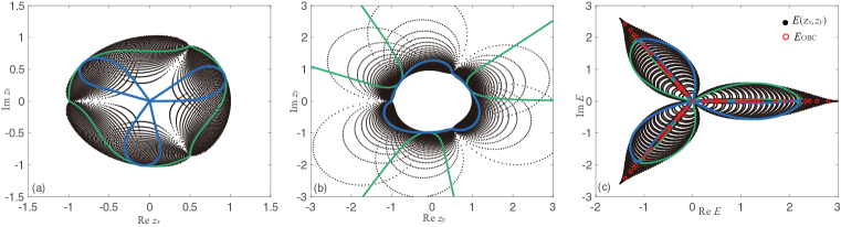
Figure S7: (a,b) Closed paths from the unconstrained GBZ from Eq. S42 to S44 that result in nontrivial spectral winding, in contradiction to the known fact that OBC spectra should not enclose any nonzero area (nontrivial winding). The unconstrained GBZ $z_{x}$ (a) and $z_{y}$ (b) of $H_{\text{2D,III}}$ with $t_{1}=t_{2}=t_{3}=1$ are plotted in black for $k_{1},k_{2}$ ranging over all values in steps of $\pi/100$, with illustrative green and blue closed paths enclosing nonzero area given by $k_{1}=(-\pi/3,\pi/3),k_{2}=\pi/6$ and $k_{2}=(-\pi/3,\pi/3),k_{1}=\pi/6$ respectively. (c) The corresponding spectrum (Eq. S45) from the unconstrained GBZ (black) and the corresponding green and blue spectral loops that enclose non-vanishing areas, which they are not supposed to do. In particular, they do not agree with the correct, numerically obtained OBC spectrum (red), which lies on a subset of $E(z_{x},z_{y})$ points, but which does not exhibit any nontrivial winding.

Since it is knownOkuma et al. (2020); Zhang et al. (2020) that OBC spectra should never possess nonzero spectral winding, which presupposes incomplete NHSE equilibration, the above results Eqs. S44 and S45 cannot possibly give the correct OBC spectrum of $H_{\text{2D, III}}$. Indeed, this is shown in the lack of agreement between the numerically obtained $E_{\text{OBC}}$ spectrum and the (currently unconstrained) GBZ spectrum $E(z_{x},z_{y})$ in Fig. S7. Yet, the above results can be rigorously traced to satisfy all the relations pertaining to the real-space hoppings, and cannot be incorrect. In detail, $z_{x}$ $z_{y}$ are not even proportional to a single phase factor , but $z_{x}=z_{x}(k_{1},k_{2})$,$z_{y}=z_{y}(k_{1},k_{2})$ which 2 phases are twisted with each other. While consider the $x$-direction boundaries, we have $z_{x}(z_{y},k_{1})=z_{x}(z_{y},k’_{1})$ for same $z_{y}$, it’s possible that we can not found the same $z_{y}$ for different $k_{1},k’_{1}$ due to twisted momentum, which indicates that this is not belong to effective BZ. Hence the natural conclusion is that the correct GBZ must be a subset of the GBZ, as currently defined by Eqs. S42 to S44 with the range of $k_{1},k_{2}$ prescribed above. In the below, we shall carefully derive the constraints that extracts the subset of $k_{1},k_{2}$ that generates the correct GBZ for this model; at the end of this supplement, we shall generalize this correct GBZ construction to arbitrary non-Hermitian lattice models.

S3.2 Detailed analysis of constraints leading to dimensional reduction

Here, we elaborate on the possible constraints that can make the energy spectrum (Eq. S45) exhibit zero winding. Since the unconstrained GBZ is a 2D torus that is spanned by 2 homotopy generators, a sure way to remove all possible nonzero spectral windings is to remove the homotopy generator/s that lead to particular nontrivial spectral winding paths. In principle, there can be many ways to remove a homotopy generator, since a combination of generators form another generator. However, for our model $H_{\text{2D,III}}$, it turns out that the requisite constraints can simply take the linear form of $k_{1}=\gamma k_{2}$, with $\gamma$ taking particular values that we shall elaborate on. (Note that we cannot possibly remove both homotopy generators, since there will be no GBZ left then.)

S3.2.1 Analysis of different possible parametrizations

We now justify why it suffices to consider $k_{1}=\gamma k_{2}$, such that the energy takes the 1-parameter form $\bar{E}(k_{2})$ (or equivalently $\bar{E}(k_{1})$), with an slight abuse of notation. First, we establish the range and offset of $k_{1},k_{2}$. given that $z_{1},z_{2}$ (Eqs. S42,S43) satisfy periodicity conditions $z_{1}(k_{1})=z_{1}(k_{1}+2m^{\prime}\pi/(\alpha+\beta))$, $z_{2}(k_{2})=z_{2}(k_{2}+2n^{\prime}\pi/(a+b))$ with integer $n^{\prime},m^{\prime}$ ($n^{\prime},m^{\prime}\in\mathbb{Z}$). We can hence write down a valid linear reparametrization as $k_{1}=\gamma k_{2}+{2n^{\prime}\pi\gamma}/{(a+b)}+{2m^{\prime}\pi}/{(\alpha+\beta)}$ with integer $n^{\prime},m^{\prime}$, such that the energy Eq.(S45) is transformed into $\bar{E}^{\prime}$ as given by

$$\begin{split}&\bar{E}^{\prime}=E(z_{x},z_{y})\Big{|}_{k_{1}=\gamma k_{2}+\frac{2n^{\prime}\pi\gamma}{a+b}+\frac{2m^{\prime}\pi}{\alpha+\beta}}=E\left(z_{1}(k_{1}),z_{2}(k_{2})\right)\Big{|}_{k_{1}=\gamma k_{2}+\frac{2n^{\prime}\pi\gamma}{a+b}+\frac{2m^{\prime}\pi}{\alpha+\beta}}\\ &\quad=E(z_{1}(\gamma k_{2}+2n^{\prime}\pi\gamma/(a+b)),z_{2}(k_{2}))\\ &\quad=\bar{E}\left(k_{2}+\frac{2n^{\prime}\pi}{a+b}\right)\ ,\end{split}$$ (S47)

such as $E^{\prime}\in\{E(k_{2})\}$. Since this hence just a translation of a single coordinate, we can hence just consider constraints of the form $k_{1}=\gamma k_{2}$ without any constant offset. With that,

$$\bar{E}(k_{2})=E(z_{x},z_{y})\Big{|}_{k_{1}=\gamma k_{2}}=E\left(z_{1}(k_{1}),z_{2}(k_{2})\right)\Big{|}_{k_{1}=\gamma k_{2}}=E(z_{1}(\gamma k_{2}),z_{2}(k_{2}))\ .$$ (S48)

Next, we shall show that there exists $3$ possible values of $\gamma$ that guarantee zero spectral winding number while keeping $z_{x},z_{y}$ periodic, namely $\gamma=b/\beta,\ a/\alpha,\ (a+b)/(\alpha+\beta)$. Below are the detailed justifications for the possible choices of $\gamma$ (we call them $\gamma_{1},\gamma_{2}$ and $\gamma_{3}$):

• The case with $k_{1}=\gamma_{1}k_{2}$, $\gamma_{1}=b/\beta$: Here $z_{x},z_{y}$ (S44) and energy (S45) with $k_{1}=bk,k_{2}=\beta k$ are given by

  $$\begin{split}&z_{x,1}^{\alpha+\beta}=\left.z_{x}^{\alpha+\beta}\right|_{k_{1}=\gamma_{1}k_{2}}=\frac{t_{2}\sin((a+b)\beta k)}{t_{1}\sin((\alpha b-a\beta)k)}\text{e}^{i(\alpha b+\beta b)k}\ ,\\ &\left.z_{y,1}^{a+b}=z_{y}^{a+b}\right|_{k_{1}=\gamma_{1}k_{2}}=\frac{t_{3}\sin(\beta bk)\sin((\alpha b-a\beta)k)}{t_{2}\sin(a\beta k)\sin((\alpha b+\beta b)k)}\ ,\end{split}$$ (S49)

  $$\begin{split}\bar{E}_{1}(k)&=\left.E(z_{x},z_{y})\right|_{k_{1}=\gamma_{1}k_{2}=bk}\ ,\\ &=t_{1}^{\frac{\beta}{\alpha+\beta}}t_{2}^{\frac{\alpha b-\beta a}{(\alpha+\beta)(a+b)}}t_{3}^{\frac{a}{a+b}}\text{e}^{\frac{i2\pi av}{a+b}+\frac{2\pi\alpha v^{\prime}}{\alpha+\beta}}\left(\frac{\sin(\alpha b+\beta b)k}{\sin\alpha bk}\right)^{\frac{b}{a+b}}\\ &\qquad\times\left(\frac{\sin(a\beta+\beta b)k}{\sin a\beta k}\right)^{\frac{\alpha}{\alpha+\beta}}\left(\frac{\sin\beta bk}{\sin\alpha bk}\right)^{-\frac{\beta}{\alpha+\beta}}\left(\frac{\sin(a+b)\beta k}{\sin a\beta k}-\frac{\sin(\alpha b+\beta b)k}{\sin\alpha bk}\right)^{\frac{\beta a-\alpha b}{(\alpha+\beta)(a+b)}}\ ,\\ \end{split}$$ (S50)

  where $v=1,2,..,a+b$ , $v^{\prime}=1,2,..,\alpha+\beta$. The range of $k$ has to be dependent on the ratio between $\alpha/\beta$ and $a/b$ as follows:

  • $\alpha/\beta>a/b$: $k$ can take values in $\left(-\frac{\pi}{(\alpha+\beta)b},\frac{\pi}{(\alpha+\beta)b}\right]$. Both $z_{x,1}$ and $z_{y,1}$ are connected end to end with ‘momentum’ $k$, and the path of $z_{x,1}$ in the complex plane forms a closed loop. Hence, the results of $z_{x,1},z_{y,1}$ (Eq.(S49)) are legitimate, and zero winding in the energy $\bar{E}_{1}$ (Eq.(S50)) is respected.

  • $\alpha/\beta=a/b$: $k$ can take values in $\left(-\frac{\pi}{(a+b)\beta},\frac{\pi}{(a+b)\beta}\right]$. And $z_{x,1}^{\alpha+\beta}\rightarrow\infty$,  $z_{y,1}^{a+b}\rightarrow 0$, but the path of $z_{x,1}^{\alpha+\beta}z_{y,1}^{a+b}=\frac{\sin(\beta bk)}{\sin(a\beta k)}\text{e}^{i(a+b)\beta k}$ in the complex plane forms a closed loop with ‘momentum’ $k$. Hence, the results of $z_{x,1},z_{y,1}$ Eq.(S49) are legitimate, and zero winding in the energy $\bar{E}_{1}$ Eq.(S50) is respected.

  • $\alpha/\beta<a/b$: $k$ can take values in $\left(-\frac{\pi}{(a+b)\beta},\frac{\pi}{(a+b)\beta}\right]$. None of $z_{x,1}^{\alpha+\beta}$, $z_{y,1}^{a+b}$, $z_{x,1}^{\alpha+\beta}z_{y,1}^{a+b}$ can form closed loop parametrized by ‘momentum’ $k$. The results of $z_{x,1},z_{y,1}$ and the zero winding requirement of the energy $\bar{E}_{1}$ Eq.(S50) are inconsistent. It is worth noting that when $z^{\alpha+\beta}_{1}=z_{2}^{a+b}$ in Eq.(S44), the $z_{x}^{\alpha+\beta}\rightarrow\infty,z_{y}^{a+b}\rightarrow 0$ which can ignore the end-to-end condition. And in this case, the energy $\bar{E}=0$.

• The case with $k_{1}=\gamma_{2}k_{2}$, $\gamma_{2}=a/\alpha$: $z_{x},z_{y}$ (S44) and the energy (S45) with $k_{1}=ak^{\prime},k_{2}=\alpha k^{\prime}$ are given by

  $$\begin{split}&z_{x,2}^{\alpha+\beta}=\left.z_{x}^{\alpha+\beta}\right|_{k_{1}=\gamma_{2}k_{2}}=\frac{t_{2}\sin(\beta ak^{\prime})\sin((\alpha a+\alpha b)k^{\prime})}{t_{1}\sin(a\alpha k^{\prime})\sin((\alpha b-\beta a)k^{\prime})}\ ,\\ &\left.z_{y,2}^{a+b}=z_{y}^{a+b}\right|_{k_{1}=\gamma_{2}k_{2}}=\frac{t_{3}\sin((\alpha b-a\beta)k^{\prime}))}{t_{2}\sin((\alpha a+a\beta)k^{\prime})}\text{e}^{i(\alpha a+\alpha b)k^{\prime}}\ ,\end{split}$$ (S51)

  $$\begin{split}\bar{E}_{2}(k^{\prime})&=\left.E(z_{x},z_{y})\right|_{k_{1}=\gamma_{2}k_{2}=ak^{\prime}}\ ,\\ &=t_{1}^{\frac{\beta}{\alpha+\beta}}t_{2}^{\frac{\alpha b-\beta a}{(\alpha+\beta)(a+b)}}t_{3}^{\frac{a}{a+b}}\text{e}^{\frac{i2\pi av}{a+b}+\frac{2\pi\alpha v^{\prime}}{\alpha+\beta}}\left(\frac{\sin(\alpha a+\beta a)k^{\prime}}{\sin\alpha ak^{\prime}}\right)^{\frac{b}{a+b}}\\ &\qquad\times\left(\frac{\sin(a\alpha+\alpha b)k^{\prime}}{\sin a\alpha k^{\prime}}\right)^{\frac{\alpha}{\alpha+\beta}}\left(\frac{\sin\beta ak^{\prime}}{\sin\alpha ak^{\prime}}\right)^{-\frac{\beta}{\alpha+\beta}}\left(\frac{\sin(\alpha b-a\beta)k^{\prime}}{\sin a\alpha k^{\prime}}\right)^{\frac{\beta a-\alpha b}{(\alpha+\beta)(a+b)}}\ ,\\ \end{split}$$ (S52)

  where $v=1,2,..,a+b$ , $v^{\prime}=1,2,..,\alpha+\beta$. The range of $k^{\prime}$ similarly has to depend on the ratio between $\alpha/\beta$ and $a/b$:

  • $\alpha/\beta>a/b$, $k^{\prime}$ can take values in $\left(-\frac{\pi}{(a+b)\alpha},\frac{\pi}{(a+b)\alpha}\right]$. Both $z_{x,2}$ and $z_{y,2}$ are connected end to end with ‘momentum’ $k$, and the path of $z_{y,2}$ in complex plane forms a closed loop. Hence, the results of $z_{x,2},z_{y,2}$ (Eq.(S51)) are legitimate, and zero winding in the energy $\bar{E}_{2}$ Eq.(S52) is repected.

  • $\alpha/\beta=a/b$, $k^{\prime}$ can take values in $\left(-\frac{\pi}{(a+b)\alpha},\frac{\pi}{(a+b)\alpha}\right]$. And $z_{x,2}^{\alpha+\beta}\rightarrow\infty$,  $z_{y,2}^{a+b}\rightarrow 0$, but the path of $z_{x,2}^{\alpha+\beta}z_{y,2}^{a+b}=\frac{\sin(\alpha bk^{\prime})}{\sin(\alpha ak^{\prime})}\text{e}^{i(a+b)\alpha k^{\prime}}$ in the complex plane forms a closed loop with ‘momentum’ $k$. Hence, the results of $z_{x,2},z_{y,2}$ Eq.(S51) are legitimate, and zero winding in the energy $\bar{E}_{2}$ Eq.(S52) is repected.

  • $\alpha/\beta<a/b$, $k^{\prime}$ can take values in $\left(-\frac{\pi}{(\alpha+\beta)a},\frac{\pi}{(\alpha+\beta)a}\right]$. None of $z_{x,2}^{\alpha+\beta}$, $z_{y,2}^{a+b}$, $z_{x,2}^{\alpha+\beta}z_{y,2}^{a+b}$ can form closed loop parametrized by ‘momentum’ $k^{\prime}$. The results of $z_{x,2},z_{y,2}$ and the zero winding requirement of the energyy $\bar{E}_{2}$ Eq.(S52) seem unreasonable. It is worth noting that when $z^{\alpha+\beta}_{1}=z_{2}^{a+b}$ in Eq.(S44), the $z_{x}^{\alpha+\beta}\rightarrow\infty,z_{y}^{a+b}\rightarrow 0$ which can ignore the end-to-end condition. And in this case, the energy $\bar{E}=0$.

• The case with $k_{1}=\gamma_{3}k_{2}$, $\gamma_{3}=(a+b)/(\alpha+\beta)$: $z_{x},z_{y}$ (S44) and energy (S45) with $k_{1}=(a+b)k^{\prime\prime},k_{2}=(\alpha+\beta)k^{\prime\prime}$ take the forms

  $$\begin{split}&z_{x,3}^{\alpha+\beta}=\left.z_{x}^{\alpha+\beta}\right|_{k_{1}=\gamma_{3}k_{2}}=\frac{t_{2}\sin(\beta(a+b)k^{\prime\prime})}{t_{1}\sin(\alpha b-\beta a)k^{\prime\prime})}\text{e}^{ib(\alpha+\beta)k^{\prime\prime}}\ ,\\  &\left. z_{y,3}^{a+b}=z_{y}^{a+b}\right|_{k_{1}=\gamma_{3}k_{2}}=\frac{t_{3}\sin(\alpha b-\beta a)k^{\prime\prime})}{t_{2}\sin(a(\alpha+\beta)k^{\prime\prime})}\text{e}^{i\alpha(a+b)k^{\prime\prime}}\ , \end{split}$$ (S53)

  $$\begin{split}\bar{E}_{3}(k^{\prime\prime})&=\left.E(z_{x},z_{y})\right|_{k_{1}=\gamma_{3}k_{2}=(a+b)k^{\prime\prime}}\ ,\\  &=t_{1}^{\frac{\beta}{\alpha+\beta}}t_{2}^{\frac{\alpha b-\beta a}{(\alpha+\beta)(a+b)}}t_{3}^{\frac{a}{a+b}}\text{e}^{\frac{i3\pi av}{a+b}+\frac{3\pi\alpha v^{\prime}}{\alpha+\beta}}\left(\frac{\sin(\alpha+\beta)(a+b)k^{\prime\prime}}{\sin\alpha(a+b)k^{\prime\prime}}\right)^{\frac{b}{a+b}}\left(\frac{\sin(a+b)(\alpha+\beta)k^{\prime\prime}}{\sin a(\alpha+\beta)k^{\prime\prime}}\right)^{\frac{\alpha}{\alpha+\beta}}\\ &\qquad\times\left(\frac{\sin\beta(a+b)k^{\prime\prime}}{\sin\alpha(a+b)k^{\prime\prime}}\right)^{-\frac{\beta}{\alpha+\beta}}\left(\frac{\sin b(\alpha+\beta)k^{\prime\prime}}{\sin a(\alpha+\beta)k^{\prime\prime}}-\frac{\sin\beta(a+b)k^{\prime\prime}}{\sin\alpha(a+b)k^{\prime\prime}}\right)^{\frac{\beta a-\alpha b}{(\alpha+\beta)(a+b)}}\ ,\\ \end{split}$$ (S54)

  where $v=1,2,..,a+b$ , $v^{\prime}=1,2,..,\alpha+\beta$. Here, the range of $k^{\prime\prime}$ is always $\left(-\frac{\pi}{(\alpha+\beta)(a+b)},\frac{\pi}{(\alpha+\beta)(a+b)}\right]$.

  • $\alpha/\beta\neq a/b$: none of $z_{x,3}^{\alpha+\beta}$, $z_{y,3}^{\alpha+\beta}$, $z_{x,3}^{\alpha+\beta}z_{y,3}^{\alpha+\beta}$ can form closed loop parametrized by momentum $k^{\prime\prime}$. Hence the results of $z_{x,3},z_{y,3}$ (Eq.(S53)) are inadmissible, since they are inconsistent with the zero winding requirement of the energy $E_{3}$ Eq.(S54).

  • $\alpha/\beta=a/b$: this case is equivalent to the case $k_{1}=\gamma_{1}k_{2}$ or $k_{1}=\gamma_{2}k_{2}$ with $\alpha/\beta=a/b$.

  Hence, the case with $k_{1}=\gamma_{3}k_{2}$, $\gamma_{3}=(a+b)/(\alpha+\beta)$ can incorporate the cases with $k_{1}=\gamma_{1,2}k_{2}$ ($\gamma_{1}=b/\beta,\gamma_{2}=a/\alpha$).

S3.2.2 Summary

Table 1: Brief summary of admissible GBZs for our type III model (Eq. S40)

(Shaded boxes represent valid contributing GBZ sectors) $k_{1}=\gamma_{1}k_{2}$ $(\gamma_{1}=\frac{b}{\beta})$ $k_{1}=\gamma_{2}k_{2}$ $(\gamma_{2}=\frac{a}{\alpha})$ $k_{1}=\gamma_{3}k_{2}$$(\gamma_{3}=\frac{a+b}{\alpha+\beta})$ $z_{x(y),1}=\left.z_{x(y)}\right|_{k_{1}=\gamma_{1}k_{2}}$ $z_{x(y),2}=\left.z_{x(y)}\right|_{k_{1}=\gamma_{2}k_{2}}$ $z_{x(y),3}=\left.z_{x(y)}\right|_{k_{1}=\gamma_{3}k_{2}}$ ${\alpha/\beta>a/b}$ $z_{x,1}$: closed loop $z_{x,2}$: real $z_{x,3}$, $z_{y,3}$, $z_{x,3}^{\alpha+\beta}z_{y,3}^{\alpha+\beta}$: open loop $z_{y,1}$: real $z_{y,2}$: closed loop Hence GBZ=$\text{GBZ}_{1}\cup\text{GBZ}_{2}$ (with $\text{GBZ}_{1}=\left\{z_{x,1},z_{y,1}\right\}$, $\text{GBZ}_{2}=\left\{z_{x,2},z_{y,2}\right\}$) ${\alpha/\beta=a/b}$ $z_{i,1}=z_{i,2}=z_{i,3}$ ($i=x,y$) and $z_{x,1}\rightarrow\infty,\ z_{y,1}\rightarrow 0$ $z^{\alpha+\beta}_{x,1}z^{a+b}_{y,1}$: closed loop Hence $\text{GBZ}=\left\{z^{\alpha+\beta}_{x,1}z^{a+b}_{y,1}\right\}$ ${\alpha/\beta<a/b}$ $z_{x,j}\rightarrow\infty,\ z_{y,j}\rightarrow 0$  ($j=1,2,3$) $\bar{E}=0$

To summarize, the (correct) constrained GBZ of $H_{\text{2D, III}}$ of Eq.(S40) is not 2D, but is made up of one or more disconnected 1D loops as described above, depending on the hopping lengths $\alpha,\beta,a,b$. We call the effective Hamiltonian constrained to this reduced GBZ $H_{\text{2D-red}}$:

• When $\alpha/\beta>a/b$, the GBZ and spectrum consists of the union of the two sectors

  $$\begin{split}&\ \quad\qquad\qquad\text{GBZ}=\text{GBZ}_{1}\cup\text{GBZ}_{2},\\ &\text{GBZ}_{1}=\left\{z_{x,1},z_{y,1}\left|k\in\left(-\frac{\pi}{(\alpha+\beta)b},\frac{\pi}{(\alpha+\beta)b}\right]\right.\right\},\\ &\text{GBZ}_{2}=\left\{z_{x,2},z_{y,2}\left|k^{\prime}\in\left(-\frac{\pi}{(a+b)\alpha},\frac{\pi}{(a+b)\alpha}\right]\right.\right\}, \end{split}$$ (S55)

  $$\begin{split}\{\bar{E}\}=\{\bar{E}_{1}\}\cup\{\bar{E}_{2}\},\\  \end{split}$$ (S56)

  where the forms of $z_{x(y),1(2)}$ can be found in Eq.(S49,S51) and that of $E_{1,2}$ can be found in Eq.(S50,S52). Unlike with the unconstrained GBZ, they agree excellently with numerics, as shown in the example in FIG. S8. In other words, the effective surrogate OBC Hamiltonian of the case $\alpha/\beta>a/b$ takes the form

  $$\bar{H}_{\text{2D-red}}=\bar{H}_{\text{2D,III}}=\bar{H}_{1}\oplus\bar{H}_{2}\ ,$$ (S57)

  where $\bar{H}_{1}$ and $\bar{H}_{2}$ are the Hamiltonian operators with corresponding spectra $\bar{E}_{1}$ and $\bar{E}_{2}$ (Eqs. S50 and S52).

  

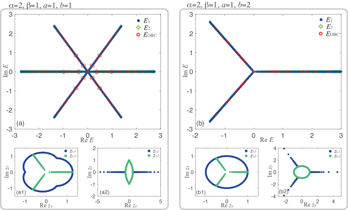
  Figure S8: The constrained GBZs and corresponding spectra $\bar{E}$ of two illustrative cases of $H_{\text{2D, III}}$ with hopping lengths $\alpha/\beta>a/b$, as indicated on top of the panels. Top) Coincident spectral contributions $\bar{E}_{1},\bar{E}_{2}$ from 1D GBZ sectors $1$ and $2$ of these 2D lattices, as defined in Eq.(S50,S52). They agree well with the numerical $E_{\text{OBC}}$ which is here computed with $10\times 10$ lattice sites, with density of states comparison presented later. Bottom) 1D GBZs $z_{x},z_{y}$ Eq.(S49,S51) for sectors $1$ and $2$, which traces loops or flattened loops in the complex plane, consistent with the conclusions from Table. 1. The two GBZ sectors may look totally different from each other, but they combine to describe the system as a coherent whole. Parameters are $t_{1}=t_{1}=t_{3}=1$ and the GBZs are plotted with $k,k^{\prime}$ points at intervals of $\pi/300$.

• When $\alpha/\beta=a/b$, the GBZ and spectrum are given by

  $$\begin{split}\text{GBZ}=\left\{z_{x,1}^{\alpha+\beta}z_{y,1}^{a+b}=\frac{\sin(\beta bk)}{\sin(a\beta k)}\text{e}^{i(a\beta+\beta b)k}\left|k\in\left(-\frac{\pi}{(a+b)\beta},\frac{\pi}{(a+b)\beta}\right]\right.\right\}, \end{split}$$ (S58)

  $$\begin{split}\bar{E}(k)=t_{1}^{\frac{b}{a+b}}t_{3}^{\frac{a}{a+b}}\left(\frac{\sin(a+b)\beta k}{\sin a\beta k}\right)\left(\frac{\sin\beta bk}{\sin a\beta k}\right)^{-\frac{b}{a+b}}\text{e}^{\frac{2i\pi av^{\prime}}{a+b}}\ ,\\  \end{split}$$ (S59)

  with excellent numerical agreement as shown in FIG. S9.

  

  Figure S9: The constrained GBZs and corresponding spectra $\bar{E}$ of $H_{\text{2D, III}}$ of two illustrative cases with hopping lengths $\alpha/\beta=a/b$ as indicated in the panels. Top) Spectrum according to the GBZ (Eq.(S59)), which agree well with the numerical $E_{\text{OBC}}$ spectrum which is here computed with $20\times 20$ lattice sites. Bottom) Corresponding constrained 1D GBZs $z_{x},z_{y}$ (Eq. (S58)) of these 2D lattices, with cusps that are not present in the GBZs of 1D non-Hermitian lattices. Parameters are $t_{1}=t_{1}=t_{3}=1$ and the GBZ is plotted with $k$ points at intervals of $\pi/600$.

• When $\alpha/\beta<a/b$, the energy is always zero and $z_{x}^{\alpha+\beta}\rightarrow\infty$,  $z_{y}^{a+b}\rightarrow 0$, which means that the eigenstates always corner-localize, as illustrated in FIG. S10. This is due to non-Bloch collapse, since hoppings $t_{1}$ and $t_{3}$ do not contain any net component that in the inverse direction of hopping $t_{2}$.

Figure S10: (Top) Identically zero energies for the case of $\alpha\beta<a/b$ of the type III system Eq.(S40) ($\bar{E}=0$ are from theoretical analysis , $E_{\text{OBC}}=0$ are numerical OBC eigenvalues). (Bottom) corresponding corner-localized distribution of eigenstates. The system parameters are $t_{1}=t_{1}=t_{3}=1$, with $\alpha,\beta,a,b$ indicated in the figures.

S3.2.3 Number of OBC spectral branches for type III hopping lattices

To find the number of OBC spectral branches for $H_{\text{2D,III}}$ satisfies the symmetry

$$\begin{split}&U_{v,v^{\prime}}^{-1}H_{\text{2D,III}}U_{v,v^{\prime}}=\exp\left(i\frac{2\alpha\pi}{\alpha+\beta}v+i\frac{2a\pi}{a+b}v^{\prime}\right)H_{\text{2D,III}}\ ,\\ &U_{v,v^{\prime}}=\exp\left(i\frac{2m\pi}{\alpha+\beta}v+i\frac{2n\pi}{a+b}v^{\prime}\right)|m,n\rangle\langle m,n|\ ,\end{split}$$ (S60)

with integer indices $v,v^{\prime}$ ($v=1,2,..,\alpha+\beta,\,v^{\prime}=1,2,...,a+b$), where $|m,n\rangle$ are real space basis orbitals. $U_{v,v^{\prime}}$ is a unitary operator which satisfies $U_{v,v^{\prime}}U_{v,v^{\prime}}^{\dagger}=\text{I}$ , (‘I’ represents the unit operator). Assuming that the wave function $|\Psi^{n}\rangle$ is an eigenstate of the model Eq.(S40) with eigenvalue $E_{n}$, the other eigenstates $U_{v,v^{\prime}}|\Psi^{n}\rangle$ can be found via symmetry Eq.(S60) with eigenvalue $\exp\left(i\frac{2\alpha\pi}{\alpha+\beta}v+i\frac{2a\pi}{a+b}v^{\prime}\right)E_{n}$, that is,

$$\begin{split}H_{\text{2D,III}}|\Psi^{n}\rangle&=E_{n}|\Psi^{n}\rangle\ ,\\ \exp\left(i\frac{2\alpha\pi}{\alpha+\beta}v+i\frac{2a\pi}{a+b}v^{\prime}\right)H_{\text{2D,III}}|\Psi^{n}\rangle&=\exp\left(i\frac{2\alpha\pi}{\alpha+\beta}v+i\frac{2a\pi}{a+b}v^{\prime}\right)E_{n}|\Psi^{n}\rangle\ ,\\ U_{v,v^{\prime}}^{-1}H_{\text{2D,III}}U_{v,v^{\prime}}|\Psi^{n}\rangle&=\exp\left(i\frac{2\alpha\pi}{\alpha+\beta}v+i\frac{2a\pi}{a+b}v^{\prime}\right)E_{n}|\Psi^{n}\rangle\ ,\\ H_{\text{2D,III}}U_{v,v^{\prime}}|\Psi^{n}\rangle&=\exp\left(i\frac{2\alpha\pi}{\alpha+\beta}v+i\frac{2a\pi}{a+b}v^{\prime}\right)E_{n}U_{v,v^{\prime}}|\Psi^{n}\rangle\ .\\ \end{split}$$ (S61)

Hence we see that the energy spectrum of $H_{\text{2D,III}}$ is parametrized by a 1-parameter family of states, with indices $v,v^{\prime}$ taking $\alpha+\beta$,$a+b$ possible values. As such, there are

$$\text{LCM}\left[\displaystyle\frac{a+b}{\text{GCD}(a+b,a)},\frac{\alpha+\beta}{\text{GCD}(\alpha+\beta,\alpha)}\right]\ ,$$ (S62)

OBC spectral branches for type III lattices.

S3.2.4 Flowchart of our approach

All in all, the procedure of obtaining the effective BZ and spectrum is illustrated in the following flowchart for generic 2D models. Higher-dimensional models can be dealt with analogously, and will be discussed later.

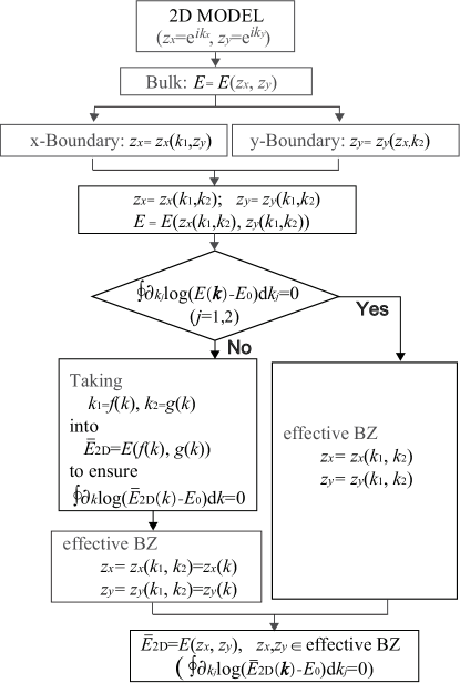
Figure S11: Flowchart of our approach for generic 2D models. Starting with the original model which can be expressed as $E(z_{x},z_{y})$ by identifying $z_{x}=e^{ik_{x}}$, $z_{y}=e^{ik_{y}}$, we find how $z_{x},z_{y}$ depend on $k_{1},k_{2}$ by implementing x and y-OBCs separately. If the resulting spectrum does not contain nontrivial spectral winding, the effective BZ is still 2D and we are done. If not, we find 1D parametrizations $k$ of a submanifold of the $(k_{1},k_{2})$ torus such that the spectral windings are trivial. The effective 1D BZ comprises all such 1D paths.

S3.3 Density of states in the dimensionally-reduced effective system

In the subsection above, we have shown that in order for the GBZ spectrum of $H_{\text{2D,III}}$ (Eq. S40) to exhibit nonzero winding for any closed path, there is a need to constrain the valid GBZ to a 1D subspace of the original naively obtained 2D GBZ. Here, we show that the numerically obtained OBC spectrum indeed correspond to equally spaced states in the 1D constrained BZ, just like how the momentum eigenstates are distributed in 1D BZ corresponding to a physically 1D system.

To verify that the spectrum of $H_{\text{2D-red}}$ indeed comprises equally-spaced “momentum” eigenstates, we examine the density of states (DOS) of the OBC spectrum. The DOS is given by

$$\begin{split}\rho(E)=\frac{1}{N}\frac{\delta n}{\delta E}\ ,\end{split}$$ (S63)

which means that there are $\delta n$ eigenstates in the energy range $[E,E+\delta E)$ and normalization constant $N$ is equal to the length of the energy to be measured. What we would like to check is the quantity $\sigma(k)$, which is the DOS in momentum space. That is, the momentum range $[k_{i},k_{i}+\delta k_{i})$ $(i=1,2)$ which corresponds to energy range $[E,E+\delta E)$ need to be considered, where $i=1,2$ refers to the possible sectors for the GBZs. If the states are indeed uniformly labeled by momentum, $\sigma_{i}(k)\propto\rho_{i}(E){\delta E_{i}}/{\delta k}$ should be uniform in each sector $i$, and $\sigma(k)=\sum_{i}\sigma_{i}(k)$ should only be proportional to the number of sectors corresponding to a particular value of $k$. For OBC states predicted by the GBZ sector energies $\bar{E}_{i}$, we have

$$\begin{split}\sigma(k)&=\sum_{i}\sigma_{i}(k)=\frac{2\pi}{\mathcal{N}}\sum_{i}\frac{\delta n_{i}(k)}{\delta E_{i}(k)}\frac{\delta E_{i}(k)}{\delta k}=\sum_{i}\delta n_{i}(k)\ ,\\ \end{split}$$ (S64)

with $\delta k=2\pi/\mathcal{N}$. For each energy interval $\delta E(k)=\bar{E}_{i}(k+\delta k)-\bar{E}_{i}(k)$, one can obtain the number $\delta n(k)$ of occupied states within the interval. With the knowledge of the dependence between $\bar{E}_{i}$ of the GBZ and momentum $k$ , it’s easy to get the DOS in momentum space $\sigma(k)$. This is shown in FIG.S12(a,b) for two illustrative sets of parameters.

S3.3.1 Model with the GBZ sectors possessing the same energies

For definiteness, we first consider $H_{\text{2D,III}}$ Eq.(S40) with $\alpha=2,\beta=1,a=1,b=2$, such that the energy takes the form

$$\begin{split}E(z_{x},z_{y})=t_{1}z_{x}^{2}z_{y}+t_{2}z_{x}^{-1}z_{y}+t_{3}z_{x}^{-1}z_{y}^{-2},\end{split}$$ (S65)

where each of $z_{x},z_{y}$ belongs to the 1D GBZ sectors $\text{GBZ}_{1}$ and $\text{GBZ}_{2}$, which from Sec. S3.2 Eq.(S55, S56) simplify to

$$\begin{split}\text{GBZ}_{1}&=\left\{\left.z_{x,1}^{3}=\frac{t_{2}}{t_{1}}\text{e}^{ik},z_{y,1}^{3}=\frac{t_{3}}{t_{2}}\frac{1}{2\cos\left(k/3\right)-1}\right|k\in[-\pi,\pi)\right\}\ ,\\ \text{GBZ}_{2}=&\left\{\left.z_{x,2}^{3}=\frac{t_{2}}{t_{1}}\left(2\cos\left(k^{\prime}/3\right)-1\right),z_{y,2}^{3}=\frac{t_{3}}{t_{2}}\text{e}^{-ik^{\prime}},\right|k^{\prime}\in[-\pi,\pi)\right\}\ ,\\ &\qquad\qquad\text{GBZ}=\text{GBZ}_{1}\cup\text{GBZ}_{2}\ .\end{split}$$ (S66)

In other words, the set of GBZ eigenstates consists of eigenstates from both GBZ sectors. The OBC eigenenergies are approximated by GBZ energies, which are given either by $E(z_{x,1},z_{y,1})=\bar{E}_{1}(k)$ or $E(z_{x,2},z_{y,2})=\bar{E}_{2}(k^{\prime})$, where $k$ and $k^{\prime}$ parametrize their respective GBZs. The GBZ Hamiltonian is hence given by

$$\begin{split}H_{\text{2D-red}}&=\bar{H}_{\text{2D,III}}={H}_{1}\oplus{H}_{2}\ ,\\ \bar{E}_{1}(k)=\bar{E}_{2}(k)&=t_{1}^{1/3}t_{2}^{1/3}t_{3}^{1/3}(2\cos(k/3)+1)^{1/3}(2\cos(2k/3)+1)^{2/3}\text{e}^{2i\pi v/3}\ ,\end{split}$$ (S67)

with $k,k^{\prime}\in(-\pi,\pi]$, $v=1,2,3$, see FIG. S12(a). $\bar{E}_{1}$ and $\bar{E}_{2}$ are the corresponding eigenenergies of $H_{1}$ and $H_{2}$; in this case, after substituting the sector-dependent forms of $z_{x,\nu}$ and $z_{y,\nu}$, they happen to take identical functional forms.

To justify the integrity of this GBZ construction, we first note that the spectral winding number is zero, since Eq.(S67) is obviously real. Also, both the GBZ₁ and GBZ₂ are period in $k,k^{\prime}$. The correctness of Eq.(S66,S67) is demonstrated in FIG. S8(b), which not only shows that the results of the GBZ and GBZ Hamiltonian can be trusted, but also that the relation between OBC energies and momentum $k$ are as expected.

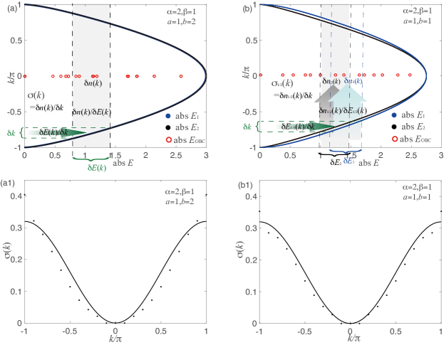
Figure S12: Density of states (DOS) in momentum space. (a,b) The solid curves denote the dependence of effective 1D GBZ sector energies $E_{1},E_{2}$ with momentum $k$ for two possible models Eq.(S41). Numerically, we can obtain $k\approx k+\delta k$ from each $\delta E(k)$ point from $E_{\text{OBC}}$ data (red circles, shown on the central horizontal), and obtain the momentum space DOS $\sigma(k)$.
(a1,b1) The momentum space DOS profile $\sigma(k)$ in our model Eq.(S41), with $\delta k=\pi/8000$. For both models, the DOS (black dots) can be approximately fitted to a sinusoidal curve (black curve). Parameters are $t_{1}=t_{1}=t_{3}=1$, with a OBC lattice of $L^{2}=10^{2}=100$ sites.

S3.3.2 Model with the GBZ sectors possessing different energies

In the above, we considered $H_{\text{2D,III}}$ (Eq.(S40)) with $\alpha=b$ and $\beta=a$, such that the two 1D GBZ sectors correspond to eigenenergies $\bar{E}_{1}$ and $\bar{E}_{2}$ Eq.(S67) with equivalent forms. That, however, is not the case for more generic models. Here, we consider an illustrative model with $\alpha=2$, $\beta=1,a=1,b=1$ with dissimilar GBZ eigenenergies for its two sectors. We first write it in terms of $z_{x},z_{y}$:

$$\begin{split}E(z_{x},z_{y})=t_{1}z_{x}^{2}z_{y}+t_{2}z_{x}^{-1}z_{y}+t_{3}z_{x}^{-1}z_{y}^{-1}\ ,\end{split}$$ (S68)

where each of $z_{x},z_{y}$ belongs to either of the two GBZ sectors

$$\begin{split}\text{GBZ}_{1}&=\left\{\left.z_{x,1}^{3}=\frac{t_{2}}{t_{1}}2\cos(k/3)\text{e}^{ik},z_{y,1}^{3}=\frac{t_{3}}{t_{2}}\frac{1}{2\cos\left(2k/3\right)+1}\right|k\in[-\pi,\pi)\right\}\ ,\\ \text{GBZ}_{2}=&\left\{\left.z_{x,2}^{3}=\frac{t_{2}}{t_{1}}\frac{\sin(3k^{\prime}/4)}{\sin(k^{\prime}/2)},z_{y,2}^{3}=\frac{t_{3}}{t_{2}}\frac{1}{2\cos\left(k/2\right)+1}\text{e}^{-ik^{\prime}},\right|k^{\prime}\in[-\pi,\pi)\right\}\ ,\\ &\qquad\qquad\text{GBZ}=\text{GBZ}_{1}\cup\text{GBZ}_{2}\ ,\end{split}$$ (S69)

as introduced in Sec. S3.2 Eq.(S55, S56). GBZ eigenenergies $\bar{E}$ take the form of either $E(z_{x,1},z_{y,1})=\bar{E}_{1}(k)$ or $E(z_{x,2},z_{y,2})=\bar{E}_{2}(k^{\prime})$, with their GBZ Hamiltonian and explicit eigenenergies

$$\begin{split}&\bar{H}_{\text{2D-red}}=\bar{H}_{\text{2D,III}}=\bar{H}_{1}\oplus\bar{H}_{2},\\ \bar{E}_{1}(k)=\pm t_{1}^{1/3}t_{2}^{1/6}t_{3}^{1/2}&(2\cos(2k/3)+1)^{1/2}(2\cos(k/3))^{2/3}\text{e}^{2i\pi v/3}\ ,\\ \bar{E}_{2}(k^{\prime})=\pm t_{1}^{1/3}t_{2}^{1/6}t_{3}^{1/2}&(2\cos(k^{\prime}/2)+1)^{1/2}(2\cos(k^{\prime}/2))^{2/3}(\sin(k^{\prime}/4))^{2/3}\text{e}^{2i\pi v/3}\ ,\end{split}$$ (S70)

with $k,k^{\prime}\in(-\pi,\pi]$, $v=1,2,3,$ for the model Eq.(S68). As in the previous example, the spectral winding in Eq.(S70) are both zero, and both GBZ₁ and GBZ₂ are periodic. However, here $\bar{E}_{1}(k)$ and $\bar{E}_{2}(k)$ manifestly take different functional forms. As presented in FIG. S8(a), the numerical results demonstrate the correctness of Eq.(S69,S70), with both $\bar{E}_{1}(k)$ and $\bar{E}_{2}(k)$ agreeing with the distribution of numerically obtained $E_{\text{OBC}}$. Note that strictly, the above GBZ results are exact only in the continuum limit ($L\rightarrow\infty$) where the set of momenta $k$ tends towards an equally spaced set of points with $\sim L^{-1}$ separation.

S3.4 Circuit simulation of non-Hermitian lattices

Any electrical circuit network can be represented by a graph whose nodes and edges correspond to the circuit junctions and connecting wires/elements. The circuit behavior is fundamentally described by Kirchhoff’s law. Non-Hermiticity can be introduced in a RLC electrical circuit by means of negative impedance converters with current inversion (INICs)Ningyuan et al. (2015); Lee et al. (2018b); Hofmann et al. (2019); Stegmaier et al. (2021); Liu et al. (2021); Hofmann et al. (2020); Helbig et al. (2020); Ezawa (2019) (Fig. S13(c1)). By means of Kirchhoff’s law, it can be shown that Ningyuan et al. (2015); Lee et al. (2018b); Hofmann et al. (2019); Stegmaier et al. (2021); Imhof et al. (2018); Helbig et al. (2019); Zhang et al. (2019); Helbig et al. (2020); Lee et al. (2020b); Zhang and Franz (2020); Hofmann et al. (2020); Lenggenhager et al. (2021); Liu et al. (2021); Zou et al. (2021); Liu et al. (2020b); Hohmann et al. (2022); Zhang et al. (2023b); Bergholtz et al. (2021); Ezawa (2019) each INIC possess the reduced 2-node Laplacian

$$\begin{split}\left(\begin{array}[]{c}I^{\prime}_{\text{in}}\\ I^{\prime}_{\text{out}}\\ \end{array}\right)=\frac{1}{2i\omega L}\left(\begin{array}[]{cc}1&-1\\ 1&-1\\ \end{array}\right)\left(\begin{array}[]{c}V_{\text{in}}\\ V_{\text{out}}\\ \end{array}\right).\end{split}$$ (S71)

If we further connect an INIC with an inductor of inductance $2L$ in parallel, we obtain

$$\begin{split}\left(\begin{array}[]{c}I_{\text{in}}\\ I_{\text{out}}\\ \end{array}\right)=\frac{1}{i\omega L}\left(\begin{array}[]{cc}1&-1\\ 0&0\\ \end{array}\right)\left(\begin{array}[]{c}V_{\text{in}}\\ V_{\text{out}}\\ \end{array}\right).\end{split}$$ (S72)

for this parallel configuration pair. This INIC-inductor pair is very versatile, and can be used as the building block of arbitrary non-Hermitian circuit Laplacians. In general, circuit Laplacians $J$ are obtained via Kirchhoff rule $\bm{I}=J\bm{V}$ , where $I$ denotes the current input and the voltage $\bm{V}$ measures against ground at each node. As an initial step towards identifying circuits with tight-binding lattice models, we can get $\bm{I}=J\bm{V}$ in compact matrix form (Fig. S13(c))

$$\begin{split}\left(\begin{array}[]{c}I_{1}^{m,n}\\ I_{2}^{m,n}\\ I_{3}^{m,n}\\ I_{4}^{m,n}\\ \end{array}\right)=\left(\begin{array}[]{cccc}-{1}/{(i\omega L_{1})}&0&0&{1}/{(i\omega L_{1})}\\ 0&-{1}/{(i\omega L_{2})}&0&{1}/{(i\omega L_{2})}\\ 0&0&-{1}/{(i\omega L_{3})}&{1}/{(i\omega L_{3})}\\ 0&0&0&i\omega C\end{array}\right)\left(\begin{array}[]{c}V_{m+2,n+1}\\ V_{m-1,n+1}\\ V_{m-1,n-2}\\ V_{m,n}\end{array}\right).\end{split}$$ (S73)

For instance, the circuit in Fig. S13 (c), shown for just one unit cell, is mathematically described by a Laplacian matrix, which in momentum space under PBCs, takes the form

$$\begin{split}&I(\bm{k})=J(\bm{k})V(\bm{k})\ ,\\ J(\bm{k})=\mu+&t_{1}\text{e}^{2ik_{x}+ik_{y}}+t_{2}\text{e}^{-ik_{x}+ik_{y}}+t_{3}\text{e}^{-ik_{x}-2ik_{y}}\ ,\end{split}$$ (S74)

with $t_{j}=-1/i\omega L_{j}$, $j=1,2,3,$ and $\mu=i\omega C-\sum_{j=1,2,3}t_{j}$. This takes the same form as a tight-binding Hamiltonian of the form (FIG. S13(a))

$$\begin{split}&H=\sum_{m,n}t_{1}|m,n\rangle\langle m+2,n+1|+t_{2}|m,n\rangle\langle m-1,n+1+t_{3}|m,n\rangle\langle m-1,n-2|\ ,\end{split}$$ (S75)

with $H=t_{1}\text{e}^{2ik_{x}+ik_{y}}+t_{2}\text{e}^{-ik_{x}+ik_{y}}+t_{3}\text{e}^{-ik_{x}-2ik_{y}}=J(\bm{k})-\mu$ when expressed in momentum space.

Notably, the system is sensitive to the boundary orientation, in that the effective lattice takes different forms under different boundary orientations, as shown in FIG. S13 (b1-b3), which correspond to the type I to III models discussed in this work. They correspond to their respective circuits in FIG. S13 (d1-d3).

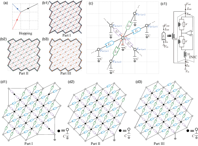
Figure S13: (a) The three hoppings (black,blue,red) that define the model of Eq.(S75). (b1-b3) Different double OBC boundary orientations on this model lattice gives rise to effective models with hoppings that are oriented differently (labeled as Parts I, II and III). (c) To realize this model with an electrical circuit, each asymmetric hopping can be realized with an INIC $L_{i}$, $i=1,2,3$. (c1) gives the internal make-up of an INIC, with the operation amplifier (triangle) giving rise to the hopping asymmetry. (d1-d3) Circuit realizations of the model variations (b1) to (b3).

S4 IV. 2D model with topological zero modes from 1D topological invariant

Here we present a nontrivial implication of the effectively 1D GBZ of our 2D model of the class $H_{\text{2D,III}}$. Since the GBZ construction pertains to not just the spectrum, but represents a complex analytic deformation of the Hamiltonian operator itself (to a so-called surrogate Hamiltonian, see Ref. Lee et al. (2020a)), it means that the OBC properties of such Hamiltonians are also nontrivially modified. In particular, an OBC feature of particular interest is the presence of topological zero modes. Below, we shall see how our model, which is defined in 2D, nevertheless host topological zero modes defined by a 1D topological invariant.

Noting that the GBZ construction is completely determined by the characteristic polynomial (bulk energy dispersion), we can construct a 2-band topological Hamiltonian with a 1D constrained GBZ by writing down a model with exactly the same eigenenergy dispersion as Eq.(S41) up to a constant offset $c$ that gaps the system, i.e.

$$H=\left(\begin{array}[]{cc}0&H_{12}\\ H_{21}&0\\ \end{array}\right),$$ (S76)

with eigenenergies $\mathcal{E}_{1,2}$, which are stipulated to satisfy $\left(\mathcal{E}_{1,2}\right)^{2}=H_{12}H_{21}=E+c=t_{1}z_{x}^{\alpha}z_{y}^{a}+t_{2}z_{x}^{-\beta}z_{y}^{a}+t_{3}z_{x}^{-\beta}z_{y}^{-b}+c$, and

$$\begin{split}H_{12}=\left(E+c\right)/Z&=\left(t_{1}z_{x}^{\alpha}z_{y}^{a}+t_{2}z_{x}^{-\beta}z_{y}^{a}+t_{3}z_{x}^{-\beta}z_{y}^{-b}+c\right)/Z\ ,\\ &\quad\qquad H_{21}=Z\ ,\end{split}$$ (S77)

where we allow $Z$ to assume either of the two forms for illustrative purposes: $Z=z^{a}_{y}$ or $Z=z^{-\beta}_{x}$. $E$ is the energy function of Eq.S41. The gap induced by $c$ does not affect the GBZ solutions since energy degeneracies are not sensitive to a constant offset.

First, for the model Eq.(S40) with OBCs, either along one or both boundary directions, the spectrum of the GBZ hamiltonian must have a net zero winding number, even though the winding number of the off-diagonal term $H_{12}$ is dependent on the $Z$ term.

With $\alpha/\beta>a/b$, its GBZ Hamiltonian takes the form

$$\bar{H}=\bar{H}_{1}\oplus\bar{H}_{2}=\left(\begin{array}[]{cc}0&\bar{H}_{12}\\ \bar{H}_{21}&0\\ \end{array}\right)=\left(\begin{array}[]{cc}0&\bar{H}^{1}_{12}\\ \bar{H}^{1}_{21}&0\\ \end{array}\right)\oplus\left(\begin{array}[]{cc}0&\bar{H}^{2}_{12}\\ \bar{H}^{2}_{21}&0\\ \end{array}\right)\ ,$$ (S78)

$$\bar{H}^{i}_{12}=(\bar{E}_{i}+c)/Z_{i},\quad\bar{H}^{i}_{21}=Z_{i}\ .$$ (S79)

with $\bar{E}_{i}=\bar{H}^{i}_{12}\bar{H}^{i}_{21}$, ($i=1,2$) Eq.(S50,S52). Both $\bar{H}^{i}_{12}$, $i=1,2$ have the same forms of $z_{x,i},z_{y,i}$:

$$\begin{split}&z_{x,1}^{\alpha+\beta}=\frac{t_{2}\sin((a+b)\beta k)}{t_{1}\sin((\alpha b-a\beta)k)}\text{e}^{i(\alpha b+\beta b)k},\quad z_{y,1}^{a+b}=\frac{t_{3}\sin(\beta bk)\sin((\alpha b-a\beta)k)}{t_{2}\sin(a\beta k)\sin((\alpha b+\beta b)k)},\qquad k\in\left[-\frac{\pi}{(\alpha+\beta)b},\frac{\pi}{(\alpha+\beta)b}\right],\\ &z_{x,2}^{\alpha+\beta}=\frac{t_{2}\sin(\beta ak^{\prime})\sin((\alpha a+\alpha b)k^{\prime})}{t_{1}\sin(a\alpha k^{\prime})\sin((\alpha b-\beta a)k^{\prime})}\ ,\ z_{y,2}^{a+b}=\frac{t_{3}\sin((\alpha b-a\beta)k^{\prime}))}{t_{2}\sin((\alpha a+a\beta)k^{\prime})}\text{e}^{i(\alpha a+\alpha b)k^{\prime}},\ k^{\prime}\in\left[-\frac{\pi}{\alpha(a+b)},\frac{\pi}{\alpha(a+b)}\right]\ ,\end{split}$$ (S80)

For each GBZ sector $i$, we have $Z_{i}=z^{a}_{y,i}$ or $Z_{i}=z^{-\beta}_{x,i}$ depending on the choice of illustrative example.

Since we have designed this model such that it harbors nontrivial topological zero modes under double OBCs, from established results Lee and Thomale (2019), both $\bar{H}_{12}$ and $\bar{H}_{21}$ must have nonzero winding about $E=0$ (we shall suppress the GBZ sector label $i$ unless it is explicitly referred to), and these windings sum to zero. For the off-diagonal term $\bar{H}_{12}$, the winding number about $E=0$

$$\begin{split}\omega(\bar{H}_{12})&=\oint\text{d}k\,\partial_{k}\log\bar{H}_{12}=\omega(\bar{H}^{1}_{12})+\omega(\bar{H}^{2}_{12})\neq 0\ ,\\ \end{split}$$ (S81)

is also nonzero. We emphasize that although this nonzero winding criterion for topological modes was originally formulated for a 1D system, we have now used it for the 1D effective GBZ of a physically 2D system. Some examples of cases with topological zero modes for double OBCs but not single OBCs are given in Fig. S14.

However, this model with a single OBC exhibit very different results. If we choose $Z=z^{a}_{y}$, only when the $\bm{x}$ PBC, $\bm{y}$ OBC, the system has topological zero modes, the winding number of $\bar{H}_{12}$ is non-zero on the single OBC GBZ. By contrast, the same system with $\bm{x}$ OBC, $\bm{y}$ PBC has no topological zero modes (Fig. S14). With double OBCs, the 1D GBZ for the double OBCs give rise to zero winding number for $\bar{H}^{1}_{12}$, and nonzero winding number for $\bar{H}^{2}_{12}$, both summing to a nonzero total winding of $\bar{H}_{2}$ from Eq. S78.

If we choose $Z=z^{-\beta}_{x}$ instead, the opposite is the case, the system with $\bm{x}$ OBC, $\bm{y}$ PBC have topological zero modes, the system with $\bm{x}$ PBC, $\bm{y}$ OBC does not have. The winding number of $\bar{H}^{1}_{12}$ is non-zero, the winding number of $\bar{H}^{2}_{12}$ is zero in the GBZ Hamiltonian with double OBC. In an analogous way, the 2D model with double OBC also has topological zero modes which is contributed by $\bar{H}_{1}(k)$ from Eq.S78.

We demonstrate the above arguments for two illustrative cases of $\alpha,\beta,a,b$ parameters. We use $Z=z_{y}$ and examine the energy spectrum of our 2D two-band model Eq.S76 with different boundary conditions. The observed numerical results prove the correctness of the above theoretically established results, in FIG. S14,S15. Specifically, it demonstrates that the construction of the effective 1D GBZ Hamiltonian can correctly predict the topological zero mode, despite the system being physically a 2D system.

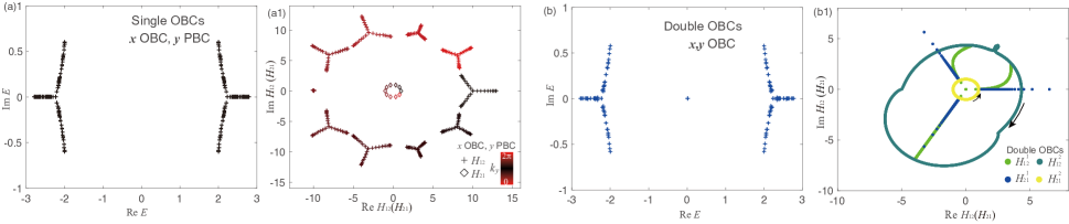
Figure S14: Energy spectrum of the 2-band model (Eq.(S76)) with (a) single OBCs and (b) double OBCs, showing double OBC topological modes that originate from a 1D topological invariant. We have $Z=z_{y}$, $\alpha=2,\beta=1,a=1,b=2$, and the constant is set to $c=5$ to make sure that the 2-band model is gapped under PBC. In (a), there is no topological zero mode, which is corroborated by the fact that $H_{12}$ in (a1) has zero winding. In (b), the presence of a double OBC topological zero mode agrees with the fact that for each of $H^{i}_{12}$ and $H^{i}_{21}$, the sum of their windings over $i=1,2$ is nonzero. The winding of $H_{12}^{2}$ is $\omega(H_{12}^{2})=-1=-\omega(H_{21}^{2})$ and $\omega(H_{12}^{1})=\omega(H_{21}^{1})=0$. Note that for the single OBC (xOBC, yPBC) case, the winding is about $k_{x}$, not $k_{y}$, so the winding of $H_{12}$ and $H_{21}$ is zero. The plots are generated with (a) $k_{y}=-\pi:\pi/30:\pi$, $L=10$, (b) with $L_{x}=L_{y}=10$.

.

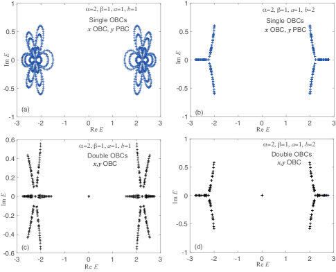
Figure S15: Energy spectrum of the 2-band model (Eq.(S76)) with $Z=z_{y}$, under single and double open boundary conditions. The Left and Right columns denote different sets of parameters (Marked in the figure). Evidently, under double OBCs, we observe topological zero modes that originate from a 1D topological invariant, indicating that the GBZ is an effective 1D GBZ, not a 2D GBZ. The constant offset in Eq.(S76) is set to $c=5$ to make sure that the 2-band model is gapped under PBCs. The system is numerically discretized such that (a,b) $k_{y}=-\pi:\pi/30:\pi$, $L_{x}=10$, (c,d) $L_{x}=L_{y}=10$.

S5 V. Generalizations to higher dimensions

Our approach for getting the correct 2D GBZs as well as their 1D constrained GBZs, if necessary, can be generalized to higher dimensions. In generic number of dimensions, the GBZ will first be symmetrically constructed in terms of relations between complex $z_{x},z_{y},z_{z},...$ and real $k_{1},k_{2},k_{3},...$. If there exist nonzero spectral windings, they will also have to be constrained to a lower dimension such that the all spectral windings in the constrained GBZ become zero.

Specializing to 3 dimensions for definiteness (higher dimension cases can be analogously written down), suppose we have

$$H_{\text{3D}}=\sum_{m,n,l}\sum_{a,b,c}t_{abc}|m,n,l\rangle\langle m+a,n+b,l+c|\ ,$$ (S82)

with hopping amplitudes $t_{abc}$ and $a,b,c$ generic integers which represent hopping directions and distances. In the same way as before, we insert the ansatz $|\psi\rangle\propto\sum_{m,n.l}\psi_{mnl}|m,n,l\rangle$ with $\psi_{m,n,l}=z_{x}^{m}z_{y}^{n}z_{z}^{l}$ into the bulk equations to obtain

$$\begin{split}E(z_{x},z_{y},z_{z})=\sum_{a,b,c}t_{abc}z_{x}^{a}z_{y}^{b}z_{z}^{c}\ .\end{split}$$ (S83)

Like before, there are generally many sets of $(z_{x},z_{y},z_{z})$ that corresponds to a particular energy $\bar{E}=E(z_{x},z_{y},z_{z})$.

To incorporate the boundary conditions, we can express a wavefunction $|\Psi\rangle$ with eigenenergy $\bar{E}=E(z_{x},z_{y},z_{z})$ as different 1D chains in the x,y or z-directions, with two other momenta as parameters:

$$\begin{split}|\Psi\rangle=|\Psi^{1}\rangle&=|\Psi^{2}\rangle=|\Psi^{3}\rangle=\ \propto\sum_{m,n,l}\Psi_{mnl}|m,n,l\rangle\ ,\\ &\Psi_{mnl}=\Psi^{1}_{mnl}=\Psi^{2}_{mnl}=\Psi^{3}_{mnl}\ ,\\ \Psi^{1}_{mn}&=\sum_{z_{y},z_{z}}\left(\sum_{j}f_{z_{x,j}}z_{x,j}^{m}\right)g_{z_{y}}z_{y}^{n}h_{z_{z}}z_{z}^{l}\ ,\\ \Psi^{2}_{mnl}&=\sum_{z_{x},z_{z}}f_{z_{x}}z_{x}^{m}\left(\sum_{j^{\prime}}{g}_{z_{y,j^{\prime}}}z_{y,j^{\prime}}^{n}\right)h_{z_{z}}z_{z}^{l}\ ,\\ \Psi^{3}_{mnl}&=\sum_{z_{x},z_{y}}f_{z_{x}}z_{x}^{m}g_{z_{y}}z_{y}^{n}\left(\sum_{j^{\prime\prime}}h_{z_{z,j^{\prime\prime}}}z_{z,j^{\prime\prime}}^{l}\right).\\ \end{split}$$ (S84)

Here $|\Psi^{1}\rangle,\ |\Psi^{2}\rangle,\ |\Psi^{3}\rangle$ are different direction decompositions of the same wave function $|\Psi\rangle$, and the first summation in the equation $\Psi^{j}_{mnl}$, $j=1,2,3$ means we must consider all the sets $z_{x},z_{y},z_{z}$ which have same energy $\bar{E}$.

Taking the different manifestations of the wave function $|\Psi\rangle$ into the boundary conditions along different directions (i.e.,${\bm{x},\bm{y},\bm{z}}$ direction), like boundary conditions along ${\bm{x}}$ direction, we have $\Psi_{m^{\prime}{n}}=\Psi^{1}_{m^{\prime}{n}}=0$ with special value $m^{\prime}$ and any values $n$, like ‘1D’ system with paramters $z_{y},z_{z}$. Thus, for a particular fixed energy, we can in general write down a relation between $z_{x}$ and $z_{y},z_{z}$, i.e.

$$\begin{split}\mathscr{F}_{1}(z_{x},z_{y},z_{z},k_{1})=0\ ,\end{split}$$ (S85)

with real $k_{1}$ “momentum” parametrizing one direction in the GBZ. In the same way, we can get other relations along ${\bm{y}},\bm{z}$ directions

$$\begin{split}\mathscr{F}_{2}(z_{x},z_{y},z_{z},k_{2})=0\ ,\end{split}$$ (S86)

$$\begin{split}\mathscr{F}_{3}(z_{x},z_{y},z_{z},k_{3})=0\ ,\end{split}$$ (S87)

with real $k_{2},k_{3}$. By construction, the $z_{x},z_{y},z_{y}$ satisfy all the boundary conditions. Hence we have 3 unknowns $z_{x},z_{y},z_{z}$ with 3 independent relational equation (Eq. S85, S86,S87), which can in principle be simultaneously solved to yield relations

$$\begin{split}z_{i}=\mathcal{F}_{i}(k_{1},k_{2},k_{3})\ ,\end{split}$$ (S88)

with $i=x,y,z$. Taking $z_{x},z_{y},z_{z}$ Eq.(S88) into the energy equation Eq.(S83), we can equivalently get the GBZ-predicted OBC energy

$$\begin{split}E(z_{x},z_{y},z_{z})=\bar{E}(k_{1},k_{2},k_{3})\ .\end{split}$$ (S89)

If the winding number of $\bar{E}(k_{1},k_{2},k_{3})$ Eq.(S83) is zero for all closed loops, the resultant GBZ of the 3D system will just be given by

$$\begin{split}\text{GBZ}_{\text{3D}}=\{z_{x},z_{y},z_{z}|z_{i}=\mathcal{F}_{i}(k_{1},k_{2},k_{3}),i=x,y,z\}\ .\end{split}$$ (S90)

And if the spectral winding number of $E(k_{1},k_{2},k_{3})$ Eq.(S89) is non-zero, we must determine what constraints we need on the parameters $k_{1},k_{2}$ and $k_{3}$ such that the spectral winding of all possible paths is zero, and that the GBZs defined by $z_{x},z_{y},z_{z}$ are periodic as we vary any of the remaining $k_{i}$. The explicit construction of such constraints to obtain the correct GBZ depends on the model, and will be the subject of future work - in the next subsection, we give a minimal example in 3D. In general, the constraints can either reduce the correct GBZ to a 2D subspace, or even a 1D subspace.

S5.0.1 Illustrative simple 3D model

For a minimal example of the GBZ construction of a 3D model, we consider 2 hopping terms in 3D space i.e.

$$H_{\text{3D}}=\sum_{m,n,l}t_{abc}|m,n,l\rangle\langle m+a,n+b,l+c|+t_{a^{\prime}b^{\prime}c^{\prime}}|m,n,l\rangle\langle m-a^{\prime},n-b^{\prime},l-c^{\prime}|\ ,$$ (S91)

with real $a,b,c,a^{\prime},b^{\prime},c^{\prime}$. Assuming the wave function ansatz $|\psi\rangle\propto\sum_{m,n.l}\psi_{mnl}|m,n,l\rangle$ with $\psi_{m,n,l}=z_{x}^{m}z_{y}^{n}z_{z}^{l}$, we arrive at two possible cases. In the first case, $a/a^{\prime}=b/b^{\prime}=c/c^{\prime}$ and previous derivations can be straightforwardly generalized to give

$$\begin{split}&\text{GBZ}_{\text{3D}}=\left\{\left.z_{x}^{a+a^{\prime}}z_{y}^{b+b^{\prime}}z_{z}^{c+c^{\prime}}=\frac{t_{a^{\prime}b^{\prime}c^{\prime}}\sin(a^{\prime}k)}{t_{abc}\sin(ak)}\text{e}^{i(a+a^{\prime})k}\right|k\in\left(-\frac{\pi}{a+a^{\prime}}\ ,\frac{\pi}{a+a^{\prime}}\right]\right\}\ ,\\ &\qquad E(z_{x},z_{y},z_{z})=E(k)=\left(\frac{t^{a^{\prime}}_{abc}t_{a^{\prime}b^{\prime}c^{\prime}}^{a}}{(\sin(ak))^{a}(\sin(a^{\prime}k))^{a^{\prime}}}\right)^{\frac{1}{a+a^{\prime}}}\sin\left((a+a^{\prime})k\right)\text{e}^{\frac{2i\pi av}{a+a^{\prime}}}\ ,\end{split}$$ (S92)

with $E(z_{x},z_{y},z_{z})=t_{abc}z_{x}^{a}z_{y}^{b}z_{z}^{c}+t_{a^{\prime}b^{\prime}c^{\prime}}z_{x}^{-a^{\prime}}z_{y}^{-b^{\prime}}z_{z}^{-c^{\prime}}$, as shown in FIG. S16 (b,b1,c,c1). In this model Eq.(S92) with $a/a^{\prime}=b/b^{\prime}=c/c^{\prime}$, the GBZ is only determined by a condition on the combination $z_{x}^{a+a^{\prime}}z_{y}^{b+b^{\prime}}z_{z}^{c+c^{\prime}}$ rather than $z_{x}$, $z_{y}$ and $z_{z}$ separately, and is akin to a 1D model along the $a\bm{x}+b\bm{y}+c\bm{z}$ direction, which is consistent with the results of numerical diagonalization, as in FIG. S3(a1—a3).

In the other case where $a/a^{\prime}=b/b^{\prime}=c/c^{\prime}$ does not hold, there is non-Bloch collapse due to uncompensated hoppings in certain directions, and the GBZ and energy are simply given by

$$\begin{split}\text{GBZ}&=\left\{z_{x}^{a+a^{\prime}}z_{y}^{b+b^{\prime}}z_{z}^{c+c^{\prime}}=-1\right\}\ ,\\ &\qquad E(z_{x},z_{y},z_{z})=0\ ,\end{split}$$ (S93)

as shown in FIG. S16 (a,a1). In both of these cases, the GBZ spectrum have zero winding number, and further dimensional reduction is not necessary.

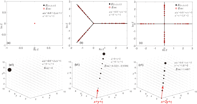
Figure S16: Spectra and illustrative eigenstates for $H_{\text{3D}}$ with different $a,b,c,a^{\prime},b^{\prime},c^{\prime}$ case. (a–c) Excellent agreement between the GBZ eigenenergies $E(z_{x},z_{y})$ of GBZ and OBC eigenenergies $E_{\text{OBC}}$ of Eq.(S91). (a1—c1) Spatial profiles for the $E_{\text{OBC}}$ eigenstate of a few other illustrative cases, clearly showing that the skin states are aligned along the ($a\bm{x}+b\bm{y}+c\bm{z}$) direction (b1,c1). The model parameters are $L_{x}=L_{y}=L_{z}=10$, $t_{abc}=1,t_{a^{\prime}b^{\prime}c^{\prime}}=2$ and the specific values of $a,b,c,a^{\prime},b^{\prime},c^{\prime}$ and $E_{\text{OBC}}$ are indicated in the figure.

In general, in arbitrarily high dimensional systems, the number of independent $z_{i}$ is always the same as the number of independent relations $\mathcal{F}_{i}$, with zero spectral winding either automatically satisfied or fulfilled via dimensional reduction to a lower-dimensional GBZ.

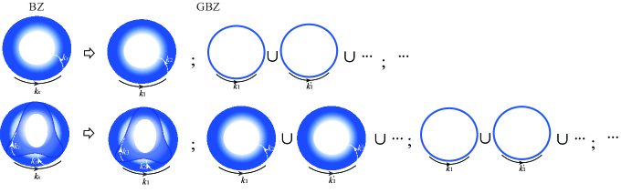
Figure S17: Schematic illustration of effective BZ for higher dimensional systems. (Top) In 2D lattices that are Hermitian or “unentangled”, the BZ is simply a 2D torus; yet for “entangled” non-Hermitian cases, the effective BZ becomes the union of one or more 1D tori. (Bottom) Similarly, 3D lattices that are Hermitian or “unentangled” have 3D tori as their BZ, but for “entangled” non-Hermitian cases, the effective BZ is in general a union of various 1D and 2D tori.

References

Lee and Fisher (1981)Patrick A Lee and Daniel S Fisher, “Anderson localization in two dimensions,” Phys.
Rev. Lett. 47, 882
(1981).
Lherbier et al. (2008)Aurélien Lherbier, Blanca Biel, Yann-Michel Niquet, and Stephan Roche, “Transport length scales in disordered graphene-based materials: Strong
localization regimes and dimensionality effects,” Phys. Rev. Lett. 100, 036803 (2008).
Aharony et al. (1976)Amnon Aharony, Yoseph Imry,
and Shang-keng Ma, “Lowering of dimensionality
in phase transitions with random fields,” Phys. Rev. Lett. 37, 1364 (1976).
Alekhin (2005)A.D. Alekhin, “Critical
indices for systems of different space dimensionality,” Journal of Molecular Liquids 120, 43–45 (2005), physics of Liquid Matter: Modern Problems.
Altland and Zirnbauer (1997)Alexander Altland and Martin R. Zirnbauer, “Nonstandard symmetry classes in mesoscopic normal-superconducting hybrid
structures,” Phys. Rev. B 55, 1142–1161 (1997).
Schnyder et al. (2008)Andreas P. Schnyder, Shinsei Ryu, Akira Furusaki, and Andreas W. W. Ludwig, “Classification of topological insulators and superconductors in three
spatial dimensions,” Phys. Rev. B 78, 195125 (2008).
Ryu et al. (2010)Shinsei Ryu, Andreas P Schnyder, Akira Furusaki, and Andreas WW Ludwig, “Topological insulators and superconductors: tenfold way and dimensional
hierarchy,” New Journal of Physics 12, 065010 (2010).
Kitaev (2009)Alexei Kitaev, “Periodic table
for topological insulators and superconductors,” in AIP conference
proceedings, Vol. 1134 (American Institute of Physics, 2009) pp. 22–30.
Morimoto and Furusaki (2013)Takahiro Morimoto and Akira Furusaki, “Topological classification with additional symmetries from clifford
algebras,” Phys. Rev. B 88, 125129 (2013).
Chiu et al. (2013)Ching-Kai Chiu, Hong Yao, and Shinsei Ryu, “Classification of
topological insulators and superconductors in the presence of reflection
symmetry,” Phys. Rev. B 88, 075142 (2013).
Gong et al. (2018)Zongping Gong, Yuto Ashida, Kohei Kawabata, Kazuaki Takasan, Sho Higashikawa, and Masahito Ueda, “Topological phases of non-hermitian systems,” Phys.
Rev. X 8, 031079
(2018).
Liu et al. (2019)Chun-Hui Liu, Hui Jiang, and Shu Chen, “Topological
classification of non-hermitian systems with reflection symmetry,” Phys. Rev. B 99, 125103 (2019).
Li et al. (2019a)Linhu Li, Ching Hua Lee, and Jiangbin Gong, “Geometric characterization
of non-hermitian topological systems through the singularity ring in
pseudospin vector space,” Phys. Rev. B 100, 075403 (2019a).
Kawabata et al. (2019)Kohei Kawabata, Ken Shiozaki, Masahito Ueda, and Masatoshi Sato, “Symmetry and
topology in non-hermitian physics,” Phys.
Rev. X 9, 041015
(2019).
Zhou and Lee (2019)Hengyun Zhou and Jong Yeon Lee, “Periodic table for
topological bands with non-hermitian symmetries,” Phys.
Rev. B 99, 235112
(2019).
Li and Mong (2021)Zhi Li and Roger SK Mong, “Homotopical
characterization of non-hermitian band structures,” Phys. Rev. B 103, 155129 (2021).
Hu and Hughes (2011)Yi Chen Hu and Taylor L Hughes, “Absence of
topological insulator phases in non-hermitian p t-symmetric hamiltonians,” Phys. Rev. B 84, 153101 (2011).
Esaki et al. (2011)Kenta Esaki, Masatoshi Sato,
Kazuki Hasebe, and Mahito Kohmoto, “Edge states and topological
phases in non-hermitian systems,” Phys.
Rev. B 84, 205128
(2011).
Lee and Chan (2014)Tony E. Lee and Ching-Kit Chan, “Heralded magnetism
in non-hermitian atomic systems,” Phys.
Rev. X 4, 041001
(2014).
Lee et al. (2014)Tony E Lee, Florentin Reiter,
and Nimrod Moiseyev, “Entanglement and spin
squeezing in non-hermitian phase transitions,” Phys. Rev. Lett. 113, 250401 (2014).
Leykam et al. (2017)Daniel Leykam, Konstantin Y. Bliokh, Chunli Huang,
Y. D. Chong, and Franco Nori, “Edge modes, degeneracies, and
topological numbers in non-hermitian systems,” Phys. Rev. Lett. 118, 040401 (2017).
Hu et al. (2017)Wenchao Hu, Hailong Wang,
Perry Ping Shum, and Y. D. Chong, “Exceptional points in a non-hermitian
topological pump,” Phys. Rev. B 95, 184306 (2017).
Lieu (2018)Simon Lieu, “Topological phases
in the non-hermitian su-schrieffer-heeger model,” Phys.
Rev. B 97, 045106
(2018).
Yin et al. (2018)Chuanhao Yin, Hui Jiang, Linhu Li,
Rong Lü, and Shu Chen, “Geometrical meaning of winding number
and its characterization of topological phases in one-dimensional chiral
non-hermitian systems,” Phys. Rev. A 97, 052115 (2018).
Jiang et al. (2018)Hui Jiang, Chao Yang, and Shu Chen, “Topological invariants and
phase diagrams for one-dimensional two-band non-hermitian systems without
chiral symmetry,” Phys. Rev. A 98, 052116 (2018).
Li et al. (2018)C. Li, X. Z. Zhang,
G. Zhang, and Z. Song, “Topological phases in a kitaev chain with
imbalanced pairing,” Phys. Rev. B 97, 115436 (2018).
Shen et al. (2018)Huitao Shen, Bo Zhen, and Liang Fu, “Topological band theory for
non-hermitian hamiltonians,” Phys. Rev. Lett. 120, 146402 (2018).
Borgnia et al. (2020)Dan S. Borgnia, Alex Jura Kruchkov, and Robert-Jan Slager, “Non-hermitian boundary modes and topology,” Phys. Rev. Lett. 124, 056802 (2020).
Pan et al. (2020)Lei Pan, Xin Chen,
Yu Chen, and Hui Zhai, “Non-hermitian linear response theory,” Nature Physics 16, 767–771 (2020).
Budich et al. (2019)Jan Carl Budich, Johan Carlström, Flore K. Kunst, and Emil J. Bergholtz, “Symmetry-protected nodal phases in non-hermitian systems,” Phys. Rev. B 99, 041406 (2019).
Qin et al. (2023a)Fang Qin, Ruizhe Shen,
Ching Hua Lee, et al., “Non-hermitian
squeezed polarons,” Physical Review A 107, L010202 (2023a).
Gao et al. (2015)Tiejun Gao, E Estrecho,
KY Bliokh, TCH Liew, MD Fraser, Sebastian Brodbeck, Martin Kamp, Christian Schneider, Sven Höfling, Y Yamamoto, et al., “Observation of non-hermitian degeneracies in a chaotic
exciton-polariton billiard,” Nature 526, 554–558 (2015).
Zeuner et al. (2015)Julia M. Zeuner, Mikael C. Rechtsman, Yonatan Plotnik, Yaakov Lumer, Stefan Nolte, Mark S. Rudner, Mordechai Segev, and Alexander Szameit, “Observation of a topological transition in the bulk of a non-hermitian
system,” Phys. Rev. Lett. 115, 040402 (2015).
Xu et al. (2016)Haitan Xu, David Mason,
Luyao Jiang, and JGE Harris, “Topological energy transfer in an
optomechanical system with exceptional points,” Nature 537, 80 (2016).
Xiao et al. (2017)L Xiao, X Zhan, ZH Bian, KK Wang, X Zhang, XP Wang, J Li, K Mochizuki, D Kim, N Kawakami, et al., “Observation of topological edge states in
parity–time-symmetric quantum walks,” Nature Physics 13, 1117–1123 (2017).
Feng et al. (2017)Liang Feng, Ramy El-Ganainy,
and Li Ge, “Non-hermitian photonics based on
parity–time symmetry,” Nature Photonics 11, 752 (2017).
Weimann et al. (2017)Steffen Weimann, Manuel Kremer, Yonatan Plotnik, Yaakov Lumer,
Stefan Nolte, Konstantinos G Makris, Mordechai Segev, Mikael C Rechtsman, and Alexander Szameit, “Topologically protected bound states in
photonic parity–time-symmetric crystals,” Nature
materials 16, 433–438
(2017).
Parto et al. (2018)Midya Parto, Steffen Wittek,
Hossein Hodaei, Gal Harari, Miguel A Bandres, Jinhan Ren, Mikael C Rechtsman, Mordechai Segev, Demetrios N Christodoulides, and Mercedeh Khajavikhan, “Edge-mode lasing in 1d
topological active arrays,” Phys. Rev. Lett. 120, 113901 (2018).
Weidemann et al. (2020)Sebastian Weidemann, Mark Kremer, Tobias Helbig, Tobias Hofmann, Alexander Stegmaier, Martin Greiter, Ronny Thomale, and Alexander Szameit, “Topological funneling of light,” Science 368, 311–314 (2020).
Helbig et al. (2020)T Helbig, T Hofmann,
S Imhof, M Abdelghany, T Kiessling, LW Molenkamp, CH Lee, A Szameit, M Greiter, and R Thomale, “Generalized bulk–boundary correspondence in non-hermitian topolectrical
circuits,” Nature Physics , 1–4
(2020).
Hofmann et al. (2020)Tobias Hofmann, Tobias Helbig, Frank Schindler, Nora Salgo,
Marta Brzezińska,
Martin Greiter, Tobias Kiessling, David Wolf, Achim Vollhardt, Anton Kabaši, et al., “Reciprocal skin effect and
its realization in a topolectrical circuit,” Physical Review Research 2, 023265 (2020).
Xiao et al. (2020)Lei Xiao, Tianshu Deng,
Kunkun Wang, Gaoyan Zhu, Zhong Wang, Wei Yi, and Peng Xue, “Non-hermitian bulk–boundary correspondence in quantum
dynamics,” Nature Physics 16, 761–766 (2020).
Zou et al. (2021)Deyuan Zou, Tian Chen,
Wenjing He, Jiacheng Bao, Ching Hua Lee, Houjun Sun, and Xiangdong Zhang, “Observation of hybrid higher-order
skin-topological effect in non-hermitian topolectrical circuits,” Nature Communications 12, 1–11 (2021).
Stegmaier et al. (2021)Alexander Stegmaier, Stefan Imhof, Tobias Helbig, Tobias Hofmann, Ching Hua Lee, Mark Kremer, Alexander Fritzsche, Thorsten Feichtner, Sebastian Klembt, Sven Höfling, et al., “Topological defect engineering and p t symmetry in non-hermitian
electrical circuits,” Phys. Rev. Lett. 126, 215302 (2021).
Wang et al. (2021)Kai Wang, Avik Dutt,
Charles C Wojcik, and Shanhui Fan, “Topological complex-energy braiding of
non-hermitian bands,” Nature 598, 59–64 (2021).
Gao et al. (2021)He Gao, Haoran Xue,
Zhongming Gu, Tuo Liu, Jie Zhu, and Baile Zhang, “Non-hermitian route to higher-order topology in an
acoustic crystal,” Nature communications 12, 1–7 (2021).
Zhang et al. (2021)Weixuan Zhang, Fengxiao Di,
Hao Yuan, Haiteng Wang, Xingen Zheng, Lu He, Houjun Sun, and Xiangdong Zhang, “Observation of non-hermitian many-body skin effects in hilbert
space,” arXiv preprint arXiv:2109.08334 (2021).
Shang et al. (2022)Ce Shang, Shuo Liu,
Ruiwen Shao, Peng Han, Xiaoning Zang, Xiangliang Zhang, Khaled Nabil Salama, Wenlong Gao, Ching Hua Lee, Ronny Thomale, et al., “Experimental identification of the
second-order non-hermitian skin effect with physics-graph-informed machine
learning,” arXiv preprint arXiv:2203.00484 (2022).
Weidemann et al. (2022)Sebastian Weidemann, Mark Kremer, Stefano Longhi, and Alexander Szameit, “Topological triple phase transition in non-hermitian floquet
quasicrystals,” Nature 601, 354–359 (2022).
Li et al. (2022)Haowei Li, Xiaoling Cui, and Wei Yi, “Non-hermitian skin effect in a
spin-orbit-coupled bose-einstein condensate,” arXiv preprint arXiv:2201.01580 (2022).
Zhang et al. (2022a)Xiao Zhang, Boxue Zhang,
Weihong Zhao, and Ching Hua Lee, “Observation of non-local
impedance response in a passive electrical circuit,” arXiv preprint arXiv:2211.09152 (2022a).
Rosa-Medina et al. (2022)Rodrigo Rosa-Medina, Francesco Ferri, Fabian Finger,
Nishant Dogra, Katrin Kroeger, Rui Lin, R Chitra, Tobias Donner, and Tilman Esslinger, “Observing dynamical currents in a non-hermitian momentum lattice,” Phys. Rev. Lett. 128, 143602 (2022).
Zhang et al. (2023a)Hanxu Zhang, Tian Chen,
Linhu Li, Ching Hua Lee, and Xiangdong Zhang, “Electrical circuit realization of
topological switching for the non-hermitian skin effect,” Physical Review B 107, 085426 (2023a).
Thouless et al. (1982)D. J. Thouless, M. Kohmoto,
M. P. Nightingale, and M. den Nijs, “Quantized hall conductance in a
two-dimensional periodic potential,” Phys.
Rev. Lett. 49, 405–408
(1982).
Qi et al. (2008)Xiao-Liang Qi, Taylor L Hughes, and Shou-Cheng Zhang, “Topological field
theory of time-reversal invariant insulators,” Phys.
Rev. B 78, 195424
(2008).
Schindler et al. (2018)Frank Schindler, Ashley M Cook, Maia G Vergniory, Zhijun Wang, Stuart SP Parkin, B Andrei Bernevig, and Titus Neupert, “Higher-order
topological insulators,” Science advances 4, eaat0346 (2018).
Lee et al. (2018a)Ching Hua Lee, Guangjie Li, Yuhan Liu, Tommy Tai,
Ronny Thomale, and Xiao Zhang, “Tidal surface states as fingerprints of
non-hermitian nodal knot metals,” arXiv preprint arXiv:1812.02011 (2018a).
Lee et al. (2019)Ching Hua Lee, Linhu Li, and Jiangbin Gong, “Hybrid
higher-order skin-topological modes in nonreciprocal systems,” Phys. Rev. Lett. 123, 016805 (2019).
Luo and Zhang (2019)Xi-Wang Luo and Chuanwei Zhang, “Higher-order
topological corner states induced by gain and loss,” Phys. Rev. Lett. 123, 073601 (2019).
Tuloup et al. (2020)Thomas Tuloup, Raditya Weda Bomantara, Ching Hua Lee, and Jiangbin Gong, “Nonlinearity
induced topological physics in momentum space and real space,” Physical Review B 102, 115411 (2020).
Jiang and Lee (2022)Hui Jiang and Ching Hua Lee, “Filling up complex
spectral regions through non-hermitian disordered chains,” Chinese Physics B 31, 050307 (2022).
Note (1)This may not be the case for hyperbolic lattices Maciejko and Rayan (2021, 2022); Boettcher et al. (2022)
, which can be realized in circuit setups Kollár et al. (2019); Boettcher et al. (2020); Lenggenhager et al. (2021).
Zhang et al. (2022b)Xiujuan Zhang, Tian Zhang,
Ming-Hui Lu, and Yan-Feng Chen, “A review on non-hermitian
skin effect,” Advances in Physics: X 7, 2109431 (2022b).
Lin et al. (2023)Rijia Lin, Tommy Tai,
Linhu Li, and Ching Hua Lee, “Topological non-hermitian skin
effect,” Frontiers of Physics 18, 53605 (2023).
Yao and Wang (2018)Shunyu Yao and Zhong Wang, “Edge states and topological
invariants of non-hermitian systems,” Phys. Rev. Lett. 121, 086803 (2018).
Lee and Thomale (2019)Ching Hua Lee and Ronny Thomale, “Anatomy of skin modes and topology in non-hermitian systems,” Phys. Rev. B 99, 201103 (2019).
Song et al. (2019a)Fei Song, Shunyu Yao, and Zhong Wang, “Non-hermitian topological
invariants in real space,” Phys. Rev. Lett. 123, 246801 (2019a).
Song et al. (2019b)Fei Song, Shunyu Yao, and Zhong Wang, “Non-hermitian skin effect
and chiral damping in open quantum systems,” Phys. Rev. Lett. 123, 170401 (2019b).
Zhang et al. (2020)Kai Zhang, Zhesen Yang, and Chen Fang, “Correspondence between
winding numbers and skin modes in non-hermitian systems,” Phys. Rev. Lett. 125, 126402 (2020).
Yokomizo and Murakami (2019)Kazuki Yokomizo and Shuichi Murakami, “Non-bloch band
theory of non-hermitian systems,” Phys. Rev. Lett. 123, 066404 (2019).
Yang et al. (2020)Zhesen Yang, Kai Zhang,
Chen Fang, and Jiangping Hu, “Non-hermitian bulk-boundary
correspondence and auxiliary generalized brillouin zone theory,” Phys. Rev. Lett. 125, 226402 (2020).
Lee and Longhi (2020)Ching Hua Lee and Stefano Longhi, “Ultrafast and anharmonic rabi oscillations between non-bloch bands,” Communications Physics 3, 1–9 (2020).
Claes and Hughes (2021a)Jahan Claes and Taylor L. Hughes, “Skin effect and
winding number in disordered non-hermitian systems,” Phys. Rev. B 103, L140201 (2021a).
Okuma et al. (2020)Nobuyuki Okuma, Kohei Kawabata, Ken Shiozaki, and Masatoshi Sato, “Topological origin of non-hermitian skin effects,” Phys. Rev. Lett. 124, 086801 (2020).
Schindler and Prem (2021)Frank Schindler and Abhinav Prem, “Dislocation
non-hermitian skin effect,” Phys. Rev. B 104, L161106 (2021).
Okuma and Sato (2021)Nobuyuki Okuma and Masatoshi Sato, “Non-hermitian skin effects in hermitian correlated or disordered systems:
Quantities sensitive or insensitive to boundary effects and
pseudo-quantum-number,” Phys. Rev. Lett. 126, 176601 (2021).
Li et al. (2021b)Linhu Li, Sen Mu, Ching Hua Lee, and Jiangbin Gong, “Quantized classical response from
spectral winding topology,” Nature communications 12, 1–11 (2021b).
Guo et al. (2021)Cui-Xian Guo, Chun-Hui Liu, Xiao-Ming Zhao, Yanxia Liu, and Shu Chen, “Exact solution of
non-hermitian systems with generalized boundary conditions: Size-dependent
boundary effect and fragility of the skin effect,” Phys. Rev. Lett. 127, 116801 (2021).
Yang et al. (2022)Russell Yang, Jun Wei Tan,
Tommy Tai, Jin Ming Koh, Linhu Li, Stefano Longhi, and Ching Hua Lee, “Designing non-hermitian real spectra through electrostatics,” Science Bulletin 67, 1865–1873 (2022).
Rafi-Ul-Islam et al. (2022a)SM Rafi-Ul-Islam, Zhuo Bin Siu, Haydar Sahin,
Ching Hua Lee, and Mansoor BA Jalil, “System size dependent
topological zero modes in coupled topolectrical chains,” Physical Review B 106, 075158 (2022a).
Zhang et al. (2022c)Boxue Zhang, Qingya Li,
Xiao Zhang, and Ching Hua Lee, “Real non-hermitian energy
spectra without any symmetry,” Chinese Physics B 31, 070308 (2022c).
Rafi-Ul-Islam et al. (2022b)SM Rafi-Ul-Islam, Zhuo Bin Siu, Haydar Sahin,
Ching Hua Lee, and Mansoor BA Jalil, “Critical hybridization of
skin modes in coupled non-hermitian chains,” Physical Review Research 4, 013243 (2022b).
Gu et al. (2022)Zhongming Gu, He Gao, Haoran Xue,
Jensen Li, Zhongqing Su, and Jie Zhu, “Transient non-hermitian skin effect,” Nature
Communications 13, 7668
(2022).
Okugawa et al. (2020)Ryo Okugawa, Ryo Takahashi, and Kazuki Yokomizo, “Second-order
topological non-hermitian skin effects,” Phys. Rev. B 102, 241202 (2020).
Claes and Hughes (2021b)Jahan Claes and Taylor L. Hughes, “Skin effect and
winding number in disordered non-hermitian systems,” Phys. Rev. B 103, L140201 (2021b).
Qin et al. (2023b)Fang Qin, Ye Ma, Ruizhe Shen, Ching Hua Lee, et al., “Universal competitive spectral scaling
from the critical non-hermitian skin effect,” Physical Review B 107, 155430 (2023b).
Lei et al. (2023)Zhoutao Lei, Ching Hua Lee, and Linhu Li, “Pt-activated non-hermitian
skin modes,” arXiv preprint arXiv:2304.13955 (2023).
Guo et al. (2023)Taozhi Guo, Kohei Kawabata,
Ryota Nakai, and Shinsei Ryu, “Non-hermitian boost deformation,” arXiv preprint
arXiv:2301.05973 (2023).
Note (2)Which arises even if all couplings are local.
Lee et al. (2020a)Ching Hua Lee, Linhu Li, Ronny Thomale, and Jiangbin Gong, “Unraveling non-hermitian
pumping: Emergent spectral singularities and anomalous responses,” Phys. Rev. B 102, 085151 (2020a).
Bachtold et al. (1999)Adrian Bachtold, Christoph Strunk, Jean-Paul Salvetat, Jean-Marc Bonard, Laszló Forró, Thomas Nussbaumer, and Christian Schönenberger, “Aharonov–bohm oscillations in carbon nanotubes,” Nature 397, 673–675
(1999).
Gou et al. (2020)Wei Gou, Tao Chen,
Dizhou Xie, Teng Xiao, Tian-Shu Deng, Bryce Gadway, Wei Yi, and Bo Yan, “Tunable non-reciprocal quantum transport through a
dissipative aharonov-bohm ring in ultracold atoms,” Phys. Rev. Lett. 124, 070402 (2020).
Hatano and Nelson (1996)Naomichi Hatano and David R. Nelson, “Localization transitions in non-hermitian quantum mechanics,” Phys. Rev. Lett. 77, 570–573 (1996).
Hatano and Nelson (1997)Naomichi Hatano and David R. Nelson, “Vortex pinning and non-hermitian quantum mechanics,” Phys.
Rev. B 56, 8651–8673
(1997).
Longhi et al. (2015)Stefano Longhi, Davide Gatti,
and Giuseppe Della Valle, “Non-hermitian transparency and one-way transport in low-dimensional lattices
by an imaginary gauge field,” Phys. Rev. B 92, 094204 (2015).
Liu et al. (2020a)Chun-Hui Liu, Kai Zhang, Zhesen Yang, and Shu Chen, “Helical damping and
dynamical critical skin effect in open quantum systems,” Physical Review Research 2, 043167 (2020a).
Yokomizo and Murakami (2021)Kazuki Yokomizo and Shuichi Murakami, “Scaling rule
for the critical non-hermitian skin effect,” Phys. Rev. B 104, 165117 (2021).
Kawabata et al. (2022)Kohei Kawabata, Tokiro Numasawa, and Shinsei Ryu, “Entanglement phase
transition induced by the non-hermitian skin effect,” arXiv preprint arXiv:2206.05384 (2022).
Note (3)This can also be seen via a complex flux threading Gedankan
experiment Xiong (2018); Lee and Thomale (2019); Li et al. (2021b). Gauge
transforming all flux onto the boundary coupling, the latter shrinks
when we ramp up ; correspondingly, the effect of
cycling across diminishes. In the
OBC limit, further spectral flow is not possible, and only degenerate
spectral loops can exist.
Note (4)We refer to it as the type-III model in Sect. III of our
Supplement, where we also explained why it undergoes nontrivial dimensional
transmutation, but not related models.
(123)“Supplemental materials, which
also includes
refs. Kohn (1959); He and Vanderbilt (2001); Lee and Ye (2015); Crespi et al. (2013); Ningyuan et al. (2015); Ezawa (2019); Zhang et al. (2023b),” .
Lee and Qi (2014)Ching Hua Lee and Xiao-Liang Qi, “Lattice
construction of pseudopotential hamiltonians for fractional chern
insulators,” Phys. Rev. B 90, 085103
(2014).
Groenendijk et al. (2021)Solofo Groenendijk, Thomas L Schmidt, and Tobias Meng, “Universal hall
conductance scaling in non-hermitian chern insulators,” Physical Review Research 3, 023001 (2021).
Tantivasadakarn (2017)Nathanan Tantivasadakarn, “Dimensional reduction and topological invariants of
symmetry-protected topological phases,” Phys.
Rev. B 96, 195101
(2017).
Gu et al. (2016)Yingfei Gu, Ching Hua Lee,
Xueda Wen, Gil Young Cho, Shinsei Ryu, and Xiao-Liang Qi, “Holographic duality between (2+1)-dimensional
quantum anomalous hall state and (3+1)-dimensional topological insulators,” Phys. Rev. B 94, 125107 (2016).
Hu et al. (2020)Hong-Ye Hu, Shuo-Hui Li,
Lei Wang, and Yi-Zhuang You, “Machine learning holographic mapping by
neural network renormalization group,” Physical Review Research 2, 023369 (2020).
Botten et al. (1997)LC Botten, RC McPhedran,
NA Nicorovici, and GH Derrick, “Periodic models for thin optimal
absorbers of electromagnetic radiation,” Phys.
Rev. B 55, R16072
(1997).
Lee et al. (2018b)Ching Hua Lee, Stefan Imhof, Christian Berger, Florian Bayer,
Johannes Brehm, Laurens W Molenkamp, Tobias Kiessling, and Ronny Thomale, “Topolectrical circuits,” Communications Physics 1, 1–9 (2018b).
Imhof et al. (2018)Stefan Imhof, Christian Berger, Florian Bayer,
Johannes Brehm, Laurens W Molenkamp, Tobias Kiessling, Frank Schindler, Ching Hua Lee, Martin Greiter, Titus Neupert, et al., “Topolectrical-circuit realization of
topological corner modes,” Nature Physics 14, 925 (2018).
Helbig et al. (2019)Tobias Helbig, Tobias Hofmann, Ching Hua Lee, Ronny Thomale,
Stefan Imhof, Laurens W Molenkamp, and Tobias Kiessling, “Band structure engineering
and reconstruction in electric circuit networks,” Phys.
Rev. B 99, 161114
(2019).
Hofmann et al. (2019)Tobias Hofmann, Tobias Helbig, Ching Hua Lee,
Martin Greiter, and Ronny Thomale, “Chiral voltage propagation
and calibration in a topolectrical chern circuit,” Phys. Rev. Lett. 122, 247702 (2019).
Zhang et al. (2019)Zhi-Qiang Zhang, Bing-Lan Wu, Juntao Song, and Hua Jiang, “Topological
anderson insulator in electric circuits,” Phys. Rev. B 100, 184202 (2019).
Ni et al. (2020)Xiang Ni, Zhicheng Xiao,
Alexander B Khanikaev, and Andrea Alù, “Robust multiplexing with
topolectrical higher-order chern insulators,” Phys. Rev. Applied 13, 064031 (2020).
Lee et al. (2020b)Ching Hua Lee, Amanda Sutrisno, Tobias Hofmann, Tobias Helbig, Yuhan Liu,
Yee Sin Ang, Lay Kee Ang, Xiao Zhang, Martin Greiter, and Ronny Thomale, “Imaging nodal knots in momentum space through
topolectrical circuits,” Nature communications 11, 1–13 (2020b).
Li et al. (2019b)Linhu Li, Ching Hua Lee, and Jiangbin Gong, “Emergence and full
3d-imaging of nodal boundary seifert surfaces in 4d topological matter,” Communications
physics 2, 135 (2019b).
Zhang and Franz (2020)Xiao-Xiao Zhang and Marcel Franz, “Non-hermitian exceptional landau quantization in electric circuits,” Phys. Rev. Lett. 124, 046401 (2020).
Lenggenhager et al. (2021)Patrick M Lenggenhager, Alexander Stegmaier, Lavi K Upreti, Tobias Hofmann, Tobias Helbig, Achim Vollhardt, Martin Greiter, Ching Hua Lee, Stefan Imhof, Hauke Brand,
et al., “Electric-circuit realization of a hyperbolic drum,” arXiv preprint arXiv:2109.01148 (2021).
Liu et al. (2021)Shuo Liu, Ruiwen Shao,
Shaojie Ma, Lei Zhang, Oubo You, Haotian Wu, Tie Cui, and Shuang Zhang, “Non-hermitian skin effect in a non-hermitian electrical circuit,” Research 2021, 1–9
(2021).
Liu et al. (2020b)Shuo Liu, Shaojie Ma,
Cheng Yang, Lei Zhang, Wenlong Gao, Yuan Jiang Xiang, Tie Jun Cui, and Shuang Zhang, “Gain- and loss-induced topological insulating
phase in a non-hermitian electrical circuit,” Phys. Rev. Applied 13, 014047 (2020b).
Hohmann et al. (2022)Hendrik Hohmann, Tobias Hofmann, Tobias Helbig, Stefan Imhof,
Hauke Brand, Lavi K Upreti, Alexander Stegmaier, Alexander Fritzsche, Tobias Müller, Udo Schwingenschlögl, et al., “Observation of cnoidal wave
localization in non-linear topolectric circuits,” arXiv preprint arXiv:2206.09931 (2022).
Wu et al. (2022)Jien Wu, Xueqin Huang,
Yating Yang, Weiyin Deng, Jiuyang Lu, Wenji Deng, and Zhengyou Liu, “Non-hermitian second-order topology induced by
resistances in electric circuits,” Physical Review B 105, 195127 (2022).
Zhu et al. (2023)Penghao Zhu, Xiao-Qi Sun,
Taylor L Hughes, and Gaurav Bahl, “Higher rank chirality and non-hermitian
skin effect in a topolectrical circuit,” Nature communications 14, 720 (2023).
Choo et al. (2018)Kenny Choo, Curt W Von Keyserlingk, Nicolas Regnault, and Titus Neupert, “Measurement of
the entanglement spectrum of a symmetry-protected topological state using the
ibm quantum computer,” Phys. Rev. Lett. 121, 086808 (2018).
Smith et al. (2019)Adam Smith, MS Kim, Frank Pollmann, and Johannes Knolle, “Simulating quantum many-body dynamics on
a current digital quantum computer,” npj Quantum Information 5, 1–13 (2019).
Behera et al. (2019)Bikash K Behera, Tasnum Reza, Angad Gupta, and Prasanta K Panigrahi, “Designing
quantum router in ibm quantum computer,” Quantum Information Processing 18, 1–13 (2019).
Azses et al. (2020)Daniel Azses, Rafael Haenel,
Yehuda Naveh, Robert Raussendorf, Eran Sela, and Emanuele G Dalla Torre, “Identification of
symmetry-protected topological states on noisy quantum computers,” Phys. Rev. Lett. 125, 120502 (2020).
Koh et al. (2022a)Jin Ming Koh, Tommy Tai, Yong Han Phee,
Wei En Ng, and Ching Hua Lee, “Stabilizing multiple
topological fermions on a quantum computer,” npj Quantum Information 8, 1–10 (2022a).
Koh et al. (2022b)Jin Ming Koh, Tommy Tai, and Ching Hua Lee, “Simulation of
interaction-induced chiral topological dynamics on a digital quantum
computer,” Physical Review Letters 129, 140502 (2022b).
Smith et al. (2022)Adam Smith, Bernhard Jobst,
Andrew G Green, and Frank Pollmann, “Crossing a topological phase
transition with a quantum computer,” Physical Review Research 4, L022020 (2022).
Koh et al. (2023)Jin Ming Koh, Tommy Tai, and Ching Hua Lee, “Observation of
higher-order topological states on a quantum computer,” arXiv preprint arXiv:2303.02179 (2023).
Shi et al. (2022)Yun-Hao Shi, Yu Liu, Yu-Ran Zhang, Zhongcheng Xiang, Kaixuan Huang, Tao Liu, Yong-Yi Wang, Jia-Chi Zhang, Cheng-Lin Deng, Gui-Han Liang, et al., “Observing topological zero modes on a 41-qubit
superconducting processor,” arXiv preprint arXiv:2211.05341 (2022).
Boettcher et al. (2022)Igor Boettcher, Alexey V Gorshkov, Alicia J Kollár, Joseph Maciejko, Steven Rayan, and Ronny Thomale, “Crystallography
of hyperbolic lattices,” Phys. Rev. B 105, 125118 (2022).
Kollár et al. (2019)Alicia J Kollár, Mattias Fitzpatrick, and Andrew A Houck, “Hyperbolic lattices in circuit quantum electrodynamics,” Nature 571, 45–50 (2019).
Boettcher et al. (2020)Igor Boettcher, Przemyslaw Bienias, Ron Belyansky, Alicia J Kollár, and Alexey V Gorshkov, “Quantum simulation of hyperbolic space with circuit quantum electrodynamics:
From graphs to geometry,” Phys. Rev. A 102, 032208 (2020).
Kohn (1959)Walter Kohn, “Analytic
properties of bloch waves and wannier functions,” Physical Review 115, 809 (1959).
He and Vanderbilt (2001)Lixin He and David Vanderbilt, “Exponential
decay properties of wannier functions and related quantities,” Phys. Rev. Lett. 86, 5341 (2001).
Lee and Ye (2015)Ching Hua Lee and Peng Ye, “Free-fermion entanglement spectrum through wannier interpolation,” Phys. Rev. B 91, 085119 (2015).
Crespi et al. (2013)Andrea Crespi, Giacomo Corrielli, Giuseppe Della Valle, Roberto Osellame, and Stefano Longhi, “Dynamic band
collapse in photonic graphene,” New Journal of Physics 15, 013012 (2013).
Ningyuan et al. (2015)Jia Ningyuan, Clai Owens,
Ariel Sommer, David Schuster, and Jonathan Simon, “Time-and site-resolved dynamics in a
topological circuit,” Phys. Rev. X 5, 021031 (2015).
Ezawa (2019)Motohiko Ezawa, “Non-hermitian higher-order topological states in nonreciprocal and
reciprocal systems with their electric-circuit realization,” Phys. Rev. B 99, 201411 (2019).
Zhang et al. (2023b)Xiao Zhang, Boxue Zhang,
Haydar Sahin, Zhuo Bin Siu, SM Rafi-Ul-Islam, Jian Feng Kong, Bing Shen, Mansoor BA Jalil, Ronny Thomale, and Ching Hua Lee, “Anomalous fractal scaling in two-dimensional electric networks,” Communications
Physics 6, 151 (2023b).
Supplementary Materials