Classical vs quantum corrections to jet broadening in a weakly-coupled Quark-Gluon Plasma

Abstract

The transverse momentum broadening coefficient $\hat{q}$ receives both soft, classical and radiative, quantum corrections. The former are responsible for a large $\mathcal{O}(g)$ correction, whereas the latter enter at relative order $\alpha_{s}$, but are enhanced by a double logarithm of the length of the medium over the thermal wavelength. We analyze radiative corrections for a weakly-coupled quark-gluon plasma. We find that a thermal population of dynamical gluons changes the boundaries and reduces the size of the double-logarithmic phase space. It also provides new subdominant logarithmic corrections. We also show how the quantum, double-logarithmic and classical, soft phase spaces are smoothly connected once the radiated gluon becomes soft enough. Finally, we discuss a pathway to a determination of radiative corrections beyond the harmonic-oscillator approximation.

1 Introduction

The highly-energetic, collimated partons that seed a jet undergo transverse momentum broadening as they propagate through the hot QCD medium that is understood to be formed in heavy-ion collisions. This broadening is described by the broadening rate, or the associated probability and the transverse momentum broadening coefficient $\hat{q}\equiv\langle k_{\perp}^{2}\rangle/L$, which describes how much transverse momentum $k_{\perp}$ is picked up per length $L$ by a highly energetic parton propagating through a plasma. The precise characterization of these quantities is thus at the forefront of theoretical and experimental investigation of this medium. We refer to Connors:2017ptx ; Cao:2020wlm ; Cunqueiro:2021wls ; Apolinario:2022vzg for recent reviews and to Burke:2013yra ; Andres:2016evc ; Xie:2019oxg ; Huss:2020whe ; Jetscape:2021ehl ; Han:2022zxn ; Xie:2022ght for extractions of $\hat{q}$ from data.

In a weakly-coupled quark-gluon plasma (QGP), $\hat{q}$ is dominated by Coulomb elastic scatterings with light partonic medium constituents, $\hat{q}=\int d^{2}k_{\perp}\,k_{\perp}^{2}\,d\Gamma_{\mathrm{el}}/d^{2}k_{\perp}$. For $k_{\perp}\sim T$ the elastic, differential scattering rate $d\Gamma_{\mathrm{el}}/d^{2}k_{\perp}$ is of order $g^{4}T^{3}/k_{\perp}^{4}$, with $T^{3}$ the (parametric) light parton density multiplying the Coulomb cross section. The resulting logarithmic integral is cut off in the infrared (IR) by dynamical screening, encoded in Hard Thermal Loop (HTL) resummation Braaten:1989mz at the soft scale $gT$. Ultraviolet (UV) regularization is also needed, as we shall explain later. The soft ($k_{\perp}\sim gT$) and thermal ($k_{\perp}\sim T$) contributions were obtained in Aurenche:2002pd and Arnold:2008vd respectively, and they combine to give $\hat{q}\sim g^{4}T^{3}$ (up to logarithms).

This leading-order (LO) contribution from the soft scale is the first signal of potentially large corrections arising from this region. Soft gluons with frequency $\omega\ll T$ are distributed on the infrared tail of the Bose–Einstein distribution, $n_{\mathrm{B}}(\omega\ll T)\approx T/\omega\gg 1$. This has two consequences: for soft, $\omega\sim gT$ modes, $T/\omega\sim 1/g$ changes the standard $g^{2}$ loop expansion into a $g$ expansion. For ultrasoft (US) modes, $\omega\sim g^{2}T$, the perturbative expansion breaks down Linde:1980ts , but their contribution only enters $\hat{q}$ at relative order $g^{2}$ Laine:2012ht . The second consequence is that this large occupation number implies the classical nature of these contributions.

In a pioneering study, Caron-Huot showed in CaronHuot:2008ni that these classical plasma effects can be mapped, for the observable at hand, to three-dimensional, Euclidean physics described by Electrostatic QCD (EQCD) Braaten:1994na ; Braaten:1995cm ; Braaten:1995jr ; Kajantie:1995dw ; Kajantie:1997tt . This paved the way first to the perturbative determination of the $\mathcal{O}(g)$ next-to-leading order (NLO) correction to $\hat{q}$, presented in CaronHuot:2008ni itself, without recurring to brute-force numerical computations in the HTL theory. Second, it was used for non-perturbative determinations of the transverse scattering rate using lattice EQCD Panero:2013pla ; Moore:2019lgw — see also Laine:2013lia — thus incorporating to all orders the contribution of classical soft and ultrasoft modes. The impact of this non-perturbative rate on medium-induced emission was examined in Moore:2021jwe ; Schlichting:2021idr and found to be very relevant.

Over the past decade, another source of potentially large higher-order corrections to $\hat{q}$ has been discovered Wu:2011kc ; Liou:2013qya ; Blaizot:2013vha — see Blaizot:2015lma for a review. These are quantum, radiative corrections, arising from keeping track of the recoil during the medium-induced emission of a gluon. These corrections, while suppressed by a factor of $g^{2}$, feature a double-logarithmic enhancement, whose argument was found to be $L_{\mathrm{med}}/\tau_{\mathrm{min}}$, with $L_{\mathrm{med}}$ the length of the medium and $\tau_{\mathrm{min}}\sim 1/T$ for a thermal medium. This potentially large double logarithm can then be resummed, effectively renormalizing the leading-order value of $\hat{q}$. The evolution equations for the logarithmic resummation were analyzed in Iancu:2014kga ; Iancu:2014sha and recently solved numerically in Caucal:2021lgf ; Caucal:2022fhc , whereas the change in the argument of the double logarithm from a dense to a dilute medium was studied in Blaizot:2019muz . Blaizot:2014bha ; Wu:2014nca ; Iancu:2014kga showed that when two collinear gluons are emitted with overlapping formation times the same physics is responsible for double-logarithmic corrections, which are thus universal. This same problem is being analyzed in full detail, beyond the double-logarithmic terms, in Arnold:2015qya ; Arnold:2016kek ; Arnold:2016mth ; Arnold:2018yjd ; Arnold:2018fjr ; Arnold:2019qqc ; Arnold:2020uzm ; Arnold:2021pin ; Arnold:2022epx . Arnold:2021mow found that the single-logarithmic corrections too are related by the same universality to those determined for $\hat{q}$ in Liou:2013qya .

The presence of two such large corrections, the classical ones at order $g$ and beyond, and the quantum radiative ones at order $g^{2}\ln^{2}(L_{\mathrm{med}}T)$, together with the recent developments on both sides, such as the present availability of high-quality non-perturbative data for the classical corrections, naturally begs the question of which of the two corrections, if any, can be considered parametrically larger than the other.

Motivated by this question, in this paper we address the connection of the two corrections in the case of a weakly-coupled quark-gluon plasma. We will revisit the calculation of radiative corrections with full accounting of the thermal length and momentum scales. We shall show how the effect of Bose enhancement for the radiated gluon, as well as the possibility of absorption of thermal gluons — neither was included in previous analyses — modifies the shape of the double-log-enhanced region in the frequency–formation time plane, thus changing the argument of the double logarithm. On a more technical standpoint, we also show how the regions giving rise to classical and quantum corrections meet at their shared boundary, and how this can be rephrased in terms of the mapping to the Euclidean 3D theory introduced by Caron-Huot.

Our analysis will be mostly limited to the largest double-logarithmic corrections only and it will adopt the so-called harmonic-oscillator approximation: we shall discuss some smaller corrections and provide a pathway to the determinations of missing ones.

The paper is organized as follows: in Sec. 2 we review the determination of double-log-enhanced radiative corrections. In Sec. 3 we show how this derivation needs to be modified to account for the presence of a weakly-coupled dynamical medium and we present there our main results. In Sec. 4 we provide, for the interested readers, more details on our derivations and on the connection to the classical regime of Caron-Huot, while in Sec. 5 we provide a pathway towards the investigation of radiative corrections beyond the harmonic-oscillator and double-logarithmic approximations. Finally, in Sec. 6 we draw our conclusions. Our conventions, as well as more technical detail on the calculations, are collected in the appendices.

2 The double-logarithmic phase space in the literature

As our starting point, let us call $\mathcal{C}(k_{\perp})$ the differential-in-transverse-momentum scattering rate, also known as scattering kernel, i.e.

$$\mathcal{C}(k_{\perp})\equiv(2\pi)^{2}\frac{d\Gamma}{d^{2}k_{\perp}},\,\qquad\hat{q}(\mu)=\int^{\mu}\frac{d^{2}k_{\perp}}{(2\pi)^{2}}k_{\perp}^{2}\,\mathcal{C}(k_{\perp})\,,$$ (1)

where $\frac{d\Gamma}{d^{2}k_{\perp}}$ is the rate for the hard jet parton of energy $E\gg T$ and momentum along $z$ to acquire $k_{\perp}$ transverse momentum — see App. A for our conventions.

$\mu$ is some process-dependent UV regularisation for the Coulomb logarithm in the leading-order scattering kernel, $\mathcal{C}(k_{\perp})\propto k_{\perp}^{-4}$ for $k_{\perp}\gg gT$. We shall treat $\mu$ as a parameter, without necessarily identifying it with the saturation scale $Q_{s}^{2}=\hat{q}L_{\mathrm{med}}$ as done in Liou:2013qya . In the case of QCD, asymptotic freedom would in principle make the integration UV-finite, but it would include in $\hat{q}$ Molière scattering Moliere:1947zza ; Moliere:1948zz , i.e. very large momentum transfers, which necessarily give rise to two hard jet partons in the final state, in what is no longer a diffusive process — see e.g. DEramo:2018eoy ; Dai:2020rlu . This $\mu$ factorisation also allows the incorporation in the effective kinetic description of Arnold:2002zm ; Ghiglieri:2015ala , where $\hat{q}(\mu)$ is (one of) the transport coefficients describing diffusive momentum exchanges at scales below $\mu$. There it is complemented by the full kinetic description above that cutoff.

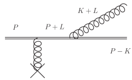
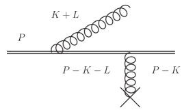
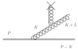
Figure 1: Diagrams contributing to radiative momentum broadening in the single-scattering regime. The double solid line represents the hard jet parton (quark or gluon), curly lines are gluons and the cross is a quark or gluon scattering center in the medium.

We now consider the radiative correction to the transverse scattering rate in the single-scattering regime, which emerges naturally in the standard dipole picture Liou:2013qya . It comes from the diagrams in Fig. 1 and it reads

$$\delta\mathcal{C}(k_{\perp})_{\mathrm{rad}}^{N=1}=4\alpha_{s}C_{R}\int\frac{dk^{+}}{k^{+}}\int\frac{d^{2}l_{\perp}}{(2\pi)^{2}}\mathcal{C}_{0}(l_{\perp})\frac{l_{\perp}^{2}}{k_{\perp}^{2}(\bm{l}_{\perp}+\bm{k}_{\perp})^{2}},$$ (2)

where $C_{R}$ is the Casimir factor of the hard jet parton, $C_{R}=C_{F}=(N_{c}^{2}-1)/2N_{c}$ for a quark, $C_{R}=C_{A}=N_{c}$ for a gluon. As shown in Fig 1, $P$ is the four-momentum of the hard jet parton, with $p^{0}=p^{z}=E\gg T$. $L$ denotes the four-momentum acquired from the medium, and $K$ is chosen in such a way that the hard jet parton acquires a final transverse momentum of modulus $k_{\perp}$. $k^{+}\equiv(k^{0}+k^{z})/2\approx k^{0}$ is the light-cone frequency — see App. A for our conventions. $l_{\perp}^{2}/(k_{\perp}^{2}(\bm{l}_{\perp}+\bm{k}_{\perp})^{2})$ is then the standard dipole factor and $2C_{R}/k^{+}$ the soft limit of the $g\leftarrow R$ DGLAP splitting function. Finally, $\mathcal{C}_{0}(l_{\perp})\sim g^{4}C_{A}T^{3}/l_{\perp}^{4}$ is the leading order scattering rate from a gluon source. In App. B we list the known LO results for $m_{D}\lesssim l_{\perp}\ll T$ and for $l_{\perp}\gtrsim T$, as well as a smooth interpolating scheme Aurenche:2002pd ; Arnold:2008vd . For the present discussion the precise form is irrelevant, as we shall soon see.

Eq. (2) is in principle just the first, $N=1$ term in the opacity series of multiple scattering. As observed in Liou:2013qya , the requirement that the transverse momentum carried away by the gluon is larger than that picked up in a typical collision with the medium, $|\bm{k}_{\perp}+\bm{l}_{\perp}|\gg l_{\perp}$, puts us in the single-scattering regime, where the $N=1$ term dominates. This yields

$$\delta\mathcal{C}(k_{\perp})_{\mathrm{rad}}^{\mathrm{single}}=4\alpha_{s}C_{R}\,\hat{q}_{0}\int\frac{dk^{+}}{k^{+}}\frac{1}{k_{\perp}^{4}}\,,\qquad\text{with}\quad\hat{q}_{0}\equiv\int^{\rho}\frac{d^{2}l_{\perp}}{(2\pi)^{2}}\,l_{\perp}^{2}\,\mathcal{C}_{0}(l_{\perp})\,,$$ (3)

where we have also taken the harmonic-oscillator (HO) approximation: we neglect the $\rho$ scale dependence of the LO transverse momentum broadening coefficient $\hat{q}_{0}$, which is treated as a constant at the HO level. This furthermore makes the dependence on the detailed form of $\mathcal{C}_{0}(l_{\perp})$ irrelevant. We shall discuss a pathway to go beyond this approximation in Sec. 5.

The double-logarithmic correction then follows in the form

$$\delta\hat{q}(\mu)=4\alpha_{s}C_{R}\,\hat{q}_{0}\int^{\mu}\frac{d^{2}k_{\perp}}{(2\pi)^{2}k_{\perp}^{2}}\int\frac{dk^{+}}{k^{+}}\,.$$ (4)

Here we can quite explicitly see how the double log emerges — one coming from the soft $dk^{+}/k^{+}$ divergence and the other from the collinear $dk_{\perp}^{2}/k_{\perp}^{2}$ divergence.

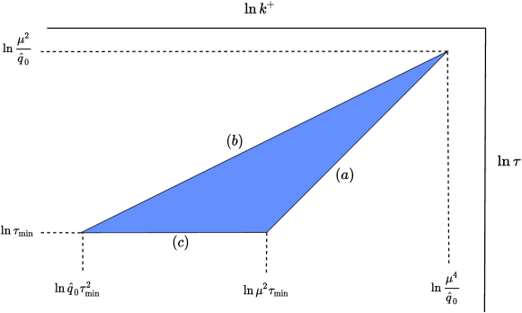
Figure 2: Schematic depiction of the bounds on the integral in Eq. (5). The $(b)$ side of the triangle is given by $\tau=\sqrt{k^{+}/\hat{q}_{0}}$ whereas the $(a)$ one is given by $\tau=k^{+}/\mu^{2}$. The logarithmic axes allow one to easily read the result of the integral Eq. (5) straight from the figure, up to the prefactor $\alpha_{s}C_{R}\hat{q}_{0}/\pi$. Our labeling for the three boundaries follows that of Liou:2013qya .

We now specify the integration limits keeping us in the single scattering regime. Moreover, instead of integrating over $k_{\perp}$, it will be more convenient to integrate over the formation time of the radiated gluon, $\tau\equiv k^{+}/k_{\perp}^{2}$. The limits, which we show in Fig. 2, are then Liou:2013qya

• $\tau<\sqrt{k^{+}/\hat{q}_{0}}$, represented by line $(b)$ in Fig. 2. In the deep Landau–Pomeranchuk–Migdal (LPM) multiple scattering regime, $k_{\perp}^{2}\sim\hat{q}_{0}\tau$. The former constraint then emerges upon demanding that $\tau<k_{\perp}^{2}/\hat{q}_{0}$ and solving for $\tau$. Effectively, this prevents the formation time from getting sufficiently large to lead us into the multiple scattering regime, which will cut off the double-logarithmic phase space: the collinear $dk_{\perp}^{2}/k_{\perp}^{2}$ log can exist as long as the initial and final states can propagate along straight lines for sufficiently long times before and after the single scattering Arnold:2008zu .

• $\tau>k^{+}/\mu^{2}$, represented by line $(a)$. This condition on the formation time corresponds to enforcing the UV cutoff on transverse momentum, i.e. $k_{\perp}<\mu$. In the original derivation of Liou:2013qya this $\mu$ cutoff is identified with $Q_{s}^{2}\equiv\hat{q}L_{\mathrm{med}}$. If instead $\mu>Q_{s}$ the boundaries of the double-logarithmic region change, as shown in Blaizot:2019muz .

• $\tau>\tau_{\mathrm{min}}$, represented by line $(c)$. This IR cutoff $\tau_{\mathrm{min}}$ is intended to render the end result finite. The motivation for this boundary comes from requiring that the duration of the single scattering does not become comparable to the formation time of the radiated gluon, as the former is treated as instantaneous within the collinear-radiation framework. In Liou:2013qya ; Blaizot:2013vha this duration was assumed to be proportional to the inverse temperature, leading to $\tau_{\mathrm{min}}\sim 1/T$. We return to this assumption in the next section.

This leads us to

$$\delta\hat{q}_{\text{\cite[cite]{\@@bibref{Authors Phrase1YearPhrase2}{Liou:2013qya,Blaizot:2013vha}{\@@citephrase{(}}{\@@citephrase{)}}}}}(\mu)=\frac{\alpha_{s}C_{R}}{\pi}\hat{q}_{0}\int_{\tau_{\mathrm{min}}}^{\mu^{2}/\hat{q}_{0}}\frac{d\tau}{\tau}\int_{\hat{q}_{0}\tau^{2}}^{\mu^{2}\tau}\frac{dk^{+}}{k^{+}},$$ (5)

from which the double-logarithmic correction,

$$\delta\hat{q}_{\text{\cite[cite]{\@@bibref{Authors Phrase1YearPhrase2}{Liou:2013qya,Blaizot:2013vha}{\@@citephrase{(}}{\@@citephrase{)}}}}}(\mu)=\frac{\alpha_{s}C_{R}}{2\pi}\hat{q}_{0}\ln^{2}\frac{\mu^{2}}{\hat{q}_{0}\tau_{\mathrm{min}}}$$ (6)

immediately follows. This is the form of Blaizot:2013vha ; that of Liou:2013qya arises by choosing $\mu^{2}=\hat{q}_{0}L_{\mathrm{med}}$, so that the argument of the double logarithm becomes the familiar $L_{\mathrm{med}}/\tau_{\mathrm{min}}$. The single-logarithmic corrections arising from a more sophisticated analysis of the regions neighboring the three boundaries of the triangle shown in Fig. 2 have been presented in Liou:2013qya .

3 Thermal scales in the double-logarithmic phase space

The double-logarithmic phase space we just sketched, as per Liou:2013qya ; Blaizot:2013vha , is derived for a medium described by a random color field with a non-zero two-point function for the $A^{-}$ component, i.e.

$$\left\langle A^{-a}(\bm{q}_{\perp},x^{+})A^{-b}(\bm{q}_{\perp}^{\prime},x^{+^{\prime}})\right\rangle=\delta^{ab}\delta(x^{+}-x^{+^{\prime}})n(x^{+})(2\pi)^{2}\delta^{(2)}(\bm{q}_{\perp}-\bm{q}_{\perp}^{\prime})\frac{g^{4}}{q_{\perp}^{4}}$$ (7)

This corresponds for instance to the time-honored parametrisation of a medium of static scattering centres of density $n$. However, a weakly-coupled QGP contains more medium effects than those captured by these instantaneous, space-like interactions; in particular, as soon as the light-cone frequency ($k^{+}$) range overlaps with the temperature scale, one needs to account for the Bose–Einstein stimulated emission of the radiated gluon and, at negative $k^{+}$, for the absorption of a gluon from the medium. We could naively account for these effects by amending Eq. (5) into

$$\delta\hat{q}(\mu)=\frac{\alpha_{s}C_{R}}{\pi}\hat{q}_{0}\int_{\tau_{\mathrm{min}}}^{\mu^{2}/\hat{q}_{0}}\frac{d\tau}{\tau}\int_{\hat{q}_{0}\tau^{2}}^{\mu^{2}\tau}\frac{dk^{+}}{k^{+}}\left(1+2n_{\mathrm{B}}(k^{+})\right),$$ (8)

where $n_{\mathrm{B}}(k^{+})\equiv(e^{\frac{k^{+}}{T}}-1)^{-1}$ is the Bose-Einstein distribution. Its factor of two in Eq. (8) accounts for stimulated emission and for absorption, which has been reflected in the positive-frequency range.

The smallest frequency in Eq. (8) and in the corresponding original triangle of Fig. 2 is $\hat{q}_{0}\tau_{\mathrm{min}}^{2}$. To completely exclude the $k^{+}\sim T$ range and thus make the thermal contribution exponentially small, one should then require $\tau_{\mathrm{min}}\gg\sqrt{T/\hat{q}_{0}}\sim 1/(g^{2}T)$. Would this be consistent with a single-scattering picture? To answer this, let us recall a few relevant timescales in weakly-coupled QGPs. Scattering processes exchanging $k_{\perp}^{2}$ happen at a rate — see e.g. Arnold:2007pg ; Arnold:2008zu

$$\Gamma_{k_{\perp}^{2}}\sim\frac{g^{4}T^{3}}{\max(k_{\perp}^{2},m_{D}^{2})},\quad\text{for}\;k_{\perp}\gtrsim g^{2}T.$$ (9)

This arises from the $k_{\perp}^{-4}$ form of $\mathcal{C}(k_{\perp})$. We have not shown the Coulomb logarithm of $k_{\perp}^{2}$ over $m_{D}^{2}$, with $m_{D}\sim gT$ the Debye (chromoelectric) screening mass — see Eq. (50). This also means that a $k_{\perp}^{2}\gg(gT)^{2}$ amount may be accumulated either through a rarer hard scattering or through multiple softer ones.

We further recall that the duration of a scattering process is $\mathcal{O}(k_{\perp}^{-1})$. Hence, for the rarer scatterings with $k_{\perp}\sim T$ the duration is indeed $\mathcal{O}(1/T)$, as per Liou:2013qya ; Blaizot:2013vha , whereas for the more frequent soft scatterings the duration is longer by $1/g$, so that in principle more care is needed in drawing and approaching the $\tau\gtrsim\tau_{\mathrm{min}}$ boundary of the phase space — line $(c)$ in Fig. 2 — in a weakly-coupled QGP.

In addition to this latest consideration, $1/g^{2}T$ is the mean free time between the frequent soft, $k_{\perp}\sim gT$ scatterings with the medium constituents. The dipole factor in Eq. (2) is complemented in a thermal QGP by thermal masses of order $gT$ and by the resummation of these frequent soft scatterings on this $1/g^{2}T$ timescale Arnold:2001ba ; Arnold:2002ja . This suppresses the impact of the non-perturbative ultrasoft scatterings and makes it so that $\tau\gtrsim 1/g^{2}T$ for the multiple scattering regime, thus answering negatively our previous question. In more detail, if we look at the LPM estimate $\tau\sim\sqrt{k^{+}/\hat{q}_{0}}$, we have that $\tau\sim(g^{2}T)^{-1}$ for $k^{+}\sim T$ and that it grows for growing $k^{+}$. In other words, for $k^{+}\sim T$ only scatterings with $k_{\perp}\sim gT$ have to be resummed in the multiple scattering regime, whereas for $k^{+}\gg T$ multiple soft scatterings and a single harder scattering can both occur within this parametrically longer formation time, giving rise in turn to a logarithmic enhancement that justifies the HO approximation. We recommend the pedagogical discussion in Arnold:2008zu for further clarifications.

We also note that, for frequencies parametrically smaller than the temperature, which $\tau_{\mathrm{min}}\sim 1/T$ allows ($\hat{q}/T^{2}\sim g^{4}T$), we then have $\sqrt{k^{+}/\hat{q}_{0}}<1/g^{2}T$; this boundary $(b)$ too becomes ill-defined there. Furthermore, the factorisation into soft and collinear logarithms undergirding Eq. (5) is predicated on a collinear expansion $k^{+}\gg k_{\perp}$, i.e. $\tau k^{+}\gg 1$ Iancu:2014kga . This $\ln\tau>-\ln k^{+}$ line in principle excludes parts of Fig. 2: the $(b)-(c)$ vertex is below it, since $\hat{q}\tau_{\mathrm{min}}^{3}\sim g^{4}\ll 1$ for $\tau_{\mathrm{min}}\sim 1/T$. The exclusion stretches to the $\ln\tau=-\ln k^{+}$ line, which crosses lines $(c)$ and $(b)$ if $\mu\tau_{\mathrm{min}}>1$, i.e. $\mu>T$. If instead $\mu<T$ it crosses lines $(a)$ and $(b)$.

Where and how does the thermal distribution contribute to Eq. (8)? How should we address the duration-dependent formation time boundary? How should we make sense of the deep LPM boundary $(b)$ if $k^{+}\ll T$ and of the collinearity boundary $\tau k^{+}>1$? And finally, how does the transition to the classical corrections studied in CaronHuot:2008ni take place? As the $\tau k^{+}>1$ discussion suggests, the answer turns out to depend on the magnitude of $\mu$ compared to the temperature. We start by discussing the case $\mu<T$. The discussion of this section is limited to the double-logarithmic correction in the HO approximation, though some of our more technical results, as presented in the subsequent sections, pave the way for a treatment beyond this accuracy.

3.1 Double logarithms for $\mu<T$

How can we address the issues we just outlined? A naive way out would be to require $\tau_{\mathrm{min}}\gg 1/(g^{2}T)$, as depicted by the upper triangle in Fig. 3, which we have thus purposefully colored in the same shade as the original triangle in Fig. 2: in this region $k^{+}\gg T$ and the $n_{\mathrm{B}}$-proportional thermal contribution to Eq. (8) is exponentially small. However, as was previously noted, this large $\tau_{\mathrm{min}}$ would amount to only considering radiative processes with a long formation time, at odds with the $\tau\ll 1/(g^{2}T)$ requirement for a strict single soft scattering regime. Furthermore, as we shall explain, our detailed evaluation of the strict single scattering regime with $\tau\ll 1/(g^{2}T)$, $k^{+}\sim T$ finds a double-log-enhanced contribution there. We thus conclude that $\tau_{\mathrm{min}}$ cannot be larger than $1/g^{2}T$; for strict single scatterings to be included, we must have $\tau_{\mathrm{min}}\ll 1/(g^{2}T)$. If line $(b)$ were to be taken seriously at $k^{+}<T$, we would thus be including parts of the thermal and subthermal frequency range.

Moreover, our position is that the “single-scattering” definition employed in the literature on double logs is not exclusively that of a strict single scattering: the collinear divergence gets cut off when $k_{\perp}$ becomes small enough ($\tau$ large enough) that multiple scatterings start to contribute within a formation time, and that this happens before entering the so-called “deep LPM” regime $k_{\perp}^{2}\sim\hat{q}_{0}\tau$. However, at double-logarithmic accuracy we do not (in fact, we cannot) distinguish between a $k_{\perp}^{2}\gg\hat{q}_{0}\tau$ and a $k_{\perp}^{2}\sim\hat{q}_{0}\tau$ boundary, and in the HO approximation — see the discussion above and footnote 3 — we cannot disentangle multiple soft scatterings from a single harder one. As mentioned, the analysis of Liou:2013qya deals with single-logarithmic corrections to this boundary within the HO approximation; in Sec. 5, we shall show how that boundary can be investigated in the future beyond that approximation.

Our strategy is thus the following: we introduce an intermediate regulator $\tau_{\mathrm{int}}$, with $1/gT\ll\tau_{\mathrm{int}}\ll 1/g^{2}T$. The lower boundary will be discussed soon, whereas the upper boundary makes it so that for $\tau>\tau_{\mathrm{int}}$ we thus include parts of the strict single scattering regime, as well as the “few scatterings” regime just mentioned. This region is then given by

$$\delta\hat{q}(\mu)^{\mathrm{few}}=\frac{\alpha_{s}C_{R}}{\pi}\hat{q}_{0}\int_{\tau_{\mathrm{int}}}^{\mu^{2}/\hat{q}_{0}}\frac{d\tau}{\tau}\int_{\hat{q}_{0}\tau^{2}}^{\mu^{2}\tau}\frac{dk^{+}}{k^{+}}\left(1+2n_{\mathrm{B}}(k^{+})\right).$$ (10)

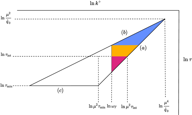
Figure 3: A pictorial representation of how the phase space of the radiated gluon is partitioned once thermal effects are taken into account. See the main text for the explanation of the different subregions.

Graphically, it is represented in Fig. 3 by the triangle above $\tau=\tau_{\mathrm{int}}$, which corresponds to the 1 and 2 subregions. We have filled the 1 region in blue for $\tau\gtrsim 1/g^{2}T$, where the effect of the thermal distributions is irrelevant, and in ochre for $\tau_{\mathrm{int}}<\tau<1/g^{2}T$, where they start to contribute. For reasons that will become clear shortly, the smaller 2 triangle has not been shaded. Indeed, as we shall show in App. C.1, the double-logarithmic terms from the integration of Eq. (10) are

$$\delta\hat{q}(\mu)_{\mathrm{dlog}}^{\mathrm{few}}=\frac{\alpha_{s}C_{R}}{2\pi}\hat{q}_{0}\bigg{\{}\ln^{2}\frac{\mu^{2}}{\hat{q}_{0}\tau_{\mathrm{int}}}-\frac{1}{2}\ln^{2}\frac{\omega_{T}}{\hat{q}_{0}\tau_{\mathrm{int}}^{2}}\bigg{\}}\quad\text{with}\;\omega_{T}=\frac{2\pi T}{e^{\gamma_{E}}}\quad\text{for}\;\;\frac{\omega_{T}}{\mu^{2}}\ll\tau_{\mathrm{int}}\ll\sqrt{\frac{\omega_{T}}{\hat{q}_{0}}}.$$ (11)

Here $\gamma_{E}$ is the Euler–Mascheroni constant and $\omega_{T}$ is the $\mathcal{O}(T)$ scale which naturally appears once thermal are effects into account. While its precise value can only be determined from the integration, its scaling could be expected and is related to the vacuum-thermal cancellation we shall discuss soon. Graphically, if we take $k^{+}=\omega_{T}$ as a vertical line in Fig. 3, the first term in Eq. (11) comes from integrating over the entire “1+2” triangle, whereas the second term comes from subtracting the smaller 2 triangle, which therefore does not contribute to double-logarithmic accuracy. Furthermore, this $k^{+}=\omega_{T}$ line intersects line $(b)$ at $\sqrt{\omega_{T}/\hat{q}_{0}}\sim 1/g^{2}T$, thus excluding the range where the formation time estimate becomes unreliable.

We also remark that, for $\tau_{\mathrm{int}}>\tau_{\mathrm{min}}$, the horizontal $\tau=\tau_{\mathrm{int}}$ line intersects the diagonal sides of the triangle at $k^{+}=\hat{q}_{0}\tau_{\mathrm{int}}^{2}$ (line $(b)$) and $k^{+}=\mu^{2}\tau_{\mathrm{int}}$ (line $(a)$). The form (11) arises when the temperature scale $\omega_{T}$ falls in between these two values, so that $\hat{q}_{0}\tau_{\mathrm{int}}^{2}\ll\omega_{T}\ll\mu^{2}\tau_{\mathrm{int}}$, resulting in the range of validity expressed there. This is where the size of $\mu$ with respect to the medium scales enters. At leading order, i.e. without considering these radiative corrections, choosing $gT\ll\mu\ll T$ ensures that only the contributions of the soft modes Aurenche:2002pd are included, whereas $T\ll\mu$ also includes the thermal-mode contribution Arnold:2008vd . If we allow for radiative corrections and further require a strict single-scattering contribution, we shall show that $\mu\gg\sqrt{g}T$ is necessary, so as to include the so-called semi-collinear processes of Ghiglieri:2013gia ; Ghiglieri:2015ala . Finally, $\frac{\omega_{T}}{\mu^{2}}\ll\tau_{\mathrm{int}}$ should be complemented by the duration bound $\tau_{\mathrm{int}}\gg\tau_{\mathrm{min}}$: for $\mu\ll T$ this is automatically satisfied, whereas for $\mu\gtrsim T$ it will then be a further constraint to be imposed. In other words, for $\mu<\sqrt{\omega_{T}/\tau_{\mathrm{min}}}\sim T$ the vertical $k^{+}=\omega_{T}$ line intersects boundaries $(b)$ and $(a)$, whereas for $\mu>\sqrt{\omega_{T}/\tau_{\mathrm{min}}}\sim T$ it would intersect $(b)$ and $(c)$.

For formation times below $\tau_{\mathrm{int}}$, the process happens in the strict single scattering regime. It also becomes sensitive to the fact that, over parts of that range, the duration of the strict single scattering, as per our previous discussion, is parametrically of the same order of the formation time. This happens because the region includes soft $l_{\perp}\sim gT$ scatterings whose duration overlaps with formation times of order $1/gT$, which are part of this region — hence our $\tau_{\mathrm{int}}\gg 1/gT$ requirement. As we shall show in Sec. 4, our evaluation, based on these semi-collinear processes, naturally accounts for these finite-duration effects, removing the need for a hard cutoff $\tau>\tau_{\mathrm{min}}$. This corresponds to the regions 3 and 4 in Fig. 3. As we mentioned, it also gives rise to a double-logarithmic correction. It turns out that, to double-logarithmic accuracy in the HO approximation, our result corresponds to the area of the magenta 3 region — we return to this fact soon. It can thus be directly read off from Fig. 3 as

$$\delta\hat{q}(\mu)^{\text{single}}_{\mathrm{dlog}}=\delta\hat{q}(\mu)^{\text{(3)}}_{\mathrm{dlog}}=\frac{\alpha_{s}C_{R}}{2\pi}\hat{q}_{0}\ln^{2}\frac{\mu^{2}\tau_{\mathrm{int}}}{\omega_{T}}.$$ (12)

Upon summing Eqs. (11) and (12) we then find

$$\delta\hat{q}(\mu)_{\mathrm{dlog}}=\delta\hat{q}(\mu)_{\mathrm{dlog}}^{\mathrm{few}}+\delta\hat{q}(\mu)^{\text{single}}_{\mathrm{dlog}}=\frac{\alpha_{s}C_{R}}{4\pi}\hat{q}_{0}(\rho\ll\mu)\ln^{2}\frac{\mu^{4}}{\hat{q}_{0}\omega_{T}}.$$ (13)

We thus see that in this formula, which is one of our main results, $\tau_{\mathrm{min}}$ has disappeared: it has been replaced with the scale $\omega_{T}$. The dependence on the intermediate cutoff $\tau_{\mathrm{int}}$ has also vanished. We have further specified that the scale $\rho$ of $\hat{q}_{0}$ needs to be smaller than that of $\delta\hat{q}$, in keeping with the $l_{\perp}\ll k_{\perp}$ expansion undergirding Eq. (4). Since $\mu\ll T$ here, the expression to be used is then Eq. (55). Eq. (13) also justifies a posteriori — see footnote 5 — that the first range of $k_{\perp}$ giving rise to a double-logarithmic enhancement is $k_{\perp}\sim\sqrt{g}T$, $\mu>\sqrt{g}T$: had we chosen $k_{\perp}\sim gT$ the argument of the double log in Eq. (13) would have been of order one.

Upon imposing $\mu^{2}=\hat{q}_{0}L_{\mathrm{med}}$, as in Liou:2013qya , Eq. (13) becomes

$$\delta\hat{q}(\sqrt{\hat{q}_{0}L_{\mathrm{med}}})_{\mathrm{dlog}}=\frac{\alpha_{s}C_{R}}{4\pi}\hat{q}_{0}\ln^{2}\frac{\omega_{c}}{\omega_{T}},$$ (14)

where $\omega_{c}=\hat{q}_{0}L^{2}$ is the maximal frequency for medium-induced radiation Baier:1996kr . This formula is however only valid for $1/g^{3}T\ll L_{\mathrm{med}}\ll 1/g^{4}T$, that is for media thicker than a soft mean free path but thinner that a large-angle scattering mean free path.

We further remark that the effect of a populated medium can be understood, to double-logarithmic accuracy, as replacing the horizontal $\tau>\tau_{\mathrm{min}}$ line with a vertical $k^{+}>\omega_{T}\sim T$ line: up to our usual prefactor of $\alpha_{s}C_{R}\hat{q}_{0}/\pi$, $1/4\ln^{2}(\mu^{4}/\hat{q}_{0}\omega_{T})$ is precisely the area of the “1+3” shaded triangle in Fig. 3. Since lines $k^{+}=\omega_{T}$ and $(a)$ intersect at $\tau=\omega_{T}/\mu^{2}$, this shaded triangle is entirely above the collinearity bound $\tau k^{+}>1$.

The physical picture behind the emergence of the $\omega_{T}$ scale is that for $k^{+}\gg T$ the thermal part $n_{\mathrm{B}}(k^{+})$ of the phase space factor $1/2+n_{\mathrm{B}}(k^{+})$ is exponentially small, whereas for $k^{+}<T$, the vacuum part — $1/2$ — cancels against the first quantum correction coming from the expanded $n_{\mathrm{B}}(k^{+})$, i.e.

$$n_{\mathrm{B}}(k^{+}\ll T)=\frac{T}{k^{+}}-\frac{1}{2}+\mathcal{O}\left(\frac{k^{+}}{T}\right).$$ (15)

Hence, the logarithmic part of the integral is unaffected in the UV, but it is no longer cut off in the IR by the boundary of the integration — $\hat{q}_{0}\tau_{\mathrm{min}}^{2}$ — but rather by a quantity of order $T$, whose precise value $\omega_{T}$ emerges as a property of the integral in Eq. (8). This can be better seen from the following simpler single-logarithmic integral, with $\nu_{\mbox{\tiny IR}}\ll T\ll\nu_{\mbox{\tiny UV}}$

$$\int^{\nu_{\mbox{\tiny UV}}}_{\nu_{\mbox{\tiny IR}}}\frac{dk^{+}}{k^{+}}\Big{(}\underbrace{1}_{\mathrm{vacuum}}+\underbrace{2n_{\mathrm{B}}(k^{+})}_{\mathrm{thermal}}\Big{)} =\underbrace{\ln\frac{\nu_{\mbox{\tiny UV}}}{\nu_{\mbox{\tiny IR}}}}_{\mathrm{vacuum}}\;+\underbrace{\frac{2T}{\nu_{\mbox{\tiny IR}}}-\ln\frac{2\pi T}{\nu_{\mbox{\tiny IR}}e^{\gamma_{E}}}+\mathcal{O}\left(\frac{\nu_{\mbox{\tiny IR}}}{T},\exp(-\nu_{\mbox{\tiny UV}}/T)\right)}_{\mathrm{thermal}}$$

$$=\frac{2T}{\nu_{\mbox{\tiny IR}}}+\ln\frac{\nu_{\mbox{\tiny UV}}e^{\gamma_{E}}}{2\pi T}+\mathcal{O}\left(\frac{\nu_{\mbox{\tiny IR}}}{T},\exp(-\nu_{\mbox{\tiny UV}}/T)\right)\,.$$ (16)

More details on the evaluation are provided in App. C.1.

The attentive reader will have noticed that this cancellation does not affect the classical $T/k^{+}$ term, which is the largest in the IR, though it is not logarithmically divergent. Instead this term will yield a contribution that is proportional to power laws of $\mu$ and $\tau_{\mathrm{min}}$; in the example just shown, this would be the $T/\nu_{\mbox{\tiny IR}}$ term. Power-law terms are in general not physical: they just represent a non-logarithmic sensitivity to a neighboring region and must, for IR-safe quantities like $\hat{q}$, cancel with opposite power laws from said region. In our case, this neighboring region is the one where both $L$ and $K$ are soft. In that region, the diagrams in Fig. 1 are part of the calculation of Caron-Huot CaronHuot:2008ni . In terms of Fig. 3, this region has overlap with the “4” and “5” trapezoids. As we shall show in detail in Sec. 4 and App. C.3, these classical power law terms cancel against those coming from power-law corrections to the calculation of CaronHuot:2008ni that we shall derive. This undoubtedly shows in a non-trivial way how the classical and quantum regions are connected.

In summary, for $\sqrt{g}T<\mu<T$ — at double-logarithmic accuracy we can use the $\ll$ and $<$ delimiters interchangeably — our main result is that the shape of the double-logarithmic phase space changes from that of Fig. 2 to the shaded “1+3” one of Fig. 3: the horizontal line $(c)$, $\tau>\tau_{\mathrm{min}}\sim 1/T$, gets replaced by a vertical line $k^{+}>\omega_{T}\sim T$. The fact that the more sophisticated evaluation of the semi-collinear region, to be presented in Sec. 4, together with the regulated evaluation above the intermediate cutoff $\tau_{\mathrm{int}}$, reproduces this simple form signals that effects analyzed in the semi-collinear evaluation, such as the necessary relaxation of the instantaneous approximation, are not relevant at double-logarithmic accuracy in the HO approximation, as we shall show there.

3.2 Extension to $\mu>T$

Up until this point, we have taken $T\gg\mu\gg\sqrt{g}T$, the first range where double-logarithm corrections appear. We now move on to consider what happens if $\mu\gg T$ in terms of the structure of the relevant portion of phase space. If we start from Fig. 3 and proceed to increase $\mu$, line $(a)$ gets shifted to the right, making the original $(a)-(b)-(c)$ triangle larger. As we argued previously, once $\mu>\sqrt{\omega_{T}/\tau_{\mathrm{min}}}\sim T$ the vertical $k^{+}=\omega_{T}$ line intersects lines $(b)$ and $(c)$ rather than $(b)$ and $(a)$. Hence, nothing would change for the part of the evaluation for $\tau>\tau_{\mathrm{int}}$, as given by Eq. (11). On the other hand, the evaluation of the strict single scattering regime, for $\tau<\tau_{\mathrm{int}}$, needs to be amended to account for this. It must also account for the fact that for $\mu\gtrsim T$ we are thus including strict single scatterings where $l_{\perp}$ is approaching or possibly exceeding the $T$ scale. In principle one would thus need to account for the fact that the coefficient of the leading-log (harmonic-oscillator) $\hat{q}_{0}$ is not constant. As shown in Arnold:2008vd and summarized in App. B, $\hat{q}_{0}(\rho\ll T)$ and $\hat{q}_{0}(\rho\gg T)$ differ at leading-log by 15% for $N_{f}=3$ and $N_{c}=3$, so in a first approximation we may neglect this effect. We leave a more precise evaluation of semi-collinear processes in this region to future work.

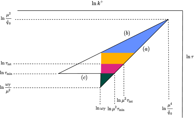
Figure 4: Structure of phase space once the cutoff on $\mu$ is allowed to increase to values much larger than the temperature. Notably, region “6” in dark green emerges. It cannot be well described by our setup due to the associated small formation time.

Under this approximation, we can simply extend Eq. (12) to the present case. This would however include the dark green triangle “6” in Fig. 4, which lies under the $\tau=\tau_{\mathrm{min}}$ line. It is not clear whether this sharp line needs to be included, and only an evaluation like the one we show in detail in the next section, but extended to larger $\mu$ can address the effect of the relaxation of the instantaneous approximation in this setting. The expectation from the previous $\mu<T$ results is that this effect should be subleading. We however choose to proceed conservatively here and subtract that slice from our result. Moreover, parts of this triangle lie below the $\tau k^{+}=1$ line, further motivating its subtraction. In our double-logarithmic approximation this corresponds again, for the reasons just explained in the previous subsection, to subtracting off the area of that triangle. This leads to

$$\delta\hat{q}(\mu\gg T)_{\mathrm{dlog}} =\frac{\alpha_{s}C_{R}}{2\pi}\hat{q}_{0}(\rho\ll\mu)\left[\frac{1}{2}\ln^{2}\left(\frac{\mu^{4}}{\hat{q}_{0}\omega_{T}}\right)-\ln^{2}\left(\frac{\mu^{2}\tau_{\mathrm{min}}}{\omega_{T}}\right)\right]$$

$$=\frac{\alpha_{s}C_{R}}{2\pi}\hat{q}_{0}(\rho\ll\mu)\left[\ln^{2}\left(\frac{\mu^{2}}{\hat{q}_{0}\tau_{\mathrm{min}}}\right)-\frac{1}{2}\ln^{2}\left(\frac{\omega_{T}}{\hat{q}_{0}\tau_{\mathrm{min}}^{2}}\right)\right].$$ (17)

Unsurprisingly, the subtraction of the “6” triangle from the “1+3+6” triangle on the first line is equal to that of the unshaded “2+5” triangle from the original $(a)-(b)-(c)$ triangle on the second line. This implies that, for $\mu>T$, our result is closer to the original one of Liou:2013qya . This can be better appreciated by noting that the vertical line at $k^{+}=\mu^{2}\tau_{\mathrm{min}}$ cuts the $(a)-(b)-(c)$ triangle into two triangles of equal area. Hence, for $\omega_{T}>\mu^{2}\tau_{\mathrm{min}}$, i.e. $\mu\lesssim T$ our result (13) is less than half of the original double logarithm (6), whereas for $\mu>\sqrt{\omega_{T}/\tau_{\mathrm{min}}}$ our result (17) is more than half of it.

4 Single scattering for $\tau<1/g^{2}T$, $k^{+}\gtrsim T$

Our previous section presented all our main results to double-logarithmic accuracy forgoing detail for the sake of a concise and self-contained explanation. In particular, we left out the detailed evaluation of our main computational result of this paper: the determination of the strict single scattering contribution for $\tau<\tau_{\mathrm{int}}$ and the connection to the soft, classical contribution. We now provide both. In Sec. 4.1 we describe the general computational setup, in 4.2 we introduce semi-collinear processes and derive the double-log contribution. In Sec. 4.3 we discuss the interplay with the classical region and in Sec. 4.4 we analyze subleading contributions.

4.1 Computational setup

The natural computational setup for a calculation of transverse momentum broadening — not dissimilar from that of Liou:2013qya — is to consider a Wilson loop in the $(x^{+},x_{\perp})$ plane — see App. A for our conventions — through which we can define the scattering rate and $\hat{q}$ CasalderreySolana:2007qw ; CaronHuot:2008ni ; DEramo:2010ak ; Benzke:2012sz . The Wilson loop reads, taking a quark source for illustration

$$\langle W(x_{\perp})\rangle=\frac{1}{N_{c}}\mathrm{Tr}\langle[0,x_{\perp}]_{-}\mathcal{W}^{\dagger}(x_{\perp})[x_{\perp},0]_{+}\mathcal{W}(0)\rangle,$$ (18)

where the Wilson lines read

$$\mathcal{W}(x_{\perp})=\mathcal{P}\exp\Big(ig\int_{-\frac{L_{\mathrm{med}}}{2}}^{\frac{L_{\mathrm{med}}}{2}}dx^{+}A^{-}(x^{+},x_{\perp})\Big{missing}),$$ (19)

and

$$[x_{\perp},y_{\perp}]_{\pm}=\mathcal{P}\exp\Big(-ig\int_{1}^{0}ds(y_{\perp}-x_{\perp})\cdot A_{\perp}(\pm\frac{L_{\mathrm{med}}}{2},x_{\perp}+(y_{\perp}-x_{\perp})s)\Big{missing}).$$ (20)

The fields in this Wilson loop are to be understood as transforming in the representation of the parton and as path-ordered, so that one can think (in non-singular gauges) of $\mathcal{W}$ as the eikonalized jet quark in the amplitude and $\mathcal{W}^{\dagger}$ as its conjugate-amplitude counterpart.

Exponentiation dictates that

$$\lim_{L_{\mathrm{med}}\to\infty}\langle W(x_{\perp})\rangle=\exp(-\mathcal{C}(x_{\perp})L_{\mathrm{med}}),$$ (21)

which we can use, together with

$$\mathcal{C}(x_{\perp})=\int\frac{d^{2}k_{\perp}}{(2\pi)^{2}}(1-e^{i\bm{x}_{\perp}\cdot\bm{k}_{\perp}})\mathcal{C}(k_{\perp}),$$ (22)

to recover $\mathcal{C}(k_{\perp})$. In a non-singular gauge — we shall adopt later on in App. D the strict Coulomb gauge — the $[\ldots,\ldots]_{\pm}$ Wilson lines do not contribute to $\mathcal{C}(x_{\perp})$. Eq. (22) further shows how $x_{\perp}$-independent diagrams — those with no gluon exchange between the two $\mathcal{W}$ — will not contribute to $\mathcal{C}(x_{\perp})$ and thus to $\hat{q}$; they only contribute to probability conservation by reducing the probability of acquiring no transverse momentum.

4.2 Semi-collinear processes

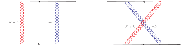
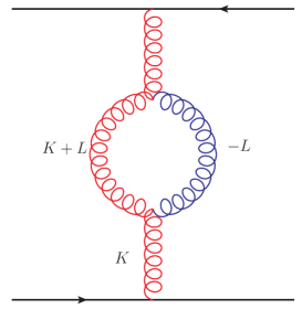
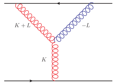
Figure 5: Diagrams giving rise to the single-scattering regime. The two horizontal solid lines are the Wilson lines $\mathcal{W}$. Red gluons are coft, blue ones are HTL-resummed and soft, see main text. Momenta flow bottom to top.

Let $P=(p^{+},p^{-},p_{\perp})=E(1,0,0)$, with $E\gg T$, be the momentum of the hard jet parton. Then a mode $Q\sim E(1,\lambda^{2},\lambda)$, with $\lambda\ll 1$ an expansion parameter, is a collinear mode. DEramo:2010ak ; Benzke:2012sz argued that such modes are not included in this Wilson loop setup. Radiative corrections like those we are after are on the other hand included in this Wilson loop framework: the emitted gluon is collinear, but it carries a momentum fraction $k^{+}+l^{+}\approx k^{+}\ll E$. Borrowing the terminology of Becher:2015hka , we call these modes coft, with $Q\sim\lambda^{\prime}E(1,\lambda^{2},\lambda)$, $\lambda,\lambda^{\prime}\ll 1$. The single-scattering processes then arise, in the region we are interested in, from the interaction of these modes with HTL-resummed soft modes. We portray the relevant diagrams in Fig. 5.

As the two $\mathcal{W}$ lines represent the hard jet parton in the amplitude and conjugate amplitude, a cut is understood to go horizontally through the middle of each diagram. It then follows that the first two diagrams in Fig. 5 corresponds to the square of the first two in Fig. 1 and their interference. The third diagram here corresponds to the square of the third there. Finally the fourth here corresponds to the interference of the first two with the third there.

So in principle we are presented with the evaluation of these diagrams in the specific scaling $k_{\perp}\sim\sqrt{g}T\gg l_{\perp}\sim gT$, $k^{+}\sim T$ that is responsible for the double log in the strict scattering regime for $\mu<T$. This detailed calculation will be presented in App. D, together with the discussion of the virtual counterpart to the processes shown in Fig. 1, confirming that they do not represent a double-logarithmic effect, as per Liou:2013qya . This Wilson-loop based determination will thus confirm how these radiative corrections are also encoded in that object, thus paving the way for our later contact with the UV boundaries of the soft NLO calculation of Caron-Huot CaronHuot:2008ni , which also used the Wilson loop setup.

Here we instead present a more intuitive derivation, drawing from the literature. Namely, $k_{\perp}\sim\sqrt{gT}\gg l_{\perp}\sim gT$, $k^{+}\sim T$ is the semi-collinear region identified in Ghiglieri:2013gia ; Ghiglieri:2015ala . There it was found that it is precisely this semi-collinear process that happens on a shorter formation time $\tau_{\mathrm{semi}}\sim 1/(gT)$ than the strictly collinear one $\tau_{\mathrm{coll}}\gtrsim 1/(g^{2}T)$ through a single scattering with the medium. The one single scattering exchanges $l_{\perp}\sim gT$; its duration is thus of the same order of $\tau_{\mathrm{semi}}$, causing the breakdown of the instantaneous approximation. Thus, addressing this corresponds to “crossing” boundary $(c)$, in the language of Liou:2013qya .

The evaluation of Ghiglieri:2013gia ; Ghiglieri:2015ala addressed this non-instantaneous nature. In more detail, the strict collinear regime corresponds, in the momentum labeling of Fig. 1, to $l^{-}\approx(\bm{k}_{\perp}+\bm{l}_{\perp})^{2}/(2k^{+})\sim g^{2}T\ll l^{+},l_{\perp}\sim gT$, as arising from the on-shell conditions for the outgoing $K+L$ and $P-K$ legs. Thus, when Fourier-transforming the $L$ propagator to position space one can neglect its $l^{-}$ dependence, leading to instantaneous propagation in the $x^{+}$ direction. Conversely, in the semi-collinear regime $k_{\perp}\sim\sqrt{g}T,k^{+}\sim T$, so that $l^{-}\approx k_{\perp}^{2}/(2k^{+})\sim gT\sim l^{+},l_{\perp}\sim gT$. Hence the outgoing gluon has the scaling $(K+L)\sim T(1,gT,\sqrt{g}T)$, which is what was identified in Ghiglieri:2013gia ; Ghiglieri:2015ala as semi-collinear. In our language it represents a specific coft scaling, as per Footnote 7. In this scaling $l^{-}$ is no longer negligible with respect to $l^{+}$ and $l_{\perp}$, so that the $L$ gluon exchange is no longer instantaneous in $x^{+}$. In momentum space, this no longer restricts $L$ to space-like values, thus opening the phase space for the absorption and emission of soft, time-like plasmons, as shown in the example in Fig. 6.

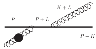
Figure 6: One of the extra diagrams that appear once the duration of the jet-medium interaction is comparable to the gluon formation time. The blob represents a resummed Hard Thermal Loop: the $L$ gluon is thus a time-like plasmon. Diagrams corresponding to the other processes of Fig. 1, as well as the plasmon emission/gluon absorption crossings are not shown.

We can then directly take the results of Ghiglieri:2015ala , which computed these semi-collinear processes in the non-abelian case. By inspecting Fig. 10 of Ghiglieri:2015ala one arrives at the dictionary $K_{\text{\cite[cite]{\@@bibref{Authors Phrase1YearPhrase2}{Ghiglieri:2015ala}{\@@citephrase{(}}{\@@citephrase{)}}}}}\to L$, $Q_{\text{\cite[cite]{\@@bibref{Authors Phrase1YearPhrase2}{Ghiglieri:2015ala}{\@@citephrase{(}}{\@@citephrase{)}}}}}\to K$. The derivation of Ghiglieri:2013gia ; Ghiglieri:2015ala lead to an integrated-in-transverse momentum rate; however, in intermediate steps a consistent labeling of momenta was maintained in all diagrams, so that this integration can be undone naturally. We can then take Eq. (8.8) of Ghiglieri:2015ala , undo the transverse integration, apply the dictionary and take the soft-gluon limit $x\to 0$ in the $q\to qg$ and $g\to gg$ processes, together with a $p\to\infty$ one for consistency. This leads to

$$(2\pi)^{2}\frac{d\Gamma_{\mathrm{semi}}}{dk^{+}d^{2}k_{\perp}}=\frac{g^{2}C_{R}}{\pi k^{+}k_{\perp}^{4}}(1+n_{\mathrm{B}}(k^{+}))\hat{q}\left(\rho;\frac{k_{\perp}^{2}}{2k^{+}}\right),$$ (23)

whence — see Eq. (1)

$$\delta\mathcal{C}(k_{\perp})_{\mathrm{semi}}=\frac{g^{2}C_{R}}{\pi k_{\perp}^{4}}\int\frac{dk^{+}}{k^{+}}(1+n_{\mathrm{B}}(k^{+}))\hat{q}\left(\rho;\frac{k_{\perp}^{2}}{2k^{+}}\right).$$ (24)

$\hat{q}(\rho;k_{\perp}^{2}/2k^{+})$ is a modified (adjoint) $\hat{q}$ that also accounts for the $l^{-}$-dependence, i.e.

$$\hat{q}(\rho;l^{-})=g^{2}C_{A}T\int^{\rho}\frac{d^{2}l_{\perp}}{(2\pi)^{2}}\left[\frac{m_{D}^{2}l_{\perp}^{2}}{(l_{\perp}^{2}+l^{-2})(l_{\perp}^{2}+l^{-2}+m_{D}^{2})}+2\frac{l^{-2}}{l_{\perp}^{2}+l^{-2}}\right].$$ (25)

In the $l^{-}\ll gT$ limit it reduces to the soft contribution to $\hat{q}_{0}(\rho)$ Aurenche:2002pd in Eq. (55), and thus Eq. (24) reduces, up to the statistical factor, to Eq. (3). With respect to Eq. (8.8) of Ghiglieri:2015ala we have also undone the subtractions performed there, which were meant to isolate the strictly semi-collinear process from its collinear and harder limits, so as to avoid double countings. Something similar needs to happen here: elastic $2\leftrightarrow 2$ scatterings exchanging $k_{\perp}\gg gT$ are the hard contribution to $\hat{q}$, as in Arnold:2008vd . As we show in detail in App. C.2, the integration over the leading-order phase space does include the region where $\sqrt{g}T\lesssim k_{\perp}\lesssim T$ and either the incoming or outgoing gluon from the medium ($L$ here) becomes soft, $L\sim gT$. As that calculation treats this gluon with bare propagators, it does not properly account for its soft dynamics, as encoded by HTL resummation. Hence, the semi-collinear limit of the calculation of Arnold:2008vd must be subtracted from Eq. (25), to avoid double counting it. This yields

$$\hat{q}(\rho;l^{-})_{\mathrm{subtr}}\equiv\hat{q}(\rho;l^{-})-\hat{q}(\rho;l^{-})_{\text{\cite[cite]{\@@bibref{Authors Phrase1YearPhrase2}{Arnold:2008vd}{\@@citephrase{(}}{\@@citephrase{)}}}}}=g^{2}C_{A}T\int^{\rho}\frac{d^{2}l_{\perp}}{(2\pi)^{2}}\frac{m_{D}^{2}l_{\perp}^{2}}{(l_{\perp}^{2}+l^{-2})(l_{\perp}^{2}+l^{-2}+m_{D}^{2})},$$ (26)

i.e. it removes the second term of Eq. (25), precisely as found in Ghiglieri:2013gia ; Ghiglieri:2015ala .

Eq. (26), when plugged in Eq. (24), is UV log-divergent for $\rho\gg l^{-},m_{D}$. This is not unexpected, as Eq. (24) is obtained under the assumption that $l_{\perp}\ll k_{\perp}$. We can thus set $\rho\ll k_{\perp}\ll\mu$, leading to

$$\hat{q}(\rho;l^{-})_{\mathrm{subtr}}=\alpha_{s}C_{A}T\bigg{\{}\underbrace{m_{D}^{2}\ln\left(\frac{\rho^{2}}{m_{D}^{2}}\right)}_{\mathrm{HO}}\;\underbrace{-l^{-2}\ln\left(1+\frac{m_{D}^{2}}{l^{-2}}\right)-m_{D}^{2}\ln\left(1+\frac{l^{-2}}{m_{D}^{2}}\right)}_{l^{-}-\mathrm{dependent}}\bigg{\}}.$$ (27)

Our labeling in the underbraces emphasizes that the first, $l^{-}$-independent term is precisely Eq. (55), the harmonic-oscillator approximation to $\hat{q}_{0}(\rho)$ for $gT\ll\rho\ll T$. In our adoption of the HO approximation, we may for the moment treat $\rho$ as a parameter. If we were to go beyond it, we would have to complement the evaluation here with the neighboring region, where $k_{\perp}\sim l_{\perp}\gg gT$. That scaling includes both a single harder scattering and a multiple scattering contribution, which arises when $|k_{\perp}+l_{\perp}|$ becomes small, causing the formation time to become long. Addressing these processes properly requires dealing with LPM resummation beyond the HO approximation: we discuss this outlook in Sec. 5.

Hence, the effect of our more sophisticated approach, which relaxes the instantaneous approximation, is only contained in the $l^{-}$-dependent terms in Eq. (27). The HO term is instead identical to what would have arisen directly from the simpler evaluation of Sec. 3. Its contribution to $\hat{q}$ is thus

$$\delta\hat{q}_{\mathrm{semi}}^{\mathrm{HO}}=4\alpha_{s}C_{R}\hat{q}_{0}(\rho)\int\frac{d^{2}k_{\perp}}{(2\pi)^{2}}\frac{1}{k_{\perp}^{2}}\int\frac{dk^{+}}{k^{+}}(1+n_{\mathrm{B}}(k^{+})),$$ (28)

We can evaluate this expression by once again keeping only the even part of the frequency integrand and adding a factor of $2$ to account for the negative frequency range. We can change variables to $\tau=k^{+}/k_{\perp}^{2}=1/(2l^{-})$ and enforce the boundaries $\tau_{\mathrm{int}}>\tau>k^{+}/\mu^{2}$, which are respectively the intermediate regulator and line $(a)$ of Sec. 3. We further introduce an IR regulator for the frequency, $k^{+}>k^{+}_{\mbox{\tiny IR}}$, with $T\gg k^{+}_{\mbox{\tiny IR}}\gg gT$, so as to avoid the soft frequency regime of CaronHuot:2008ni . This then implies $k^{+}<\mu^{2}\tau_{\mathrm{int}}$, i.e.

$$\delta\hat{q}_{\mathrm{semi}}^{\mathrm{HO}}=\frac{\alpha_{s}C_{R}}{\pi}\hat{q}_{0}(\rho)\int_{k^{+}_{\mbox{\tiny IR}}}^{\mu^{2}\tau_{\mathrm{int}}}\frac{dk^{+}}{k^{+}}\left(1+2n_{\mathrm{B}}(k^{+})\right)\int_{k^{+}/\mu^{2}}^{\tau_{\mathrm{int}}}\frac{d\tau}{\tau}.$$ (29)

As we shall see, the $k^{+}_{\mbox{\tiny IR}}$ regulator only affects power law terms, but not double-logarithmic ones, because of the vacuum-thermal cancellation discussed in Sec. 3. As we show in more detail in App. C.1, the integrations yield

$$\delta\hat{q}_{\mathrm{semi}}^{\mathrm{HO}}=\frac{\alpha_{s}C_{R}}{2\pi}\hat{q}_{0}(\rho)\bigg{[}\frac{4T\ln\left(\frac{\mu^{2}\tau_{\mathrm{int}}}{k^{+}_{\mbox{\tiny IR}}e}\right)}{k^{+}_{\mbox{\tiny IR}}}+\left(\ln^{2}\left(\frac{\mu^{2}\tau_{\mathrm{int}}}{\omega_{T}}\right)-2\gamma_{1}+\frac{\pi^{2}}{4}-\gamma_{E}^{2}\right)\bigg{]}+\mathcal{O}\left(k^{+}_{\mbox{\tiny IR}},e^{-\mu\tau_{\mathrm{int}}^{2}/T}\right),$$ (30)

where $\gamma_{n}$ is the nth Stieltjes constant and $\omega_{T}=2\pi Te^{-\gamma_{E}}$. The double-logarithmic term is precisely the one anticipated in Eq. (12). Here we show the accompanying constant and the $T/k^{+}_{\mbox{\tiny IR}}$ power-law divergence, which signals the overlap with the soft, classical region.

4.3 Connection to the classical contribution

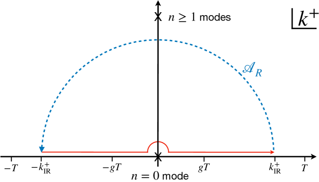
Figure 7: The contour discussed in the main text for the evaluation of the retarded part of the soft contribution to Eq. (31). The corresponding advanced part is not shown. The cross at the origin is Matsubara zero mode, hence the deformation of the (red) integration contour there, which gives rise to the Euclidean contribution.

How does this $T/k^{+}_{\mbox{\tiny IR}}$ dependence cancel with the soft, classical region? Diagrams such as those in Fig. 5 are precisely those evaluated in CaronHuot:2008ni with $K\sim L\sim gT$. Hence, on that side the calculation must present a $1/k^{+}_{\mbox{\tiny IR}}$ term, where now $k^{+}_{\mbox{\tiny IR}}$ is a UV cutoff that can thus be safely sent to infinity. Indeed, no such term appears in the expression of CaronHuot:2008ni . Furthermore, no $k^{+}$ integration appears either: as we mentioned, the classical-mode contribution can be mapped to the 3D Euclidean theory — see CaronHuot:2008ni for the original derivation and Ghiglieri:2015zma for a more pedagogical review. Let us look for illustration at the tree-level one-gluon exchange

$$\mathcal{C}(x_{\perp})=g^{2}C_{R}\int\frac{d^{4}K}{(2\pi)^{4}}(1-e^{i\bm{k}_{\perp}\cdot\bm{x}_{\perp}})\left(\frac{1}{2}+n_{\mathrm{B}}(k^{0})\right)(G^{--}_{R}(K)-G^{--}_{A}(K))2\pi\delta(k^{-}),$$ (31)

where the $\delta(k^{-})$ comes from the Wilson-line integrations at large $L_{\mathrm{med}}$ and $G_{R}$ ($G_{A}$) is the retarded (advanced) gluon propagator. The key observation is that causality dictates that $G_{R}$ ($G_{A}$) is analytical in the upper (lower) half $k^{+}$ plane, so that the only poles are those in the statistical function, at $k^{0}=k^{+}=in2\pi T$, $n\in\mathbb{Z}$. In principle we can then close the contour at infinite $k^{+}$ and pick up the residues of all these poles. However, for $x_{\perp}\gg 1/T$ the zero mode dominates, yielding the mapping to EQCD. This corresponds to having replaced $1/2+n_{\mathrm{B}}(k^{+})$ with $T/k^{+}$ and closed the contour on an arc $\mathcal{A}_{R}$ between the zeroth and first Matsubara modes, as shown in Fig. 7. If we identify the radius of this arc with $k^{+}_{\mbox{\tiny IR}}$ (indeed $gT\ll k^{+}_{\mbox{\tiny IR}}\ll T$), we may take it as large, if we look at things from the soft side of the calculation. Hence, any function that falls to zero faster than $1/k^{+}$ on this arc will only give rise to inverse powers of $k^{+}_{\mbox{\tiny IR}}$, which could then safely be neglected in the derivation of CaronHuot:2008ni . This is indeed the case both for the LO and NLO soft contributions — the LO case can be checked by plugging in Eq. (31) the HTL-resummed Coulomb-gauge propagators given in Eqs. (48) and (LABEL:htltrans). In App. C.3 we show that Ghiglieri:2015ala computed diagrams related to those in Fig. 5, expanded precisely on that $\mathcal{A}_{R}$ arc. Starting from these results we show how the arc terms precisely cancel the $T/k^{+}_{\mbox{\tiny IR}}$ ones in Eq. (30).

We have thus shown how the IR slice of the double-logarithmic phase space overlaps with that of the soft contributions determined in CaronHuot:2008ni . In fact, CaronHuot:2008ni already commented on the possible sensitivity to collinear modes (coft in our language) at relative order $g^{2}$ and how they would show up, on the soft side, as a failure of the $T/k^{+}$ classical approximation to the Bose–Einstein distribution. Our findings thus confirm in detail this general expectation.

4.4 Subleading contributions

We now turn to the remainder of Eq. (27). The $l^{-}$-dependent terms, integrated with the same boundaries as in Eq. (28), give rise to — see again App. C.1

$$\delta\hat{q}_{\mathrm{semi}}^{l^{-}-\mathrm{dep}}=-\frac{\alpha_{s}^{2}C_{R}C_{A}Tm_{D}^{2}}{3\pi}\left[\ln^{3}\frac{e^{1/2}\mu^{2}}{2\omega_{T}m_{D}}+\mathcal{O}\left(\frac{T}{k^{+}_{\mbox{\tiny IR}}},\ln,\mathrm{const}\right)\right].$$ (32)

We are not showing explicitly single-logarithmic terms and constants, which are included in Eq. (70). Neither do we show the divergent power-law terms, proportional to $T/k^{+}$, which will again cancel against classical contributions. We also do not show other power laws in the other cutoffs, as they can be similarly argued to cancel against neighboring regions.

We remark that the leading term in Eq. (32) is a triple logarithm of $\mu^{2}/(m_{D}\omega_{T})$. It is thus independent of $\tau_{\mathrm{int}}$ and could then be directly added to Eq. (13). We argue that Eq. (32) is smaller than Eq. (13): the latter, reinstating the log of $\hat{q}_{0}(\rho)$, is $\propto\ln(\rho^{2}/m_{D}^{2})\ln^{2}(\mu^{2}/\sqrt{\hat{q}_{0}\omega_{T}})$. $\mu^{2}/\sqrt{\hat{q}_{0}\omega_{T}}$ is larger by $1/g$ than $\mu^{2}/(m_{D}\omega_{T})$, which is instead comparable to $\rho^{2}/m_{D}^{2}$, since $\rho\ll\mu$. Hence Eq. (32) represents a subleading correction; it is the first to feature a logarithmic dependence on the soft screening scale. This is somewhat analogous to what was found in Liou:2013qya when crossing line $(c)$ — and thus relaxing the instantaneous approximation — for a nuclear medium: it still generated a term with the highest number of logarithms, but with a smaller argument in some of them.

If we wanted to extend the present calculation to larger values of $\mu$, so as to deal more precisely with region “6” of Fig. 4, we would need to understand how $\hat{q}(\rho;l^{-})$ changes once $\rho$ starts to include the thermal range: this corresponds to the generalisation to non-zero $l^{-}$ of the connection between the $l_{\perp}\sim gT$ and $l_{\perp}\sim T$ regimes discussed in App. B. Let us finally point out that the subleading triple-log in Eq. (32) is negative and that, for moderate values of the coupling $g$, may overtake the leading term in Eq. (13). And more generally, the determinations at the highest logarithmic order (LL) are numerically not precise until the first (NLL) corrections are determined — see for instance Arnold:2008zu for the splitting rate in the deep LPM regime and Arnold:2003zc for transport coefficients. Eq. (32) is only a part of the subleading corrections to the double-log in Eq. (13): in the next section we present a pathway to a more precise determination of boundary $(b)$.

5 Transverse momentum broadening beyond the harmonic oscillator

Up until this point we have, with the exception of Sec. 4.4, only discussed double-logarithmic corrections, and only done so within the harmonic-oscillator approximation. Thus, we had to infer the coefficient of the HO $\hat{q}_{0}$ from other considerations, i.e. the single-scattering requirement $\rho\ll\mu$. We also explained in Sec. 3 how, within these two approximations, we cannot distinguish the region where few scatterings are contributing from the deep LPM regime where many scatterings are contributing. Hence, the boundary $(b)$ had to be imposed by hand whenever relevant, giving rise to the $\hat{q}_{0}$ dependence in the argument of the double logarithm in Eq. (13). In this section we now present, as an outlook, a way to proceed beyond these two approximations and self-consistently determine boundary $(b)$.

To this end, we will thus derive, starting from the formalism of Liou:2013qya ; Iancu:2014kga , an LPM resummation equation that is not restricted to the harmonic-oscillator approximation. By numerically solving that equation and performing the integrations over the two logarithmic variables $k^{+}$ and $\tau$ (or equivalently $k^{+}$ and $k_{\perp}$) one would then see the emergence of multiple scatterings cutting off the double-log and thus be able to determine how good of an approximation line $(b)$ is. Let us then start from Eqs. (6), (7), (11) and (12) in Liou:2013qya (see also (55)), which construct a framework for resumming multiple interactions in the HO approximation and in the large-$N_{c}$ limit. Combining (11) and (12) yields, in the notation of Liou:2013qya

$$S(x_{\perp})=-\alpha_{s}C_{R}\mathrm{Re} \int\frac{d\omega}{\omega^{3}}\int_{0}^{L_{\mathrm{med}}}dz_{2}\int_{0}^{z_{2}}dz_{1}\nabla_{\bm{B}_{2\perp}}\cdot\nabla_{\bm{B}_{1\perp}}$$

$$\times\bigg{[}e^{-\hat{q}_{p}x_{\perp}^{2}(L_{\mathrm{med}}-z_{2}+z_{1})/4}G_{\mathrm{HO}}(\bm{B}_{2\perp},z_{2};\bm{B}_{1\perp},z_{1})-\mathrm{vac}\bigg{]}\bigg{|}^{\bm{B}_{2\perp}=\bm{x}_{\perp}}_{\bm{B}_{2\perp}=0}\bigg{|}^{\bm{B}_{1\perp}=\bm{x}_{\perp}}_{\bm{B}_{1\perp}=0},$$ (33)

where we have already undone the large-$N_{c}$ approximation by replacing $N_{c}/2$, the original large-$N_{c}$ limit of $C_{F}$, with $C_{R}$. $\hat{q}_{p}$, with $p=q,g$ denotes the specific partonic broadening coefficients for a quark or gluon source. The $d\omega$ frequency integration is understood over the positive frequencies of the radiated gluon. The propagator $G_{\mathrm{HO}}$ is the Green’s function of the following Schrödinger equation (see (55) there)

$$\bigg{\{}i\partial_{z}+\frac{\nabla^{2}_{B_{\perp}}}{2\omega}+\frac{i}{4}\bigg{[}\hat{q}_{p}x_{\perp}^{2}+\frac{\hat{q}_{g}}{2}\big{(}B_{\perp}^{2}+(\bm{B}_{\perp}-\bm{x}_{\perp})^{2}-x_{\perp}^{2}\big{)}\bigg{]}\bigg{\}}G_{\mathrm{HO}}(\bm{B}_{\perp},z;\bm{B}_{1\perp},z_{1})=0,$$ (34)

with

$$G_{\mathrm{HO}}(\bm{B}_{\perp},z_{1};\bm{B}_{1\perp},z_{1})=\delta^{(2)}(\bm{B}_{\perp}-\bm{B}_{1\perp}).$$ (35)

“vac” denotes the subtraction of the vacuum term $G_{0}$, i.e. the solution of Eq. (39) with a vanishing $\hat{q}$. The double vertical bars at the end of Eq. (33) signify that the expression in brackets should be understood as

$$e^{-\frac{\hat{q}_{p}x_{\perp}^{2}}{4}(L_{\mathrm{med}}-z_{2}+z_{1})}\bigg{[} G_{\mathrm{HO}}(\bm{x}_{\perp},z_{2};\bm{x}_{\perp},z_{1})+G_{\mathrm{HO}}(0,z_{2};0,z_{1})$$

$$-G_{\mathrm{HO}}(\bm{x}_{\perp},z_{2};0,z_{1})-G_{\mathrm{HO}}(0,z_{2};\bm{x}_{\perp},z_{1})\bigg{]}-\mathrm{vac}.$$ (36)

Physically, these four terms can be understood as the two positive, virtual terms, where the gluon is emitted and reabsorbed within the amplitude (both $\bm{B}_{\perp}=0$) or conjugate amplitude (both $\bm{B}_{\perp}=\bm{x}_{\perp}$) minus the real terms, where the gluon is emitted on one side and absorbed on the other side of the cut.

As a first step, we can identify their $S$-matrix element with our $\langle W(x_{\perp})\rangle$. Hence we can equate

$$S(x_{\perp})=\exp[-L_{\mathrm{med}}(\mathcal{C}(x_{\perp})+\delta\mathcal{C}(x_{\perp}))]\approx e^{-L_{\mathrm{med}}\mathcal{C}(x_{\perp})}(1-L_{\mathrm{med}}\delta\mathcal{C}(x_{\perp})).$$ (37)

Secondly, Eq. (33) is in the harmonic-oscillator approximation, i.e.

$$\mathcal{C}_{p}(x_{\perp})\stackrel{{\scriptstyle\mathrm{HO}}}{{=}}\frac{\hat{q}_{p}}{4}x_{\perp}^{2},$$ (38)

We can then undo this approximation, so that Eq. (34) becomes

$$\bigg{\{}i\partial_{z}+\frac{\nabla^{2}_{B_{\perp}}-m_{\infty\,g}^{2}}{2\omega}+i\bigg{[}\mathcal{C}_{p}(x_{\perp})+\frac{1}{2}\big{(}\mathcal{C}_{g}(B_{\perp})+\mathcal{C}_{g}(|\bm{B}_{\perp}-\bm{x}_{\perp}|)-\mathcal{C}_{g}(x_{\perp})\big{)}\bigg{]}\bigg{\}}G(\bm{B}_{\perp},z;\bm{B}_{1\perp},z_{1})=0,$$ (39)

where we have also introduced the gluon’s asymptotic mass, with $m_{\infty\,g}^{2}=m_{D}^{2}/2$ at leading order — see CaronHuot:2008uw for the NLO determination and Moore:2020wvy ; Ghiglieri:2021bom for non-perturbative contributions.

Let us comment that the form of Eq. (39) decomposes the three-body scattering kernel (the hard jet parton in the amplitude and conjugate amplitude and the radiated gluon) into three two-body kernels with different color assignments. Perturbatively this is valid up to, and including, the $\mathcal{O}(g)$ NLO corrections, as discussed in CaronHuot:2008ni . The long-distance, non-perturbative behaviour of this three-pole object is at present unknown. For a leading-order determination of radiative correction from this formalism, it should suffice to use the smooth kernel provided by the Fourier transform of Eq. (53) as $\mathcal{C}_{q}$ and $\mathcal{C}_{g}$ in Eq. (39). We refer to Ghiglieri:2018ltw ; Moore:2021jwe for details on this numerical transform.

Finally, we can also account for the effect of a populated medium by considering the effects of stimulated emission and absorption, i.e $\int d\omega\theta(\omega)\to\int dk^{+}(1/2+n_{\mathrm{B}}(k^{+}))$ where we have replaced $\omega$ with $k^{+}$, in keeping with our notation. In a longitudinally uniform medium $G$ is only a function of $\tau\equiv z_{2}-z_{1}$, so that we can use our identification (37) to obtain, in the large-$L_{\mathrm{med}}$ limit

$$\delta\mathcal{C}(x_{\perp})=\alpha_{s}C_{R}\mathrm{Re}\int\frac{dk^{+}}{k^{+3}}\left(\frac{1}{2}+n_{\mathrm{B}}(k^{+})\right)\int_{0}^{L_{\mathrm{med}}}d\tau\,\nabla_{\bm{B}_{2\perp}}\cdot\nabla_{\bm{B}_{1\perp}}\bigg{[} e^{\mathcal{C}_{p}(x_{\perp})\tau}G(\bm{B}_{2\perp},\bm{B}_{1\perp};\tau)$$

$$-\mathrm{vac}\bigg{]}\bigg{|}^{\bm{B}_{2\perp}=\bm{x}_{\perp}}_{\bm{B}_{2\perp}=0}\bigg{|}^{\bm{B}_{1\perp}=\bm{x}_{\perp}}_{\bm{B}_{1\perp}=0}.$$ (40)

We observe that the source-specific part of the scattering kernel in the Hamiltonian (39) and the amplification factor $e^{\mathcal{C}_{p}(x_{\perp})\tau}$ can be eliminated by noting that if $\tilde{G}(\bm{B}_{\perp},\bm{B}_{1\perp};\tau)\equiv e^{\mathcal{C}_{p}(x_{\perp})\tau}G(\bm{B}_{\perp},\bm{B}_{1\perp};\tau)$ is a Green’s function of the operator

$$\bigg{\{}i\partial_{\tau}+\frac{\nabla^{2}_{B_{\perp}}-m_{\infty\,g}^{2}}{2k^{+}}+\frac{i}{2}\big{(}\mathcal{C}_{g}(B_{\perp})+\mathcal{C}_{g}(|\bm{B}_{\perp}-\bm{x}_{\perp}|)-\mathcal{C}_{g}(x_{\perp})\big{)}\bigg{\}}\tilde{G}(\bm{B}_{\perp},\bm{B}_{1\perp};\tau)=0,$$ (41)

then $G(\bm{B}_{\perp},\bm{B}_{1\perp};\tau)$ is a Green’s function of Eq. (39). Hence

$$\delta\mathcal{C}(x_{\perp})=\alpha_{s}C_{R}\mathrm{Re}\int\frac{dk^{+}}{k^{+3}}\left(\frac{1}{2}+n_{\mathrm{B}}(k^{+})\right)\int_{0}^{L_{\mathrm{med}}}d\tau\,\nabla_{\bm{B}_{2\perp}}\cdot\nabla_{\bm{B}_{1\perp}}\bigg{[} \tilde{G}(\bm{B}_{2\perp},\bm{B}_{1\perp};\tau)$$

$$-\mathrm{vac}\bigg{]}\bigg{|}^{\bm{B}_{2\perp}=\bm{x}_{\perp}}_{\bm{B}_{2\perp}=0}\bigg{|}^{\bm{B}_{1\perp}=\bm{x}_{\perp}}_{\bm{B}_{1\perp}=0}.$$ (42)

This reformulation makes transparent the fact that the Hamiltonian only contains the purely non-abelian $\mathcal{C}_{g}$. That is because, before or after both emission vertices, there are only the two source lines for the hard jet parton and one-gluon exchanges between them are resummed into $\exp\big(-\mathcal{C}_{p}(x_{\perp})(L_{\mathrm{med}}-\tau)\big{missing})$. In the time region between the two emission vertices, the hard jet parton and conjugate hard jet parton lines are no longer a color singlet, with corresponding color factor $C_{R}$, but rather an octet, with color factor $C_{R}-C_{A}/2$. This corresponds to the $\mathcal{C}_{p}(x_{\perp})-\mathcal{C}_{g}(x_{\perp})/2$ combination in Eq. (39). But we should remove the overall $\exp\big(-\mathcal{C}_{p}(x_{\perp})L_{\mathrm{med}}\big{missing})$ damping, as per our dictionary (37), which, thanks to our manipulation in Eq. (41), leads to the outright disappearance of the $\mathcal{C}_{p}(x_{\perp})$ part, corresponding to the fact that those exchanges would happen also in the absence of the radiated gluon. Up to the statistical factors and thermal masses, Eqs. (41) and  (42) agree with Iancu:2014kga .

Finally, for a medium that is isotropic in the azimuthal direction we can use the reflection symmetry $\bm{B}_{\perp}\to\bm{x}_{\perp}-\bm{B}_{\perp}$ of Eq. (41) to simplify Eq. (42) into

$$\delta\mathcal{C}(x_{\perp})=2\alpha_{s}C_{R}\mathrm{Re}\int\frac{dk^{+}}{k^{+3}}\left(\frac{1}{2}+n_{\mathrm{B}}(k^{+})\right)\int_{0}^{L_{\mathrm{med}}}d\tau\,\nabla_{\bm{B}_{2\perp}}\cdot\nabla_{\bm{B}_{1\perp}}\bigg{[} \tilde{G}(\bm{B}_{2\perp},\bm{B}_{1\perp};\tau)$$

$$-\mathrm{vac}\bigg{]}\bigg{|}^{\bm{B}_{2\perp}=\bm{x}_{\perp},\bm{B}_{1\perp}=0}_{\bm{B}_{2\perp}=0,\bm{B}_{1\perp}=0}.$$ (43)

Eq. (41) is, together with Eq. (43), the main result of this section. As we anticipated, its solution would allow a much better understanding of how the double logarithm is cut off by the transition from single to multiple scatterings as a function of the energy $k^{+}$ of the radiated gluon. Furthermore, Eq. (41) goes beyond the HO which we had to introduce in Eq. (27); as we remarked there, regions where $\bm{l}_{\perp}+\bm{k}_{\perp}$ becomes small would become sensitive to multiple scatterings, which are correctly addressed here. However, Eq. (41) is not easy to solve, as it would require generalizing the methods of CaronHuot:2010bp ; Andres:2020vxs ; Andres:2020kfg ; Schlichting:2021idr to the extra dependence on $x_{\perp}$ of $\tilde{G}$. As a first step, one could consider using the improved opacity expansion introduced in Mehtar-Tani:2019ygg ; Barata:2020rdn ; Barata:2021wuf ; Isaksen:2022pkj to capture the qualitative aspects of the transition from the HO approximation to including rarer harder scatterings.

We shall leave the full or approximate solution of Eq. (41) to future work. We conclude this section by providing a non-trivial consistency check, namely that the single-scattering term in Eqs. (41) and (43) agrees with the standard results in the single-scattering regime. That follows by taking the Fourier transforms of Eqs. (41) and Eq. (43), i.e. starting from

$$\tilde{G}(\bm{B}_{2\perp},\bm{B}_{1\perp};\tau)\equiv\int\frac{d^{2}p_{\perp}}{(2\pi)^{2}}\int\frac{d^{2}q_{\perp}}{(2\pi)^{2}}e^{i\bm{B}_{2\perp}\cdot\bm{p}_{\perp}}e^{-i\bm{B}_{1\perp}\cdot\bm{q}_{\perp}}\tilde{G}(\bm{p}_{\perp},\bm{q}_{\perp};\tau).$$ (44)

Upon using the method of CaronHuot:2010bp it is possible to obtain the $N=1$ contribution through a tedious calculation, yielding, in the large-$L_{\mathrm{med}}$ limit

$$\delta\mathcal{C}(x_{\perp})^{N=1}=2\alpha_{s}C_{R}\int\frac{dk^{+}}{k^{+}} \left(1+2n_{\mathrm{B}}(k^{+})\right)\int\frac{d^{2}p_{\perp}}{(2\pi)^{2}}\int\frac{d^{2}l_{\perp}}{(2\pi)^{2}}\,\mathcal{C}_{g}(l_{\perp})\frac{(1-e^{i\bm{x}_{\perp}\cdot\bm{p}_{\perp}})(1+e^{i\bm{x}_{\perp}\cdot\bm{l}_{\perp}})}{p_{\perp}^{2}+m_{\infty\,g}^{2}}$$

$$\times\bigg{[}\frac{p_{\perp}^{2}}{p_{\perp}^{2}+m_{\infty\,g}^{2}}-\frac{\bm{p}_{\perp}\cdot(\bm{p}_{\perp}+\bm{l}_{\perp})}{(\bm{p}_{\perp}+\bm{l}_{\perp})^{2}+m_{\infty\,g}^{2}}\bigg{]}.$$ (45)

At this point we need to extract the real-process contribution, $\delta\mathcal{C}(k_{\perp})^{\mathrm{real}}_{\mathrm{single}}$. This just corresponds to Fourier-transforming $\bm{x}_{\perp}$ into $\bm{k}_{\perp}$ and only keeping terms proportional to $\exp(i\bm{x}_{\perp}\cdot\bm{p}_{\perp})$ and $\exp(i\bm{x}_{\perp}\cdot(\bm{p}_{\perp}+\bm{l}_{\perp}))$, yielding

$$\delta\mathcal{C}(k_{\perp})^{\mathrm{real}}_{\mathrm{single}}= 4\alpha_{s}C_{R}\int dk^{+}\frac{\frac{1}{2}+n_{\mathrm{B}}(k^{+})}{k^{+}}\int\frac{d^{2}l_{\perp}}{(2\pi)^{2}}\mathcal{C}_{g}(l_{\perp})\left[\frac{\bm{k}_{\perp}}{k_{\perp}^{2}+m_{\infty\,g}^{2}}-\frac{\bm{k}_{\perp}+\bm{l}_{\perp}}{(\bm{k}_{\perp}{+}\bm{l}_{\perp})^{2}+m_{\infty\,g}^{2}}\right]^{2}.$$ (46)

In the $m_{\infty\,g}\to 0$ limit and neglecting the thermal distribution ($1/2+n_{\mathrm{B}}(k^{+})\to\theta(k^{+})$) this agrees with Eq. (2). The $x_{\perp}$-independent term in $\delta\mathcal{C}(x_{\perp})^{N=1}$ is the usual probability-conserving contribution, whereas the term proportional to $\exp(i\bm{x}_{\perp}\cdot\bm{l}_{\perp})$ encodes virtual processes. In App. D.2 we show its explicit form and prove that it agrees with our direct diagrammatic evaluation.

6 Conclusions and outlook

In this paper we have analyzed double-log enhanced quantum corrections to transverse momentum broadening in a weakly-coupled QGP. These corrections arise from the recoil in transverse momentum after a medium-induced radiation is sourced by a single scattering with the medium. The region of phase space for the double logarithm, as represented in Fig. 2, was shown in Liou:2013qya ; Blaizot:2013vha to be triangular in logarithmic units of formation time $\tau$ and frequency $k^{+}$ of the radiated gluon, resulting in Eq. (6). We show that the boundary of said region is only valid in media whose sole effect is to provide transverse-momentum kicks to the propagating hard jet parton.

In our case, on the other hand, the thermal population of dynamical gluons changes the shape of the phase space, since the original triangle necessarily overlaps with regions where $k^{+}$ is order $T$ or smaller. There one needs to account for Bose-stimulated emission and for absorption of thermal gluons from the bath. This results in Figs. 3 and 4, which are the main results of this paper, together with the associated Eqs. (13) and (17). What these figures and equations show is that thermal emission and absorption change the infrared limits of the double-logarithmic integral: no frequencies smaller than $\mathcal{O}(T)$ contribute to these double logs. This low-frequency region corresponds to the unshaded, white areas in both figures: only the colored regions to the right of the vertical $k^{+}=\omega_{T}=2\pi Te^{-\gamma_{E}}$ line contribute to the double logs. This is then reflected in the two equations: at double-logarithmic accuracy, the area of the shaded regions corresponds to the radiative correction.

How does this happen? We show that the effect of thermal absorption and emission is described by changing the $dk^{+}/k^{+}$ logarithmic frequency integral into $dk^{+}/k^{+}(1+2n_{\mathrm{B}}(k^{+}))$, with $n_{\mathrm{B}}$ the thermal distribution. As we explain in Sec. 3.1, as soon as $k^{+}\ll T$, the IR log divergence in the vacuum part cancels with twice the $-1/2$ from the IR expansion of the statistical function, leaving the IR contribution to that integral to be dominated by the non-logarithmic, classical $T/k^{+}$ term in that expansion. In Sec. 4.3 we show in detail how this term smoothly connects radiative quantum corrections to the classical soft corrections determined by Caron-Huot in CaronHuot:2008ni using the mapping to the three-dimensional Euclidean theory he introduced. This is another of our main results: in a weakly-coupled quark-gluon plasma the IR regions of the original double-logarithmic phase space are not $\mathcal{O}(g^{2}\ln^{2})$ quantum corrections but rather part of the $\mathcal{O}(g)$ classical corrections. The vacuum-thermal cancellation of the double-logarithmic piece in these regions naturally separates the two corrections.

It is also worth stressing that our calculation identified two regions that contribute to double-logarithmic radiative corrections: taking Fig. 3 as an example, for the case where the transverse momentum exchange is limited to $\mu\lesssim T$, these are regions “1” and “3”. We have identified “1” as the region where single scatterings start to make way to a regime of “few” scatterings, before eventually reaching the deep LPM, aka “many scattering” regime, represented by line $(b)$, which is expected to cut off the double logarithm. Region “3” is instead restricted to formation times shorter than the mean free time $1/g^{2}T$ between frequent soft scatterings in the medium: it is thus a strict single soft scattering regime, where furthermore the duration of the single scattering overlaps with the formation time. Our treatment in Sec. 4 is based on semi-collinear processes, introduced in Ghiglieri:2013gia ; Ghiglieri:2015ala and properly accounts for these overlapping timescales without resorting to instantaneous approximations. We however find that the leading contribution from this region corresponds to what would emerge from a naive treatment which considers the single scattering instantaneous with respect to the formation time — see Sec. 4.2. The effect arising from the overlapping timescale, as given by Eq. (32), though still logarithmically enhanced, is subleading compared to the former, and represents part of the subleading log corrections that are expected beyond double-logarithmic accuracy.

In Sec. 5 we provide an important ingredient for the determination of radiative corrections beyond this accuracy: we provide a framework — Eqs. (41) and (43) — that can resum multiple scatterings and their LPM interference pattern beyond the harmonic-oscillator approximation, which, like previous literature, we have employed for our previously discussed main results. This is obtained by suitably extending the framework of Liou:2013qya ; Iancu:2014kga . Numerical or semi-analytical solutions of these equations will yield two important advancements: first, they would be able to shed light on how the transition from single to multiple scatterings closes the double-logarithmic phase space at $k^{+}\gg T$, where in a weakly-coupled QGP the mean free time $1/g^{2}T$ between soft scatterings is well separated from the long formation time $\tau\sim\sqrt{k^{+}/\hat{q}_{0}}\sim\sqrt{k^{+}/T}/g^{2}T$. Second, if one wanted to approximate the solution with a double-logarithmic form, these solutions would clarify the $\rho$ scale at which $\hat{q}_{0}$ should be evaluated in the harmonic-oscillator approximation and they would determine subleading single-log corrections from boundary $(b)$. As these solutions are not straightforwardly obtained, we leave these developments to future work.

This also implies that we are currently lacking a consistent determination of all subleading single-log corrections. We feel it would be premature and potentially misleading to assess the quantitative impact of these double-logarithmic corrections: in many cases — see Arnold:2003zc for transport coefficient and Arnold:2008zu for collinear splitting rates — NLL corrections are necessary to have a sensible estimate of the size of LL contributions. The situation is somewhat even more ambiguous in this case, as $\rho$ too is undetermined, as explained.

Our results naturally open other directions for future research: as we discussed in the Introduction, these double- and single-logarithmic radiative correction affect in the same fashion transverse momentum broadening and double gluon emission Blaizot:2014bha ; Wu:2014nca ; Iancu:2014kga ; Arnold:2021mow . Addressing how the emergence of the temperature scale affects double gluon emission would thus be a very interesting natural development.

Finally, resummation equations for the double-log quantum corrections have been derived in Liou:2013qya ; Iancu:2014kga ; Iancu:2014sha and solved in Caucal:2021lgf ; Caucal:2022fhc . These methods are based on the original triangle of Fig. 2 for the double-logarithmic phase space and can be understood as evolving $\hat{q}$ from some initial timescale $\tau_{0}$ to longer timescales by resumming many long-lived quantum fluctuations. A way to incorporate our careful evaluation of the thermal-$k^{+}$ and short-$\tau$ regions could be to use our results below some $\tau_{\mathrm{trans}}\sim 1/g^{2}T$, properly incorporating the vacuum-thermal cancellation as well as our semi-collinear single-scattering regime and, potentially, also the classical regime with its non-perturbative determinations Moore:2019lgw ; Moore:2021jwe ; Schlichting:2021idr . The obtained $\hat{q}(\tau_{\mathrm{trans}})$ could then be passed on as an initial condition to the resummation equations of Caucal:2021lgf ; Caucal:2022fhc , thus naturally factorizing classical and semi-collinear contributions on one side from the quantum evolution on the other. This too is left to future investigations.

Appendix A Conventions

Our sign for the covariant derivative is

$$D_{\mu}=\partial_{\mu}-igA_{\mu},$$

which fixes the sign of the three gluon vertex to be positive. Moreover, we work with the “mostly minus” $(+,-,-,-)$ metric. Uppercase letters denote four-momenta, lowercase letters the modulus of the three-momenta.

We will often be working in light-cone coordinates, where

$$p^{+} \equiv\frac{p^{0}+p^{z}}{2}=\bar{v}_{\mu}p^{\mu},$$

$$p^{-} \equiv p^{0}-p^{z}=v_{\mu}p^{\mu},$$

$$p\cdot q =p^{+}q^{-}+p^{-}q^{+}-\bm{p}_{\perp}\cdot\bm{q}_{\perp},$$

where we have defined the two light-like reference vectors as

$$\bar{v}^{\mu} \equiv\frac{1}{2}(1,0,0,-1),$$

$$v^{\mu} \equiv(1,0,0,1).$$

This asymmetric convention for the ⁺ and ^- components of the light-cone coordinates has two advantages: it has unitary Jacobian, i.e. $dp^{0}dp^{z}=dp^{+}dp^{-}$, and we shall often deal with scalings where $p^{-}\ll p^{+}$, which then implies $p^{0}\approx p^{z}\approx p^{+}$.

Let us now discuss propagators. For convenience we will mostly work in the Keldysh, or $r,a$, basis of the real-time formalism for the computation of thermal expectation values — see Ghiglieri:2020dpq for a review. The two elements of this basis are defined as $\phi_{r}\equiv(\phi_{1}+\phi_{2})/2$, $\phi_{a}\equiv\phi_{1}-\phi_{2}$, $\phi$ being a generic field and the subscripts 1 and 2 labeling the time-ordered and anti-time-ordered branches of the Schwinger-Keldysh contour respectively. The propagator is a $2\times 2$ matrix, where one entry is always zero and only one entry depends on the thermal distribution, i.e.,

$$D=\left(\begin{array}[]{cc}D_{rr}&D_{ra}\\ D_{ar}&D_{aa}\end{array}\right)=\left(\begin{array}[]{ccc}\left(\frac{1}{2}\pm n(p^{0})\right)(D_{R}-D_{A})&&D_{R}\\ D_{A}&&0\end{array}\right),$$ (47)

where $D_{R}$ and $D_{A}$ are the retarded and advanced propagators, the plus (minus) sign refers to bosons (fermions). $n(p^{0})$ is the corresponding thermal distribution, either $n_{\mathrm{B}}(p^{0})=(\exp(p^{0}/T)-1)^{-1}$ for bosons or $n_{\mathrm{F}}(p^{0})=(\exp(p^{0}/T)+1)^{-1}$ for fermions. We also define the spectral function as the difference of the retarded and advanced propagators, $\rho\equiv D_{R}-D_{A}$. We will denote the gluon propagator by $G$.

We will adopt strict Coulomb gauge throughout. The treatment of soft momenta in propagators and vertices requires the use of Hard Thermal Loop (HTL) resummation Braaten:1989mz . Coulomb-gauge HTL-resummed gluons are described by

$$G^{00}_{R}(Q) = \frac{i}{\displaystyle q^{2}+m_{D}^{2}\left(1-\frac{q^{0}}{2q}\ln\frac{q^{0}+q+i\epsilon}{q^{0}-q+i\epsilon}\right)},$$ (48)

$$G^{ij}_{R}(Q) \equiv (\delta^{ij}-\hat{q}^{i}\hat{q}^{j})G^{T}_{R}(Q)=\left.\frac{i(\delta^{ij}-\hat{q}^{i}\hat{q}^{j})}{\displaystyle q_{0}^{2}-q^{2}-m_{\infty}^{2}\left(\frac{q_{0}^{2}}{q^{2}}-\left(\frac{q_{0}^{2}}{q^{2}}-1\right)\frac{q^{0}}{2q}\ln\frac{q^{0}{+}q}{q^{0}{-}q}\right)}\right|_{q^{0}=q^{0}+i\epsilon}.$$

Here

$$m_{D}^{2}=g^{2}T^{2}\left(\frac{N_{c}}{3}+\frac{N_{f}}{6}\right)$$ (50)

is the LO Debye mass and $m_{\infty}^{2}=m_{D}^{2}/2$ is the LO gluon asymptotic mass. The other components of the propagators in the $r,a$ basis can be obtained through Eq. (47).

Appendix B Transverse-momentum broadening kernels

The leading-order transverse momentum broadening kernel comes from elastic $2\leftrightarrow 2$ scatterings with medium constituents. In the soft sector, i.e. $m_{D}\lesssim l_{\perp}\ll T$, these get Landau-damped, leading to Aurenche:2002pd

$$\mathcal{C}(l_{\perp})^{\mathrm{LO}}_{\mathrm{soft}}=\frac{g^{2}C_{R}Tm_{D}^{2}}{l_{\perp}^{2}(l_{\perp}^{2}+m_{D}^{2})}.$$ (51)

For $\sqrt{ET}\gg l_{\perp}\gtrsim T$ one finds Arnold:2008vd

$$\mathcal{C}(l_{\perp})_{\text{hard}}^{\mathrm{LO}}=\frac{g^{4}C_{R}}{l_{\perp}^{4}}\int\frac{d^{3}q}{(2\pi)^{3}}\frac{q-q_{z}}{q}\Big{[}2C_{A}\,n_{\mathrm{B}}(q)(1+n_{\mathrm{B}}(q^{\prime}))+4N_{f}T_{F}\,n_{\mathrm{F}}(q)(1-n_{\mathrm{F}}(q^{\prime}))\Big{]},$$ (52)

where $q^{\prime}=q+\frac{l_{\perp}^{2}+2\bm{l}_{\perp}\cdot\bm{q}}{2(q-q_{z})}$ and $T_{F}=1/2$ for the quark scattering contribution. We refer to Arnold:2008vd for details on the accurate numerical evaluation of this expression. Arnold:2008vd also provided a handy expression that interpolates smoothly between the two regimes by partially resumming higher-order contributions, i.e.

$$\mathcal{C}(l_{\perp})_{\text{smooth}}^{\mathrm{LO}}=\frac{2g^{4}C_{R}}{l_{\perp}^{2}(l_{\perp}^{2}+m_{D}^{2})}\int\frac{d^{3}q}{(2\pi)^{3}}\frac{q-q_{z}}{q}\Big{[}C_{A}\,n_{\mathrm{B}}(q)(1+n_{\mathrm{B}}(q^{\prime}))+2N_{f}T_{F}\,n_{\mathrm{F}}(q)(1-n_{\mathrm{F}}(q^{\prime}))\Big{]}.$$ (53)

It is straightforward to show that this form reduces to Eq. (51) for $l_{\perp}\ll T$, whereas for $l_{\perp}\gg T$ it goes into

$$\mathcal{C}(l_{\perp}\gg T)_{\text{smooth}}^{\mathrm{LO}}=\frac{2g^{4}C_{R}}{l_{\perp}^{4}}\int\frac{d^{3}q}{(2\pi)^{3}}\Big{[}C_{A}\,n_{\mathrm{B}}(q)+2N_{f}T_{F}\,n_{\mathrm{F}}(q)\Big{]}=\frac{g^{4}C_{R}\zeta(3)T^{3}}{\pi^{2}l_{\perp}^{4}}\Big{[}2C_{A}+3N_{f}T_{F}\Big{]}.$$ (54)

In between these two limits $\mathcal{C}(l_{\perp})^{\mathrm{LO}}_{\mathrm{smooth}}$ is a monotonic function.

The leading-log coefficients of $\hat{q}$, which correspond to the expressions in the harmonic-oscillator approximation, can easily be obtained by the second moment of Eq. (53) up to a UV regulator $\mu$. In the two limiting cases they are thus

$$\hat{q}_{0}(m_{D}\ll\mu\ll T)= \alpha_{s}C_{R}Tm_{D}^{2}\ln\frac{\mu^{2}}{m_{D}^{2}},$$ (55)

$$\hat{q}_{0}(\mu\gg T)= \frac{4\alpha_{s}^{2}C_{R}\zeta(3)T^{3}}{\pi}\Big{[}2C_{A}+3N_{f}T_{F}\Big{]}\ln\frac{\mu^{2}}{T^{2}}.$$ (56)

Non-logarithmic, $\mathcal{O}(1)$ constants have been dropped in these expressions. The second one also features a $\ln(T/m_{D})$ contribution. Numerically, the ratio of the two leading-log coefficients, $4\alpha_{s}T^{2}\zeta(3)\Big{[}2C_{A}+3N_{f}T_{F}\Big{]}/(\pi m_{D}^{2})$, is approximately 0.85 for $N_{c}=N_{f}=3$ QCD.

Finally, the $\mathcal{O}(g)$ correction to $\mathcal{C}(l_{\perp})$ can be found in CaronHuot:2008ni . A prescription for connecting it to Eqs. (51) and (52) without double countings is available in Ghiglieri:2018ltw . For $l_{\perp}\ll g^{2}T$ the screened Coulomb picture is replaced by non-perturbative behavior, with $\mathcal{C}(l_{\perp})\sim k_{\perp}^{-3}$ Schlichting:2021idr .

Appendix C Technical details

C.1 Details on thermal integrations

We start by showing how the thermal part of Eq. (16) is derived under the assumption $\nu_{\mbox{\tiny UV}}\gg T\gg\nu_{\mbox{\tiny IR}}$. The main idea is to introduce an intermediate $\epsilon$ regulator, in the spirit of dimensional regularization, i.e.

$$\int^{\nu_{\mbox{\tiny UV}}}_{\nu_{\mbox{\tiny IR}}}\frac{dk^{+}}{k^{+}}n_{\mathrm{B}}(k^{+}) =\lim_{\epsilon\to 0}\left[\int^{\nu_{\mbox{\tiny UV}}}_{0}\frac{dk^{+}}{k^{+}}k^{+\epsilon}n_{\mathrm{B}}(k^{+})-\int^{\nu_{\mbox{\tiny IR}}}_{0}\frac{dk^{+}}{k^{+}}k^{+\epsilon}n_{\mathrm{B}}(k^{+})\right]$$

$$=\lim_{\epsilon\to 0}\left[\int^{\infty}_{0}\frac{dk^{+}}{k^{+}}k^{+\epsilon}n_{\mathrm{B}}(k^{+})-\int^{\nu_{\mbox{\tiny IR}}}_{0}\frac{dk^{+}}{k^{+}}k^{+\epsilon}\left(\frac{T}{k^{+}}-\frac{1}{2}\right)\right]+\mathcal{O}\left(\frac{\nu_{\mbox{\tiny IR}}}{T},e^{-\frac{\nu_{\mbox{\tiny UV}}}{T}}\right)$$

$$=\lim_{\epsilon\to 0}\left[T^{\epsilon}\zeta(\epsilon)\Gamma(\epsilon)-\left(\frac{T\nu_{\mbox{\tiny IR}}^{\epsilon}}{\nu_{\mbox{\tiny IR}}(\epsilon-1)}-\frac{\nu_{\mbox{\tiny IR}}^{\epsilon}}{2\epsilon}\right)\right]+\mathcal{O}\left(\frac{\nu_{\mbox{\tiny IR}}}{T},e^{-\frac{\nu_{\mbox{\tiny UV}}}{T}}\right)$$

$$=\frac{T}{\nu_{\mbox{\tiny IR}}}+\frac{1}{2}\ln\frac{\nu_{\mbox{\tiny IR}}e^{\gamma_{E}}}{2\pi T}+\mathcal{O}\left(\frac{\nu_{\mbox{\tiny IR}}}{T},e^{-\frac{\nu_{\mbox{\tiny UV}}}{T}}\right)\,.$$ (57)

The main advantage is that it allows us to use the known analytically-continued integrations of the Bose–Einstein distribution in terms of the Riemann $\zeta$ and Euler $\Gamma$ functions.

We now move to employ this method for Eq. (10). Its thermal part is best evaluated by changing the order of the integrals, i.e.

$$\int_{\tau_{\mathrm{int}}}^{\frac{\mu^{2}}{\hat{q}_{0}}}\frac{d\tau}{\tau}\int_{\hat{q}_{0}\tau^{2}}^{\mu^{2}\tau}\frac{dk^{+}}{k^{+}}n_{\mathrm{B}}(k^{+})=\int_{\hat{q}_{0}\tau_{\mathrm{int}}^{2}}^{\mu^{2}\tau_{\mathrm{int}}}\frac{dk^{+}}{k^{+}}n_{\mathrm{B}}(k^{+})\int_{\tau_{\mathrm{int}}}^{\sqrt{\frac{k^{+}}{\hat{q}_{0}}}}\frac{d\tau}{\tau}+\int^{\frac{\mu^{4}}{\hat{q}_{0}}}_{\mu^{2}\tau_{\mathrm{int}}}\frac{dk^{+}}{k^{+}}n_{\mathrm{B}}(k^{+})\int_{\frac{k^{+}}{\mu^{2}}}^{\sqrt{\frac{k^{+}}{\hat{q}_{0}}}}\frac{d\tau}{\tau}.$$ (58)

In our $\hat{q}_{0}\tau_{\mathrm{int}}^{2}\ll\omega_{T}\ll\mu^{2}\tau_{\mathrm{int}}$ hierarchy, the second integral is exponentially suppressed. For the first one we can proceed as follows

$$\int_{\hat{q}_{0}\tau_{\mathrm{int}}^{2}}^{\mu^{2}\tau_{\mathrm{int}}}\frac{dk^{+}}{k^{+}}n_{\mathrm{B}}(k^{+})\int_{\tau_{\mathrm{int}}}^{\sqrt{\frac{k^{+}}{\hat{q}_{0}}}}\frac{d\tau}{\tau}=\frac{1}{2}\int_{\hat{q}_{0}\tau_{\mathrm{int}}^{2}}^{\mu^{2}\tau_{\mathrm{int}}}\frac{dk^{+}}{k^{+}}n_{\mathrm{B}}(k^{+})\ln\frac{k^{+}}{\hat{q}_{0}\tau_{\mathrm{int}}^{2}}.$$ (59)

We can then exploit that

$$\int_{0}^{\infty}\frac{dk^{+}}{k^{+}}k^{+\epsilon}n_{\mathrm{B}}(k^{+})\ln\frac{k^{+}}{T}=T^{\epsilon}\Gamma(\epsilon)\left(\zeta^{\prime}(\epsilon)+\zeta(\epsilon)\psi(\epsilon)\right),$$ (60)

where $\psi(x)$ is the digamma function. This, together with Eq. (57), leads to

$$\int_{\hat{q}_{0}\tau_{\mathrm{int}}^{2}}^{\mu^{2}\tau_{\mathrm{int}}}\frac{dk^{+}}{k^{+}}n_{\mathrm{B}}(k^{+})\int_{\tau_{\mathrm{int}}}^{\sqrt{\frac{k^{+}}{\hat{q}_{0}}}}\frac{d\tau}{\tau}= \frac{T}{2\hat{q}_{0}\tau_{\mathrm{int}}^{2}}+\frac{1}{8}\left(-\ln^{2}\frac{\omega_{T}}{\hat{q}\tau_{\mathrm{int}}^{2}}+\gamma_{E}^{2}-\frac{\pi^{2}}{4}+2\gamma_{1}\right)$$

$$+\mathcal{O}\left(\frac{\hat{q}_{0}\tau_{\mathrm{int}}^{2}}{T},e^{-\frac{\mu^{2}\tau_{\mathrm{int}}}{T}}\right),$$ (61)

which in turn can be added to the straightforward vacuum part to give

$$\delta\hat{q}(\mu)^{\mathrm{few}}=\frac{\alpha_{s}C_{R}}{2\pi}\hat{q}_{0}\bigg{\{}\frac{2T}{\hat{q}_{0}\tau_{\mathrm{int}}^{2}}+\ln^{2}\frac{\mu^{2}}{\hat{q}_{0}\tau_{\mathrm{int}}}-\frac{1}{2}\ln^{2}\frac{\omega_{T}}{\hat{q}_{0}\tau_{\mathrm{int}}^{2}}+\frac{\gamma_{E}^{2}}{2}-\frac{\pi^{2}}{8}+\gamma_{1}+\ldots\bigg{\}},$$ (62)

whose purely double-logarithmic contribution we have anticipated in Eq. (11). The dots stand for the suppressed terms. Eq. (30) can be obtained using the same techniques.

Let us turn to Eq. (32). The starting point is

$$\mathcal{I}\equiv\int_{k^{+}_{\mbox{\tiny IR}}}^{\mu^{2}\tau_{\mathrm{int}}}\frac{dk^{+}}{k^{+}}\left(\frac{1}{2}+n_{\mathrm{B}}(k^{+})\right)\int_{k^{+}/\mu^{2}}^{\tau_{\mathrm{int}}}\frac{d\tau}{\tau}\left[-\frac{1}{4\tau^{2}}\ln\left(1+4m_{D}^{2}\tau^{2}\right)-m_{D}^{2}\ln\left(1+\frac{1}{4m_{D}^{2}\tau^{2}}\right)\right].$$ (63)

The $\tau$ integration yields

$$\mathcal{I}=\int_{k^{+}_{\mbox{\tiny IR}}}^{\mu^{2}\tau_{\mathrm{int}}}\frac{dk^{+}}{k^{+}}\left(\frac{1}{2}+n_{\mathrm{B}}(k^{+})\right)\bigg{[} \frac{m_{D}^{2}}{2}\mathrm{Li}_{2}\left(-\frac{\mu^{4}}{4k^{+2}m_{D}^{2}}\right)-\frac{m_{D}^{2}}{2}\ln\left(1+\frac{\mu^{4}}{4k^{+2}m_{D}^{2}}\right)$$

$$-\frac{\mu^{4}}{8k^{+2}}\ln\left(1+\frac{4k^{+2}m_{D}^{2}}{\mu^{4}}\right)+\mathcal{O}\left(\frac{1}{\tau_{\mathrm{int}}^{2}}\right)\bigg{]},$$ (64)

where $\mathrm{Li}_{2}$ is the dilogarithm and we have expanded for $m_{D}\tau_{\mathrm{int}}\gg 1$, recalling that $1/gT\ll\tau_{\mathrm{int}}\ll 1/g^{2}T$. The vacuum ($1/2$) part needs to be integrated as is, without further expansions: while close to the IR boundary we could exploit that $\mu^{2}/(2k^{+}m_{D})\gg 1$, that would not be true close to the UV boundary, where instead $\mu^{2}/(2k^{+}m_{D})\ll 1$. The integral is however not problematic and yields

$$\mathcal{I}_{\mathrm{vac}}= -\frac{1}{6}m_{D}^{2}\bigg{[}\ln^{3}\left(\frac{\mu^{2}}{2k^{+}_{\mbox{\tiny IR}}m_{D}}\right)+\frac{3}{2}\ln^{2}\left(\frac{\mu^{2}}{2k^{+}_{\mbox{\tiny IR}}m_{D}}\right)+\frac{1}{4}\left(6+\pi^{2}\right)\ln\left(\frac{\mu^{2}}{2k^{+}_{\mbox{\tiny IR}}m_{D}}\right)+\frac{1}{8}\left(6+\pi^{2}\right)\bigg{]}$$

$$+\mathcal{O}\left(\frac{1}{\tau_{\mathrm{int}}^{2}},(k^{+}_{\mbox{\tiny IR}})^{2}\right),$$ (65)

where we have again expanded in the cutoffs. For the thermal part we can on the other hand expand for $\mu^{2}/(2k^{+}m_{D})\gg 1$, as the effective UV cutoff introduced by Boltzmann suppression makes the region where $\mu^{2}/(2k^{+}m_{D})\lesssim 1$ exponentially suppressed. Hence

$$\mathcal{I}_{T}=-m_{D}^{2}\int_{k^{+}_{\mbox{\tiny IR}}}^{\infty}\frac{dk^{+}}{k^{+}}n_{\mathrm{B}}(k^{+})\bigg{[} \ln^{2}\frac{\mu^{2}}{2k^{+}m_{D}}+\ln\frac{\mu^{2}}{2k^{+}m_{D}}+\frac{1}{2}\left(1+\frac{\pi^{2}}{6}\right)\bigg{]}+\ldots,$$ (66)

where the dots stand for higher-order terms in the expansions in the cutoffs and for the exponentially suppressed term arising from approximating the UV cutoff to infinity. This integral can be done with Eqs. (57), (60) and

$$\int_{0}^{\infty}\frac{dk^{+}}{k^{+}}k^{+\epsilon}n_{\mathrm{B}}(k^{+})\ln^{2}\frac{k^{+}}{T}=T^{\epsilon}\Gamma(\epsilon)\left[\zeta^{\prime\prime}(\epsilon)+2\psi(\epsilon)\zeta^{\prime}(\epsilon)+\zeta(\epsilon)\left(\psi(\epsilon)^{2}+\psi^{(1)}(\epsilon)\right)\right],$$ (67)

where $\psi^{(1)}$ is the polygamma function of order 1. Using these three integrals we find

$$\mathcal{I}_{T}= -\frac{m_{D}^{2}T\left(\ln^{2}\left(\frac{\mu^{2}}{2k^{+}_{\mbox{\tiny IR}}m_{D}}\right)-\ln\left(\frac{\mu^{2}}{2k^{+}_{\mbox{\tiny IR}}m_{D}}\right)+\frac{\pi^{2}}{12}+\frac{3}{2}\right)}{k^{+}_{\mbox{\tiny IR}}}$$

$$+\frac{m_{D}^{2}}{6}\bigg{\{}\ln^{3}\left(\frac{\mu^{2}}{2k^{+}_{\mbox{\tiny IR}}m_{D}}\right)-\ln^{3}\left(\frac{\mu^{2}}{2m_{D}\omega_{T}}\right)+\frac{3}{2}\ln^{2}\left(\frac{\mu^{2}}{2k^{+}_{\mbox{\tiny IR}}m_{D}}\right)-\frac{3}{2}\ln^{2}\left(\frac{\mu^{2}}{2m_{D}\omega_{T}}\right)$$

$$+\frac{1}{4}\left(6+\pi^{2}\right)\ln\left(\frac{\mu^{2}}{2k^{+}_{\mbox{\tiny IR}}m_{D}}\right)+\ln\left(\frac{\mu^{2}}{2m_{D}\omega_{T}}\right)\left[6\gamma_{1}-\pi^{2}+3\gamma_{E}^{2}-\frac{3}{2}\right]$$

$$-6\gamma_{E}\gamma_{1}-3\left(-\gamma_{1}+\gamma_{2}+\frac{\pi^{2}}{8}\right)+\frac{1}{2}(3-4\gamma_{E})\gamma_{E}^{2}\bigg{\}}+\ldots\,.$$ (68)

Upon summing Eqs. (65) and (68) we see that all logarithmic dependence on $k^{+}_{\mbox{\tiny IR}}$ vanishes, yielding

$$\mathcal{I}= -\frac{m_{D}^{2}T\left(\ln^{2}\left(\frac{\mu^{2}}{2k^{+}_{\mbox{\tiny IR}}m_{D}}\right)-\ln\left(\frac{\mu^{2}}{2k^{+}_{\mbox{\tiny IR}}m_{D}}\right)+\frac{\pi^{2}}{12}+\frac{3}{2}\right)}{k^{+}_{\mbox{\tiny IR}}}$$

$$+\frac{m_{D}^{2}}{6}\bigg{\{}-\ln^{3}\left(\frac{\mu^{2}}{2m_{D}\omega_{T}}\right)-\frac{3}{2}\ln^{2}\left(\frac{\mu^{2}}{2m_{D}\omega_{T}}\right)+\ln\left(\frac{\mu^{2}}{2m_{D}\omega_{T}}\right)\left[6\gamma_{1}-\pi^{2}+3\gamma_{E}^{2}-\frac{3}{2}\right]$$

$$-6\gamma_{E}\gamma_{1}-3\left(-\gamma_{1}+\gamma_{2}\right)+\frac{1}{2}(3-4\gamma_{E})\gamma_{E}^{2}-\frac{1}{4}\left(3+2\pi^{2}\right)\bigg{\}}+\ldots\,.$$ (69)

Upon reinstating the proper prefactor we have

$$\delta\hat{q}_{\mathrm{semi}}^{l^{-}-\mathrm{dep}}=\frac{2\alpha_{s}^{2}C_{R}C_{A}T}{\pi}\mathcal{I},$$ (70)

whose highest logarithmic term we anticipated in Eq. (32).

C.2 Hard semi-collinear subtraction

In this Appendix, we will show how the second term in Eq. (25) is automatically taken into account if we add the hard contribution to $\hat{q}$ from Arnold:2008vd . Indeed, that paper computes the contribution to $\hat{q}$ for $\sqrt{ET}\gg k_{\perp}\gg gT$ at leading order, i.e. through elastic Coulomb scatterings with the light quarks and gluons of the medium. The incoming and outgoing momenta for such scatterers are named $P_{2}$ and $P_{2}-Q$ there. We can then identify $P_{2}$ with our $L$ and $Q$ with $-K$. In order to obtain the contribution to $\mathcal{C}(k_{\perp})$ and thence $\hat{q}$, Arnold:2008vd integrates over all values and orientations of $p_{2}$. In so doing, it ends up including the slice where $p_{2}\sim gT$, $k_{\perp}\sim\sqrt{g}T$, which is precisely the semi-collinear scaling we investigated in Sec. 4. As explained there, we need to subtract this limit of Arnold:2008vd , so as to avoid double countings. We thus proceed to its determination.

Our starting point is Eq. (3.8) of Arnold:2008vd , where we have specialized to the case of scattering off a soft gluon ($n_{\mathrm{B}}(l^{0})\approx T/l^{0}$) and undone a couple of auxiliary integrals (see (3.7) there), as well as applied the dictionary just described. We then have

$$\delta\mathcal{C}(k_{\perp})^{\text{hard}} =\frac{2g^{4}C_{R}C_{A}}{k_{\perp}^{4}}\int\frac{dk^{0}}{2\pi}\int\frac{dk^{z}}{2\pi}\int\frac{d^{4}L}{(2\pi)^{4}}(l^{0}-l^{z})^{2}\frac{T}{l^{0}}(1+n_{\mathrm{B}}(l^{0}+k^{0}))$$

$$\times 2\pi\delta(k^{0}-k^{z})2\pi\delta((L+K)^{2})2\theta(l^{0}+k^{0})2\theta(l^{0})2\pi\delta(L^{2}).$$ (71)

For a soft gluon $L\sim gT$ we can simplify the expression above as

$$\delta\mathcal{C}(k_{\perp})^{\text{hard}} =\frac{2g^{4}C_{R}C_{A}}{k_{\perp}^{4}}\int\frac{dk^{+}}{2\pi}\int\frac{d^{4}L}{(2\pi)^{4}}\frac{Tl^{-2}}{l^{+}+l^{-}/2}(1+n_{\mathrm{B}}(k^{+}))$$

$$\times 2\pi\delta(2k^{+}l^{-}-k_{\perp}^{2})2\theta(k^{+})2\theta(l^{+}+l^{-}/2)2\pi\delta(L^{2}).$$ (72)

We can set up the $\delta$ function to fix $l^{+}$, in analogy to what has been done in Sec. 4, i. e.

$$\delta\mathcal{C}(k_{\perp})^{\text{hard}} =\frac{2g^{4}C_{R}C_{A}}{k_{\perp}^{4}}\int\frac{dk^{+}}{2\pi}\int\frac{d^{4}L}{(2\pi)^{4}}\frac{Tl^{-2}}{l^{+}+l^{-}/2}(1+n_{\mathrm{B}}(k^{+}))\frac{\theta(k^{+})}{k^{+}}$$

$$\times 2\pi\delta\left(l^{-}-\frac{k_{\perp}^{2}}{2k^{+}}\right)\frac{\theta(l^{+}+l^{-}/2)}{\absolutevalue{l^{-}}}2\pi\delta\left(l^{+}-\frac{l_{\perp}^{2}}{2l^{-}}\right).$$ (73)

This finally yields

$$\delta\mathcal{C}(k_{\perp})^{\text{hard}}=\frac{g^{2}C_{R}}{\pi k_{\perp}^{4}}\int\frac{dk^{+}}{k^{+}}(1+n_{\mathrm{B}}(k^{+}))\theta(k^{+})\int\frac{d^{2}l_{\perp}}{(2\pi)^{2}}\frac{g^{2}C_{A}T\;2l^{-2}}{l_{\perp}^{2}+l^{-2}}\bigg{|}_{l^{-}=\frac{k_{\perp}^{2}}{2k^{+}}}.$$ (74)

It is encouraging to see the resemblance of this result to that of the second term of Eq. (25) when plugged in Eq. (24). However, to get the two results to match exactly, we need to compute the same result with same integral with instead $L\to L-K$ and $L+K\to L$ keeping $L$ soft, that is, a soft outgoing gluon scatterer. This second integral will give the negative $k^{+}$ contribution, and the integrals’ sum will indeed yield

$$\delta\mathcal{C}(k_{\perp})_{\mathrm{semi}}^{\text{hard}}=\frac{g^{2}C_{R}}{\pi k_{\perp}^{4}}\int\frac{dk^{+}}{k^{+}}(1+n_{\mathrm{B}}(k^{+}))\hat{q}_{\text{\cite[cite]{\@@bibref{Authors Phrase1YearPhrase2}{Arnold:2008vd}{\@@citephrase{(}}{\@@citephrase{)}}}}}\left(\rho;\frac{k_{\perp}^{2}}{2k^{+}}\right).$$ (75)

C.3 $T/k^{+}_{\mbox{\tiny IR}}$ terms from the soft, classical calculation

As we mentioned in Sec. 4.3, this appendix is devoted to showing how the results of Ghiglieri:2015ala can be used to explicitly derive the $T/k^{+}_{\mbox{\tiny IR}}$ terms that arise on the $\mathcal{A}_{R}$ contour of Fig. 7 in the reduction to EQCD derived in CaronHuot:2008ni . For reasons that shall soon become clear, let us start from Eq. (F.49) of Ghiglieri:2015ala . It reads

$$\delta\hat{q}_{\mathrm{L}}\Big{|}_{\mathrm{loop}}\!\!\!-\delta\hat{q}_{\mathrm{L}}\Big{|}_{\mathrm{subtr.}}^{\mathrm{diff}}\!\! = 4g^{4}C_{R}C_{A}T\!\int_{\mathcal{C}_{R}}\!\frac{dq^{+}}{2\pi}\!\int\!\frac{d^{2}q_{\perp}}{(2\pi)^{2}}\!\int\!\frac{d^{4}K}{(2\pi)^{4}}$$

$$\times\bigg{\{}\frac{G^{--}_{rr}(K)\pi\delta(k^{-})}{q_{\perp}^{2}+m_{\infty}^{2}}\left(\frac{q_{\perp}^{2}}{q_{\perp}^{2}+m_{\infty}^{2}}-\frac{q_{\perp}^{2}+\bm{q}_{\perp}\cdot\bm{k}_{\perp}}{(\bm{q}_{\perp}+\bm{k}_{\perp})^{2}+m_{\infty}^{2}}\right)+\mathcal{O}\left(\frac{1}{q^{+}}\right)\bigg{\}}+\mathcal{C}_{A},$$

where we have dropped subleading terms on the $\mathcal{C}_{R}$ and $\mathcal{C}_{A}$ arcs, which are defined below Eq. (3.19) in Ghiglieri:2015ala . $G^{--}(K)$ denotes the Coulomb-gauge HTL propagator, as per App. A. We can now symmetrize the expression in round brackets, leading to

$$\delta\hat{q}_{\mathrm{L}}\Big{|}_{\mathrm{loop}}\!\!\!-\delta\hat{q}_{\mathrm{L}}\Big{|}_{\mathrm{subtr.}}^{\mathrm{diff}}\!\! = 2g^{4}C_{R}C_{A}T\!\int_{\mathcal{C}_{R}}\!\frac{dq^{+}}{2\pi}\!\int\!\frac{d^{2}q_{\perp}}{(2\pi)^{2}}\!\int\!\frac{d^{4}K}{(2\pi)^{4}}$$

$$\times\bigg{\{}G^{--}_{rr}(K)\pi\delta(k^{-})\left(\frac{\bm{q}_{\perp}}{q_{\perp}^{2}+m_{\infty}^{2}}-\frac{\bm{q}_{\perp}+\bm{k}_{\perp}}{(\bm{q}_{\perp}+\bm{k}_{\perp})^{2}+m_{\infty}^{2}}\right)^{2}+\mathcal{O}\left(\frac{1}{q^{+}}\right)\bigg{\}}+\mathcal{C}_{A}.$$

We can now observe that this is an expression for the longitudinal momentum diffusion $\hat{q}_{L}\equiv\langle q_{z}^{2}\rangle/L_{\mathrm{med}}$. It can be translated to its transverse counterpart by multiplying by $q_{\perp}^{2}/q^{+2}$ under the integral sign. We can further translate to our momentum coordinates with the dictionary mentioned in Sec. 4, i.e. $Q_{\text{\cite[cite]{\@@bibref{Authors Phrase1YearPhrase2}{Ghiglieri:2015ala}{\@@citephrase{(}}{\@@citephrase{)}}}}}\to K$, $K_{\text{\cite[cite]{\@@bibref{Authors Phrase1YearPhrase2}{Ghiglieri:2015ala}{\@@citephrase{(}}{\@@citephrase{)}}}}}\to L$. By comparing the definition of the arcs there with ours, as per Fig. 7, we can also translate $\mathcal{C}_{R}$ to $\mathcal{A}_{R}$. This yields

$$\delta\hat{q}\Big{|}_{\mathrm{soft}}^{\mathrm{arcs}}\!\! = 2g^{4}C_{R}C_{A}T\!\int_{\mathcal{A}_{R}}\!\frac{dk^{+}}{2\pi}\!\int\!\frac{d^{2}k_{\perp}}{(2\pi)^{2}}\!\int\!\frac{d^{4}L}{(2\pi)^{4}}$$

$$\times\bigg{\{}\frac{k_{\perp}^{2}}{k^{+2}}G^{--}_{rr}(L)\pi\delta(l^{-})\left(\frac{\bm{k}_{\perp}}{k_{\perp}^{2}+m_{\infty}^{2}}-\frac{\bm{k}_{\perp}+\bm{l}_{\perp}}{(\bm{k}_{\perp}+\bm{l}_{\perp})^{2}+m_{\infty}^{2}}\right)^{2}+\mathcal{O}\left(\frac{1}{k^{+3}}\right)\bigg{\}}+\mathcal{A}_{A}.$$

We can now perform some of the $L$ integrations using the reduction to EQCD discussed around Eq. (31), finding

$$\delta\hat{q}\Big{|}_{\mathrm{soft}}^{\mathrm{arcs}}\!\! = g^{4}C_{R}C_{A}T^{2}\!\int_{\mathcal{A}_{R}}\!\frac{dk^{+}}{2\pi}\!\int\!\frac{d^{2}k_{\perp}}{(2\pi)^{2}}\!\int\!\frac{d^{2}l_{\perp}}{(2\pi)^{2}}$$

$$\times\bigg{\{}\frac{k_{\perp}^{2}}{k^{+2}}\frac{m_{D}^{2}}{l_{\perp}^{2}(l_{\perp}^{2}+m_{D}^{2})}\left(\frac{\bm{k}_{\perp}}{k_{\perp}^{2}+m_{\infty}^{2}}-\frac{\bm{k}_{\perp}+\bm{l}_{\perp}}{(\bm{k}_{\perp}+\bm{l}_{\perp})^{2}+m_{\infty}^{2}}\right)^{2}+\mathcal{O}\left(\frac{1}{k^{+3}}\right)\bigg{\}}+\mathcal{A}_{A}.$$

If we take the $l_{\perp},m_{D}\ll k_{\perp}$ approximation, consistently with our treatment across the $k^{+}_{\mbox{\tiny IR}}$ boundary, we find

$$\delta\hat{q}\Big{|}_{\mathrm{soft}}^{\mathrm{arcs}}\!\! = g^{4}C_{R}C_{A}T^{2}\!\int_{\mathcal{A}_{R}}\!\frac{dk^{+}}{2\pi}\!\int\!\frac{d^{2}k_{\perp}}{(2\pi)^{2}}\!\int\!\frac{d^{2}l_{\perp}}{(2\pi)^{2}}\frac{1}{k^{+2}k_{\perp}^{2}}\frac{m_{D}^{2}}{l_{\perp}^{2}+m_{D}^{2}}+\mathcal{A}_{A}.$$ (80)

If we use the harmonic-oscillator approximation to regulate the $l_{\perp}$ integration, consistently with what we did in Sec. 4, we find

$$\delta\hat{q}\Big{|}_{\mathrm{soft}}^{\mathrm{arcs\,HO}}\!\! = \frac{g^{4}C_{R}C_{A}T^{2}m_{D}^{2}}{4\pi}\!\int_{\mathcal{A}_{R}}\!\frac{dk^{+}}{2\pi}\!\int\!\frac{d^{2}k_{\perp}}{(2\pi)^{2}}\frac{1}{k^{+2}k_{\perp}^{2}}\ln\left(\frac{\rho^{2}}{m_{D}^{2}}\right)+\mathcal{A}_{A}.$$ (81)

We can then rewrite the $k_{\perp}$ integration as a $\tau$ one, with the same boundaries of Eq. (29), i.e.

$$\delta\hat{q}\Big{|}_{\mathrm{soft}}^{\mathrm{arcs\,HO}}\!\! = \frac{g^{4}C_{R}C_{A}T^{2}m_{D}^{2}}{4\pi}\!\int_{\mathcal{A}_{R}}\!\frac{dk^{+}}{2\pi}\!\int_{k^{+}/\mu^{2}}^{\tau_{\mathrm{int}}}\!\frac{d\tau}{4\pi}\frac{1}{k^{+2}\tau}\ln\left(\frac{\rho^{2}}{m_{D}^{2}}\right)+\mathcal{A}_{A}.$$ (82)

The contribution on the arc can be carried out as follows, understanding the arc to be at constant $|k^{+}|=k^{+}_{\mbox{\tiny IR}}$. Changing variables to $k^{+}=k^{+}_{\mbox{\tiny IR}}e^{it}$ then gives

$$\int_{\mathcal{A}_{R}}\!\frac{dk^{+}}{2\pi}\frac{1}{k^{+2}}\ln\left(\frac{\mu^{2}\tau_{\mathrm{int}}}{k^{+}}\right)=\frac{i}{2\pi k^{+}_{\mbox{\tiny IR}}}\int_{\pi}^{0}dte^{-it}\bigg{[}\ln\left(\frac{\mu^{2}\tau_{\mathrm{int}}}{k^{+}_{\mbox{\tiny IR}}}\right)-it\bigg{]}=\frac{-1}{\pi k^{+}_{\mbox{\tiny IR}}}\bigg{[}\ln\left(\frac{\mu^{2}\tau_{\mathrm{int}}}{k^{+}_{\mbox{\tiny IR}}}\right)-1-i\frac{\pi}{2}\bigg{]}.$$ (83)

The imaginary part cancels against an opposite one from $\mathcal{C}_{A}$. We then have

$$\delta\hat{q}\Big{|}_{\mathrm{soft}}^{\mathrm{arcs\,HO}}\!\!= 2\frac{g^{4}C_{R}C_{A}T^{2}m_{D}^{2}}{16\pi^{2}}\frac{-1}{\pi k^{+}_{\mbox{\tiny IR}}}\bigg{[}\ln\left(\frac{\mu^{2}\tau_{\mathrm{int}}}{k^{+}_{\mbox{\tiny IR}}}\right)-1\bigg{]}\ln\left(\frac{\rho^{2}}{m_{D}^{2}}\right)$$

$$= -2\frac{\alpha_{s}C_{R}T\hat{q}_{0}(\rho)}{\pi k^{+}_{\mbox{\tiny IR}}}\bigg{[}\ln\left(\frac{\mu^{2}\tau_{\mathrm{int}}}{k^{+}_{\mbox{\tiny IR}}}\right)-1\bigg{]}.$$ (84)

This is precisely opposite to the $T/k^{+}_{\mbox{\tiny IR}}$-proportional part of Eq. (30), as we set out to show. As a final remark, the cancellation of the $T/k^{+}_{\mbox{\tiny IR}}$ terms associated with the $\tau>\tau_{\mathrm{int}}$ contribution requires a different calculation, which we do not show.

Appendix D Diagrammatic evaluation of the semi-collinear and virtual processes

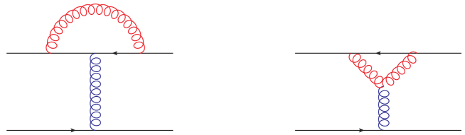
Figure 8: Diagrams whose cuts correspond to virtual processes.

In this appendix we provide a sketch of the diagrammatic evaluation of the diagrams in Fig. 5 in the semi-collinear scaling. In addition, we shall also consider the virtual counterpart, as depicted in Fig. 8. The name labels the fact that the coft gluon is virtual, and transverse momentum exchange happens exclusively via the soft interactions with the medium. The only nonvanishing cut in these diagrams goes through the soft gluon’s HTL, and corresponds to the interference of the leading-order soft scattering with the medium with its coft-gluon-loop virtual correction.

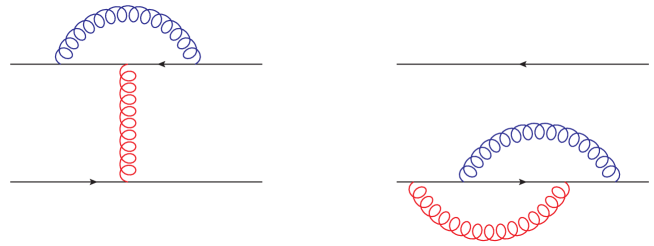
Figure 9: Two type of diagrams that do not contribute to $\mathcal{C}(k_{\perp})$, see main text.

The attentive reader will have noticed that the diagrams of Figs. 5 and 8 do not form the complete set at that order. Missing diagrams are part of two classes. Fig. 9 depicts an example for each. On the left we have diagrams that vanish because their only cut goes through a single coft gluon. Coft gluons have vanishing spectral weight at $k^{-}=0$, which is imposed by the $x^{+}$ integrations at large $L_{\mathrm{med}}$. On the right instead we have $x_{\perp}$-independent diagrams: they thus contribute to the constant part of $\mathcal{C}(x_{\perp})$ which is related to probability conservation. Hence, by looking at Eqs. (21) and (22) we can get the contributions to $\mathcal{C}(k_{\perp})$ by only considering non-vanishing, $x_{\perp}$-dependent diagrams and undoing the overall Fourier transform.

D.1 Real processes

We start from the two diagrams on the top line in Fig. 5. Their combination contains the $C_{R}^{2}$-proportional cross term of the one-coft-gluon exchange with the one-soft-gluon exchange, which is part of the exponentiation of the tree-level contribution. As the one-coft-gluon exchange vanishes for the kinematical reasons just mentioned, only the $C_{R}C_{A}$-proportional, non-abelian piece of the top right diagram survives. It is given by

$$\delta\mathcal{C}(k_{\perp})_{\mathrm{II+X}} =C_{R}C_{A}g^{4}\int\frac{dk^{+}dk^{-}}{(2\pi)^{2}}\int\frac{d^{4}L}{(2\pi)^{4}}\frac{1}{(l^{-}-i\epsilon)^{2}}G_{>}^{--}(K+L)G_{>}^{--}(-L)2\pi\delta(k^{-}).$$ (85)

II and X reflect the topology of the two diagrams, whereas the propagators are both Wightman because of the path-ordering of the fields in the Wilson loop. However, the $L$ propagator is to be understood as soft, and thus HTL-resummed, whereas the $K+L$, being coft, can be taken as bare. A factor of 2 has been added to account for the inverted scaling. Coulomb gauge is implied here and in the rest of the calculation. The $\delta(k^{-})$ arises from the $x^{+}$ integrations at large $L_{\mathrm{med}}$. We do not proceed further with the evaluation, as we prefer to combine all diagrams before.

We now proceed to the self-energy diagram on the bottom left in Fig. 5. Its contribution reads

$$\delta\mathcal{C}(k_{\perp})_{\mathrm{self}}=g^{4}C_{R}C_{A}\int\frac{dk^{+}}{2\pi}\int\frac{d^{4}L}{(2\pi)^{4}}G_{R}^{-\rho}(K)\Big{(}g_{\gamma\sigma}(2L{+}K)_{\rho}-g_{\sigma\rho}(2K{+}L)_{\gamma}+g_{\rho\gamma}(K{-}L)_{\sigma}\Big{)}$$

$$\times G_{>}^{\sigma\delta}(K+L)G_{>}^{\gamma\alpha}(-L)\Big{(}g_{\delta\beta}(2K{+}L)_{\alpha}-g_{\alpha\delta}(2L{+}K)_{\beta}-g_{\alpha\beta}(K{-}L)_{\delta}\Big{)}G_{A}^{\beta-}(K)\Big{|}_{k^{-}=0}.$$ (86)

Cuts going through the $K$ propagators are again vanishing, hence their retarded/advanced assignments only, which is consistent with the cutting rules for Wightman functions Caron-Huot:2007zhp ; Ghiglieri:2020dpq .

Finally, the Y-shaped diagram on the bottom right of Fig. 5, together with its symmetry-related counterparts, yields

$$\delta\mathcal{C}(x_{\perp})_{\mathrm{Y}}= 2g^{4}C_{R}C_{A}\int\frac{dk^{+}d^{2}k_{\perp}}{(2\pi)^{3}}\int\frac{d^{4}L}{(2\pi)^{4}}\frac{i}{l^{-}+i\epsilon}e^{i\bm{k}_{\perp}\cdot\bm{x}_{\perp}}G_{>}^{-\delta}(K+L)G_{>}^{-\alpha}(-L)$$

$$\hskip 34.14322pt\times\Big{(}g_{\alpha\delta}(2L+K)_{\beta}-g_{\delta\beta}(2K+L)_{\alpha}+g_{\beta\alpha}(K-L)_{\delta}\Big{)}G_{F}^{\beta-}(K)\Big{|}_{k^{-}=0}.$$ (87)

At this point, it is useful to write the Feynman propagator as

$$G_{F}(K)=\frac{1}{2}\Big{(}G_{R}(K)+G_{A}(K)\Big{)}+G_{rr}(K).$$ (88)

Since $G_{rr}$ is the average of the bare cut propagators and we have already set $k^{-}=0$, it vanishes. For the same reason, we have not considered the other real-time assignments. That leaves us with the average of the retarded and advanced bare Green’s functions, which when evaluated at $k^{-}=0$ are the same. We can then extract, as was done with the previous diagrams

$$\delta\mathcal{C}(k_{\perp})_{\mathrm{Y}}= -2g^{4}C_{R}C_{A}\int\frac{dk^{+}}{2\pi}\int\frac{d^{4}L}{(2\pi)^{4}}\frac{i}{l^{-}+i\epsilon}G_{>}^{-\delta}(K+L)G_{>}^{-\alpha}(-L)$$

$$\hskip 34.14322pt\times\Big{(}g_{\alpha\delta}(2L+K)_{\beta}-g_{\delta\beta}(2K+L)_{\alpha}+g_{\beta\alpha}(K-L)_{\delta}\Big{)}G_{R}^{\beta-}(K)\Big{|}_{k^{-}=0}.$$ (89)

We can then get the semi-collinear rate by summing the contribution from the three diagrams, i.e.

$$\delta\mathcal{C}(k_{\perp})_{\mathrm{semi}}=\delta\mathcal{C}(k_{\perp})_{\mathrm{II+X}}+\delta\mathcal{C}(k_{\perp})_{\mathrm{self}}+\delta\mathcal{C}(k_{\perp})_{\mathrm{Y}}.$$ (90)

Upon taking care of Lorentz algebra and expanding the resulting expression for the scaling $L\sim gT$, $k^{+}\sim T,k_{\perp}\sim\sqrt{g}T$ we obtain

$$\delta\mathcal{C}(k_{\perp})_{\mathrm{semi}}=4g^{4}C_{R}C_{A}\int\frac{dk^{+}}{2\pi}\int\frac{d^{4}L}{(2\pi)^{4}}\frac{G^{T}_{>}(K+L)}{k_{\perp}^{4}}\Bigg{(} l_{\perp}^{2}G^{--}_{rr}(L)$$

$$+2G^{T}_{rr}(L)\Big{(}{l^{-}}^{2}-\frac{l^{+}l^{-}l_{\perp}^{2}}{l^{2}}\Big{)}\Bigg{)}_{k^{-}=0}.$$ (91)

Upon inserting the form of the bare propagator, expanded under this scaling, we find

$$\delta\mathcal{C}(k_{\perp})_{\mathrm{semi}}= 2g^{4}C_{R}C_{A}\int\frac{dk^{+}}{2\pi}\frac{1+n_{\mathrm{B}}(k^{+})}{k_{\perp}^{4}k^{+}}\int\frac{d^{4}L}{(2\pi)^{3}}\delta\left(l^{-}-\frac{k_{\perp}^{2}}{2k^{+}}\right)\Bigg{(}l_{\perp}^{2}G^{--}_{rr}(L)$$

$$\hskip 142.26378pt+2G^{T}_{rr}(L)\Big{(}{l^{-}}^{2}-\frac{l^{+}l^{-}l_{\perp}^{2}}{l^{2}}\Big{)}\Bigg{)}.$$ (92)

The $l^{+}$ integration can be addressed using light-cone analyticity, as per Ghiglieri:2013gia , leading to Eq. (24).

D.2 Virtual processes

We start from the first diagram in Fig. 8. As was the case for the real II and X diagrams, the $C_{R}^{2}$-proportional, abelian part of this diagram vanishes with the counterparts, not shown in the figure, where the coft gluon does not straddle the soft one. Accounting for this and for the symmetric diagrams with the coft gluon attached to the other Wilson line we have

$$\delta\mathcal{C}(l_{\perp})^{\mathrm{virt}}_{\widehat{\mathrm{T}}}=-g^{4}C_{R}C_{A}\int\frac{d^{4}K}{(2\pi)^{4}}\int\frac{dl^{+}}{2\pi}\frac{1}{(k^{-}+i\epsilon)^{2}}G_{>}^{--}(L)G_{rr}^{--}(K)\Big{|}_{l^{-}=0},$$ (93)

where we have labeled this diagram $\widehat{\mathrm{T}}$ following its topology. We note that the Wilson line integration forces $l^{-}=0$, differently from the real processes. In this case too we defer the evaluation of this expression until after the second diagram has been evaluated. Its contribution, together with that of its symmetric counterpart with two vertices on the bottom Wilson line, is

$$\delta\mathcal{C}(x_{\perp})^{\mathrm{virt}}_{{\mathrm{Y}}}= \frac{g^{4}C_{R}C_{A}}{2}\int\frac{d^{4}K}{(2\pi)^{4}}\int\frac{d^{4}L}{(2\pi)^{4}}\frac{-i}{k^{-}-i\epsilon}e^{i\bm{l}_{\perp}\cdot\bm{x}_{\perp}}G_{>}^{\beta-}(L)2\pi\delta(l^{-})$$

$$\times\big{(}G_{F}^{-\delta}(K)G_{F}^{-\alpha}(K{+}L)-G_{\bar{F}}^{-\delta}(K)G_{\bar{F}}^{-\alpha}(K{+}L)\big{)}(g_{\delta\beta}(K{-}L)+g_{\beta\alpha}(2L{+}K)_{\delta}-g_{\alpha\delta}(2K{+}L)_{\beta}).$$ (94)

We can use the analogue of Eq. (88) for the anti-time-ordered propagator, i.e.

$$G_{\bar{F}}(K)=-\frac{1}{2}\Big{(}G_{R}(K)+G_{A}(K)\Big{)}+G_{rr}(K)$$ (95)

Using these definitions, we get

$$\delta\mathcal{C}(l_{\perp})^{\mathrm{virt}}_{{\mathrm{Y}}}= g^{4}C_{R}C_{A}\int\frac{d^{4}K}{(2\pi)^{4}}\int\frac{dl^{+}dl^{-}}{2\pi}\frac{i}{k^{-}-i\epsilon}G_{>}^{\beta-}(L)\delta(l^{-})$$

$$\times\big{(}G_{rr}^{-\delta}(K)G_{R}^{-\alpha}(K+L)+G_{R}^{-\delta}(K)G_{rr}^{-\alpha}(K+L)\big{)}(g_{\delta\beta}(K{-}L)+g_{\beta\alpha}(2L{+}K)_{\delta}-g_{\alpha\delta}(2K{+}L)_{\beta}).$$ (96)

The virtual contribution is given by the sum of the two, that is

$$\delta\mathcal{C}(l_{\perp})^{\mathrm{virt}}=\delta\mathcal{C}(l_{\perp})^{\mathrm{virt}}_{\widehat{\mathrm{T}}}+\delta\mathcal{C}(l_{\perp})^{\mathrm{virt}}_{{\mathrm{Y}}}.$$ (97)

In this case we do not enforce a semi-collinear scaling for the coft gluon, since, as we shall show, there is no double-logarithmic contribution. Furthermore, the Wilson line integrations set $l^{-}=0$, thus making the interaction with the medium instantaneous. We rather assume $l^{+}\sim l_{\perp}\sim k_{\perp}\sim gT\ll k^{+}$, leading to

$$\delta\mathcal{C}(l_{\perp})^{\mathrm{virt}}= 2g^{4}C_{R}C_{A}\int\frac{dl^{+}}{2\pi}\int\frac{dk^{+}d^{2}k_{\perp}}{(2\pi)^{3}}\frac{\frac{1}{2}+n_{\mathrm{B}}(k^{+})}{k^{+}}\frac{G^{--}_{>}(l^{+},l_{\perp})}{k_{\perp}^{2}+m_{\infty\,g}^{2}}$$

$$\times\bigg{[}\frac{k_{\perp}^{2}+\bm{k}_{\perp}\cdot\bm{l}_{\perp}}{(\bm{k}_{\perp}+\bm{l}_{\perp})^{2}+m_{\infty\,g}^{2}}-\frac{k_{\perp}^{2}}{k_{\perp}^{2}+m_{\infty g}^{2}}\bigg{]}.$$ (98)

The asymptotic masses at the denominator have been included since we assumed $k_{\perp}\sim gT$. They arise from the $k^{+}\sim T$, $K^{2}\sim g^{2}T^{2}$ limit of the HTL propagators in App. A. The $l^{+}$ integration can be carried out through the mapping to EQCD, as summarized around Eq. (31). It leads to

$$\delta\mathcal{C}(l_{\perp})^{\mathrm{virt}}= 2g^{4}C_{R}C_{A}\int\frac{dk^{+}d^{2}k_{\perp}}{(2\pi)^{3}}\frac{\frac{1}{2}+n_{\mathrm{B}}(k^{+})}{k^{+}}\frac{Tm_{D}^{2}}{l_{\perp}^{2}(l_{\perp}^{2}+m_{D}^{2})}\frac{1}{k_{\perp}^{2}+m_{\infty\,g}^{2}}$$

$$\times\bigg{[}\frac{k_{\perp}^{2}+\bm{k}_{\perp}\cdot\bm{l}_{\perp}}{(\bm{k}_{\perp}+\bm{l}_{\perp})^{2}+m_{\infty\,g}^{2}}-\frac{k_{\perp}^{2}}{k_{\perp}^{2}+m_{\infty\,g}^{2}}\bigg{]}.$$ (99)

We recognize that this expression is proportional to the leading-order, adjoint soft scattering kernel $\mathcal{C}(l_{\perp})^{\mathrm{LO}}_{\mathrm{soft}}$, Eq. (51). From this expression and its associated $\hat{q}$ contribution one can see that the $|\bm{k}_{\perp}+\bm{l}_{\perp}|\gg l_{\perp}$ single-scattering region is free of double-logarithmic enhancements, as found in Liou:2013qya . Furthermore, for $k_{\perp}\sim l_{\perp}\sim gT$, which we have used for our derivation, the lifetime of the virtual coft fluctuation is long, so that multiple soft scatterings can occur within it. Hence, Eq. (99) should just be considered as the $N=1$ term in the opacity expansion of the virtual contribution to Eq. (43). Indeed, we have checked that Eq. (99) can also be obtained from the virtual terms in Eq. (45), i.e. those proportional to $\exp(i\bm{x}_{\perp}\cdot\bm{l}_{\perp})$, further confirming the soundness of Eqs. (41) and (43).

References

• (1) M. Connors, C. Nattrass, R. Reed and S. Salur, Jet measurements in heavy ion physics, Rev. Mod. Phys. 90 (2018) 025005 [1705.01974].
• (2) S. Cao and X.-N. Wang, Jet quenching and medium response in high-energy heavy-ion collisions: a review, Rept. Prog. Phys. 84 (2021) 024301 [2002.04028].
• (3) L. Cunqueiro and A.M. Sickles, Studying the QGP with Jets at the LHC and RHIC, Prog. Part. Nucl. Phys. 124 (2022) 103940 [2110.14490].
• (4) L. Apolinário, Y.-J. Lee and M. Winn, Heavy quarks and jets as probes of the QGP, 2203.16352.
• (5) JET collaboration, Extracting the jet transport coefficient from jet quenching in high-energy heavy-ion collisions, Phys.Rev. C90 (2014) 014909 [1312.5003].
• (6) C. Andrés, N. Armesto, M. Luzum, C.A. Salgado and P. Zurita, Energy versus centrality dependence of the jet quenching parameter $\hat{q}$ at RHIC and LHC: a new puzzle?, The European Physical Journal C 76 (2016) [hep-ph/1606.04837].
• (7) M. Xie, S.-Y. Wei, G.-Y. Qin and H.-Z. Zhang, Extracting jet transport coefficient via single hadron and dihadron productions in high-energy heavy-ion collisions, Eur. Phys. J. C 79 (2019) 589 [1901.04155].
• (8) A. Huss, A. Kurkela, A. Mazeliauskas, R. Paatelainen, W. van der Schee and U.A. Wiedemann, Predicting parton energy loss in small collision systems, Phys. Rev. C 103 (2021) 054903 [2007.13758].
• (9) JETSCAPE collaboration, Determining the jet transport coefficient $\hat{q}$ from inclusive hadron suppression measurements using Bayesian parameter estimation, Phys. Rev. C 104 (2021) 024905 [2102.11337].
• (10) Q.-F. Han, M. Xie and H.-Z. Zhang, Extracting the jet transport coefficient from hadron suppressions by confronting current NLO parton fragmentation functions, 2201.02796.
• (11) M. Xie, W. Ke, H. Zhang and X.-N. Wang, Information field based global Bayesian inference of the jet transport coefficient, 2206.01340.
• (12) E. Braaten and R.D. Pisarski, Soft Amplitudes in Hot Gauge Theories: A General Analysis, Nucl.Phys. B337 (1990) 569.
• (13) P. Aurenche, F. Gelis and H. Zaraket, A Simple sum rule for the thermal gluon spectral function and applications, JHEP 0205 (2002) 043 [hep-ph/0204146].
• (14) P.B. Arnold and W. Xiao, High-energy jet quenching in weakly-coupled quark-gluon plasmas, Phys.Rev. D78 (2008) 125008 [0810.1026].
• (15) A.D. Linde, Infrared Problem in Thermodynamics of the Yang-Mills Gas, Phys.Lett. B96 (1980) 289.
• (16) M. Laine, A non-perturbative contribution to jet quenching, Eur.Phys.J. C72 (2012) 2233 [1208.5707].
• (17) S. Caron-Huot, O(g) plasma effects in jet quenching, Phys.Rev. D79 (2009) 065039 [0811.1603].
• (18) E. Braaten, Solution to the perturbative infrared catastrophe of hot gauge theories, Phys.Rev.Lett. 74 (1995) 2164 [hep-ph/9409434].
• (19) E. Braaten and A. Nieto, Effective field theory approach to high temperature thermodynamics, Phys.Rev. D51 (1995) 6990 [hep-ph/9501375].
• (20) E. Braaten and A. Nieto, Free energy of QCD at high temperature, Phys.Rev. D53 (1996) 3421 [hep-ph/9510408].
• (21) K. Kajantie, M. Laine, K. Rummukainen and M.E. Shaposhnikov, Generic rules for high temperature dimensional reduction and their application to the standard model, Nucl.Phys. B458 (1996) 90 [hep-ph/9508379].
• (22) K. Kajantie, M. Laine, K. Rummukainen and M.E. Shaposhnikov, 3-D SU(N) + adjoint Higgs theory and finite temperature QCD, Nucl.Phys. B503 (1997) 357 [hep-ph/9704416].
• (23) M. Panero, K. Rummukainen and A. Schäfer, A lattice study of the jet quenching parameter, Phys.Rev.Lett. 112 (2014) 162001 [1307.5850].
• (24) G.D. Moore and N. Schlusser, Transverse momentum broadening from the lattice, Phys. Rev. D 101 (2020) 014505 [1911.13127].
• (25) M. Laine and A. Rothkopf, Light-cone Wilson loop in classical lattice gauge theory, JHEP 1307 (2013) 082 [1304.4443].
• (26) G.D. Moore, S. Schlichting, N. Schlusser and I. Soudi, Non-perturbative determination of collisional broadening and medium induced radiation in QCD plasmas, JHEP 10 (2021) 059 [2105.01679].
• (27) S. Schlichting and I. Soudi, Splitting rates in QCD plasmas from a nonperturbative determination of the momentum broadening kernel $C(q_{\perp})$, Phys. Rev. D 105 (2022) 076002 [2111.13731].
• (28) B. Wu, On $p_{\bot}$-broadening of high energy partons associated with the LPM effect in a finite-volume QCD medium, JHEP 10 (2011) 029 [1102.0388].
• (29) T. Liou, A. Mueller and B. Wu, Radiative $p_{\bot}$-broadening of high-energy quarks and gluons in QCD matter, Nucl.Phys. A916 (2013) 102 [1304.7677].
• (30) J.-P. Blaizot, F. Dominguez, E. Iancu and Y. Mehtar-Tani, Probabilistic picture for medium-induced jet evolution, JHEP 1406 (2014) 075 [1311.5823].
• (31) J.-P. Blaizot and Y. Mehtar-Tani, Jet Structure in Heavy Ion Collisions, Int. J. Mod. Phys. E24 (2015) 1530012 [1503.05958].
• (32) E. Iancu, The non-linear evolution of jet quenching, JHEP 10 (2014) 095 [1403.1996].
• (33) E. Iancu and D.N. Triantafyllopoulos, Running coupling effects in the evolution of jet quenching, Phys. Rev. D 90 (2014) 074002 [1405.3525].
• (34) P. Caucal and Y. Mehtar-Tani, Anomalous diffusion in QCD matter, 2109.12041.
• (35) P. Caucal and Y. Mehtar-Tani, Universality aspects of quantum corrections to transverse momentum broadening in QCD media, 2203.09407.
• (36) J.-P. Blaizot and F. Dominguez, Radiative corrections to the jet quenching parameter in dilute and dense media, Phys. Rev. D 99 (2019) 054005 [1901.01448].
• (37) J.-P. Blaizot and Y. Mehtar-Tani, Renormalization of the jet-quenching parameter, Nucl. Phys. A 929 (2014) 202 [1403.2323].
• (38) B. Wu, Radiative energy loss and radiative $p_{\bot}$-broadening of high-energy partons in QCD matter, JHEP 12 (2014) 081 [1408.5459].
• (39) P. Arnold and S. Iqbal, The LPM effect in sequential bremsstrahlung, JHEP 1504 (2015) 070 [1501.04964].
• (40) P. Arnold, H.-C. Chang and S. Iqbal, The LPM effect in sequential bremsstrahlung 2: factorization, JHEP 09 (2016) 078 [1605.07624].
• (41) P. Arnold, H.-C. Chang and S. Iqbal, The LPM effect in sequential bremsstrahlung: dimensional regularization, JHEP 10 (2016) 100 [1606.08853].
• (42) P. Arnold and S. Iqbal, In-medium loop corrections and longitudinally polarized gauge bosons in high-energy showers, JHEP 12 (2018) 120 [1806.08796].
• (43) P. Arnold, S. Iqbal and T. Rase, Strong- vs. weak-coupling pictures of jet quenching: a dry run using QED, JHEP 05 (2019) 004 [1810.06578].
• (44) P. Arnold, Landau-Pomeranchuk-Migdal effect in sequential bremsstrahlung: From large-$N$ QCD to $N$=3 via the SU($N$) analog of Wigner 6-$j$ symbols, Phys. Rev. D 100 (2019) 034030 [1904.04264].
• (45) P. Arnold, T. Gorda and S. Iqbal, The LPM effect in sequential bremsstrahlung: nearly complete results for QCD, JHEP 11 (2020) 053 [2007.15018].
• (46) P. Arnold, T. Gorda and S. Iqbal, The LPM effect in sequential bremsstrahlung: analytic results for sub-leading (single) logarithms, JHEP 04 (2022) 085 [2112.05161].
• (47) P. Arnold and O. Elgedawy, The LPM Effect in sequential bremsstrahlung: $1/N_{c}^{2}$ corrections, 2202.04662.
• (48) P. Arnold, Universality (beyond leading log) of soft radiative corrections to $\hat{q}$ in $p_{\perp}$ broadening and energy loss, JHEP 03 (2022) 134 [2111.05348].
• (49) G. Moliere, Theorie der Streuung schneller geladener Teilchen I. Einzelstreuung am abgeschirmten Coulomb-Feld, Z. Naturforsch. A2 (1947) 133.
• (50) G. Moliere, Theory of the scattering of fast charged particles. 2. Repeated and multiple scattering, Z. Naturforsch. A3 (1948) 78.
• (51) F. D’Eramo, K. Rajagopal and Y. Yin, Molière scattering in quark-gluon plasma: finding point-like scatterers in a liquid, JHEP 01 (2019) 172 [1808.03250].
• (52) T. Dai, J.-F. Paquet, D. Teaney and S.A. Bass, Parton energy loss in a hard-soft factorized approach, Phys. Rev. C 105 (2022) 034905 [2012.03441].
• (53) P.B. Arnold, G.D. Moore and L.G. Yaffe, Effective kinetic theory for high temperature gauge theories, JHEP 0301 (2003) 030 [hep-ph/0209353].
• (54) J. Ghiglieri, G.D. Moore and D. Teaney, Jet-Medium Interactions at NLO in a Weakly-Coupled Quark-Gluon Plasma, JHEP 03 (2016) 095 [1509.07773].
• (55) P.B. Arnold and C. Dogan, QCD Splitting/Joining Functions at Finite Temperature in the Deep LPM Regime, Phys. Rev. D 78 (2008) 065008 [0804.3359].
• (56) P.B. Arnold, Quark-Gluon Plasmas and Thermalization, Int. J. Mod. Phys. E 16 (2007) 2555 [0708.0812].
• (57) P.B. Arnold, G.D. Moore and L.G. Yaffe, Photon emission from ultrarelativistic plasmas, JHEP 0111 (2001) 057 [hep-ph/0109064].
• (58) P.B. Arnold, G.D. Moore and L.G. Yaffe, Photon and gluon emission in relativistic plasmas, JHEP 0206 (2002) 030 [hep-ph/0204343].
• (59) J. Ghiglieri, J. Hong, A. Kurkela, E. Lu, G.D. Moore and D. Teaney, Next-to-leading order thermal photon production in a weakly coupled quark-gluon plasma, JHEP 1305 (2013) 010 [1302.5970].
• (60) R. Baier, Y.L. Dokshitzer, A.H. Mueller, S. Peigne and D. Schiff, Radiative energy loss of high-energy quarks and gluons in a finite volume quark - gluon plasma, Nucl.Phys. B483 (1997) 291 [hep-ph/9607355].
• (61) U.W. Heinz, K. Kajantie and T. Toimela, Gauge Covariant Linear Response Analysis of QCD Plasma Oscillations, Annals Phys. 176 (1987) 218.
• (62) N. Brambilla, M.A. Escobedo, J. Ghiglieri, J. Soto and A. Vairo, Heavy Quarkonium in a weakly-coupled quark-gluon plasma below the melting temperature, JHEP 09 (2010) 038 [1007.4156].
• (63) M.A. Escobedo and J. Soto, Non-relativistic bound states at finite temperature (II): the muonic hydrogen, Phys. Rev. A 82 (2010) 042506 [1008.0254].
• (64) C. Manuel, J. Soto and S. Stetina, On-shell effective field theory: A systematic tool to compute power corrections to the hard thermal loops, Phys. Rev. D 94 (2016) 025017 [1603.05514].
• (65) S. Carignano, C. Manuel and J. Soto, Power corrections to the HTL effective Lagrangian of QED, Phys. Lett. B 780 (2018) 308 [1712.07949].
• (66) J. Casalderrey-Solana and D. Teaney, Transverse Momentum Broadening of a Fast Quark in a N=4 Yang Mills Plasma, JHEP 04 (2007) 039 [hep-th/0701123].
• (67) F. D’Eramo, H. Liu and K. Rajagopal, Transverse Momentum Broadening and the Jet Quenching Parameter, Redux, Phys.Rev. D84 (2011) 065015 [1006.1367].
• (68) M. Benzke, N. Brambilla, M.A. Escobedo and A. Vairo, Gauge invariant definition of the jet quenching parameter, JHEP 1302 (2013) 129 [1208.4253].
• (69) T. Becher, M. Neubert, L. Rothen and D.Y. Shao, Effective Field Theory for Jet Processes, Phys. Rev. Lett. 116 (2016) 192001 [1508.06645].
• (70) J. Ghiglieri and D. Teaney, Parton energy loss and momentum broadening at NLO in high temperature QCD plasmas, Int. J. Mod. Phys. E24 (2015) 1530013 [1502.03730].
• (71) P.B. Arnold, G.D. Moore and L.G. Yaffe, Transport coefficients in high temperature gauge theories. 2. Beyond leading log, JHEP 0305 (2003) 051 [hep-ph/0302165].
• (72) S. Caron-Huot, On supersymmetry at finite temperature, Phys.Rev. D79 (2009) 125002 [0808.0155].
• (73) G.D. Moore and N. Schlusser, The nonperturbative contribution to asymptotic masses, Phys. Rev. D 102 (2020) 094512 [2009.06614].
• (74) J. Ghiglieri, G.D. Moore, P. Schicho and N. Schlusser, The force-force-correlator in hot QCD perturbatively and from the lattice, JHEP 02 (2022) 058 [2112.01407].
• (75) J. Ghiglieri and H. Kim, Transverse momentum broadening and collinear radiation at NLO in the $\mathcal{N}=4$ SYM plasma, JHEP 12 (2018) 049 [1809.01349].
• (76) S. Caron-Huot and C. Gale, Finite-size effects on the radiative energy loss of a fast parton in hot and dense strongly interacting matter, Phys.Rev. C82 (2010) 064902 [1006.2379].
• (77) C. Andres, L. Apolinário and F. Dominguez, Medium-induced gluon radiation with full resummation of multiple scatterings for realistic parton-medium interactions, JHEP 07 (2020) 114 [2002.01517].
• (78) C. Andres, F. Dominguez and M. Gonzalez Martinez, From soft to hard radiation: the role of multiple scatterings in medium-induced gluon emissions, JHEP 03 (2021) 102 [2011.06522].
• (79) Y. Mehtar-Tani and K. Tywoniuk, Improved opacity expansion for medium-induced parton splitting, JHEP 06 (2020) 187 [1910.02032].
• (80) J.a. Barata, Y. Mehtar-Tani, A. Soto-Ontoso and K. Tywoniuk, Revisiting transverse momentum broadening in dense QCD media, Phys. Rev. D 104 (2021) 054047 [2009.13667].
• (81) J.a. Barata, Y. Mehtar-Tani, A. Soto-Ontoso and K. Tywoniuk, Medium-induced radiative kernel with the Improved Opacity Expansion, JHEP 09 (2021) 153 [2106.07402].
• (82) J.H. Isaksen, A. Takacs and K. Tywoniuk, A unified picture of medium-induced radiation, 2206.02811.
• (83) J. Ghiglieri, A. Kurkela, M. Strickland and A. Vuorinen, Perturbative Thermal QCD: Formalism and Applications, Phys. Rept. 880 (2020) 1 [2002.10188].
• (84) S. Caron-Huot, Heavy quark energy losses in the quark-gluon plasma : beyond leading order, Master’s thesis, McGill U., 2007.