Iterative solution of spatial network models by subspace decomposition

Abstract

We present and analyze a preconditioned conjugate gradient method (PCG) for solving spatial network problems. Primarily, we consider diffusion and structural mechanics simulations for fiber based materials, but the methodology can be applied to a wide range of models, fulfilling a set of abstract assumptions. The proposed method builds on a classical subspace decomposition into a coarse subspace, realized as the restriction of a finite element space to the nodes of the spatial network, and localized subspaces with support on mesh stars. The main contribution of this work is the convergence analysis of the proposed method. The analysis translates results from finite element theory, including interpolation bounds, to the spatial network setting. A convergence rate of the PCG algorithm, only depending on global bounds of the operator and homogeneity, connectivity and locality constants of the network, is established. The theoretical results are confirmed by several numerical experiments.

1 Introduction

Many phenomena in science and engineering, modelled by partial differential equations (PDE), are challenging to simulate accurately due to their vast complexity. Sometimes it is beneficial to simplify, still maintaining the main features of the full model, by introducing a spatial network model. In porous media flow modelling, see Figure 1.1 (left), the flow in the exact pore geometry can be approximated by a simplified network model of edges (throats) and nodes (pore cavities), see [1, 12, 14]. This technique reduces the computational complexity and allows for simulation using larger computational domains. A fiber based material such as paper, see Figure 1.1 (right), can also be modelled using a spatial network model where the three dimensional hollow cylindrical fibers are modelled as one dimensional objects, represented by edges connected with nodes, and the contact regions as additional nodes, see [13, 15, 16]. Even though much of the complexity is eliminated in this way, it is still often challenging to solve the resulting model efficiently.

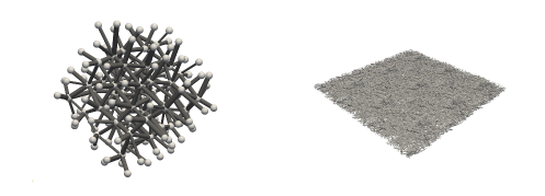
Figure 1.1: Illustration of a subgraph in a pore network model (left) and a fiber network model (millimeter scale) of paper (right).

In this paper, we consider spatial network models that arise from applications modelled by linear elliptic partial differential equations such as heat conduction and structural mechanics. The corresponding system matrices are weighted graph Laplacians in the scalar case and related to the weighted graph Laplacians in each coordinate direction in the vector valued case. Successful numerical algorithms for solving the resulting sparse linear systems use parallelization and discretizations on a range of scales. This is exploited in iterative methods such as geometric and algebraic multigrid [2, 24, 26] and domain decomposition [21, 23]. In a PDE setting with a simple geometry it is natural to introduce nested discretizations on different levels. In a purely algebraic setting it is less obvious but there are many coarsening techniques available that uses connectivity information from the system matrix, see for instance [24, 26]. There are geometry based algebraic multigrid methods that uses some geometrical information to construct levels of coarsening [26]. This setting is most similar to the model we study.

We consider a spatial network defined by a graph $\mathcal{G}=\{\mathcal{N},\mathcal{E}\}$ of nodes and edges. The nodes and edges are contained in a bounded domain $\Omega$. The model problem is defined by a symmetric linear operator $\mathbf{K}$ and a right hand side $\mathbf{f}$. The operator act on a linear space $\mathbf{V}$ of functions defined on $\mathcal{N}$. We want to solve a stationary equation of the form: find $\mathbf{u}\in\mathbf{V}$ such that for all $\mathbf{v}\in\mathbf{V}$,

$$(\mathbf{K}\mathbf{u},\mathbf{v})=(\mathbf{f},\mathbf{v}).$$

We introduce a coarse finite element discretization of $\Omega$ and let $\mathbf{V}_{H}\subset\mathbf{V}$ be its restriction to the network. The full solution space $\mathbf{V}$ is then decomposed into $\mathbf{V}_{0}=\mathbf{V}_{H}$ and a set of overlapping local subspaces $\{\mathbf{V}_{j}\}_{j=1}^{m}$. Given the subspace decomposition we formulate an additive Schwarz preconditioner for the model problem and apply the conjugate gradient method to the preconditioned system. The main theoretical contribution of this work is the convergence proof of the proposed scheme, with a rate that only depends on global bounds on $\mathbf{K}$ and the homogeneity, connectivity and locality of the network on a scale $R_{0}$, under the additional assumption that $H\geq R_{0}$. These dependencies are traced explicitly in the analysis and reveals the impact of the $R_{0}$-scale homogeneity and connectivity on the convergence of the iterative solver. To prove the main result we translate results from finite element theory to the network setting including the construction of an interpolation operator, the proof of interpolation bounds, and the proof of a product rule type bound. The interpolation bound in turn builds on Poincaré and Friedrichs inequalities on subgraphs, see [4, 5] and the earlier contributions [3, 9]. By this we establish spectral bounds of the preconditioned operator. Given the spectral bounds we apply classical additive Schwarz theory to prove the convergence, see [18, 25]. In the first numerical experiment we consider a randomly generated model of a fiber based material, defined by fiber length and density. We investigate how the homogeneity and connectivity constants depends on the parameters in the model and the size of the domain. Then we present a scalar (heat conductivity) and a vector (structural mechanical model) valued numerical example which shows the efficiency of the proposed method for models of fiber based materials.

The paper is organized as follows. Section 2 is devoted to preliminary notation and Section 3 to problem formulation and assumptions on the operator $\mathbf{K}$ and the network. In Section 4 we introduce a preconditioned conjugate gradient method and present the main convergence result. Section 5 is devoted to the proof of the spectral bound of the preconditioned operator which is the main technical result needed for the convergence proof. Finally, in Section 6 we present numerical examples.

2 Preliminary notation

We start by introducing notation for the spatial network itself and for operators defined on the network. We also introduce finite element spaces that are restricted to the network and used in the subspace decomposition.

2.1 Spatial network

We consider a connected spatial network represented as the graph $\mathcal{G}=(\mathcal{N},\mathcal{E})$. The node set $\mathcal{N}$ is a finite set of points in $\mathbb{R}^{d}$ and the edge set

$$\mathcal{E}=\{\{x,y\}\,:\,\text{an edge connects }x\text{ and }y\in\mathcal{N}\}$$

consists of unordered pairs of the endpoint vertices of each edge. The notation $x\sim y$ expresses that $\{x,y\}$ is an edge in $\mathcal{E}$. If $x\sim y$, then we say that the nodes $x$ and $y$ are adjacent. If two nodes $x$ and $y$ are adjacent then $|x-y|$ is the length of the edge connecting them, with $|\cdot|$ being the Euclidean norm. The network is embedded in a spatial domain $\Omega$ ($\mathcal{N}\subset\Omega$), which we for simplicity assume to be the closed hyper-rectangle

$$\Omega=[0,l_{1}]\times[0,l_{2}]\times\dots\times[0,l_{d}]\subset\mathbb{R}^{d}.$$

In Remarks 2.1 we discuss how the methodology can be modified for general polygonal/polyhedral domains. We let $\Gamma\subset\partial\Omega$ be the part of the boundary of $\Omega$ on which homogeneous Dirichlet boundary conditions are applied, see Figure 2.1.

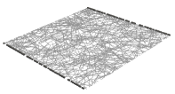
Figure 2.1: Dirichlet nodes on a subset $\Gamma$ of the boundary of the domain $\Omega$.

We let $\hat{V}$ be the space of real-valued functions defined on the node set $\mathcal{N}$ and let

$$V=\{v\in\hat{V}\,:\,v(x)=0,x\in\Gamma\}$$

denote the function set satisfying the boundary conditions. For two functions $u,v\in\hat{V}$, we define the node-wise product $uv\in\hat{V}$ in the natural way i.e. $(uv)(x)=u(x)v(x)$ for $x\in\mathcal{N}$. When $\omega\subset\Omega$, we define $\mathcal{N}(\omega)=\mathcal{N}\cap\omega$.

2.2 Operators and norms

For $u,v\in\hat{V}$ we define the inner product

$$(u,v)=(u,v)_{\Omega}\quad\text{where}\quad(u,v)_{\omega}=\sum_{x\in\mathcal{N}(\omega)}u(x)v(x).$$

For every node in the network, $x\in\mathcal{N}$, let $M_{x}:\hat{V}\to\hat{V}$ be the diagonal linear operator defined by

$$(M_{x}v,v)=\frac{1}{2}\sum_{x\sim y}|x-y|v(x)^{2}.$$ (2.1)

By $\sum_{x\sim y}$ we mean that the sum goes over all nodes $y$ adjacent to the given $x$. For subdomains $\omega\subset\Omega$ we introduce the shorthand notation $M_{\omega}=\sum_{x\in\mathcal{N}(\omega)}M_{x}$, and $M=M_{\Omega}$. Note that $M:\hat{V}\rightarrow\hat{V}$ but, if we restrict the domain, also $M:V\rightarrow V$ holds. We define the norm $|v|_{M}=(Mv,v)^{1/2}$ and the semi-norms $|v|_{M,\omega}=(M_{\omega}v,v)^{1/2}$.

Next we define the reciprocal edge length weighted graph Laplacian. Let $L_{x}:\hat{V}\to\hat{V}$ be defined by

$$(L_{x}v,v)=\frac{1}{2}\sum_{x\sim y}\frac{(v(x)-v(y))^{2}}{|x-y|}.$$ (2.2)

Again we introduce the shorthand notation for subdomains $\omega\subset\Omega$, $L_{\omega}=\sum_{x\in\mathcal{N}(\omega)}L_{x}$, and $L=L_{\Omega}$. Note that $(L_{\omega}u)(x)$ is generally nonzero for vertices $x$ outside $\omega$ that are adjacent to a node in $\omega$. The weighted Laplacian $L$ is symmetric and positive semi-definite and the kernel of $L$ contains the constant functions in $\hat{V}$. Since we assume that the network is connected, the kernel of $L$ has dimension one. The operator $L$ defines the following semi-norms, $|v|_{L}=(Lv,v)^{1/2}$ and $|v|_{L,\omega}=(L_{\omega}v,v)^{1/2}$. The notation $V(\omega)$ will be used to denote the space of functions that are zero for nodes outside $\omega$.

To handle both scalar and vector valued functions we introduce vector-valued functions of $n$ components, where for example $n=1$ or $n=d$. We introduce the product space

$$\mathbf{V}=V^{n}=V\times\cdots\times V\qquad\text{(}n\text{ times)}$$

as the admissible function space for the unknown and the full space $\mathbf{\hat{V}}={\hat{V}}^{n}$ (so that $\mathbf{V}\subset\mathbf{\hat{V}}$). The components of $\mathbf{V}$ need not be identical if different boundary conditions are applied to the components, however, for simplicity we assume that all components are identical. A function $\mathbf{v}\in\mathbf{\hat{V}}$ consists of the components $\mathbf{v}=[v_{1},v_{2},\ldots,v_{n}]$ subscripted by their index. We introduce $\mathbf{L}_{x}:\hat{\mathbf{V}}\to\hat{\mathbf{V}}$ as $L_{x}$ applied componentwise, i.e.

$$\mathbf{L}_{x}\mathbf{v}=[L_{x}v_{1},\ldots,L_{x}v_{n}].$$

For $\omega\in\Omega$, we let $\mathbf{L}_{\omega}=\sum_{x\in\mathcal{N}(\omega)}\mathbf{L}_{x}$ and $\mathbf{L}=\mathbf{L}_{\Omega}$. We also extend the notation for the inner product to the product space by

$$(\mathbf{u},\mathbf{v})=(u_{1},v_{1})+\cdots+(u_{n},v_{n})$$

and introduce the semi-norms

$$|\mathbf{v}|_{\mathbf{L},\omega}=(\mathbf{L}_{\omega}\mathbf{v},\mathbf{v})^{1/2}=\left(|v_{1}|_{L,\omega}^{2}+\cdots+|v_{n}|_{L,\omega}^{2}\right)^{1/2}$$

and shorthand $|\mathbf{v}|_{\mathbf{L}}=|\mathbf{v}|_{\mathbf{L},\Omega}$. The analogue notation for $\mathbf{M}$ will also be used.

2.3 Finite element mesh and function space

The preconditioner we propose for the iterative solver uses a coarser scale representations of the full network. To construct this representation we first introduce a family of finite element meshes on the spatial domain $\Omega$. The construction we consider has been used previously to handle non-nested meshes in the localized orthogonal decomposition method, see [20, 19]. To be able to emphasize the main message of the paper, we choose a simple mesh of hypercubes (squares for $d=2$, and cubes for $d=3$, etc.).

We introduce boxes $B_{R}(x)\subset\Omega$ centered at $x=(x_{1},\ldots,x_{d})$ with side length $2R$ as follows. Let

$$B_{R}(x)=[x_{1}-R,x_{1}+R)\times\cdots\times[x_{d}-R,x_{d}+R),$$

but replace $[x_{i}-R,x_{i}+R)$ with $[x_{i}-R,x_{i}+R]$ for any $i$ for which $x_{i}+R=l_{i}$. In this way, $B_{R}(x)$ only include its upper boundary of any dimension if it intersects the boundary of $\Omega$. We let $\mathcal{T}_{H}$ be a family of partitions (meshes) of $\Omega$ into hypercubes (elements) of side length $H$:

$$\mathcal{T}_{H}=\{B_{H/2}(x)\,:\,x=(x_{1},\ldots,x_{d})\in\Omega\text{ and }H^{-1}x_{i}+1/2\in\mathbb{Z}\text{ for }i=1,\ldots,d\}.$$

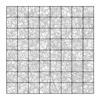
Figure 2.2: The finite element mesh $\mathcal{T}_{H}$ with a network in the background.

For simplicity, we assume the side lengths of the hyper-rectangle $l_{1},l_{2},\dots,l_{d}$ are integer multiples of a mesh parameter $H$ so that $\mathcal{T}_{H}$ exactly covers $\Omega$. By the construction of $B_{R}(x)$, $\mathcal{T}_{H}$ is a true partition so that each point in $\Omega$ is included in exactly one element, see Figure 2.2.

To name patches of elements in a mesh $\mathcal{T}_{H}$, we introduce the notation $U$. For $\omega\subset\Omega$ let

$$U(\omega)=\{x\in\Omega\,:\,\exists T\in\mathcal{T}_{H}\,:\,x\in T,\ \overline{T}\cap\overline{\omega}\neq\emptyset\}.$$

The patch $U(T)$ contains the points in $T$ and its adjacent elements. Recursively, we define larger patches $U_{j}(\omega)=U_{j-1}(U(\omega))$ with $U_{1}=U$. By this construction, $U_{2}(T)=U(U(T))$ contains the points in all elements in the element patch for $T$ with “radius” 2. Moreover, the definition of $U$ is extended to accept arguments that are individual points, by $U(x)=U(\{x\})$ when $x\in\Omega$, see Figure 2.3.

We now introduce a first-order finite element space on the mesh $\mathcal{T}_{H}$. Let $\mathcal{\hat{Q}}_{H}$ be the space of continuous functions defined on $\Omega$ whose restriction to $T\in\mathcal{T}_{H}$ is a linear combination of the polynomials $z=(z_{1},\ldots,z_{d})\mapsto z^{\alpha}$ for multi-index $\alpha$ with $|\alpha|\leq 1$. For $d=2$, this is the space of bilinear functions on $T$. Further, let $\mathcal{Q}_{H}=\{q\in\mathcal{\hat{Q}}_{H}\,:\,q(x)=0,x\in\Gamma\}$.

We are interested in the restriction of these functions to the network nodes. Let $\hat{V}_{H}$ be the functions in $\mathcal{\hat{Q}}_{H}$ restricted to $\mathcal{N}$, with $V_{H}$ similarly defined. We further define the function space $\mathbf{V}_{H}$ of vector-valued functions by

$$\mathbf{V}_{H}=V_{H}\times\cdots\times V_{H}\qquad\text{(}n\text{ times)}.$$

From now on we consider a fix $H$ and omit subscript $H$ in new notation. Let $m$ be the dimension of $\mathcal{\hat{Q}}_{H}$, and denote the Lagrange finite element basis functions by $\varphi_{1},\ldots,\varphi_{m}\in\mathcal{\hat{Q}}_{H}$, and their restrictions to the network nodes again denoted by $\varphi_{1},\ldots,\varphi_{m}\in\hat{V}_{H}$, see Figure 2.3. The nodes of the mesh $\mathcal{T}_{H}$ are denoted $y_{1},\ldots,y_{m}$. Note that we do not require that the mesh nodes coincide with network nodes in $\mathcal{N}$.

We assume that the mesh is aligned with $\Gamma$ in the sense that $\Gamma$ can be expressed as a union of element faces. Without loss of generality we order the basis function such that the $m_{0}<m$ first basis functions $\varphi_{1},\ldots,\varphi_{m_{0}}$ span $\mathcal{Q}_{H}$.

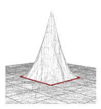
Figure 2.3: The basis function $\varphi_{j}$ with corresponding patch $U(y_{j})$ in red.

Remark 2.1.

If the domain $\Omega$ is a general polygonal/polyhedral domain we instead use a finite element space based on continuous piecewise affine functions on a shape regular mesh of $d$-simplices (triangles for $d=2$ and tetrahedra for $d=3$). Every node in the network is assigned to exactly one element. If a point belongs to the closure of several elements we assign it to the one with the lowest element number. Once the elements are constructed and the nodes are distributed to the elements, element patches $U$ can again be defined as above.

3 Problem formulation and assumptions

In this section we introduce the model problem. We also state assumptions on the linear operator $\mathbf{K}$, defining the interactions over the network, and the network itself needed to prove our main convergence result.

The model problem is expressed in terms of a symmetric and positive semi-definite linear operator $\mathbf{K}:\hat{\mathbf{V}}\to\hat{\mathbf{V}}$ and a right hand side function $\mathbf{f}\in\hat{\mathbf{V}}$: find $\mathbf{u}\in\mathbf{V}$ such that for all $\mathbf{v}\in\mathbf{V}$,

$$(\mathbf{K}\mathbf{u},\mathbf{v})=(\mathbf{f},\mathbf{v}).$$ (3.1)

Since $\mathbf{u}\in\mathbf{V}$, the solution is zero in the non-empty set of nodes $\mathcal{N}(\Gamma)$ where $\Gamma\subset\partial\Omega$ is the Dirichlet boundary. If the sought solution is equal to some given non-zero function $\mathbf{g}(x)$ for $x\in\mathcal{N}(\Gamma)$, we extend $\mathbf{g}$ to all nodes, let the sought solution be $\hat{\mathbf{u}}=\mathbf{u}+\mathbf{g}$, and solve for $\mathbf{u}\in\mathbf{V}$ with modified right hand side instead. Non-zero flux boundary conditions can be added in the right hand side of equation (3.1).

3.1 Assumptions on $\mathbf{K}$

We restrict our attention to operators with the following properties:

Assumption 3.1.

The operator $\mathbf{K}$

1. is bounded and coercive on $\mathbf{V}$ with respect to $\mathbf{L}$, i.e. there are constants $\alpha>0$ and $\beta<\infty$ such that

   $$\alpha(\mathbf{L}\mathbf{v},\mathbf{v})\leq(\mathbf{K}\mathbf{v},\mathbf{v})\leq\beta(\mathbf{L}\mathbf{v},\mathbf{v})$$ (3.2)

   for all $\mathbf{v}\in\mathbf{V}$,

2. is symmetric, $(\mathbf{K}\mathbf{v},\mathbf{w})=(\mathbf{K}\mathbf{w},\mathbf{v})$, and

3. admits a unique solution to equation (3.1).

Assumption 3.1.3 implicitly puts a constraint on $\mathbf{V}$. A sufficient portion of the boundary has to be fixed in order for it to hold. In the simple case of $n=1$ and $\mathbf{K}=L$ it is enough that $\Gamma$ contains one node. In the vector valued case the kernel is larger and more nodes need to be fixed. We note that the bilinear form $(\mathbf{K}\cdot,\cdot)$ is an inner product on $\mathbf{V}$.

Example 3.2 (Heat conductivity).

This is a scalar example with $n=1$ and we thus drop the bold-face of $\mathbf{K}$ and $\mathbf{u}$. Here $u$ is the scalar temperature distribution in the nodes of the network. Then we can define $K=\sum_{x\in\mathcal{N}}K_{x}$ with

$$(K_{x}v,v)=\frac{1}{2}\sum_{x\sim y}\gamma_{xy}\frac{(v(x)-v(y))^{2}}{|x-y|},$$ (3.3)

where $0<\gamma_{xy}<\infty$ is a heat conductivity material parameter for the connecting edges. Assumption 3.1 is satisfied with $\alpha=\min_{x\sim y}\gamma_{xy}$ and $\beta=\max_{x\sim y}\gamma_{xy}$. The operator $K$ is clearly symmetric by construction. By putting at least one of the nodes at the Dirichlet boundary $\Gamma$, we remove the constants from $V$ and the kernel of $L$ restricted to $V$ contains only zero and we have a unique solution. The right hand side $f$ (given for each node) is the external heat source.

Example 3.3 (Structural problem for fiber based material).

This is a vector-valued example with $d=n=3$. Let the network edges represent a composite material made up of fibers. The forces resulting from a specific displacement of the network can be expressed as the model problem in (3.1) where $\mathbf{u}(x)$ represents the displacement of the network node $x$ and $\textbf{f}(x)$ the resulting directional forces in that node. The model presented in this example is described in detail in [16], and is a linearization of Hooke’s law and Euler–Bernoulli beam theory.

The model $\mathbf{K}$ can be decomposed into two parts as follows,

$$\mathbf{K}=\mathbf{K}^{(\text{T})}+\mathbf{K}^{(\text{B})}=\sum_{x\in\mathcal{N}}\mathbf{K}^{(\text{T})}_{x}+\mathbf{K}^{(\text{B})}_{x},$$

where $\mathbf{K}_{x}^{(\text{T})}$ represents the tensile part (Hooke) and $\mathbf{K}_{x}^{(\text{B})}$ the bending stiffness contributions (Euler–Bernoulli).

The tensile stiffness addition can be defined by the following bilinear form,

$$(\mathbf{K}_{x}^{(\text{T})}\mathbf{v},\mathbf{v})=\frac{1}{2}\sum_{x\sim y}\gamma_{xy}\frac{((\mathbf{v}(x)-\mathbf{v}(y))\cdot\partial_{xy})^{2}}{|x-y|},$$ (3.4)

where $\gamma_{xy}$ is the tensile stiffness, $\partial_{xy}=|x-y|^{-1}(x-y)$ is the directional vector for the corresponding edge.

Similar to the tensile stiffness addition, the bending stiffness contribution can be defined by the following bilinear form,

$$\begin{split}&(\mathbf{K}^{(\text{B})}_{x}\mathbf{v},\mathbf{v})=\\ &\sum_{\begin{subarray}{c}\ k\in\{1,\ 2\}\\ x\sim y\wedge x\sim z\\ y\not=z\end{subarray}}\gamma_{xyz}^{(k)}\frac{|x-y|+|x-z|}{2}\left(\frac{(\mathbf{v}(y)-\mathbf{v}(x))\cdot\eta_{xyz}^{y,(k)}}{|x-y|}+\frac{(\mathbf{v}(z)-\mathbf{v}(x))\cdot\eta_{xyz}^{z,(k)}}{|x-z|}\right)^{2},\end{split}$$ (3.5)

where $\gamma_{xyz}^{(k)}$ is a constant, $\eta_{xyz}^{y,(1)}=\eta_{xyz}^{z,(1)}$ is an orthogonal unit vector to $\partial_{xy}$ and $\partial_{xz}$, and $\eta_{xyz}^{w,(2)}=\partial_{xw}\times\eta_{xyz}^{w,(1)}$ for $w=y$ and $z$.

This model satisfies the assumptions in Assumption 3.1 conditionally. The constant $\beta$ in the first assumption is dependent on the constants and difference in edge lengths between two edges that share the same node. Whether there exists an $\alpha$, and the value of such a constant, depends on the constants and the geometry of the network. The operator is symmetric, and for invertibility we need at least three nodes in $\Gamma$ that span a plane.

3.2 Assumptions on the network

The network must resemble a homogeneous material on coarse scales, so we next assume homogeneity, connectivity, locality and boundary density of the network scales greater than $R_{0}$.

Assumption 3.4 (Network assumptions).

There is a length-scale $R_{0}$, a uniformity constant $\sigma$, and a density $\rho$, so that

1. (homogeneity) for all $R\geq R_{0}$ and $x\in\Omega$, it holds that

   $$\rho\leq(2R)^{-d}|1|^{2}_{M,B_{R}(x)}\leq\sigma\rho,$$

2. (connectivity) for all $R\geq R_{0}$ and $x\in\Omega$, there is a connected subgraph $\mathcal{\bar{G}}=(\mathcal{\bar{N}},\mathcal{\bar{E}})$ of $\mathcal{G}$, that contains

   1. all edges with one or both endpoint in $B_{R}(x)$,

   2. only edges with endpoints contained in $B_{R+R_{0}}(x)$,

3. (locality) the edge length $|x-y|<R_{0}$ for all edges $\{x,y\}\in\mathcal{E}$,

4. (boundary density) for any $y\in\Gamma$, there is an $x\in\mathcal{N}(\Gamma)$ such that $|x-y|<R_{0}$.

The homogeneity assumption requires that the density of the network (in terms of the $M$-norm mass $|1|_{M,\omega}^{2}$) should be comparable at scale $R_{0}$ over the whole domain. The connectivity assumption requires that the network is locally connected at scale $R_{0}$, while the edge length assumption requires that the network is not connected over larger distances than $R_{0}$. Finally, the boundary density requires that the boundary nodes (the nodes in $\mathcal{N}(\Gamma)$) occur frequently on scale $R_{0}$ in $\Gamma$.

3.2.1 Friedrichs and Poincaré inequalities

The connectivity assumption rules out networks that are insufficiently locally connected. A graph defined by the edges of a Peano curve, for instance, does not satisfy the connectivity assumption on any reasonable small scale $R_{0}$, while a grid does. The assumption can be used to show the following Friedrichs and Poincaré inequalities that are necessary to establish interpolation bounds in Lemma 5.3.

Lemma 3.5 (Friedrichs and Poincaré inequalities).

If Assumption 3.4 holds, then there is a $\mu<\infty$ such that for all $R\geq R_{0}$ and $x\in\Omega$ for which

• (Friedrichs) $B_{R}(x)$ contains boundary nodes, it holds that

  $$|v|_{M,B_{R}(x)}\leq\mu R|v|_{L,B_{R+R_{0}}(x)},$$

  for all $v\in V$,

• (Poincaré) $B_{R}(x)$ may or may not contain boundary nodes, it holds that

  $$|v-c|_{M,B_{R}(x)}\leq\mu R|v|_{L,B_{R+R_{0}}(x)},$$

  for some constant function $c=c(R,x,v)$, for all $v\in\hat{V}$.

Note that the $L$-norm in the right hand side of the inequalities are taken on a slightly larger box than the $M$-norm. This is necessary since nodes in the smaller box could connect with other nodes within the box only through edges connected to nodes outside the box. Thus, the function values ($M$-norm) cannot generally be bounded by differences of the function values ($L$-norm) only within the box itself.

Proof of Lemma 3.5..

Consider an $x\in\Omega$ and $R\geq R_{0}$. Let $\bar{M}$ and $\bar{L}$ be defined for $\mathcal{\bar{G}}$ (a subgraph from Assumption 3.4.2) as $M$ and $L$ are defined for $\mathcal{G}$. If $B_{R}(x)$ contains a boundary node, then so does $\mathcal{\bar{N}}$, and we prove the Friedrich inequality in the Dirichlet case below. The Poincaré inequality is proven regardless of whether $B_{R}(x)$ contains boundary nodes or not in the Neumann case below.

• (Dirichlet, if $\mathcal{\bar{N}}$ contains boundary nodes). Denote by $\lambda_{1}\leq\lambda_{2}\leq\cdots$ the eigenvalues of $\bar{L}u=\lambda\bar{M}u$ for $u\in V(\mathcal{\bar{N}})$. Since the subgraph is connected and there are prescribed values for $u$ in the boundary nodes, the first eigenvalue $\lambda_{1}>0$. Then we have by the min-max theorem

  $$\lambda_{1}=\min_{\begin{subarray}{c}v\neq 0\end{subarray}}\frac{(\bar{L}v,v)}{(\bar{M}v,v)}.$$ (3.6)

  With the assumption on the edges included and not included in $\mathcal{\bar{G}}$, we get

  $$|v|_{M,B_{R}(x)}^{2}\leq(\bar{M}v,v)\leq\lambda_{1}^{-1}(\bar{L}v,v)\leq\lambda_{1}^{-1}|v|_{L,B_{R+R_{0}}(x)}^{2}$$ (3.7)

  and the Friedrichs inequality is satisfied with constant $\mu(x,R)=R^{-1}\lambda_{1}^{-1/2}$.

• (Neumann) Denote by $\lambda_{1}\leq\lambda_{2}\leq\cdots$ the eigenvalues of $\bar{L}u=\lambda\bar{M}u$ for $u\in\hat{V}(\mathcal{\bar{N}})$, i.e. $u$ is free from boundary conditions. Since the subgraph is connected and there are no prescribed boundary values of $u$ in this case, the first eigenvalue $\lambda_{1}=0$ (corresponding to constant eigenvectors) while $\lambda_{2}>0$. Then

  $$\lambda_{2}=\min_{\begin{subarray}{c}v\neq 0\\ (\bar{M}v,1)=0\end{subarray}}\frac{(\bar{L}v,v)}{(\bar{M}v,v)}.$$ (3.8)

  With $c$ as the $\bar{M}$-orthogonal projection of $v$ onto the constant functions we get

  $$\begin{split}|v-c|_{M,B_{R}(x)}^{2}&\leq(\bar{M}(v-c),v-c)\\ &\leq\lambda_{2}^{-1}(\bar{L}v,v)\leq\lambda_{2}^{-1}|v|_{L,B_{R+R_{0}}(x)}^{2}\end{split}$$ (3.9)

  and the Poincaré inequality is satisfied with constant $\mu(x,R)=R^{-1}\lambda_{2}^{-1/2}$.

Since there are only finitely many subgraphs $\mathcal{\bar{G}}$ over all possible values of $x\in\Omega$ and $R\geq R_{0}$, we can set $\mu=\max_{x,R}\mu(x,R)<\infty$. ∎

The constant $\mu$ should be small to bound the interpolation constant in Lemma 5.3. The assumptions in Assumption 3.4 only guarantee that such a constant exists, but not that it is small. As is illustrated in the proof, they can be computed from eigenvalues of a Laplacian on the subgraphs $\mathcal{\bar{G}}$. In the first part of Section 6 we show numerically that the constant $\mu$ appearing in the Poincaré inequality is bounded and of moderate size for the class of randomly generated networks used in the numerical experiments.

Next, we show that $\mu$ can be bounded by the isoperimetric constant if there are subgraphs $\mathcal{\bar{G}}$ that satisfy a $d$-dimensional isoperimetric inequality.

3.2.2 Isoperimetric dimension and constant

We introduce additional graph notation. Let $\bar{d}_{x}$ be the degree (number of connected edges) of a node $x$ in a subgraph $\mathcal{\bar{G}}$, and for any node subset $X\subset\mathcal{\bar{N}}$, let

$$\operatorname{vol}(X)=\sum_{x\in X}\bar{d}_{x}.$$

Further, let $\mathcal{\bar{E}}(X,X^{\prime})\subset\mathcal{\bar{E}}$ denote the set of subgraph edges with one endpoint in $X$ and the other in $X^{\prime}$.

Lemma 3.6 (Connectivity assumption by an isoperimetric inequality).

If Assumption 3.4 holds, and there are constants $\nu_{1}$ and $\nu_{2}$ such that

1. (connectivity) for all $R\geq R_{0}$ and $x\in\Omega$, there is a subgraph $\mathcal{\bar{G}}$ in Assumption 3.4.2 with

   $$\operatorname{vol}(\mathcal{\bar{N}})\leq\nu_{1}\left(\frac{R}{R_{0}}\right)^{d},$$

   and for which the following $d$-dimensional isoperimetric inequality holds,

   $$\left(\operatorname{vol}(X)\right)^{(d-1)/d}\leq\nu_{2}|\mathcal{\bar{E}}(X,\mathcal{\bar{N}}\setminus X)|$$

   for all $X\subset\mathcal{\bar{N}}$ assuming $\operatorname{vol}(X)\leq\operatorname{vol}(\mathcal{\bar{N}}\setminus X)$

then Lemma 3.5 holds with $\mu$ depending only on $\nu_{1}$ and $\nu_{2}$.

Proof.

The eigenvalues $\lambda_{1}$ and $\lambda_{2}$ in the proof of Lemma 3.5 for the Dirichlet and Neumann cases, respectively, can be related to the $d$-isoperimetric constant for the subgraph $\mathcal{\bar{G}}$. For brevity, both cases are treated simultaneously. Let $V_{1}=\{0\}$ and $V_{2}=\operatorname{span}(1)$ (containing all constant functions) be subspaces of $V(\mathcal{\bar{N}})$ and $\hat{V}(\mathcal{\bar{N}})$, respectively.

We make use of bounds for the normalized graph Laplacian as presented in [7]. Continuing from (3.6) and (3.8) above and using that (by assumption) all edge lengths are smaller than $R_{0}$, we can obtain the following bound for $k=1$ (the Dirichlet case) and $k=2$ (the Neumann case),

$$\lambda_{k} =\min_{\begin{subarray}{c}v\neq 0\end{subarray}}\max_{c\in V_{k}}\frac{(\bar{L}v,v)}{(\bar{M}(v-c),v-c)}$$

$$\geq R_{0}^{-2}\min_{\begin{subarray}{c}v\neq 0\end{subarray}}\max_{c\in V_{k}}\frac{\sum_{x\in\mathcal{\bar{N}}}\sum_{x\sim y}(v(x)-v(y))^{2}}{\sum_{x\in\mathcal{\bar{N}}}\bar{d}_{x}(v(x)-c)^{2}}$$

$$=R_{0}^{-2}\hat{\lambda}_{k}$$

where $\hat{\lambda}_{k}$ is the $k$th smallest eigenvalue of the normalized graph Laplacian (see e.g. [5]) in the two cases, and $x\sim y$ means that $x$ and $y$ are adjacent in $\mathcal{\bar{G}}$.

The following bound

$$\hat{\lambda}_{k}\geq C_{\nu_{2}}\operatorname{vol}(\mathcal{\bar{G}})^{-2/d}$$

on the eigenvalues of the normalized graph Laplacian is proved for $k=1$ (the Dirichlet case) in [6, Propositon 7.1] and for $k=2$ (the Neumann case) in [7, Theorem 4]. Using the assumed volume bound, we get

$$\lambda_{k}^{-1/2}\leq R_{0}\hat{\lambda}_{k}^{-1/2}\leq C_{\nu_{2}}^{-1/2}R_{0}\operatorname{vol}(\mathcal{\bar{G}})^{1/d}\leq C_{\nu_{1},\nu_{2}}R$$

which means we can prove Lemma 3.5 with $\mu=R^{-1}\lambda_{k}^{-1/2}\leq C_{\nu_{1},\nu_{2}}$. ∎

Example 3.7 (Grid network).

For simple graphs, for example a grid, it is possible to bound $\nu_{1}$ and $\nu_{2}$ analytically and thus provably establish a small $\mu$. Let $\mathcal{G}$ be an $n\times n$ grid network in $d=2$ with nodes in $(i/n,j/n)$ for $i,j=0,\ldots,n$ and edges between the nodes which are at distance $1/n$ from each other. Then with $R_{0}=1/n$, we can set $\nu_{1}=4$ and $\nu_{2}=4$ (see [22]) to satisfy the assumptions of Lemma 3.6.

4 A spatial network solver based on subspace decomposition

We will use a preconditioned conjugate gradient method to solve the model problem. The preconditioner is based on the method proposed in [18, 17] for elliptic partial differential equations which has its foundation in the rich literature on subspace decomposition and correction, see [25] and references therein. For completeness, we include the full error analysis even though some parts, not directly depending on the underlying network formulation, are classical results.

4.1 Subspace decomposition

We make the following subspace decomposition

$$\mathbf{V}_{0}=\mathbf{V}_{H},\quad\mathbf{V}_{j}=\mathbf{V}(U(y_{j})),\quad j=1,\dots,m,$$

and let $\mathbf{P}_{j}:\mathbf{V}\rightarrow\mathbf{V}_{j}$ be orthogonal projections fulfilling

$$(\mathbf{K}\mathbf{P}_{j}\mathbf{v},\mathbf{v}_{j})=(\mathbf{K}\mathbf{v},\mathbf{v}_{j}),$$ (4.1)

for all $\mathbf{v}_{j}\in\mathbf{V}_{j}$. The existence and uniqueness of such operators $\mathbf{P}_{j}$ follows by Assumption 3.1.3 and the fact that $\mathbf{V}_{j}$ is a subspace of $\mathbf{V}$. Following [18] we introduce the operator

$$\mathbf{P}=\mathbf{P}_{0}+\mathbf{P}_{1}+\dots+\mathbf{P}_{m}.$$

The operator $\mathbf{P}$ involves direct solution of decoupled local linear systems and one coarse scale linear system. Therefore, the PCG method we propose below can be referred to as semi-iterative. Under Assumptions 3.1 and 3.4 we can prove the following stability of the subspace decomposition, which is essential for the convergence of the method.

Lemma 4.1.

If Assumptions 3.1 and 3.4 hold and $H\geq 2R_{0}$ then there is a decomposition $\mathbf{v}=\sum_{j=0}^{m}\mathbf{v}_{j}$ that satisfies

$$\sum_{j=0}^{m}|\mathbf{v}_{j}|_{\mathbf{K}}^{2}\leq C_{1}|\mathbf{v}|_{\mathbf{K}}^{2}.$$ (4.2)

Moreover, every decomposition $\mathbf{v}=\sum_{j=0}^{m}\mathbf{v}_{j}$ with $\mathbf{v}_{j}\in\mathbf{V}_{j}$ satisfies

$$|\mathbf{v}|_{\mathbf{K}}^{2}\leq C_{2}\sum_{j=0}^{m}|\mathbf{v}_{j}|_{\mathbf{K}}^{2}.$$ (4.3)

The constants are $C_{1}=C_{d}\beta\alpha^{-1}\sigma\mu^{2}$ and $C_{2}=C_{d}\beta\alpha^{-1}$, where $C_{d}$ only depends on $d$.

Proof.

Section 5 is devoted to the proof of this Lemma. ∎

Given Lemma 4.1 we can bound the operator norm of polynomials of $\mathbf{P}$ in terms of the spectrum of $\mathbf{P}$, using the spectral theorem of symmetric operators in finite dimensional spaces. Equations (4.2–4.3) give us bounds of the spectrum from above and below $\lambda\in[C_{1}^{-1},C_{2}]$. This result is classical and available in other publications, see [18] and references therein. We include a proof in the appendix for completeness of the presentation.

Lemma 4.2.

If Assumptions 3.1 and 3.4 hold and $H\geq 2R_{0}$, then the spectrum of $\mathbf{P}$ fulfills

$$C_{1}^{-1}\leq\lambda\leq C_{2}$$

and for any polynomial $p$ it holds

$$\sup_{\mathbf{v}\in\mathbf{V}}\frac{|p(\mathbf{P})\mathbf{v}|_{\mathbf{K}}}{|\mathbf{v}|_{\mathbf{K}}}\leq\max_{\lambda\in[C_{1}^{-1},C_{2}]}|p(\lambda)|.$$

4.2 Preconditioned conjugate gradient method

The preconditioned conjugate gradient method (PCG) applies the conjugate gradient method to a preconditioned system: find $\mathbf{u}\in\mathbf{V}$ such that for all $\mathbf{v}\in\mathbf{V}$,

$$(\mathbf{B}\mathbf{K}\mathbf{u},\mathbf{v})=(\mathbf{B}\mathbf{f},\mathbf{v}).$$

In our case $\mathbf{P}=\mathbf{B}\mathbf{K}:\mathbf{V}\rightarrow\mathbf{V}$ for some operator $\mathbf{B}:\hat{\mathbf{V}}\rightarrow\mathbf{V}$ that is not explicitly formed. We have that

$$(\mathbf{K}\mathbf{u},\mathbf{P}\mathbf{v})=\sum_{j=0}^{m}(\mathbf{K}\mathbf{u},\mathbf{P}_{j}\mathbf{v})=\sum_{j=0}^{m}(\mathbf{K}\mathbf{P}_{j}\mathbf{u},\mathbf{P}_{j}\mathbf{v})=\sum_{j=0}^{m}(\mathbf{K}\mathbf{P}_{j}\mathbf{u},\mathbf{v})=(\mathbf{K}\mathbf{P}\mathbf{u},\mathbf{v}),$$ (4.4)

i.e. $\mathbf{P}$ is symmetric with respect to the bilinear form induced by $\mathbf{K}$, and positive definite since $(\mathbf{K}\mathbf{P}\mathbf{v},\mathbf{P}\mathbf{v})=|\mathbf{P}\mathbf{v}|^{2}_{\mathbf{K}}\geq 0$ with equality if and only if $\mathbf{v}=0$.

From the classical analysis of the PCG algorithm we have that the error in each iteration can be written as

$$\mathbf{u}-\mathbf{u}^{(\ell)}=p_{\ell}(\mathbf{P})(\mathbf{u}-\mathbf{u}^{(0)}),$$

where $p_{\ell}$ is a polynomial of degree $\ell$ fulfilling $p_{\ell}(0)=1$, $\mathbf{u}^{(\ell)}$ is the PCG approximation after $\ell$ steps in the algorithm and $\mathbf{u}^{(0)}$ is an initial guess. In each iteration the error in the conjugate gradient method $|\mathbf{u}-\mathbf{u}^{(\ell)}|_{\mathbf{K}}$ is minimized over the Krylov subspace:

$$\text{span}\{\mathbf{s}^{0},\mathbf{P}\mathbf{s}^{0},\mathbf{P}^{2}\mathbf{s}^{0},\dots,\mathbf{P}^{\ell-1}\mathbf{s}^{0}\},$$

where $\mathbf{s}^{0}=\mathbf{P}(\mathbf{u}-\mathbf{u}^{(0)})$. Therefore, the PCG solution realizes the minimum

$$|\mathbf{u}-\mathbf{u}^{(\ell)}|_{\mathbf{K}}\leq\min_{\tiny{\begin{array}[]{c}\text{deg}(p)\leq\ell\\ p(0)=1\end{array}}}|p(\mathbf{P})|_{\mathbf{K}}|\mathbf{u}-\mathbf{u}^{(0)}|_{\mathbf{K}}\leq\min_{\tiny{\begin{array}[]{c}\text{deg}(p)\leq\ell\\ p(0)=1\end{array}}}\max_{\lambda\in[C_{1}^{-1},C_{2}]}|p(\lambda)||\mathbf{u}-\mathbf{u}^{(0)}|_{\mathbf{K}},$$ (4.5)

where we have applied Lemma 4.2 in the last step. Finding that minimizing polynomial is a classical min-max problem and the solution is given by a shifted and scaled Chebyshev polynomial, see for instance [11]. We conclude

$$|\mathbf{u}-\mathbf{u}^{(\ell)}|_{\mathbf{K}}\leq 2\left(\frac{\sqrt{\kappa}-1}{\sqrt{\kappa}+1}\right)^{\ell}|\mathbf{u}-\mathbf{u}^{(0)}|_{\mathbf{K}},$$ (4.6)

where $\kappa=C_{1}C_{2}$.

We are ready to formulate the main convergence result for the proposed preconditioned conjugate gradient method.

Theorem 4.3.

If Assumptions 3.1 and 3.4 hold and $H\geq 2R_{0}$ then the preconditioned conjugate gradient approximation $\mathbf{u}^{(\ell)}$ fulfills

$$|\mathbf{u}-\mathbf{u}^{(\ell)}|_{\mathbf{K}}\leq 2\left(\frac{\sqrt{\kappa}-1}{\sqrt{\kappa}+1}\right)^{\ell}|\mathbf{u}-\mathbf{u}^{(0)}|_{\mathbf{K}},$$

where $\sqrt{\kappa}=\sqrt{C_{1}C_{2}}=C_{d}\beta\alpha^{-1}\sigma^{1/2}\mu$.

5 Stability of the subspace decomposition

This section is dedicated to the proof of the stability of the subspsace decomposition stated in Lemma 4.1. We first define an interpolant onto the space $V_{H}$ and then prove an interpolation error bound and a bound for products of functions in $V_{H}$ and $V$. Together these two results are used to prove Lemma 4.1.

5.1 Interpolation error bound

We introduce an interpolation operator from $V$ to $V_{H}$. For each basis function $\varphi_{k}$ we denote the unique element that contains $y_{k}$ by $T_{k}$ and let $\psi_{k}=|1|^{-2}_{M,T_{k}}$ be a constant function. The interpolation operator is then defined by

$$\mathcal{I}v=\sum_{k=1}^{m_{0}}(M_{T_{k}}\psi_{k},v)\varphi_{k}.$$

For future reference we note that we have the bound

$$|\psi_{k}|_{M,T_{k}}=|1|_{M,T_{k}}^{-1}\leq\rho^{-1/2}H^{-d/2}$$ (5.1)

for all $H\geq 2R_{0}$ by Assumption 3.4. The idea of the construction of $\mathcal{I}$ comes from the construction of the Clément finite element interpolant [8]. There is some freedom in the choice of domain for $\psi_{k}$. We picked $T_{k}$ for simplicity. Next, we present some auxiliary lemmas needed in the proof of the interpolation bound.

Lemma 5.1.

If Assumption 3.4 holds and $H\geq 2R_{0}$, then

$$|\varphi_{k}|_{M,T}\leq\sigma^{1/2}\rho^{1/2}H^{d/2}$$ (5.2)

for mesh nodes $k=1,\ldots,m$. If $T\cap U(y_{k})$ is empty, we have $|\varphi_{k}|_{M,T}=0$.

Proof.

Directly from Assumption 3.4.1 we have

$$|\varphi_{k}|_{M,T}^{2}\leq|1|_{M,T}^{2}\leq\sigma\rho H^{d}.$$

Further, since the support of $\varphi_{k}$ is a subset of $U(y_{k})$ (the elements adjacent to node $y_{k}$) and $|v|_{M,T}$ depends only on values of $v$ in $T$, we conclude that $|\varphi_{k}|_{M,T}=0$ if $T\cap U(y_{k})$ is empty. ∎

Lemma 5.2.

If Assumption 3.4 holds and $H\geq 2R_{0}$, then

$$|\varphi_{k}|_{L,T}\leq\sigma^{1/2}\rho^{1/2}H^{d/2-1}$$ (5.3)

for mesh nodes $k=1,\ldots,m$ and $H\geq 2R_{0}$. If $U(T)\cap U(y_{k})$ is empty, we have $|\varphi_{k}|_{L,T}=0$.

Proof.

We consider an arbitrary $T\in\mathcal{T}_{H}$ and observe that the basis functions $\varphi_{k}$ have Lipschitz constant $H^{-1}$. Using this, and the network properties from Assumption 3.4.1, we get

$$|\varphi_{k}|_{L,T}^{2} =\sum_{x\in\mathcal{N}(T)}(L_{x}\varphi_{k},\varphi_{k})=\frac{1}{2}\sum_{x\in\mathcal{N}(T)}\sum_{x\sim y}\frac{(\varphi_{k}(x)-\varphi_{k}(y))^{2}}{|x-y|}$$ (5.4)

$$\leq\frac{H^{-2}}{2}\sum_{x\in\mathcal{N}(T)}\sum_{x\sim y}|x-y|=H^{-2}|1|_{M,T}^{2}\leq\sigma\rho H^{d-2}.$$

To see that the norm is zero when $U(T)\cap U(y_{k})$ is empty, we note that $|\varphi_{k}|_{L,T}$ depends on values of $\varphi_{k}$ at nodes adjacent to nodes in $T$, which by Assumption 3.4.3 is a subset of the nodes in $U(T)$. Since the support of $\varphi_{k}$ is $U(y_{k})$ and the intersection between $U(T)$ and $U(y_{k})$ is empty, the norm is zero. ∎

With the above results and assumptions, we establish an interpolation bound. The constants $C_{d}$ in the calculations below only depends on the dimension $d$ and can change between equations.

Lemma 5.3.

If Assumption 3.4 holds and $H\geq 2R_{0}$, then for $v\in V$,

$$H^{-1}|v-\mathcal{I}v|_{M}+|\mathcal{I}v|_{L}\leq C_{d}\sigma^{1/2}\mu|v|_{L}.$$ (5.5)

Proof.

Consider a single element $T\in\mathcal{T}_{H}$. Without loss of generality, we order the free mesh nodes (i.e. the $m_{0}$ first nodes) so that nodes with indices $k=1,\ldots,\hat{m}_{0}$ are those for which $U(T)\cap U(y_{k})\neq\emptyset$. By our choice of a regular mesh we note that $\hat{m}_{0}\leq 3^{d}$. With this ordering, we have from Lemma 5.2 that $|\varphi_{k}|_{L,T}=0$ whenever $k>\hat{m}_{0}$. Using this and the definition of $\mathcal{I}$ (which can also be applied to functions in $\hat{V}$), we have for any constant function $c\in\hat{V}$,

$$|\mathcal{I}(v-c)|_{L,T} \leq\left|\sum_{k=1}^{\hat{m}_{0}}(M_{T_{k}}\psi_{k},v-c)\varphi_{k}\right|_{L,T}$$ (5.6)

$$\leq\sum_{k=1}^{\hat{m}_{0}}|\psi_{k}|_{M,T_{k}}|v-c|_{M,T_{k}}|\varphi_{k}|_{L,T}$$

$$\leq|v-c|_{M,U_{2}(T)}\sum_{k=1}^{\hat{m}_{0}}|\psi_{k}|_{M,T_{k}}|\varphi_{k}|_{L,T}$$

$$\leq C_{d}\sigma^{1/2}H^{-1}|v-c|_{M,U_{2}(T)},$$

where we used equations (5.1) and (5.2) in the last step. We distinguish between two cases.

If $U(T)$ does not intersect with $\Gamma$, then $|c-\mathcal{I}c|_{L,T}=0$, and by the Poincaré inequality in Lemma 3.5 (with $R=5H/2$ and $x$ such that $B_{R}(x)=U_{2}(T)$) we can choose $c$ and bound $|v-c|_{M,U_{2}(T)}\leq\mu H|v|_{L,U_{3}(T)}$. We conclude

$$|v-\mathcal{I}v|_{L,T} \leq|v-c|_{L,T}+|\mathcal{I}(v-c)|_{L,T}$$ (5.7)

$$\leq C_{d}\sigma^{1/2}\mu|v|_{L,U_{3}(T)}.$$

Otherwise, if $U(T)$ does intersect with $\Gamma$, then so does $U_{2}(T)$. Since $U_{2}(T)$ is a patch of disjoint elements that intersect with the boundary $\Gamma$, and since we have assumed that $\Gamma$ is a union of element faces, $U_{2}(T)$ contains an element face contained in $\Gamma$. Since the faces are boxes in dimension $d-1$ of radius $R\geq R_{0}$, then by Assumption 3.4.4, the face, and consequently $U_{2}(T)$, contains at least one boundary node. Now, (5.7) holds again, but with $c=0$ using the Friedrichs inequality in Lemma 3.5 on the box $B_{R}(x)=U_{2}(T)$.

By taking squares in (5.7) and summing over all elements we conclude $|v-\mathcal{I}v|_{L}\leq C_{d}\sigma^{1/2}\mu|v|_{L}$. With the same argument, but starting with the $|\cdot|_{M,T}$ norm in (5.6) and using Lemma 5.1 instead of Lemma 5.2 we have $|v-\mathcal{I}v|_{M}\leq C_{d}\sigma^{1/2}\mu H|v|_{L}$. Finally,

$$|\mathcal{I}v|_{L}\leq|v-\mathcal{I}v|_{L}+|v|_{L}\leq C_{d}\sigma^{1/2}\mu|v|_{L}$$

concludes the proof. ∎

We also need to bound the product of a basis function and an arbitrary function.

Lemma 5.4.

It holds that

$$|v\varphi_{k}|_{L,T}^{2}\leq 2\left(H^{-2}|v|_{M,T}^{2}+|v|_{L,T}^{2}\right)$$ (5.8)

for all mesh nodes $k=1,\ldots,m$ and $v\in\hat{V}$.

Proof.

We drop the subscript $k$ and call $\varphi=\varphi_{k}$. By using that $\varphi$ takes values only between 0 and 1, and that the Lipschitz constant of $\varphi$ is $H^{-1}$, we get

$$|v\varphi|_{L,T}^{2} =(L_{T}(v\varphi),v\varphi)=\frac{1}{2}\sum_{x\in\mathcal{N}(T)}\sum_{x\sim y}\frac{\left(v(x)\varphi(x)-v(y)\varphi(y)\right)^{2}}{|x-y|}$$

$$=\frac{1}{2}\sum_{x\in\mathcal{N}(T)}\sum_{x\sim y}\frac{\left(v(x)(\varphi(x)-\varphi(y))+(v(x)-v(y))\varphi(y)\right)^{2}}{|x-y|}$$

$$\leq\sum_{x\in\mathcal{N}(T)}\sum_{x\sim y}\frac{v(x)^{2}|x-y|^{2}H^{-2}+(v(x)-v(y))^{2}}{|x-y|}$$

$$=2\left(H^{-2}|v|_{M,T}^{2}+|v|_{L,T}^{2}\right).$$

∎

5.2 Proof of Lemma 4.1

Under Assumptions 3.1 and 3.4 we want to prove that there is a particular decomposition $\mathbf{v}=\sum_{j=0}^{m}\mathbf{v}_{j}$ that satisfies

$$\sum_{j=0}^{m}|\mathbf{v}_{j}|_{\mathbf{K}}^{2}\leq C_{d}\beta\alpha^{-1}\sigma\mu^{2}|\mathbf{v}|_{\mathbf{K}}^{2},$$ (5.9)

and that every decomposition $\mathbf{v}=\sum_{j=0}^{m}\mathbf{v}_{j}$ satisfies

$$|\mathbf{v}|_{\mathbf{K}}^{2}\leq C_{d}\beta\alpha^{-1}\sum_{j=0}^{m}|\mathbf{v}_{j}|_{\mathbf{K}}^{2}.$$ (5.10)

To prove the first bound we use the decomposition

$$\mathbf{v}_{0}=\mathbfcal{I}\mathbf{v}\quad\text{and}\quad\mathbf{v}_{j}=(\mathbf{v}-\mathbfcal{I}\mathbf{v})\varphi_{j}\in\mathbf{V}_{j}$$

for $j=1,\dots,m$.

Proof of Lemma 4.1.

We start with equation (5.10) in the $\mathbf{L}$-norm. By construction

$$|\mathbf{v}|^{2}_{\mathbf{L}}\leq 2|\mathbf{v}_{0}|^{2}_{\mathbf{L}}+2\left|\sum_{j=1}^{m}\mathbf{v}_{j}\right|^{2}_{\mathbf{L}}.$$

To bound the second term we pick a $T\in\mathcal{T}_{H}$. Since $\mathbf{v}_{j}\in\mathbf{V}(U(y_{j}))$ and $\mathbf{L}_{T}\mathbf{v}=0$ for $\mathbf{v}\in\mathbf{V}(\Omega\setminus U_{2}(y_{j}))$, we have that $\mathbf{L}_{T}\mathbf{v}_{j}$ can be non-zero for at most $C_{d}$ mesh nodes $j$, where $C_{d}$ depends only on $d$. Since $\mathbf{L}_{T}$ is local in this sense, we get

$$\left|\sum_{j=1}^{m}\mathbf{v}_{j}\right|^{2}_{\mathbf{L},T}\leq C_{d}\sum_{j=1}^{m}|\mathbf{v}_{j}|_{\mathbf{L},T}^{2}.$$

Summing over $T\in\mathcal{T}_{H}$ proves the inequality in $\mathbf{L}$-norm

$$|\mathbf{v}|_{\mathbf{L}}^{2}\leq 2|\mathbf{v}_{0}|_{\mathbf{L}}+2C_{d}\sum_{j=1}^{m}|\mathbf{v}_{j}|_{\mathbf{L}}^{2}\leq 2C_{d}\sum_{j=0}^{m}|\mathbf{v}_{j}|_{\mathbf{L}}^{2}.$$

From Assumption 3.1 the global $\mathbf{L}$- and $\mathbf{K}$-norms are equivalent with equivalence constant $\beta\alpha^{-1}$. We thus get the asserted inequality with $C_{2}=C_{d}\beta\alpha^{-1}$.

To prove equation (5.9), we use Lemma 5.4 and 5.3 componentwise, and a similar locality argument of $\mathbf{L}_{T}$ as in the previous paragraph and get

$$\sum_{j=1}^{m}|\mathbf{v}_{j}|_{\mathbf{L}}^{2} =\sum_{j=1}^{m}|(\mathbf{v}-\mathbfcal{I}\mathbf{v})\varphi_{j}|_{\mathbf{L}}^{2}$$

$$\leq 2\sum_{j=1}^{m}\sum_{T\subset U_{2}(y_{j})}\left(H^{-2}|\mathbf{v}-\mathbfcal{I}\mathbf{v}|_{\mathbf{M},T}^{2}+|\mathbf{v}-\mathbfcal{I}\mathbf{v}|_{\mathbf{L},T}^{2}\right)$$

$$\leq C_{d}\left(H^{-2}|\mathbf{v}-\mathbfcal{I}\mathbf{v}|_{\mathbf{M}}^{2}+|\mathbf{v}-\mathbfcal{I}\mathbf{v}|_{\mathbf{L}}^{2}\right)$$

$$\leq C_{d}\sigma\mu^{2}|\mathbf{v}|_{\mathbf{L}}^{2}.$$

Furthermore, $|\mathbf{v}_{0}|_{\mathbf{L}}=|\mathbfcal{I}\mathbf{v}|_{\mathbf{L}}\leq C_{d}\sigma^{1/2}\mu|\mathbf{v}|_{\mathbf{L}}$. Altogether we have

$$\sum_{j=0}^{m}|\mathbf{v}_{j}|_{\mathbf{L}}^{2}\leq C_{d}\sigma\mu^{2}|\mathbf{v}|_{\mathbf{L}}^{2}.$$

Again, we use equivalence of $\mathbf{L}$- and $\mathbf{K}$-norms to get the first inequality (5.9) with $C_{d}\beta\alpha^{-1}\sigma\mu^{2}$. ∎

6 Numerical examples

We start by investigating the network assumptions with particular focus on homogeneity and connectivity for a number of spatial network models. We then solve heat conductivity and structural problems using the proposed semi-iterative scheme and study the convergence rate.

6.1 Network assumptions

In the following example, the connectivity and homogeneity assumptions in Assumption 3.4 are visualized by generating and analyzing three types of random two-dimensional fiber networks. These networks represent different forms of irregularity in the network structure. The first is created by placing and rotating fibers uniformly in the domain, the second network has a bias in the fiber rotation, and the third has a bias in the fiber placement. The lower left corners of these three networks are presented in Figure 6.1, and illustrations of entire networks can be found in Figure 6.2.

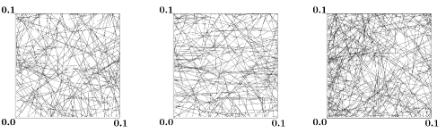
Figure 6.1: The lower left corners ($[0.0,0.1]^{2}$) of the three types of fiber networks analyzed. The left network was generated completely uniformly, the center introduce a bias in fiber rotation, and the right a bias in fiber placement.

All three networks are generated by placing fibers with a fixed length ($r=0.05$) in the unit square until a specified density is achieved. Density in this example is defined as the total edge length, $|1|_{M}^{2}=1000$. Each fiber is placed randomly with its midpoint in $[-0.5r,1+0.5r]^{2}$, then rotated given a random degree. Any part outside the unit square is removed. The slightly extended domain is for uniformity along the boundaries, and in this example, networks are generated with different distributions for the midpoint placement and angle of the fibers. Then every two intersecting fibers are connected by placing a node in each intersection. After this step, any two nodes closer than $r\times 10^{-4}$ are merged, setting a lower bound on the edge lengths. The final step is to remove any potential disconnected edges that have formed along the boundary. Networks generated with these parameters have around 0.3 million network nodes.

To illustrate the homogeneity assumption, $(2R)^{-d}|1|^{2}_{M,B_{R}(x)}$ is presented for the networks discussed. For these networks, five different regular grids are considered; $R^{-1}=4,\ 8,\ 16,\ 32,$ and $64$. For each element in the grids and network types, the corresponding expression $(2R)^{-d}|1|^{2}_{M,B_{R}(x)}$ is evaluated. The evaluations for the uniformly distributed network and the network with biased midpoint placement are illustrated in Figure 6.2, with the numerical results for all the setups presented in Table 6.1

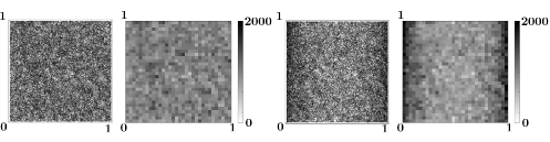
Figure 6.2: Entire networks and illustrations of the homogeneity assumption for the uniform fiber network (left) and the network with more fibers along the lines $x_{1}=0$ and $x_{1}=1$ (right). The boxes represent $(2R)^{-d}|1|^{2}_{M,B_{R}(x)}$ for the respective box $B_{R}(x)$.

The connectivity assumption in Assumption 3.4 is analyzed using subgraphs. The assumption holds if we can find a connected subgraph, $\overline{\mathcal{G}}$, on $B_{R+R_{0}}(x)$. This subgraph has to contain all nodes and edges containing nodes in $B_{R}(x)$, where the second-smallest eigenvalue of the corresponding eigenvalue problem, $\overline{L}u=\lambda_{2}\overline{M}u,$ has the property: $\lambda_{2}^{-1}\leq\mu^{2}R^{2}$, given some constant $\mu>0$ (as discussed in the proof of Lemma 3.5). For simplicity, we only find one such network for each inequality considered, where the network found has a minimal amount of edges using a breadth-first search scheme.

Similar to the homogeneity example, the unit square is partitioned into a regular grid of squares. The inequality induced by each square, $B_{R}(x)$, with length scale $R_{0}^{-1}=64$ for each network is evaluated. In Figure 6.3, the $\lambda_{2}^{-1}\leq\mu^{2}R^{2}$ inequality (connected to the Poincaré inequality) is illustrated. The upper bounds on $\mu$ observed from each grid considered in the connectivity experiments are presented in Table 6.1.

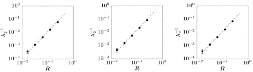
Figure 6.3: The relation between $\lambda_{2}^{-1}$ and $R$ for the following networks: uniform (left), fiber orientation bias (center), and fiber placement bias (right). The dots represent the average $\lambda_{2}^{-1}$ for the given grid size, and the feet the standard deviation.

Table 6.1: Table with $(\sigma,\mu)$ for different $R$ attained through numerical evaluation.

	$R^{-1}=4$	$R^{-1}=8$	$R^{-1}=16$	$R^{-1}=32$	$R^{-1}=64$
Uniform	(1.04,0.49)	(1.08,0.53)	(1.27,0.57)	(1.85,0.675)	(3.42,1.53)
Rand. Orient.	(1.04,0.59)	(1.08,0.61)	(1.27,0.69)	(1.87,0.83)	(2.93,1.35)
Rand. Domain	(1.04,0.53)	(1.57,0.54)	(2.13,0.58)	(3.1,0.76)	(6.86,1.45)

The results illustrate that $\lambda_{2}^{-1}\sim R^{-2}$ for all considered discretization levels, meaning that the considered networks fit the connectivity assumptions down to $R^{-1}=64$. For the worst case scenario considered in Table 6.1 we detect an increase in $\sigma$ and $\mu$ with decreasing $R$ as expected. It is most evident in the finest grid size. It is observable that the network with bias in the fibers’ orientation has lower connectivity than the uniformly distributed network but has similar homogeneity. The network with bias in the fiber midpoint placement has lower homogeneity but comparable connectivity to the non-biased network. Similar results also hold for the corresponding eigenvalue $\lambda_{1}$ related to the Friedrich inequality.

6.2 Heat conductivity

We consider a heat conductivity problem for three different two-dimensional networks ($d=2$). The solutions can be interpreted as the (scalar) temperature in each node, with the operator $K$ defined in equation (3.3). We seek $u\in V=\{v\in\hat{V}\,:\,v(x)=0,x\in\partial\Omega\}$ such that for all $v\in V$,

$$(Ku,v)=(M1,v).$$ (6.1)

We let $f=M1$ in order to distribute the source equally over the edges of the network. An illustration of a solution to such a problem is presented in Figure 6.4.

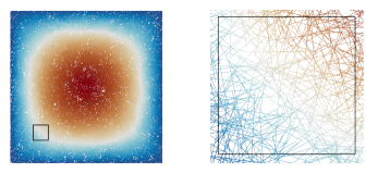
Figure 6.4: Illustrations of the solution to a weighted graph Laplacian problems on the form (6.1). The left picture shows the entire solution, and the right shows the highlighted area in detail.

The networks considered are a uniform regular grid with $(2^{9}+1)^{2}$ nodes, a uniform fiber based network as introduced in Section 6.1 with constant weight $\gamma_{xy}=1$, and a uniform fiber based network with weights $\gamma_{xy}$ drawn from a uniform distribution on $[0.1,1]$. The errors, in $K$-norm, for each iteration with the PCG method is presented in Figure 6.5. The convergence rates, $\tau_{(\ell)}$:

$$\tau_{(\ell)}\vcentcolon=\frac{|\mathbf{u}-\mathbf{u}^{(\ell-1)}|_{\mathbf{K}}}{|\mathbf{u}-\mathbf{u}^{(\ell)}|_{\mathbf{K}}}\leq\tau,\ l=2,\ \ldots$$ (6.2)

on average, $\overline{\tau}$, and upper bounds, $\tau$, for the three cases can be found in Table 6.2. In the figures and results it is clear that the method converges exponentially for all three cases, which is consistent with Theorem 4.3.

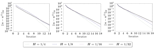
Figure 6.5: The error for each iteration of the three weighted graph Laplacians analyzed. From left to right: constant weights and a uniform regular grid as the network, a fiber based network with constant weights, and a fiber based network with random weights.

Table 6.2: The PCG method’s average and worst convergence rates, $(\overline{\tau},\tau)$, for different heat conductivity problems.

Problem	$H^{-1}=4$	$H^{-1}=8$	$H^{-1}=16$	$H^{-1}=32$
Grid	(0.18,0.31)	(0.25,0.33)	(0.27,0.32)	(0.28,0.31)
Fiber	(0.29,0.48)	(0.33,0.43)	(0.39,0.49)	(0.42,0.47)
Fiber weighted	(0.34,0.44)	(0.40,0.52)	(0.45,0.51)	(0.47,0.54)

6.2.1 Analysis of the constant $C_{d}$

In the following discussion, the theoretical bound on the convergence rate defined by Theorem 4.3 is evaluated closer. Given the theorem and (6.2) we have the following bound:

$$\tau=\frac{\sqrt{\kappa}-1}{\sqrt{\kappa}+1},\ \sqrt{\kappa}=C_{d}\alpha^{-1}\beta\sqrt{\sigma}\mu.$$ (6.3)

With the same approach to the discussion in Section 6.1, values of $\sigma$ and $\mu$ for the uniform regular grid network are numerically evaluated. Together with the convergence results (average) in Table 6.2, and the fact that $\alpha=\beta=1$ for this example, the constant $C_{d}$ in Theorem 4.3 can be approximated by

$$C_{d}=\frac{1+\overline{\tau}}{\sqrt{\sigma}\mu(1-\overline{\tau})}.$$

The geometric constants and the approximations of $C_{d}$ are presented in Table 6.3. From these results, it is clear that the constant $C_{d}\approx 3.5$ bounds the average convergence rates for all the grids analyzed for the regular grid network.

Table 6.3: Investigation of the constant $C_{d}$ using the average convergence rates, $\overline{\tau}$, and the geometrical constants $\sigma$ and $\mu$ for the regular grid network.

	$H^{-1}=4$	$H^{-1}=8$	$H^{-1}=16$	$H^{-1}=32$
$\sigma$	1.0	1.0	1.1	1.1
$\mu$	0.45	0.47	0.48	0.51
$C_{d}$	3.2	3.5	3.5	3.2

The convergence results for the grid type network is now compared to the convergence results for the uniformly distributed fiber based network without weights. In Section 6.1, the geometrical constants $\sigma$ and $\mu$ were evaluated for the fiber based network. Using (6.3) with the constants in Table 6.1, $C_{d}=3.5$, and the convergence rates in Table 6.2, the convergence rate of the PCG method on the fiber model is compared to

$$\tilde{\tau}=\frac{\sqrt{\kappa}-1}{\sqrt{\kappa}+1},\ \sqrt{\kappa}=3.5\sqrt{\sigma}\mu$$

in Table 6.4.

Table 6.4: Comparing convergence rate estimates, $\tilde{\tau}$, with average convergence rates, $\overline{\tau}$, in numerical experiments for a fiber based network.

	$H^{-1}=4$	$H^{-1}=8$	$H^{-1}=16$	$H^{-1}=32$
$\overline{\tau}$	0.29	0.33	0.39	0.42
$\tilde{\tau}$	0.27	0.35	0.45	0.60

The convergence estimates in Table 6.4 are similar to the numerical results except for the last data point. In that case, the convergence rate of the PCG method converges faster than the estimate. With this in mind, it is clear that the convergence rates are affected by the homogeneity and connectivity constants $\sigma$ and $\mu$. Moreover, a similar geometric constant bounds the average convergence rates of the PCG method for the girds analyzed. We conclude that the error is reduced by a constant factor in each iteration, in agreement with Theorem 4.3. In addition, the bound appears to be sharp in the dependency of $\sigma^{1/2}$ and $\mu$ with a proportionality constant $C_{d}\approx 3.5$ on coarser scales $H$.

6.3 Structural problem for fiber based material

Here two variations of Example 3.3 is presented, where the networks should be interpreted as an anisotropic mesh of round steel wires with radius $r_{w}=2.5\times 10^{-3}$ m. Equation (3.4) becomes a linearized version of Hooke’s law with parameter $\gamma_{xy}=\gamma_{1}=AE$, where $A=\pi r_{w}^{2}$ is the cross-section area of the wire and $E=210$ GPa the wires Young’s modulus. The bending forces are handled by the addition of the equations in (3.5). These additions are linearized versions of Euler–Bernoulli beam theory with parameters $\gamma_{xyz}=EI(|x-y|+|x-z|)^{-2}$ where $E$ is the same Young’s modulus and $I=0.25\pi r_{w}^{4}=0.25Ar_{w}^{2}$ is the second moment of area of the wire. The two coefficients have the following relation,

$$\gamma_{xyz}=EA\frac{r_{w}^{2}}{4(|x-y|+|x-z|)^{2}}=\gamma_{1}\frac{r_{w}^{2}}{4(|x-y|+|x-z|)^{2}},$$

where $0.05\leq\frac{r_{w}}{|x-y|}\leq 500$ for any edge $x\sim y$.

6.3.1 Pure displacement problem

The first structural problem is a tensile simulation, where one side is fixed, and the other is displaced, straining the network. For this experiment, the second fiber-based network in Section 6.1 is used. This network places the fibers uniformly in the domain but with rotational bias. We only consider forces and displacements in the plane the network resides in for this simulation, meaning that the lateral component is left out. We apply non-homogeneous Dirichlet boundary conditions on the two fixed sides of $\Omega$ and seek $\hat{\mathbf{u}}=\mathbf{u}+\mathbf{g}$ where $\mathbf{u}\in\mathbf{V}$ and $\mathbf{g}(x)=[0.2x_{1},0]$. We define $\Gamma=\{x=(x_{1},x_{2})\in\partial\Omega\,:\,x_{1}=0\text{ or }x_{1}=1\}$ and solve for $\mathbf{u}\in\mathbf{V}=\{\mathbf{v}\in\hat{\mathbf{V}}\,:\,\mathbf{v}(x)=0,x\in\Gamma\}$ such that for all $v\in V$,

$$(\mathbf{K}\mathbf{u},\mathbf{v})=-(\mathbf{K}\mathbf{g},\mathbf{v}).$$

The problem is solved using a direct solver and the PCG method. An illustration of the solution and the errors in each iteration of the PCG method are presented in Figure 6.6, with average convergence rates presented in Table 6.5. The PCG method converges exponentially, and with $\alpha=0.05$ and $\beta=500$ the method converges substantially faster than the theoretical upper bound.

Figure 6.6: The displaced network along with the convergence results for the PCG method on the two-dimensional structural problem.

Table 6.5: Average convergence rates, $\overline{\tau}$, for the two-dimensional structural problem.

	$H^{-1}=4$	$H^{-1}=8$	$H^{-1}=16$	$H^{-1}=32$
$\overline{\tau}$	0.54	0.62	0.65	0.65

6.3.2 Displacement problem with lateral load

Table 6.6: Average convergence rates, $\overline{\tau}$, for the three-dimensional structural problem.

	$H^{-1}=4$	$H^{-1}=8$	$H^{-1}=16$	$H^{-1}=32$
$\overline{\tau}$	0.56	0.64	0.74	0.76

In the second numerical example of the structural problem, we introduce a lateral load to the previous tensile problem with half the strain. This results in a model with $d=2$ and $n=3$. Using the same $\Gamma$ as in the previous numerical example and $\mathbf{V}$ defined analogously, the problem is to find $\mathbf{u}\in\mathbf{V}$ such that for all $\mathbf{v}\in\mathbf{V}$,

$$(\mathbf{K}\mathbf{u},\mathbf{v})=(\mathbf{M}\mathbf{g}^{\prime}-\mathbf{K}\mathbf{g},\mathbf{v})\\$$

where $\mathbf{g}^{\prime}=[0,0,-10^{3}]$ and $\mathbf{g}(x)=[0.1x_{1},0,0]$. The network is the third fiber based network in Section 6.1. In this network, the fibers are placed with a bias in the domain, resulting in higher densities along the $x_{2}$-axis. The solution and convergence results for the domain decomposition method for this setup is presented in Figure 6.7 and Table 6.6. Similar to the two-dimensional case, the convergence is exponential, and the rates observed are better than the theoretical bound.

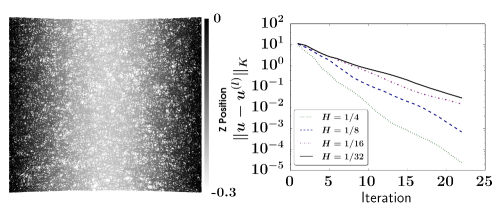
Figure 6.7: The solution to the exact problem $\mathbf{u}$, along with the convergence results for the PCG method for different $H$.

Acknowledgements.

The first author is supported by the Swedish Foundation for Strategic Research (SSF). The second and third author are supported by the Göran Gustafsson Foundation for Research in Natural Sciences and Medicine and the Swedish Research Council (project number 2019-03517).

Appendix

For completeness we include the proof of Lemma 4.2

Proof.

First we prove the relation

$$C_{1}^{-1}|\mathbf{v}|_{\mathbf{K}}^{2}\leq(\mathbf{K}\mathbf{P}\mathbf{v},\mathbf{v})\leq C_{2}|\mathbf{v}|_{\mathbf{K}}^{2}$$ (6.4)

for all $\mathbf{v}\in\mathbf{V}$.

The Cauchy-Schwarz inequality gives

$$|\mathbf{v}|_{\mathbf{K}}^{2}=\sum_{j=0}^{m}(\mathbf{K}\mathbf{v},\mathbf{v}_{j})=\sum_{j=0}^{m}(\mathbf{K}\mathbf{P}_{j}\mathbf{v},\mathbf{v}_{j})\leq\left(\sum_{j=0}^{m}|\mathbf{P}_{j}\mathbf{v}|^{2}_{\mathbf{K}}\right)^{1/2}\left(\sum_{j=0}^{m}|\mathbf{v}_{j}|_{\mathbf{K}}^{2}\right)^{1/2}.$$

Since $\mathbf{P}_{j}$ is $\mathbf{K}$-orthogonal $\sum_{i=0}^{m}|\mathbf{P}_{j}\mathbf{v}|_{\mathbf{K}}^{2}=\sum_{j=0}^{m}(\mathbf{K}\mathbf{P}_{j}\mathbf{v},\mathbf{v})=(\mathbf{K}\mathbf{P}\mathbf{v},\mathbf{v})$ and by Lemma 4.1 $\sum_{i=0}^{m}|\mathbf{v}_{j}|_{\mathbf{K}}^{2}\leq C_{1}|\mathbf{v}|_{\mathbf{K}}^{2}$. We conclude $|\mathbf{v}|_{\mathbf{K}}^{2}\leq C_{1}(\mathbf{K}\mathbf{P}\mathbf{v},\mathbf{v}).$ For the second inequality we again use Lemma 4.1 and get

$$(\mathbf{K}\mathbf{P}\mathbf{v},\mathbf{v})\leq\left|\sum_{j=0}^{m}\mathbf{P}_{j}\mathbf{v}\right|_{\mathbf{K}}|\mathbf{v}|_{\mathbf{K}}\leq\left(C_{2}\sum_{j=0}^{m}|\mathbf{P}_{j}\mathbf{v}|^{2}_{\mathbf{K}}\right)^{1/2}|\mathbf{v}|_{\mathbf{K}}\leq\left(C_{2}(\mathbf{K}\mathbf{P}\mathbf{v},\mathbf{v})\right)^{1/2}|\mathbf{v}|_{\mathbf{K}}.$$

Equation (6.4) follows by division by $(\mathbf{K}\mathbf{P}\mathbf{v},\mathbf{v})^{1/2}$ and squaring the equation.

The spectral theorem for finite dimensional real spaces guarantees the existence of eigenfunctions $\{\mathbf{z}_{i}\}_{i=1}^{l}$ to the $\mathbf{K}$-symmetric operator $\mathbf{P}$:

$$(\mathbf{K}\mathbf{P}\mathbf{z}_{i},\mathbf{v})=\lambda_{i}(\mathbf{K}\mathbf{z}_{i},\mathbf{v})$$

for all $\mathbf{v}\in\mathbf{V}$. The eigenfunctions form an orthonormal basis of $\mathbf{V}$ i.e. $(\mathbf{K}\mathbf{z}_{i},\mathbf{z}_{j})=\delta_{ij}$. Furthermore, using equation (6.4) we get

$$C_{1}^{-1}|\mathbf{z}_{i}|_{\mathbf{K}}^{2}\leq(\mathbf{K}\mathbf{P}\mathbf{z}_{i},\mathbf{z}_{i})\leq C_{2}|\mathbf{z}_{i}|^{2}_{\mathbf{K}},$$

and conclude

$$C_{1}^{-1}\leq\lambda_{i}\leq C_{2},$$ (6.5)

for all $i=1,\dots,l$ which proves the first statement of the lemma. With the eigenfunction expansion $\mathbf{v}=\sum_{i=1}^{l}\alpha_{i}\mathbf{z}_{i}$ the second part follows directly by

$$\frac{|p(\mathbf{P})\mathbf{v}|^{2}_{\mathbf{K}}}{|\mathbf{v}|_{\mathbf{K}}^{2}}=\frac{\sum_{i,j=1}^{l}\alpha_{i}\alpha_{j}(\mathbf{K}p(\mathbf{P})\mathbf{z}_{i},p(\mathbf{P})\mathbf{z}_{j})}{\sum_{i=1}^{l}\alpha_{i}^{2}}$$

$$=\frac{\sum_{i=1}^{l}\alpha_{i}^{2}p(\lambda_{i})^{2}}{\sum_{i=1}^{l}\alpha_{i}^{2}}\leq\max_{1\leq i\leq l}|p(\lambda_{i})|\leq\max_{\lambda\in[C_{1}^{-1},C_{2}]}|p(\lambda)|.$$

∎

References

- [1] Blunt. M. J., Bijeljic, B., Dong, H., Gharbi, O., Iglauer, S., Mostaghimi, P., Paluszny, A., and Pentland, C., Pore-scale imaging and modelling, Advances in water resources, 51 (2013), pp. 197–216.
- [2] Brandt, A., Multi-level adaptive solutions to boundary-value problems, Mathematics of Computation, 31 (1977) pp. 333–390.
- [3] Cheeger J., A lower bound for the smallest eigenvalue of the Laplacian, Problems in Analysis, R. C. Gunning (Editor), Princeton U.P., 1970, pp. 195–199.
- [4] Chung, F., Discrete Isoperimetric Inequalities, Surveys in Differential Geometry IX, International Press, (2004), pp. 53–82.
- [5] Chung, F., Spectral Graph Theory, American Mathematical Society, Providence, 1997.
- [6] Chung, F., Grigor’yan, A., and Yau, S.-T., Higher eigenvalues and isoperimetric inequalities on Riemannian manifolds and graphs, Communications on Analysis and Geometry, 8 (2000), pp. 969–1026.
- [7] Chung, F. and Yau, S.-T., Eigenvalues of graphs and Sobolev inequalities, Combinatorics, Probability and Computing, 4 (1995), pp. 11–26.
- [8] Clément, P. Approximation by finite element functions using local regularization, Rev. Française Automat. Informat. Recherche Opérationnelle Sér. Rouge Anal. Numér., 9, R-2 (1975), pp. 77–84.
- [9] Fiedler, M., Algebraic connectivity of graphs, Czechoslovak Mathematical Journal, 23(2) (1973), pp. 298–305.
- [10] Friedland, S., Lower bounds for the first eigenvalue of certain M-matrices associated with graphs, Linear Algebra Appl., 172 (1992), pp. 71–84.
- [11] Gergelits, T. and Strakoš, Z. Composite convergence bounds based on Chebyshev polynomials and finite precision conjugate gradient computations, Numerical algorithms, 4 (2014).
- [12] Gjennestad, M., Vassvik, M., Kjelstrup, S., and Hansen, A., Stable and efficient time integration of a pore network model for two-phase flow in porous media, Front. Phys., 6 (2018).
- [13] Heyden, S., Network modelling for the evolution of mechanical properties of cellulose fibre fluff, Doctoral thesis, Department of mechanics and materials, Lund University, 2000.
- [14] Huang, X., Zhou, W., and Deng, D. Validation of pore network modeling for determination of two-phase transport in fibrous porous media, Sci Rep, 10, 20852 (2020).
- [15] Iliev, O., Lazarov, R., and Willems, J., Fast numerical upscaling of heat equation for fibrous materials, Comput. Visual. Sci., 13 (2010), pp. 275–285.
- [16] Kettil, G., Målqvist, A., Mark, A., Fredlund, M., Wester, K., and Edelvik, F., Numerical upscaling of discrete network models, BIT 60 (2020), pp. 67–92.
- [17] Kornhuber R., Peterseim D., and Yserentant, H., An analysis of a class of variational multiscale methods based on subspace decomposition, Mathematics of Computation, 87(314):2765-2774, 2018.
- [18] Kornhuber, R. and Yserentant, H., Numerical homogenization of elliptic multiscale problems by subspace decomposition, Multiscale Model. Simul. 14(3) (2016), 1017–1036.
- [19] Målqvist, A. and Peterseim, D., Computation of eigenvalues by numerical upscaling, Numer. Math. 130 (2015), 337–361.
- [20] Målqvist, A. and Peterseim, D., Numerical homogenization by localized orthogonal decomposition, SIAM Spotlights, ISBN: 978-1-611976-44-1, 2020.
- [21] Saad, Y., Iterative methods for sparse linear systems, 2nd edition, SIAM, 2003.
- [22] Tillich, J.-P., Edge isoperimetric inequalities for product graphs, Discrete Mathematics, 213 (2000), pp. 291–320.
- [23] Smith, B., Bjørstad, P., and Gropp, W., Domain Decomposition, Parallel Multilevel Methods for Elliptic Partial Differential Equations, Cambridge University Press, 1996.
- [24] Stüben, K., A review of algebraic multigrid, J. Comp. Appl. Math., 128, (2001), pp. 281–309.
- [25] Xu J., Iterative Methods by Space Decomposition and Subspace Correction, SIAM Review, 34, (1992), pp. 581–613.
- [26] Xu, J. and Zikatanov, L., Algebraic multigrid methods, Acta Numerica, 26, (2017), pp. 591–721.